Phase transitions in a non-Hermitian Su-Schrieffer-Heeger model via Krylov spread complexity

Abstract

We investigate phase transitions in a non-Hermitian Su–Schrieffer–Heeger (SSH) with an imaginary chemical potential via Krylov spread complexity and Krylov fidelity. The spread witnesses the $\mathcal{PT}$-transition for the non-Hermitian Bogoliubov vacuum of the SSH Hamiltonian, where the spectrum goes from purely real to complex (oscillatory dynamics to damped oscillations). In addition, it also witnesses the transition occurring in the $\mathcal{PT}$-broken phase, where the spectrum goes from complex to purely imaginary (damped oscillations to sheer decay). For a purely imaginary spectrum, the Krylov spread fidelity, which measures how the time-dependent spread reaches its stationary state value, serves as a probe of previously undetected dynamical phase transitions.

I Introduction

Krylov complexity plays an essential role in understanding quantum dynamics, as it measures the spread of an operator (or state) in a natural basis spanning the underlying subspace where the time evolution takes place. This complexity measure was initially used in the context of operators evolving under chaotic many-body Hamiltonians, where it was hypothesized that the Lacnzos coefficients of chaotic quantum systems should grow as fast as possible and be asymptotically linear in the basis numbering, implying, thus, an exponential growth in time of the Krylov complexity Parker et al. (2019). These coefficients are obtained when the evolution-produced orthonormal basis is constructed from the repeated action of the generator of the dynamics and the initial state or operator, and their statistics have not only proven to be useful in probing chaotic dynamics alone but also to detect integrability, localization, and the transition from such phases to chaotic ones Zhou et al. (2025); Hashimoto et al. (2023); Balasubramanian et al. (2020); Rabinovici et al. (2022a, 2021, b); Trigueros and Lin (2022); Bhattacharya et al. (2024a); Balasubramanian et al. (2023); Sahu et al. (2023). Krylov complexity has also been used to detect those transitions and phases by studying, e.g., how and when it reaches its saturation value Español and Wisniacki (2023); Alishahiha et al. (2024); Erdmenger et al. (2023); Scialchi et al. (2024); Ganguli (2024).

Other more standard complexity measures such as, e.g., circuit complexity Chi-Chih Yao (1993); Haferkamp et al. (2022) and Nielsen complexity Nielsen et al. (2006); Dowling and Nielsen (2006); Nielsen (2006) can be seen as less “canonical” as they require the introduction of penalty factors, universal gates, and tolerance bounds, among other properties. Relations between Krylov complexity and other complexity measures are expected as the latter is, in a way, a more natural measure. Indeed, it has been shown that Krylov complexity can be seen as an upper bound of circuit Lv et al. (2024) and Nielsen Craps et al. (2024) complexities, indicating, thus, that Krylov complexity is a bona fide measure of complexity.

Applications of Krylov complexity beyond its initial scope have been found. For example, it has been used as a probe to distinguish topological phases in spin chains  Caputa et al. (2023); Caputa and Liu (2022), dynamical phase transitions emerging from quantum quenches Bento et al. (2024), Trotter transitions Suchsland et al. (2025), Zeno effect Bhattacharya et al. (2024b), among many other applications Xia et al. (2024); Beetar et al. (2024); Guerra et al. (2025); Hörnedal et al. (2022); Carabba et al. (2022); Gill and Sarkar (2024); Bhattacharya et al. (2024c); Gautam et al. (2024); Patramanis and Sybesma (2024); Zhou and Yu (2022). We remark that Krylov complexity has been heavily studied in the context of open systems governed by Lindbladian dynamics (see, e.g., Refs. Liu et al. (2023); Carolan et al. (2024); Bhattacharjee et al. (2023); Bhattacharya et al. (2022, 2023)). For a recent review on Krylov complexity in general, see Ref. Nandy et al. (2024a). The term Krylov complexity is used in the Heisenberg picture, whereas Krylov spread complexity or spread complexity is used in the Schrödinger picture. In this work, we focus on Krylov spread and use the three terms interchangeably.

Despite the aforementioned applications of Krylov complexity, its relation with measurement-induced entanglement phase transitions Gal et al. (2023); Turkeshi and Schiró (2023); Turkeshi et al. (2021); Poboiko et al. (2025) has not been fully understood: while the entanglement entropy is calculated in subregions of the system, Krylov complexity is calculated for the entire system (see, e.g., Ref. Alishahiha and Banerjee (2023) for a discussion on this matter). For example, it is known that in a monitored 1D Ising chain with a transverse magnetic field in the zero-click limit, there is an entanglement entropy transition from logarithmic law when the imaginary part of the spectrum is gapless to an area law when it is gapped Zerba and Silva (2023). For the same model, in Ref. Guerra et al. (2025), it was shown that the second derivatives of the Krylov density with respect to the magnetic field and measurement rate display an algebraic divergent behavior when the imaginary part of the spectrum goes from gapless to gapped. Therefore, this seems to indicate that the derivatives of the Krylov complexity display either discontinuities or divergences when the spectrum undergoes certain changes, e.g., when it goes from gapful to gapless, when it displays non-analyticities, etc. This conjecture, if true, could be used to analyze other quantum phase transitions that are either difficult to calculate with more standard measures or that have not been discovered.

In this spirit, systems possessing parity and time-reversal ($\mathcal{PT}$-) symmetry Bender and Hook (2024); Bender (2015); Meden et al. (2023) are ideal for testing the above conjecture further, as their associated spectrum is real in the $\mathcal{PT}$-symmetric phase and can become complex, as well as purely imaginary, in the $\mathcal{PT}$-broken phase. To address this issue, we consider a $\mathcal{PT}$-symmetric non-Hermitian Su-Schrieffer-Heeger (SSH) model with a complex chemical potential. It was shown in Ref. Gal et al. (2023) that the entanglement entropy of this model obeys a volume law in the parameter space correspondent to the $\mathcal{PT}$-symmetric phase as well as in a subregion where this phase is broken. Within the $\mathcal{PT}$-broken phase, a volume-to-area transition in the entanglement entropy was found when the spectrum goes from complex to purely imaginary. Remarkably, as we demonstrate in this work, the derivatives of the Krylov spread complexity calculated in the non-Hermitian Bogoliubov vacuum of the non-Hermitian SSH Hamiltonian distinguishes the two types of phase transitions by displaying a non-analytic behavior across the parameter space. In addition, by implementing the Krylov fidelity introduced in Ref. Guerra et al. (2025), which describes how the complexity reaches its stationary state, we are able to refine part of the $\mathcal{PT}$-broken phase corresponding to a purely imaginary and gapped spectrum and find two additional dynamical phases. We point out that Krylov complexity has been studied in systems having $\mathcal{PT}$ symmetry Beetar et al. (2024); Bhattacharya et al. (2024b), where it was found that it distinguishes between the $\mathcal{PT}$-symmetric and broken phases. However, this was done mainly by studying the behavior of complexity over time, and previously unseen dynamical phases were not reported.

This work is organized as follows. In Sec. II, we define the non-Hermitian SSH Hamiltonian and describe its spectrum. In Sec. III, we briefly, introduce the Krylov spread complexity of states. In Sec. IV, we discuss the Krylov spread complexity of a Hermitian evolution taking a particular initial state to the non-Hermitian vacuum of the SSH Hamiltonian. We demonstrate that the second derivative of the spread with respect to one of the parameters either diverges or is discontinuous at the boundaries between regions where the spectral properties of the Hamiltonian change. Namely, when it goes from real to complex or purely imaginary and vice versa. In Sec. V, we find the Krylov spread of the evolution of the same initial state used in the unitary evolution, but this time via the non-Hermitian SSH Hamiltonian when its spectrum is purely imaginary. We define the stationary state time and find two dynamical phase transitions dictated by it. Finally, we present the conclusions and summary in Sec. VI.

II Model

Consider the SSH model obeying anti-periodic boundary conditions with $L$ sites and with an imaginary chemical potential Gal et al. (2023); Lieu (2018a)

$$H=\sum_{n=1}^{L}\left(t_{1}c^{\dagger}_{A,n}d_{B,n}+t_{2}c^{\dagger}_{A,n}d_{B,n-1}+\text{H.c.}\right)\\ +i\gamma\sum_{n=1}^{L}\left(c_{A,n}^{\dagger}c_{A,n}+d^{\dagger}_{B,n}d_{B,n}\right),$$ (1)

where $\gamma\in\mathbb{R}$, and $c_{A,n}$ and $d_{B,n}$ are the fermionic operators of the sublattices $A$ and $B$, respectively. For convenience, we set the intracell and intercell hoppings as $t_{1}=-J-h/2$ and $t_{2}=-J+h/2$, respectively, where $h\in\mathbb{R}$, and $J>0$ is fixed. The anti-Hermitian part of the Hamiltonian can be thought of as the result of the backaction of a continuous measurement of the local density of particles and holes on the sublattices $A$ and $B$, respectively, where no click was detected Breuer and Petruccione (2007).

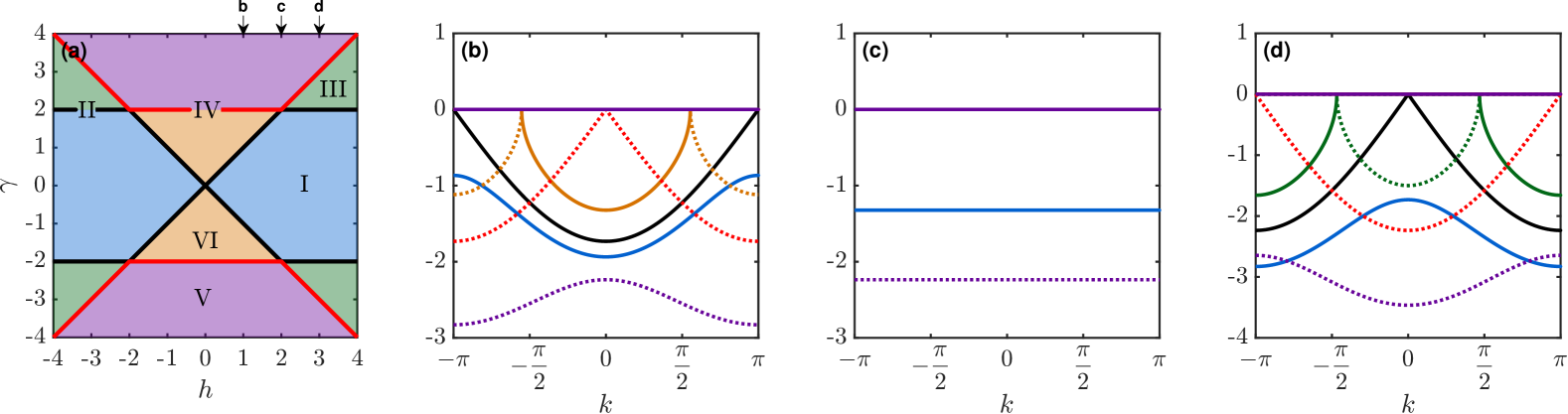
Figure 1: Negative part of the spectrum (6) in terms of the parameters $(J=1,h,\gamma).$ Panel (a) displays the $h$-$\gamma$ plane with the six subsets I-VI indicated in the main text. Panels (b)-(d) display the real (solid lines) and imaginary (dotted lines) parts of $-\Lambda(k)$ for several values of $(h,\gamma)$. Specifically, in Panel (b), $h=1$ and $\gamma\in\{1/2,1,3/2,2,3\}$; in panel (c), $h=2$ and $\gamma\in\{3/2,2,3\}$; in panel (d), $h=3$ and $\gamma\in\{1,2,5/2,3,4\}$. These values of $(h,\gamma)$ go from the bottom to the top in the diagram (a), each lying in only one of the regions. Thus, the colors in (b)-(d) correspond to the position of the ordered pair $(h,\gamma)$ in the diagram (a).

The Hamiltonian (1) can be diagonalized by implementing the Fourier representation (see Appendix A)

$$\begin{pmatrix}c_{A,n}\\ d_{B,n}\end{pmatrix}=\dfrac{e^{-i\frac{\pi}{4}\sigma_{x}}}{\sqrt{L}}\sum_{k\in\mathcal{K}}e^{ikn}\begin{pmatrix}c_{k}\\ d_{k}\end{pmatrix},$$ (2)

where $\sigma_{x}$ is a Pauli matrix, and

$$\mathcal{K}=\left\{k_{n}=\dfrac{2\pi}{L}\left(-\Bigg{\lceil}\frac{L-1}{2}\Bigg{\rceil}+n+\frac{1}{2}\right):n\in[0,L)\cap\mathbb{N}\right\}$$ (3)

is the momenta set in the first Brillouin zone, giving

$$H=\sum_{k}\Lambda(k)\left(\chi_{+,k}^{*}\chi_{+,k}-\chi_{-,k}^{*}\chi_{-,k}\right).$$ (4)

Here, $\chi_{\pm,k}$ are non-Hermitian quasiparticle fermionic operators obeying the anti-commutation relations

$$\{\chi_{s,k}^{*},\chi_{s^{\prime},k^{\prime}}\} =\delta_{ss^{\prime}}\delta_{kk^{\prime}},\quad\{\chi_{s,k}^{*},\chi_{s^{\prime},k^{\prime}}^{*}\}=0,$$

$$\{\chi_{s,k},\chi_{s^{\prime},k^{\prime}}\} =0.$$ (5)

The non-hermiticity also implies $\chi_{s,k}^{\dagger}\neq\chi_{s,k}^{*}$. The relations between the non-Hermitian operators and the sublattice operators $c$ and $d$ are given in Eqs. (37) and (38). The spectrum of $H$ is

$$\pm\Lambda(k) =\pm\sqrt{h^{2}-\gamma^{2}+(4J^{2}-h^{2})\cos^{2}\dfrac{k}{2}}$$ (6a)

$$\equiv\pm E(k)\pm i\Gamma(k),$$ (6b)

where $E(k)\coloneqq\mathfrak{Re}\,\Lambda(k)$ and $\Gamma(k)\coloneqq\mathfrak{Im}\,\Lambda(k).$ For a given $k\in\mathcal{K}$, $\Lambda(k)$ is either real or imaginary, and it completely vanishes at the points

$$\pm k_{\text{EP}}=\pm 2\arccos\sqrt{\dfrac{\gamma^{2}-h^{2}}{4J^{2}-h^{2}}},$$ (7)

which correspond to two exceptional points (EPs) Heiss (2012). Based on the above features, we identify the following six subregions in the $h$-$\gamma$-plane displayed in Fig. 1(a):

1. $\{\absolutevalue{\gamma}<\absolutevalue{h},\absolutevalue{h}\leq 2J\}\cup\{\absolutevalue{\gamma}<2J,\absolutevalue{h}\geq 2J\}$. $E(k)$ is gapped, i.e., $E(k)\neq 0$, and $\Gamma(k)\equiv 0$.

2. $\{\absolutevalue{\gamma}=\absolutevalue{h},\absolutevalue{h}\leq 2J\}\cup\{\absolutevalue{\gamma}=2J,\absolutevalue{h}\geq 2J\}$. $\Gamma(k)\equiv 0$ and $E(k)$ is gapless at $\pm k_{\text{EP}}=\pm\pi$ for $h<2J$, and at $k_{\text{EP}}=0$ for $h>2J$. $\Lambda(k)\equiv 0$ for $h=\gamma=2J.$

3. $\{2J<\absolutevalue{\gamma}<\absolutevalue{h},\absolutevalue{h}>2J\}$. $E(k)=0$ for $\absolutevalue{k}\leq k_{\text{EP}}$ and $\Gamma(k)=0$ for $\absolutevalue{k}\geq k_{\text{EP}}$.

4. $\{\absolutevalue{\gamma}=2J,\absolutevalue{h}\leq 2J\}\cup\{\absolutevalue{\gamma}=\absolutevalue{h},\absolutevalue{h}\geq 2J\}$. $E(k)\equiv 0$ and $\Gamma(k)$ is gapless at $k_{\text{EP}}=0$ for $h\leq 2J$, and at $\pm k_{\text{EP}}=\pm\pi$.

5. $\{\absolutevalue{\gamma}>2J,\absolutevalue{h}\leq 2J\}\cup\{\absolutevalue{\gamma}>\absolutevalue{h},\absolutevalue{h}\geq 2J\}$. $\Gamma(k)$ is gapped and $E(k)\equiv 0.$

6. $\{\absolutevalue{h}<\absolutevalue{\gamma}<2J,0<\absolutevalue{h}<2J\}$. $\Gamma(k)=0$ for $\absolutevalue{k}\leq k_{\text{EP}}$ and $E(k)=0$ for $\absolutevalue{k}\geq k_{\text{EP}}$.

The reason the spectrum is purely real in regions I and II, even though the Hamiltonian (1) is not Hermitian, is due to $\mathcal{PT}$-symmetry Gal et al. (2023); Rottoli et al. (2024); Bender and Hook (2024); Bender (2015), where $\mathcal{P}$ is the parity operator defined as

$$\mathcal{P}c_{A,n}\mathcal{P}=d_{B,L-n+1},\quad\mathcal{P}d_{B,n}\mathcal{P}=c_{A,L-n+1},$$ (8)

and $\mathcal{T}$ is the anti-unitary time-reversal operator defined as $\mathcal{T}\lambda\mathcal{T}=\lambda^{*}$, for $\lambda\in\mathbb{C}$. Thus, regions I and II correspond to a $\mathcal{PT}$-symmetric phase, and the other regions correspond to a$\mathcal{PT}$-broken phases.

III Spread complexity of states

Here, we briefly review the Krylov spread complexity of states to establish further notation. We shall not address the Krylov complexity of density matrices and operators. For a recent review, see Ref. Nandy et al. (2024a).

Let $H$ be the Hamiltonian generating the dynamics $e^{-iHt}\ket{\psi(0)}$, where $\ket{\psi(0)}\in\mathcal{H}$ is some initial state. The Krylov space generated by the initial state and the Hamiltonian is

$$\mathfrak{K}\big{(}\psi(0),H\big{)}\!=\text{span}\left\{\ket{\psi(0)}\!,H\ket{\psi(0)}\!,\ldots,H^{n}\ket{\psi(0)}\!,\ldots\right\}.$$ (9)

By implementing the Gram-Schmidt orthonormalization procedure to the linearly-independent set of vectors from the ordered set $\{H^{n}\ket{\psi(0)}\}_{n\geq 0}$, one can find the ordered basis, called Krylov basis, $\{\ket{K_{n}}\}_{n}$, where $n=0,\ldots,\text{dim}\,\mathfrak{K}\leq\text{dim}\,\mathcal{H}$ and $\ket{K_{0}}=\ket{\psi(0)}$. Hence, the non-Hermitian and evolution can be expanded in terms of this basis as $\ket{\psi(t)}=\sum_{n=0}^{\text{dim}\,\mathfrak{K}}\varphi_{n}(t)\ket{K_{n}}$, where $\varphi_{n}(t)=\bra{K_{n}}\ket{\psi(t)}$. Thus, the Krylov spread complexity of the evolved state $\ket{\psi(t)}$ is defined as

$$C(\psi(0),H;t)\equiv\mathcal{C}(t)=\sum_{n=0}^{\text{dim}\,\mathfrak{K}}n\absolutevalue{\varphi_{n}(t)}^{2},$$ (10)

and it measures the mean value of the evolved state on the Krylov basis. As it was shown in Ref. Balasubramanian et al. (2022), Eq. (10) is the spread that minimizes $\sum_{n}n\absolutevalue{\bra{\phi(t)}\ket{B_{n}}}^{2}$ over all possible ordered basis $\{\ket{B}_{n}\}_{n}$.

The above construction also holds for non-Hermitian Hamiltonians and is what we implement in this work. Other approaches such as, e.g., the bi-Lanczos algorithm Nandy et al. (2024a); Bhattacharya et al. (2023), and the singular-value decomposition Nandy et al. (2024b), among others, focus on different ways of obtaining the Krylov basis. Those methods are implemented primarily for computational reasons, and we do not use them in our analysis.

IV Krylov spread via unitary dynamics

In what follows, we calculate the Krylov spread density of a state that evolves unitarily to the non-Hermitian vacuum of $H$. We demonstrate that the second derivatives of the spread density with respect to $\gamma$ display a non-analytic behavior in regions II and IV, implying that this complexity measure can detect the $\mathcal{PT}$-symmetry breaking as well as the spectral transition from a complex to a purely imaginary spectrum which is the mechanism responsible for the volume-to-area entanglement phase transition reported in Ref. Gal et al. (2023).

Consider the two Hermitian Hamiltonians

$$H_{0}=-\sum_{k\in\mathcal{K}}\left(J+\frac{h}{2}\right)\sin k\left(c_{k}^{\dagger}c_{k}-d_{k}^{\dagger}d_{k}\right).$$ (11)

and

$$\hat{H}=\sum_{k\in\mathcal{K}^{+}}\left(iy_{+}(k)c_{k}^{\dagger}d_{k}+iy_{-}(k)d^{\dagger}_{-k}c_{-k}-\text{H.c.}\right),$$ (12)

where

$$y_{\pm}(k)=-\dfrac{t_{1}+t_{2}\cos k\mp\gamma}{\sqrt{t_{1}^{2}+t_{2}^{2}-\gamma^{2}+2t_{1}t_{2}\cos k}+t_{2}\sin k}.$$ (13)

Let $\ket{0}$ be the vacuum annihilated by $c_{k}$ and $d_{k}$ for any $\in\mathcal{K}$, and consider the ground state of $H_{0}$,

$$\ket{\psi(0)}=\ket{\text{GS}}=\prod_{k\in\mathcal{K}^{+}}c_{-k}^{\dagger}d_{k}^{\dagger}\ket{0}.$$ (14)

It turns out that if we evolve this state via $\hat{H}$, we reach the ground state of Eq. (1),

$$\ket{\Omega}=\prod_{k\in\mathcal{K}^{+}}\dfrac{\chi_{-,-k}^{*}\chi_{-,k}^{*}}{\bra{0}(\chi_{-,-k}^{*}\chi_{-,k}^{*})^{\dagger}\chi_{-,-k}^{*}\chi_{-,k}^{*}\ket{0}^{1/2}}\ket{0}.$$ (15)

As we show in Appendix A, $\hat{H}$ is induced by the unitary operator $\Omega\in\text{SU}(2)^{\otimes L}/\text{U}(1)^{\otimes L}$, satisfying $\ket{\Omega}=\Omega\ket{\text{GS}}$. In other words, $\ket{\Omega}$ is a generalized coherent state of $\ket{\text{GS}}$, and $\ket{\psi(1)}=e^{-i\hat{H}}\ket{\text{GS}}=\Omega\ket{\text{GS}}$.

Moreover, as $\ket{\text{GS}}$ is the lowest weight $\mathfrak{su}(2)\times\mathfrak{su}(2)$-state, the spread per site (or spread density) of $\ket{\psi(1)}=\ket{\Omega}$ is given by the thermodynamic limit of the sum over complexity spread of each mode Caputa and Liu (2022); Caputa et al. (2023)

$$\mathcal{C}_{\Omega} \coloneqq\lim_{L\to\infty}\dfrac{1}{L}\sum_{\begin{subarray}{c}k\in\mathcal{K}^{+}\\ s=\pm\end{subarray}}C_{s}(t=1;k)$$ (16a)

$$=\sum_{s=\pm}\int_{0}^{\pi}\dfrac{\differential k}{2\pi}C_{s}(t=1;k),$$ (16b)

where $C_{s}(t=1;k)=\absolutevalue{y_{s}(k)}^{2}(1+\absolutevalue{y_{s}(k)}^{2})^{-1}$ is the complexity per mode. Upon replacing $y_{\pm}(k)$ and performing the integral, we get the spread across regions I-VI

$$\mathcal{C}_{\Omega}=\begin{cases}\dfrac{1}{2}-\dfrac{1}{h\pi+2J\pi}\left(\sqrt{h^{2}-\gamma^{2}}-\sqrt{4J^{2}-\gamma^{2}}-\gamma\arccot\dfrac{\gamma}{\sqrt{h^{2}-\gamma^{2}}}+\gamma\arccot\dfrac{\gamma}{\sqrt{4J^{2}-\gamma^{2}}}\right),&\text{I+II}\\[12.91663pt] \dfrac{1}{2}-\dfrac{1}{h\pi+2J\pi}\left(\sqrt{h^{2}-\gamma^{2}}-\gamma\arccot\dfrac{\gamma}{\sqrt{h^{2}-\gamma^{2}}}\right),&\text{III}\\[12.91663pt] \dfrac{1}{2},&\text{IV+V}\\[12.91663pt] \dfrac{1}{2}+\dfrac{1}{h\pi+2J\pi}\left(\sqrt{4J^{2}-\gamma^{2}}-\gamma\arccot\dfrac{\gamma}{\sqrt{4J^{2}-\gamma^{2}}}\right).&\text{VI}.\end{cases}$$ (17)

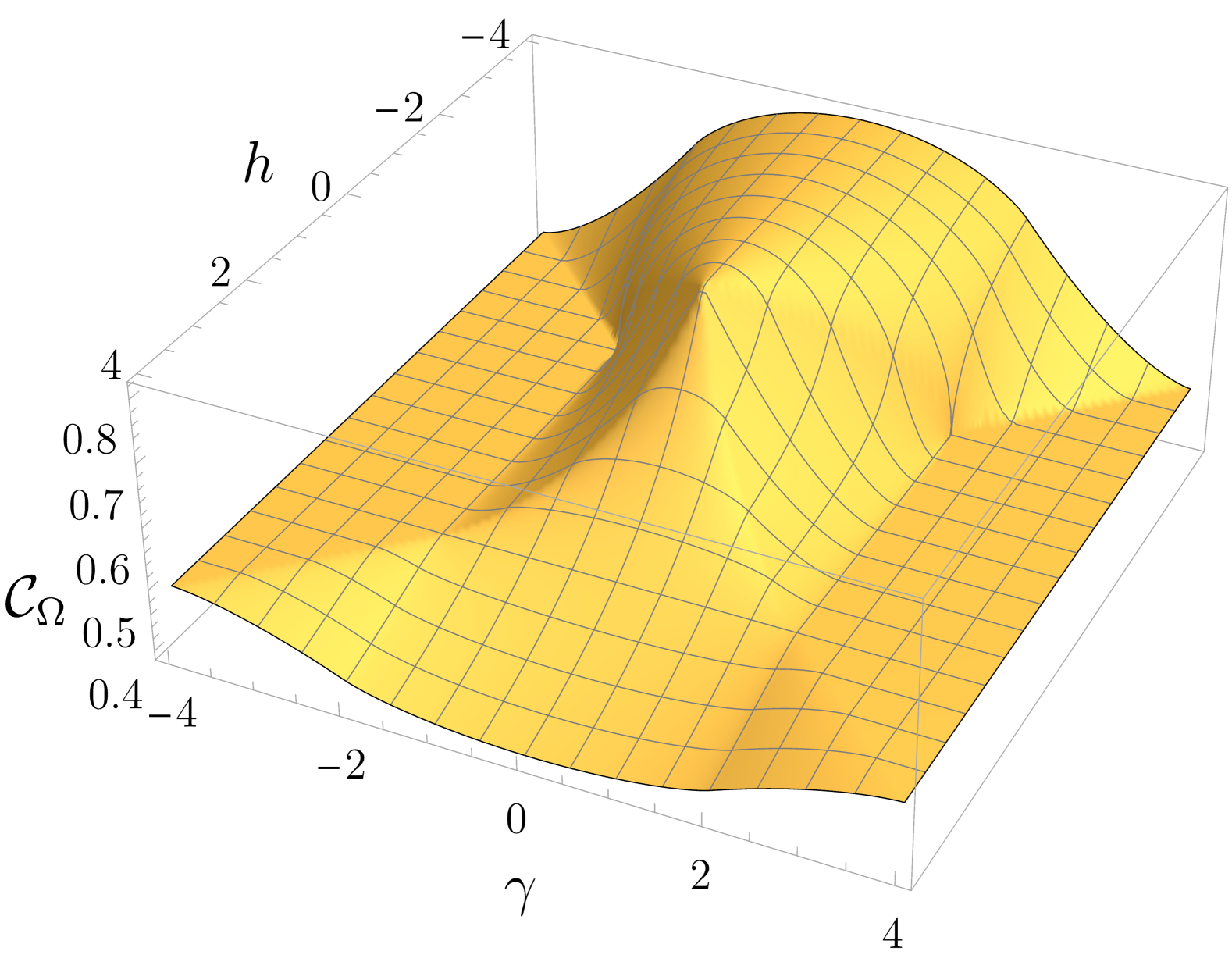
((a))

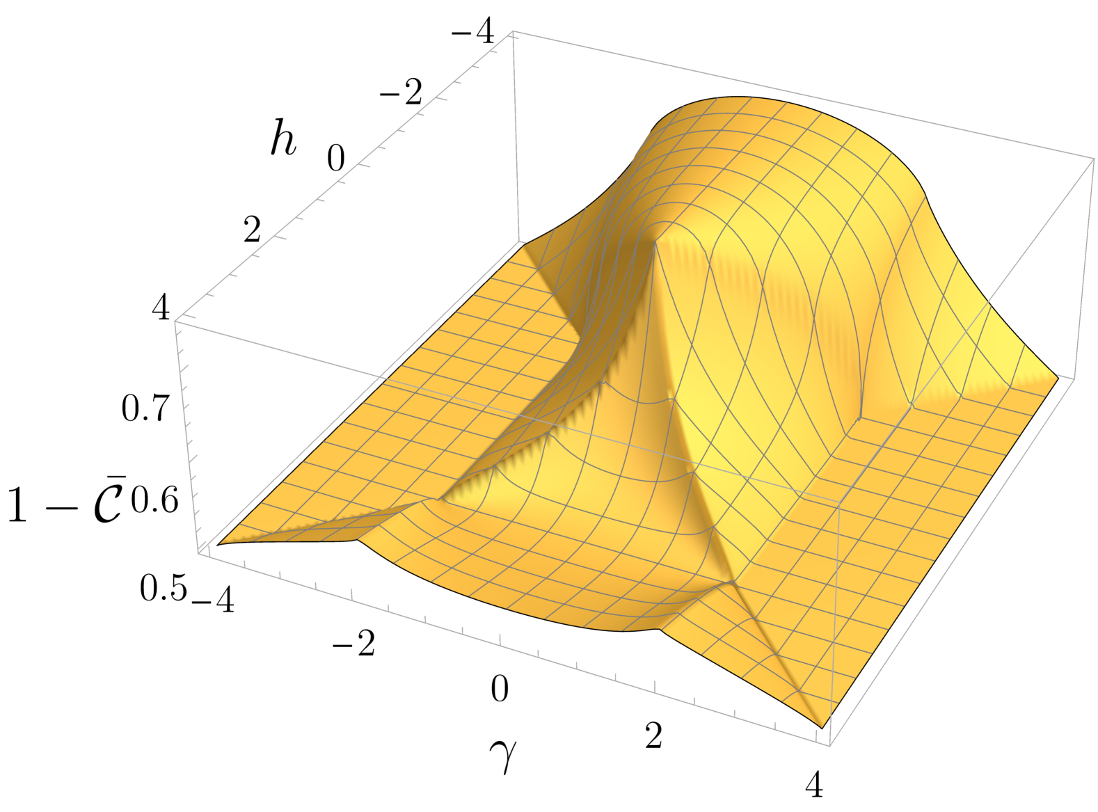
((b))

Figure 2: (a) Krylov spread complexity density $\mathcal{C}_{\Omega}$ (Eq. (16b)) of the unitary evolution taking $\ket{\text{GS}}$ to $\ket{\Omega}$ at $t=1$ via the Hamiltonian Eq. (12). (b) $1-\bar{\mathcal{C}}$, where $\bar{\mathcal{C}}$ is the time-averaged Krylov spread complexity density (32) of a non-Hermitian evolution of $\ket{\text{GS}}$ induced by the non-Hermitian SSH model. In regions IV and V (see Fig. 1), the spectrum is purely imaginary, and it can have maximally two gapless points in region IV. Thus, the state $\ket{\text{GS}}$ reaches $\ket{\Omega}$ in the infinite-time limit in the non-Hermitian evolution, and the two spreads coincide in such regions, i.e., $\mathcal{C}_{\Omega}=\bar{\mathcal{C}}=1/2$.

There is no issue in regions I and II for $h=-2J$, as

$$\mathcal{C}_{\Omega}|_{h=-2J}=\frac{1}{2}+\dfrac{\sqrt{4J^{2}-\gamma^{2}}}{2\pi J}.$$

This can be shown either by taking the limit $h\rightarrow-2J$ in Eq. (17) or by setting $h=-2J$ in Eq. (16b). For regions III and VI, the value at $h=-2J$ is $1/2$. As we can see in Figs. 2(a) and 3, the spread is continuous across the domain — This seems to be a characteristic of the spread for this type of non-Hermitian systems, see, e.g., Ref. Guerra et al. (2025). However, the derivatives of $\mathcal{C}_{\Omega}$ with respect to $h$ (or $\gamma)$ display the following behavior: if we start in Region I (i.e., the $\mathcal{PT}$-symmetric phase) with $h=-2J$, (see Fig. 3b in red), the first derivative with respect to $\gamma$ is

$$\left(\partialderivative{\mathcal{C}_{\Omega}|_{h=-2J}}{\gamma}\right)_{\text{I}}=-\dfrac{\gamma}{2J\pi\sqrt{4J^{2}-\gamma^{2}}},$$ (18)

and it diverges at $\absolutevalue{\gamma}=2J$. For any other point of Region I with $h\neq-2J$, the second derivative with respect to $\gamma$ is

$$\left(\partialderivative[2]{\mathcal{C}_{\Omega}}{\gamma}\right)_{\text{I}}=\dfrac{1}{\pi(h+2J)}\left(\dfrac{1}{\sqrt{4J^{2}-\gamma^{2}}}-\frac{1}{\sqrt{h^{2}-\gamma^{2}}}\right),$$ (19)

and it diverges as Region II is approached. Furthermore, starting with $\gamma=0$ (see Fig. 3a in green), which corresponds to the Hermitian case, the spread is

$$\left(\mathcal{C}_{\Omega}|_{\gamma=0}\right)_{\text{I}}=\dfrac{1}{2}-\dfrac{\absolutevalue{h}-2J}{\pi(h+2J)}.$$ (20)

and it is equal to $1/2+1/\pi$ for $h<0$. This phase corresponds to a non-trivial topological phase of the Hermitian SSH model, where the circle $(R_{x}-t_{1})^{2}+R_{z}^{2}=t_{2}^{2}$ (see Eq. (34)) encloses the origin. Thus, the index is non-zero as $k$ varies in $[-\pi,\pi)$ Araújo and Sacramento (2021). Remark that Eq. (16) of Ref. Caputa and Liu (2022) yields a value of $1/2-1/\pi$ in the same phase. This discrepancy is due to the sign in the matrix exponential in Eq. (2); that is, if $\sigma_{x}\rightarrow-\sigma_{x}$, we would recover that result.

Starting in Region III, the second derivative with respect to $\gamma$ is

$$\left(\partialderivative[2]{\mathcal{C}_{\Omega}}{\gamma}\right)_{\text{III}}=-\dfrac{1}{\pi(h+2J)}\dfrac{1}{\sqrt{h^{2}-\gamma^{2}}}.$$ (21)

Note that there is no divergence as we approach Region II, yet there is a divergent behavior as we approach Region V. Clearly, if we start in Region V, $(C_{\Omega})_{\text{V}}=1/2$, and there is no divergence as we approach Region IV. Finally, if we start in Region VI, we have

$$\left(\partialderivative{\mathcal{C}_{\Omega}}{\gamma}\right)_{\text{VI}}=-\dfrac{1}{\pi(h+2J)}\arccot\dfrac{\gamma}{\sqrt{4J^{2}-\gamma^{2}}}.$$ (22)

For $h=0$, this derivative is discontinuous at $\gamma=0$. The second derivative gives

$$\left(\partialderivative[2]{\mathcal{C}_{\Omega}}{\gamma}\right)_{\text{VI}}=\dfrac{1}{\pi(h+2J)}\dfrac{1}{\sqrt{4J^{2}-\gamma^{2}}},$$ (23)

and it starts diverging only when we approach Region IV.

We point out that the derivatives with respect to $h$ also display either discontinuities or divergences across the phase diagram. This can be seen directly from $\mathcal{C}_{\Omega}$ displayed in Figs 2(a) and 3.

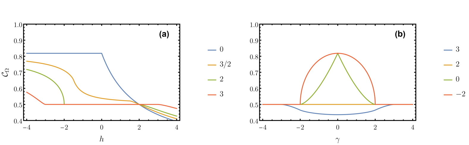
Figure 3: Transverse sections of the spread Eq. (17). (a) Spread as a function of $h$ for $\gamma\in\{0,3/2,2,3\}$. (b) Spread as a function of $\gamma$ for $h\in\{-2,0,2,3\}$. In all cases, $J=1$.

V Time-dependent Krylov spread and dynamical phase transitions

In this section, we calculate the Krylov spread of the evolution of $\ket{\psi(0)}=\ket{\text{GS}}$ via the non-Hermitian Hamiltonian $H$ in the $\mathcal{PT}$-broken phase where its spectrum is purely imaginary and gapped, i.e., $\Lambda(k)=i\Gamma(k)\neq 0\,\forall k\in\mathcal{K}$, and find $\mathcal{C}(t)\rightarrow(\mathcal{C}_{\Omega})_{V}=1/2$ as $t\rightarrow\infty$. We also implement the Krylov fidelity introduced in Ref. Guerra et al. (2025) to identify dynamical phases based on how the time-dependent Krylov spread reaches its infinite-time limit. We close the section by providing some comments about the relation between the above spread and the one in the previous section.

The reason to consider the above-mentioned particular initial state is that (see Appendix B),

$$\ket{\psi(t\rightarrow\infty)} =\lim_{t\to\infty}\dfrac{e^{-iHt}\ket{\text{GS}}}{\norm{e^{-iHt}\ket{\text{GS}}}}$$ (24a)

$$=\prod_{\begin{subarray}{c}k>0\\ s=\pm\end{subarray}}\dfrac{\exp[x_{s}(k)J_{+}^{s}(k)]}{\sqrt{1+\absolutevalue{x_{s}(k)}^{2}}}\ket{\text{GS}},$$ (24b)

where

$$x_{\pm}(k)\coloneqq\dfrac{R_{x}\mp iR_{y}}{R_{z}-i\Gamma(k)},$$ (25)

is also a coherent state of $\ket{\text{GS}}$ and is related to $\ket{\Omega}$ via the unitary operator

$$\hat{O}_{z}\coloneqq\prod_{\begin{subarray}{c}k>0\\ s=\pm\end{subarray}}\exp(2i\phi_{k}J_{z}^{s}(k)+2\phi_{k})$$ (26)

belonging to the isotropy group of $\ket{\text{GS}}$, $\text{U}(1)^{\otimes L}$, where $\phi_{k}=\text{Arg}\,[R_{z}+i\Gamma(k)]$. Specifically,

$$\ket{\psi(t\rightarrow\infty)}=\hat{O}_{z}\ket{\Omega}=\hat{\Omega}\ket{\text{GS}}=\ket*{\hat{\Omega}},$$

where $\hat{\Omega}=\hat{O}_{z}\Omega\hat{O}_{z}^{\dagger}\in\text{SU}(2)^{\otimes L}/\text{U}(1)^{\otimes L}$. Therefore, since both $\ket{\Omega}$ and $\ket*{\hat{\Omega}}$ are generalized coherent states of $\ket{\text{GS}}$, we can assert that time-dependent spread density of Eq. (24) before taking the limit is

$$\mathcal{C}(t)=\sum_{s=\pm}\int_{0}^{\pi}\dfrac{\differential k}{2\pi}\dfrac{\absolutevalue{A_{+}^{s}(k;t)}^{2}}{1+\absolutevalue{A_{+}^{s}(k;t)}^{2}},$$ (27)

and it tends to $1/2$ as $t\rightarrow\infty$ when $\Lambda(k)=i\Gamma(k)$. Note that this is precisely $\left(\mathcal{C}_{\Omega}\right)_{\text{V}}=1/2$, so the spread of $\ket{\psi(t)}$, as it evolves from $\ket{\text{GS}}$ to $\ket*{\hat{\Omega}}$ via $H$ with a purely imaginary spectrum, is the same as the spread of the same initial state evolving to $\ket{\Omega}$ via the Hermitian Hamiltonian (12).

Given Eq. (27), we can characterize how $\mathcal{C}(t)$ reaches $(\mathcal{C}_{\Omega})_{\text{V}}=1/2$ with the Krylov spread fidelity Guerra et al. (2025)

$$\mathcal{F}(t)=\absolutevalue{\mathcal{C}(t)-\mathcal{C}_{\Omega}}$$ (28)

by requiring $\mathcal{F}(t)<\epsilon<1$ and then finding the time $t(\epsilon)$ for which the inequality holds. Hence, we denote $\mathcal{C}_{\text{st}}(t)=\mathcal{C}(t>t(\epsilon))\simeq\mathcal{C}_{\Omega}$ as the stationary state spread. Once $t(\epsilon)$ is found, we find the limit

$$t^{*}=\lim_{\epsilon\to 0}\dfrac{t(\epsilon)}{\absolutevalue{\ln\epsilon}}$$ (29)

to obtain an $\epsilon$-independent description, which serves two things: it defines the stationary state for times $t\gg t*$, and it serves as a probe for detecting dynamical phase transitions. By following this description, we find that $t^{*}$ attains two values (see Appendix C):

$$t_{1}(\epsilon) \simeq\dfrac{1}{4\sqrt{\gamma^{2}-4J^{2}}}W_{0}\left(\frac{4(\gamma^{2}-4J^{2})^{3}}{\epsilon^{2}\pi\gamma^{4}(4J^{2}-h^{2})}\right)\ \underbrace{\rightarrow}_{\epsilon\to 0}\ \dfrac{1}{2\sqrt{\gamma^{2}-4J^{2}}}\ln\dfrac{1}{\epsilon},\qquad t^{*}_{1}=\dfrac{1}{2\sqrt{\gamma^{2}-4J^{2}}},$$ (30)

$$t_{2}(\epsilon) \simeq\dfrac{1}{4\sqrt{\gamma^{2}-h^{2}}}W_{0}\left(\frac{4(\gamma^{2}-h^{2})^{3}}{\epsilon^{2}\pi\gamma^{4}(h^{2}-4J^{2})}\right)\ \underbrace{\rightarrow}_{\epsilon\to 0}\ \dfrac{1}{2\sqrt{\gamma^{2}-h^{2}}}\ln\dfrac{1}{\epsilon},\qquad t^{*}_{2}=\dfrac{1}{2\sqrt{\gamma^{2}-h^{2}}},$$ (31)

where $W_{0}(z)$ is the Lambert $W$ function, which has the asymptotics $W_{0}(z\rightarrow\infty)\simeq\ln z-\ln(\ln z).$ These times refine Region V as shown in Fig. 4, where $t_{1}^{*}$ corresponds to $\{\absolutevalue{h}\leq 2J,\absolutevalue{\gamma}>2J\}$ and $t_{2}^{*}$ corresponds to $\{\absolutevalue{h}\geq 2J,\absolutevalue{\gamma}>h\}$. Qualitatively, the change in the time $t^{*}$ from region 1 to 2 is due to the location of the slowest dissipation mode of $\Lambda(k)=i\Gamma(k)$: in Region 1, $\absolutevalue{\Gamma(0)}=0$, whereas in Region 2, $\absolutevalue{\Gamma(\pi)}=0$. This can be seen in Fig. 1b-d in the purple, dotted lines. Due to this change in the slowest dissipation mode as Region V is traversed, the first derivative of $t^{*}$ with respect to $h$ is discontinuous, indicating thus the presence of the dynamical phase transition.

Let us consider the other regions where the spectrum can have a non-vanishing real part. To address this, we consider the time-average of the spread density

$$\bar{\mathcal{C}}=\lim_{T\to\infty}\dfrac{1}{T}\int_{0}^{T}\differential t\,\mathcal{C}(t),$$ (32)

where $\mathcal{C}(t)$ is as in Eq. (27). The order of the limits in Eq. (32) can be interchanged as the integrand of $\mathcal{C}(t)$ is well-behaved (see Appendix D). Now, in regions III and IV, where the spectrum is complex, one could naively expect that $\bar{\mathcal{C}}=\mathcal{C}_{\Omega}$, where the latter spread is given by Eq. (17). However, this does not hold due to the continuum of imaginary gapless modes appearing whenever $E(k)\neq 0$. The above equality holds in the non-Hermitian Ising model studied in Ref. Guerra et al. (2025) due to the presence of only two gapless modes in the imaginary part of the spectrum. Hence, as an educated guess, $\bar{\mathcal{C}}=\mathcal{C}_{\Omega}$ holds only when there is a finite number of gapless modes in the imaginary part of the spectrum. This can be seen in in Fig. 2(b) were we show $1-\bar{\mathcal{C}}$. In Region V, where the spectrum is imaginary and can have at most two gapless modes, the two spreads match and equal $1/2$. In the remaining regions, the spreads do not coincide (see Fig. 2(a)). However, this averaged spread could also serve as a probe for the phase transitions we explored before with $\mathcal{C}_{\Omega}$, as the boundaries corresponding to regions II and IV are not smooth. The overall resemblance of $1-\bar{\mathcal{C}}$ and $\mathcal{C}_{\Omega}$ requires further research.

Figure 4: Schematic phase diagram defined via the Krylov fidelity (28) with $J=1$. Region 1 (in gray) corresponds to the time (30), and Region 2 (in light blue) corresponds to the time (31). The points in red correspond to Region IV (see Fig. 1), where $\Lambda(k)=i\Gamma(k)=0$, so we do not associate any $t^{*}$ with those points. The white regions correspond to the points where the spectrum is either purely or partially real, so there is no $t^{*}$ as well for such points.

VI Summary and discussion

In this work, we implemented the Krylov spread density as a probe to detect a $\mathcal{PT}$-symmetry breaking in a non-Hermitian SSH model, where the spectrum goes from real to complex, and another spectral transition when the spectrum goes from complex to imaginary. In the $\mathcal{PT}$-broken phase, where the spectrum is imaginary, we used the Krylov fidelity to determine how the spread reaches its stationary state limit and found two characteristic times that define two dynamical phases.

As we saw in Sec. III, the spread depends on the initial state and the generator of the dynamics. Therefore, different initial states can yield different spreads for the same Hamiltonian. Hence, since we aimed to study the non-Hermitian vacuum $\ket{\Omega}$ of the non-Hermitian SSH Hamiltonian (1), we chose an appropriate initial state $\ket{\psi(0)}=\ket{\text{GS}}$ (Eq. (14)) for which $\ket{\Omega}=\Omega\ket{\text{GS}}$ (Eq. (15)) is a generalized coherent state. Thanks to this relation, we could find the Hermitian Hamiltonian (12) inducing the evolution of $\ket{\psi(0)}$ to $\ket{\Omega}$ at $t=1$. We calculated the spread density $\mathcal{C}_{\Omega}$ (Eq. (17)) of this evolution when the non-Hermitian vacuum was reached. The first important conclusion is the lack of symmetry in $\mathcal{C}_{\Omega}$ with respect to the reflection of the parameters $(h,\gamma)\rightarrow(-h,-\gamma)$ (see Fig. 2(a)). In contrast, the spectrum (6) is symmetric with respect to this reflection (see also Fig. 1). Secondly, even though $\mathcal{C}_{\Omega}$ is continuous across the $h$-$\gamma$ plane, its first and second derivatives with respect to $\gamma$ and $h$ are either discontinuous or diverge when $\mathcal{PT}$-symmetry breaks (Eqs. (18)-(19)) and where the spectrum becomes purely imaginary (Eqs. (21)-(23)). With this, we can assert the usefulness of the spread as a probe for detecting phase transitions in general.

The other spread we considered was of the same initial state $\ket{\text{GS}}$, but this time evolving under the SSH Hamiltonian. In the $\mathcal{PT}$-broken phase corresponding to an imaginary spectrum, $\ket{\text{GS}}$ evolves to $\ket{\Omega}$ in the infinite-time limit, proving, thus, the importance of that particular initial state as it is related to the vacuum of $H$ in two different ways. Since the same state is reached via the unitary dynamics mentioned before, the time-dependent spread (27) of the non-Hermitian dynamics tends to $\mathcal{C}_{\Omega}$ in the infinite-time limit. By implementing the Krylov fidelity (28) to study how $\mathcal{C}(t)$ approaches $\mathcal{C}_{\Omega}$ in this region of the $\mathcal{PT}$-broken phase where the spectrum is imaginary, we were able to determine two times, Eqs.(30) and (31), characterizing two previously unknown dynamical phases existing in this subregion. Interestingly, in this subregion, $\mathcal{C}(t\rightarrow\infty)=\mathcal{C}_{\Omega}$ is constant and the entanglement entropy calculated in the $\ket{\Omega}$ same state obeys an area law Gal et al. (2023). However, having a constant spread does not imply that the entanglement entropy obeys an area law. In Fig. 3, we can see a constant spread for $h<0$ and $\gamma=0$, where the $\mathcal{PT}$-symmetry is unbroken. In this phase, the entanglement entropy obeys a volume law. Also, in Ref. Guerra et al. (2025), it was shown that the spread of a non-Hermitian Ising chain is not constant in the region where the entanglement entropy calculated in its vacuum obeys an area law Zerba and Silva (2023). Additional research is needed to understand the relationship between these two quantities better

We calculated the time-averaged spread (32) in the regions where the spectrum is complex. We found that $\bar{\mathcal{C}}\neq\mathcal{C}_{\Omega}$ except for the region where the spectrum is imaginary. This should be of no surprise, as the non-Hermitian SSH model we treated has the peculiarity of having either a real or imaginary spectrum per each momentum mode $k$. Thus, the absence of those dissipation modes whenever the real part is non-zero impedes the convergence of $\ket{\text{GS}}$ to $\ket{\Omega}$, which translates into a different spread even after performing a time-averaging. Nonetheless, $\bar{\mathcal{C}}$ is qualitatively similar (see Fig. 2) to $\mathcal{C}_{\Omega}$ throughout the $h$-$\gamma$ plane. Therefore, either spread can be used as a probe to detect the phase transitions we described above. However, as the time-averaging produced a quite complicated function in $k$, we were unable to find an analytic expression for $\bar{\mathcal{C}}$, so $\mathcal{C}_{\Omega}$ is perhaps more convenient.

The conjecture stated in Ref. Guerra et al. (2025), where it was stated that the derivatives of the Krylov spread diverge across any quantum phase transitions, was also corroborated for the model here treated. Naturally, as a formal proof is worth pursuing, a tour de-Force can be used to verify this for many other phase transitions such as, e.g., measurement-induced and $\mathcal{PT}$-transitions. In addition, we studied the Krylov spread only in the left eigenbasis of the non-Hermitian Hamiltonian, and it would be reasonable to study this measure on the left and right basis, i.e., by using a bi-orthogonal approach. Also, as in the Hermitian SSH model, the spread is constant in the non-trivial topological phase (see Eq. (20) and Ref. Caputa and Liu (2022)), it is worth researching the relation, if any, between topological phases and the spread for the non-Hermitian SSH model we treated and further generalizations Nair et al. (2023); Lieu (2018b); Wong et al. (2024); He and Chien (2020); Nehra and Roy (2022); Rottoli et al. (2024); Zhou (2024). In addition, the study of the non-Hermitian SSH model with several quenches Gautam et al. (2024) can also be investigated.

Importantly, while finalizing this manuscript, Ref. Chakrabarti et al. (2025) was posted, where the dynamics of the same non-Hermitian SSH model with periodic and open boundary conditions were analyzed in Krylov space by implementing numeric methods, and a very particular state: a particle localized on the 15th site of the lattice. The authors were able to detect the $\mathcal{PT}$-transition in the time-dependent Krylov spread calculated via the bi-Lanczos algorithm. However, Ref. Chakrabarti et al. (2025) had to go beyond standard Krylov methods and utilized the quantum Fisher information in Krylov space to detect the complex-to-imaginary spectral transition. In contrast, in our work, all these phase transitions were identified by means of the Krylov spread density on an equal footing based on the analytical solution using a canonical state. Moreover, we disclosed previously hidden dynamical phase transitions using the same Krylov framework.

VII Acknowledgments

Y.G. was supported by the Deutsche Forschungsgemeinschaft (DFG, German Research Foundation) grant SH 81/8-1 and by a National Science Foundation (NSF)–Binational Science Foundation (BSF) grant 2023666.

Appendix A Diagonalization of $H$ and the non-Hermitian Bogoliubov vacuum

In this appendix, we diagonalize the non-Hermitian Hamiltonian  (1) by implementing the Fourier representation (2) and find the eigenvalues (6) as well as the ground state (15). We also demonstrate that this ground state is a generalized coherent state of the ground state (11).

After using the Fourier representation (2), the Hamiltonian can be written as $H=\sum_{k}H(k)$, where

$$H(k)=\begin{pmatrix}c_{k}^{\dagger}&d_{k}^{\dagger}\end{pmatrix}\begin{pmatrix}t_{2}\sin k&t_{1}+t_{2}\cos k+t_{2}-\gamma\\ t_{1}+t_{2}\cos k+\gamma&-t_{2}\sin k\end{pmatrix}\begin{pmatrix}c_{k}\\ d_{k}\end{pmatrix}.$$ (33)

Alternatively, depending on our needs, we can set $H(k)\equiv\Psi_{k}^{\dagger}\vec{R}(k)\cdot\vec{\sigma}\,\Psi_{k}$, where $\Psi_{k}=(c_{k},d_{k})^{T}$,

$$\vec{R}(k)=\begin{pmatrix}R_{x}\\ R_{y}\\ R_{z}\end{pmatrix}=\begin{pmatrix}t_{1}+t_{2}\cos k\\ -i\gamma\\ t_{2}\sin k\end{pmatrix}$$ (34)

is a complex Bloch vector, and $\vec{\sigma}=(\sigma_{x},\sigma_{y},\sigma_{z})$ is a vector of Pauli matrices. Recall that

$$t_{1}=-J-\frac{h}{2},\,\,t_{2}=-J+\frac{h}{2}.$$

The matrix $\vec{R}(k)\cdot\vec{\sigma}$ can be diagonalized by a similarity transformation as $V_{k}^{-1}\vec{R}(k)\cdot\vec{\,}\sigma V_{k}=\text{diag}\left[\Lambda(k),-\Lambda(k)\right]$, where

$$V_{k}=\begin{pmatrix}u_{k}&u_{k}\\ v_{k}^{+}&v_{k}^{-}\end{pmatrix}\equiv\begin{pmatrix}\vec{v}_{+}(k)&\vec{v}_{-}(k)\end{pmatrix},$$ (35)

and

$$\vec{v}_{\pm}(k)=\dfrac{1}{\sqrt{2R(R\mp R_{z})}}\begin{pmatrix}R_{x}-iR_{y}\\ \pm R-R_{z}\end{pmatrix}.$$ (36)

Here, $R=\Lambda(k)$ is the positive root given by Eq. (6).

Thanks to the similarity transformation, we can define the following non-Hermitian fermionic operators

$$X_{k}^{*}=\begin{pmatrix}\chi_{+,k}^{*}&\chi_{-,k}^{*}\end{pmatrix}\coloneqq\Psi_{k}^{\dagger}V_{k}=\begin{pmatrix}u_{k}c_{k}^{\dagger}+v_{k}^{+}d_{k}^{\dagger}&u_{k}c_{k}^{\dagger}+v_{k}^{-}d_{k}^{\dagger}\end{pmatrix}$$ (37)

and

$$X_{k}=\begin{pmatrix}\chi_{+,k}\\ \chi_{-,k}\end{pmatrix}\coloneqq V_{k}^{-1}\Psi_{k}=\dfrac{1}{\det V_{k}}\begin{pmatrix}v_{k}^{-}c_{k}-u_{k}d_{k}\\ -v_{k}^{+}c_{k}+u_{k}d_{k}.\end{pmatrix},$$ (38)

which satisfy the anticommutation relations (5). Given these new fermionic operators, we can write the Hamiltonian as in Eq. (4)

Akin to the Hermitian version of Eq. (1), the unnormalized ground state of $H$ (cf. Eq. (15)), which is a non-Hermitian Bogoliubov vacuum, is obtained by populating the vacuum $\ket{0}$, which is annihilated by $c_{k}$ and $d_{k}$, by the non-Hermitian quasiparticles associated to a negative complex spectrum, i.e.,

$$\ket*{\tilde{\Omega}}=\prod_{k\in\mathcal{K}^{+}}\chi_{-,-k}^{*}\chi_{-,k}^{*}\ket{0},$$ (39)

where $\mathcal{K}^{+}=\mathcal{K}\cap\mathbb{R}_{\geq 0}.$ Thus, $H\ket*{\tilde{\Omega}}=E_{\Omega}\ket*{\tilde{\Omega}}$, and so the ground state energy is

$$E_{\Omega}=-\sum_{k\in\mathcal{K}^{+}}\Lambda(k).$$ (40)

This is a natural choice of the sign of the spectrum for each $k$, for whenever $\mathfrak{Im}\,\Lambda(k)=\Gamma(k)\neq 0$, $\ket*{\tilde{\Omega}}$ decays the slowest. Further, if $\Gamma(k)=0$, then $\Lambda(k)=E(k)<0$ is a real number, and Eq. (39) is the state with the lowest energy in the given still non-Hermitian system.

To demonstrate that $\ket{\Omega}=\norm*{\ket*{\tilde{\Omega}}}^{-1/2}\ket*{\tilde{\Omega}}$ a generalized coherent state of Eq. (14), which is the ground state of Eq. (11), let us consider the non-Hermitian Hamiltonian once more:

$$H =\sum_{k\in\mathcal{K}^{+}}\left[R_{z}(k)\left(c_{k}^{\dagger}c_{k}-d_{k}^{\dagger}d_{k}\right)+R_{+}c_{k}^{\dagger}d_{k}+R_{-}d_{k}^{\dagger}c_{k}-R_{z}(k)\left(c_{-k}^{\dagger}c_{-k}-d_{-k}^{\dagger}d_{-k}\right)+R_{+}c_{-k}^{\dagger}d_{-k}+R_{-}d_{-k}^{\dagger}c_{-k}\right],$$ (41)

where we used $R_{z}(-k)=-R_{z}(k)$ and set $R_{+}(k)=R_{x}(k)-iR_{y}(k)$ and $R_{-}(k)=R_{x}(k)+iR_{y}(k)$. Contrary to the Hermitian case, $R_{+}^{*}\neq R_{-}$. In this form, $H$ can be seen as an element of the semisimple Lie algebra $\mathfrak{g}=\mathfrak{g}^{+}\times\mathfrak{g}^{-}=\mathfrak{su}(2)\times\mathfrak{su}(2)$. More precisely, if we set

$$J^{+}_{+}(k)\coloneqq c_{k}^{\dagger}d_{k},\quad J_{-}^{+}(k)\coloneqq d_{k}^{\dagger}c_{k},\quad J_{z}^{+}(k)\coloneqq\dfrac{1}{2}\left(c_{k}^{\dagger}c_{k}-d_{k}^{\dagger}d_{k}\right),$$ (42)

and

$$J^{-}_{+}(k)\coloneqq d_{-k}^{\dagger}c_{-k},\quad J_{-}^{-}(k)\coloneqq c_{-k}^{\dagger}d_{-k},\quad J_{z}^{-}(k)\coloneqq-\dfrac{1}{2}\left(c_{-k}^{\dagger}c_{-k}-d_{-k}^{\dagger}d_{-k}\right),$$ (43)

it holds that

$$[J_{+}^{s}(k),J_{-}^{s^{\prime}}(k^{\prime})]=2\delta_{ss^{\prime}}\delta_{k,k^{\prime}}J_{z}^{s}(k),\quad[J_{z}^{s}(k),J_{\pm}^{s^{\prime}}(k^{\prime})]=\pm\delta_{ss^{\prime}}\delta_{kk^{\prime}}J_{\pm}^{s}(k),$$ (44)

where $s,s^{\prime}=\pm$. The superindices denote which Lie algebra the element belongs to, and the subindices denote the generator in the given Lie algebra. Thus, Eq. (41) can be rewritten as

$$H=\sum_{\begin{subarray}{c}k\in\mathcal{K}^{+}\\ s=\pm\end{subarray}}H^{(s)}(k),$$ (45)

where $H^{(s)}(k)=2R_{z}(k)J_{z}^{s}(k)+R_{+}^{s}(k)J_{+}^{s}(k)+R_{-}^{s}(k)J_{-}(k)$. Note that $R^{+}_{+}=R_{-}^{-}=R_{+}$ and $R^{+}_{-}=R_{+}^{-}=R_{-}$.

Given this Lie-algebraic language, and by noting that $J_{-}^{\pm}(k)\ket{\text{GS}}=0$, we can identify $\ket{\text{GS}}$ with the lowest-weight state of $\mathfrak{g}$,

$$\ket{\text{GS}}=\prod_{k\in\mathcal{K}^{+}}c_{-k}^{\dagger}d_{k}^{\dagger}\ket{0}=\bigotimes_{k\in\mathcal{K}}\ket{1/2,-1/2}_{k},$$ (46)

where $J_{-}^{\pm}(k)\ket{1/2,-1/2}_{\pm k}=0$, $J_{+}^{\pm}(k)\ket{1/2,-1/2}_{\pm k}=\ket{1/2,1/2}_{\pm k}$, and $J_{z}^{\pm}(k)\ket{1/2,\pm 1/2}_{\pm k}=\pm\frac{1}{2}\ket{1/2,\pm 1/2}_{\pm k}$. Moving forward, by noticing that $[J^{\pm}_{+}(k),c_{-k^{\prime}}^{\dagger}d_{k^{\prime}}^{\dagger}]=0$ for $k\neq k^{\prime}$, we can analyze the action of $J_{\pm}^{\pm}(k)$ on $\ket{\text{GS}}$ by focusing on the following states:

$$J_{+}^{+}(k)c_{-k}^{\dagger}d_{k}^{\dagger}\ket{0} =c_{-k}^{\dagger}c_{k}^{\dagger}\ket{0},$$ (47)

$$J_{+}^{-}(k)c_{-k}^{\dagger}d_{k}^{\dagger}\ket{0} =d_{-k}^{\dagger}d_{k}^{\dagger}\ket{0},$$ (48)

and

$$J_{+}^{+}(k)J_{+}^{-}(k)\ket{0}=d_{-k}^{\dagger}c_{k}^{\dagger}\ket{0}.$$ (49)

Now, for $y_{\pm}(k)\in\mathbb{C}$ and $k\in\mathcal{K}^{+}$, let

$$\tilde{\Omega}_{k}\coloneqq\exp[y_{+}(k)J^{+}_{+}(k)+y_{-}(k)J_{+}^{-}(k)]$$ (50)

and consider

$$\tilde{\Omega}_{k}\,c_{-k}^{\dagger}d_{k}^{\dagger}\ket{0}=\exp[y_{+}(k)J_{+}^{+}(k)+y_{-}(k)J_{+}^{-}(k)]c_{-k}^{\dagger}d_{k}^{\dagger}\ket{0}=\left(c_{-k}^{\dagger}d_{k}^{\dagger}+y_{+}c_{-k}^{\dagger}c_{k}^{\dagger}+y_{-}d_{-k}^{\dagger}d_{k}^{\dagger}+y_{+}y_{-}d_{-k}^{\dagger}c_{k}^{\dagger}\right)\ket{0}.$$ (51)

On the other hand, by expanding Eq. (39), we get

$$\ket*{\tilde{\Omega}}=\prod_{k\in\mathcal{K}^{+}}u_{-k}v_{k}^{-}\left(c_{-k}^{\dagger}d_{k}^{\dagger}+\dfrac{u_{k}}{v_{k}^{-}}c_{-k}^{\dagger}c_{k}^{\dagger}+\dfrac{v_{-k}^{-}}{u_{-k}}d^{\dagger}_{-k}d_{k}^{\dagger}+\dfrac{u_{k}v_{-k}^{-}}{u_{-k}v_{k}^{-}}d_{-k}^{\dagger}c_{k}^{\dagger}\right)\ket{0}.$$ (52)

Hence, if we set

$$y_{+}(k)=\dfrac{u_{k}}{v_{k}^{-}}\quad\text{and}\quad y_{-}(k)=\dfrac{v_{-k}^{-}}{u_{-k}}$$ (53)

we can write Eq. (52) as

$$\ket*{\tilde{\Omega}}=\prod_{k\in\mathcal{K}^{+}}u_{-k}v_{k}^{-}\exp(\dfrac{u_{k}}{v_{k}^{-}}J_{+}^{+}(k)+\dfrac{v_{-k}^{-}}{u_{-k}}J_{+}^{-}(k))\ket{\text{GS}},$$ (54)

and, after normalizing, it reads

$$\ket{\Omega}=\prod_{k\in\mathcal{K}^{+}}\dfrac{u_{-k}v_{k}^{-}}{\absolutevalue{u_{-k}v_{k}^{-}}}\dfrac{\exp[y_{+}(k)J^{+}_{+}(k)+y_{-}(k)J_{+}^{-}(k)]}{\left(1+\absolutevalue{y_{+}(k)}^{2}\right)^{1/2}\left(1+\absolutevalue{y_{-}(k)}^{2}\right)^{1/2}}\ket{\text{GS}}.$$ (55)

As our final step, let $\alpha_{z},\alpha_{\pm}\in\mathbb{C}$, and $J_{\pm},J_{z}\in\mathfrak{su}(2)$, and consider the normal-ordering $\mathfrak{su}(2)$ decomposition formula Ban (1993)

$$\exp(a_{+}J_{+}+a_{z}J_{z}+a_{-}J_{-})=\exp(\alpha_{+}J_{+})\exp[\log(\alpha_{z})J_{z}]\exp(\alpha_{-}J_{-}),$$ (56)

where

$$\alpha_{\pm}=\dfrac{a_{\pm}}{\phi}\dfrac{\sinh\phi}{\cosh\phi-\dfrac{a_{z}}{2\phi}\sinh\phi},\quad\alpha_{z}=\left[\cosh\phi-\dfrac{a_{z}}{2\phi}\sinh\phi\right]^{-2},\quad\phi=\sqrt{\dfrac{a_{z}^{2}}{4}+a_{+}a_{-}},$$ (57)

applied to the following unitary operators

$$\Omega_{k}^{+}\coloneqq\exp[y_{+}(k)J_{+}^{+}(k)-\text{H.c}],\quad\text{and}\quad\Omega_{k}^{-}\coloneqq\exp[y_{-}(k)J_{+}^{-}(k)-\text{H.c}]$$ (58)

acting on $\ket{1/2,-1/2}_{k}$ and $\ket{1/2,-1/2}_{-k}$, respectively. Upon applying those steps and some simple algebraic manipulations, we get

$$\Omega_{k}^{\pm}\ket{1/2,-1/2}_{\pm k} =\dfrac{\exp[y_{\pm}(k)J_{+}^{\pm}(k)]}{\sqrt{1+\absolutevalue{y_{\pm}(k)}^{2}}}\ket{1/2,-1/2}_{\pm k}.$$ (59)

Thus, by calling $\Omega\coloneqq\Omega_{k}^{+}\Omega_{k}^{-}$ and $\exp[i\varphi(\Omega)]\coloneqq\prod_{k\in\mathcal{K}^{+}}u_{-k}v_{k}^{-}/\absolutevalue{u_{-k}v_{k}^{-}}$, we can immediately conclude that Eq. (55) is equal to

$$\ket{\Omega}=\exp[i\varphi(\Omega)]\Omega\ket{\text{GS}}.$$ (60)

Finally, by noting that the action of operators of the form $\exp[a_{z}^{+}J_{z}^{+}(k)+a_{z}^{-}J_{z}^{-}(k)]$ on $\ket{\text{GS}}$ only produces a phase, we can conclude that $\ket{\Omega}$ is a generalized coherent state of $\ket{\text{GS}}$ defined in the coset space $\text{SU}(2)^{\otimes L}/\text{U}(1)^{\otimes L}$ Perelomov (1986); Kam et al. (2023), and thus the phase appearing in (60) is unimportant in our analysis. Note also that the Hermitian Hamiltonian (12) used in the unitary evolution $\ket{\psi(1)}=e^{-i\hat{H}}\ket{\text{GS}}$ is obtained from $\Omega$ (see Eq. (58)).

Appendix B Time-evolution of under the non-Hermitian SSH Hamiltonian

In what follows, we find the time-evolution of the state $\ket{\text{GS}}$ induced by $H$ by invoking the same $\mathfrak{su}(2)$ decomposition formula (56) and obtain Eq. (24). To this end, let $s=\pm$ and consider

$$\exp[-iH^{s}(k)t] =\exp{-i\left[2R_{z}(k)J_{z}^{s}(k)+R_{+}^{s}(k)J_{+}^{s}(k)+R_{-}^{s}(k)J_{-}^{s}(k)\right]t}$$ (61a)

$$=\exp[A_{+}^{s}(k;t)J_{+}^{s}(k)]\exp[\ln(A_{z}^{s}(k;t))J_{z}^{s}(k)]\exp[A_{-}^{s}(k;t)J_{-}^{s}(k)],$$ (61b)

where

$$A_{\pm}^{s}(k;t) =-i\dfrac{R_{s}^{s}(k)}{\Lambda(k)}\dfrac{\sin\Lambda(k)t}{\cos\Lambda(k)t+i[R_{z}(k)/\Lambda(k)]\sin\Lambda(k)t}$$ (62)

and

$$A_{z}^{+}(k;t)=\left[\cos\Lambda(k)t+i[R_{z}(k)/\Lambda(k)]\sin\Lambda(k)t\right]^{-2}.$$ (63)

Thus, up to a phase,

$$\ket*{\psi(t)}=\dfrac{e^{-iHt}\ket{\text{GS}}}{\norm{e^{-iHt}\ket{\text{GS}}}}=\prod_{\begin{subarray}{c}k>0\\ s=\pm\end{subarray}}\dfrac{\exp[A_{+}^{s}(k;t)J_{+}(k)]}{\sqrt{1+\absolutevalue{A_{+}^{s}(k;t)}^{2}}}\ket{\text{GS}}.$$ (64)

Given this expression, let us assume that $\Lambda(k)=i\Gamma(k)\in i\mathbb{R}$, where $\Gamma(k)=\sqrt{\absolutevalue{R_{y}(k)}^{2}-R_{x}^{2}(k)-R_{z}^{2}(k)}$. Thus, we can conveniently rewrite $A_{+}^{\pm}(k;t)$ as

$$A_{+}^{\pm}(k;t)=-\dfrac{R_{x}(k)\mp iR_{y}(k)}{R_{z}(k)+i\Gamma(k)}\dfrac{1}{1-l_{k}(t)},$$ (65)

where

$$l_{k}(t)\coloneqq\frac{2}{f_{k}\left(1-\exp[-2\Gamma(k)t]\right)}$$ (66)

and $f_{k}\coloneqq 1+R_{z}(k)[i\Gamma(k)]^{-1}$. In the limit $t\rightarrow\infty$, $l_{k}(t)\rightarrow 2f_{k}^{-1}$, and $A_{+}^{\pm}(k;t)\rightarrow x_{\pm}(k)$ (see Eq. (25)). Thus, Eq. (64) yields Eq. (24b) in the limit $t\rightarrow\infty$.

Now, from Eq. (53), let us note that

$$y_{+}(k)=\dfrac{u_{k}}{v_{k}^{-}}=\dfrac{R_{x}(k)-iR_{y}(k)}{R_{z}(k)+i\Gamma(k)}\quad\text{and}\quad y_{-}(k)=\dfrac{v_{-k}^{-}}{u_{-k}}\dfrac{v_{k}^{-}}{v_{k}^{-}}=\dfrac{R_{x}(k)+iR_{y}(k)}{R_{z}(k)+i\Gamma(k)}.$$ (67)

Hence, $y_{\pm}(k)$ and $x_{\pm}(k)$ differ by a phase, implying that $\ket{\psi(t\rightarrow\infty)}$ can be related with $\ket{\Omega}$ via the unitary operator (26).

Appendix C Krylov fidelity

In this section, we outline the steps that lead to the times (30) and (31) obtained from $\mathcal{F}(t)<\epsilon$.

By expanding Eq. (28), we get

$$\mathcal{F}(t) =\absolutevalue{\int_{0}^{\pi}\dfrac{\differential k}{2\pi}\left(\dfrac{\absolutevalue{A_{+}^{+}(k;t)}^{2}}{1+\absolutevalue{A_{+}^{+}(k;t)}^{2}}-\dfrac{1}{1+\absolutevalue{A_{+}^{-}(k;t)}^{2}}\right)}.$$ (68)

Upon a few algebraic manipulations, we get

$$\absolutevalue{A_{+}^{\pm}(k;t)}^{2}=\dfrac{R_{z}^{2}(k)+\Gamma^{2}(k)}{R_{z}^{2}(k)+\Gamma^{2}(k)\coth^{2}\Gamma(k)t},$$

and, given this expression, for $\{\absolutevalue{\gamma}>2J,0<\absolutevalue{h}<2J\}$, $\absolutevalue{\Gamma(k)}$ has a minimum at $k=0$, which corresponds to the slowest decay mode, and the integrand of Eq. (68) is concentrated around this point. Hence, for sufficiently large $\Gamma(k)t$

$$\mathcal{F}(t) \approx\absolutevalue{\dfrac{\gamma^{2}-4J^{2}}{\pi\gamma^{2}}\exp(-2\sqrt{\gamma^{2}-4J^{2}}t)\int_{0}^{\infty}\differential k\,\exp[-\dfrac{4J^{2}-h^{2}}{4\sqrt{\gamma^{2}-4J^{2}}}k^{2}t]}$$

$$=\dfrac{(\gamma^{2}-4J^{2})^{5/4}}{\sqrt{\pi\,t}\,\sqrt{4J^{2}-h^{2}}\,\gamma^{2}}\exp(-2\sqrt{\gamma^{2}-4J^{2}}\,t).$$ (69)

For a given $\epsilon\in(0,1)$, we invert $\mathcal{F}(t)<\epsilon$ and get Eq. (30).

Turning to the region $\{\absolutevalue{\gamma}>\absolutevalue{h},\absolutevalue{h}>2J\}$, the minimum of $\absolutevalue{\Gamma(k)}$ shifts to $k=\pi$ and the integrand of Eq. (68) concentrates at this point. Thus, under similar steps,

$$\mathcal{F}(t) \approx\absolutevalue{\dfrac{h^{2}-\gamma^{2}}{\pi\gamma^{2}}\exp(-2\sqrt{\gamma^{2}-h^{2}}t)\int_{-\infty}^{\pi}\differential k\,\exp[\dfrac{-(h^{2}-4J^{2})}{4\sqrt{\gamma^{2}-h^{2}}}(k-\pi)^{2}t]}$$

$$=\dfrac{(\gamma^{2}-h^{2})^{5/4}}{\sqrt{\pi\,t}\sqrt{h^{2}-4J^{2}}\,\gamma^{2}}\exp(-2\sqrt{\gamma^{2}-h^{2}}\,t).$$ (70)

Once again, by fixing an $\epsilon\in(0,1)$ and setting $\mathcal{F}(t)<\epsilon$, one can invert the resulting expression to find the time (31).

Appendix D Time-averaged spread density

In this section, we demonstrate that the order of the integrals in Eq. (32) can be interchanged. Namely,

$$\lim_{T\to\infty}\dfrac{1}{T}\int_{0}^{T}\differential t\,\sum_{s=\pm}\int_{0}^{\pi}\dfrac{\differential k}{2\pi}C_{s}(k;t)=\sum_{s=\pm}\int_{0}^{\pi}\dfrac{\differential k}{2\pi}\,\lim_{T\to\infty}\int_{0}^{T}\differential t\,C_{s}(k;t).$$ (71)

Let $H$ have a purely real spectrum, i.e., $\Lambda(k)=E(k)$, which is also gapped. Then,

$$C_{s}(k;t)=\dfrac{\absolutevalue{A_{+}^{s}(k;t)}^{2}}{1+\absolutevalue{A_{+}^{s}(k;t)}^{2}}=\dfrac{\left(R_{x}(k)-s\absolutevalue{R_{y}(k)}\right)^{2}\sin^{2}E(k)t}{\left[\left(R_{x}(k)-s\absolutevalue{R_{y}(k)}\right)^{2}+R_{z}^{2}(k)\right]\sin^{2}E(k)t+E^{2}(k)\cos^{2}E(k)t}.$$

Let $T_{n}=2\pi n/E(k)$ for $n\in\mathbb{Z}^{+}$ and define the sequence of functions $\{f_{n}(k)\}_{n}$ with

$$f_{n}(k)=\frac{1}{T_{n}}\int_{0}^{T_{n}}\differential t\,\left[C_{1}(k;t)+C_{2}(k;t)\right]$$

converging to

$$f(k)=\lim_{n\to\infty}f_{n}(k)=\sum_{s=\pm}\dfrac{\left(R_{x}(k)-s\absolutevalue{R_{y}(k)}\right)^{2}}{\left(R_{x}(k)-s\absolutevalue{R_{y}(k)}\right)^{2}+R_{z}^{2}(k)+\left[\left(R_{x}(k)-s\absolutevalue{R_{y}(k)}\right)^{2}+R_{z}^{2}(k)\left[R^{2}_{x}(k)-R_{y}(k)^{2}+R_{z}^{2}(k)\right]\right]^{1/2}}$$

for every $k\in[0,\pi]$. Now, since

$$\absolutevalue{f_{n}(k)}\leq\dfrac{1}{T_{n}}\int_{0}^{T_{n}}\differential t\absolutevalue{C_{1}(k;t)+C_{2}(k;t)}\leq\dfrac{1}{T_{n}}\int_{0}^{T_{n}}\differential t\,2=2\eqqcolon g(k)$$

and

$$\int_{0}^{\pi}\dfrac{\differential k}{2\pi}g(k)=1$$

for every $n\in\mathbb{Z}^{+}$, by invoking the Dominated Convergence Theorem Sheldon (2020), we have

$$\lim_{n\rightarrow\infty}\int_{0}^{\pi}\dfrac{\differential k}{2\pi}f_{n}(k)=\int_{0}^{\pi}\dfrac{\differential k}{2\pi}\,f(k).$$

If $E(k)$ is gapless at some $k=q$, $C_{s}(q;t)=0$ and so $f_{n}(q)=0$ and $f(q)=0$.

Let $H$ now have a purely imaginary spectrum that is also gapped, i.e., $\Lambda(k)=i\Gamma(k)$. Then,

$$C_{s}(k;t)=\dfrac{\left(R_{x}(k)-s\absolutevalue{R_{y}(k)}\right)^{2}\sinh^{2}\Gamma(k)t}{\left[\left(R_{x}(k)-s\absolutevalue{R_{y}(k)}\right)^{2}+R_{z}^{2}(k)\right]\sinh^{2}\Gamma(k)t+\Gamma^{2}(k)\cosh^{2}\Gamma(k)t}.$$

Under a similar steps as above, but this time with $f(k)=1,$ we have

$$\lim_{n\rightarrow\infty}\int_{0}^{\pi}\dfrac{\differential k}{2\pi}f_{n}(k)=\int_{0}^{\pi}\dfrac{\differential k}{2\pi}\,f(k)=\dfrac{1}{2}.$$

Now, for a complex spectrum, we only need to separate the region of integrations accordingly and apply the same analysis as above. Finally, by noting the equivalence

$$\lim_{T\rightarrow\infty}\dfrac{1}{T}\int_{0}^{T}\differential t\left[C_{1}(k;t)+C_{2}(k;t)\right]=\lim_{n\rightarrow\infty}\dfrac{1}{T_{n}}\int_{0}^{T_{n}}\differential t\left[C_{1}(k;t)+C_{2}(k;t)\right],$$

we have that Eq. (71) holds.

References

- Parker et al. (2019) Daniel E. Parker, Xiangyu Cao, Alexander Avdoshkin, Thomas Scaffidi, and Ehud Altman, “A Universal Operator Growth Hypothesis,” Phys. Rev. X 9, 041017 (2019).
- Zhou et al. (2025) Yijia Zhou, Wei Xia, Lin Li, and Weibin Li, “Diagnosing quantum many-body chaos in non-hermitian quantum spin chain via krylov complexity,” (2025), arXiv:2501.15982 [quant-ph] .
- Hashimoto et al. (2023) Koji Hashimoto, Keiju Murata, Norihiro Tanahashi, and Ryota Watanabe, “Krylov complexity and chaos in quantum mechanics,” Journal of High Energy Physics 2023, 40 (2023).
- Balasubramanian et al. (2020) Vijay Balasubramanian, Matthew DeCross, Arjun Kar, and Onkar Parrikar, “Quantum complexity of time evolution with chaotic Hamiltonians,” Journal of High Energy Physics 2020, 134 (2020).
- Rabinovici et al. (2022a) E. Rabinovici, A. Sánchez-Garrido, R. Shir, and J. Sonner, “Krylov complexity from integrability to chaos,” Journal of High Energy Physics 2022, 151 (2022a).
- Rabinovici et al. (2021) E. Rabinovici, A. Sánchez-Garrido, R. Shir, and J. Sonner, “Operator complexity: a journey to the edge of Krylov space,” Journal of High Energy Physics 2021, 62 (2021).
- Rabinovici et al. (2022b) E. Rabinovici, A. Sánchez-Garrido, R. Shir, and J. Sonner, “Krylov localization and suppression of complexity,” Journal of High Energy Physics 2022, 211 (2022b).
- Trigueros and Lin (2022) Fabian Ballar Trigueros and Cheng-Ju Lin, “Krylov complexity of many-body localization: Operator localization in Krylov basis,” SciPost Phys. 13, 037 (2022).
- Bhattacharya et al. (2024a) Aranya Bhattacharya, Rathindra Nath Das, Bidyut Dey, and Johanna Erdmenger, “Spread complexity and localization in -symmetric systems,” (2024a), arXiv:2406.03524 [hep-th] .
- Balasubramanian et al. (2023) Vijay Balasubramanian, Javier M. Magan, and Qingyue Wu, “Quantum chaos, integrability, and late times in the krylov basis,” (2023), arXiv:2312.03848 [hep-th] .
- Sahu et al. (2023) Abinash Sahu, Naga Dileep Varikuti, Bishal Kumar Das, and Vaibhav Madhok, “Quantifying operator spreading and chaos in Krylov subspaces with quantum state reconstruction,” Phys. Rev. B 108, 224306 (2023).
- Español and Wisniacki (2023) Bernardo L. Español and Diego A. Wisniacki, “Assessing the saturation of Krylov complexity as a measure of chaos,” Phys. Rev. E 107, 024217 (2023).
- Alishahiha et al. (2024) Mohsen Alishahiha, Souvik Banerjee, and Mohammad Javad Vasli, “Krylov Complexity as a Probe for Chaos,” (2024), arXiv:2408.10194 [hep-th] .
- Erdmenger et al. (2023) Johanna Erdmenger, Shao-Kai Jian, and Zhuo-Yu Xian, “Universal chaotic dynamics from Krylov space,” Journal of High Energy Physics 2023, 176 (2023).
- Scialchi et al. (2024) Gastón F. Scialchi, Augusto J. Roncaglia, and Diego A. Wisniacki, “Integrability-to-chaos transition through the Krylov approach for state evolution,” Phys. Rev. E 109, 054209 (2024).
- Ganguli (2024) Maitri Ganguli, “Spread Complexity in Non-Hermitian Many-Body Localization Transition,” (2024), arXiv:2411.11347 [cond-mat.dis-nn] .
- Chi-Chih Yao (1993) A. Chi-Chih Yao, “Quantum circuit complexity,” in Proceedings of 1993 IEEE 34th Annual Foundations of Computer Science (1993) pp. 352–361.
- Haferkamp et al. (2022) Jonas Haferkamp, Philippe Faist, Naga B. T. Kothakonda, Jens Eisert, and Nicole Yunger Halpern, “Linear growth of quantum circuit complexity,” Nature Physics 18, 528–532 (2022).
- Nielsen et al. (2006) Michael A. Nielsen, Mark R. Dowling, Mile Gu, and Andrew C. Doherty, “Quantum Computation as Geometry,” Science 311, 1133–1135 (2006).
- Dowling and Nielsen (2006) Mark R. Dowling and Michael A. Nielsen, “The geometry of quantum computation,” (2006), arXiv:quant-ph/0701004 [quant-ph] .
- Nielsen (2006) Michael A. Nielsen, “A geometric approach to quantum circuit lower bounds,” Quantum Info. Comput. 6, 213–262 (2006).
- Lv et al. (2024) Chenwei Lv, Ren Zhang, and Qi Zhou, “Building krylov complexity from circuit complexity,” Phys. Rev. Res. 6, L042001 (2024).
- Craps et al. (2024) Ben Craps, Oleg Evnin, and Gabriele Pascuzzi, “A Relation between Krylov and Nielsen Complexity,” Phys. Rev. Lett. 132, 160402 (2024).
- Caputa et al. (2023) Pawel Caputa, Nitin Gupta, S. Shajidul Haque, Sinong Liu, Jeff Murugan, and Hendrik J. R. Van Zyl, “Spread complexity and topological transitions in the Kitaev chain,” Journal of High Energy Physics 2023, 120 (2023).
- Caputa and Liu (2022) Pawel Caputa and Sinong Liu, “Quantum complexity and topological phases of matter,” Phys. Rev. B 106, 195125 (2022).
- Bento et al. (2024) Pedro H. S. Bento, Adolfo del Campo, and Lucas C. Céleri, “Krylov complexity and dynamical phase transition in the quenched lipkin-meshkov-glick model,” Phys. Rev. B 109, 224304 (2024).
- Suchsland et al. (2025) Philippe Suchsland, Roderich Moessner, and Pieter W. Claeys, “Krylov complexity and Trotter transitions in unitary circuit dynamics,” Phys. Rev. B 111, 014309 (2025).
- Bhattacharya et al. (2024b) Aranya Bhattacharya, Rathindra Nath Das, Bidyut Dey, and Johanna Erdmenger, “Spread complexity for measurement-induced non-unitary dynamics and Zeno effect,” Journal of High Energy Physics 2024, 179 (2024b).
- Xia et al. (2024) Wei Xia, Jie Zou, and Xiaopeng Li, “Complexity enriched dynamical phases for fermions on graphs,” (2024), arXiv:2404.08055 [quant-ph] .
- Beetar et al. (2024) Cameron Beetar, Nitin Gupta, S. Shajidul Haque, Jeff Murugan, and Hendrik J. R. Van Zyl, “Complexity and operator growth for quantum systems in dynamic equilibrium,” Journal of High Energy Physics 2024, 156 (2024).
- Guerra et al. (2025) Edward Medina Guerra, Igor Gornyi, and Yuval Gefen, “Correlations and Krylov spread for a non-Hermitian Hamiltonian: Ising chain with a complex-valued transverse magnetic field,” (2025), arXiv:2502.07775 [quant-ph] .
- Hörnedal et al. (2022) Niklas Hörnedal, Nicoletta Carabba, Apollonas S. Matsoukas-Roubeas, and Adolfo del Campo, “Ultimate speed limits to the growth of operator complexity,” Communications Physics 5, 207 (2022).
- Carabba et al. (2022) Nicoletta Carabba, Niklas Hörnedal, and Adolfo del Campo, “Quantum speed limits on operator flows and correlation functions,” Quantum 6, 884 (2022).
- Gill and Sarkar (2024) Ankit Gill and Tapobrata Sarkar, “Speed Limits and Scrambling in Krylov Space,” (2024), arXiv:2408.06855 [quant-ph] .
- Bhattacharya et al. (2024c) Aranya Bhattacharya, Pingal Pratyush Nath, and Himanshu Sahu, “Speed limits to the growth of Krylov complexity in open quantum systems,” Phys. Rev. D 109, L121902 (2024c).
- Gautam et al. (2024) Mamta Gautam, Nitesh Jaiswal, and Ankit Gill, “Spread complexity in free fermion models,” The European Physical Journal B 97, 3 (2024).
- Patramanis and Sybesma (2024) Dimitrios Patramanis and Watse Sybesma, “Krylov complexity in a natural basis for the Schrödinger algebra,” SciPost Phys. Core 7, 037 (2024).
- Zhou and Yu (2022) Ziheng Zhou and Zhenhua Yu, “Non-Hermitian skin effect in quadratic Lindbladian systems: An adjoint fermion approach,” Phys. Rev. A 106, 032216 (2022).
- Liu et al. (2023) Chang Liu, Haifeng Tang, and Hui Zhai, “Krylov complexity in open quantum systems,” Phys. Rev. Res. 5, 033085 (2023).
- Carolan et al. (2024) Eoin Carolan, Anthony Kiely, Steve Campbell, and Sebastian Deffner, “Operator growth and spread complexity in open quantum systems,” Europhysics Letters 147, 38002 (2024).
- Bhattacharjee et al. (2023) Budhaditya Bhattacharjee, Xiangyu Cao, Pratik Nandy, and Tanay Pathak, “Operator growth in open quantum systems: lessons from the dissipative SYK,” Journal of High Energy Physics 2023, 54 (2023).
- Bhattacharya et al. (2022) Aranya Bhattacharya, Pratik Nandy, Pingal Pratyush Nath, and Himanshu Sahu, “Operator growth and Krylov construction in dissipative open quantum systems,” Journal of High Energy Physics 2022, 1–31 (2022).
- Bhattacharya et al. (2023) Aranya Bhattacharya, Pratik Nandy, Pingal Pratyush Nath, and Himanshu Sahu, “On Krylov complexity in open systems: an approach via bi-Lanczos algorithm,” Journal of High Energy Physics 2023, 66 (2023).
- Nandy et al. (2024a) Pratik Nandy, Apollonas S. Matsoukas-Roubeas, Pablo Martínez-Azcona, Anatoly Dymarsky, and Adolfo del Campo, “Quantum Dynamics in Krylov Space: Methods and Applications,” (2024a), arXiv:2405.09628 [quant-ph] .
- Gal et al. (2023) Youenn Le Gal, Xhek Turkeshi, and Marco Schirò, “Volume-to-area law entanglement transition in a non-Hermitian free fermionic chain,” SciPost Phys. 14, 138 (2023).
- Turkeshi and Schiró (2023) Xhek Turkeshi and Marco Schiró, “Entanglement and correlation spreading in non-hermitian spin chains,” Phys. Rev. B 107, L020403 (2023).
- Turkeshi et al. (2021) Xhek Turkeshi, Alberto Biella, Rosario Fazio, Marcello Dalmonte, and Marco Schiró, “Measurement-induced entanglement transitions in the quantum ising chain: From infinite to zero clicks,” Phys. Rev. B 103, 224210 (2021).
- Poboiko et al. (2025) Igor Poboiko, Paul Pöpperl, Igor V. Gornyi, and Alexander D. Mirlin, “Measurement-induced transitions for interacting fermions,” Phys. Rev. B 111, 024204 (2025).
- Alishahiha and Banerjee (2023) Mohsen Alishahiha and Souvik Banerjee, “A universal approach to Krylov state and operator complexities,” SciPost Phys. 15, 080 (2023).
- Zerba and Silva (2023) Caterina Zerba and Alessandro Silva, “Measurement phase transitions in the no-click limit as quantum phase transitions of a non-hermitean vacuum,” SciPost Phys. Core 6, 051 (2023).
- Bender and Hook (2024) Carl M. Bender and Daniel W. Hook, “-symmetric quantum mechanics,” Rev. Mod. Phys. 96, 045002 (2024).
- Bender (2015) Carl M Bender, “PT-symmetric quantum theory,” Journal of Physics: Conference Series 631, 012002 (2015).
- Meden et al. (2023) V. Meden, L. Grunwald, and D. M. Kennes, “-symmetric, non-Hermitian quantum many-body physics–a methodological perspective,” Reports on Progress in Physics 86, 124501 (2023).
- Lieu (2018a) Simon Lieu, “Topological phases in the non-Hermitian Su-Schrieffer-Heeger model,” Phys. Rev. B 97, 045106 (2018a).
- Breuer and Petruccione (2007) Heinz-Peter Breuer and Francesco Petruccione, The Theory of Open Quantum Systems (Oxford University Press, Oxford, UK, 2007).
- Heiss (2012) W D Heiss, “The physics of exceptional points,” Journal of Physics A: Mathematical and Theoretical 45, 444016 (2012).
- Rottoli et al. (2024) Federico Rottoli, Michele Fossati, and Pasquale Calabrese, “Entanglement Hamiltonian in the non-Hermitian SSH model,” Journal of Statistical Mechanics: Theory and Experiment 2024, 063102 (2024).
- Balasubramanian et al. (2022) Vijay Balasubramanian, Pawel Caputa, Javier M. Magan, and Qingyue Wu, “Quantum chaos and the complexity of spread of states,” Phys. Rev. D 106, 046007 (2022).
- Nandy et al. (2024b) Pratik Nandy, Tanay Pathak, Zhuo-Yu Xian, and Johanna Erdmenger, “A krylov space approach to singular value decomposition in non-hermitian systems,” (2024b), arXiv:2411.09309 [quant-ph] .
- Araújo and Sacramento (2021) Miguel Araújo and Pedro Sacramento, Topology in Condensed Matter (World Scientific, Singapore, 2021).
- Nair et al. (2023) Jayakrishnan M. P. Nair, Marlan O. Scully, and Girish S. Agarwal, “Topological transitions in dissipatively coupled su-schrieffer-heeger models,” Phys. Rev. B 108, 184304 (2023).
- Lieu (2018b) Simon Lieu, “Topological phases in the non-Hermitian Su-Schrieffer-Heeger model,” Phys. Rev. B 97, 045106 (2018b).
- Wong et al. (2024) Cheuk Yiu Wong, Tsz Hin Hui, P. D. Sacramento, and Wing Chi Yu, “Entanglement in quenched extended Su-Schrieffer-Heeger model with anomalous dynamical quantum phase transitions,” Phys. Rev. B 110, 054312 (2024).
- He and Chien (2020) Yan He and Chih-Chun Chien, “Non-Hermitian generalizations of extended Su–Schrieffer–Heeger models,” Journal of Physics: Condensed Matter 33, 085501 (2020).
- Nehra and Roy (2022) Ritu Nehra and Dibyendu Roy, “Topology of multipartite non-hermitian one-dimensional systems,” Phys. Rev. B 105, 195407 (2022).
- Zhou (2024) Longwen Zhou, “Entanglement phase transitions in non-Hermitian Floquet systems,” Phys. Rev. Res. 6, 023081 (2024).
- Chakrabarti et al. (2025) Nilachal Chakrabarti, Neha Nirbhan, and Arpan Bhattacharyya, “Dynamics of monitored SSH Model in Krylov Space: From Complexity to Quantum Fisher Information,” (2025), arXiv:2502.03434 [quant-ph] .
- Ban (1993) Masashi Ban, “Decomposition formulas for su(1, 1) and su(2) lie algebras and their applications in quantum optics,” J. Opt. Soc. Am. B 10, 1347–1359 (1993).
- Perelomov (1986) Askold Perelomov, Generalized Coherent States and Their Applications (Springer, Berlin, 1986).
- Kam et al. (2023) Chon-Fai Kam, Wei-Min Zhang, and Da-Hsuan Feng, Coherent States: New Insights into Quantum Mechanics with Applications, Lecture Notes in Physics, Vol. 1011 (Springer International Publishing, Cham, 2023).
- Sheldon (2020) Axler Sheldon, Measure, Integration, & Real analysis (Springer Cham, Germany, 2020).