On the best accuracy using the $h$-adaptive finite element refinement

Abstract

In [1], a general algorithm is developed to efficiently obtain the best accuracy using the regular refinement. The adaptive refinement allows for obtaining an accuracy with a smaller number of DoFs compared with the regular refinement. In this paper, we investigate the best accuracy when using the adaptive refinement. To this end, we study the evolution of the truncation error and the round-off error using the adaptive refinement. For the former, a new threshold for the selection of the number of elements to be refined is proposed. For the latter, the round-off error is quantified using the method proposed in [1]. Moreover, for achieving a tolerance, we propose to use the line of the round-off error as a stopping criterion.

1 Introduction

Many problems in applied sciences are modeled using (systems of) partial differential equation(s). These equations are typically solved using numerical methods, such as finite difference (FD), finite volume (FV), and finite element (FE) methods. In this paper, we will focus on the FE method, denoted by FEM.

The accuracy of the numerical approximation of the solution to the PDE is influenced by various factors [2]. Here, we will focus on two of the factors that depend opposite to the number of degrees of freedom, denoted by DoFs. The first factor is related to the truncation error, which (theoretically) decreases with an increase in the number of DoFs. The second source of errors we consider is due to the round-off errors made due to the finite computer precision; this contribution typically increases with an increasing number of DoFs.

For a PDE problem on a domain, to achieve a tolerance, the computational mesh should be fine enough. When the tolerance is not satisfied on the initial mesh, to improve the accuracy, one typically use $h$-refinement (reducing element size), $p$-refinement (increasing element order), or $hp$-refinement (combining the above methods). In this paper, we focus on the $h$-refinement.

It contains two types: one is the regular refinement, denoted by REG, for which all elements are refined with each refinement; the other is the adaptive refinement, denoted by AMR, for which only the elements of which the estimator is relatively large are refined, where a prescribed percentage is involved, denoted by pct [3].

The REG strategy quickly becomes impractical in 2D and, especially, 3D problems of practical interest as problem sizes quickly grow to millions of even billions of DoFs. That is when the AMR strategy comes in handy to achieve a good resolution of local solution features while keeping the total number of DoFs at a manageable level. However, the AMR strategy has the same difficulties with the finite computer precision as REG, that is, a locally too fine mesh can give rise to a significant round-off error that might, in the limit, dominate the overall error [4, 1]. This paper will investigate this aspect of the AMR strategy that is hardly discussed in the literature.

The round-off error in the AMR strategy may be subject to the percentage used, and hence one should be careful with it. Several approaches are pertinent to this problem. In [5], the percentage is chosen based on the reduction of the error estimator. The accumulation function of the estimator is analyzed in [6, 7]. However, it is unclear which percentage is more friendly for reducing the round-off error. In view of the above, the main aim of the paper is to design an AMR strategy that, given order $p$ of the elements, minimizes the total error by reducing the truncation error as much as possible without a strong increase in the round-off error.

The paper is organized as follows. In Section 2, the model problem and the FEM formulation are discussed. In Section 3, for the AMR strategy, we introduce a novel strategy to find the optimal percentage and discuss the associated algorithm. In Section 4, we investigate the round-off error using the AMR strategy. Conclusions are drawn in Section 5.

2 Model problem and FEM formulation

In Section 2.1, the model problems are illustrated. In Section 2.2, the FEM formulation is shown.

2.1 Model problem

We consider one unit square, see Fig. 1. Dirichlet boundary conditions are imposed on the top and the bottom; Neumann boundary conditions on the left and the right.

(a)

Figure 1: Shapes of the 2D geometry.

If not stated otherwise, we consider the Poisson problem with the following solution:

$$u=e^{-\frac{(x-0.5)^{2}+(y-0.5)^{2}}{c}},$$ (1)

where $c$ is a constant. When $c$ is equal to 1, the solution shape is very flat; with the increase of $c$, the shape becomes sharper. The shapes for $c=1$ and $c$ = 1e-5 are shown in Fig. 2.

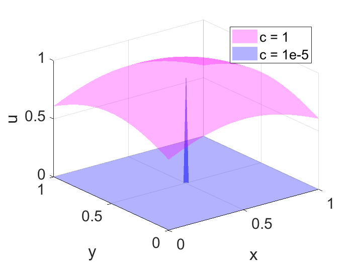
Figure 2: Shapes of the 2D solution on the unit square.

2.2 FEM formulation

For the weak form of FEM, we refer to [1]. The function spaces are defined based on Lagrangian polynomials. The element degree is denoted by $p$.

We implement FEM in deal.ii@ [8], where the IEEE-754 double precision is adopted. It basically contains the following steps: generating the grid, setting up the problem, assembling the system of equations, solving, and computing the error.

For the details of generating the grid, see Section 2.2.1. In the assembling process, for computing the occurring integrals, sufficiently accurate Gaussian quadrature formulas are used. In the solving process, the UMFPACK solver [9], which implements the multi-frontal LU factorization approach, is used. Using this solver prevents iteration errors associated with iterative solvers. For the error estimation, we refer to Section 2.2.2.

The above steps involve the following parameters associated with a computational mesh: the refinement level, grid size, number of DoFs, and error, which are denoted by $R$, $h$, $N$, and $E$, respectively. $R=0$ for the initial mesh, and it increases by one with each refinement. Note that, $E$ can also be the truncation error $E_{\rm T}$ or the round-off error $E_{\rm R}$.

Moreover, the use of two types of refinement strategies ushers in two sets of parameters. To differentiate the parameters of the adaptive refinement and the regular refinement, the notations in Table 1 are introduced.

Table 1: Differentiation of the parameters of the REG strategy and the AMR strategy.

	REG	AMR
$R$	$R^{\rm reg}$	$R^{\rm amr}$
$h$	$h^{\rm reg}$	$h^{\rm amr}$
$N$	$N^{\rm reg}$	$N^{\rm amr}$
$E$	$E^{\rm reg}$	$E^{\rm amr}$

2.2.1 Grid generation

For the adaptive refinement, the error estimator is chosen to be the Kelly estimator [10], which is based on the gradient derived from the numerical solution. For the mesh where we will conduct the adaptive refinement, we assume that the distribution of the error estimator is nonuniform [5]. Note that the grid sizes of different cells are not the same since not all cells are refined with one refinement, and we use the minimum grid size to represent the overall grid size.

2.2.2 Error estimation

The numerical error depends on $h$ and $p$. We can estimate the error either when $u_{h}$ is known or not, which are called a priori error estimation and a posteriori error estimation, respectively.

Using the former, the exact value of the error is not given, but an upper bound in provided. It follows that [11, 12]

$$\|u-u_{h}\|_{L^{2}}\leq Ch^{p+1}\|u\|_{H^{p+1}},$$ (2)

where $C$ is a constant, and $u_{h}$ denotes the numerical solution.

Using the latter, the exact value of the error is computed, where the reference solution is the exact solution or that from other sources. With respect to the latter, which is the general case, various methods, such as recovery methods, residual methods, and duality methods, can be used. In this paper, we use the recovery method. Specifically, the Richardson extrapolation where the reference solution is the finer solution with grid size $h/2$ is considered [13].

3 The optimal mesh for achieving a tolerance

In Section 3.1, we illustrate the influence of pct on both the truncation error and the round-off error. In Section 3.2, we propose a new method to select pct. For different problems, the numerical results of the new method can be found in Section 3.3.

3.1 Error reduction using the AMR strategy

When using the AMR strategy, different values of pct mean different degrees of error reduction. Specifically, the resulting truncation error basically decreases with an increasing percentage; if the pct is large enough, $E^{\rm amr}$ becomes stable, see the black circles in Fig. 3. Obviously, the stabilized $E^{\rm amr}$ is equal to $E^{\rm reg}$. Here, we denote the stabilized $E^{\rm amr}$ by $E_{\rm ref}$, and the smallest pct that can achieve it by pct_opt.

The pct_opt strongly depends on the distribution of the estimator. If the distribution consists of very localized structures, it is very small, whereas for the distribution with a global structure, it is close to 100% [7].

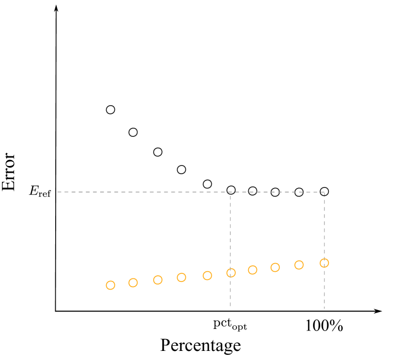
Figure 3: Influence of the pct on the error.

On the other hand, according to the results in Section 4, the round-off error increases with an increasing pct. The sketch of their relation are denoted by orange circles in Fig. 3.

3.2 A new method for seeking pct

For achieving a tolerance, to reduce the round-off error as much as possible, we propose to use pct_opt. As a first step, we obtain $E_{\rm ref}$ by conducting an extra regular refinement. Second, starting with one small pct, we test the pct in ascending order until pct_opt is found, where the increment of pct for each test is chosen to be 10% by experience.

For simplicity, the following abbreviations are introduced. We denote the present mesh by $M_{0}$; the pct used for each testing is denoted by pct_tst, and the resulting error by $E_{\rm tst}$. Specially, the initial pct_tst is denoted by pct_init, and the resulting error by $E_{\rm init}$. The selection of the pct_init, and the procedure for testing different pct_tst can be found below.

Step 1: selecting pct_init

It is slightly different for the first pct_opt and the remaining pct_opt. For the former, to capture the mesh locality as much as possible, pct_opt is chosen to be a relatively small number reading 5%. For the latter, we will choose the value based on the previous pct_opt, denoted by pct_prev. That is, pct_init is chosen to be slightly smaller than pct_prev since the distribution of the error estimator tends to become flatter with each adaptive refinement, where the formula used reads:

$$\text{pct}_{\rm init}=0.7\times\text{pct}_{\rm prev}.$$ (3)

Note that if the resulting pct_opt is larger than 85%, which indicates the distribution of the error estimator is smooth, we move to the REG strategy for the next refinement.

Step 2: seeking pct_opt

When a pct_init is obtained, we can start searching for pct_opt by setting pct_tst = pct_init.

First, we refine $M_{0}$ using pct_tst and compute $E_{\rm tst}$. Second, we compare $E_{\rm tst}$ with $E_{\rm ref}$: if $E_{\rm tst}\approx E_{\rm ref}$, we are satisfied with this pct_tst; otherwise, we increase the pct_tst. With this new pct_tst, if pct${}_{\rm tst}<95\%$, we repeat the above two stages; otherwise, we move to the regular refinement. The associated algorithm can be found in Algorithm 1, also in Fig. 4.

pct_tst $\leftarrow$ pct_init;

Refine $M_{0}$ and compute $E_{\rm tst}$;

while $E_{\rm tst}\not\approx E_{\rm ref}$ do

    pct_tst $\leftarrow$ pct_tst + 10%;

    if pct${}_{\rm tst}<95\%$ then

       Refine $M_{0}$ and compute $E_{\rm tst}$;

      

   else

       Move to the regular refinement;

      

    end if

   

end while

Algorithm 1 Seeking pct_opt

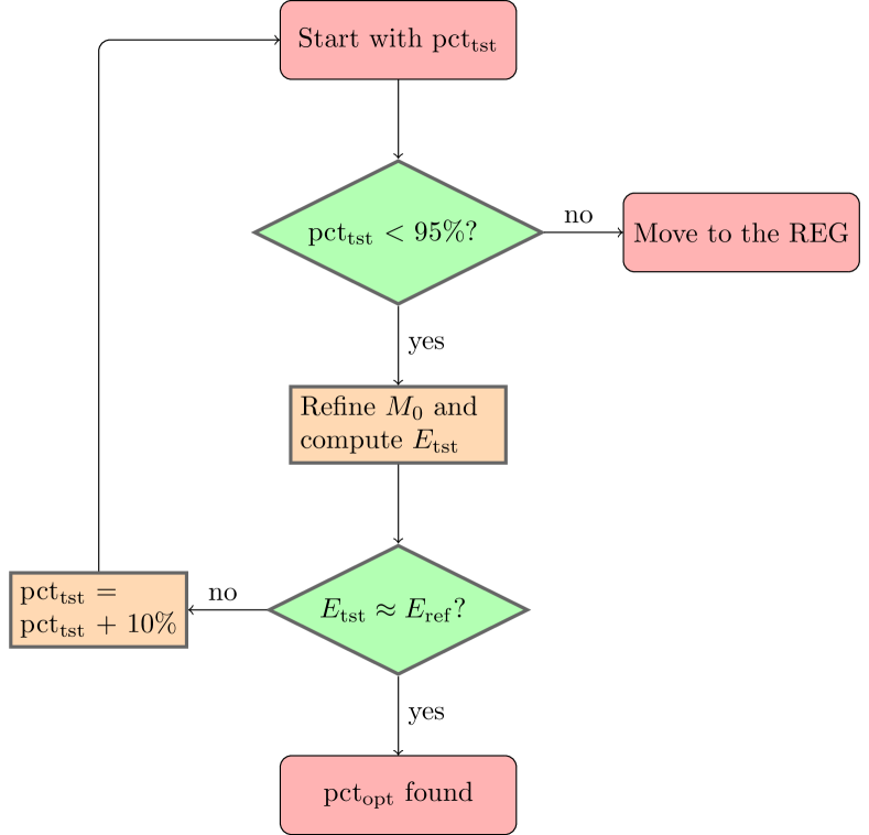
Figure 4: Illustration of the procedure for seeking pct_opt.

In summary, we obtain pct_opt by adding extra work. In what follows, we denote the $E_{\rm ref}$-oriented adaptive mesh refinement proposed above by EOAMR.

3.3 Results

We investigate the problem of Eq. (1) with $c$ = 1e-5. The initial mesh that suits for the load can be found in Fig. 5. As can be seen, since the load is very localized at the center, a smaller grid size is needed there. The element degree $p$ used reads 1 and 3. The results using the EOAMR can be found below.

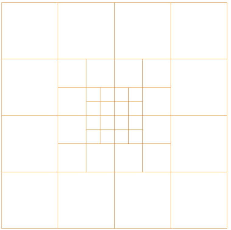
Figure 5: Initial mesh for the problem of Eq. (1) with $c=1e$-5.

For $p=1$, using the EOAMR, eight pct_opt are found. The first pct_opt is much smaller than 1, reading about 5%; from the second one to the sixth one, pct_opt does not change much, which remains smaller than 20%; from the seventh one, pct_opt quickly increases, see Fig. LABEL:comparison_of_EOAMR_to_REG_1p5_u_pct_deg_1 for the evolution of pct_opt.

For $p=3$, nine pct_opt are found. The evolution of pct_opt is similar with that for $p=1$, see Fig. LABEL:comparison_of_EOAMR_to_REG_1p5_u_pct_deg_3.

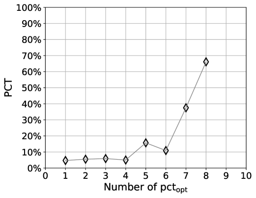
(a)

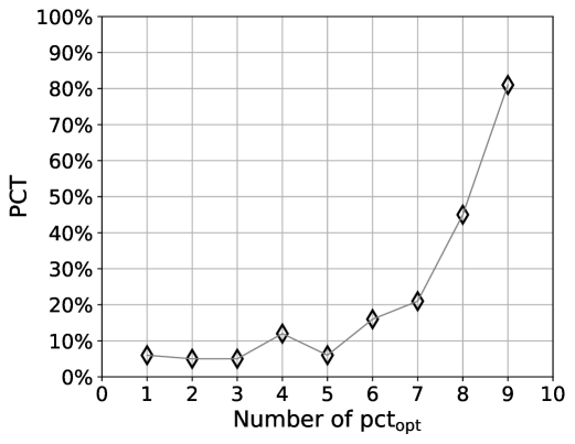
(b)

Figure 6: Evolution of pct_opt using EOAMR for the 2D Poisson problem of Eq. (1) with $c=$1e-5.

4 Round-off error in $h$-adaptive refinement

We use the method of manufactured solutions proposed in [1] to quantify the round-off error. We consider the 2D Poisson problem with $u=1$, and $p=2$ is investigated. Two scenarios are analyzed. One is using different pct on the same mesh to see its influence on the error. The other is using one constant pct to continually refine a mesh to study the error evolution. The details can be found below.

Using different pct on the same mesh

We consider different meshes in terms of the regular refinement level $R^{\rm reg}$, of which the value equals 2, 4, and 6, respectively. The pct ranges from 5% to 85%. For each mesh, the error evolution with the number of DoFs using different pct can be found in Fig. 7.

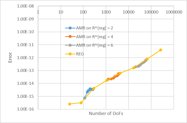
Figure 7: Errors using different pct on the same mesh.

As can be seen, for all the meshes, the error increases with the increasing pct. When the pct is close to 1, the error nearly reaches that using the regular refinement.

Using one constant pct to refine one mesh continually

Here, pct = 30% is chosen. The initial mesh is the regular mesh of $R^{\rm reg}=2$. The resulting errors can be found in Fig. 8.

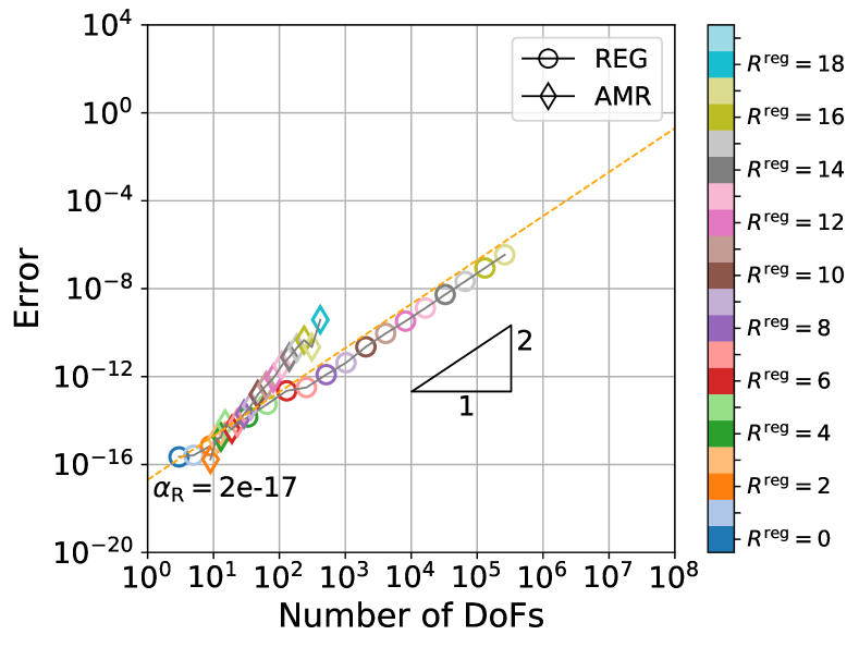
(a)

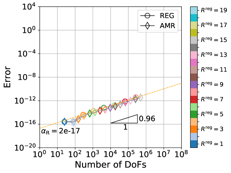
(b)

Figure 8: Comparison of the error evolution using the regular refinement and the adaptive refinement.

Fig. LABEL:error_evolution_h_reg_vs_h_amr_p_equal_to_2_h_as_x_axis indicates that by decreasing the grid size, $E_{\rm R}$ can either increase or decrease. For the latter, it can be verified by comparing the error of the fifth regular mesh to that of the seventh adaptive mesh, both counting from the right.

From Fig. LABEL:error_evolution_h_reg_vs_h_amr_p_equal_to_2_N_as_x_axis, $E_{\rm R}$ can be expressed by one function of $N$ when using the AMR strategy. Obviously, the expression of $E_{\rm R}$ as a function of $N$ is basically the same for both the REG strategy and the AMR strategy. However, this is not the case for 1D problems.

5 Conclusion

We propose a new marking strategy that selects elements for refinement so that AMR follows the same asymptotic error behavior as REG without the excessive amount of DOFs of the latter. When the solution is sharp, using the new strategy to seek a tolerance, the CPU time can be saved a lot compared with using the regular refinement. Our numerical experiments furthermore demonstrate that the round-off error does not depend on the minimum mesh width but on the total number of DoFs (i.e. it is a result of how many times we commit a round-off error). Hence, AMR not only reduces the amount of DOFs in regions where they are not needed to improve the accuracy but also mitigates the devastating effect of the round-off error and thereby enables more accurate solutions. This advantage of AMR becomes particularly pronounced for high-order approximations.

Appendix A A practical algorithm for finding $h_{\rm opt}$ when using the REG strategy

Normally, to reach one tolerance, we check if the tolerance is satisfied for each refinement level and stop further refinements when the tolerance is satisfied. Since $tol$ is reachable when $tol\geq E_{\rm min}$, one may waste a lot of CPU time if $tol$ cannot be reached.

To avoid unnecessary computations, we predict $N_{\rm opt}$ and the associated $E_{\rm min}$ in [1], of which the formula is derived from the perspective of the round-off error. Here, we will illustrate a slightly different version: to predict $h_{\rm opt}$ and the associated $E_{\rm min}$ from the perspective of satisfying the condition of the truncation error, which is more concise and easy to understand. For this strategy, the preliminaries and procedure can be found in A.1 and A.2, respectively. We show the application of the algorithm in Section A.3.

A.1 Preliminaries

We use the following properties of $E_{\rm T}$ and $E_{\rm R}$.

Truncation error

The a priori error estimation provides the theoretical convergence order of the error, which is for the validation purpose. Specifically, when $h$ is relatively small, the error converges to a formula [14, 11]:

$$E_{\rm T}=C_{\rm T}\cdot h^{q},$$ (4)

where $C_{\rm T}$ is a constant dependent on the element degree, and $q$ the analytical order of convergence, which equals $p+1$ when $p$ is smaller than ten approximately [15].

Round-off error

The round-off error is caused by the adoption of the finite precision arithmetic, of which the value is not reflected in Eq. (2). According to [16], it has a power-law relation with the number of DoFs. In the log-log plot where the $x$ axis is the number of DoFs, and the $y$ axis is the error, the round-off error increases along a straight line with the increasing number of DoFs. Denoting the slope and the offset of the line by $\alpha_{\rm R}$ and $\beta_{\rm R}$, respectively, the round-off error reads

$$E_{\rm R}=\alpha_{\rm R}\cdot{N}^{\beta_{\rm R}}.$$ (5)

In [16], we show that $\beta_{\rm R}$ is independent of different $f$, and $\alpha_{\rm R}$ is linearly proportional to $\|u\|_{2}$. For general problems, $\alpha_{\rm R}$ and $\beta_{\rm R}$ can be determined using the method of manufactured solutions [1].

Moreover, when $h$ is relatively small, $N$ is a function of $h$ and $p$ [1]:

$$N\approx\Bigl{(}\frac{p}{h}\Bigr{)}^{2},$$ (6)

which indicates that the number of DoFs basically quadruples with the increasing refinement level [1]. Therefore, substituting Eq. (6) into Eq. (5), we have the expression of $E_{\rm R}$ in terms of $h$:

$$E_{\rm R}=C_{\rm R}\cdot{h}^{D_{\rm R}},$$ (7)

where $C_{\rm R}=\alpha_{\rm R}\cdot p^{2\beta_{\rm R}}$, and $D_{\rm R}=-2\beta_{\rm R}$.

Now, from Eq. (4) and Eq. (7), when $q$ is satisfied, the total error in terms of $h$ reads

$$E=C_{\rm T}\cdot h^{q}+C_{\rm R}\cdot{h}^{D_{\rm R}}.$$ (8)

As can be seen, when $h$ is small, it basically follows that $E_{\rm T}>E_{\rm R}$; with the decreasing $h$, $E_{\rm T}$ decreases, and $E_{\rm R}$ increases.

Due to the interplay between $E_{\rm T}$ and $E_{\rm R}$, there is a minimum achievable error, which is denoted by $E_{\rm min}$, for which the corresponding $h$ is denoted by $h_{\rm opt}$.

A.2 Procedure for the prediction

From Eq. (8), we can predict the error when order $q$ is satisfied. First, we determine when $q$ is reached. Second, we derive the value of $C_{\rm T}$. Finally, we conduct the prediction.

Checking the condition of $q$

The practical value of $q$, denoted by $q_{h}$, is computed as follows.

$$q_{h}=\frac{\log\left(\frac{E_{h/2}}{E_{h}}\right)}{\log 2},$$ (9)

where $E_{h}$ and $E_{h/2}$ denote the errors with grid size $h$ and $h/2$, respectively.

When order $q$ is reached, error $E$, number of DoFs $N$, refinement level $R$ and grid size $h$ are denoted by $E_{\rm c}$, $N_{\rm c}$, $R_{\rm c}$ and $h_{\rm c}$, respectively. For different problems, $R_{\rm c}$ are different [17]. When the solution is smooth, $R_{\rm c}$ is relatively small. Note that in this paper, we assume $q$ is reachable if not stated otherwise, and the CPU time required is not very large.

Deriving the coefficient

The coefficient $C_{\rm T}$ is computed as follows.

$$C_{\rm T}=\frac{E_{\rm c}}{{h_{\rm c}}^{q}}.$$ (10)

Predicting the results

For the tolerance $tol$, the corresponding $N$, $h$, and $R$ are denoted by $N_{tol}$, $h_{tol}$, and $R_{tol}$, respectively. Specifically, when $tol=E_{\rm min}$, they are denoted by $N_{\rm opt}$, $h_{\rm opt}$, and $R_{\rm opt}$, respectively.

For Eq. (8), $$h_{\rm opt} E_{\rm min}$$ and are predicted as follows:

$$h_{\rm opt}^{\rm PRED} =\left(-\frac{C_{\rm T}\cdot q}{C_{\rm R}\cdot D_{\rm R}}\right)^{\frac{1}{D_{\rm R}-q}},$$ (11a)

$$E_{\rm min}^{\rm PRED} =C_{\rm T}\cdot{h_{\rm opt}}^{q}+C_{\rm R}\cdot{h_{\rm opt}}^{D_{\rm R}},$$ (11b)

where $$E_{\rm min}^{\rm PRED} N_{tol}^{\rm PRED} E_{\rm min} N_{\rm opt} E_{\rm min} N_{\rm opt} E_{\rm min}^{\rm BF} N_{tol}^{\rm BF}$$ and denote the predicted and , respectively. Moreover, using the BF approach, and are denoted by and , respectively.

A.3 Application

Using the PRED method, we can relatively quickly determine if an accuracy can be reached. For a given $tol$, one $p$ is possible when $tol\geq E_{\rm min}^{\rm PRED}$. With respect to $h_{tol}$, it is predicted by

$$h_{tol}^{\rm PRED}={\Big{(}\frac{tol}{C_{\rm T}}\Big{)}}^{\frac{1}{q}},$$ (12)

where $h_{tol}^{\rm PRED}$ denotes the predicted $h_{tol}$. With $h_{tol}^{\rm PRED}$, we can directly compute the solution of interest, and hence several refinement steps before $h_{tol}^{\rm PRED}$ can be reduced compared to REG. When $tol$ cannot be reached, we stop further refinements.

The reduction of the refinement steps indicates the reduction of the CPU time. Specifically, when $tol$ can be reached, the CPU time reduction is not much compared with the BF method because we still have to compute the solution for $h_{tol}^{\rm PRED}$, and the CPU time reduced is not as much as that for computing the solution for $h_{tol}^{\rm PRED}$; otherwise, the reduction of the CPU time is much more.

References

- [1] Jie Liu, Henk M Schuttelaars, and Matthias Möller. A practical algorithm to minimize the overall error in fem computations. arXiv preprint arXiv:2202.02572, 2022.
- [2] Joel H Ferziger and Milovan Peric. Computational methods for fluid dynamics. Springer Science & Business Media, 2012.
- [3] Marsha J Berger and Joseph Oliger. Adaptive mesh refinement for hyperbolic partial differential equations. Journal of computational Physics, 53(3):484–512, 1984.
- [4] Julen Alvarez-Aramberri, David Pardo, Maciej Paszynski, Nathan Collier, Lisandro Dalcin, and Victor M Calo. On round-off error for adaptive finite element methods. Procedia Computer Science, 9:1474–1483, 2012.
- [5] Willy Dörfler. A convergent adaptive algorithm for poisson’s equation. SIAM Journal on Numerical Analysis, 33(3):1106–1124, 1996.
- [6] John Francis Dannenhoffer. Grid adaptation for complex two-dimensional transonic flows. PhD thesis, Massachusetts Institute of Technology, 1987.
- [7] Kévin Pons and Mehmet Ersoy. Adaptive mesh refinement method. part 1: Automatic thresholding based on a distribution function. HAL open science, 2019.
- [8] Daniel Arndt, Wolfgang Bangerth, Bruno Blais, Marc Fehling, Rene Gassmöller, Timo Heister, Luca Heltai, Uwe Köcher, Martin Kronbichler, Matthias Maier, Peter Munch, Jean-Paul Pelteret, Sebastian Proell, Konrad Simon, Bruno Turcksin, David Wells, and Jiaqi Zhang. The deal.ii library, version 9.3. Journal of Numerical Mathematics, 29(3):171–186, 2021.
- [9] Timothy A Davis. Algorithm 832: UMFPACK V4.3 – an unsymmetric-pattern multifrontal method. ACM Transactions on Mathematical Software (TOMS), 30(2):196–199, 2004.
- [10] Donald W Kelly, JP De SR Gago, Olgierd C Zienkiewicz, and I Babuska. A posteriori error analysis and adaptive processes in the finite element method: Part i—error analysis. International journal for numerical methods in engineering, 19(11):1593–1619, 1983.
- [11] Mark S Gockenbach. Understanding and implementing the finite element method, volume 97. Siam, 2006.
- [12] Zhangxin Chen. Finite element methods and their applications. Springer Science & Business Media, 2005.
- [13] Ludovic Chamoin and Frederic Legoll. A pedagogical review on a posteriori error estimation in finite element computations. arXiv preprint arXiv:2110.02160, 2021.
- [14] Convergence of fem. [Online; accessed 22-June-2022].
- [15] William F Mitchell. How high a degree is high enough for high order finite elements? Procedia Computer Science, 51:246–255, 2015.
- [16] Jie Liu, Matthias Möller, and Henk M Schuttelaars. Balancing truncation and round-off errors in FEM: One-dimensional analysis. Journal of Computational and Applied Mathematics, 386:113219, 2021.
- [17] Olof Runborg. Verifying Numerical Convergence Rates. KTH Computer Science and Communication, 2012.