Strategic Prompt Pricing for AIGC Services: A User-Centric Approach

Abstract

The rapid growth of AI-generated content (AIGC) services has created an urgent need for effective prompt pricing strategies, yet current approaches overlook users’ strategic two-step decision-making process in selecting and utilizing generative AI models. This oversight creates two key technical challenges: quantifying the relationship between user prompt capabilities and generation outcomes, and optimizing platform payoff while accounting for heterogeneous user behaviors. We address these challenges by introducing prompt ambiguity, a theoretical framework that captures users’ varying abilities in prompt engineering, and developing an Optimal Prompt Pricing (OPP) algorithm. Our analysis reveals a counterintuitive insight: users with higher prompt ambiguity (i.e., lower capability) exhibit non-monotonic prompt usage patterns, first increasing then decreasing with ambiguity levels, reflecting complex changes in marginal utility. Experimental evaluation using a character-level GPT-like model demonstrates that our OPP algorithm achieves up to $31.72\%$ improvement in platform payoff compared to existing pricing mechanisms, validating the importance of user-centric prompt pricing in AIGC services.

I Introduction

With impressive progress in generative artificial intelligence (GAI) [1], AI-generated content (AIGC) services are growing in popularity, evidenced by platforms such as Monica [2] and Poe [3]. Figure 1 illustrates a typical framework of the AIGC service process, where the platform usually integrates multiple GAI models, e.g., GPT-4 [4] and GPT-4o [5], each with different performance of generating content in response to user prompts. Users will purchase AIGC services from the platform under a usage metric, i.e., the number of prompts [6], to interact with distinct models and obtain desired content.

This novel AI service paradigm has promoted the emergence of related research [7, 8, 9, 10, 11, 12], as summarized in surveys [13, 14, 15]. For example, Du et al. in [7] designed a dynamic service selection scheme to enhance AIGC quality. Dütting et al. in [8] proposed an AIGC advertising auction mechanism.

Figure 1: Framework of AIGC Service Process.

Liu et al. in [12] incorporated semantic communication to achieve efficient content generation. However, these studies primarily address AIGC service optimization, leaving a significant research gap in platform prompt pricing design.

Current prompt pricing (e.g., [2, 3, 16]) typically relies on GAI models’ cost or performance metric, neglecting users’ strategic decision-making process. In AIGC services, the platform decides the prompt price of each model and necessitates users to make two-step utilization decisions: which model to utilize and how to utilize it (i.e., the number of prompts for interaction [6, 15]). Users will decide both the optimal model and prompt number to maximize individual payoff, based on their varying prompt capabilities [17]. Failing to account for such heterogeneous decisions in prompt pricing could not only reduce the platform’s payoff, but also discourage users (e.g., those with low prompt capability) from AIGC services. Thus, to design the optimal prompt pricing mechanism, we first delve into users’ strategic decisions in AIGC services, which motivates our key question as follows:

Key Question 1.

What is the optimal utilization strategy for users with different prompt capabilities in AIGC services?

The prompt-based content generation of AIGC services poses unique challenges to user decision-making. Specifically, the user’s utility derived from generated content depends on both model performance and user prompts (i.e., prompt number and quality, as highlighted in [17, 18]). This correlation and inherent uncertainty [19] make it difficult to assess each prompt’s value across diverse models and users, complicating decisions on selecting and prompting GAI models.

To address the above challenges from interactions between models and prompts, we introduce the concept of prompt ambiguity, inspired by in-context learning [20, 21, 22]. This mathematical framework quantifies user prompts as the probability of correctly conveying the intended task, enabling us to derive optimal utilization decisions for heterogeneous users. With users’ optimal strategy in AIGC services, we can study our second key question of this paper:

Key Question 2.

What is the platform’s optimal prompt pricing mechanism for AIGC services?

The design of optimal prompt pricing presents a challenging bi-level non-convex optimization problem, due to the heterogeneity of users’ prompt capabilities and strategic decisions. The platform must maximize payoff while accounting for users’ two-step decision-making process, forming a complex bi-level structure. Prompt prices across various GAI models are also ineluctably intertwined with the trade-off between user strategies in selecting and prompting the model, resulting in the non-convexity of this mechanism design problem.

Against this background, we first transform the problem into an unconstrained piecewise form to determine optimal prompt pricing for users with consistent prompt capabilities (homogeneous case). Then, by exploring the relationship between user utilization decisions and model prompt prices in this simplified scenario, we establish the price upper bound for the more general heterogeneous user case. According to these insights, we propose an Optimal Prompt Pricing (OPP) algorithm, which decomposes prompt pricing design into tractable sub-problems for platform payoff maximization.

The key results and contributions of the paper are as follows:

• Optimal Prompt Pricing Framework: We address the fundamental challenge of modeling strategic interactions between the platform and heterogeneous users in AIGC services. Our framework transforms this bi-level optimization problem into tractable sub-problems through theoretical bounds analysis, providing the first systematic solution for prompt-based pricing mechanisms.

• User Utilization Strategy Analysis: We tackle the challenge of quantifying diverse user prompt capabilities in AIGC services. By introducing prompt ambiguity based on in-context learning [20, 21, 22], we establish a mathematical framework that precisely captures how users select and interact with different GAI models.

• Impact of User Prompt Ambiguity: We solve the non-intuitive relationship between user prompt capability and optimal prompt usage. Our analysis reveals that higher prompt ambiguity (lower capability) creates a non-monotonic pattern in prompt number: first increases and then decreases with ambiguity levels, corresponding to variations in user marginal utility of additional prompts.

• Experimental Evaluation: We bridge the gap between theoretical analysis and practical implementation using a character-level GPT-like model [23] and synthetic language data set [20, 21, 22]. The extensive experiments validate our analysis and demonstrate that our proposed OPP algorithm can improve the platform’s payoff by up to $31.72\%$, compared to existing pricing mechanisms.

The remainder of this paper is organized as follows. Section II presents the system model and problem formulation in AIGC services. Section III and Section IV respectively derive heterogeneous users’ optimal utilization strategies and the platform’s optimal prompt pricing. We provide experimental evaluation in Section V and conclude the paper in Section VI. Due to the page limit, we leave detailed proofs of our results and additional theoretical analysis in the online appendix [24].

II System Model and Problem Formulation

In this section, we first introduce the AIGC service process, a two-stage Stackelberg game between users and the platform. Then, we elaborated on modeling heterogeneous users and the platform’s optimal prompt pricing mechanism design problem.

II-A The AIGC Service Process

We consider a typical two-stage process of AIGC services between heterogeneous users and a platform, outlined below:

• Stage 1: Platform publishes a set of GAI models, each with a specific prompt price and performance characteristic of generating content in response to user prompts.

• Stage 2: Users make two-step utilization decisions for AIGC services, determining which GAI model to utilize and the number of prompts required for its utilization.

Figure 2: Two-stage Stackelberg Game of AIGC Services.

Next, we present each stage in detail, depicted in Figure 2.

II-A1 Stage 1

The platform offers a set of GAI models with different performances and decides each model’s prompt price.

• Published GAI Model Set: The platform publishes a set of GAI models $\mathcal{M}=\{M_{L},M_{H}\}$ with distinct performance tiers: a low-performance model $M_{L}$ and a high-performance model $M_{H}$. This binary categorization, prevalent in existing platforms (e.g., [2, 3, 16]), enables focused theoretical analysis while maintaining generalizability to multi-model scenarios.

• Prompt Prices: The platform establishes prompt prices $\boldsymbol{p}=\{p_{m},\forall m\in\mathcal{M}\}$, where $p_{m}$ denotes the price per prompt for model $m\in\mathcal{M}$. This usage-based pricing scheme aligns with current industry practices. For example, Poe [3] charges approximately $\$0.008$ per prompt for GPT-4 [4] and $\$0.01$ for GPT-4o [5].

• Operational Costs: Each prompt incurs operational costs for the platform, represented by $\mathcal{C}=\{C_{m},\forall m\in\mathcal{M}\}$, where $C_{m}$ denotes the per-prompt cost for GAI model $m\in\mathcal{M}$. These costs encompass both computation [6] and communication [15] resources. For reference, GPT-4’s operational cost is about $\$0.0036$ per prompt [25].

II-A2 Stage 2

Users decide both which GAI model to utilize and the number of prompts required for its utilization.

• Model Selection: Users choose a specific model $s\in\mathcal{M}$ from the available options based on the platform’s published model set $\mathcal{M}$ and pricing strategy $\boldsymbol{p}$.

• Prompt Strategy: Users determine the optimal number of prompts $n\in\mathbb{N}$ needed for their task. This decision depends on both the selected model’s performance and the user’s prompt capability.

These decisions in Stage 2 are interdependent, and their optimal values are analyzed in detail in the following section.

II-B Modeling of Heterogeneous Users

This subsection characterizes the user’s prompt behaviors, expected utility, and expected payoff in AIGC services.

II-B1 User’s Prompt Behaviors

Users interact with GAI models by conveying a specific intention (task) through prompts to generate desired content, such as instructions like “avoid long sentences” or “highlight key messages” when polishing text (see Figure 3). To formalize this interaction, we establish a mathematical framework where $\Gamma$ denotes a discrete and complete space of user intentions, with each intention $\gamma\in\Gamma$ being unique, and $\mathcal{X}_{\gamma}$ represents the set of user prompts associated with intention $\gamma$. Each prompt $x\in\mathcal{X}_{\gamma}$ is independently generated from a distribution [26, 27] conditioned on the corresponding intention $\gamma$, providing a foundational structure for analyzing user-model interactions in AIGC services.

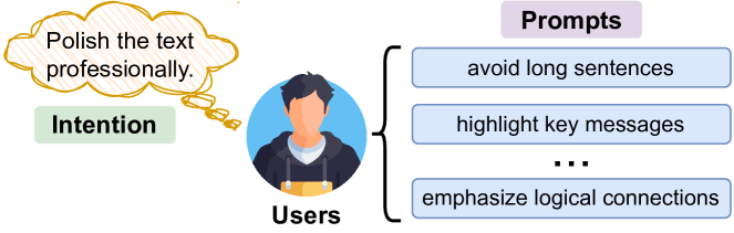
Figure 3: Example of User Prompts and Intention.

In practice, users’ varying prompt capabilities often result in ambiguous communication of their target intention $\gamma\in\Gamma$. Drawing from in-context learning literature [20, 21, 22], we introduce the concept of prompt ambiguity to quantify these heterogeneous prompt capabilities:

Definition 1 (Prompt Ambiguity).

A user prompt $x\in\mathcal{X}_{\gamma}$ is $\epsilon$-ambiguous for intention $\gamma\in\Gamma$ with $\epsilon\in(0,1)$, if

$$\textrm{Prob}\left(\gamma|x\right)\geq 1-\epsilon,$$ (1)

which indicates that the probability of correctly inferring the target intention $\gamma$ from user prompt $x$ is at least $1-\epsilon$.

Building upon Definition 1 and existing literature [20, 21, 22], we establish the relationship between user prompts and target intention in Lemma 1.

Lemma 1.

For a user with prompt ambiguity $\epsilon$, the probability of inferring target intention $\gamma\in\Gamma$ from $k\in\mathbb{N}^{+}$ prompts is:

$$\text{Prob}(\gamma_{1}=\gamma,\cdots,\gamma_{k}=\gamma|x_{1},\cdots,x_{k})\geq 1-\epsilon^{k},$$ (2)

where $x_{k}$ denotes the user’s $k$-th prompt and $\gamma_{k}$ represents the intention conveyed by prompt $x_{k}$, for any $k\in\mathbb{N}^{+}$.

The detailed proof of Lemma 1 is provided in the appendix [24]. To capture the diversity in users’ prompt capabilities, we employ a probability density function $f(\epsilon)$ to characterize the distribution of prompt ambiguity across the user population.

II-B2 User’s Expected Utility

Within intention space $\Gamma$, a user’s utility from generated content is determined by two factors: the selected model’s performance and the probability of successfully conveying the target intention through prompts. For any published model $m\in\mathcal{M}$, we define $U_{m}$ as the utility that maps from intention space to generated content, indicating the model’s performance in responding to user intentions (e.g., prediction accuracy in semantic tasks [20]). Accordingly, the utility mapping of the user’s selected model $s\in\mathcal{M}$ is $U_{s}$. Based on Lemma 1, for a user’s GAI model selection $s\in\mathcal{M}$, prompt number $n\in\mathbb{N}$, and prompt ambiguity $\epsilon\in(0,1)$, the user’s expected utility is expressed as:

$$\left(1-\epsilon^{n}\right)\cdot U_{s},$$ (3)

where $U_{s}$ represents the utility of model $s\in\mathcal{M}$.

II-B3 User’s Expected Payoff

The user’s payoff $\pi_{\text{user}}$ is defined as the difference between expected utility $(1-\epsilon^{n})U_{s}$ and the total prompting price $np_{s}$:

$$\pi_{\textrm{user}}(s,n,\boldsymbol{p},\epsilon)=\left(1-\epsilon^{n}\right)\cdot U_{s}-n\cdot p_{s}.$$ (4)

Users make optimal decisions by selecting model choice $s^{*}\in\mathcal{M}$ and prompt number $n^{*}\in\mathbb{N}$ to maximize payoff $\pi_{\text{user}}$ in (4). These decisions are based on prompt prices $\boldsymbol{p}$ and their individual prompt ambiguity $\epsilon\in(0,1)$. To emphasize the interdependence between optimal decisions, we denote them as $s^{*}(n^{*},\boldsymbol{p})$ and $n^{*}(s,p_{s},\epsilon)$, respectively. This formalization provides the foundation for analyzing the platform’s prompt pricing mechanism design problem.

II-C Platform’s Prompt Pricing Mechanism Design Problem

In AIGC services, the platform decides the optimal prompt pricing $\boldsymbol{p}^{*}=\{p_{m}^{*},\forall m\in\mathcal{M}\}$ to maximize its payoff across all GAI models and users. We first summarize the platform’s expected payoff $\pi_{\textrm{platform}}(\boldsymbol{p})$ and then formally introduce its problem of prompt pricing mechanism design.

For the platform, its expected payoff $\pi_{\textrm{platform}}(\boldsymbol{p})$ is the aggregate of that from each GAI model. Specifically, given any model $m\in\mathcal{M}$, the platform’s per-prompt payoff is $p_{m}-C_{m}$, where $p_{m}$ and $C_{m}$, respectively, represent the model’s prompt price and prompt cost. Through the prompt ambiguity density function $f(\epsilon)$, we can further determine the expected number of user prompts for model $m\in\mathcal{M}$:

$$N_{m}(\boldsymbol{p})=\int_{0}^{1}f(\epsilon)\cdot n^{*}(m,p_{m},\epsilon)\cdot\mathds{1}_{s^{*}(n^{*},\boldsymbol{p})=m}\,d\epsilon,$$ (5)

where indicator function $\mathds{1}_{s^{*}(n^{*},\boldsymbol{p})=m}$ indicates that the optimal GAI model for the user is $m\in\mathcal{M}$. Accordingly, the expected payoff of the platform in AIGC services is:

$$\pi_{\textrm{platform}}(\boldsymbol{p})= \sum\nolimits_{m\in\mathcal{M}}\left(p_{m}-C_{m}\right)\cdot N_{m}(\boldsymbol{p}).$$ (6)

To maximize payoff $\pi_{\textrm{platform}}(\boldsymbol{p})$ in (6), the platform needs to account for each user’s self-interested decisions $s^{*}(n^{*},\boldsymbol{p})$ and $n^{*}(s,p_{s},\epsilon)$. By incorporating heterogeneous users’ strategic decisions, we formulate the platform’s optimal prompt pricing problem as a bi-level optimization in Problem 1.

Having established the system model and problem formulation for AIGC services, we tackle this two-stage Stackelberg game using backward induction [28]. Our study follows a sequential approach: Section III examines users’ strategic utilization decisions in Stage 2, and subsequently, Section IV leverages these insights to derive the platform’s optimal prompt pricing mechanism in Stage 1.

III Heterogeneous Users’ Utilization Strategy

This section analyzes heterogeneous users’ optimal utilization strategies in AIGC services. Our analysis progresses from single-user optimization to multiple-user scenarios, revealing how prompt ambiguity and pricing affect users’ strategic behaviors and expected payoff.

III-A The User’s Optimal Utilization Strategy

According to the published model set $\mathcal{M}$ and prompt pricing $\boldsymbol{p}=\{p_{m},\forall m\in\mathcal{M}\}$, each user maximizes individual payoff $\pi_{\textrm{user}}(s,n,\boldsymbol{p},\epsilon)$ by deciding the optimal model $s^{*}(n^{*},\boldsymbol{p})$ and prompt number $n^{*}(s,p_{s},\epsilon)$. Given model decision $s\in\mathcal{M}$ and ambiguity $\epsilon\in(0,1)$, Theorem 1 derives the optimal prompt strategy $n^{*}(s,p_{s},\epsilon)$ for the user.

Theorem 1.

For any selected model $s\in\mathcal{M}$ with utility mapping $U_{s}$ and prompt price $p_{s}$, a user with prompt ambiguity $\epsilon\in(0,1)$ has the following optimal strategy:

$$n^{*}(s,p_{s},\epsilon)= \hskip-3.0pt\lfloor\log_{\epsilon}\frac{\epsilon p_{s}}{(1-\epsilon)U_{s}}\rfloor,\hskip-9.0pt 0\leq p_{s}\leq(1-\epsilon)U_{s},$$ if (7a)

$$n^{*}(s,p_{s},\epsilon)= \hskip-3.0pt0, p_{s}>(1-\epsilon)U_{s}$$ if , (7b)

where $\lfloor\cdot\rfloor$ is the floor function.

We give the proof of Theorem 1 in online appendix [24]. Theorem 1 provides a theoretical foundation for understanding the relationship between optimal prompt number $n^{*}(s,p_{s},\epsilon)$ and two key factors: prompt price $p_{s}$ and utility mapping $U_{s}$. For any selected model $s\in\mathcal{M}$, utility mapping $U_{s}$ establishes a price ceiling of $(1-\epsilon)U_{s}$ that a user with ambiguity $\epsilon$ will accept. The optimal number of prompts will increase with $U_{s}$ and decrease with prompt price $p_{s}$.

Following Theorem 1, we can conclude the user’s optimal model selection $s^{*}(n^{*},\boldsymbol{p})$ from model set $\mathcal{M}$:

$$s^{*}(n^{*},\boldsymbol{p})=\operatorname*{argmax}\nolimits_{s\in\mathcal{M}} (1-\epsilon\char 94\relax{\lfloor\log_{\epsilon}\frac{\epsilon p_{s}}{(1-\epsilon)U_{s}}\rfloor})\cdot U_{s}$$

$$-\lfloor\log_{\epsilon}\frac{\epsilon p_{s}}{(1-\epsilon)U_{s}}\rfloor\cdot p_{s}.$$ (8)

This formulation captures the balance between utility maximization and price minimization in model selection.

III-B Multiple Users with Heterogeneous Prompt Ambiguities

After studying single user’s utilization decisions $s^{*}(n^{*},\boldsymbol{p})$ and $n^{*}(s,p_{s},\epsilon)$, we proceed to extend our analysis to encompass multiple users with heterogeneous prompt ambiguities. In particular, we start from the upper bound of heterogeneous users’ optimal prompt number $\bar{n}^{*}(m)\in\mathbb{N}^{+}$ in Lemma 2, in order to investigate the impact of ambiguity $\epsilon$ on users’ optimal strategies. This will form the foundation for designing the optimal prompt pricing mechanism in Stage 1.

Lemma 2.

For users with varying ambiguity $\epsilon\in(0,1)$, the upper bound $\bar{n}^{*}(m)$ on users’ optimal prompt number to GAI model $m\in\mathcal{M}$ is:

$$\bar{n}^{*}(m)=\min\left\{k\in\mathbb{N}^{+}:\frac{k^{k}}{(k+1)^{k+1}}<\frac{p_{m}}{U_{m}}\right\}.$$ (9)

Lemma 2 identifies the critical ratio ${p_{m}}/{U_{m}}$ that affects the upper bound $\bar{n}^{*}(m)$ of heterogeneous users’ optimal prompt number for model $m\in\mathcal{M}$. Building on this, Proposition 1 elaborates on the relationship between prompt ambiguity $\epsilon\in(0,1)$ and the optimal prompt strategy $n^{*}(s,p_{s},\epsilon)$ of users.

Proposition 1.

Given model decision $s\in\mathcal{M}$, utility mapping $U_{s}$ and prompt price $p_{s}$, users’ optimal prompt strategy $n^{*}(s,p_{s},\epsilon)$ varies with ambiguity $\epsilon\in(0,1)$ as follows:

• if $p_{s}=0$: $n^{*}(s,p_{s},\epsilon)=\infty$.

• if $p_{s}\in(0,U_{s}/4]$: $n^{*}(s,p_{s},\epsilon)$ first increases and then decreases with $\epsilon$.

• if $p_{s}\in(U_{s}/4,U_{s})$: $n^{*}(s,p_{s},\epsilon)$ decreases with $\epsilon$.

• if $p_{s}\in[U_{s},\infty)$: $n^{*}(s,p_{s},\epsilon)=0$.

We give the proof of Proposition 1 in appendix [24]. Proposition 1 reveals that users’ optimal prompt strategy exhibits non-monotonic variation with ambiguity $\epsilon$. The behavior can be categorized into three distinct cases, depicted in Figure 4:

• Extreme Cases: When $p_{s}=0$ or $p_{s}\geq U_{s}$, users either continuously prompt the model $s\in\mathcal{M}$ or completely avoid AIGC services of model $s\in\mathcal{M}$.

  

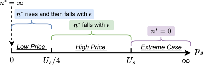
  Figure 4: The Optimal Prompt Number $n^{*}(s,p_{s},\epsilon)$ of Users with Varying Levels of Prompt Ambiguity $\epsilon\in(0,1)$.

• Low Price Range ($p_{s}\in(0,U_{s}/4]$): The optimal prompt number follows an inverse U-shaped pattern as ambiguity rises. Users with moderate prompt capability will use more prompts than those with very high or low capabilities, due to higher marginal utility of additional prompts.

• High Price Range ($p_{s}\in(U_{s}/4,U_{s})$): Decreased prompt capability (higher ambiguity $\epsilon$) consistently reduces the optimal prompt number. The elevated price amplifies the disadvantage of lower prompt capability, discouraging users with higher prompt ambiguity from AIGC services.

III-C The User’s Optimal Expected Payoff

Given the prompt strategy $n^{*}(s,p_{s},\epsilon)\in\mathbb{N}$ in Theorem 1 and GAI model decision $s^{*}(n^{*},\boldsymbol{p})\in\mathcal{M}$ in (III-A), we summarize the user’s optimal payoff $\pi_{\textrm{user}}^{*}(s^{*},n^{*},\boldsymbol{p},\epsilon)$ as follows:

$$\pi_{\textrm{user}}^{*}(s^{*},n^{*},\boldsymbol{p},\epsilon)= \left(1-\epsilon^{n^{*}(s^{*},p_{s^{*}},\epsilon)}\right)\cdot U_{s^{*}}$$

$$-n^{*}(s^{*},p_{s^{*}},\epsilon)\cdot p_{s^{*}},$$ (10)

where $U_{s^{*}}$ and $p_{s^{*}}$ are the utility mapping and prompt price of the user’s optimal model $s^{*}(n^{*},\boldsymbol{p})\in\mathcal{M}$, respectively.

With $\pi_{\textrm{user}}^{*}(s^{*},n^{*},\boldsymbol{p},\epsilon)$ in (III-C), we aim to discuss the effect of prompt ambiguity $\epsilon\in(0,1)$ on the user’s optimal expected payoff, as concluded in Proposition 2.

Proposition 2.

The user’s optimal payoff $\pi_{\textrm{user}}^{*}(s^{*},n^{*},\boldsymbol{p},\epsilon)$ decreases with prompt ambiguity $\epsilon\in(0,1)$.

Given the complex nature of users’ two-step decisions (as illustrated in Proposition 1), the proof of Proposition 2 requires careful analysis and is provided in detail in appendix [24]. This proposition indicates a crucial insight: while users may adapt their prompt strategy $n^{*}(s,p_{s},\epsilon)$ in various ways depending on the ratio $p_{s}/U_{s}$ (particularly when $p_{s}/U_{s}\in(0,1/4]$), their optimal payoff $\pi_{\textrm{user}}^{*}(s^{*},n^{*},\boldsymbol{p},\epsilon)$ invariably decreases as ambiguity $\epsilon$ increases. This demonstrates that despite users’ strategic adjustments to maximize their payoff under different ambiguity levels, the negative impact of increased prompt ambiguity on the optimal payoff cannot be fully mitigated.

Having completed our analysis of heterogeneous users’ optimal decisions and payoffs, we now proceed to examine the optimal prompt pricing in Stage 1 of AIGC services.

IV Platform’s Prompt Pricing Mechanism Design

This section derives the platform’s optimal prompt pricing mechanism by examining two distinct user scenarios. First, we focus on users with consistent prompt ambiguity, i.e., homogeneous cases, to establish a closed-form solution for optimal pricing. Then, based on these theoretical results, we extend our analysis to heterogeneous users and develop an efficient prompt pricing algorithm for platform payoff maximization.

IV-A The Optimal Prompt Pricing for Homogeneous Users

For a published GAI model set $\mathcal{M}$, the platform aims to determine the optimal prompt pricing $\boldsymbol{p}^{*}=\{p_{m}^{*},\forall m\in\mathcal{M}\}$ that maximizes its payoff $\pi_{\textrm{platform}}(\boldsymbol{p})$ in (6), formulated as a bi-level optimization in Problem 1. Theorem 2 establishes the optimal prompt price for each model when serving homogeneous users with prompt ambiguity $\epsilon\in(0,1)$.

Theorem 2.

For a model set $\mathcal{M}$ where each model $m\in\mathcal{M}$ has utility mapping $U_{m}$ and prompt cost $C_{m}$, the platform’s optimal prompt pricing $\boldsymbol{p}^{*}=\{p_{m}^{*},\forall m\in\mathcal{M}\}$ for homogeneous users with prompt ambiguity $\epsilon\in(0,1)$ is:

$$p_{m}^{*}= \epsilon^{\sigma(m,\epsilon)-1}(1-\epsilon)U_{m}, m=m^{*}$$ if , (11a)

$$p_{m}^{*}= U_{m}, m\neq m^{*}$$ if , (11b)

where $\sigma(m,\epsilon)=\min\{k\in\mathbb{N}:(k+1)\epsilon^{k}-k\epsilon^{k-1}<\frac{C_{m}}{(1-\epsilon)U_{m}}\}$ and $m^{*}=\operatorname*{argmax}_{m\in\mathcal{M}}(\epsilon^{\sigma(m,\epsilon)-1}(1-\epsilon)U_{m}-C_{m})\cdot\sigma(m,\epsilon)$.

We give the proof of Theorem 2 in the online appendix [24]. Theorem 2 formalizes the optimal prompt price $p_{m}^{*}$ of each model $m\in\mathcal{M}$, which increases with utility mapping $U_{m}$ and decreases with prompt cost $C_{m}$.

Building on Theorem 2, and in preparation for designing prompt pricing with heterogeneous users, we further need to understand the impact of ambiguity $\epsilon$ on optimal pricing $\boldsymbol{p}^{*}$.

Corollary 1.

For model $m^{*}\in\mathcal{M}$ with utility mapping $U_{m^{*}}$, prompt cost $C_{m^{*}}$, and optimal prompt price $p^{*}_{m^{*}}$, the user’s optimal strategy $n^{*}(m^{*},p^{*}_{m^{*}},\epsilon)$ varies with prompt ambiguity $\epsilon\in(0,1)$ as follows:

• if $C_{m^{*}}=0$: $n^{*}(m^{*},p^{*}_{m^{*}},\epsilon)$ increases with $\epsilon$.

• if $C_{m^{*}}\in(0,U_{m^{*}}/8]$: $n^{*}(m^{*},p^{*}_{m^{*}},\epsilon)$ first increases and then decreases with $\epsilon$.

• if $C_{m^{*}}\in(U_{m^{*}}/8,U_{m^{*}})$: $n^{*}(m^{*},p^{*}_{m^{*}},\epsilon)$ decreases with $\epsilon$.

• if $C_{m^{*}}\in[U_{m^{*}},\infty)$: $n^{*}(m^{*},p^{*}_{m^{*}},\epsilon)=0$.

We give the proof of Corollary 1 in appendix [24]. This relationship between prompt cost and optimal strategy is illustrated in Figure 5. In zero-cost scenario ($C_{m^{*}}=0$), increasing ambiguity leads the platform to encourage more prompts to maximize payoff. For low cost ($C_{m^{*}}\in(0,U_{m^{*}}/8]$), the platform initially reduces prices as ambiguity grows to stimulate higher prompt numbers, but beyond a threshold, it raises prices, reducing prompt usage. With higher cost ($C_{m^{*}}\in(U_{m^{*}}/8,U_{m^{*}})$), increased ambiguity consistently leads to fewer prompts under optimal pricing, as incentivizing additional prompts becomes unprofitable.

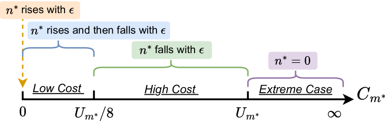
Figure 5: The Optimal Prompt Number $n^{*}(m^{*},p_{m^{*}},\epsilon)$ of Homogeneous Users with Different Ambiguity $\epsilon$ under $p^{*}_{m^{*}}$ in (11a).

Through Corollary 1, Proposition 3 highlights the impact of prompt ambiguity $\epsilon\in(0,1)$ on the platform’s optimal payoff, corresponding to that on users in Proposition 2.

Proposition 3.

The platform’s optimal payoff $\pi_{\textrm{platform}}^{*}(\boldsymbol{p}^{*})$ under homogeneous users decreases with ambiguity $\epsilon\in(0,1)$.

The complete proof of Proposition 3 is provided in appendix [24]. This proposition implies that prompt ambiguity has a detrimental effect on both the platform’s and users’ payoffs. Notably, an increase in prompt ambiguity $\epsilon$ does not guarantee a higher number of user prompts, as shown in Proposition 1. Even though the platform strategically optimizes the balance between prompt pricing and user prompt frequency, both parties experience diminishing optimal payoffs, creating a suboptimal outcome for all stakeholders.

IV-B The Optimal Prompt Pricing for Heterogeneous Users

Having analyzed the homogeneous case, we now address the more practical scenario of AIGC services with heterogeneous user prompt ambiguity. We begin by conducting a theoretical analysis of Problem 1 within this heterogeneous context, which is a multi-variable non-convex optimization (strongly NP-hard even in linear forms [29]). Then, we exploit the interaction between user behavior, GAI models, and prompt pricing to design an efficient algorithm for solving it.

IV-B1 Theoretical Analysis

Based on heterogeneous users’ optimal prompt strategy in Theorem 1, we first investigate the payoff maximization for the platform under any single model $m\in\mathcal{M}$. With Proposition 1 and Lemma 2, we reformulate such a problem into an unconstrained piecewise optimization in Problem 2, where $\lambda_{1}(k)\in(0,1)$ and $\lambda_{2}(k)\in(0,1)$ are the implicit solutions of equation $\epsilon^{k-1}(1-\epsilon)U_{m}=p_{m}$ with $\lambda_{1}(k)\leq\lambda_{2}(k)$, and upper bound $\bar{n}^{*}(m)$ in (9).

This transformation significantly reduces the complexity of optimal prompt pricing for single model. We illustrate this with Example 1, using a uniform distribution of prompt ambiguity.

Example 1 (Uniform Distribution of User Prompt Ambiguity).

For prompt ambiguity uniformly distributed over $[\epsilon_{\textrm{min}},\epsilon_{\textrm{max}}]$ where $\epsilon_{\textrm{min}}<\epsilon_{\textrm{max}}$:

• Problem 2 exhibits strict concavity on each piecewise segment $k\in[2,\bar{n}^{*}(m)]$.

• When $\epsilon_{\textrm{min}}=0$ and $C_{m}>0$, the optimal prompt price is $p^{*}_{m}=(U_{m}+C_{m})/2$.

Example 1 reveals that under uniform ambiguity distribution, the platform prioritizes users with lower ambiguity to maximize $\pi_{\textrm{platform}}(\boldsymbol{p})$. When the ambiguity distribution’s lower bound is zero, the optimal price $p^{*}_{m}$ depends solely on utility mapping $U_{m}$ and prompt cost $C_{m}$.

Following the prompt pricing for single GAI model, we extend our exploration to the entire model set $\mathcal{M}$ and incorporate users’ optimal model decisions derived in (III-A).

Input: prompt cost $C_{L}$ and $C_{H}$, utility mapping $U_{L}$ and $U_{H}$, user prompt ambiguity density function $f(\epsilon)$, and step size $\alpha$.

Output: the optimal prompt pricing $\boldsymbol{p}^{*}=\{p_{L}^{*},p_{H}^{*}\}$ and resultant payoff $\pi_{\textrm{platform}}^{*}$.

1 $\pi_{\textrm{platform}}^{*}=0$;

2 for $p_{L}=C_{L}:\alpha:U_{L}$ do

3   Derive $\bar{p}_{H}(M_{L},\epsilon)$ in (IV-B1);

4    Construct $\tilde{f}(\epsilon,p_{H})$ in (14b) and $G(p_{H})$ in (IV-B2);

5    $\hat{p}_{H}=\{x\in[C_{H},\bar{p}_{H}(M_{L},0)]:\partial G(x)/\partial x=0\}$;

6    $p_{H}=\operatorname*{argmax}_{x\in\{C_{H},\hat{p}_{H},\bar{p}_{H}(M_{L},0)\}}G(x)$;

7    if $\pi_{\textrm{platform}}(p_{L},p_{H})\geq\pi^{*}_{\textrm{platform}}$ then

8      $\boldsymbol{p}^{*}=\{p_{L},p_{H}\}$;

9       $\pi^{*}_{\textrm{platform}}=\pi_{\textrm{platform}}(p_{L},p_{H})$;

10   

11Return $\boldsymbol{p}^{*}$ and $\pi^{*}_{\textrm{platform}}$;

Algorithm 1 The Optimal Prompt Pricing (OPP).

Specifically, for any two models $m$ and $m^{\prime}$ in $\mathcal{M}$, we establish upper bound $\bar{p}_{m}(m^{\prime},\epsilon)$ on prompt price $p_{m}$ such that users with prompt ambiguity $\epsilon\in(0,1)$ will prefer model $m\in\mathcal{M}$ over $m^{\prime}\in\mathcal{M}$, and vice versa, expressed as below:

$$\bar{p}_{m}(m^{\prime},\epsilon)= \left[(1-\epsilon^{\tau(m,m^{\prime},\epsilon)})\cdot U_{m}+n^{*}(m^{\prime},p_{m^{\prime}},\epsilon)\cdot p_{m^{\prime}}\right.$$

$$-\left.(1-\epsilon^{n^{*}(m^{\prime},p_{m^{\prime}},\epsilon)})\cdot U_{m^{\prime}}\right]\cdot\frac{1}{\tau(m,m^{\prime},\epsilon)},$$ (12)

where $n^{*}(m^{\prime},p_{m^{\prime}},\epsilon)$ is in Theorem 1 and $\tau(m,m^{\prime},\epsilon)$ is:

$$\tau(m,m^{\prime},\epsilon)= \min\{k\in\mathbb{N}^{+}:(1-\epsilon^{n^{*}})\cdot U_{m^{\prime}}-n^{*}\cdot p_{m^{\prime}}$$

$$<(1-\epsilon^{k})\cdot U_{m}-k\epsilon^{k}(1-\epsilon)\cdot U_{m}\}.$$ (13)

From (IV-B1), the optimal prompt pricing involves multi-level interactions with heterogeneous users’ prompt strategy and model decision, especially given model set $\mathcal{M}$ and ambiguity distribution $f(\epsilon)$. This interrelation introduces non-convexity and significant computational complexity, making it difficult to derive a closed-form solution in general scenarios. Hence, we next aim to develop an efficient algorithm for Problem 1.

IV-B2 Algorithm Design

To address Problem 1, we develop the Optimal Prompt Pricing (OPP) algorithm (Algorithm 1) through systematic decomposition into tractable sub-problems. Our approach, inspired by finite element methods [30, 31, 32], enhances computational efficiency by reducing the search space to a single dimension compared to exhaustive search. The algorithm integrates price upper bounds and strategically partitions the ambiguity distribution based on user decisions.

Workflow of Algorithm 1: Given prompt cost and utility mapping of GAI models in set $\mathcal{M}=\{M_{L},M_{H}\}$, and user prompt ambiguity density function $f(\epsilon)$, we identify the upper bound $\bar{p}_{H}(M_{L},\epsilon)$ in (IV-B1), corresponding to prompt price $p_{L}$ of model $M_{L}$ (Line 2-3). Then, we partition $f(\epsilon)$ according to the optimal model decisions of heterogeneous users in AIGC services, formulated as a function of prompt price $p_{H}$:

$$\tilde{f}(\epsilon,p_{H})= f(\epsilon), p_{H}\leq\bar{p}_{H}(M_{L},\epsilon),$$ if (14a)

$$\tilde{f}(\epsilon,p_{H})= 0, p_{H}>\bar{p}_{H}(M_{L},\epsilon)$$ if . (14b)

Using revised ambiguity density function $\tilde{f}(\epsilon,p_{H})$ from (14b), we construct $G(p_{H})$ in (IV-B2), aligning it with optimizing price $p_{H}$ for platform payoff maximization (Line 4):

$$G(p_{H})= \int_{0}^{1}\tilde{f}(\epsilon,p_{H})\cdot\left[(p_{H}-C_{H})\cdot n^{*}(M_{H},p_{H},\epsilon)\right.$$

$$\left.-(p_{L}-C_{L})\cdot n^{*}(M_{L},p_{L},\epsilon)\right]d\epsilon.$$ (15)

Through the preceding transformation and simplification, we derive the optimal prompt price $p^{*}_{H}$ for any given $p_{L}$ of model $M_{L}$ (Line 5-6). By iteratively updating the prompt pricing mechanism, the OPP algorithm ultimately outputs the optimal one and resultant payoff for the platform (Lines 7-9).

V Experimental Evaluation

This section outlines the experimental setup and presents results validating the theoretical analysis of user strategies and prompt pricing, highlighting their impact on platform payoff.

V-A Experimental Setup

We adopt a character-level GPT-like model [23], with $21$ million parameters and a block size of $256$ to simulate practical AIGC services. Following [20, 21, 22], we generate synthetic language data for training using a doubly-embedded Markov chain model. To simulate varying user prompt ambiguity $\epsilon$, we inject noise into the transition matrix and uniformly distribute prompt ambiguity within $[\epsilon_{\textrm{min}},\epsilon_{\textrm{max}}]$. We scale system factors proportionally to GAI models’ utility to analyze their interactions. Due to the page limit, we include additional results, such as those for different ambiguity distributions, in appendix [24], where the insights are similar.

V-B The User’s Optimal Strategy and Expected Payoff

V-B1 The User’s Optimal Strategy

Figure 6 illustrates how prompt ambiguity $\epsilon$ and the number of prompts $n$ influence the GAI model’s output and the user’s optimal strategy. In Figure 6(a), the KL divergence [33] between the model’s output and the user’s true intention increases with ambiguity $\epsilon$ but decreases as the number of prompts $n$ grows. When $\epsilon=0$ (no ambiguity), the divergence is minimal, aligning with the analysis in Section II-B. Figure 6(b) shows that users with moderate ambiguity tend to issue more prompts, while a higher prompt price $p_{m}$ reduces the number of prompts.

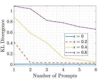
(a) Prompt Number and Ambiguity

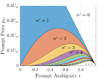
(b) Optimal Number $n^{*}(m,p_{m},\epsilon)$

Figure 6: The User’s Optimal Utilization Strategy.

V-B2 The User’s Optimal Payoff

Figure 7 demonstrates how the user’s optimal payoff $\pi^{*}_{\textrm{user}}$, given the model’s optimal decision $s^{*}$, varies with ambiguity $\epsilon$ and prompt price $p_{s^{*}}$. As seen in Figure 7(a), ambiguity $\epsilon$ determines the price threshold $p_{s^{*}}$ at which the user achieves a positive payoff and is willing to purchase the AIGC service. Figure 7(b) reveals that as $p_{s^{*}}$ increases, the user’s payoff $\pi^{*}_{\textrm{user}}$ declines despite strategic adjustments in utilization. Notably, higher ambiguity $\epsilon$ leads to a sharper reduction in the user’s optimal payoff.

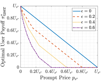
(a) Payoff $\pi^{*}_{\textrm{user}}$ and Price $p_{s^{*}}$

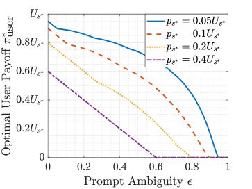
(b) Payoff $\pi^{*}_{\textrm{user}}$ and Ambiguity $\epsilon$

Figure 7: The User’s Optimal Expected Payoff.

V-C The Platform’s Optimal Pricing and Expected Payoff

V-C1 The Platform’s Optimal Pricing

Figure 8 examines the platform’s optimal prompt price $p^{*}_{m^{*}}$ for model $m^{*}$ under varying prompt ambiguities $\epsilon$ and the resulting user strategy $n^{*}(m^{*},p^{*}_{m^{*}},\epsilon)$. In Figure 8(a), the optimal pricing behavior depends on prompt cost $C_{m^{*}}$ and ambiguity $\epsilon$. Initially, as $\epsilon$ increases, the platform lowers $p^{*}_{m^{*}}$ to encourage more prompts and maximize its payoff. However, beyond a critical ambiguity threshold (e.g., $\epsilon=0.86$ for $C_{m^{*}}=0.1U_{m^{*}}$, marked by the red dashed line in both subfigures), the platform shifts to increasing $p^{*}_{m^{*}}$, prioritizing higher prices over more frequent prompts for payoff maximization.

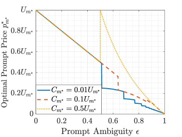
(a) Price $p^{*}_{m^{*}}$ and Ambiguity $\epsilon$

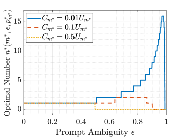
(b) $n^{*}(m^{*},p^{*}_{m^{*}},\epsilon)$ with $p^{*}_{m^{*}}$

Figure 8: The Platform’s Optimal Prompt Pricing.

V-C2 The Platform’s Optimal Payoff

Figure 9 compares the platform’s payoff under the OPP algorithm for model set $\mathcal{M}=\{M_{L},M_{H}\}$ with two benchmarks:

• Modified Utility-Based Pricing [34]: Adapts value-based pricing but neglects users’ strategic decisions across model sets.

• Modified Cost-Based Pricing [35]: Incorporates prompt costs but overlooks heterogeneous user strategies, limiting payoff optimization.

As shown in Figure 9, the platform’s payoff decreases with lower $\epsilon_{\text{min}}$ under all pricing mechanisms. While both OPP and utility-based pricing exhibit fluctuations due to user strategies, the OPP algorithm consistently outperforms benchmarks by leveraging users’ two-step decisions. It achieves at least $75.05\%$ and $31.72\%$ higher payoffs in the setups of Figures 9(a) and 9(b), respectively.

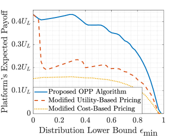
(a) Setup of $U_{H}=1.8U_{L}$, $C_{H}=0.04U_{L}$ and $C_{L}=0.02U_{L}$

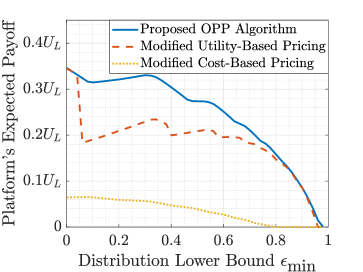
(b) Setup of $U_{H}=1.5U_{L}$, $C_{H}=0.06U_{L}$ and $C_{L}=0.02U_{L}$

Figure 9: The Platform’s Optimal Expected Payoff ($\epsilon_{\textrm{max}}=1$).

VI Conclusion

This paper provides the first study on strategic interactions between users and the platform in AIGC services. By introducing prompt ambiguity, we derive the optimal user utilization strategies and platform prompt pricing. Our exploration reveals complex interactions among decisions and system factors, where ambiguity adversely affects the payoff of both parties.

In future works, we will refine our theoretical analysis and OPP algorithm to support GAI models with more granular performance tiers, improving adaptability to diverse applications. Meanwhile, we will enhance our experiments with practical data sets and model-based agents.

References

- [1] A. Karapantelakis et al., “Generative AI in mobile networks: a survey,” Annals of Telecommunications, vol. 79, pp. 15–33, 2024.
- [2] “Monica - your ChatGPT AI assistant for anywhere,” https://monica.im/, accessed: 2025-1-24.
- [3] “Poe - fast, helpful AI chat,” https://poe.com, accessed: 2025-1-24.
- [4] OpenAI et al., “Gpt-4 technical report,” 2024.
- [5] OpenAI. (2023) Gpt-4 turbo (gpt-4o). Accessed: 2025-1-24. [Online]. Available: https://openai.com
- [6] Y. Cao et al., “A comprehensive survey of ai-generated content (aigc): A history of generative ai from gan to chatgpt,” 2023. [Online]. Available: https://arxiv.org/abs/2303.04226
- [7] H. Du et al., “Enabling ai-generated content services in wireless edge networks,” IEEE Wireless Communications, vol. 31, no. 3, pp. 226–234, 2024.
- [8] P. Dütting et al., “Mechanism design for large language models,” in ACM Web Conference, 2024, pp. 144–155.
- [9] M. Xu et al., “Sparks of gpts in edge intelligence for metaverse: Caching and inference for mobile aigc services,” 2023. [Online]. Available: https://arxiv.org/abs/2304.08782
- [10] Y. Liu et al., “Prosecutor: Protecting mobile aigc services on two-layer blockchain via reputation and contract theoretic approaches,” IEEE Transactions on Mobile Computing, vol. 23, no. 12, pp. 10 966–10 983, 2024.
- [11] H. Du et al., “Exploring collaborative distributed diffusion-based ai-generated content (aigc) in wireless networks,” IEEE Network, vol. 38, no. 3, pp. 178–186, 2024.
- [12] G. Liu et al., “Semantic communications for artificial intelligence generated content (aigc) toward effective content creation,” IEEE Network, vol. 38, no. 5, pp. 295–303, 2024.
- [13] J. Wu et al., “Ai-generated content (aigc): A survey,” 2023. [Online]. Available: https://arxiv.org/abs/2304.06632
- [14] C. Zhang et al., “A complete survey on generative ai (aigc): Is chatgpt from gpt-4 to gpt-5 all you need?” 2023. [Online]. Available: https://arxiv.org/abs/2303.11717
- [15] Y. Wang et al., “A survey on chatgpt: Ai–generated contents, challenges, and solutions,” IEEE Open Journal of the Computer Society, vol. 4, pp. 280–302, 2023.
- [16] “Bearly,” https://bearly.ai, accessed: 2025-1-24.
- [17] P. Sahoo et al., “A systematic survey of prompt engineering in large language models: Techniques and applications,” 2024. [Online]. Available: https://arxiv.org/abs/2402.07927
- [18] J. Wei et al., “Chain-of-thought prompting elicits reasoning in large language models,” in Advances in Neural Information Processing Systems, 2022, pp. 24 824–24 837.
- [19] Q. Dong et al., “A survey on in-context learning,” in Conference on Empirical Methods in Natural Language Processing, 2024, pp. 1107–1128.
- [20] Y. Zhou et al., “The mystery of in-context learning: A comprehensive survey on interpretation and analysis,” in Conference on Empirical Methods in Natural Language Processing, 2024, pp. 14 365–14 378.
- [21] S. M. Xie et al., “An explanation of in-context learning as implicit bayesian inference,” 2022. [Online]. Available: https://arxiv.org/abs/2111.02080
- [22] H. Jiang, “A latent space theory for emergent abilities in large language models,” 2023. [Online]. Available: https://arxiv.org/abs/2304.09960
- [23] A. Radford et al., “Improving language understanding by generative pre-training,” OpenAI, 2018.
- [24] X. Li et al., “Online appendix: Strategic prompt pricing for aigc services: A user-centric approach,” https://drive.google.com/drive/folders/1JFq3SoqNZwMC8I-yPEEHybfBOupp3OtJ?usp=sharing, accessed: 2025-1-24.
- [25] D. Patel and A. Ahmad, “The inference cost of search disruption – large language model cost analysis,” https://semianalysis.com/2023/02/09/the-inference-cost-of-search-disruption/, accessed: 2025-1-15.
- [26] R. Pieraccini and E. Levin, “Stochastic representation of semantic structure for speech understanding,” Speech Communication, vol. 11, no. 2, pp. 283–288, 1992.
- [27] S. Miller et al., “Hidden understanding models of natural language,” in Annual Meeting on Association for Computational Linguistics, 1994, pp. 25–32.
- [28] A. Mas-Colell et al., Microeconomic Theory. Oxford University Press, 1995.
- [29] P. Hansen et al., “New branch-and-bound rules for linear bilevel programming,” SIAM Journal on Scientific and Statistical Computing, vol. 13, no. 5, pp. 1194–1217, 1992.
- [30] W. Bangerth and R. Rannacher, Adaptive finite element methods for differential equations. Springer Science & Business Media, 2003.
- [31] B. Szabó and I. Babuška, Finite element analysis: Method, verification and validation. John Wiley & Sons, 2021.
- [32] I. Babuška and T. Strouboulis, The finite element method and its reliability. Oxford university press, 2001.
- [33] S. Kullback and R. A. Leibler, “On information and sufficiency,” The Annals of Mathematical Statistics, vol. 22, no. 1, pp. 79–86, 1951.
- [34] J. Pei, “A survey on data pricing: From economics to data science,” IEEE Transactions on Knowledge and Data Engineering, vol. 34, no. 10, pp. 4586–4608, 2022.
- [35] C. Courcoubetis and R. Weber, Pricing communication networks: Economics, technology and modelling. John Wiley & Sons, 2007.