Mie resonances in optical trapping: Their role in kinematics and back-action
Abstract
The heating rate plays a crucial role in the decoherence of the harmonic motion of an optically levitated nanoparticle. The values of this rate vary depending on both the scattering photon rate and the kinetic energy acquired through individual photon recoils. While the combined roles of these factors have been extensively studied, the energy transfer per recoil has not been explicitly examined. This energy transfer is often approximated using a linear dipole model with coefficients {1/5, 2/5, 7/5} which applies in the Rayleigh limit. In this work, we analyze the evolution of energy transfer per photon recoil for low-absorption dielectric nanospheres with diameters ranging from 2 nm to 500 nm. Using a far-field approximation, we demonstrate that the Kerker condition, which enhances the alignment between incident and scattered wavevectors, may significantly reduce the energy transferred per recoil. Although this reduction is counterbalanced by the increasing scattering rate, for an individual scattering event, the reduction of recoil suggests an intrinsic suppression of back-action. Our results reveal a potential enhancement in the accuracy of estimations in tabletop experiments involving Mie particles of the considered sizes and provide guidance for the selection of optimal probe sizes and materials. Our interpretation of recoil reduction as a manifestation of back-action suppression indicates the potential for quantum nondemolition (QND) measurements by tailoring scattered radiation patterns with metamaterials.
I Introduction
Optical levitation has shown to be a transformative approach in precision metrology, enabling groundbreaking advancements in weak force sensing [1, 2, 3, 4, 5, 6, 7]. Employing levitated systems allows for exploring fundamental questions in physics, potentially including dark matter detection [8, 9, 10], quantum measurement projection (collapse) models [11], and realization of microscopic entanglement [12, 13, 14]. These advances have stimulated intensive investigations on improving experimental accuracy in optical levitation experiments, expanding the boundaries of quantum control and noise reduction.
The key process limiting the experimental accuracy is the decoherence of the harmonic motion of the levitated oscillator. In high-vacuum environments, the dominant contribution to decoherence arises from the heating rate induced by photon recoil associated with scattering. This process significantly impacts the imprecision and back-action noises, collectively considered as the quantum noise level in experiments [15]. Due to its significance, the recoil heating rate has been extensively studied for dipolar scatterers in the Rayleigh regime [16, 17, 18]. Recent efforts stepped beyond this regime and determined the recoil heating rate in the intermediate and Mie regimes where levitated objects are larger. The importance of such studies relies on the link between the magnitude of recoil heating rate and the size parameter of scatterers as studied for silica [19, 20] and silicon [21].
Using Mie particles in levitation experiments introduces new opportunities and challenges. This is because the intrinsic characteristics of these particles give rise to electromagnetic resonances that alter the radiation patterns of scattered light. A particular example of such resonances was theoretically considered by Kerker, predicting the suppression of backscattering [22, 23]. Generally referred to as Mie resonances [24], these resonances affect the scattering characteristics, which exhibit exciting prospects for controlling levitated systems. Suggesting an auxiliary means, they can be used for stable particle confinement at a lower trapping potential by controlling attraction or repulsion forces as desired [25, 26, 27, 21, 28], and enhancing the detection efficiency by adjusting information radiation pattern [20, 29].
Despite often being treated as a single parameter, the recoil heating rate arises from two distinct contributions: (1) the average kinetic energy transfer per photon scattering event, which is a kinematic process, and (2) the photon scattering rate, which is a temporal process. These two components are of inherently different physical nature and offer unique possibilities for experimental control. For instance, controlling the radiation pattern via self-interference, achieved through spherical mirrors, has been proposed to reduce back-action noise for dipolar scatterers [30, 31]. Hence, achieving independent control over these two contributions can play a critical role in minimizing decoherence and enhancing the performance of levitated systems.
In this work, we present a detailed numerical investigation of the kinematic component of the recoil heating rate for Mie particles that satisfy the first Kerker condition [32, 33]. To gain qualitative insights, we analyze spherical particles made of silica, diamond, and silicon with diameters ranging from 2 nm to 500 nm. Trapping configurations were chosen to emulate typical experimental setups, utilizing unidirectional beams with either linear or radial polarization. Our findings reveal a considerable redistribution of the kinetic energy across translational degrees of freedom as particles approach the Kerker condition. This behavior underscores the significance of controlling scatterer radiation directivity for transferred energy redistribution and provides practical guidelines for selecting particle sizes, thereby delineating the limits of the Rayleigh approximation in the kinematic sense.
This work is structured as follows. In Sec. II, we cover the role of the kinematic component in the formation of the quantum noise, discuss its traditional consideration, and link it to the back-action effect. Section III introduces a generic approach to compute kinematic components in far-field approximation applicable to the beams beyond the paraxial regime. Numerical results for several beam modes are presented in Sec. IV, where we also provide the discussion and offer related remarks. Finally, we summarize our findings in Sec. V.
II Motivation
The modern description of displacement measurement accuracy unavoidably faces quantum limitations. These limits are postulated by Heisenberg’s uncertainty principle and set an upper bound on experimental accuracy, commonly dubbed standard quantum limit (SQL). In the case of the harmonic oscillator, the SQL is discussed in terms of the power spectral density of the total quantum noise (), where is the consisting frequency. This quantity in its complete form reads (see, e.g., [34, 15])
| (1) |
Here, is linked to the imprecision noise arising due to shot noise inherent to the measuring apparatus, e.g., uncontrolled fluctuations of the number of photons or electrons in the probing tool. The second term () accounts for the back-action noise, which is related to the uncertainty measurement of the momentum (or field amplitude) due to uncontrollable recoil impinged on the observed object during the interaction with the probe. The third term () represents the contribution originating from the cross-correlation between the previous two types of noises, where fluctuations in the probe correlate to back-action and vice versa; see details in [34]. In the following, we limit the discussion to the uncorrelated system, where the cross-correlation term () vanishes. Subsequently, for this general (uncorrelated) case, the total quantum noise becomes [35, 34]
| (2) |
Here, stands for the achievable SQL magnitude, and is the coupling constant characterizing the extent to which the probe affects the observed system during the measurement process.
In the field of optical trapping, for the mechanical oscillator with mass and resonant frequency , parameters and in Eq. (2) read [15]
| (3) |
Here, is related to the mechanical susceptibility as and denotes the mean displacement of the oscillator in the ground state . The rate (a.k.a. “recoil heating rate” [16, 20], “recoil rate” [36], “phonon heating rate” [5], “rate of occupation number increase” [19]) is given as the inverse time required for the incident light to heat the mechanical oscillator by the energy of one phonon due to the recoil at scattering. For the elastic scattering process, this rate is given by (see, e.g.,[19] and Sec. 4.2 in [37])
| (4) |
where sets the rate of scattered photons (the number of scattering events per second), denotes the focal intensity of light, is the scattering cross-section and is the light frequency. Here, is the kinetic energy of the oscillator equal to the energy of the incident photon with the wave number , i.e., . The coefficient accounts for the average fraction of the kinetic energy distributed over three transnational degrees of motion, i.e., , after the single scattering event. In the other formulation is the dispersion fraction of mechanical momentum difference between the incident and scattered photons’ momenta with wavenumber (see, e.g., [38] and Sec. 4.2 in [37]), where denotes a unit vector along . Since the heating rate characterizes the decoherence introduced by trapping light to the measurement, its magnitude draws substantial interest (see, e.g., [19, 20]). The studies treat as a solid parameter with no explicit distinction between the consisting components in Eq. (4). In the current work, we focus on the quantity characterizing the kinetic energy variation of the oscillator interacting with the incident photon during an individual scattering event. We primarily focus on the magnitude of the parameter characterizing the scattering photon recoil associated with the back-action mechanism.
In general, the coefficient appears as a result of the calculation of the autocorrelation function of the force impinged onto the trapped harmonic oscillator (see, e.g., supplementary to [16], Sec. 4.2 in [37], and [31]), which is needed for deriving the back-action or imprecision noises. For the plane incident wave propagating along the direction -axis and polarized along the -direction, i.e., , the parameter is written as (see, e.g., [39, 19]):
| (5) |
where is the th component of a unit vector along the wavevector of the scattered photon propagation and the angle brackets stands for the averaging over full solid angle . The extra unity in the z-component appears due to the radiation pressure caused by the momentum of the incident photon permanently applied to the oscillator. Assuming the scatterer to be a linear dipole with differential power ( is the polar angle counted from the negative direction of z, and is the azimuthal angle in the plane perpendicular to z, see Fig. S1 in the Supplemental Materials (SM) [40]), where averaging over the full solid angle results in for ; see, e.g., [38, 17, 39, 19, 15]. Attempts to extend these results to the case of the trapping Gaussian beam focused with high numerical aperture () leads to rewriting as [17]
| (6) |
where is an effective parameter characterizing the total phase of the incident beam along the propagation direction z-axis, where is the Gouy phase, at the position of a trapped particle; see [17], Sec. 3.3 in [41]. In experiments tracking the displacement of the scatterer’s position, the phase plays a central role, as it is imprinted in the scattered light, making position retrieval possible [42, 43, 17]. The factor is included in the relation , between scattered power , and time-averaged radiation pressure force exerted along the beam’s propagation direction, and the constant is the speed of light [17]. On the other hand, the radiation pressure force can be canonically written as (see, e.g., Sec. 14.4 in [44] and Sec. 16.10 in [45]), that offers the physical interpretation of . The parameter is an effective propagation constant which represents the effective longitudinal component of the wavevector characterizing the incident Gaussian beam; see also [46] for details.
For our further analysis, it is important to note that from eq.(6) can be expressed solely in terms of the angular distributions of the incident and scattered fields. Such, the photon recoil force for an active emitter (scattering without absorption) can be described via the scattering angle , taken as an azimuthal angle to the z-axis. This dependence can be formulated in terms of , which is commonly referred to as the asymmetry factor (see, e.g., [47, 48, 49] and Sec. 3.11 [50]); see SM [40] for details. On the other hand, for a passive scatterer (absorption without scattering) the parameter can be defined as the mean longitudinal projection of the wavevector , i.e. , averaged over the angular spectra function characterizing incident field (see [47, 48, 49]). These relationships suggest that the parameter can be expressed in terms of the asymmetry factors, offering an alternative calculation method compared to the approach based on the Gouy phase approximation. Specifically, it can be defined as , which yields from eq. (6), since when averaged dipole scattering function .
Obtaining in a plane wave approximation enables us to account for the impact of the Gaussian beam along the propagation direction. However, the approach is limited to the case of the incident plane wave with the parameter relevant to the beam propagation direction z. In fact, modeling the incident field as a plane wave inherently neglects perturbations associated with the lateral momentum components and , which is only a valid approximation for the field distribution at the exact coordinate of the focus. This restriction causes and to remain unperturbed. Thus, if one has an interest in the general evolution of the parameters , and the components of the recoil heating , the general treatment beyond the incident plane wave approximation should be considered.
Given the central role of in defining and , directly influences the decoherence introduced by the trapping light. Modifying parameter can significantly influence back-action noise, thereby affecting measurement precision. Representing energy redistribution following an individual scattering event, characterizes the kinematic process. In this way, a better understanding of can shed light on the mechanism of reducing the undesired heating due to photon recoil and the corresponding reduction of the back-action effect. This viewpoint stimulates our interest in the evolution of depending on different setup conditions and various scatterers. In this regard, we have generalized the calculation presented in Sec. 4.2 in [37], which was obtained for the autocorrelation function of the instantaneous scattering force. The approach involves incorporating both the incident and scattered photon momenta, which results in the expression for back-action noise as , see the comment 111An alternative approach for calculating was recently proposed, see [31, 18]. It suggests calculating the force autocorrelation function in the frequency domain and utilizes Green’s functions and Fisher information representations.. The given averaging highlights the importance of the scattered radiation distribution as a weighted function, which directs our attention to its modification due to possible Mie resonances. In the subsequent section, we present the details of the calculation approach we followed.
III Methods
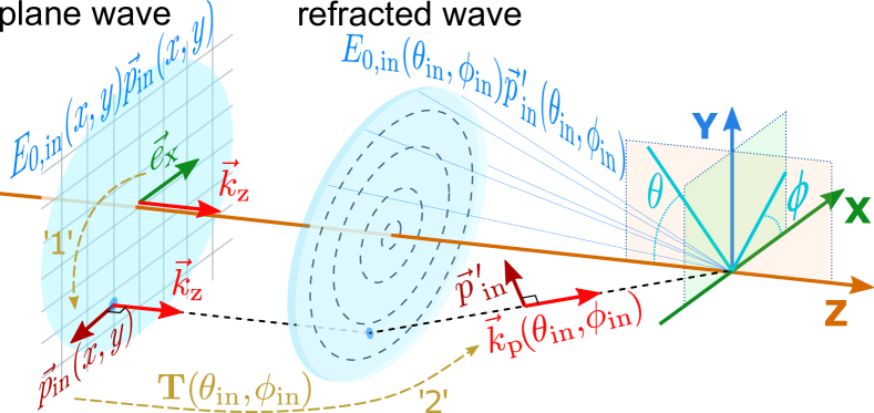
The calculation approach we follow in our work is based on the seminal work [38], which discusses the averaged kinetic energy acquired by the elementary scatterer (linear or circular dipole) under the influence of subsequent inelastic light scattering. Authors consider an incident plane wave with a wave vector and scattered light with wavevector and differential power (hereafter referred to as ) given in the far field, see illustration in Fig. 1. The resultant parameters was defined as , that can be written as (see [38, 19] and Sec. 4.2 in [37])
| (7) |
where is the probability density function corresponding to the normalized differential power distribution in the far field, and which integration is carried out over the full solid angle . Nevertheless, this commonly accepted formulation is a particular case in the sense that the incident beam is set to be a plane wave. Within this formulation, the wave vector propagation direction is given by angles () (“” stands for the “incident”) and the direction of the incident beam is determined by . Subsequently, the incident field polarized along direction can be defined in the k-space as (see, e.g., Sec. III.C in [52]). While this subtle detail has not been emphasized in many research studies, being aware of it allows us to tackle the problem in a more general way.
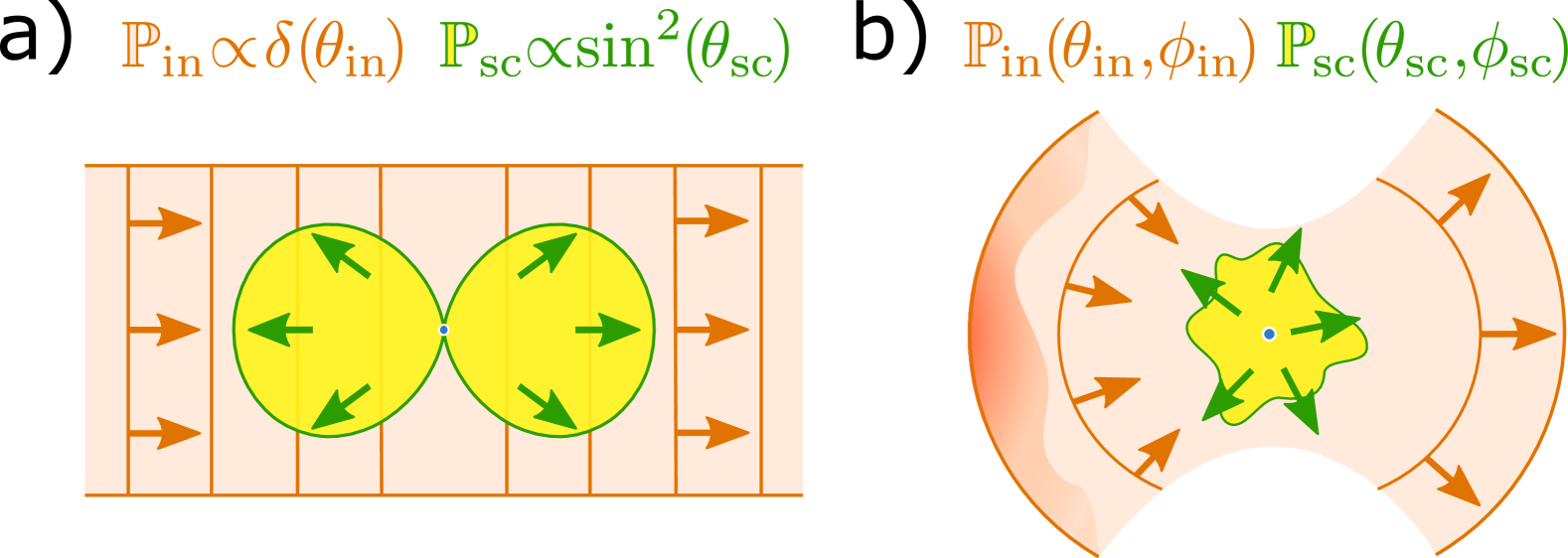
At the next stage, we generalize the above formulation by introducing the joint probability of two independent events characterizing incident photon income and scattered photon outcome. Each one is described by respective probability density function, and (see Fig. 1(b)), given by the normalized differential power as , with .
As a result, the general form for becomes
| (8) |
where and correspond to the scattering and extinction cross-sections, respectively. Further, we work in the frame of the absorptionless nanoparticles, claiming that we are in a regime where . The elements of the solid angles and in Eq. (8) are given in two independent spherical coordinate systems sharing the same basis vectors. Note that in Eq. (8), writing the total probability , as
| (9) |
we postulate the incident and scattering events are independent and identically distributed, i.e. angularly uncorrelated. Assuming in Eq. (8), we reproduce the canonical convention in Eq. (7) for the case of the incident plane wave, see, e.g., [19] and the supplementary to [16].
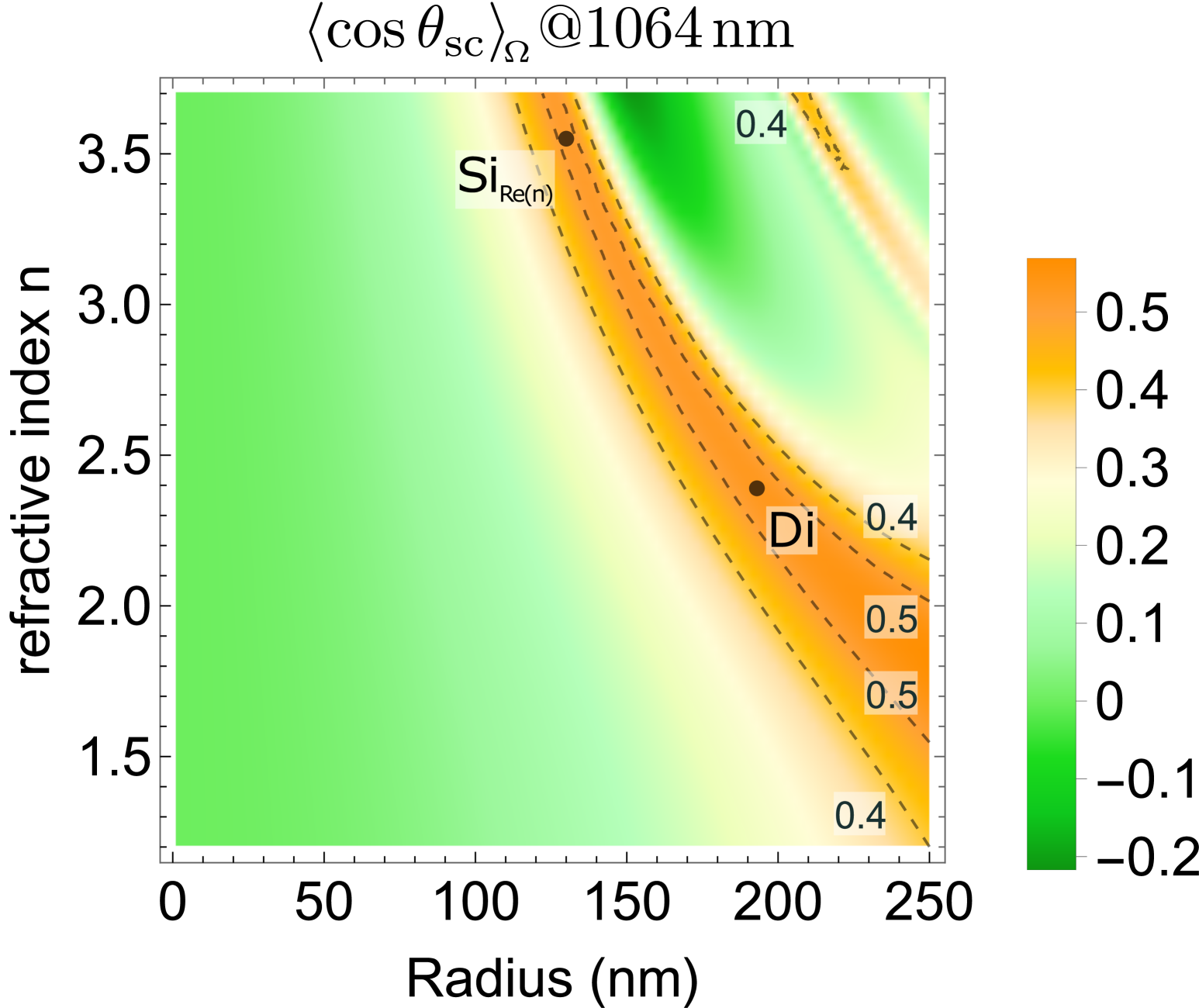
Analysis of the integral in Eq. (8) show that minimizing the requires the and to be co-directed. Since the incident beam is directed predominantly along the propagation direction z, the scattered light has to be directed along the positive z axis. This directivity magnitude can be characterized with the asymmetry factor . Being evaluated for the nanospheres of absorptionless materials with the refractive index , the asymmetry factor is presented in Fig. 2. The greater magnitude with can be achieved when the Kerker condition of the first type is met, see SM [40]. In the evaluation of Fig. 2, we assume that the radius of the sphere varies in the range and the wavelength of the incident light is . These parameters are used throughout the following work.
In order to implement the formulation given in Eq. (8), we assume two different distributions of the incident electric field determined in the far field, which defines (see SM [40]). The first one is a Gaussian beam with filling factor , and the second one is a superposition of Hermit-Gaussian modes and resulting in the radially polarized beam with . The choice of the filling factors magnitudes allows at least 95% of the total incident intensity to be collected by the focusing objective of the specified numerical aperture. The NA was chosen to be varied in the range of and defines the polar angle in the span covered by with and .
In turn, to calculate the function , we used an extended framework of the Mie theory obtained for linearly polarized incident plane wave, see SM [40]. The resultant scattering field depends on the radius of the dielectric scatterer, its refractive index, the vectorial electric field of the incident light, and the NA of the focusing objective. Defining all these parameters and substituting them in Eq. (8) allows us to obtain for the three translational motion degrees. Due to excessive computational expenses, the calculations were carried out on a grid with 154 points equidistantly distributed on the plane NA R (11 14). In the following section, we summarize results obtained for under the prescribed setup conditions and for scatterers made of three different materials.
IV Results and Discussion
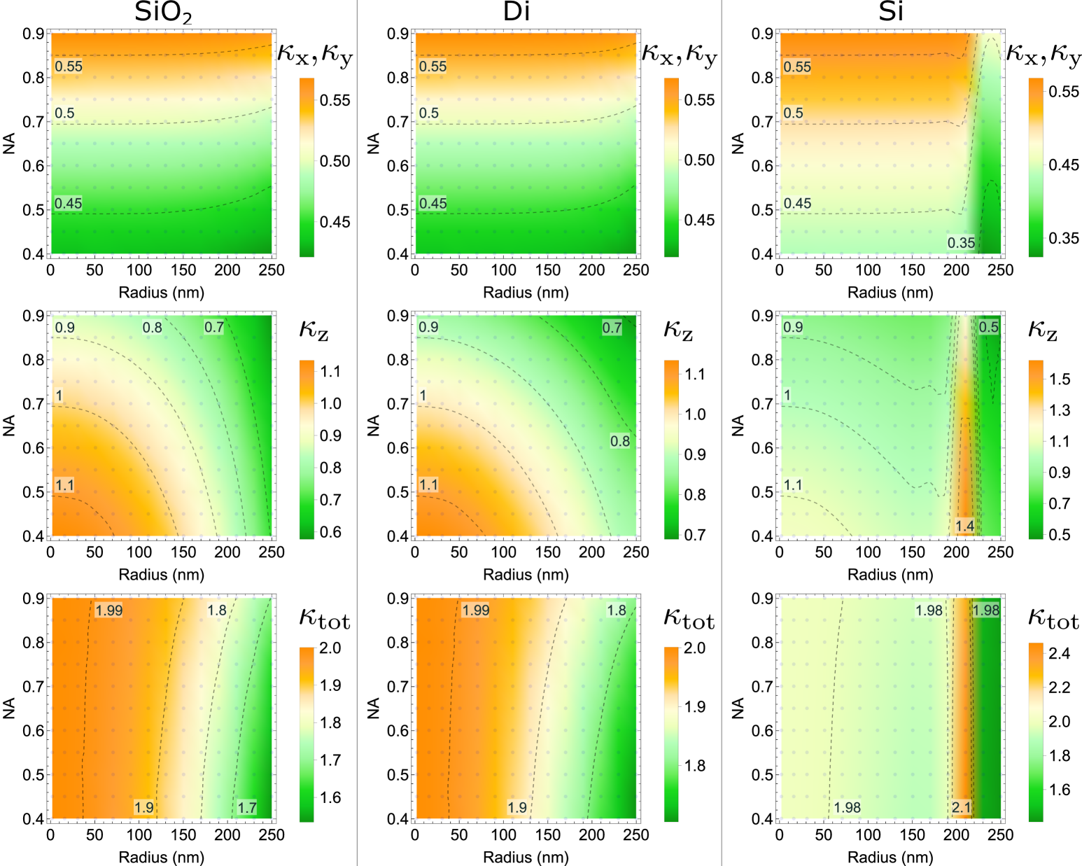
Having discussed our approach to calculate using various radiation probabilities, we here present our numerical results for . Our results consist of various distributions of and their sum – with , for three different cases: 1) silica “”, 2) diamond “Di”, and 3) silicon “Si” nanosphere, illuminated by linear Gaussian or radially polarized beams with wavelength of 1064 nm. The refractive indices of these three materials are almost equidistantly separated along the refractive index axis in Fig. 2. This allows us to extrapolate results obtained below for other materials with and negligibly low absorption when . The results for all three samples are presented in Fig. 3 and Fig. 4 in the left, middle, and right columns, respectively.
Incident linearly/circularly polarized light.
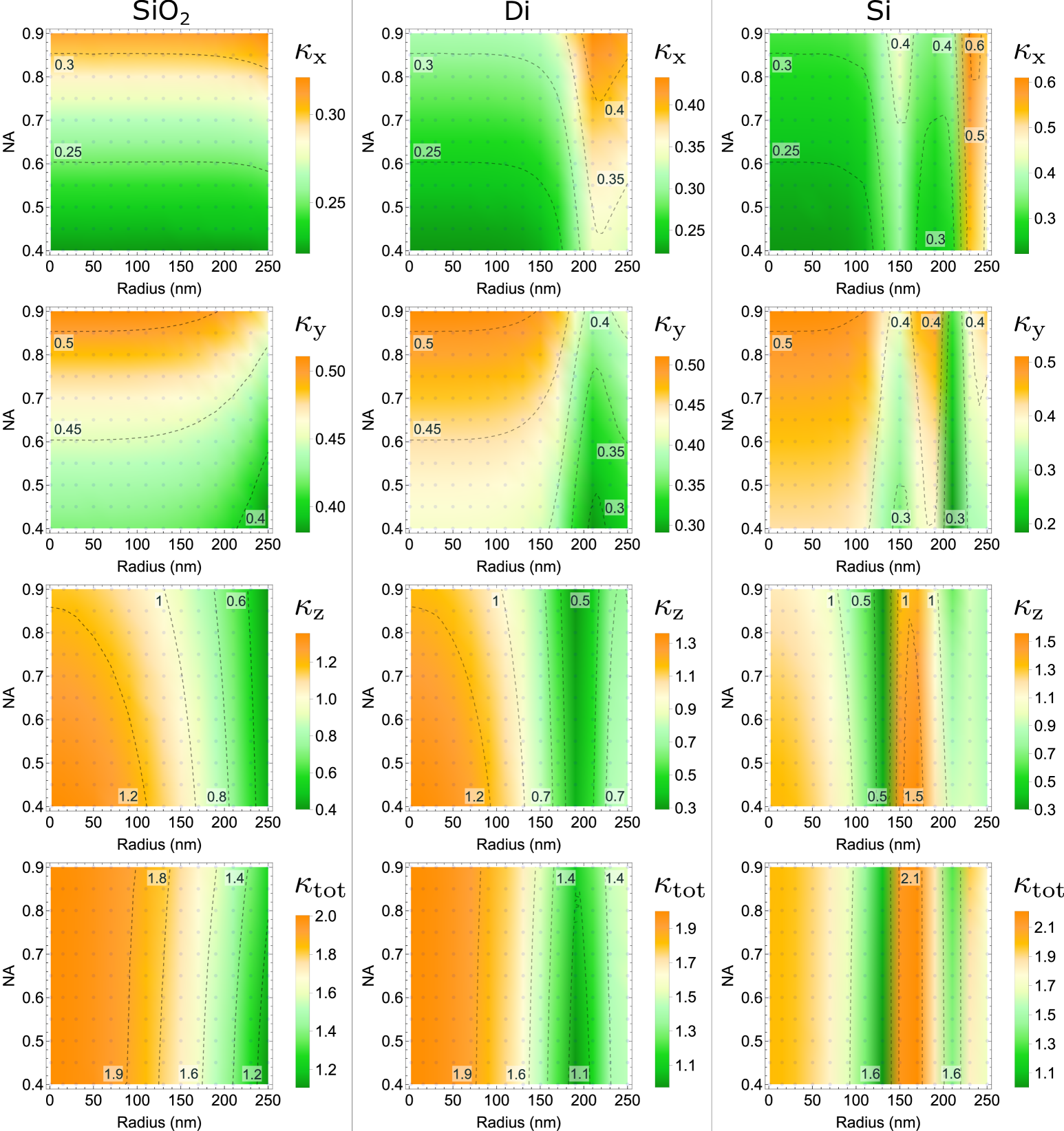
Figure 3 displays distributions of ’s and as a function of radius and NA for silica nanosphere illuminated with linearly polarized incident light. Due to the present axial symmetry in the x-y plane for the cases with incident circular polarization, the x or y components of can be evaluated as an averaged sum of and obtained for the incident linear polarization, i.e., . Hence, we merely focus on exploring our results for incident linear polarization.
The analysis of the distributions corresponding to silica in Fig. 3 reveals that and gradually decrease with increasing radius, exhibiting no anomalous behavior. The lateral components and remain predominantly constant and show negligible variation within the range , consistent with the Rayleigh approximation .
These observations can be attributed to the fact that a silica nanoparticle with a radius up to 250 nm does not exhibit significant changes in , as shown in Fig. 2, and the redistribution of radiation power with increasing radius (see Fig. S2 (a),(b) in the SM [40]) occurs gradually. Consequently, one can employ the parameters obtained for a radius of as a reliable approximation for a wide range of radius values.
In contrast to silica, the distributions of obtained for diamond and silicon display noticeable changes with radius growth (see Fig. 3 (middle and right columns)). Analyzing the total parameter , we observe its drastic drop near the radii corresponding to the maximally forward-directed light (about 130 nm for Si and 193 nm for diamond). For the z component, these observations are also evidently expressed, as the longitudinal (along z direction) radiation pattern is affected more with the growth of radius (see SM [40]). Besides, Fig. 3 exhibits that when approaching the size of the minima dip for , and continue their change, and extremum of these changes lay slightly further to the expected value (about 150 nm and 230 nm, for Si and diamond, correspondingly). This observation is attributed to the redistribution of radiation between the x and y directions, as shown in Fig. S2(d) in the SM [40], when the Kerker condition is satisfied. To illustrate this redistribution, we calculated characteristic radiation patterns for silicon nanoparticles with radii of nm. This allows us to understand the “overflowing” between the magnitudes of and , which becomes pronounced around .
Radially polarized incident light.
For the case of the radially polarized incident light, we obtain the results given in Fig. 4. As in the case of circular polarization, due to the axial symmetry of the vector incident field, distributions and are the same. Besides, we observe remarkable changes in comparison with the incident linear (circular) Gaussian beam. The most evident one is the shift of the radius, which provides the highest forward scattering. The distributions obtained for Si show that the characteristic dips of are shifted along the radius axes away from 130-150 nm by approximately 100 nm. As to the case of diamond, these changes occur beyond the maximal radius we consider in our work and are not shown in Fig. 4. As can be seen, the lateral distributions have no significant changes in the broader range of radii compared to the results obtained for linearly polarized light. Moreover, the distribution of obtained for silicon points to negligible variation over a broad range of radii . These observations might be useful for justification of the dipole approximation when applied to large nanospheres made of silicon or materials with similar refractive indices.
The characteristic shift of the forward scattering condition towards the higher radii is due to excitation of the anapole modes [53, 54, 55]. Due to the superposition of the plane waves at the focus, the excitation of dipoles (electric and magnetic) modes is significantly suppressed, and the resonance of higher-order magnetic and electric modes contributes to the radiation, see Fig. S2 (c) in the SM [40]. For the quadrupole modes, we expect the conditions of significant forward scattering to be satisfied when (see SM [40]) and calculations show that it occurs near for silicon, and for diamond.
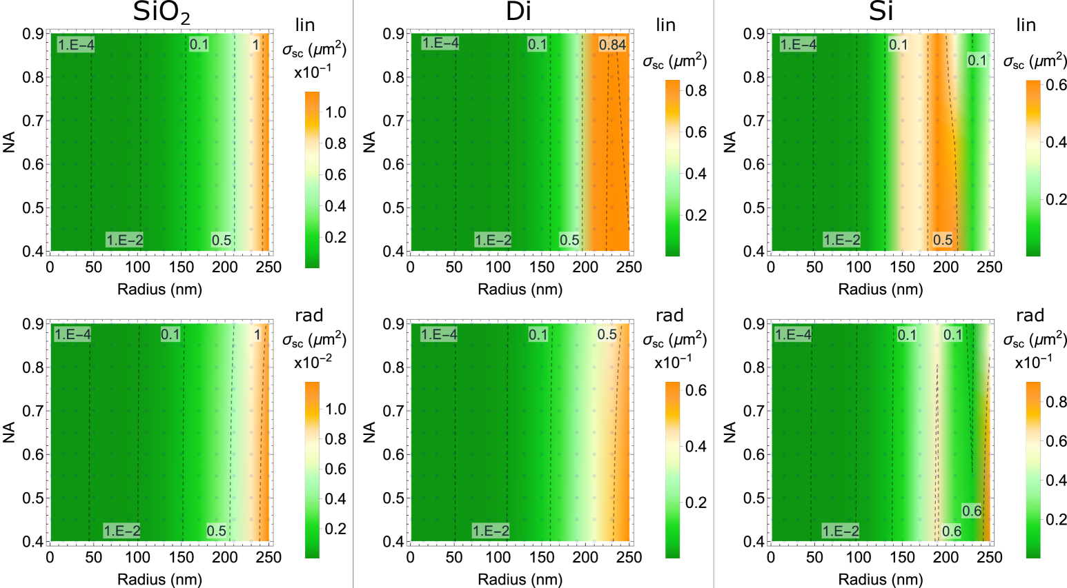
So far, we have focused on the computation of the mechanical recoil parameter , central to describing recoil heating effects. While previous studies often approach the recoil heating rate as a product of and the scattering cross-section [19, 20, 15], our methodology isolates for detailed evaluation. Alongside , our calculation framework naturally determines , the results of which are presented in the SM [40], showing significant growth over the given range of radii. The separation of these contributions allows for a more nuanced understanding of the kinematic processes described by , independent of the scattering rate , which is defined via .
The variation of the cross-section () with radius (see Fig. S5 in the SM [40]) dominates over the variation of . As a result, the characteristic dips in the contributing to are not distinctive. Although increasing ultimately enhances decoherence, which degrades experimental sensitivity, the nature of also allows to be discussed in terms of “signal redundancy”. Since the scattering rate in Eq.(4) is proportional to , the growth of can be compensated by reducing the trapping power to keep constant. This makes solely sensitive to the kinematic component , allowing the reduction of to be interpreted as a reduction of back-action in general. On the other hand, the increased scattering rate can improve the reliability of feedback cooling systems by reducing the acquisition time required for precise motion tracking, thereby increasing the rate of feedback. Consequently, the system becomes more resilient to noise and instability, improving cooling performance. The discussed redundancy offers a potential advantage in applications tracking fast perturbations where frequent interrogation of the oscillator’s position is essential. Despite this advantage, the overall degradation of , resulting from the dominant growth of , introduces challenges for maintaining experimental sensitivity.
To this extent, we consider the individual, although spatially averaged, scattering event, which highlights the pure kinematic nature of the momentum uncertainty evolution during a photon recoil, excluding the temporal aspect of recoil heating expressed in the rate of such events. Our computational approach provides accurate values for , enabling its independent assessment.
Final remarks.
The presented findings reveal a natural increase in forward scattering, which occurs without the need for auxiliary components and leads to a recoil reduction. We interpret this reduction in recoil as a decrease in back-action at the level of individual scattering events. Our analysis focuses on an optical setup with a single-pass trapping beam, where directivity plays a crucial role. This system represents a particular realization of optical trapping. In contrast, trapping systems based on standing waves are fundamentally different. Since a standing wave forms from two counter-propagating waves, forward and backward directions become indistinguishable, making the concept of the mere use of forward scattering inapplicable. As a result, our findings do not extend to such systems.
The reduction of recoil was considered under idealized conditions, assuming zero absorption. However, in real experiments, one must account for the heating of the trapping object in experimental setups (see, e.g., [56]). As pointed out in Sec. 4.1 and 4.5 in [57] and [58], the amount of the incident power and the rise of temperature of the trapped object both affect the refractive index of the sphere’s material. The effective refractive index with the neglected nonlinear refractive index component can be written in the following form
| (10) |
where is the thermo-optic coefficient and is the temperature variation. Such dependence on the temperature assumes altering the conditional radius to obtain the required directivity maxima approaching the Kerker condition. This point means that the choice of the radius of the trapped nanoparticles sample allows for some preliminary corrections in the choice of radii in practice. In the case of silicon, we estimate the thermo-optic coefficient comparing refractive indexes obtained for 300 K and 500 K (see [59, 60]) and found it to be . The calculations of Eq. (S7) with this correction coefficient suggest that a silicon nanoparticle illuminated with linearly polarized light and heated up to 1000 K shifts the corresponding radius of expected maximal directivity from nm to nm. On the other hand, the estimations of the scattering rate show that the assumption that made in Sec. III is expected to hold for the silicon at room conditions, to which we obtain , weakens for heated material resulting in at that only would facilitate further heating. These estimations lead to the fact that minimizing the back-action effect might not be easily realized for the optical trapping experiments. However, it can still be applicable for the experiments utilizing the so-called dark potentials (see, e.g., [61, 62]), where the incident light power can be drastically reduced for only detection needs excluding trapping.
As our final remark, we note that the opportunity to enhance forward scattering has consequences manifested as increased the scattering cross-section. The connection between directivity and scattering cross-section can be understood in terms of the optical theorem, i.e., the growth of amplitude of the forward scattered light, characterized by directivity, leads to the rise of the scattering cross-section. Thus, within the scope of this work, the following potential avenues for future research can be highlighted: 1) obtaining the extreme directive scattering source with the possibility to vary its radius on demand, and 2) mitigating the dependence of the scattering cross-section on the forward scattered light. The first one might be achieved with further developments in Mie-tronics (see, e.g., [63, 64]) and engineering new scatterers and metamaterials (see, e.g., [65, 66]). As an example, the high directivity of a single nanosphere was obtained by adding extra dielectric shells (dielectric layers) (see, e.g., [67],[68]), or slight deformation of a sphere’s shape adding a notch (see, e.g., [69]). Concerning the second point, the optical theorem is based on the reciprocity and energy conservation law, weakening the optical theorem would require violation of one of these two. Hence, the perspectives to overcome this correlation can be found by involving non-Hermitian processes.
V Conclusion
We have discussed the connection between the directivity achieved at scattering from Mie particles and the kinematic recoil component concerning optical levitation. The problem was treated in far-field representation using plane wave decomposition. We have presented the general discussion approach used to obtain the scattered field corresponding to the broad range of focusing NA relevant to tabletop experiments for finding corresponding recoil momenta uncertainty associated with the back-action of an individual scattering event.
For the particular examples of silica, diamond, and silicon nanospheres with diameters up to 500 nm, we studied the role of the satisfied Kerker condition in reducing the kinetic energy transferred to the trapped particles. Although we limited ourselves to particular materials, our conclusions may go beyond these particular cases and allow for an understanding of general tendencies for low-absorption materials with a wide range of refractive indices.
For the linearly focused Gaussian beam, the reduction of the total energy transferred to a particle exceeds 40% in comparison to the linear dipole, and exceeds 80% when comparing energy acquired for the direction along the beam propagation. The discussed reduction is mitigated by the faster rise of scattering cross-section and, hence, the recoil heating rate growth that causes a faster oscillator decoherence rate, preventing continuous measurement improvement. Nevertheless, the merits of gained directivity are shown for an individual scattering event; the obtained reduction of the emerged momentum uncertainty points to the advance toward the realization of “arbitrarily quick and arbitrarily accurate” type of measurement (see Sec. III.B in [70]), since the momentum of the oscillator is less perturbed by the measuring apparatus.
We have also considered the case of an incident radially polarized trapping beam. Due to the electric and magnetic dipole scattering modes suppression, the Kerker resonance was obtained for the quadrupole components, which required a significant increase of the nanosphere radii to fulfill this condition. For the studied radii range , the local high directivity was observed only for the silicon nanosphere at 227 nm.
Meeting the Kerker condition does not provide a perfect back-action reduction but a partial one. Nevertheless, showing distinguishable reduction of recoil momentum uncertainty due to naturally approached collinearity between incident and scattered light, our work opens further questions for further optimization approaches aimed to the further suppression of the recoil. Thus, the mechanism of reduction of the recoil should not be overlooked in the context of experimental investigations. Moreover, one may expect that modifying the forward scattering radiation caused by the inherent dielectric properties of the scatterer might be combined with the back-action suppression mechanism based on the self-interference discussed in [30, 31]. This combination has the potential to suppress back-action even further exceeding capabilities of each mechanism separately, and we leave this as an open question for further investigation.
The presented work highlights the prospects for further developments in metamaterials and metastructures to improve control over the scattering directivity of the optically levitated nanoparticles. In the limit, achieving collinearity between the incident and scattered photons results in the complete suppression of recoil scattering. This raises the natural question of whether such a configuration enables the quantum nondemolition measurements (see, e.g., [71, 70, 72, 73, 74]), which itself presents an exciting direction for future research.
Acknowledgments
V.S. acknowledges useful discussions and helpful communications with Andrea Aiello, Dmitry Bykov, Norbert Lindlein, Andrey Manchev, Florian Marquardt, Dmitriy Pokhabov, Colin Sheppard, Markus Sondermann, Sergey Vyatchanin. Technical suggestions on parallel computing from Räul González Garrido and Daniel Häupl are highly appreciated.
References
- Pesce et al. [2020] G. Pesce, P. H. Jones, O. M. Maragò, and G. Volpe, The European Physical Journal Plus 135, 949 (2020).
- Millen et al. [2020] J. Millen, T. S. Monteiro, R. Pettit, and A. N. Vamivakas, Reports on Progress in Physics 83, 026401 (2020).
- Gieseler et al. [2021] J. Gieseler, J. R. Gomez-Solano, A. Magazzù, I. Pérez Castillo, L. Perez Garcia, M. Gironella-Torrent, X. Viader-Godoy, F. Ritort, G. Pesce, A. V. Arzola, K. Volke-Sepulveda, and G. Volpe, Advances in Optics and Photonics 13, 74 (2021).
- Gonzalez-Ballestero et al. [2021] C. Gonzalez-Ballestero, M. Aspelmeyer, L. Novotny, R. Quidant, and O. Romero-Isart, Science 374, eabg3027 (2021).
- Winstone et al. [2023] G. Winstone, A. Grinin, M. Bhattacharya, A. A. Geraci, T. Li, P. J. Pauzauskie, and N. Vamivakas, (2023), arXiv:2307.11858 [quant-ph] .
- Volpe [2023] e. a. Volpe, Giovanni, Journal of Physics: Photonics 5, 022501 (2023).
- Jin et al. [2024] Y. Jin, K. Shen, P. Ju, and T. Li, (2024), arXiv:2407.12496 [physics.optics] .
- Monteiro et al. [2020] F. Monteiro, G. Afek, D. Carney, G. Krnjaic, J. Wang, and D. C. Moore, Physical Review Letters 125, 181102 (2020).
- Kalia et al. [2024] S. Kalia, D. Budker, D. F. J. Kimball, W. Ji, Z. Liu, A. O. Sushkov, C. Timberlake, H. Ulbricht, A. Vinante, and T. Wang, Physical Review D 110, 115029 (2024).
- Kilian et al. [2024] E. Kilian, M. Rademacher, J. M. H. Gosling, J. H. Iacoponi, F. Alder, M. Toroš, A. Pontin, C. Ghag, S. Bose, T. S. Monteiro, and P. F. Barker, AVS Quantum Science 6, 030503 (2024).
- Vinante et al. [2019] A. Vinante, A. Pontin, M. Rashid, M. Toros, P. F. Barker, and H. Ulbricht, Physical Review A 100, 012119 (2019).
- Poddubny et al. [2024] A. N. Poddubny, K. Winkler, B. A. Stickler, U. Delic, M. Aspelmeyer, and A. V. Zasedatelev, (2024), arXiv:2408.06251 [quant-ph] .
- Zambon et al. [2024] N. C. Zambon, M. Rossi, M. Frimmer, L. Novotny, C. Gonzalez-Ballestero, O. Romero-Isart, and A. Militaru, (2024), arXiv:2408.14439 [quant-ph] .
- Winkler et al. [2024] K. Winkler, A. V. Zasedatelev, B. A. Stickler, U. Delić, A. Deutschmann-Olek, and M. Aspelmeyer, (2024), arXiv:2408.07492 [quant-ph] .
- Gonzalez-Ballestero et al. [2023] C. Gonzalez-Ballestero, J. Zielińska, M. Rossi, A. Militaru, M. Frimmer, L. Novotny, P. Maurer, and O. Romero-Isart, PRX Quantum 4, 030331 (2023).
- Jain et al. [2016] V. Jain, J. Gieseler, C. Moritz, C. Dellago, R. Quidant, and L. Novotny, Physical Review Letters 116, 243601 (2016).
- Tebbenjohanns et al. [2019] F. Tebbenjohanns, M. Frimmer, and L. Novotny, Physical Review A 100, 043821 (2019).
- Abbassi [2024] M. A. Abbassi, (2024), arXiv:2404.12459 [physics.optics] .
- Seberson and Robicheaux [2020] T. Seberson and F. Robicheaux, Physical Review A 102, 33505 (2020).
- Maurer et al. [2023] P. Maurer, C. Gonzalez-Ballestero, and O. Romero-Isart, Phys. Rev. A 108, 033714 (2023).
- Lepeshov et al. [2023] S. Lepeshov, N. Meyer, P. Maurer, O. Romero-Isart, and R. Quidant, Physical Review Letters 130, 233601 (2023).
- Kerker et al. [1983] M. Kerker, D.-S. Wang, and C. L. Giles, Journal of the Optical Society of America 73, 765 (1983).
- Liu and Kivshar [2018] W. Liu and Y. S. Kivshar, Optics Express 26, 13085 (2018).
- Kivshar and Miroshnichenko [2017] Y. Kivshar and A. Miroshnichenko, Optics and Photonics News 28, 24 (2017).
- Stilgoe et al. [2008] A. B. Stilgoe, T. A. Nieminen, G. Knöener, N. R. Heckenberg, and H. Rubinsztein-Dunlop, Optics Express 16, 15039 (2008).
- Nieto-Vesperinas et al. [2010] M. Nieto-Vesperinas, R. Gomez-Medina, and J. J. Saenz, Journal of the Optical Society of America A 28, 54 (2010).
- Shilkin and Fedyanin [2022] D. A. Shilkin and A. A. Fedyanin, JETP Letters 115, 136 (2022).
- Mao et al. [2024] L. Mao, I. Toftul, S. Balendhran, M. Taha, Y. Kivshar, and S. Kruk, Laser & Photonics Reviews , 2400767 (2024).
- Wang et al. [2025] L. Wang, L.-M. Zhou, Y. Tian, L.-H. Liu, G.-C. Guo, Y. Zheng, and F.-W. Sun, Journal of the Optical Society of America B 42, 645 (2025).
- Weiser et al. [2025] Y. Weiser, T. Faorlin, L. Panzl, T. Lafenthaler, L. Dania, D. S. Bykov, T. Monz, R. Blatt, and G. Cerchiari, Physical Review A 111, 013503 (2025).
- Gajewski and Bateman [2024] R. Gajewski and J. Bateman, (2024), arXiv:2405.04366 [physics.optics] .
- Nechayev et al. [2019] S. Nechayev, J. S. Eismann, M. Neugebauer, P. Woźniak, A. Bag, G. Leuchs, and P. Banzer, Physical Review A 99, 041801 (2019).
- Olmos-Trigo et al. [2020] J. Olmos-Trigo, C. Sanz-Fernández, D. R. Abujetas, J. Lasa-Alonso, N. de Sousa, A. García-Etxarri, J. A. Sánchez-Gil, G. Molina-Terriza, and J. J. Sáenz, Phys. Rev. Lett. 125, 073205 (2020).
- Clerk et al. [2010] A. A. Clerk, M. H. Devoret, S. M. Girvin, F. Marquardt, and R. J. Schoelkopf, Reviews of Modern Physics 82, 1155 (2010).
- Kimble et al. [2001] H. J. Kimble, Y. Levin, A. B. Matsko, K. S. Thorne, and S. P. Vyatchanin, Physical Review D 65, 022002 (2001).
- Gieseler [2014] J. Gieseler, Dynamics of optically levitated nanoparticles in high vacuum, Ph.D. thesis, Universitat Politècnica de Catalunya (2014).
- Jain, Vijay [2017] Jain, Vijay, Levitated optomechanics at the photon recoil limit, Ph.D. thesis, ETHZ (2017).
- Itano and Wineland [1982] W. M. Itano and D. J. Wineland, Physical Review A 25, 35 (1982).
- Gonzalez-Ballestero et al. [2019] C. Gonzalez-Ballestero, P. Maurer, D. Windey, L. Novotny, R. Reimann, and O. Romero-Isart, Physical Review A 100, 013805 (2019).
- [40] The Supplemental Material includes details on incident and scattering probability distributions in far-field (Sec. A), on the Kerker effect (Sec. B) and the scattering cross-section (Sec. C).
- [41] R. Gajewski, Backaction suppression in levitated optomechanics, Ph.D. thesis, Swansea University.
- Gittes and Schmidt [1998] F. Gittes and C. F. Schmidt, Optics Letters 23, 7 (1998).
- Pralle et al. [1999] A. Pralle, M. Prummer, E.-L. Florin, E. Stelzer, and J. Hörber, Microscopy research and technique 44, 378 (1999).
- Novotny [2012] L. Novotny, Principles of nano-optics (Cambridge University Press, 2012) p. 578.
- Zangwill [2013] A. Zangwill, Modern electrodynamics (Cambridge University Press, 2013) p. 977.
- Feng and Winful [2001] S. Feng and H. G. Winful, Optics Letters 26, 485 (2001).
- Rohrbach and Stelzer [2001] A. Rohrbach and E. H. K. Stelzer, Journal of the Optical Society of America A 18, 839 (2001).
- Rohrbach et al. [2004] A. Rohrbach, H. Kress, and E. H. K. Stelzer, Applied Optics 43, 1827 (2004).
- Rohrbach [2005] A. Rohrbach, Physical Review Letters 95, 168102 (2005).
- Kerker [1969] M. Kerker, Scattering of Light and Other Electromagnetic Radiation (Academic Press, 1969) p. 666.
- Note [1] An alternative approach for calculating was recently proposed, see [31, 18]. It suggests calculating the force autocorrelation function in the frequency domain and utilizes Green’s functions and Fisher information representations.
- Rohrbach and Stelzer [2002] A. Rohrbach and E. H. K. Stelzer, Journal of Applied Physics 91, 5474 (2002).
- Wei et al. [2016] L. Wei, Z. Xi, N. Bhattacharya, and H. P. Urbach, Optica 3, 799 (2016).
- Krasavin et al. [2018] A. V. Krasavin, P. Segovia, R. Dubrovka, N. Olivier, G. A. Wurtz, P. Ginzburg, and A. V. Zayats, Light: Science & Applications 7, 36 (2018).
- Parker et al. [2020] J. A. Parker, H. Sugimoto, B. Coe, D. Eggena, M. Fujii, N. F. Scherer, S. K. Gray, and U. Manna, Physical Review Letters 124, 097402 (2020).
- Millen et al. [2014] J. Millen, T. Deesuwan, P. Barker, and J. Anders, Nature Nanotechnology 9, 425 (2014).
- Boyd [2020] R. W. Boyd, Nonlinear Optics (Elsevier Science and Technology, 2020) p. 634.
- Devi et al. [2023] A. Devi, K. Neupane, H. Jung, K. C. Neuman, and M. T. Woodside, Biophysical Journal 122, 3439 (2023).
- Franta et al. [2017] D. Franta, A. Dubroka, C. Wang, A. Giglia, J. Vohánka, P. Franta, and I. Ohlídal, Applied Surface Science 421, 405 (2017).
- Polyanskiy [2024] M. N. Polyanskiy, Scientific Data 11, 94 (2024).
- Bonvin et al. [2024] E. Bonvin, L. Devaud, M. Rossi, A. Militaru, L. Dania, D. S. Bykov, M. Teller, T. E. Northup, L. Novotny, and M. Frimmer, Physical Review Research 6, 043129 (2024).
- Dago et al. [2024] S. Dago, J. Rieser, M. A. Ciampini, V. Mlynář, A. Kugi, M. Aspelmeyer, A. Deutshmann-Olek, and N. Kiesel, (2024), arXiv:2410.17253 [physics.optics] .
- Kivshar [2022] Y. Kivshar, Nano Letters 22, 3513 (2022).
- Barati Sedeh and Litchinitser [2024] H. Barati Sedeh and N. M. Litchinitser, Photonics Research 12, 608 (2024).
- Shi et al. [2022] Y. Shi, Q. Song, I. Toftul, T. Zhu, Y. Yu, W. Zhu, D. P. Tsai, Y. Kivshar, and A. Q. Liu, Applied Physics Reviews 9, 031303 (2022).
- Paralı et al. [2024] U. Paralı, K. Üstün, and I. H. Giden, Scientific Reports 14, 1734 (2024).
- Liu et al. [2012] W. Liu, A. E. Miroshnichenko, D. N. Neshev, and Y. S. Kivshar, ACS Nano 6, 5489 (2012).
- Liu et al. [2014] W. Liu, J. Zhang, B. Lei, H. Ma, W. Xie, and H. Hu, Optics Express 22, 16178 (2014).
- Krasnok et al. [2014] A. E. Krasnok, C. R. Simovski, P. A. Belov, and Y. S. Kivshar, Nanoscale 6, 7354 (2014).
- Caves et al. [1980] C. M. Caves, K. S. Thorne, R. W. P. Drever, V. D. Sandberg, and M. Zimmermann, Reviews of Modern Physics 52, 341 (1980).
- Braginsky et al. [1980] V. B. Braginsky, Y. I. Vorontsov, and K. S. Thorne, Science 209, 547 (1980).
- Caves [1983] C. M. Caves, Quantum nondemolition measurements, in Quantum Optics, Experimental Gravity, and Measurement Theory (Springer US, 1983) pp. 567–626.
- Vorontsov [1994] Y. I. Vorontsov, Uspekhi Fizicheskih Nauk 164, 89 (1994).
- Braginsky and Khalili [1996] V. B. Braginsky and F. Y. Khalili, Reviews of Modern Physics 68, 1 (1996).
- Ahn et al. [2018] J. Ahn, Z. Xu, J. Bang, Y.-H. Deng, T. M. Hoang, Q. Han, R.-M. Ma, and T. Li, Physical Review Letters 121, 033603 (2018).
- Bang et al. [2020] J. Bang, T. Seberson, P. Ju, J. Ahn, Z. Xu, X. Gao, F. Robicheaux, and T. Li, Physical Review Research 2, 043054 (2020).
- Gosling et al. [2024] J. M. H. Gosling, M. Rademacher, J. T. Mulder, A. J. Houtepen, M. Toroš, A. T. M. A. Rahman, A. Pontin, and P. F. Barker, (2024), arXiv:2401.11551 [physics.optics] .
- Kuhn et al. [2017] S. Kuhn, A. Kosloff, B. A. Stickler, F. Patolsky, K. Hornberger, M. Arndt, and J. Millen, Optica 4, 356 (2017).
- Salakhutdinov et al. [2020] V. Salakhutdinov, M. Sondermann, L. Carbone, E. Giacobino, A. Bramati, and G. Leuchs, Physical Review Letters 124, 013607 (2020).
- Lermé et al. [2008] J. Lermé, G. Bachelier, P. Billaud, C. Bonnet, M. Broyer, E. Cottancin, S. Marhaba, and M. Pellarin, Journal of the Optical Society of America A 25, 493 (2008).
- Gouesbet and Lock [2015] G. Gouesbet and J. A. Lock, Journal of Quantitative Spectroscopy and Radiative Transfer 162, 31 (2015).
- Ranha Neves and Cesar [2019] A. A. Ranha Neves and C. L. Cesar, Journal of the Optical Society of America B 36, 1525 (2019).
- Lamberg et al. [2023] J. Lamberg, F. Zarrinkhat, A. Tamminen, J. Ala-Laurinaho, J. Rius, J. Romeu, E. E. M. Khaled, and Z. Taylor, Optics Express 31, 38653 (2023).
- Török et al. [1998] P. Török, P. Higdon, R. Juškaitis, and T. Wilson, Optics Communications 155, 335 (1998).
- Richards and Wolf [1959] B. Richards and E. Wolf, Proceedings of the Royal Society of London. Series A. Mathematical and Physical Sciences 253, 358 (1959).
- Born and Wolf [1999] M. Born and E. Wolf, Principles of optics (Cambridge University Press, 1999) p. 952.
- Krylenko et al. [2011] Y. V. Krylenko, Y. A. Mikhailov, A. Orekhov, G. Sklizkov, and A. Chekmarev, Journal of Russian Laser Research 32, 19 (2011).
- Li et al. [2005] P. Li, K. Shi, and Z. Liu, Optics Express 13, 9039 (2005).
- Volpe et al. [2007] G. Volpe, G. Kozyreff, and D. Petrov, Journal of Applied Physics 102, 084701 (2007).
- Tsang et al. [2000] L. Tsang, J. A. Kong, and K.-H. Ding, Scattering of electromagnetic waves: theories and applications, Vol. 15 (John Wiley & Sons, 2000).
- van de Hulst [1981] H. C. van de Hulst, Light scattering by small particles (Dover Publications, 1981) p. 470.
- Bohren and Huffman [1998] C. F. Bohren and D. R. Huffman, Absorption and Scattering of Light by Small Particles (Wiley Science Paperback Series) (Wiley-Interscience, 1998) p. 544.
- Mätzler [2002] C. Mätzler, Matlab functions for mie scattering and absorption, version 1 (2002).
- Davidson and Bokor [2004] N. Davidson and N. Bokor, Optics Letters 29, 1318 (2004).
Supplemental Material
V.1 Distributions of and in far-field
In the main text, we introduced a generic formula in Eq. (8) to compute based on given probability density functions. We further pointed out that these probabilities can be evaluated using the differential radiation patterns (, ). In this section, we provide a systematic formulation for computing these patterns.
In the most generic experimental settings the collection of tunable parameters comprises the choices of the materials of trapped objects with refractive index (), the size of the object, settings of the trapping beam such as its waist () and polarization (), and the focal distance (f) of the focusing objective. In this regard, evaluating and by adjusting listed parameters becomes a tempting goal that can extend our understanding on the behavior of scattered fields upon varying these parameters.
As pointed out in the main text, we limit our analysis to the case of spherical-shaped dielectric nano-objects with complex refractive index and radius . This choice is motivated by (1) the well-developed scattering theory, Mie scattering theory (given in terms of and ), which provides analytical expressions employed in our calculations, and (2) the most frequent use of spherical particles in experiments on optical levitation. Nevertheless, we note that the employed calculation strategy has no evident limitation when it is used for exploring various object shapes (nano-dumbells [75, 76], double-pyramids [77], rods [78] and rods aggregates [79]). To achieve this, semi-analytical equations, as to those presented in Eq. (S1), should be obtained.
The pattern is effectively the squared amplitude of the scattered field (). In Mie theory, the solution for the field scattered by the dielectric sphere is obtained by assuming a linearly polarized incident plane wave. However, this solution does not reflect practical conditions, as optical trapping requires a strongly focused beam, which goes beyond the paraxial regime. Thus, Mie theory has to be extended to account for the geometry of the spherical wavefront of the incident field. There are two approaches to address this point: (1) one is based on the so-called “Generalized Mie Theory”, which requires decomposition of the incident field by vector spherical waves (see, e.g., [80, 81, 82, 83]), (2) the second one, which we employ in this work, is to decompose incident spherical wavefronts using the angular spectra of the plane waves [84]. The latter one stems from the work presented in [85] where the spherical wavefront was decomposed into the angular spectra of plane waves to evaluate the Debye integral (see, e.g., Sec. 8.8.1 in [86]) and find the vectorial electric field distribution in the vicinity of the focal region (see also discussions in [87], Sec. 3.5 in [44]). Based on the arguments given in [85], Török et al. [84] proposed to extend the Mie theory over the case of an incident spherical wavefront by finding coherent superposition of the all individual Mie solutions , where each solution is obtained for an individual -th plane wave with wavevector belong to the angular spectra decomposed the incident wavefront. The approach was subsequently implemented in [52, 88, 89], and we refer readers to these references for the computational details as we merely elucidate the steps of the general procedure.
Let us concisely present the steps for obtaining when a wave with spherical wavefront incident on a sphere. In Mie theory, for the case of the plane incident wave polarized along the positive direction of the x-axis, i.e., , the resultant components of the electric field can be written as (see, e.g., Eq.1.6.37 in [90])
| (S1) | ||||
where with can be found in [22], Sec. 6.1 in [90], Sec. 9.3 in [91], and Ch.4 in [92]. The expressions for ’s are presented by a sum with summands where each summand is a linear combinations of the scattering coefficients and explicitly given in the same references and characterizing contributions by electric and magnetic spherical harmonics. Here, denotes the wavelength of the incident light, sets the magnetic susceptibility of the sphere, and we assume it to be . In our work, we set ; this value is chosen empirically, providing a relative error with respect to below . For radii exceeding 250 nm, as to in Fig. S2, and for several exception points in Fig. 3 and Fig. 4 (see the main text) providing better converging of integration in Eq. (8) (see the main text), we set . To verify the correctness of the computation of the coefficients and , we used the reference numbers presented in Table 4.1 of [92], and those obtained in [93].
In the next step, we use the solution in Eq. (S1) to find the contribution made to the total scattering by any individual plane wave from the plane wave decomposition spectra of the incident light. Assumes the incident field is defined as at the objective plane, and as when being refracted, see Fig. S1. First, we establish two steps rotational transformation required to make the vector collinear to the polarization of refracted ray (see Fig. S1)
| (S2) |
where (, ) are angular coordinates of the wavevector . Second, the transformation matrix introduces the rotation needed to apply to to match it spatially with any wavevector . Thus, corresponding transformed field can be found as , where are given in a spherical coordinate in the basis where .
To obtain , we integrate over the part of the solid angle covering the region of the incident wavefront and get
| (S3) | ||||
where is the apodization factor needed for energy conservation when the plane wavefront of the field transformed to the spherical wavefront under focusing with an aplanatic lens (see, e.g., [94]). Here, is the complex constant, which is canceled when dealing with normalized probability functions where , with covering the whole region where the light scatters into.
The final stage in calculating Eq. (S3) is defining the incident electric field . We utilized distributions defined in the far-field for the amplitude and polarization state of the incident field. For the subsequent study presented in this work, we chose the following incident fields: (1) Gaussian beam (see, e.g., [87])
| (S4) |
where is filling factor , chosen to be , and . The polarization for linearly and circularly polarized light can be written as and , correspondingly. (2)) Sum of two Hermite–Gaussian modes forming radially polarized beam (see, e.g., [87])
| (S5) |
with and assumed filling factor .
The equations Eqs.(S3)-(S5) of the incident and scattered fields serve for defining the corresponding probability density functions and . Without loss of generality, the density functions can be written as . One has to emphasize that while the scattered light assumes integration over the full solid angle with , the integration over the angle of the incident beam is limited with the span of focusing NA as to .
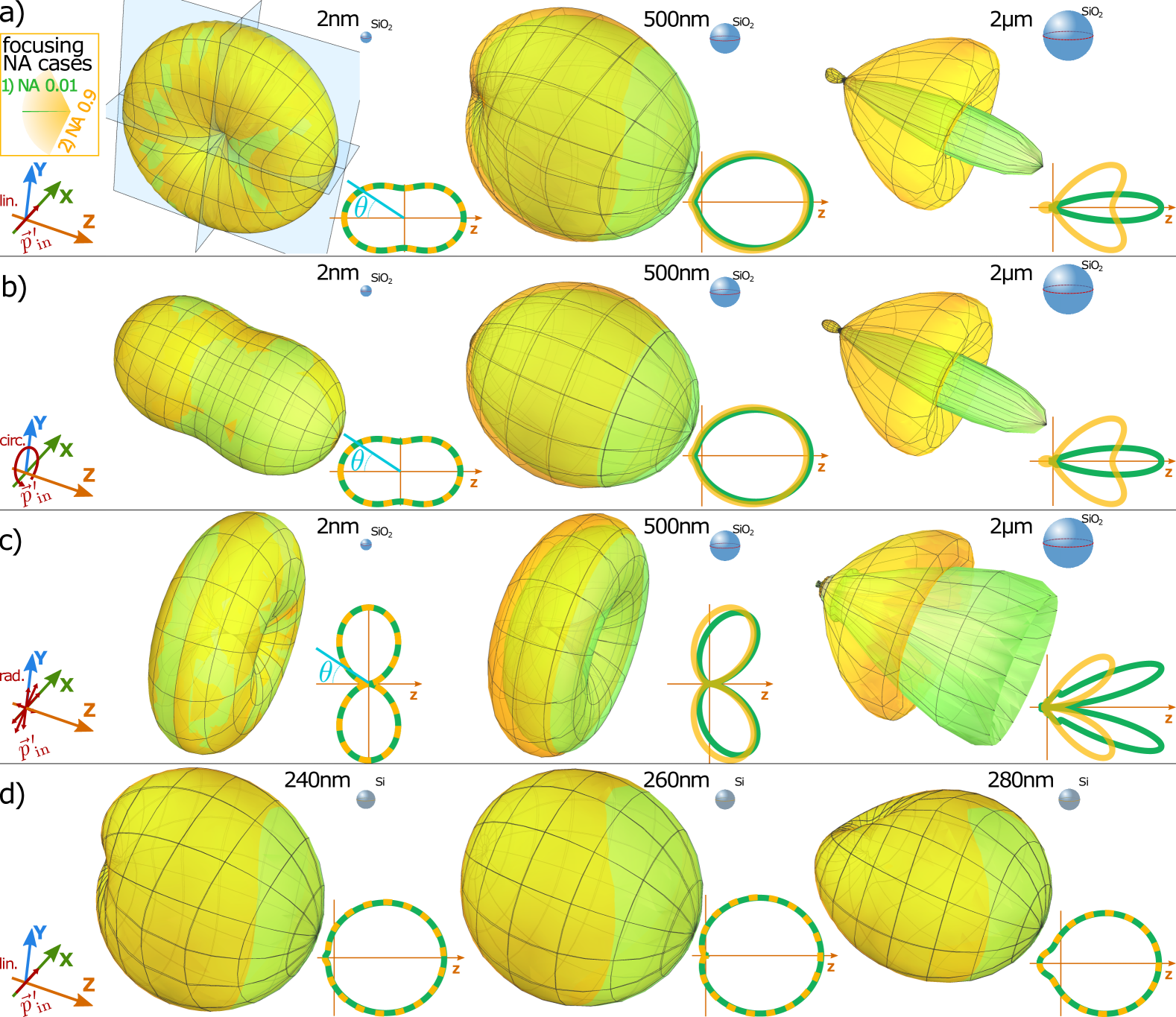
With the described routine to find the scattered field (Eq. (S3)), we evaluated the radiation patterns obtained for the silica (SiO2) nanospheres of different sizes illuminated by the incident beam with and various polarization states, see Fig. S2(a)-(c). For these figures, we choose the larger filling factor to highlight the contributions of the plane waves incident under larger angles. The selection of the silica material is driven by its wide use in optical levitation. For our calculations, we assume that the wavelength of the incident light is 1064 nm, and we chose the refractive index of silica to be . First, we were interested in the role of the focusing NA and its effect on the scattered radiation pattern. Therefore, we evaluated distributions for two contrasted NA values, and presented in Fig. S2 with green and orange hues, respectively. Second, we chose three types of polarizations of the incident light, which were discussed when presenting Eqs. (S4),(S5), namely linear, circular and radial polarizations. These cases are given in Fig. S2 in the panels (a), (b), and (c), respectively. Third, for the wavelength of the incident light of 1064 nm, we chose three different diameters of the spheres, 2nm, 500nm, and 2000nm, which are displayed in the left, middle, and right columns in panels (a), (b) and (c), correspondingly. Besides silica dielectric material, we also evaluated several patterns for silicon nanospheres, with complex refractive index , under the incidence of the linearly polarized Gaussian beam. For the three diameters (240nm, 260nm, and 280nm) in the vicinity of the size (nm) where the Kerker condition is satisfied (see Sec. V.2), we obtained radiation patterns presented in Fig. S2(d).
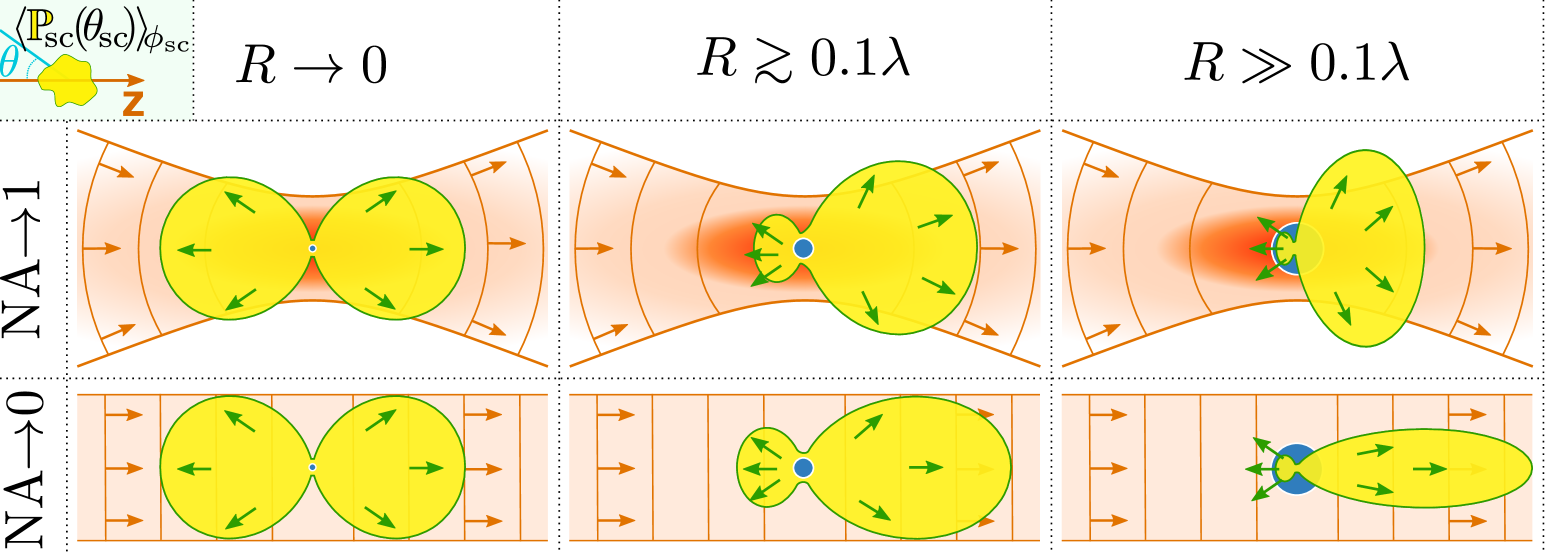
Based on these results, we can conclude that the sphere’s radius growth leads to the drastic radiation power redistribution between backward and forward directions. For the plane incident wave, the forward distribution forms an unidirectional angular lobe whose angular span decreases with further radius increase, gaining unidirectionality. Here, we confine our discussion with the general behavior, but the exceptional conditions available for will be shined further in Sec. V.2. For another variable parameter - focusing NA, we also observe its impact becoming noticeable for a larger radius. Although, even for a relatively small silica sphere with a radius of 250 nm, one can notice the tendency to suppress the forward scattered radiation () and redistribute the energy to the lateral directions x, y. The high NA leads to the transformation of the unidirectional lobe to the flattened shape. To summarize the observations, we give a schematic representation of the observed behavior in Fig. S3, to make the above qualitative observations more comprehensible.
V.2 Kerker effect
In this section, we discuss the Kerker effect (see [22, 23]), which causes the light scattering to be predominantly forward-directed, and examine the asymmetry factor that characterizes this directivity. The idea behind the Kerker effect [see, e.g., [32]] lies in control and optimization of the magnitude and phase of the complex coefficient , , discussed in Sec. V.1, in order to suppress the backward (forward) scattering light. The straightforward condition to realize the Kerker effect and suppress backward scattering (so-called first Kerker condition) is attaining the equality of complex magnitudes of the electric and magnetic dipoles, namely . This condition leads to the destructive interference between these two contributions along the negative valued axis and constructive interference along the positive valued axis, with the object placed at .
To demonstrate the role of the interference between the electric field generated by magnetic and electric sources induced in a sphere, we use the asymmetry parameter (see, e.g., Sec. 3.11 [50], Sec. 2.3 in [91], Sec. 4.5 [92]). The asymmetry parameter is the mean magnitude of weighted by the weighting function such that
| (S6) |
and represent the balance between back- and forward-scattered light. The cases and correspond to light scattered more in the direction opposite or along the z-axis, respectively. As it follows from Eq. (S6), the magnitude of as high as directivity of the scattered light and get its maximum for the case (in the coordinate system we chose, see Fig. S1). For the spherical-shaped dielectric scatterer and linear polarized incident plane wave, the asymmetry parameter can be calculated as follows:
| (S7) |
where coefficients and were presented in Sec. V.1 being introduced in Eqs.(S1), and we set as in the general computations discussed in Sec. V.1.
Evaluation of the asymmetry factor and finding its local maxima allow us to find the conditions that provide the minimal radiation pressure, that leads to lowering recoil energy and parameter . In this regard, we calculated the magnitude of asymmetry factor given in Eq. (S7) for the range of real-valued refractive index and radii [1 nm, 250 nm] assuming the wavelength of the incident light to be of . The obtained distribution presented in Fig. 2 in the main text allows us to find the radius of the scatterer for any non-absorbing materials providing significant forward scattering, and represented as highest magnitudes of the . To tackle the role of the reduction of , in the current work, we use three materials: silica (), silicon (Si), and diamond (Di). We emphasize that any high refractive material can be used for such procedure in general (see, e.g., [26]). For the given materials with refractive indexes and , we have the maxima of asymmetry factor at and . To demonstrate the important role of the radius choice, we plot the radiation pattern of the Si nanosphere near the radius of the maximum forward scattering . From Fig. S2(d), it is evident that even a slight change in the particle size affects the symmetry of the radiation pattern.
V.3 Scattering cross-section
The cross-section () of Mie particles illuminated by a linearly polarized plane wave is given by equation (see, e.g., Sec. 4.4.1 [92] and Sec. 6.1 in [90])
| (S8) |
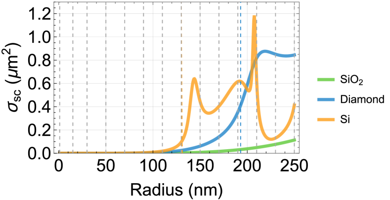
coefficients and are the same as in previous sections. Figure S4 displays as a function of radius for silica, diamond, and silicon nanospheres obtained by Eq.(S8). This equation can also approximate the results for cross-sections when Mie particles are illuminated by a weak focused beam, linearly polarized wave with small NA. Therefore, the results presented in Fig.S4 serve us as a benchmark with the reference magnitudes for low NA cases.
Since Eq.(S8) can not be used directly for the scattering processes involving high NA, and does not account for the radial polarization of the incident beam, the alternative approach to calculate the cross-section has to be used. For the low-absorbing particles considered in this work, the scattering cross-section is equivalent to the extinction cross-section and can be found via the optical theorem as
| (S9) |
However, this definition is only valid for incident beams with defined polarization states and the nonzero scattered light along the optical axes. Since the radially polarized modes have undefined polarization at their center, and since the scattering of radially polarized light by Mie particle results in a zero electric field along the optical axis (see,e.g., Fig. S2(c)), using of the Eq. S9 is impossible (see, e.g., [54]). To overcome this limitation, we calculated using numerically calculated distributions of and substituting them in the general definition of the scattering cross-section (see, e.g., Sec. 1.1 in [90], Sec. 3.4 in [92] and [54]):
| (S10) |
Here , and is intensity of the incident field at exact position of the focus , which is defined as . The electric fields for linearly and radially polarized focused beams were obtained by calculations presented in [87]. The obtained distributions of in dependence on the radius of the particle and focusing NA are presented in Fig. S5 and were plotted by spline function of the first order interpolating results obtained in the coordinates marked with dark points.
We compared the results in Fig. S5 (top row), obtained for the incident linear polarization, with those obtained for the plane incident wave given in Fig. S4. This comparison was performed across the entire set of calculated points and was consistent for the selected radii. The peaks at about 146 nm and 207 nm corresponded to silicon and are not resolved in Fig. S5 due to the grid we have chosen.
The observed agreement for linearly polarized incident beams validates the approach used with Eq. (S10). This consistency gives us confidence in applying the same method to obtain the scattering cross-section for radially polarized beams, as shown in Fig. S5 (bottom row).