Moiré Superradiance in Cavity Quantum Electrodynamics with Quantum Atom Gas

Abstract

As a novel platform for exploring exotic quantum phenomena, the moiré lattice has garnered significant interest in solid-state physics, photonics, and cold atom physics. While moiré lattices in two- and three-dimensional systems have been proposed for neutral cold atoms, the simpler one-dimensional moiré effect remains largely unexplored. We present a scheme demonstrating moiré effects in a one-dimensional cold atom-cavity coupling system, which resembles a generalized open Dicke model exhibiting superradiant phase transitions. We reveal a strong link between the phase transition critical point and the one-dimensional moiré parameter. Additionally, we derive the cavity field spectrum, connected to the dynamical structure factor, and showcase controlled atomic diffusion. This work provides a new route for testing one-dimensional moiré effects with cold atoms and open new possibility of moiré metrology.

Two-dimensional (2D) moiré lattices engineered by stacking two 2D periodic layers with a relative twisting angle have emerged as an intriguing new experimental platform in solid-state physics and optics, in which many exotic phenomena have been unraveled, including unconventional superconductivity Bistritzer and MacDonald (2011); Cao et al. (2018); Tarnopolsky et al. (2019), quantum Hall effect Dean et al. (2013), non-Abelian gauge potentials San-Jose et al. (2012), and localization Wang et al. (2020). As a powerful playground for quantum simulation Bloch et al. (2008), efforts are pushing forward towards implementing moiré lattice via trapping neutral cold atoms in 2D and three-dimensional optical lattices González-Tudela and Cirac (2019); Salamon et al. (2020a, b); Luo and Zhang (2021); Meng et al. (2023); Wang et al. (2024), which essentially focus on the moiré physics of flat band. Noteworthy while one-dimensional (1D) superlattice have already been implemented in cold atoms to demonstrate localization Roati et al. (2008); Schreiber et al. (2015), the 1D moiré effects in which moiré parameter would play a vital role in the system quantum properties remain largely unexplored. Whilst in the counterpart electronic and optical systems, the research on 1D moiré effects are burgeoning Vu and Das Sarma (2021); Talukdar et al. (2022); Yu et al. (2023); Gonçalves et al. (2024); Li et al. (2025). Question naturally arises on whether one can observe moiré effects in a 1D setup with cold atoms.

Here we propose a scheme to test such effects, specifically in a cold atom-cavity coupling system enabling superradiant phase transition. As sketched in Fig. 1, a cold atom gas composed of $N$ atoms of mass $m$ are trapped along the axis of a standing-wave optical resonator in the $x$-direction, and also illuminated by a laser incident from the cavity side. The driving laser is detuned far below the atomic transition, thus are scattered by the atoms into the cavity mode with a pump strength $\varepsilon_{p}$. The system can be mapped to the well-known Dicke model in quantum optics Baumann et al. (2010); Nagy et al. (2010); Klinder et al. (2015a). Upon driving the pump across a critical value, the interplay between cavity-mediated global interaction among atoms and cavity decay would bring the system into a steady state with diverging excitations, in which photons are collectively scattered into the cavity mode and the atoms self-organize themselves in the combined net potential of trapping and emerging intracavity standing-wave potential. A lot of studies on systems of this type have been reported, both in theory Nagy et al. (2011); Sandner et al. (2015); Maschler et al. (2007); Cosme et al. (2018); Zheng and Cooper (2018); Yin et al. (2020); Mivehvar (2024); Han et al. (2024) and experiment Landig et al. (2015); Klinder et al. (2015b); Landig et al. (2016); Landini et al. (2018); Vaidya et al. (2018).

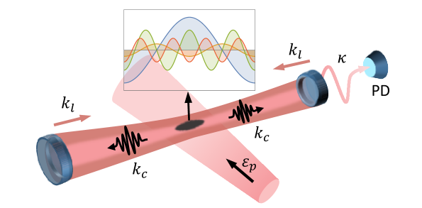
Figure 1: Schematic diagram for dissipative phase transition in a cavity-assisted moiré lattice. Atoms are trapped by a optical lattice potential $V_{l}\cos^{2}(k_{l}x)$ along the cavity axis. Atoms scatter the side pump laser $\varepsilon_{p}$ into the cavity mode $\cos(k_{c}x+\phi)$. The inset show atom self-ordering in the combined 1D moiré lattice. Cavity decay rate is $\kappa$.

To build the moiré lattice, we consider an additional one-dimensional (1D) optical lattice is applied on the atoms, the optical lattice potential $V_{l}\cos^{2}(k_{l}x)$ is chosen incommensurate to the intracavity standing-wave mode $\cos(k_{c}x+\phi)$. Then ratio $r=k_{c}/k_{l}$ defines the moiré ratio of a combined 1D bichromatic moiré lattice Vu and Das Sarma (2021). Specifically we set $r$ as the ratio of two consecutive numbers of the Fibonacci sequence, i.e., $r=f_{n+1}/f_{n}$. Fibonacci sequence is defined by the recursion relation $f_{n+1}=f_{n-1}+f_{n}$ with $f_{0}=f_{1}=1$, in the $n\rightarrow\infty$ limit $r$ approaches the golden ratio $(\sqrt{5}+1)/2$. The 1D moiré lattice is quasiperiodic with a unit cell length $L=2\pi/k_{0}$, where $k_{0}$ denotes the elementary wave number with $k_{l(c)}=f_{n(n+1)}k_{0}$. Here we introduce the lowest common numerator of $r$ as the moiré parameter $M$ ($=f_{n+1}$), in the following we illustrate with three cases of $M=1,3,5$, correspond to $n=1,3,4$ respectively. For simplicity we assume the relative phase $\phi=0$.

The dynamics of the joint atom-cavity density operator follows from the master equation Mivehvar et al. (2021); Ritsch et al. (2013)

$$\dot{\rho}=\frac{1}{i\hbar}[H,\rho]+\kappa(2a\rho a^{\dagger}-a^{\dagger}a\rho-\rho a^{\dagger}a),$$ (1)

where

$$H =H_{C}+H_{A}+H_{AC},$$

$$H_{C}/\hbar =-\delta_{c}a^{\dagger}a,$$

$$H_{A}/\hbar =\int dx\Psi^{\dagger}(x)\left[-\frac{\hbar}{2m}\partial_{x}^{2}+V_{l}\cos^{2}(k_{l}x)\right]\Psi(x),$$

$$H_{AC}/\hbar =\int dx\Psi^{\dagger}(x)\left[U_{0}a^{\dagger}a\cos^{2}(k_{c}x+\phi)\right.$$

$$\left.+\varepsilon_{p}(a+a^{\dagger})\cos(k_{c}x+\phi)\right]\Psi(x).$$ (2)

Here the cavity mode is described by an annihilation operator $a$, which subject to decay with a rate $\kappa$. $\delta_{c}$ is the cavity-pump detuning. $\Psi(x)$ is the atom bosonic field operator. $U_{0}$ stands for the light shift per intracavity photon, in the case of frequency redshift $U_{0}<0$.

The atom field can be effectively expanded with a finite number of modes

$$\Psi(x)=\sqrt{\frac{1}{L}}c_{0}+\sum_{n=1}^{n_{c}}\sqrt{\frac{2}{L}}\cos(nk_{0}x)c_{n},$$ (3)

where the $c_{0(n)}$ are bosonic annihilation operator. We have precluded the odd parity (sine) modes by considering the parity symmetry for bosons initially in a Bose-Einstein condensate. Note that collisional atom-atom interactions can be tuned small and they only play a role in shifting the single particle dispersion Baumann et al. (2010), so we neglect collisional interactions here without affecting the main physics. A cutoff $n_{c}$ is introduced due to that high energy modes are less likely to be excited. Insert (3) into (2), by evaluating the integrals within one unit cell we can obtain the Hamiltonian in a reduced subspace as

$$H/\hbar =-\delta_{c}a^{\dagger}a+\omega_{k}c^{\dagger}\mathcal{K}c+\frac{V_{l}}{4}c^{\dagger}\mathcal{M}_{2f_{n}}c$$

$$+\frac{U_{0}}{4} a^{\dagger}ac^{\dagger}(2\mathds{1}+\mathcal{M}_{2f_{n+1}})c+\frac{\varepsilon_{p}}{2}(a+a^{\dagger})c^{\dagger}\mathcal{M}_{f_{n+1}}c,$$ (4)

where $c=(c_{0},c_{1},\dots,c_{n_{c}})^{T}$, the recoil frequency $\omega_{k}=\hbar k_{0}^{2}/2m$, $\mathds{1}$ is the identity matrix, the matrices $\mathcal{K}$, $\mathcal{M}_{f_{n}}$ are given in sm . Since in real experiment cavity mode is usually fixed, then in the following we scale the energy with $\omega_{r}=\hbar k_{c}^{2}/2m=M^{2}\omega_{k}$. That is to say, moiré parameter is manipulated by $k_{l}$. Hamiltonian (4) typically represents an extended Dicke model, in which the quantum light field is effectively coupled to multilevel transitions of many atoms. In addition to scattering within the cavity, the externally applied lattice allows for momentum transfers among atoms, giving rise to moiré effects in atom self-ordering and superradiant phase transition as will be illustrated below.

Mean-field solution and excitations.— In the $N\rightarrow\infty$ mean-field limit, the operators $a$, $c_{0(n)}$ split into

$$a=\sqrt{N}\alpha+\delta a,~c_{0(n)}=e^{-i\mu t}\left[\sqrt{N}\psi_{0(n)}+\delta c_{0(n)}\right],$$ (5)

where $\alpha$, $\psi_{0(n)}$ are scaled steady state expectations with $\delta a$, $\delta c_{0(n)}$ characterize the corresponding quantum fluctuations, $\mu$ is the chemical potential. By solving stationary equations sm , the cavity field amplitude $|\alpha|$ are plotted in Fig. 2 versus the scaled pumping strength $\eta=\sqrt{N}\varepsilon_{p}$.

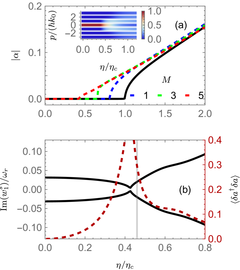
Figure 2: (a) Scaled mean-field value $|\alpha|$ versus scaled pumping strength $\eta$ for different $M$. The black solid line is the case without the external optical lattice. The inset showcase steady state momentum distribution for $M=5$. (b) The eigenvalues imaginary parts of the lowest atom polariton excitation and incoherent cavity excitation versus $\eta$ for $M=5$. The vertical grey line indicate the analytical phase transition point sm . The steady states and excitations are calculated for $V_{l}=-1$, $NU_{0}=-80$, $\Delta_{c}=-100$ and $\kappa=20$.

Without the external optical lattice potential, the present system exactly resemble the open Dicke model Nagy et al. (2011). In the thermodynamical limit the mean-field solutions would predict a critical pumping strength $\eta_{c}=\sqrt{-(\Delta_{c}^{2}+\kappa^{2})\omega_{r}/2\Delta_{c}}$ with effective detuning $\Delta_{c}=\delta_{c}-NU_{0}/2$, which separates the normal phase $\left\{\alpha=0,\psi_{0}=(1,0,0,\dots)^{T}\right\}$ from the superradiant phase with a finite $\alpha$. In Fig. 2(a) this case is indicated by a black solid line. With the increase of moiré parameter $M$, one can see that the corresponding critical pumping gradually decreases. Upon the onset of superradiant phase transition, in the steady state atoms disperse from the homogeneous state into the modulated states, as illustrated in the inset of Fig. 2(a) for $M=5$.

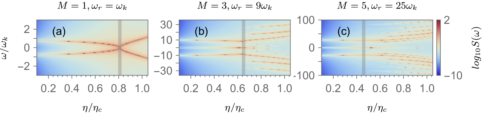
Figure 3: The logarithm of the cavity field spectrum $S(\omega)$ as a function of $\omega$ and relative pumping $\eta$. From left to right: (a) $M=1$, (b) $M=3$, (c) $M=5$. The vertical gray bar indicate the critical pumping strength at which phase transition takes place for each cases. Below threshold two pairs of sideband peaks are visible, corresponding to frequencies of two types of quasi-particle excitations as specified in the main text. Upon the onset of superradiant phase transition, more peaks appear and they are intimately related to the moiré parameter $M$.

The relation between the critical pumping strength and the moiré parameter $M$ can be understood via a study on the excitation properties sm : The moiré lattice provides an additional scattering channel of atoms in the $\cos(2k_{l}x)$ mode are scattered by the pump field into the cavity photon, resulting in atomic polariton excitations with eigenfrequency $w_{j=2f_{n}-f_{n+1}}$ which is much less than that in the usual scattering channel involving atoms in the homogeneous state. Increasing $M$ effectively equals enlargement of the lattice constant, which will decrease the energy gap and thus facilitating superradiant phase transition. In Fig. 2(b) we mark the analytic critical value for $M=5$ as the vertical line, which approximately coincide with the point at which the imaginary parts of the lowest atom polariton excitation frequency (black solid lines) reach zero. Incoherent cavity field excitation $\left\langle\delta a^{\dagger}\delta a\right\rangle$ (red-dashed line) also becomes divergent upon the onset of phase transition.

Cavity field spectrum.— The onset of phase transition can be indicated by the dynamic structure factor, which is the Fourier transform of the intracavity field correlator $S(\omega)\equiv\mathcal{F}\left(\left\langle a^{\dagger}\left(t_{s}+t\right)a\left(t_{s}\right)\right\rangle\right)$ ($t_{s}$ is the time for the system to reach steady state) and thus can be probed in experiment Landig et al. (2015); Agarwal (2006). We calculate $S(\omega)$ sm with the results presented in Fig. 3.

To map the dynamical structure factor, in the spectra plotted we have dropped the coherent part of $\omega=0$ Landig et al. (2015), which would become prominent upon the onset of superradiant phase transition as photons are collectively scattered into the cavity mode. The spectra are almost symmetric with respect to $\omega=0$ and their peaks come in pairs. Peaks of cavity spectrum actually reflect frequencies of atomic polariton mode excitation consisting of photonic and atomic parts sm . In the regime far below the threshold, the spectra peaks are located at $\omega\simeq\pm\omega_{r}$ and $\pm\omega_{k}=\pm\hbar(2k_{l}-k_{c})^{2}/2m$, reflecting that the cavity photons are scattered from the atoms in the homogeneous mode and those in the mode of $\cos(2k_{l}x)$, respectively. With the increase of pumping strength, the peaks in both pairs gradually move toward each other, the $\pm\omega_{k}$ peaks even merge at the critical point. This behavior is because the photonic components are becoming larger in the atomic polariton modes sm , and upon the phase transition, the lowest atomic polariton excitation frequency approaches zero, as also indicated in Fig. 2(b). Beyond the critical point, more pairs of peaks appear with the increase of the moiré parameter $M$, and the peaks of a pair tend to repel from each other when the pumping is continuously enhanced. The phenomena root in the fact that more atomic polariton modes are excited and their energies increase as well. The intracavity field spectra (dynamical structure factor) predicted here can serve as evidence of moiré effects on the superradiant phase transition.

Truncated Wigner approximation (TWA) simulation.— In order to verify whether the phenomena predicted above in the thermodynamical limit can really take place in a finite quantum system, here we simulate the dynamics in the open system depicted by the master equation (1). Due to the in principle unconstrained Hilbert space dimension of the cavity field in a generalized Dicke model and its global coupling to all the atomic modes, a full quantum simulation hiring Monte-Carlo wavefunction (quantum jump) algorithm is usually limited to small system size Sandner et al. (2015); Halati et al. (2020). We adopt TWA to study the dynamics sm . The TWA method Sinatra et al. (2002); Blakie et al. (2008); Polkovnikov (2010); Schachenmayer et al. (2015) have found qualitative agreements with experimental results in a series of atom-cavity setup of time crystal experiments Keßler et al. (2021); Kongkhambut et al. (2021); Skulte et al. (2023).

As shown in Fig. 4(b), in every run of TWA simulation we propagate an initial state of $N=1000$ atoms in the homogeneous mode $\psi_{0}$ while the other atomic modes and the cavity field are left empty, by ramping the cavity pumping up to a desired value $\eta$ and holding it there until a steady state is reached. Compared with mean-field results, the TWA calculation indicate that onset of superradiant phase transition will apparently takes place at a smaller critical pumping $\eta$, as illustrated in Fig. 4(a). This suggests that quantum fluctuations will lower the critical value for the phase transition to take place. Apart from that, the dependence of superradiant phase transition on the moiré parameter is verified. In the right panel of Fig. 4(a), for $\eta=0$ steady state population in homogeneous mode $\psi_{0}$ becomes smaller with increasing $M$. This behavior is because the external optical lattice scatter the $\psi_{0}$ atoms into $\psi_{2k_{l}}$, whose scaled kinetic energy $4k_{l}^{2}/k_{c}^{2}=4/r^{2}$ decreases when $M$ becomes larger. The larger seed population of $\psi_{2k_{l}}$ in turn triggers dynamical instability of the normal phase at a smaller pumping strength $\eta$ sm .

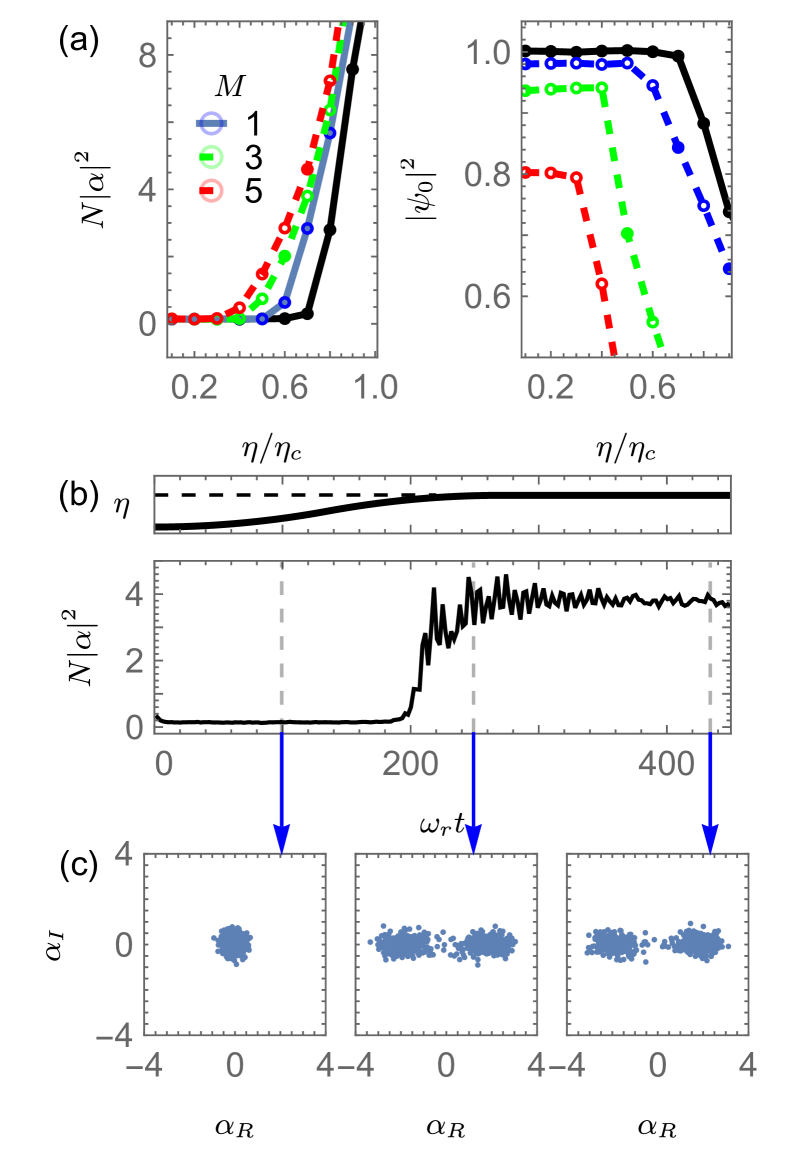
Figure 4: TWA simulation results with $N=1000$ obtained from sample of $500$ trajectory runs. (a) Steady state population in cavity mode (left panel) and homogeneous atomic mode $\psi_{0}$ (right panel) versus pumping strength $\eta$. The black solid line is the case without the external optical lattice. (b) Cavity field population dynamics at $M=3$ along with $\eta$ ramps to the value of $0.6\eta_{c}$. (c) Wigner distributions of cavity light field at the instant marked by the black dashed line in (b). The parameters are the same as those in Fig. 2, noticeably that TWA however predicts the superradiant phase transition to occur at lower $\eta$.

Although the presented TWA results already showcase the properties of phase transition, it is argued that finite system size will smoothen the abrupt change upon phase transitions in the thermodynamical limit Sandner et al. (2015), rendering that neither $|\alpha|^{2}$ nor $|\psi_{0}|^{2}$ a good phase transition indicator. Phase transitions are accompanied with spontaneous symmetry breaking. In the absence of the external optical lattice, with the occurrence of superradiance and the formation of intracavity optical lattice, atoms can spontaneously choose even or odd lattice sites to reside, which entangle with cavity field of opposite amplitudes and result in a macroscopic superposition state of $|\text{even}\rangle\otimes|\alpha\rangle+|\text{odd}\rangle\otimes|-\alpha\rangle$ Domokos and Ritsch (2002); Maschler et al. (2007). Similar processes take place for the present moiré lattice. For the dynamics of above threshold pumping in the $M=3$ case studied in Fig. 4(b), we project the cavity field sample of $500$ trajectories at three different times onto Fig. 4(c), which unravel its Wigner distribution. The cavity field evolves from vacuum noise (left panel), then being stretched and splitted (middle panel), and finally forms a Schrödinger cat state with opposite amplitudes (right panel). The associated atom steady states would be that atoms located at a few different sites of the combined moiré lattice. Due to the inherent symmetry of steady state, $\langle a\rangle$ or equivalently $\langle c^{\dagger}\mathcal{M}_{f_{n+1}}c\rangle$ would give the value $0$. To break the symmetry, one can project the system state with respect to one cavity state maximizing the Wigner distribution and resolve the corresponding order parameters Sandner et al. (2015); Ostermann et al. (2020).

Atomic diffusion.— Considering the long time for the system to reach steady state versus limited lifetime of cold atoms, on the atomic part it would be more practicable to observe moiré effects through their diffusion. The dependence of superradiant phase transition on the moiré parameter provides an extra control knob on atom diffusion. This can be implemented by loading atoms into the cavity and observing their transport along the moiré lattice. We study the atom diffusion by taking the initial atomic wavefunction to be a Gaussian wavepacket with width $w$, while the cavity is in vacuum. Then the pump is tuned on and the wavepacket width is estimated with $w=\sqrt{\left\langle\left(\Delta x\right)^{2}\right\rangle}$ sm .

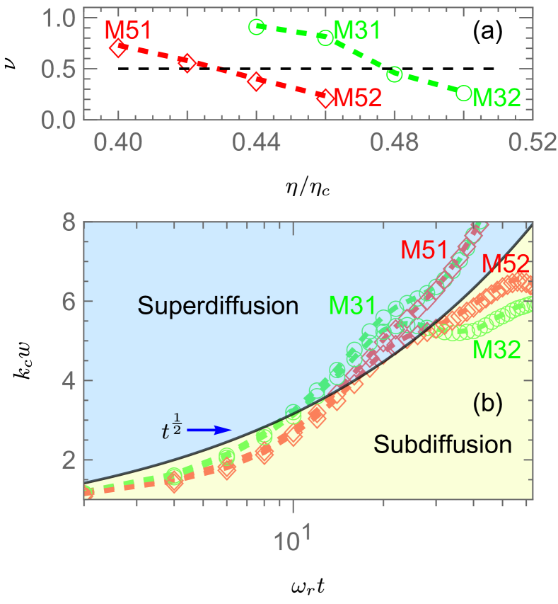
Figure 5: (a) Time scaling $\nu$ of atomic diffusion versus pumping strength $\eta$ for $M=3$ (green-dashed line) and $M=5$ (red-dashed line). The horizontal black-dashed line of $\nu=1/2$ indicates the critical scaling. (b) Atomic diffusion dynamics simulated for M31 ($M=3,\eta=0.46\eta_{c}$), M32 ($M=3,\eta=0.5\eta_{c}$), M51 ($M=5,\eta=0.4\eta_{c}$) and M52 ($M=5,\eta=0.46\eta_{c}$), which were also indicated in (a). The black line indicates the normal diffusion of $\nu=1/2$ that separates superdiffusion ($\nu>1/2$) and subdiffusion ($\nu<1/2$) regions. The parameters are the same as before.

The time evolution of $w(t)$ can be parametrized as $w(t)\sim t^{\nu}$ Larcher et al. (2009); Hiramoto and Abe (1988); Zhou et al. (2013). $\nu=1$ correspond to ballistic expansion. Under the combined effects of moiré lattice and cavity field quantum fluctuation, atoms would exhibit anomalous diffusion. We extract the time scaling $\nu$ from the atomic diffusion dynamics and present the results in Fig. 5(a). As expected, the value of $\nu$ decreases when pumping $\eta$ becomes stronger, signaling the system transfers from the regime of superdiffusion to that of subdiffusion. The boundary of the two regimes is identified with $\nu=\frac{1}{2}$. The superdiffusion to subdiffusion transfer is accompanied with the onset of superradiant phase transition and buildup of moiré lattice. This observation suggests a relation between atom diffusion and moiré pattern. As shown in Fig. 5(a), the scaling behavior indicate that superdiffusion to subdiffusion transition takes place at a smaller $\eta$ for the $M=5$ case (red-dashed line) as compared with that of $M=3$ (green-dashed line). This is consistent with our above analysis on the relation between moiré parameter and superradiant phase transition. Specifically, we examine two cases of M31 and M52, as indicated in Fig. 5(a), they subject to identical pumping of $\eta=0.46\eta_{c}$ however different $M$. M31 displays superdiffusion while M52 behaves subdiffusion, as demonstrated in Fig. 5(b). More detailed discussions on diffusion are given in the supplemental material sm .

Discussion and outlook.— We have studied moiré effects on superradiant phase transition in a cold atom-cavity coupling system. This system resembles a generalized open Dicke model. The prominent role of moiré parameter in superradiant phase transition is explicitly explored. Implementing an optical lattice for ⁸⁷Rb Bose-Einstein condensate inside a high-finesse optical cavity is feasible with existing technology Klinder et al. (2015b); Landig et al. (2016); Vaidya et al. (2018).

To observe the moiré effects, one can either utilize the optical means of cavity transmission spectrum or monitor atom diffusion. We have demonstrated that atom diffusion is controlled by the moiré parameter, and provides an ideal experimental observable to reveal the effects produced by the moiré pattern. In future work it will be interesting to look into the combined effects of moiré geometry and quantum fluctuations on superfluidity, in which one will need to estimate physical quantities such as superfluid fraction (weight) Carusotto and Castin (2011); Sidorenkov et al. (2013); Ho and Zhou (2010); John et al. (2011); Edge and Cooper (2011); Krinner et al. (2013); Biagioni et al. (2024). Besides that, one can also expect to observe moiré effects in fermionic superradiance Keeling et al. (2014); Piazza and Strack (2014); Chen et al. (2014); Zhang et al. (2021); Pan (2022); Wu et al. and many body localization Huse et al. (2014); Jie et al. (2022); Mondaini and Cai (2017); Chanda and Zakrzewski (2022). As criticality can serve as a valuable source for quantum metrology Zanardi et al. (2008); Macieszczak et al. (2016); Garbe et al. (2020); Chu et al. (2021); Ding et al. (2022); Ilias et al. (2022); Garbe et al. (2022); Gietka et al. (2022); Aybar et al. (2022); Guan and Lewis-Swan (2021); Zhou et al. (2023); Wang and Marzolino (2024) and intimate relation between moiré parameter and superradiant phase transition have been revealed here, enhanced estimation on the moiré parameter would enrich the physics of moiré metrology Kafri and Glatt (1990); Post and Han (2008); Halbertal et al. (2021).

Supplementary Materials for
blue Moiré Superradiance in Cavity Quantum Electrodynamics with Quantum Atom Gas
This PDF file includes:
Supplementary Notes I-VI
I. Matrix definition
II. Stationary equation solution
III. Excitations
IV. Cavity spectrum
V. Truncated Wigner methods
VI. Atom diffusion dynamics
Fig. S1
Fig. S2

I matrix definition

The matrices $\mathcal{K}$, $\mathcal{M}_{f_{n}}$ denote the kinetic energy term and the terms propotional to $\cos(f_{n}k_{0}x)$ in the Hamiltonian, which are defined as

$$\mathcal{K}=\left(\begin{array}[c]{ccccccc}0^{2}&&&&&&\\ &1^{2}&&&&&\\ &&2^{2}&&&&\\ &&&\ddots&&&\\ &&&&\ddots&&\\ &&&&&(n_{c}-1)^{2}&\\ &&&&&&n_{c}^{2}\\ &&&&&&\end{array}\right),~\mathcal{M}_{f_{n}}=\left(\begin{array}[]{ccccccc}&&&&\sqrt{2}&&\\ &&&1&&1&\\ &&\iddots&&&&\ddots\\ &1&&&&&\\ \sqrt{2}&&&&&&\\ &1&&&&&\\ &&\ddots&&&&\end{array}\right).$$ (S1)

In $\mathcal{M}_{f_{n}}$ modes $\cos(j(k)k_{0}x)$ with $j\pm k=f_{n}$ are coupled, giving a nonzero element.

II solve stationary equation

The Heisenberg-Langevin equations for the field amplitude $a$, $c_{0(n)}$ read

$$\dot{a} =\left[i\left(\delta_{c}-\frac{U_{0}}{4}c^{\dagger}(2\mathds{1}+\mathcal{M}_{2f_{n+1}})c\right)-\kappa\right]a-i\frac{\varepsilon_{p}}{2}c^{\dagger}\mathcal{M}_{f_{n+1}}c+a_{in},$$

$$\dot{c} =-i\left[\omega_{k}\mathcal{K}+\frac{V_{l}}{4}\mathcal{M}_{2f_{n}}+\frac{U_{0}}{4}a^{\dagger}a(2\mathds{1}+\mathcal{M}_{2f_{n+1}})+\frac{\varepsilon_{p}}{2}(a+a^{\dagger})\mathcal{M}_{f_{n+1}}\right]c,$$ (S2)

where the Gaussian noise operator $a_{in}$ has zero mean $\langle a_{in}(t)\rangle=0$ and nonvanishing correlation $\langle a_{in}(t)a_{in}^{\dagger}(t^{\prime})\rangle=\kappa\delta(t-t^{\prime})$. Inserting $a=\sqrt{N}\alpha+\delta a,~c_{0(n)}=e^{-i\mu t}\left[\sqrt{N}\psi_{0(n)}+\delta c_{0(n)}\right]$ into Eqs. (S2), the corresponding mean-field stationary equations can be derived as

$$[\Delta(\psi)-i\kappa]\alpha+\frac{\eta}{2}\psi^{T}\mathcal{M}_{f_{n+1}}\psi=0,~\mathcal{C}(\alpha)\psi=\mu\psi,$$ (S3)

where $\psi=(\psi_{0},\psi_{1},\dots,\psi_{n_{c}})^{T}$, $u=\frac{NU_{0}}{4}$, $\Delta_{c}=\delta_{c}-2u$, $\eta=\sqrt{N}\varepsilon_{p}$ and

$$\Delta(\psi)=-\Delta_{c}+u\psi^{T}\mathcal{M}_{2f_{n+1}}\psi,~\mathcal{C}(\alpha)=\omega_{k}\mathcal{K}+\frac{V_{l}}{4}\mathcal{M}_{2f_{n}}+u|\alpha|^{2}(2\mathds{1}+\mathcal{M}_{2f_{n+1}})+\eta\operatorname{Re}(\alpha)\mathcal{M}_{f_{n+1}}.$$ (S4)

Eqs. (S3) can be solved in a self-consistent manner. Start from an initial guess $\alpha$, diagonalize $\mathcal{C}(\alpha)$ to find out the $\psi$ corresponding to minimum $\mu$. Use this $\psi$ to derive a new $\alpha$, then repeat the above process until convergence is reached.

III excitations

Hiring linear pertubation theory, use the steady-state solutions $\left\{\alpha,\psi\right\}$ obtained from Section II, we first perform an orthogonal tranformation

$$\delta b_{j}=\mathcal{O}^{T}\delta c_{j},$$ (S5)

with $\delta b\left(c\right)_{j}=\left(\delta b\left(c\right)_{0},\delta b\left(c\right)_{1},\dots,\delta b\left(c\right)_{n_{c}}\right)^{T}$, and $\mathcal{O}$ is a matrix whose $j$-th column contains the $j$-th eigenvector of $\mathcal{C}(\alpha)$ with the corresponding eigenvalue $w_{j}$. The equations for excitations $\left\{\delta a,\delta b_{j}\right\}$ then read

$$\frac{d}{dt}\delta a =\left[-i\Delta\left(\psi\right)-\kappa\right]\delta a-i\sum_{j}\left(\frac{\eta}{2}g_{j}^{1}+u\alpha g_{j}^{2}\right)\left(\delta b_{j}+\delta b_{j}^{\dagger}\right)+a_{in},$$

$$\frac{d}{dt}\delta b_{j} =-i\left(w_{j}-\mu\right)\delta b_{j}-i\left[\frac{\eta}{2}g_{j}^{1}\left(\delta a+\delta a^{\dagger}\right)+ug_{j}^{2}\left(\alpha^{\ast}\delta a+\alpha\delta a^{\dagger}\right)\right],$$ (S6)

where $g_{j}^{1}=\mathcal{O}^{T}\mathcal{M}_{f_{n+1}}\psi$ and $g_{j}^{2}=\mathcal{O}^{T}(2\mathds{1}+\mathcal{M}_{2f_{n+1}})\psi$. Since the quadrature $\frac{1}{2}\left(\delta b_{0}+\delta b_{0}^{\dagger}\right)$ is a constant of motion and the condensate phase fluctuation $\frac{1}{2i\sqrt{N}}\left(\delta b_{0}-\delta b_{0}^{\dagger}\right)$ would not take significant effect in the thermodynamic limit, we then neglect the fluctuation $\delta b_{0}$, deduce the Langevin equations for the operator vector $\mathcal{V}=\left\{\delta a,\delta a^{\dagger},\delta b_{1},\delta b_{1}^{\dagger},\dots,\delta b_{n_{c}},\delta b_{n_{c}}^{\dagger}\right\}^{T}$ as

$$\frac{d}{dt}\mathcal{V}=\mathcal{M}_{e}\mathcal{V}+\xi,$$ (S7)

with the elementary excitation matrix

$$\mathcal{M}_{e}=\left(\begin{array}[c]{ccccc}-i\Delta-\kappa&0&-i\left(\frac{\eta}{2}g_{1}^{1}+u\alpha g_{1}^{2}\right)&-i\left(\frac{\eta}{2}g_{1}^{1}+u\alpha g_{1}^{2}\right)&\cdots\\ 0&i\Delta-\kappa&i\left(\frac{\eta}{2}g_{1}^{1}+u\alpha^{\ast}g_{1}^{2}\right)&i\left(\frac{\eta}{2}g_{1}^{1}+u\alpha^{\ast}g_{1}^{2}\right)&\cdots\\ -i\left(\frac{\eta}{2}g_{1}^{1}+u\alpha^{\ast}g_{1}^{2}\right)&-i\left(\frac{\eta}{2}g_{1}^{1}+u\alpha g_{1}^{2}\right)&-i\left(w_{1}-\mu\right)&0&0\\ i\left(\frac{\eta}{2}g_{1}^{1}+u\alpha^{\ast}g_{1}^{2}\right)&i\left(\frac{\eta}{2}g_{1}^{1}+u\alpha g_{1}^{2}\right)&0&i\left(w_{1}-\mu\right)&0\\ \vdots&\vdots&0&0&\ddots\end{array}\right),$$ (S8)

and $\xi=\left(a_{in},a_{in}^{\dagger},0,0,\dots\right)^{T}$. A phase transition occurs if $\mathcal{M}_{e}$ inherits a zero energy eigenstate. We numerically diagonalize $\mathcal{M}_{e}$ to obtain a pair of lowest atom polariton excitations, with whose value approach $0$ we determine the phase transition critical point, as shown in Fig. 2(b) of the main text.

In the normal phase $\alpha=0$, for small $V_{l}$ one can expect that the steady-state $\psi$ have most population in the homogeneous mode and a small excitation in the mode of $\cos(2k_{l}x)$, in the meanwhile the transformation matrix $\mathcal{O}$ is essentially identity. Then one can roughly only account $j=f_{n+1}$ and $2f_{n}-f_{n+1}$ in $g_{j}^{1}$. Physically they correspond to the process in which the atoms in the homogeneous mode and those in the mode of $\cos(2k_{l}x)$ are scattered by the cavity photon, respectively. In this case we can consider the following two block matrix

$$\mathcal{M}_{ej}=\left(\begin{array}[c]{cccc}-i\Delta-\kappa&0&-i\frac{\eta}{2}g_{j}^{1}&-i\frac{\eta}{2}g_{j}^{1}\\ 0&i\Delta-\kappa&i\frac{\eta}{2}g_{j}^{1}&i\frac{\eta}{2}g_{j}^{1}\\ -i\frac{\eta}{2}g_{j}^{1}&-i\frac{\eta}{2}g_{j}^{1}&-i\left(w_{j}-\mu\right)&0\\ i\frac{\eta}{2}g_{j}^{1}&i\frac{\eta}{2}g_{j}^{1}&0&i\left(w_{j}-\mu\right)\end{array}\right),$$ (S9)

where $j=f_{n+1}$ or $2f_{n}-f_{n+1}$. $\mathcal{M}_{ej}$ can be diagonalized and give

$$\left(\begin{array}[c]{cccc}-i\Delta-\kappa&0&0&0\\ 0&i\Delta-\kappa&0&0\\ 0&0&-iw_{j}^{s}&0\\ 0&0&0&iw_{j}^{s}\end{array}\right)$$ (S10)

with $w_{j}^{s}\simeq\left(w_{j}-\mu\right)\sqrt{1-\left(\frac{\eta}{\eta_{c}}\right)^{2}}$ under $|(w_{j}-\mu)/\Delta|<<1$, which indicate a critical pumping strength of $\left(\eta_{c}g_{j}^{1}\right)^{2}=\frac{\kappa^{2}+\Delta^{2}}{\Delta}\left(w_{j}-\mu\right)$. Beyond $\eta_{c}$ the quasiparticle eigenfrequency $w_{j}^{s}$ would become complex and trigger instability of the normal phase. For the Fibonacci sequence of $\left(f_{n},f_{n+1}\right)=\left\{\left(2,3\right),\left(3,5\right)\right\}$ considered in the main text the quasiparticle mode of $j=2f_{n}-f_{n+1}=1$ will have a smaller energy gap $w_{j}-\mu$ than that of $j=f_{n+1}$, resulting in a smaller $\eta_{c}$. This is the key mechanism underlying a moiré lattice can stimulate the occurrence of phase transition. In the absence of $V_{l}$, we have $g_{1}^{1}=\sqrt{2}$, $w_{1}-\mu=\omega_{r}$ and $\Delta(\psi)=-\Delta_{c}$, resulting in a critical pumping $\sqrt{-(\Delta_{c}^{2}+\kappa^{2})\omega_{r}/2\Delta_{c}}$, which recover that of the open Dicke model.

With the increase of the moiré parameter $M$, the value of $w_{j}-\mu$ will decrease as can be seen from the expression of $\mathcal{C}(\alpha)$ (S4) since $\omega_{k}=\omega_{r}/M^{2}$, rendering that $\eta_{c}$ also decreases. Physically this can be understood as an effective enlargement of the lattice constant, which will decrease the energy gap and thus facilitating phase transition.

IV cavity spectrum

The cavity field spectrum is defined as $S\left(\omega\right)=\mathcal{F}\left(\left\langle a^{\dagger}\left(t_{s}+t\right)a\left(t_{s}\right)\right\rangle\right)$, where $\mathcal{F}\left(\cdot\right)$ indicate Fourier transform with respect to $t$, $t_{s}$ is a time long enough for the system reach stationary state. Since $\left\langle a^{\dagger}\left(t_{s}+t\right)a\left(t_{s}\right)\right\rangle=N\left|\alpha\right|^{2}+\left\langle\delta a^{\dagger}\left(t_{s}+t\right)\delta a\left(t_{s}\right)\right\rangle$, then we have

$$S\left(\omega\right) =2\pi N\left|\alpha\right|^{2}\delta\left(\omega\right)+\int dte^{-i\omega t}\left\langle\delta a^{\dagger}\left(t_{s}+t\right)\delta a\left(t_{s}\right)\right\rangle$$

$$=2\pi N\left|\alpha\right|^{2}\delta\left(\omega\right)+\left\langle\delta a^{\dagger}\left(\omega\right)\delta a\left(\omega^{\prime}\right)\right\rangle,$$ (S11)

where $\delta a\left(\omega\right)$ represent the Fourier transform of $\delta a\left(t\right)$.

We left multiply $\mathcal{O}^{l}$ on both sides of Eq. (S7), where the rows of $\mathcal{O}^{l}$ contain the left eigenvectors of the complex matrix $\mathcal{M}_{e}$, from which one can have

$$\frac{d}{dt}\mathcal{V}_{l}=\mathcal{WV}_{l}+\xi_{l},$$ (S12)

where $\mathcal{V}_{l}=\mathcal{O}^{l}\mathcal{V}=\left\{\delta d,\delta d^{\dagger},\delta e_{1},\delta e_{1}^{\dagger},\dots,\delta e_{n_{c}},\delta e_{n_{c}}^{\dagger}\right\}^{T}$, $\mathcal{W}$ is a diagonal matrix with the diagonal elements $\left\{-i\Delta-\kappa,i\Delta-\kappa,-iw_{1}^{s},iw_{1}^{s},\dots,-iw_{n_{c}}^{s},iw_{n_{c}}^{s}\right\}^{T}$, and $\xi_{l}^{j}=\mathcal{O}_{j,1}^{l}a_{in}+\mathcal{O}_{j,2}^{l}a_{in}^{\dagger}$. Introduce Fourier transforms to the quantum Langevin equations (S12) with

$$\mathcal{O}\left(\omega\right)=\frac{1}{\sqrt{2\pi}}\int_{-\infty}^{\infty}e^{i\omega t}\mathcal{O}\left(t\right)dt,\mathcal{O}^{\dagger}\left(-\omega\right)=\frac{1}{\sqrt{2\pi}}\int_{-\infty}^{\infty}e^{i\omega t}\mathcal{O}^{\dagger}\left(t\right)dt,$$ (S13)

we can deduce $\mathcal{\tilde{V}}_{l}\left(\omega\right)=\left\{\delta d\left(\omega\right),\delta d^{\dagger}\left(-\omega\right),\delta e_{1}\left(\omega\right),\delta e_{1}^{\dagger}\left(-\omega\right),\dots,\delta e_{n_{c}}\left(\omega\right),\delta e_{n_{c}}^{\dagger}\left(-\omega\right)\right\}^{T}$, with

$$\delta d\left(\omega\right) =\frac{\tilde{\xi}_{l}^{1}}{-i\left(\omega-\Delta\right)+\kappa},\delta d^{\dagger}\left(-\omega\right)=\frac{\tilde{\xi}_{l}^{2}}{-i\left(\omega+\Delta\right)+\kappa},$$

$$\delta e_{j}\left(\omega\right) =\frac{\tilde{\xi}_{l}^{j+2}}{-i\left(\omega-w_{j}^{s}\right)+\gamma},\delta e_{j}^{\dagger}\left(-\omega\right)=\frac{\tilde{\xi}_{l}^{j+3}}{-i\left(\omega+w_{j}^{s}\right)+\gamma},$$ (S14)

where $\tilde{\xi}_{l}^{j}=\mathcal{O}_{j,1}^{l}a_{in}\left(\omega\right)+\mathcal{O}_{j,2}^{l}a_{in}^{\dagger}\left(-\omega\right)$, we have phenomenologically introduced a decay rate $\gamma$ for the atomic polariton modes.

We then perform a reverse transform $\mathcal{O}^{r}\mathcal{\tilde{V}}_{l}\left(\omega\right)$ with the columns of $\mathcal{O}^{r}$ contain the right eigenvectors of $\mathcal{M}_{e}$, from which we can have

$$\delta a\left(\omega\right)=\mathcal{O}_{11}^{r}\delta d\left(\omega\right)+\mathcal{O}_{12}^{r}\delta d^{\dagger}\left(-\omega\right)+\sum_{j=1}^{n_{c}}\left[\mathcal{O}_{1,j+2}^{r}\delta e_{j}\left(\omega\right)+\mathcal{O}_{1,j+3}^{r}\delta e_{j}^{\dagger}\left(-\omega\right)\right].$$ (S15)

Combining eq. (S14) and (S15), we can have

$$\left\langle\delta a^{\dagger}\left(\omega\right)\delta a\left(\omega^{\prime}\right)\right\rangle =\left|\mathcal{O}_{11}^{r}\right|^{2}\left\langle\delta d^{\dagger}\left(\omega\right)\delta d\left(\omega^{\prime}\right)\right\rangle+\left|\mathcal{O}_{12}^{r}\right|^{2}\left\langle\delta d\left(-\omega\right)\delta d^{\dagger}\left(-\omega^{\prime}\right)\right\rangle$$

$$+\sum_{j=1}^{n_{c}}\left[\left|\mathcal{O}_{1,j+2}^{r}\right|^{2}\left\langle\delta e_{j}^{\dagger}\left(\omega\right)\delta e_{j}\left(\omega^{\prime}\right)\right\rangle+\left|\mathcal{O}_{1,j+3}^{r}\right|^{2}\left\langle\delta e_{j}\left(-\omega\right)\delta e_{j}^{\dagger}\left(-\omega^{\prime}\right)\right\rangle\right]$$

$$\simeq\sum_{j=1}^{n_{c}}\left[\frac{\kappa\delta\left(\omega-\omega^{\prime}\right)}{\left|-i\left(\omega-w_{j}^{s}\right)+\gamma\right|^{2}}\left|\mathcal{O}_{j+2,2}^{l}\mathcal{O}_{1,j+2}^{r}\right|^{2}+\frac{\kappa\delta\left(\omega-\omega^{\prime}\right)}{\left|-i\left(\omega+w_{j}^{s}\right)+\gamma\right|^{2}}\left|\mathcal{O}_{j+3,2}^{l}\mathcal{O}_{1,j+3}^{r}\right|^{2}\right],$$ (S16)

where we have assumed that the photonic polariton mode population $\left\langle\delta d^{\dagger}\left(\omega\right)\delta d\left(\omega^{\prime}\right)\right\rangle$ is vanishingly small in the case of large $\Delta_{c}$ ($\Delta$).

V truncated Wigner methods

We adopt the truncated Wigner approximation (TWA) to study the dynamics and obtain the results presented in Fig. 4 of the main text. In an open system, we first apply Wigner-Weyl transform on both sides of the master equation (1) to obtain the evolution equation for the Wigner function $\mathcal{W}$, in which we neglect third-order derivatives under TWA. The resulting equation is of the form of a Fokker-Planck equation, which can be simulated with stochastic differential equations

$$\frac{d\alpha}{dt} =\left[i\left(\Delta_{c}-u\operatorname{Re}\left[\psi^{\ast}\mathcal{M}_{2f_{n+1}}\psi\right]\right)-\kappa\right]\alpha-i\eta\operatorname{Re}\left[\psi^{\ast}\mathcal{M}_{f_{n+1}}\psi\right]+\xi/\sqrt{N},$$

$$\frac{d\psi}{dt} =-i\left[\omega_{k}\mathcal{K}+u\left|\alpha\right|^{2}\left(2\mathds{1}+\mathcal{M}_{2f_{n+1}}\right)+\frac{V_{l}}{4}\mathcal{M}_{2f_{n}}+\eta\operatorname{Re}(\alpha)\mathcal{M}_{f_{n+1}}\right]\psi,$$ (S17)

in which $\left\{{\alpha(0),\ \psi(0)}\right\}$ are sampled from $\mathcal{W}(\alpha,\alpha^{\ast},\psi,\psi^{\ast},0)$ and $\xi$ is a complex Gaussian random number with variance $\kappa$ and mean value $0$. Specifically, we sample with

$$\left(\begin{array}[c]{c}\alpha\\ \psi_{i}\end{array}\right)=\left(\begin{array}[c]{c}\left(m+in\right)/2\sqrt{N}\\ o_{i}+\left(p_{i}+iq_{i}\right)/2\sqrt{N}\end{array}\right),$$ (S18)

where $m,n,p_{i},q_{i}$ are independent random numbers drawn from a Gaussian distribution with zero mean and unit variance. It means that initially cavity is in coherent vacuum. For an initial state with all atoms in $\psi_{0}$ while the other atomic modes are left empty, we have $o_{0}=1$ and $o_{i}=0$ otherwise. In practice, we sample a system of $N=1000$ with $500$ trajectories.

VI atom diffusion dynamics

We have adopted two different schemes to study atomic diffusion and the physics discovered by both schemes are in qualitative agreement. In both schemes the cavity field is treated using TWA with the details described in V. Difference lies in that in one scheme the atomic wavefunction is simulated with Gross-Pitaevskii equation

$$i\frac{d\Psi\left(x,t\right)}{dt}=\left[-\frac{\hbar^{2}}{2m}\partial_{x}^{2}+4u\left|\alpha\right|^{2}\cos^{2}\left(k_{c}x\right)+V_{l}\cos^{2}\left(k_{l}x\right)+2\eta\operatorname{Re}(\alpha)\cos\left(k_{c}x\right)\right]\Psi\left(x,t\right),$$ (S19)

in which $\left|\alpha\right|^{2}$ and $\operatorname{Re}(\alpha)$ are taken from ensemble average of TWA simulation on cavity field. We use this scheme to generate results presented in the main text.

In the other scheme we apply mode expansion to the atomic wavefunction and simulate its dynamics using TWA. For atoms initially prepared in a Gaussian wavepacket with width $w$

$$\phi\left(x\right)=\left(w\sqrt{2\pi}\right)^{-1/2}\exp\left[-\frac{\left(x-L/2\right)^{2}}{4w^{2}}\right],$$ (S20)

it can be represented by the $1$-periodic Fourier series as

$$\phi\left(x\right)=a_{0}\sqrt{\frac{1}{L}}+\underset{N\rightarrow\infty}{\lim}\sqrt{\frac{2}{L}}\left({\displaystyle\sum\limits_{n=1}^{N}}a_{n}\cos\left(2\pi nx\right)+{\displaystyle\sum\limits_{n=1}^{N}}b_{n}\sin\left(2\pi nx\right)\right),$$ (S21)

where

$$a_{0}=\sqrt{\sqrt{2\pi}2w}\operatorname{erf}\left(\frac{1}{4w}\right),a_{n}=2\sqrt{\sqrt{2\pi}w}\cos\left(n\pi\right)e^{-\left(2n\pi w\right)^{2}}\operatorname{Re}\left[\operatorname{erf}\left(\frac{1}{4w}+2in\pi w\right)\right],$$ (S22)

with $\operatorname{erf}(\cdot)$ the error function. Compare (S21) with the mode expansion (3) in the main text, in TWA sampling (S18) we choose $o_{i}=a_{i}$.

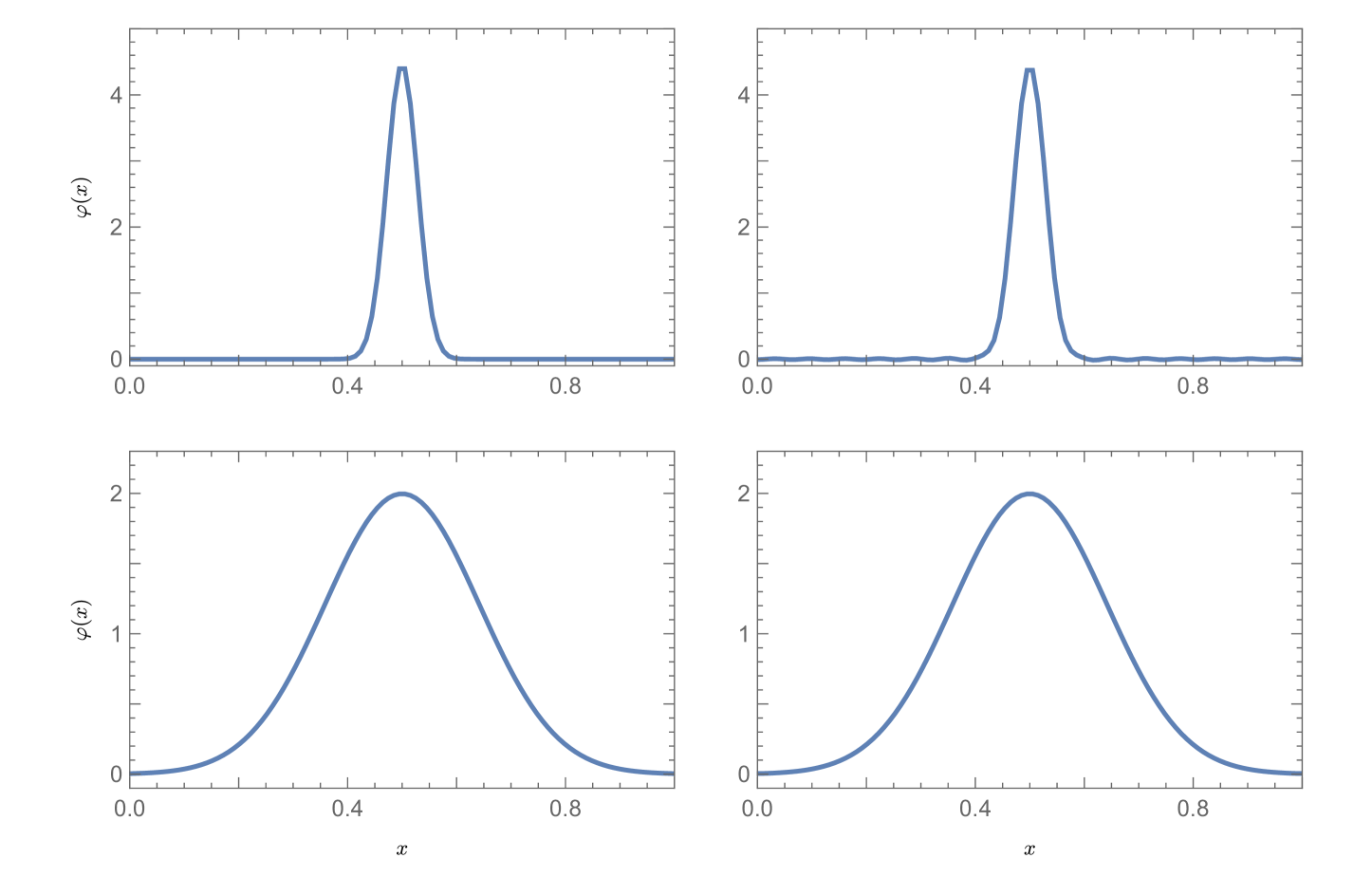
Figure S1: Original atomic wavepacket (left column) compared with those from reconstruction (right column). The top row is for $w=0.02$, while the second row is for $w=0.1$.

Note that as we have omitted the sine term and truncated at $n_{c}$, these will affect the atomic wavepacket reconstructed after TWA simulation, especially when the wavepacket width is small. This is indicated in Fig. S1, in which we compared the original wavepacket with the reconstructed one. However this only cause quantitative differences and will not affect our main results in the text.

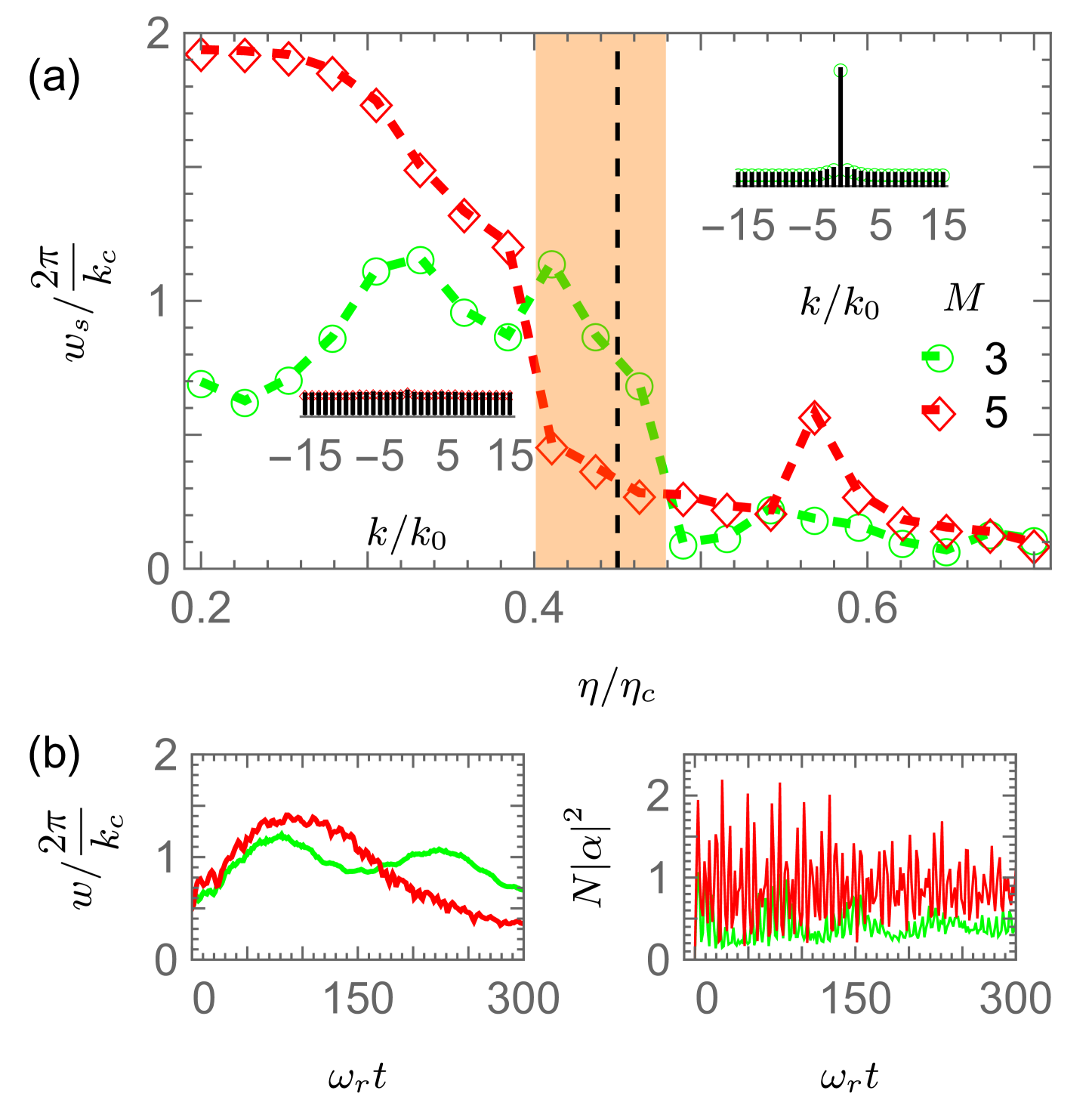
Figure S2: Quantum diffusion dynamics calculated with TWA. (a) Atom wavepacket width at steady state $w_{s}$ versus pumping strength $\eta$. In the shaded region $w_{s}$ at $M=3$ is larger than that at $M=5$, with the insets demonstrating localized (extended) atomic momentum distribution for $M=3$ ($5$) respectively at a $\eta$ marked by the black dashed line. The corresponding evolution dynamics of atomic wavepacket width $w$ and cavity photon number are given in (b). The parameters are the same as those in the main text.

With periodic boundary condition considered here, as shown in Fig. S2(b), the width increases at initial time and then gradually approaches a steady value. In the meanwhile, the cavity photon number jump from zero before reaching saturation. We plot the steady state width $w_{s}$ versus the pumping strength in Fig. S2(a). As expected, since the lattice constant becomes larger with increased $M$, one will have broader wavepacket in the $M=5$ case as compared with $M=3$ for an initial identical wavepacket. This is true at small $\eta$. $w_{s}$ abruptly decreases upon the pumping strength passing across a critical value. This diffusion behavior tuned between two distinct diffusive regimes arises from superradiant phase transitions: (i) For small pumping strengths, cavity field is not excited and atomic wavepacket spreads until it reach the unit cell boundary, with the width showcasing damped oscillation as illustrated by the green line in Fig. S2(b). In the steady state, atomic wavefunction distribution is localized in momentum space as shown in the upright inset of Fig. S2(a), indicating extended distribution in coordinate space. (ii) While at large pumping, intracavity field build up to coform a moiré lattice. Different atomic momentum modes are populated via scattering, resulting in momentum space extended distribution at steady state (downleft inset of Fig. S2(a)), and henceforce suppressed expansion and width.

Noteworthy that in the shaded region of Fig. S2(a), for the very same pumping strength, one counter-intuitively have larger $w_{s}$ in the $M=3$ case instead of $M=5$. In this specific parameter region, atomic wavepacket diffuse in distinct different manner determined by the moiré parameter: In the $M=3$ case atomic diffusion behavior can be depicted by (i), while the atomic diffusion in the $M=5$ case is attributed to (ii). This completely opposite behavior is manipulated solely by a change in $M$ with all the other physical parameters identical, thus can be regarded as moiré effect. One can understand this phenomenon as the result of interplay between quantum interference (Anderson localization) and quantum fluctuations of the cavity field. The aid of cavity is indispensable to observe the moiré effect.