TamedPUMA: safe and stable imitation learning
with geometric fabrics

Abstract

Using the language of dynamical systems, Imitation learning (IL) provides an intuitive and effective way of teaching stable task-space motions to robots with goal convergence. Yet, IL techniques are affected by serious limitations when it comes to ensuring safety and fulfillment of physical constraints. With this work, we solve this challenge via TamedPUMA, an IL algorithm augmented with a recent development in motion generation called geometric fabrics. As both the IL policy and geometric fabrics describe motions as artificial second-order dynamical systems, we propose two variations where IL provides a navigation policy for geometric fabrics. The result is a stable imitation learning strategy within which we can seamlessly blend geometrical constraints like collision avoidance and joint limits. Beyond providing a theoretical analysis, we demonstrate TamedPUMA with simulated and real-world tasks, including a 7-DoF manipulator. https://autonomousrobots.nl/paper_websites/pumafabricsLink to website

1 Introduction

As robotic solutions rapidly enter unstructured environments such as the agriculture sector and homes, there is a critical need for methods that allow non-experts to easily adapt robots for new tasks. Currently, experts manually program these tasks, a method that is costly and not scalable for widespread use. Moreover, these sectors demand that robots safely interact with dynamic environments where humans are present.

A possible solution to this societal challenge comes from Imitation Learning (IL). Using this technique, robots can learn motion profiles from demonstrations provided by non-expert users. Furthermore, by encoding the learned trajectories as solutions of a dynamical system, established mathematical tools from dynamical system theory can be used to guarantee convergence to the task’s goal state, as we discuss more in detail in Sec. 1.1. In a robotics context, these learned dynamical systems commonly encode the navigation policy towards a goal within a task space - such as the evolution of the end-effector pose of a manipulator while pouring water in a glass from all possible initial locations. However, this focus on task space motions renders IL fundamentally limited when considering physical constraints involving the robot’s body impacting itself or interacting with the external environment. Substantial recent research has looked into the problem but, as we discuss in Sec. 1.1, to the best of our knowledge, no IL method can simultaneously ensure stability and real-time fulfillment of physical constraints for systems with many degrees of freedom.

This work contributes to the state of the art by introducing TamedPUMA, a learning framework that builds on IL and geometric fabrics (Ratliff et al., 2020) to obtain inherently stable and safe motion primitives from demonstrations. By leveraging the recently introduced geometric framework for motion generation called geometric fabrics, our approach learns stable motion profiles while considering online whole-body collision-avoidance and joint limits. To make this possible, the learned task-space policy has to be formulated as a ${2^{\mathrm{nd}}\text{-order}}$ (neural) dynamical system as fabrics operate within the Finsler Geometry framework where vector fields must be defined at the acceleration level (Bao et al., 2012). Also, the learned policy must admit an aligned potential, which roughly means a scalar function whose gradient is aligned with the acceleration field when the velocity is null. In this paper, we formally assess how we can ensure that both conditions are met. The performance of our approach is evaluated with a simulated and real-world 7-DoF manipulator, where we also benchmark it against vanilla geometric fabrics, vanilla learned stable motion primitives and a modulation-based IL approach leveraging collision-aware IK.

1.1 Related work

Learning stable dynamical systems from demonstrations Multiple methodologies have been introduced for learning stable dynamical systems (Billard et al., 2022; Hu et al., 2024). An influential methodology in learning stable dynamical systems is Dynamical Movement Primitives (DMP) by Ijspeert et al. (2013), ensuring convergence towards a simple manually-designed dynamical system. This approach is extended to non-Euclidean state spaces (Ude et al., 2014), probabilistic environments (Li et al., 2023; Przystupa et al., 2023), and in the context of deep neural network (DNN) (Pervez et al., 2017; Ridge et al., 2020). To ensure stability, several approaches enforce a specific structure on the function approximators, such as enforcing positive or negative definiteness (Khansari-Zadeh and Billard, 2011; Lemme et al., 2014; Fernandez and Billard, 2018), or invertibility (Perrin and Schlehuber-Caissier, 2016; Rana et al., 2020; Urain et al., 2020). In contrast, Pérez-Dattari and Kober (2023); Pérez-Dattari et al. (2024) enforce stability via additional loss functions derived using tools from the deep metric learning literature (Kaya and Bilge, 2019). Importantly,  Pérez-Dattari et al. (2024) extends the ideas of Pérez-Dattari and Kober (2023) to more general scenarios, achieving better results in non-Euclidean state spaces and ${2^{\mathrm{nd}}\text{-order}}$ dynamical systems. These two features are essential for integrating such frameworks with fabrics, which, to the best of our knowledge, have not been simultaneously demonstrated in other works using time-invariant formulations, e.g. Rana et al. (2020); Mohammadi et al. (2024); Saveriano et al. (2023).

From IL to whole-body motion generation For the safe operation of robots around humans, not only the dynamical system acting as the navigation policy should be stable but the whole-body motion is desired to be stable, collision-free, and within the system limits. However, most existing IL solutions that incorporate obstacle avoidance when learning dynamical systems in end-effector space focus solely on avoiding collisions with the end-effector, e.g. Mohammadi et al. (2024); Ginesi et al. (2019); Huber et al. (2023). One possibility to achieve full-body collision avoidance in such cases is by employing collision-aware Inverse Kinematics (IK) solvers (Tedrake, 2023; Rakita et al., 2021). Nevertheless, this ignores the desired acceleration or velocity profile specified by the learned dynamical system.

Another strategy is to combine IL with an optimization-based motion planner such as Model Predictive Control (MPC), inheriting the possibility to include kinodynamic and safety constraints and including the learned policy in the cost function. Several combinations exist, such as augmenting the cost function with a learned policy (Xiao et al., 2022), learning the complete cost function (Tagliabue and How, 2023), and learning the complete MPC framework (Ahn et al., 2023). Hu et al. (2023) propose MPDMP⁺ as a fast alternative for navigation amongst dynamic obstacles, combining DMPs with MPC where the cost function merges multiple demonstrations and includes obstacle avoidance using potential functions. Although some IL-MPC frameworks can guarantee stability (Ahn et al., 2023; Hewing et al., 2020), where most methods lack these guarantees, their applications remain limited with no demonstrations in real-world robotics.

Geometric motion generation A fast alternative strategy to optimization-based motion planners lies in the field of geometric motion generation. These techniques are inspired by Operational Space Control (Khatib, 1987), achieving stable and converging behavior for kinematically redundant robots using differential geometry (Bullo and Lewis, 2019). Recently, Riemannian Motion Policies and its extension, Geometric Fabrics, have been introduced (Ratliff et al., 2018; Ratliff and Van Wyk, 2023). In Geometric Fabrics, convergence is guaranteed with simple construction rules (Ratliff et al., 2020; Xie et al., 2020) and is also extended to dynamic environments (Spahn et al., 2023). These policies are shown to be beneficial in designing human-like motions (Klein et al., 2022) and have a high planning frequency compared to optimization-based methods (Spahn et al., 2023).

Combining geometric motion generation and learning Geometric methods have been considered in conjunction with reinforcement learning (Van Wyk et al., 2023) and Bayesian learning (Jaquier et al., 2020). Most interestingly for the present work, Xie et al. (2021, 2023) have looked into combining fabrics with IL. The method they propose is essentially different from TamedPUMA, as they directly learn the fabric, which results in limitations in terms of motion expressiveness.

2 Preliminaries

In this section, fundamental concepts are introduced for trajectory generation using artificial dynamical systems. Firstly, task and configuration spaces and their relations are specified in Section 2.1, followed by an overview of motion generation using geometric fabrics in Section 2.2. For a detailed overview of geometric fabrics and differential geometries, we refer the reader to Ratliff et al. (2020); Ratliff and Van Wyk (2023). Section 2.3 provides the necessary background on learned stable motion primitives and its stability properties.

2.1 Configuration and task spaces

The configuration of the robot is denoted by $\bm{q}\in\mathcal{C}$ with its time derivatives $\dot{\bm{q}}$ and $\ddot{\bm{q}}$. Here, $\mathcal{C}$ indicates the configuration space of the robot, which has a dimension of $n$. Tasks can be defined in different task spaces $\mathcal{X}_{j}$. For instance, collision avoidance of a manipulator’s end effector can be a task defined in the end-effector’s space. Additionally, to address whole-body obstacle avoidance, multiple tasks can be defined for various coordinates along the robot’s body. Furthermore, other tasks, such as reaching behaviors, can also be included. A task variable $\bm{x}_{j}\in\mathcal{X}_{j}$ denotes the value of the state representation for the $j$-th task space, where $j\in[M]$, $M$ denotes the number of task spaces, and $[M]=\{j\in\mathbb{Z}^{+}:j\leq M\}$. The relation between the configuration space and a given task space is stated via a twice-differential map $\phi_{j}:\mathcal{C}\to\mathcal{X}_{j}$, and the map’s Jacobian as $\bm{J}_{\phi_{j}}=\frac{\partial\phi_{j}}{\partial\bm{q}}$.

2.2 Geometric fabrics

A dynamical system describes the behavior of a system using differential equations. In geometric fabrics (Ratliff et al., 2020), these dynamical systems describe an artificial system generating desired trajectories for a robotic system. The desired motions are described using second-order nonlinear time-invariant dynamical systems, $\ddot{\bm{x}}=f(\bm{x},\dot{\bm{x}})$. In this framework, dynamical systems consist of two parts: one that conserves a Finsler energy and another that is energy-decreasing. The energy-conservative part takes care of all avoidance tasks, e.g., joint limit avoidance and obstacle avoidance, while the energy-decreasing part drives the system towards the goal.

Let us first focus on the energy-conservative dynamical system. The behavior for an avoidance task is described using a second-order dynamical system, $\bm{M}(\bm{x},\dot{\bm{x}})\ddot{\bm{x}}+\bm{\xi}(\bm{x},\dot{\bm{x}})=\bm{0}$ within a task space $\mathcal{X}$ where $\bm{M}(\bm{x},\dot{\bm{x}})$ is symmetric and invertible. If this system, often referred to as a spectral semi-spray $\bm{h}:\mathcal{S}=\left(\bm{M},\bm{\xi}\right)_{\mathcal{X}}$, is conserving a Finsler energy, it is called a fabric $\tilde{\bm{h}}:\mathcal{S}=(\tilde{\bm{M}},\tilde{\bm{\xi}})_{\mathcal{X}}$ (Ratliff et al., 2020). The system $\bm{h}$ is transformed into a fabric $\tilde{\bm{h}}$ through energization with the Finsler energy, i.e., ${\tilde{\bm{h}}=\mathrm{energize}_{\mathcal{L}_{e}}[\bm{h}(\bm{x},\dot{\bm{x}})]}$ (Eq. 13 in Ratliff and Van Wyk (2023)). Notably, the system’s energization only changes the speed along the path, but not the path itself, if the system is homogeneous of Degree 2, i.e., $\bm{h}(\bm{x},\alpha\dot{\bm{x}})=\alpha^{2}\bm{h}(\bm{x},\dot{\bm{x}}),\ \forall\alpha\geq 0$.

Each avoidance task can be described by these energy-conservative fabrics, $\ddot{\bm{x}}_{j}=\tilde{\bm{h}}(\bm{x}_{j},\dot{\bm{x}}_{j})$, within their own task space $\mathcal{X}_{j}$. To construct a whole-body policy for the robotic system, multiple task-space fabrics are mapped to the configuration space using a pullback operation and summed. The pullback operation, $\mathrm{pull}_{\phi_{j}}\left(\tilde{\bm{M}}_{j},\tilde{\bm{\xi}}_{j}\right)_{\mathcal{X}_{j}}={\left(\bm{J}^{T}_{\phi_{j}}\tilde{\bm{M}}_{j}\bm{J}_{\phi_{j}},\bm{J}^{T}_{\phi_{j}}(\tilde{\bm{\xi}}_{j}+\dot{\bm{J}}_{\phi_{j}}\dot{\bm{q}})\right)}_{\mathcal{C}}$, is constructed as a function of $\phi_{j}$, and maps the energy-conserving fabric to the configuration space, resulting in the system $\tilde{\bm{h}}_{j}(\bm{q},\dot{\bm{q}}):\mathcal{S}_{j}=(\tilde{\bm{M}}_{j},\tilde{\bm{\xi}}_{j})_{\mathcal{C}}$. The specs in $\mathcal{C}$ are summed, e.g. $(\mathcal{S}_{1}+\mathcal{S}_{2})_{\mathcal{C}}=(\tilde{\bm{M}}_{1}+\tilde{\bm{M}}_{2},\tilde{\bm{\xi}}_{1}+\tilde{\bm{\xi}}_{2})_{\mathcal{C}}$ where the resulting dynamical system $\ddot{\bm{q}}=\tilde{\bm{h}}(\bm{q},\dot{\bm{q}})$ is a fabric as well, since the summation and pullback operations are closed under algebra. This combined fabric can be forced towards the minimum of a potential $\bm{\psi}(\bm{q})\in\mathbb{R}$ and damped with a positive definite damping matrix (Ratliff et al., 2020). On a more abstract level, the desired dynamical system can be denoted as a combination of energy-conserving fabric $\tilde{\bm{h}}$ and an energy-decreasing navigation policy $\bm{f}$ which is damped,

$$\ddot{\bm{q}}=\tilde{\bm{h}}(\bm{q},\dot{\bm{q}})+\bm{f}(\bm{q},\dot{\bm{q}}).$$ (1)

2.3 Learning stable motion primitives via PUMA

Similarly to geometric fabrics, Policy via neUral Metric leArning (PUMA) models a desired motion as a nonlinear time-invariant dynamical system. This method represents the dynamical system $\bm{f}^{\mathcal{T}}_{\theta}$ in one of the task spaces $\mathcal{X}_{j}$ (commonly the robot’s end effector’s space), denoted as $\mathcal{T}$, as a DNN with weights $\theta$. The weights are optimized to imitate a set of demonstrations while ensuring convergence to a goal state $\bm{x}_{\text{g}}\in\mathcal{T}$ (Pérez-Dattari et al., 2024; Pérez-Dattari and Kober, 2023). In other words, $\bm{x}_{\text{g}}$ must be a globally asymptotically stable equilibrium in the region of interest.

To enforce stability under minimization of the loss function, a specialized loss is introduced and optimized alongside an imitation loss. To design this loss, it is necessary first to define a latent space $\mathcal{L}$ as the output of a hidden layer $l$ of the DNN, such that

$$\ddot{\bm{x}}=\bm{f}_{\theta}^{\mathcal{T}}(\bm{x},\dot{\bm{x}})=\bm{\varphi}_{\theta}(\bm{\rho}_{\theta}(\bm{x},\dot{\bm{x}})),$$ (2)

where $\bm{\rho}_{\theta}:\mathcal{T}\to\mathcal{L}$ encodes the first $1,...,l$ layers and $\bm{\varphi}_{\theta}:\mathcal{L}\to d\mathcal{T}$ the last $l+1,...,L$ layers with $d\mathcal{T}$ representing the tangent bundle of $\mathcal{T}$, capturing the derivatives and tangent spaces associated with $\mathcal{T}$. Then, a mapped system $\bm{f}^{\mathcal{T}\rightarrow\mathcal{L}}_{\theta}(\bm{x},\dot{\bm{x}})$ can be defined in $\mathcal{L}$ as

$$\ddot{\bm{y}}=\bm{f}^{\mathcal{T}\rightarrow\mathcal{L}}_{\theta}(\bm{x},\dot{\bm{x}})=\frac{\partial\bm{\rho}_{\theta}(\bm{x},\dot{\bm{x}})}{\partial t}.$$ (3)

These definitions enable the formulation of the stability conditions introduced in Pérez-Dattari and Kober (2023), which can be stated as:

Theorem 2.1 (Stability conditions (Pérez-Dattari et al., 2024)).

In the region $\mathcal{T}$, $\bm{x}_{\mathrm{g}}$ is a globally asymptotically stable equilibrium of $\bm{f}_{\theta}^{\mathcal{T}}$ if, $\forall\bm{x}\in\mathcal{T}$, (1) $\bm{y}_{\mathrm{g}}=\bm{\rho}_{\theta}(\bm{x}_{\mathrm{g}})$ is a globally asymptotically stable equilibrium of $\bm{f}_{\theta}^{\mathcal{T}\to\mathcal{L}}$, and (2) $\bm{\rho}_{\theta}(\bm{x})=\bm{y}_{\mathrm{g}}\Rightarrow\bm{x}=\bm{x}_{\mathrm{g}}$.

These conditions can be enforced via the following loss (Pérez-Dattari et al., 2024):

$$\ell_{\text{stable}}=\sum_{\bm{y}_{0}\in\mathcal{B}}\sum_{t\in\mathcal{H}}\max(0,m+d(\bm{y}_{\mathrm{g}},\bm{y}(\bm{y}_{0},t+\Delta t))-d(\bm{y}_{\mathrm{g}},\bm{y}(\bm{y}_{0},t))),$$ (4)

where $d(\cdot,\cdot)$ is a distance function, $m$ is a small margin hyperparameter, and $\bm{y}(\bm{y}_{0},t)$ represents the value of $\bm{y}$ for an initial condition $\bm{y}_{0}$ and time $t$. Here, $\mathcal{B}$ is a batch of initial conditions obtained at every iteration by randomly sampling the workspace $\mathcal{T}$, and $\mathcal{H}$ contains different values of $t$ up to some time horizon $T$. To imitate the set of demonstrations, this method minimized the combined loss $\ell_{\textrm{PUMA}}=\ell_{\textrm{IL}}+\lambda\ell_{\textrm{stable}}$, where $\ell_{\textrm{IL}}$ is the behavioral cloning loss employed in Pérez-Dattari and Kober (2023) and $\lambda$ is a weight factor.

3 TamedPUMA: Combining learned stable motion primitives and fabrics

With learned stable motion primitives, complex tasks can be learned from demonstrations, while converging to the goal. In TamedPUMA, these learned dynamical systems are incorporated into the framework of geometric fabrics, generating stable and safe motions while respecting whole-body collision avoidance and physical constraints of the robot. In Section 3.1, the problem formulation is discussed, followed by the two variations of TamedPUMA, the Forcing Policy Method (FPM) and Compatible Potential Method (CPM), in Section 3.2 and  3.3 respectively.

3.1 Problem formulation

Consider there exists a dynamical system $\tilde{\bm{f}}$ that describes a desired motion profile for a robot, which induces the distribution of trajectories $\tilde{p}(\tau)$. For a given task variable $\bm{x}\in\mathcal{T}$, such as the robot’s end-effector pose, we assume we can sample trajectories from this distribution. Then, if the dynamical system $\bm{f}^{\mathcal{T}}_{\theta}$ represents the evolution of the robot’s state in $\mathcal{T}$, our objective is to minimize the distance between the distribution of trajectories induced by this system $p_{\theta}(\tau)$ and $\tilde{p}(\tau)$. Furthermore, $\bm{f}^{\mathcal{T}}_{\theta}$ must always reach a desired state $\bm{x}_{\mathrm{g}}\in\mathcal{T}$ while accounting for region avoidance constraints, namely, self-collisions, obstacles, and joint limits for M tasks defined in multiple task spaces $\mathcal{X}_{j}$. More formally,

$$\ \bm{f}^{\mathcal{T}*}_{\theta} =\underset{\bm{f}^{\mathcal{T}}_{\theta}}{\arg\min}\ D_{\text{KL}}\left(\tilde{p}(\tau)||p_{\theta}(\tau))\right),$$ (5a)

s.t. $$\ \ \ \lim_{t\to\infty}||\bm{x}-\bm{x}_{\mathrm{g}}||=0,\ \ \ \forall\bm{x}\in\mathcal{T},$$ (5b)

$$\ \ \ \bm{x}_{j}\in\mathcal{X}_{j}^{\text{free}},\ \ \ \ \ \ \ \ \ \ \ \ \ \ \ \ \ \ \forall j\in[M].$$ (5c)

This objective minimizes the Kullback-Leibler divergence between the estimated dynamical system and the target system (5a). This divergence is often used as a distance measure between distributions as it is minimized through maximum likelihood estimation using distribution samples (Osa et al., 2018). Moreover, the problem is subject to two constraints: (5b) the dynamical system should converge to a task-space goal $\bm{x}_{\mathrm{g}}$ in $\mathcal{T}$, and (5c) task-space states $\bm{x}_{j},\forall j\in[M]$, should remain within the free space $\mathcal{X}_{j}^{\text{free}}$ where the dynamical system is well-defined, which could be the collision-free space or the space within the joint limits.

From this formulation, PUMA softly addresses (5a) using the loss $\ell_{\textrm{IL}}$, while fabrics addresses (5c) through their geometric-aware formulation. Both approaches tackle the problem of stability; however, it remains challenging to combine both methods while ensuring convergence to the goal (5b). In the following subsections, we propose two approaches to address this.

3.2 The Forcing Policy Method (FPM)

First, we introduce the FPM. For this purpose, we define the dynamical system $\bm{f}^{\mathcal{C}}_{\theta}$ in configuration space resulting from applying a pullback operation, via PUMA, in $\mathcal{T}$:

$$\ddot{\bm{q}}_{\text{DNN}}=\bm{f}^{\mathcal{C}}_{\theta}(\bm{q},\dot{\bm{q}})=\mathrm{pull}_{\phi_{\mathcal{T}}}\left(\bm{f}^{\mathcal{T}}_{\theta}(\bm{x}_{\text{ee}},\dot{\bm{x}}_{\text{ee}})\right),$$ (6)

where the task variable $\bm{x}_{\text{ee}}$ is the end-effector position and orientation of the robot as illustrated in Fig. 1. Then, leveraging the definition of a forced system from Eq. (1), in the FPM we propose to use the pulled system obtained via PUMA as the forcing policy,

$$\ddot{\bm{q}}^{\text{d}}=\tilde{\bm{h}}(\bm{q},\dot{\bm{q}})+\bm{f}^{\mathcal{C}}_{\theta}(\bm{q},\dot{\bm{q}}).$$ (7)

Assuming $\ell_{\textrm{PUMA}}$ has already been minimized, the system $\bm{f}^{\mathcal{T}}_{\theta}$ comes to rest at $\bm{x}_{\mathrm{g}}$, implying that $\bm{f}^{\mathcal{C}}_{\theta}$ converges to $\bm{q}_{\mathrm{g}}$ where multiple values of $\bm{q}_{\mathrm{g}}$ may exist in the case of a redundant system. This collection of states $\bm{q}_{\mathrm{g}}$ corresponds to the zero set of $\bm{f}^{\mathcal{C}}_{\theta}$. From Proposition II.17 in Ratliff and Van Wyk (2023), we know that if the system in Eq. (7) reaches the zero set of $\bm{f}^{\mathcal{C}}_{\theta}$, it will stay there (which comes from the observation that fabrics are conservative). However, convergence of Eq. (7) to the zero set of $\bm{f}^{\mathcal{C}}_{\theta}$ is not formally assessed. Re-evaluating the problem formulation suggests that the constraint in Eq (5b), stating that the system should converge to the desired minimum $\bm{q}_{\mathrm{g}}$, is therefore not guaranteed. In Sec. 3.3, we propose a method with stronger convergence guarantees.

Figure 1: This illustration of TamedPUMA shows the behavior design given the relationships between the different task and configuration-space variables. The joint angles and velocities get mapped into task space where the desired behavior is specified. Via fabrics, all avoidance behaviors are defined using the joint limits, and varying obstacle positions, e.g. the position of the bowl. The DNN captures the desired behavior of the end-effector position and orientation.

3.3 The Compatible Potential Method (CPM)

As a second approach, we propose the CPM leveraging compatible potentials to obtain a stronger notion of convergence. For a potential function compatible with a dynamical system, its negative gradient generally points in the same direction as the system’s vector field. More formally:

Definition 3.1 (Compatible potential (Ratliff and Van Wyk, 2023)).

A potential function $\psi$ is compatible with $\bm{f}$ if: (1) ${\partial\psi(\bm{q})=\bm{0}}$ if and only if $\bm{f}(\bm{q},\bm{0})=\bm{0}$, and (2) $-\partial\psi^{\top}\bm{f}(\bm{q},\bm{0})>\bm{0}$ wherever $\bm{f}(\bm{q},\bm{0})\neq\bm{0}$.

Building upon this, Theorem III.5 in Ratliff and Van Wyk (2023) states that given a dynamical system $\bm{f}$ with a compatible potential, it is possible to construct another system that converges to the zero set of $\bm{f}$. Crucially, this new system can incorporate the avoidance behaviors (e.g., joint limits and collision avoidance) in configuration space, represented by $\bm{h}(\bm{q},\dot{\bm{q}})=\sum_{j=1}^{M}\bm{h}_{j}(\bm{q},\dot{\bm{q}})$, as:

$$\ddot{\bm{q}}^{\text{d}}=\textrm{energize}_{\mathcal{H}}[\bm{h}+\bm{f}]+\gamma(\bm{q},\dot{\bm{q}})\ \ \ \text{with}\ \ \ \gamma(\bm{q},\dot{\bm{q}})=-\left(\frac{\dot{\bm{q}}\dot{\bm{q}}^{\top}}{\dot{\bm{q}}^{\top}\bm{M}_{\mathcal{L}_{e}}\dot{\bm{q}}}\right)\partial\psi-\beta\dot{\bm{q}}.$$ (8)

Here, we assume that the metric $\bm{M}_{\mathcal{L}_{e}}$ is bounded in a finite region, strictly positive definite everywhere and does not vanish or reduce rank if $\dot{\bm{q}}\rightarrow\bm{0}$, $\beta>0$, and obstacle positions and joint limits are static. Consequently, we aim to leverage this result by using $\bm{f}^{\mathcal{C}}_{\theta}$ as the system $\bm{f}$ in Eq. (8) with the compatible potential. From the previous section, we already defined that the zero set of this system maps to the equilibrium $\bm{x}_{\mathrm{g}}\in\mathcal{T}$. Hence, it remains to find a compatible potential for this function to employ the result from Theorem III.5.

Notably, if (4) is successfully minimized, it is possible to design a compatible potential for the system $\bm{f}^{\mathcal{T}}_{\theta}$ in the latent space $\mathcal{L}$ using the mapping $\bm{\rho}_{\theta}$ by setting $\dot{\bm{x}}=\bm{0}$. Specifically, we can construct a potential using the latent-space variable $\bm{y}$ and the encoder $\bm{\rho}_{\theta}$ of PUMA as in Eq. (2),

$$\psi(\bm{x})=\|\bm{y}_{\mathrm{g}}-\bm{y}\|^{2}=\|\bm{\rho}_{\theta}(\bm{x}_{\mathrm{g}},\bm{0})-\bm{\rho}_{\theta}(\bm{x},\bm{0})\|^{2}.$$ (9)

To observe that this is a compatible potential of $\bm{f}^{\mathcal{T}}_{\theta}$, first, we highlight that since $\bm{x}_{\mathrm{g}}$ is asymptotically stable, we have ${\partial\psi(\bm{x}_{\mathrm{g}})=\bm{0}}$ if and only if ${\bm{f}(\bm{x}_{\mathrm{g}},\bm{0})=\bm{0}}$. This satisfies the first condition of Definition 3.1. Second, we note that for all $\bm{x}\neq\bm{x}_{\mathrm{g}}$, Equation (4) ensures that the value of $\psi(\bm{x})$ decreases as $\bm{f}^{\mathcal{T}}_{\theta}$ evolves over time, except for some edge cases that could, in theory, occur if $\bm{\rho}_{\theta}$ has a large Lipschitz constant. These edge cases can be eliminated through regularization. Thus, this potential also satisfies the second condition of Definition 3.1 and therefore $\psi(\bm{x})$ is a compatible potential of $\bm{f}_{\theta}^{\mathcal{T}}$. Finally, for Eq. 8 it only remains to express the gradient of this potential in configuration space, previously denoted as $\partial\psi$. For clarity, we will henceforth write this as $\partial\psi/\partial\bm{q}$. To achieve this, we require the forward kinematics from configuration space $\mathcal{C}$ to task space $\mathcal{T}$, denoted $\phi^{\mathcal{T}}$. Then, we obtain

$$\partial\psi=\frac{\partial\psi}{\partial\bm{q}}=\frac{\partial\psi}{\partial\bm{x}}\cdot J_{\phi^{\mathcal{T}}}(\bm{x}),$$ (10)

where $J_{\phi^{\mathcal{T}}}$ is the Jacobian matrixof the forward kinematics, commonly available in robotic frameworks. The term $\partial\psi/\partial\bm{x}$ can be approximated via automatic differentiation tools for DNNs.

Assumptions on $\bm{M}_{\mathcal{L}_{e}}$ To conclude this section, it is relevant to discuss further the implications of the assumptions on $\bm{M}_{\mathcal{L}_{e}}$. For a fabric describing collision avoidance, two cases exist as the spec describing the fabric must be boundary conforming (Ratliff et al., 2020). (1) The metric $\bm{M}_{\mathcal{L}_{e}}$ is finite along the eigen-directions parallel to the boundary’s tangent space but goes to infinity along directions orthogonal to the tangent space. (2) The metric $\bm{M}_{\mathcal{L}_{e}}$ is a finite matrix along all trajectories, implying that $\bm{M}_{\mathcal{L}_{e}}$ is also finite in the limit when $t\rightarrow\infty$. Considering our previous assumptions on $\bm{M}_{\mathcal{L}e}$ for (8), i.e. the metric is bounded in a finite region and strictly positive definite everywhere, we can design fabrics only according to the second scenario. This implies that, in the limit, we ensure convergence to the zero set of the forcing policy $\bm{f}^{\mathcal{C}}_{\theta}(\bm{q},\dot{\bm{q}})$; however, collision avoidance is not guaranteed in the limit, as barrier-like functions that go to infinity on the boundary cannot be used to construct $\bm{M}_{\mathcal{L}_{e}}$. For more details, we refer the reader to the attached material.

4 Experimental Results

In this section, we explore TamedPUMA’s capabilities in constructing stable and collision-free motions for a 7-DOF manipulator. Details regarding the DNN, differential mappings, a discussion on the limitations, code and videos are included in the attached material.

4.1 Experimental setup and performance metrics

To show the performance of the two variations of TamedPUMA, FPM and CPM, simulations using the Pybullet physics simulation (Coumans and Bai, 2016) and real-world experiments are performed on a 7-DoF KUKA iiwa manipulator. Two tasks are analyzed, picking a tomato from a crate and pouring liquid from a cup, where a DNN is trained for each task using 10 demonstrations, recording end-effector positions, velocities and accelerations. The proposed FPM and CPM, are compared against vanilla geometric fabrics, vanilla PUMA and modulation-IK. Modulation-IK modifies PUMA to be obstacle-free within the task space using a modulation matrix (Khansari-Zadeh and Billard, 2012). Then, whole-body collision avoidance is achieved by tracking the modified desired pose using a collision-aware IK (Tedrake, 2023). All methods are evaluated based on their success rate and time-to-success, which respectively indicate the ratio of successful scenarios and the time required for the robot to reach the goal pose. Successful scenarios ensure collision-free motions with an end pose satisfying $\left\lVert\bm{x}_{\text{ee}}-\bm{x}_{\text{g}}\right\rVert_{2}<0.05\ m$. In addition, the computation time is denoted, and the path difference to the desired path by PUMA as $\frac{1}{P}\sum\left\lVert\bm{x}_{\text{ee}}-\bm{x}_{\text{PUMA}}\right\rVert_{2}$ where $\bm{x}_{\text{ee}}$ and $\bm{x}_{\text{PUMA}}$ correspond to the end-effector poses along the path with length $P$ of the analyzed method and PUMA respectively. The path difference is computed in obstacle-free scenarios, where we aim to track the DNN as closely as possible, and in obstacle-rich allowing for deviations from this path.

4.2 Simulation experiments on a 7-DOF manipulator

Table 1: Statistics for 30 simulated scenarios. The path difference to PUMA is measured in an obstacle-free environment, while all other metrics are compared in an obstacle-rich environment.

	Success-Rate	Time-to-Success [s]	Computation time [ms]	Path difference to PUMA
PUMA	0.40	4.75 $\pm$ 1.31	4.41 $\pm$ 0.26	0
Modulation-IK	0.57	5.75 $\pm$ 5.83	7.08 $\pm$ 5.98	0.39 $\pm$ 0.42
Fabrics	0.83	8.18 $\pm$ 5.54	0.39 $\pm$ 0.03	0.22 $\pm$ 0.27
FPM (ours)	1.00	6.97 $\pm$ 3.78	5.22 $\pm$ 0.22	0.02 $\pm$ 0.04
CPM (ours)	1.00	7.01 $\pm$ 3.57	6.55 $\pm$ 0.96	0.04 $\pm$ 0.06

In simulation, 30 realistic scenarios are explored, including 15 scenarios of a tomato-picking task and 15 scenarios of a pouring task. In each task, the initial robot configuration and obstacle locations change. Moreover, 10 scenarios included moving goals, and 7 scenarios included moving obstacles. For each scenario, at least one obstacle is situated between the initial configuration and the goal pose. The last five links on the robotic chain are considered for collision avoidance, given that the first three links have restricted movement due to the base being mounted to the table. The shape of the last five links is approximated using spheres with a radius of 9 $cm$, and 7 $cm$ for the final link.

As depicted in Table 1, the two TamedPUMA variations improve the success rate over PUMA by enabling whole-body obstacle avoidance. In contrast to geometric fabrics, FPM and CPM can track the desired motion profile leading to a smaller path difference with PUMA of 0.02 $\pm$ 0.04 and 0.04 $\pm$ 0.06 respectively, compared to geometric fabrics, 0.22 $\pm$ 0.27, in an obstacle-free environment. In an obstacle-rich environment, geometric fabrics result in a deadlock in 6 of the 30 scenarios where the robot does not reach the goal as it is unable to move around the edge of the crate or object. The benchmark Modulation-IK is also unable to achieve all tasks due to collisions or deadlocks, as it cannot find a feasible solution converging towards the goal. TamedPUMA thereby inherits the efficient scalability to multi-object environments from fabrics, as computation time in an environment with 1000 obstacles is only 5.9 $\pm$ 0.8 $ms$ and 7.0 $\pm$ 1.1 $ms$ for FPM and CPM respectively, a neglectable increase with respect to the two obstacles considered in Table 1, while optimization-based methods like Modulation-IK scale poorly with large numbers of obstacles with a computation time of 3.5$\cdot 10^{3}$ $\pm$ 10.7$\cdot 10^{3}$ $ms$ in an environment with 1000 obstacles. Although CPM offers stronger theoretical guarantees than FPM, performance is similar (see Table 1). Even though we do not optimize over the time-to-success, both FPM and CPM achieve the task within a reasonable time while remaining collision-free. Computation times are 4-7 $ms$ on a standard laptop (i7-12700H) making the methodologies well suitable for real-time reactive motion generation in dynamic environments.

4.3 Real-world experiments on a 7-DOF manipulator

Experiments are performed on the real 7-DOF for the tomato-picking and pouring task where all obstacles, e.g. a bowl, a person’s hand and a helmet, are dynamically tracked in real-time via an optitrack system and modeled as spheres. In addition to the collision spheres considered during simulation, a collision sphere is added to the collision geometry on the center of the robotic hand with a diameter of 14 $cm$. The desired actions by TamedPUMA are sent at 30 Hz to a joint impedance controller running at 1000 Hz. Snapshots of a real-world experiment of the CPM are illustrated in Fig. 2, Fig. 3 and Fig 4, and the videos in the attached material show several movements for the simulated and real-world experiments using FPM and CPM. If the obstacles are not blocking the trajectory of the robot, the observed behavior of the proposed methods, FPM and CPM, are similar to PUMA and showcases clearly the learned behavior as demonstrated by the human. The user can push the robot away from the goal or change the goal online (Fig. 4), and TamedPUMA recovers from this disturbance. In the presence of obstacles, FPM and CPM achieve collision avoidance between the considered links on the robot and the obstacles while reaching the goal pose, as illustrated in Fig. 2, and Fig. 3.

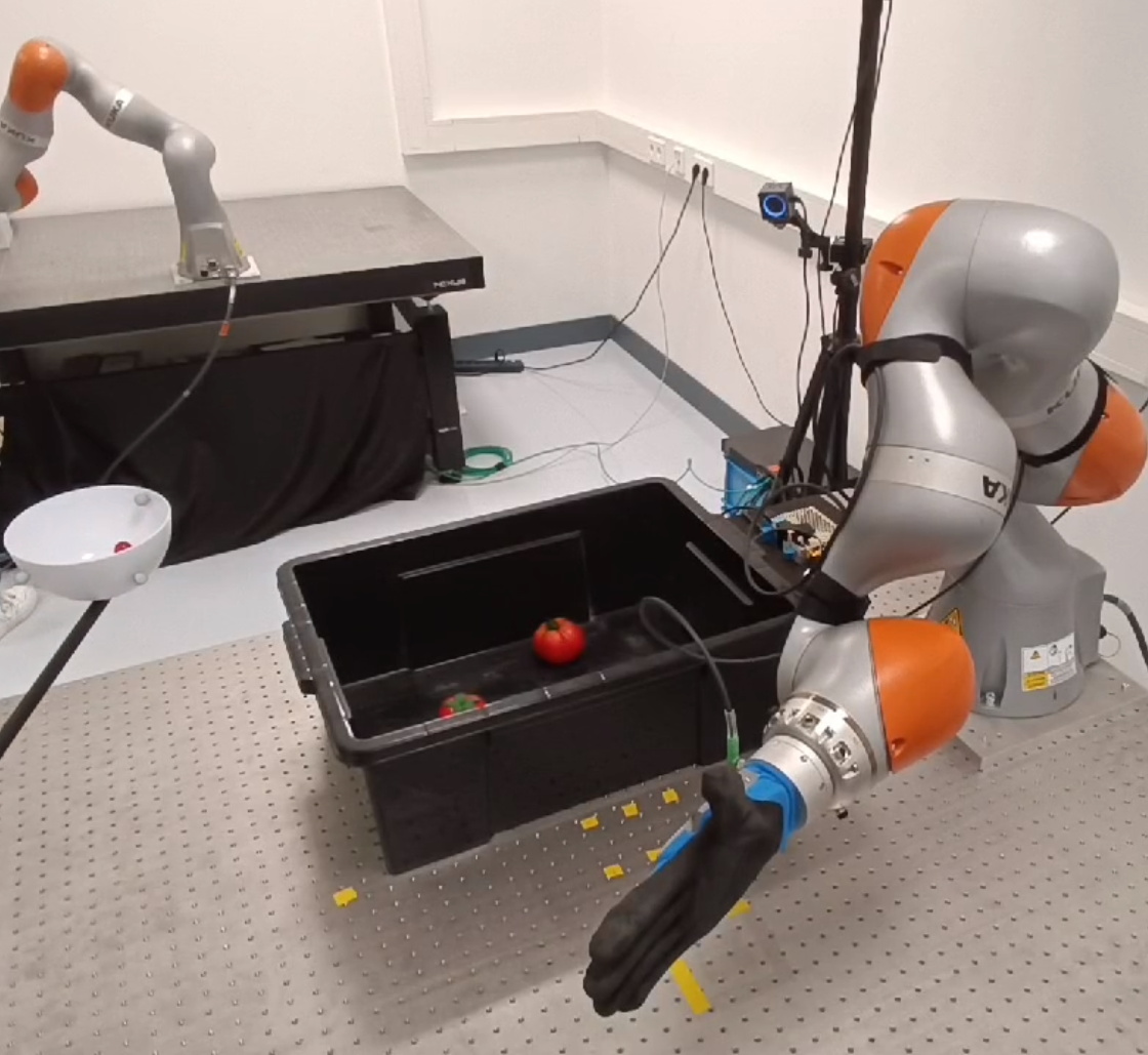
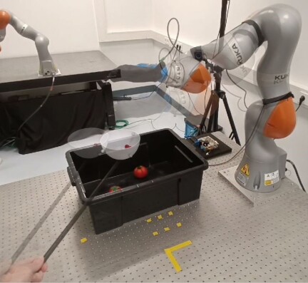
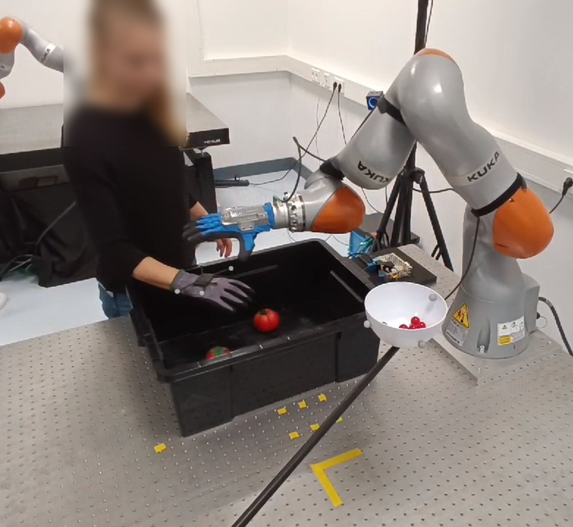
[Initial pose] [Bowl approaches] [Avoid the bowl] [Avoid the hand] [Goal reached]

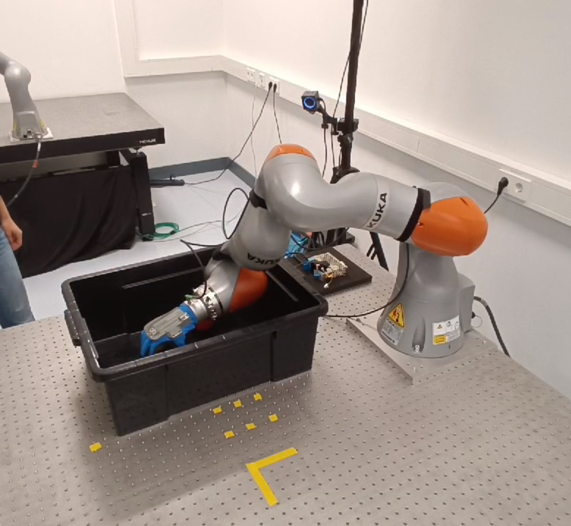
Figure 2: Selected time frames of CPM during a tomato-picking task with the bowl and hand as dynamic obstacles.

[Initial pose] [Avoid the helmet] [Avoid the helmet] [Avoid the helmet] [Goal reached]

Figure 3: Selected time frames of CPM during a pouring task with the yellow helmet as a static obstacle.

[Initial pose] [Move to goal] [Goal reached] [Goal moved] [Goal reached]

Figure 4: Selected time frames of CPM during a pouring task where the goal is changed online by the user.

A low-level joint impedance controller tracks the desired velocities and positions, outputting torque commands. This might decrease tracking performance compared to the simulated experiments, but allows users to push the robot away. If the user is no longer applying force to the robot, the system will converge to the goal pose, as illustrated in the videos in the attached material.

5 Conclusion

Imitation learning via stable motion primitives is a suitable approach for learning motion profiles from demonstrations while providing convergence to the goal. We introduced TamedPUMA, a safe and stable extension of learned stable motion primitives augmented with the recently developed geometric fabrics for safe and stable operations in the presence of obstacles. We proposed two variations, the Forcing Policy Method and Compatible Potential Method, ensuring respectively that the goal is stable, or the stronger notion that the system converges towards the reachable goal. Experiments were carried out both in simulation and in the real world. When trained on a tomato-picking task or pouring task, the proposed TamedPUMA generates a desired motion profile using a DNN while taking whole-body collision avoidance and joint limits into account, with a computation time of just 4-7 $ms$.

This project has received funding from the European Union through ERC, INTERACT, under Grant 101041863, and by the NXTGEN national program. Views and opinions expressed are however those of the authors only and do not necessarily reflect those of the European Union or the NXTGEN national program. Neither the European Union nor the granting authority can be held responsible for them.

References

- Ahn et al. (2023) Kwangjun Ahn, Zakaria Mhammedi, Horia Mania, Zhang-Wei Hong, and Ali Jadbabaie. Model predictive control via on-policy imitation learning. In Learning for Dynamics and Control Conference, pages 1493–1505. PMLR, 2023.
- Bao et al. (2012) David Bao, S-S Chern, and Zhongmin Shen. An introduction to Riemann-Finsler geometry, volume 200. Springer Science & Business Media, 2012.
- Billard et al. (2022) Aude Billard, Sina Mirrazavi, and Nadia Figueroa. Learning for adaptive and reactive robot control: a dynamical systems approach. Mit Press, 2022.
- Bullo and Lewis (2019) Francesco Bullo and Andrew D Lewis. Geometric control of mechanical systems: modeling, analysis, and design for simple mechanical control systems, volume 49. Springer, 2019.
- Coumans and Bai (2016) Erwin Coumans and Yunfei Bai. Pybullet, a python module for physics simulation for games, robotics and machine learning. http://pybullet.org, 2016.
- Fernandez and Billard (2018) NB Figueroa Fernandez and A Billard. A physically-consistent bayesian non-parametric mixture model for dynamical system learning. Proceedings of Machine Learning Research, 2018.
- Ginesi et al. (2019) Michele Ginesi, Daniele Meli, Andrea Calanca, Diego Dall’Alba, Nicola Sansonetto, and Paolo Fiorini. Dynamic movement primitives: Volumetric obstacle avoidance. In 2019 19th international conference on advanced robotics (ICAR), pages 234–239. IEEE, 2019.
- Hewing et al. (2020) Lukas Hewing, Kim P Wabersich, Marcel Menner, and Melanie N Zeilinger. Learning-based model predictive control: Toward safe learning in control. Annual Review of Control, Robotics, and Autonomous Systems, 3:269–296, 2020.
- Hu et al. (2023) Yingbai Hu, Mingyang Cui, Jianghua Duan, Wenjun Liu, Dianye Huang, Alois Knoll, and Guang Chen. Model predictive optimization for imitation learning from demonstrations. Robotics and Autonomous Systems, 163:104381, 2023.
- Hu et al. (2024) Yingbai Hu, Fares J Abu-Dakka, Fei Chen, Xiao Luo, Zheng Li, Alois Knoll, and Weiping Ding. Fusion dynamical systems with machine learning in imitation learning: A comprehensive overview. Information Fusion, page 102379, 2024.
- Huber et al. (2023) Lukas Huber, Jean-Jacques Slotine, and Aude Billard. Avoidance of concave obstacles through rotation of nonlinear dynamics. IEEE Transactions on Robotics, 2023.
- Ijspeert et al. (2013) Auke Jan Ijspeert, Jun Nakanishi, Heiko Hoffmann, Peter Pastor, and Stefan Schaal. Dynamical movement primitives: learning attractor models for motor behaviors. Neural computation, 25(2):328–373, 2013.
- Jaquier et al. (2020) Noémie Jaquier, Leonel Rozo, Sylvain Calinon, and Mathias Bürger. Bayesian optimization meets riemannian manifolds in robot learning. In Conference on Robot Learning, pages 233–246. PMLR, 2020.
- Kaya and Bilge (2019) Mahmut Kaya and Hasan Şakir Bilge. Deep metric learning: A survey. Symmetry, 11(9):1066, 2019.
- Khansari-Zadeh and Billard (2011) S Mohammad Khansari-Zadeh and Aude Billard. Learning stable nonlinear dynamical systems with gaussian mixture models. IEEE Transactions on Robotics, 27(5):943–957, 2011.
- Khansari-Zadeh and Billard (2012) Seyed Mohammad Khansari-Zadeh and Aude Billard. A dynamical system approach to realtime obstacle avoidance. Autonomous Robots, 32:433–454, 2012.
- Khatib (1987) Oussama Khatib. A unified approach for motion and force control of robot manipulators: The operational space formulation. IEEE Journal on Robotics and Automation, 3(1):43–53, 1987.
- Klein et al. (2022) Holger Klein, Noémie Jaquier, Andre Meixner, and Tamim Asfour. A riemannian take on human motion analysis and retargeting. In 2022 IEEE/RSJ International Conference on Intelligent Robots and Systems (IROS), pages 5210–5217. IEEE, 2022.
- Lemme et al. (2014) Andre Lemme, Klaus Neumann, René Felix Reinhart, and Jochen J Steil. Neural learning of vector fields for encoding stable dynamical systems. Neurocomputing, 141:3–14, 2014.
- Li et al. (2023) Ge Li, Zeqi Jin, Michael Volpp, Fabian Otto, Rudolf Lioutikov, and Gerhard Neumann. Prodmp: A unified perspective on dynamic and probabilistic movement primitives. IEEE Robotics and Automation Letters, 8(4):2325–2332, 2023.
- Mohammadi et al. (2024) Hadi Beik Mohammadi, Søren Hauberg, Georgios Arvanitidis, Nadia Figueroa, Gerhard Neumann, and Leonel Rozo. Neural contractive dynamical systems. In The Twelfth International Conference on Learning Representations, 2024.
- Osa et al. (2018) Takayuki Osa, Joni Pajarinen, Gerhard Neumann, J Andrew Bagnell, Pieter Abbeel, Jan Peters, et al. An algorithmic perspective on imitation learning. Foundations and Trends® in Robotics, 7(1-2):1–179, 2018.
- Pérez-Dattari and Kober (2023) Rodrigo Pérez-Dattari and Jens Kober. Stable motion primitives via imitation and contrastive learning. IEEE Transactions on Robotics, 39(5):3909–3928, 2023.
- Pérez-Dattari et al. (2024) Rodrigo Pérez-Dattari, Cosimo Della Santina, and Jens Kober. Puma: Deep metric imitation learning for stable motion primitives. Advanced Intelligent Systems, page 2400144, 2024.
- Perrin and Schlehuber-Caissier (2016) Nicolas Perrin and Philipp Schlehuber-Caissier. Fast diffeomorphic matching to learn globally asymptotically stable nonlinear dynamical systems. Systems & Control Letters, 96:51–59, 2016.
- Pervez et al. (2017) Affan Pervez, Yuecheng Mao, and Dongheui Lee. Learning deep movement primitives using convolutional neural networks. In 2017 IEEE-RAS 17th international conference on humanoid robotics (Humanoids), pages 191–197. IEEE, 2017.
- Przystupa et al. (2023) Michael Przystupa, Faezeh Haghverd, Martin Jagersand, and Samuele Tosatto. Deep probabilistic movement primitives with a bayesian aggregator. In 2023 IEEE/RSJ International Conference on Intelligent Robots and Systems (IROS), pages 3704–3711. IEEE, 2023.
- Rakita et al. (2021) Daniel Rakita, Haochen Shi, Bilge Mutlu, and Michael Gleicher. Collisionik: A per-instant pose optimization method for generating robot motions with environment collision avoidance. In 2021 IEEE International Conference on Robotics and Automation (ICRA), pages 9995–10001. IEEE, 2021.
- Rana et al. (2020) Muhammad Asif Rana, Anqi Li, Dieter Fox, Byron Boots, Fabio Ramos, and Nathan Ratliff. Euclideanizing flows: Diffeomorphic reduction for learning stable dynamical systems. In Learning for Dynamics and Control, pages 630–639. PMLR, 2020.
- Ratliff and Van Wyk (2023) Nathan Ratliff and Karl Van Wyk. Fabrics: A foundationally stable medium for encoding prior experience. arXiv preprint:2309.07368, 2023.
- Ratliff et al. (2018) Nathan D Ratliff, Jan Issac, Daniel Kappler, Stan Birchfield, and Dieter Fox. Riemannian motion policies. arXiv preprint arXiv:1801.02854, 2018.
- Ratliff et al. (2020) Nathan D Ratliff, Karl Van Wyk, Mandy Xie, Anqi Li, and Muhammad Asif Rana. Optimization fabrics. arXiv preprint arXiv:2008.02399, 2020.
- Ridge et al. (2020) Barry Ridge, Andrej Gams, Jun Morimoto, Aleš Ude, et al. Training of deep neural networks for the generation of dynamic movement primitives. Neural Networks, 127:121–131, 2020.
- Saveriano et al. (2023) Matteo Saveriano, Fares J Abu-Dakka, and Ville Kyrki. Learning stable robotic skills on riemannian manifolds. Robotics and Autonomous Systems, 169:104510, 2023.
- Spahn et al. (2023) Max Spahn, Martijn Wisse, and Javier Alonso-Mora. Dynamic optimization fabrics for motion generation. IEEE Transactions on Robotics, 2023.
- Tagliabue and How (2023) Andrea Tagliabue and Jonathan P How. Efficient deep learning of robust policies from mpc using imitation and tube-guided data augmentation. arXiv preprint arXiv:2306.00286, 2023.
- Tedrake (2023) Russ Tedrake. Robotic Manipulation. 2023. URL http://manipulation.mit.edu.
- Ude et al. (2014) Aleš Ude, Bojan Nemec, Tadej Petrić, and Jun Morimoto. Orientation in cartesian space dynamic movement primitives. In 2014 IEEE International Conference on Robotics and Automation (ICRA), pages 2997–3004. IEEE, 2014.
- Urain et al. (2020) J Urain, M Ginesi, D Tateo, and J Peters. Imitationflow: Learning deep stable stochastic dynamic systems by normalizing flows. In RSJ International Conference on Intelligent Robots and Systems (IROS), pages 5231–5237, 2020.
- Van Wyk et al. (2023) Karl Van Wyk, Ankur Handa, Viktor Makoviychuk, Yujie Guo, Arthur Allshire, and Nathan D. Ratliff. Geometric fabrics: a safe guiding medium for policy learning. arXiv preprint arXiv:2310.12831, 2023.
- Xiao et al. (2022) Xuesu Xiao, Tingnan Zhang, Krzysztof Choromanski, Edward Lee, Anthony Francis, Jake Varley, Stephen Tu, Sumeet Singh, Peng Xu, Fei Xia, et al. Learning model predictive controllers with real-time attention for real-world navigation. Proceedings of The 6th Conference on Robot Learning, 205:1708-1721, 2022.
- Xie et al. (2020) Mandy Xie, Karl Van Wyk, Anqi Li, Muhammad Asif Rana, Qian Wan, Dieter Fox, Byron Boots, and Nathan Ratliff. Geometric fabrics for the acceleration-based design of robotic motion. arXiv preprint arXiv:2010.14750, 2020.
- Xie et al. (2021) Mandy Xie, Anqi Li, Karl Van Wyk, Frank Dellaert, Byron Boots, and Nathan Ratliff. Imitation learning via simultaneous optimization of policies and auxiliary trajectories. arXiv preprint arXiv:2105.03019, 2021.
- Xie et al. (2023) Mandy Xie, Ankur Handa, Stephen Tyree, Dieter Fox, Harish Ravichandar, Nathan D Ratliff, and Karl Van Wyk. Neural geometric fabrics: Efficiently learning high-dimensional policies from demonstration. In Conference on Robot Learning, pages 1355–1367. PMLR, 2023.