Likelihood Reward Redistribution

Abstract

In many practical reinforcement learning scenarios, feedback is provided only at the end of a long horizon, leading to sparse and delayed rewards. Existing reward redistribution methods typically assume that per-step rewards are independent, thus overlooking interdependencies among state–action pairs. In this paper, we propose a Likelihood Reward Redistribution (LRR) framework that addresses this issue by modeling each per-step reward with a parametric probability distribution whose parameters depend on the state–action pair. By maximizing the likelihood of the observed episodic return via a leave-one-out (LOO) strategy that leverages the entire trajectory, our framework inherently introduces an uncertainty regularization term into the surrogate objective. Moreover, we show that the conventional mean squared error (MSE) loss for reward redistribution emerges as a special case of our likelihood framework when the uncertainty is fixed under the Gaussian distribution. When integrated with an off-policy algorithm such as Soft Actor-Critic, LRR yields dense and informative reward signals, resulting in superior sample efficiency and policy performance on Box-2d and MuJoCo benchmarks.

1 Introduction

Reinforcement learning (RL) has been successfully applied in a wide range of fields, from fraud detection [7, 3] and advanced manufacturing [11, 5, 13] to autonomous robotics [17, 14, 6] and supply chain optimization [10, 4]. However, a critical challenge remains: in many practical systems, feedback is provided only after a long sequence of actions, rather than immediately. For example, in aerospace design, the quality of an aircraft component is evaluated only after the complete manufacturing process is finished [15]. This delayed feedback creates an extremely sparse reward landscape, making it difficult to determine which actions most significantly influenced the final outcome. Consequently, the learning process may converge slowly or become trapped in suboptimal policies. Recent studies [2, 9, 16, 18] have started to address these issues from different perspectives. Overcoming this bottleneck is essential for developing more robust and efficient RL solutions across diverse application domains.

A widely adopted strategy to tackle sparse rewards is to decompose the episodic return into per-step contributions, thereby generating a dense reward signal. However, conventional return decomposition approaches typically assume that each state’s contribution is independent and depends solely on the current state and action. This Markovian assumption overlooks the interdependencies present in many tasks. Empirical evidence, as summarized in Table 1(a), shows significant lag-1 autocorrelation in several environments, indicating that actions are interdependent over time. Ignoring such dependencies can lead to ineffective credit assignment, where important interactions between actions are missed, ultimately impairing learning efficiency.

To address these issues, we propose a novel reward redistribution framework that explicitly models the interdependent structure of episodic rewards. Instead of treating per-step rewards as isolated signals, our method assumes that each reward is drawn from a pre-specified distribution, with distribution parameters determined by the corresponding state–action pair. By leveraging a leave-one-out (LOO) strategy, our framework computes the likelihood of the observed total return while capturing the interdependencies across the entire trajectory. This probabilistic approach not only distributes credit more coherently over time but also incorporates uncertainty, allowing the model to adjust its confidence in noisy regions.

Our main contributions are summarized as follows:

• We introduce a maximum likelihood framework for reward redistribution that models per-step rewards as random variables and employs a leave-one-out strategy to capture temporal dependencies among state–action pairs.

• We offer theoretical insights demonstrating that our maximum likelihood framework inherently balances prediction accuracy and uncertainty regularization.

• We develop a practical algorithm that integrates our probabilistic reward redistribution approach with Soft Actor-Critic (SAC), demonstrating improved sample efficiency and policy performance on standard benchmarks.

(a) A summary of Lag-1 Autocorrelation ($\rho_{1}$)

Env	$\rho_{1}$	95% CI
BipedalWalker-v3 (BW)	0.30	(0.28, 0.33)
LunarLander-v3 (LL)	-0.13	(-0.16, -0.10)
Ant-v4 (Ant)	0.55	(0.54, 0.57)
HalfCheetah-v4 (HC)	0.54	(0.54, 0.55)
Hopper-v4 (Hop)	0.92	(0.91, 0.93)
Humanoid-v4 (HM)	0.78	(0.75, 0.81)
HumanoidStandup-v4 (HS)	0.97	(0.97, 0.98)
Pusher-v5 (Push)	0.02	(0.01, 0.03)
Reacher-v4 (Reach)	0.01	(0.00, 0.03)
Swimmer-v4 (Swim)	0.91	(0.91, 0.91)
Walker2d-v4 (Walk)	0.88	(0.87, 0.88)

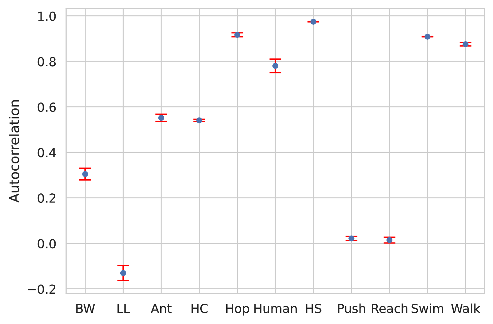
(b) Lag-1 autocorrelation visualization.

Figure 1: Lag-1 reward autocorrelation and its visualization on several Mujoco environments

2 Background

2.1 Reward Redistribution

Traditional reinforcement learning approaches typically assume that the environment can be modeled as a Markov decision process (MDP) characterized by the tuple $\mathcal{M}=\langle\mathcal{S},\mathcal{A},P,R,\mu\rangle$, where $\mathcal{S}$ and $\mathcal{A}$ denote the state and action spaces, $P(s^{\prime}|s,a)$ captures the unknown dynamics, and $R(s,a)$ is the reward function. The initial state distribution is given by $\mu$. The goal is to learn a policy $\pi\colon\mathcal{S}\to\mathcal{A}$ that maximizes the expected discounted sum of rewards:

$$J(\pi)=\mathbb{E}\left[\sum_{t=0}^{\infty}\gamma^{t}\,R(s_{t},\pi(s_{t}))\,\Big{|}\,s_{0}\sim\mu\right],$$

where $\gamma$ is the discount factor. However, many real-world tasks provide feedback only at the end of an episode. Let $\tau=\{s_{0},a_{0},s_{1},\dots,s_{T}\}$ be a trajectory with a cumulative reward $R_{\text{ep}}(\tau)$. In this episodic setting, the objective becomes

$$J_{\text{ep}}(\pi)=\mathbb{E}\left[R_{\text{ep}}(\tau)\,\Big{|}\,\tau\sim\pi\right].$$

Because intermediate rewards are not provided, the decision process loses its strict Markov property. Nonetheless, it is often assumed that the overall return can be approximately decomposed additively as

$$R_{\text{ep}}(\tau)\approx\sum_{t=0}^{T-1}R_{b}(s_{t},a_{t}),$$

where $R_{b}(s,a)$ is an underlying per-step reward function.

To overcome the challenges associated with sparse episodic feedback, reward redistribution techniques aim to derive a surrogate reward function $R_{b}(s,a)$ that transforms the delayed signal into a dense, step-by-step reward. A popular method to achieve this is through return decomposition [1, 8]. In this approach, one trains a parameterized reward model $R_{\theta}(s,a)$ by minimizing the regression loss

$$L_{\text{RD}}(\theta)=\mathbb{E}_{\tau\sim D}\left[\left(R_{\text{ep}}(\tau)-\sum_{t=0}^{T-1}R_{\theta}(s_{t},a_{t})\right)^{2}\right],$$ (1)

where $D$ is the dataset of collected trajectories. By reducing this loss, the model is encouraged to assign local rewards that, when summed over the trajectory, closely match the true episodic return. Once a reliable proxy $R_{\theta}(s,a)$ is obtained, it can be used to replace the sparse terminal reward with a more informative, dense signal, thereby facilitating more effective credit assignment and accelerating policy optimization in environments with delayed rewards.

2.2 Related Works

LIRPG [19] tackles sparse extrinsic rewards by simultaneously learning a policy and an intrinsic reward function. The policy is optimized with respect to a combined reward signal that augments the extrinsic feedback with additional intrinsic rewards, while the intrinsic reward function is updated using meta-gradients to improve the agent’s extrinsic performance. This joint training framework enables the agent to obtain richer learning signals and achieve better performance in tasks with delayed or sparse rewards.
GASIL [12] leverages a generative adversarial framework to encourage an agent to reproduce its own high-return trajectories. It maintains a buffer of past "good" trajectories and trains a discriminator to distinguish these from the agent’s current behavior. The output of the discriminator serves as a learned, dense reward signal, guiding the policy to imitate the best past behaviors even when environmental rewards are sparse or delayed. This adversarial reward shaping can be easily combined with policy gradient methods, improving long-term credit assignment and overall learning efficiency.
RUDDER [2] addresses the challenge of delayed rewards by transforming an episodic, sparse-reward problem into one with dense, immediate rewards. It achieves this by using an LSTM to predict the total return of a trajectory and then decomposing that return into contributions from individual state–action pairs. These contributions serve as redistributed rewards, effectively shifting long-term credit back to the key actions that drive the overall performance. As a result, the method simplifies the credit assignment problem, accelerates learning, and can yield substantial speed-ups in environments where rewards are delayed.
ICRC [9] presents an approach that converts sparse, delayed environmental rewards into dense guidance rewards without the overhead of training extra neural networks. The method works by uniformly smoothing the overall return across all state–action pairs, thereby assigning each pair an equal share of the observed return from past trajectories. This uniform redistribution alleviates the challenges of temporal credit assignment and enhances value estimation, ultimately enabling standard RL algorithms to learn more efficiently even when reward signals are delayed.
RRD [16] addresses the challenges of long-horizon credit assignment by approximating the return decomposition objective via Monte Carlo sampling over short subsequences of a trajectory. Instead of processing every state–action pair along the full trajectory—which is computationally expensive—RRD randomly samples a subset and uses this to estimate the total return. This surrogate loss function includes a variance penalty that regularizes the proxy rewards, effectively bridging between precise return decomposition and uniform reward redistribution. The approach improves scalability and sample efficiency in settings with delayed rewards while preserving the optimal policy.

3 Likelihood Reward Redistribution

In this section, we present a novel reward redistribution framework that leverages probabilistic modeling. Unlike conventional methods that rely on either deterministic regression approaches [1] or subsample segments of trajectories — both of which treat rewards as isolated, Markovian signals, our method models the per-step proxy reward as a random variable and computes the likelihood over the entire trajectory using the leave-one-out (LOO) strategy. This approach integrates the interdependencies between state–action pairs and captures temporal correlations in a holistic manner. Moreover, our formulation inherently incorporates an uncertainty regularizer that robustly mitigates trivial solutions, and we show that the traditional reward redistribution is a special case of our method.

3.1 Gaussian Likelihood

In this section, we start with modeling the reward as a Gaussian random variable, where each state–action pair is assigned both a mean and a standard deviation. By applying a leave-one-out (LOO) strategy, we compute the likelihood over the full trajectory to capture the dependencies between time steps. In Section 3.1.1, we introduce the Gaussian likelihood reward redistribution model and its objective function, while Section 3.1.2 provides a detailed analysis of the method’s properties.

3.1.1 Gaussian Reward Modeling

Suppose the proxy reward for each state-action pair $(s,a)$ follows a Gaussian random variable, i.e.,

$$r_{\theta}(s,a)\sim\mathcal{N}\big{(}\mu_{\theta}(s,a),\sigma_{\theta}(s,a)^{2}\big{)},$$

where $\mu_{\theta}(s,a)$ and $\sigma_{\theta}(s,a)>0$ are parameterized by a neural network with parameter $\theta$. Consequently, the conditional density can be written as

$$P\bigl{(}r|s,a;\theta\bigr{)}=\frac{1}{\sqrt{2\pi}\,\sigma_{\theta}(s,a)}\exp\!\left(-\frac{(r-\mu_{\theta}(s,a))^{2}}{2\sigma_{\theta}(s,a)^{2}}\right).$$ (2)

Given a trajectory $\tau=\{(s_{0},a_{0}),\dots,(s_{T-1},a_{T-1})\}$ and the corresponding episodic reward $R_{\mathrm{ep}}(\tau)$ provided by the environment, the reward proxy model outputs the parameters $\mu_{\theta}(s_{t},a_{t})$ and $\sigma_{\theta}(s_{t},a_{t})$ at each time step $t$. In order to consider the interdependence among state–action pairs, we adopted a leave-one-out strategy. Specifically, for each time step $i$, the rewards for all $t\neq i$ are generated by $\hat{r}(s_{t},a_{t})=\mu_{\theta}(s_{t},a_{t})+\epsilon\,\sigma_{\theta}(s_{t},a_{t})$, which leads to the leave-one-out predicted reward $\tilde{r}(s_{i},a_{i})$ as

$$\tilde{r}(s_{i},a_{i})=R_{\mathrm{ep}}(\tau)-\sum_{t=0,\,t\neq i}^{T-1}\hat{r}(s_{t},a_{t}).$$

Following Eq (2), the negative log-likelihood for such a prediction is then given by

$$\ell_{i}(\theta)=\log\sigma_{\theta}(s_{i},a_{i})+\frac{\bigl{(}\tilde{r}(s_{i},a_{i})-\mu_{\theta}(s_{i},a_{i})\bigr{)}^{2}}{2\,\sigma_{\theta}(s_{i},a_{i})^{2}}.$$ (3)

Then the overall objective function is defined by

$$\mathcal{L}(\theta)=\mathbb{E}_{\tau\sim\mathcal{D}}\big{[}\ell(\tau;\theta)\big{]},$$ (4)

where $\ell(\tau;\theta)$ is the loss function for the whole trajectory which is $\ell(\tau;\theta)=\frac{1}{|\tau|}\sum_{i=0}^{|\tau|-1}\ell_{i}(\theta)$ and $|\tau|$ is the length of the trajectory.

3.1.2 Analysis of Gaussian Reward Redistribution

Define the soft reward redistribution function under parameter $\theta$ along the trajectory $\tau$ as

$$\ell_{\mathrm{RR}}(\tau;\theta)=R_{\mathrm{ep}}(\tau)-\sum_{t=0}^{T-1}\mu_{\theta}(s_{t},a_{t}).$$ (5)

Then the predicted reward of a specific pair $(s_{i},a_{i})$ on the trajectory is

$$\tilde{r}(s_{i},a_{i};\theta) =R_{\text{ep}}(\tau)-\sum_{t=0,\,t\neq i}^{|\tau|-1}\hat{r}(s_{t},a_{t};\theta)$$

$$=\ell_{\mathrm{RR}}(\tau;\theta)+\mu_{\theta}(s_{i},a_{i})-\sum_{t=0,\,t\neq i}^{|\tau|-1}\epsilon_{t}\cdot\sigma_{\theta}(s_{t},a_{t}).$$ (6)

Substituting into the per-step negative log-likelihood loss (3), we obtain that

$$\ell_{i}(\theta)=\log\sigma_{\theta}(s_{i},a_{i})+\frac{\Bigl{(}\ell_{\mathrm{RD}}(\tau;\theta)-\sum_{t=0,\,t\neq i}^{|\tau|-1}\epsilon_{t}\cdot\sigma_{\theta}(s_{t},a_{t})\Bigr{)}^{2}}{2\,\sigma_{\theta}(s_{i},a_{i})^{2}},$$

then the overall negative log-likelihood becomes

$$L(\theta)=\mathbb{E}_{\tau\sim D}\!\left[\frac{1}{T}\sum_{i=0}^{T-1}\left\{\log\sigma_{\theta}(s_{i},a_{i})+\frac{\Bigl{(}\ell_{\mathrm{RD}}(\tau;\theta)-\sum_{t=0,\,t\neq i}^{|\tau|-1}\epsilon_{t}\cdot\sigma_{\theta}(s_{t},a_{t})\Bigr{)}^{2}}{2\,\sigma_{\theta}(s_{i},a_{i})^{2}}\right\}\right].$$

Proposition 1 (Special Case).

If $\sigma_{\theta}(s_{t},a_{t})=1$ for all $(s_{t},a_{t})$ and no noise is introduced during training, then the likelihood reward redistribution reduces to the original reward redistribution (1).

Proposition 2 (Optimal Trade-off between Accuracy and Uncertainty).

For any state–action pair $(s_{i},a_{i})$ with per-step negative log-likelihood loss $\ell_{i}(\theta)$ given by (3), and defining $\delta_{i}=\tilde{r}(s_{i},a_{i})-\mu_{\theta}(s_{i},a_{i})$, the loss $\ell_{i}(\theta)$ is minimized if and only if $\sigma_{\theta}(s_{i},a_{i})=|\delta_{i}|$.

Proof.

Define $f(\sigma)=\log\sigma+\frac{\delta_{i}^{2}}{2\sigma^{2}}\,(\sigma>0)$, with $f^{\prime}(\sigma)=\frac{1}{\sigma}\left(1-\frac{\delta_{i}^{2}}{\sigma^{2}}\right)$. Setting $f^{\prime}(\sigma)=0$ gives $\sigma=|\delta_{i}|$. Moreover, since $f^{\prime\prime}(\sigma)=-\frac{1}{\sigma^{2}}+\frac{3\delta_{i}^{2}}{\sigma^{4}}$, and at $\sigma=|\delta_{i}|$, $f^{\prime\prime}(|\delta_{i}|)=\frac{2}{\delta_{i}^{2}}>0$. ∎

Remark 1.

The proposition 2 shows that the per-step loss is minimized when

$$\sigma_{\theta}(s,a)=|\tilde{r}(s,a)-\mu_{\theta}(s,a)|,$$

which means the loss naturally balances accuracy and uncertainty. To further interpret this effect, reparameterize the uncertainty as

$$\sigma_{\theta}(s,a)=\alpha\,|\tilde{r}(s,a)-\mu_{\theta}(s,a)|.$$

The loss then becomes

$$L(\alpha)=\log\bigl{(}\alpha\,|\tilde{r}(s,a)-\mu_{\theta}(s,a)|\bigr{)}+\frac{1}{2\alpha^{2}},$$

which is minimized at $\alpha=1$. This shows that any deviation from the optimal balance increases the loss, effectively serving as an implicit regularizer. In regions with small prediction error, enforcing a low $\sigma_{\theta}(s,a)$ amplifies the weight on the error term, promoting precise fitting. Conversely, in noisy regions, a larger $\sigma_{\theta}(s,a)$ down-weights the error, helping to prevent overfitting.

Proposition 3 (Gradient Dynamics for Gaussian).

Recall the per-step negative log-likelihood loss (3)

$$\ell(s,a;\theta)=\log\sigma_{\theta}(s,a)+\frac{\bigl{(}\tilde{r}(s,a)-\mu_{\theta}(s,a)\bigr{)}^{2}}{2\,\sigma_{\theta}(s,a)^{2}},$$

the gradients with respect to the parameter functions are approximately given by

$$\frac{\partial\ell(s,a;\theta)}{\partial\mu_{\theta}(s,a)}\propto\frac{\mu_{\theta}(s,a)-\tilde{r}(s,a)}{\sigma_{\theta}(s,a)^{2}},$$

and

$$\frac{\partial\ell(s,a;\theta)}{\partial\sigma_{\theta}(s,a)}\propto\frac{\sigma_{\theta}(s,a)^{2}-\bigl{(}\tilde{r}(s,a)-\mu_{\theta}(s,a)\bigr{)}^{2}}{\sigma_{\theta}(s,a)^{3}}.$$

Remark 2 (Accuracy Update).

The Proposition 3 reveal that when the uncertainty $\sigma_{\theta}(s,a)$ is small, the gradient magnitude for $\mu_{\theta}(s,a)$ becomes large, leading to more aggressive updates. Conversely, higher uncertainty yields a smaller gradient, which tempers the updates in noisy or uncertain regions.

Remark 3 (Uncertainty Update).

The gradient update with respect to $\sigma_{\theta}(s,a)$ drives the uncertainty estimate toward the absolute prediction error $|\tilde{r}(s,a)-\mu_{\theta}(s,a)|$. That is, when the prediction error is large but the current uncertainty estimate is small, the gradient increases $\sigma_{\theta}(s,a)$ to better capture the noise level; conversely, if the prediction error is small while $\sigma_{\theta}(s,a)$ is overestimated, the gradient decreases it to avoid exaggerating the noise.

3.2 Skew Normal Likelihood

To capture asymmetric reward distributions observed in real-world applications, we extend our framework to use a Skew Normal likelihood. For example, in financial markets, a state–action pair may yield moderate returns most of the time but occasionally experience extreme gains or losses, resulting in a skewed distribution. This extension also highlights the flexibility of our approach, as it can be adapted to incorporate various probability distributions to better model the underlying data.

3.2.1 Skew Normal Reward Modeling

Suppose we model the proxy reward $r_{\theta}(s,a)$ using a Skew Normal distribution with three parameters: the location $\mu_{\theta}(s,a)$, the scale $\sigma_{\theta}(s,a)>0$, and the shape $\lambda_{\theta}(s,a)$, all parameterized by a neural network. The density function is given by

$$P(r|s,a;\theta)=\frac{2}{\sigma_{\theta}(s,a)}\,\phi\!\left(\frac{r-\mu_{\theta}(s,a)}{\sigma_{\theta}(s,a)}\right)\,\Phi\!\left(\lambda_{\theta}(s,a)\,\frac{r-\mu_{\theta}(s,a)}{\sigma_{\theta}(s,a)}\right),$$ (7)

where $\phi(z)$ is the standard normal density and $\Phi(z)$ its cumulative distribution function. Consequently, the per-step negative log-likelihood becomes

$$\ell_{i}(\theta)=\log\sigma_{\theta}(s_{i},a_{i})-\log\phi(z_{i})-\log\Phi\!\Bigl{(}\lambda_{\theta}(s_{i},a_{i})\,z_{i}\Bigr{)}+\text{const},$$ (8)

with $z_{i}=\frac{\tilde{r}(s_{i},a_{i})-\mu_{\theta}(s_{i},a_{i})}{\sigma_{\theta}(s_{i},a_{i})}$. The overall loss for the trajectory is defined analogously to (4).

3.2.2 Analysis of Skew Normal Reward Redistribution

In the Skew Normal framework, the additional shape parameter $\lambda_{\theta}(s,a)$ allows us to capture asymmetries in the reward distribution that the Gaussian model cannot. This extra flexibility not only improves the expressive power of the model but also impacts regularization and gradient dynamics by penalizing over- and underestimation differently.

Proposition 4.

Consider the Skew Normal per-step loss (without constant) given by

$$\ell(\sigma)=\log\sigma+\frac{\delta^{2}}{2\sigma^{2}}-\log\Phi\!\Bigl{(}\lambda\,\frac{\delta}{\sigma}\Bigr{)},$$

where $\delta=\tilde{r}(s,a)-\mu_{\theta}(s,a)$, $\sigma=\sigma_{\theta}(s,a)>0$, $\lambda=\lambda_{\theta}(s,a)$. Then the loss is minimized with respect to $\sigma$ when the optimal scale satisfies

$$\sigma^{*}=\delta\,\frac{-\lambda\,\gamma+\sqrt{(\lambda\,\gamma)^{2}+4}}{2},\quad\text{with}\quad\gamma=\frac{\phi\!\Bigl{(}\lambda\,\frac{\delta}{\sigma^{*}}\Bigr{)}}{\Phi\!\Bigl{(}\lambda\,\frac{\delta}{\sigma^{*}}\Bigr{)}}.$$

In particular, when $\lambda=0$ (the Gaussian case) we have $\sigma^{*}=\delta$.

Remark 4.

A closer examination of Proposition 4 reveals that the additional shape parameter $\lambda$ significantly influences the optimal scale. Specifically, when $\lambda>0$, the optimal $\sigma^{*}$ is less than $\delta$, thereby imposing a stronger penalty on overestimations. Conversely, when $\lambda<0$, $\sigma^{*}$ exceeds $\delta$, which reduces the penalty on underestimations. This asymmetric effect acts as an implicit regularizer, ensuring that the uncertainty estimate adapts appropriately to the skewness present in the reward distribution.

Proposition 5 (Skew-adjusted Gradient Dynamics).

Let $\delta=\tilde{r}(s,a)-\mu_{\theta}(s,a)$. Then the gradients of Skew Normal per-step loss (8) w.r.t $\mu_{\theta}(s,a)$ and $\sigma_{\theta}(s,a)$ are given by

$$\frac{\partial\ell}{\partial\mu_{\theta}(s,a)}\propto-\frac{\delta}{\sigma_{\theta}(s,a)^{2}}+\frac{\lambda_{\theta}(s,a)}{\sigma_{\theta}(s,a)}\,\gamma,$$

and

$$\frac{\partial\ell}{\partial\sigma_{\theta}(s,a)}\propto\frac{1}{\sigma_{\theta}(s,a)}-\frac{\delta^{2}}{\sigma_{\theta}(s,a)^{3}}+\frac{\lambda_{\theta}(s,a)\,\delta}{\sigma_{\theta}(s,a)^{2}}\,\gamma,$$

where $\gamma=\tfrac{\phi\!\Bigl{(}\lambda_{\theta}(s,a)\,\frac{\delta}{\sigma_{\theta}(s,a)}\Bigr{)}}{\Phi\!\Bigl{(}\lambda_{\theta}(s,a)\,\frac{\delta}{\sigma_{\theta}(s,a)}\Bigr{)}}$.

Remark 5.

Compared to the Gaussian case, the Skew Normal model has extra terms $\frac{\lambda_{\theta}(s,a)}{\sigma_{\theta}(s,a)}\,\gamma$ for $\mu_{\theta}(s,a)$ and $\frac{\lambda_{\theta}(s,a)\,\delta}{\sigma_{\theta}(s,a)^{2}}\,\gamma$ for $\sigma_{\theta}(s,a)$. When $\delta>0$ (indicating that the predicted mean is too low), a positive $\lambda_{\theta}(s,a)$ dampens the updates, thereby reducing overcorrection. Conversely, when $\delta<0$ (indicating that the prediction is too high), a negative $\lambda_{\theta}(s,a)$ amplifies the updates, enforcing a stronger correction. This asymmetric adjustment helps the model better capture and adapt to skewed reward distributions.

3.3 Practical Implementation of Gaussian Reward Redistribution

In this section, we introduce the practical algorithm for Gaussian reward redistribution (Algorithm 1). Note that our framework can be readily extended to other probability distributions by replacing Equation (9) with the corresponding sampling procedure and Equation (10) with its log-likelihood function. For a given trajectory $\tau=\{(s_{0},a_{0}),\ldots,(s_{T-1},a_{T-1})\}$ with episodic reward $R_{\mathrm{ep}}(\tau)$, a leave-one-out return is computed at each time step by excluding that step’s contribution from the total reward. The per-step loss is defined as the Gaussian negative log-likelihood, and the overall loss is the average over all time steps.

Algorithm 1 Gaussian Likelihood Reward Redistribution

1:Input: Reward model parameters $\theta$, learning rate $\alpha$, update iterations $N$, mini-batch size $M$

2:Initialize replay buffer $D\leftarrow\emptyset$

3:while training not converged do

4:  Collect a rollout trajectory $\tau=\{(s_{0},a_{0}),\ldots,(s_{T-1},a_{T-1})\}$ and episodic reward $R_{\mathrm{ep}}(\tau)$

5:  Store $(\tau,R_{\mathrm{ep}}(\tau))$ in $D$

6:  for $k=1$ to $N$ do

7:   Sample a mini-batch $\{(\tau_{j},R_{\mathrm{ep}}(\tau_{j}))\}_{j=1}^{M}$ from $D$

8:   for each trajectory $\tau_{j}=\{(s_{0}^{j},a_{0}^{j}),\ldots,(s_{|\tau_{j}|-1}^{j},a_{|\tau_{j}|-1}^{j})\}$ do

9:     for $i\in\{|\tau_{j}|\}$ (in parallel) do

10:      Sample independent noise $\epsilon_{i,t}^{j}\sim\mathcal{N}(0,1)$

11:      Compute leave-one-out return

$$\tilde{r}(s_{i}^{j},a_{i}^{j})=\sum_{t\neq i}\left(\mu_{\theta}(s_{t}^{j},a_{t}^{j})+\sigma_{\theta}(s_{t}^{j},a_{t}^{j})\epsilon_{i,t}^{j}\right)$$ (9)

12:      Compute individual loss

$$\ell_{i}^{j}(\theta)=\log\sigma_{\theta}(s_{i}^{j},a_{i}^{j})+\frac{\bigl{(}\tilde{r}(s_{i}^{j},a_{i}^{j})-\mu_{\theta}(s_{i}^{j},a_{i}^{j})\bigr{)}^{2}}{2\,\sigma_{\theta}(s_{i}^{j},a_{i}^{j})^{2}}$$ (10)

13:     end for

14:     Compute trajectory loss $L(\tau_{j};\theta)=\frac{1}{|\tau_{j}|}\sum_{i=0}^{|\tau_{j}|-1}\ell_{i}^{j}(\theta)$

15:   end for

16:   Compute mini-batch loss: $L(\theta)=\frac{1}{M}\sum_{j=1}^{M}L(\tau_{j};\theta)$

17:   Update $\theta\leftarrow\theta-\alpha\,\nabla_{\theta}L(\theta)$

18:  end for

19:end while

4 Experiments

In this section, we evaluate our proposed Gaussian Reward Redistribution (GRR) method on several Box-2d and MuJoCo locomotion tasks with episodic rewards. As our sole baseline, we use randomized return decomposition (RRD) [16], since the RRD paper already compares with other methods (e.g., ICRC, RUDDER). In our experiments, RRD is configured with a sampling parameter $K=64$ and a task horizon of 1000.

4.1 Experimental Setup

We perform experiments on six Box-2d and MuJoCo tasks: BipedalWalker, HalfCheetah, Hopper, Humanoid, Swimmer, and Walker. In these tasks, the original dense rewards are replaced by episodic rewards, where the agent receives a reward of zero at non-terminal steps and the episodic reward $R_{\mathrm{ep}}(\tau)$ is computed as the sum of per-step rewards and delivered only at the episode end. Our GRR method leverages a probabilistic reward model that predicts both the mean $\mu_{\theta}(s,a)$ and the standard deviation $\sigma_{\theta}(s,a)$ for each state–action pair. A leave-one-out scheme is used to compute a surrogate Gaussian negative log-likelihood loss over full trajectories. Policy optimization is performed using Soft Actor-Critic (SAC) with the default hyper-parameter configuration (see Table 1).

Table 1: Hyper-parameter configuration in MuJoCo and Box-2d environments.

Hyper-Parameter	Default Configuration
Learning rate	$3\times 10^{-4}$
Optimizer (all losses)	Adam (Kingma & Ba, 2015)
Discount factor $\gamma$	0.99
Polyak-averaging coefficient	0.005
Initial temperature $\alpha_{\text{init}}$	1.0
Target entropy	$-\mathrm{dim}(A)$
Activation	ReLU
# hidden layers (all networks)	2
# neurons per layer	256
# gradient steps per environment step	1
# gradient steps per target update	1
# transitions in replay buffer	$10^{5}$
# transitions in mini-batch for training SAC	512
# transitions in mini-batch for training $R_{b}^{\theta}$	4

4.2 Results

Figure 2 summarizes the average episodic returns achieved by GRR (ours) and RRD (baseline) across the six tasks. Our GRR method consistently outperforms RRD, demonstrating improved sample efficiency and final performance.

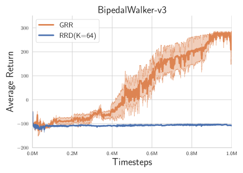
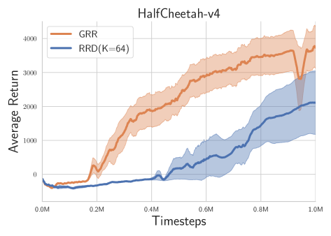
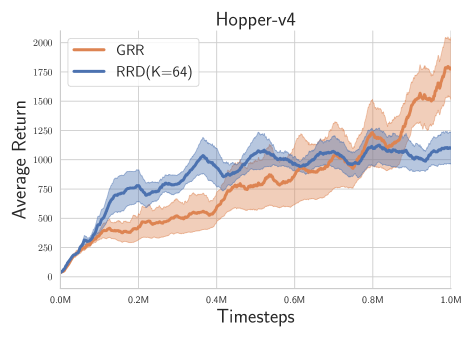
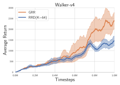
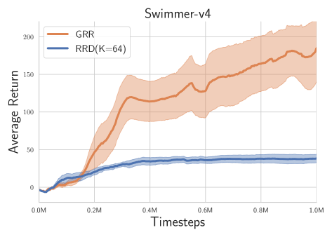
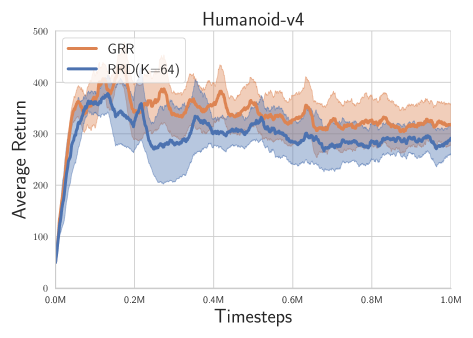
Figure 2: Experimental results on Box-2d and MuJoCo tasks with high reward autocorrelation.

Overall Performance.

As shown in Figure 2, our Gaussian Reward Redistribution (GRR) consistently outperforms the randomized return decomposition (RRD) baseline on the majority of MuJoCo tasks. In environments such as Hopper-v4, Humanoid-v4, and Walker-v4, which exhibit high lag-1 autocorrelation (above 0.8), GRR achieves markedly higher sample efficiency and final performance. We attribute these gains to GRR’s explicit modeling of the non-Markovian structure—i.e., it leverages the correlations among consecutive state–action pairs to allocate credit more coherently. By contrast, RRD relies on randomly sampled subsequences and assumes (in practice) near-independence among them, making it less effective in capturing long-range temporal dependencies.

Influence of Temporal Correlations.

Our experiments show that GRR’s probabilistic framework significantly improves performance in environments with moderate to high lag-1 autocorrelations (e.g., BipedalWalker-v3 and HalfCheetah-v4), supporting the hypothesis that stronger interdependencies among state–action pairs allow the leave-one-out likelihood modeling to better capture temporal structure. Although we did not further test cases with minimal temporal correlation, our analysis suggests that in such settings—where inter-step dependencies are weak—simpler Markovian approaches may perform comparably.

Overall, these results confirm that GRR’s core strength lies in handling non-Markovian tasks, where high lag-1 autocorrelation reveals strong interdependencies across time steps. By modeling each per-step reward with a flexible likelihood and employing a leave-one-out strategy, GRR can more effectively redistribute delayed rewards, leading to superior policy learning in environments with substantial temporal correlations.

5 Conclusion

We have presented a likelihood-based framework for reward redistribution in episodic reinforcement learning, where each per-step reward is modeled by a parametric distribution and optimized via a leave-one-out (LOO) strategy. By incorporating the interdependencies among state–action pairs, our approach effectively addresses non-Markovian reward structures that arise in long-horizon tasks. Theoretical analysis shows that our objective can be decomposed into a conventional return decomposition loss plus a natural uncertainty regularization term; notably, the classical mean-squared-error loss emerges as a special case when uncertainty is held fixed. Empirical results on MuJoCo benchmarks demonstrate that, when combined with Soft Actor-Critic, our method yields dense, robust reward signals that improve both sample efficiency and final policy performance. In future work, we plan to extend this framework to non-Gaussian noise models, explore multi-agent scenarios, and investigate deeper integrations with other off-policy algorithms.

References

- [1] Jose Arjona-Medina et al. Rudder: Return decomposition for delayed rewards. In Advances in Neural Information Processing Systems, 2019.
- [2] Jose A Arjona-Medina, Michael Gillhofer, Michael Widrich, Thomas Unterthiner, Johannes Brandstetter, and Sepp Hochreiter. Rudder: Return decomposition for delayed rewards. Advances in Neural Information Processing Systems, 32, 2019.
- [3] Shi Bo and Minheng Xiao. Data-driven risk measurement by sv-garch-evt model. In 2024 6th International Conference on Data-driven Optimization of Complex Systems (DOCS), pages 849–856. IEEE, 2024.
- [4] Shi Bo and Minheng Xiao. Root cause attribution of delivery risks via causal discovery with reinforcement learning. Algorithms, 17(11):498, 2024.
- [5] Jin Cao, Yanhui Jiang, Chang Yu, Feiwei Qin, and Zekun Jiang. Rough set improved therapy-based metaverse assisting system. In 2024 IEEE International Conference on Metaverse Computing, Networking, and Applications (MetaCom), pages 358–364. IEEE, 2024.
- [6] Jin Cao, Ran Xu, Xinnan Lin, Feiwei Qin, Yong Peng, and Yanli Shao. Adaptive receptive field u-shaped temporal convolutional network for vulgar action segmentation. Neural Computing and Applications, 35(13):9593–9606, 2023.
- [7] Yuxin Dong, Jianhua Yao, Jiajing Wang, Yingbin Liang, Shuhan Liao, and Minheng Xiao. Dynamic fraud detection: Integrating reinforcement learning into graph neural networks. In 2024 6th International Conference on Data-driven Optimization of Complex Systems (DOCS), pages 818–823. IEEE, 2024.
- [8] Yonathan Efroni et al. Return decomposition for delayed rewards. In Proceedings of the AAAI Conference on Artificial Intelligence, 2021.
- [9] Tanmay Gangwani, Yuan Zhou, and Jian Peng. Learning guidance rewards with trajectory-space smoothing. Advances in Neural Information Processing Systems, 33:822–832, 2020.
- [10] Ilaria Giannoccaro. Centralized vs. decentralized supply chains: The importance of decision maker’s cognitive ability and resistance to change. Industrial Marketing Management, 73:59–69, 2018.
- [11] Fatemeh Golpayegani, Saeedeh Ghanadbashi, and Akram Zarchini. Advancing sustainable manufacturing: Reinforcement learning with adaptive reward machine using an ontology-based approach. Sustainability, 16(14):5873, 2024.
- [12] Yijie Guo, Junhyuk Oh, Satinder Singh, and Honglak Lee. Generative adversarial self-imitation learning. arXiv preprint arXiv:1812.00950, 2018.
- [13] Haowei Jiang, Feiwei Qin, Jin Cao, Yong Peng, and Yanli Shao. Recurrent neural network from adder’s perspective: Carry-lookahead rnn. Neural Networks, 144:297–306, 2021.
- [14] Fengming Li, Qi Jiang, Sisi Zhang, Meng Wei, and Rui Song. Robot skill acquisition in assembly process using deep reinforcement learning. Neurocomputing, 345:92–102, 2019.
- [15] Pouria Razzaghi, Amin Tabrizian, Wei Guo, Shulu Chen, Abenezer Taye, Ellis Thompson, Alexis Bregeon, Ali Baheri, and Peng Wei. A survey on reinforcement learning in aviation applications. Engineering Applications of Artificial Intelligence, 136:108911, 2024.
- [16] Zhizhou Ren, Ruihan Guo, Yuan Zhou, and Jian Peng. Learning long-term reward redistribution via randomized return decomposition. arXiv preprint arXiv:2111.13485, 2021.
- [17] Zixiang Wang, Hao Yan, Changsong Wei, Junyu Wang, Shi Bo, and Minheng Xiao. Research on autonomous driving decision-making strategies based deep reinforcement learning. In Proceedings of the 2024 4th International Conference on Internet of Things and Machine Learning, pages 211–215, 2024.
- [18] Minheng Xiao, Xian Yu, and Lei Ying. Policy gradient methods for risk-sensitive distributional reinforcement learning with provable convergence. arXiv preprint arXiv:2405.14749, 2024.
- [19] Zeyu Zheng, Junhyuk Oh, and Satinder Singh. On learning intrinsic rewards for policy gradient methods. Advances in neural information processing systems, 31, 2018.