A Thorough Assessment of the Non-IID Data Impact in Federated Learning

Abstract

Federated learning (FL) allows collaborative machine learning (ML) model training among decentralized clients’ information, ensuring data privacy. The decentralized nature of FL deals with non-independent and identically distributed (non-IID) data. This open problem has notable consequences, such as decreased model performance and larger convergence times. Despite its importance, experimental studies systematically addressing all types of data heterogeneity (a.k.a. non-IIDness) remain scarce. This paper aims to fill this gap by assessing and quantifying the non-IID effect through a thorough empirical analysis. We use the Hellinger Distance (HD) to measure differences in distribution among clients. Our study benchmarks five state-of-the-art strategies for handling non-IID data, including label, feature, quantity, and spatiotemporal skewness, under realistic and controlled conditions. This is the first comprehensive analysis of the spatiotemporal skew effect in FL. Our findings highlight the significant impact of label and spatiotemporal skew non-IID types on FL model performance, with notable performance drops occurring at specific HD thresholds. Additionally, the FL performance is heavily affected mainly when the non-IIDness is extreme. Thus, we provide recommendations for FL research to tackle data heterogeneity effectively. Our work represents the most extensive examination of non-IIDness in FL, offering a robust foundation for future research.

I Introduction

In today’s digital age, the interaction of machine learning (ML) and healthcare or financial data holds immense promise for improving disease diagnosis [36] and combating financial crimes [35]. However, it raises critical questions about data privacy when dealing with sensitive information from hospitals or banks. In this context, trusted research environments emerge as a mechanism for balancing ML research and protecting individual privacy [13].

Federated learning (FL) [30] has emerged as a transformative approach for training ML models across decentralized data sources, preserving data privacy and security. However, a significant challenge inherent in FL is the variation in data distributions across clients referred to as non-IID (Non-Independent and Identically Distributed) data. This so-called non-IIDness hinders model performance and convergence during training [44].

Motivation.

Despite the growing body of research focusing on the challenges posed by non-IID data in FL, there remains a gap in experimental studies that systematically evaluate the effectiveness of FL algorithms under different types of data heterogeneity. Understanding the extent and nature of non-IID characteristics are crucial for developing robust, fair, and widely applicable FL algorithms. In this context, our study uses the Hellinger Distance (HD) [12] to quantify the differences in client data distributions. This approach ensures that our conclusions are robust and generalizable across diverse scenarios.

Contribution.

The subsequent points encapsulate the contributions of our study:

1. We benchmark five of the most employed state-of-the-art aggregation and client selection of FL algorithms to tackle non-IID data distributions among clients under realistic, controlled, and quantifiable methods for synthetic partitioning and all non-IID types (label, feature, quantity, and spatiotemporal skewness). This is the first study thoroughly analyzing how the spatiotemporal skew affects the performance of FL models.

2. We motivate using HD to quantify the differences among data distributions, standardizing the guidelines for systematic studies of data heterogeneity in FL. This is the first work to demonstrate that the effect of the non-IIDness is not the same under all the levels of heterogeneity We use HD to quantify differences in distribution as it provides more granular information, and we leave as future work the exploration of other measures; see our section on design insights and opportunities.

3. We provide a reference to researchers about which methods are robust to which kind of non-IIDness on highly benchmarked datasets.

4. We give highlights and relevant recommendations for FL researchers based on quantifying non-IIDness.

To the best of our knowledge, this is the most comprehensive and complete study of non-IIDness and its effects on FL models.

II Related Work

Studies that analyze and benchmark the performance of methods to tackle the non-IIDness effect on the FL models under controlled and systematic scenarios are scarce. Nevertheless, in this section, we introduce those works that, to some extent, provide empirical analysis about the data heterogeneity repercussions.

A study by Vahidian et al. [43] challenges conventional thinking regarding data heterogeneity in FL. They posit that dissimilar data among participants is not always detrimental and can be advantageous, and we found similar results. Their argument centers on two main points: firstly, that differences in labels (label skew) are not the sole determinant of data heterogeneity, and secondly, that a more effective measure of heterogeneity is the angle between the data subspaces of participating clients. Conversely, we encompass a broader spectrum of non-IIDness types and include images and tabular data.

Wong et al. [45] conduct extensive experiments on a large network of IoT and edge devices to present FL real-world characteristics, including learning performance and operation (computation and communication) costs. Moreover, they mainly concentrate on heterogeneous scenarios, which is the most challenging issue of FL. Although they thoroughly analyze the impact of non-IIDness, they focus on image datasets and do not compare any aggregation method to solve the effects of highly heterogeneous scenarios. Contrarily, this work includes diverse datasets and benchmark state-of-the-art methodologies to handle non-IIDness in FL.

In their study, Mora et al. [31] examine existing solutions in the literature to mitigate the challenges posed by non-IID data. On the one hand, they emphasize the underlying rationale behind these alternative strategies and discuss their potential limitations. Ultimately, they identify the most promising approaches based on empirical results and critical defining characteristics, such as any assumptions made by each strategy. In parallel, they focus only on label skew and only consider one dataset in their experiments. In our paper, we alternatively analyze broader datasets and data skewness types, identifying broader limitations and potential approaches to overcome them.

Wong et al. [45] present a comprehensive analysis of FL characteristics in real-world environments, focusing on large networks of IoT and edge devices. Their work offers valuable insights into learning performance and operational costs, particularly in heterogeneous scenarios. While they provide a detailed exploration of non-IID data issues using image datasets, they do not extensively evaluate different aggregation methods to address highly heterogeneous scenarios. In contrast, our work broadens this scope by incorporating diverse datasets and benchmarking state-of-the-art methods specifically designed to tackle non-IID challenges in FL.

One of the novelties of our study is the use of metrics to quantify non-IIDness among clients. The latter facilitates the systematic and regulated selection of non-IID. To the best of our knowledge, our work is the first to employ these metrics in the relevant bibliography.

III Background

III-A Federated learning basics

FL [30] is particularly suited for scenarios with siloed data (clients, local nodes, parties) where multiple organizations or institutions hold their datasets. This decentralized approach enables collaborative model training without sharing the raw data, contributing to data privacy and ownership for each participating organization [10].

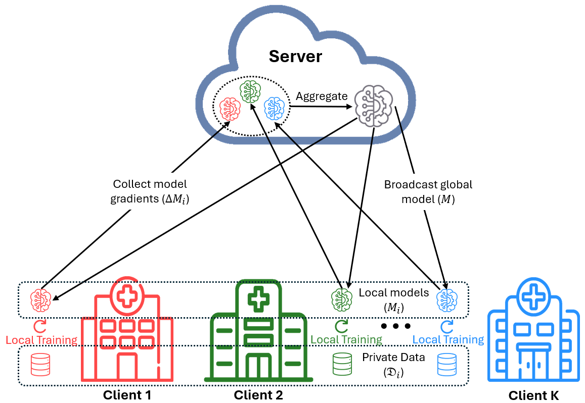
Figure 1: FL training process overview

Figure 1 presents an overview of the cross-silo FL training process, where participating clients train local models ($M_{i}$) on their datasets ($\mathcal{D}_{i}$), all based on a pre-distributed global model ($M$) [38, 48]. Instead of sharing raw data, clients exchange model updates ($M_{i}$) without sensitive information, aggregating centrally to enhance the global model. By utilizing a central server for coordination, silos transmit their updates, aggregated to improve the global model. This iterative process allows collaboration without compromising data privacy, as each client receives the updated global model without sharing raw data, ensuring data privacy while facilitating collaboration.

Data Skewness Types.

A centralized dataset $\mathcal{D}=\{(\mathbf{x}_{1},y_{1}),\dots,(\mathbf{x}_{n},y_{n})\}$, is a collection of $n$ tuples where $\mathbf{x}_{i}=[(x_{i})_{1},\dots,(x_{i})_{m}]$ is the feature representation of the $i$th element (sample) in the dataset, and $y_{i}\in\{1,\dots,\ell\}$ is the (true) label of the $i$th element.

In the FL setting, the dataset $\mathcal{D}$ is distributed over $K$ clients. We let $\mathcal{D}_{i}$ be the set of elements of the $i$th client. That is:

$$\mathcal{D}=\cup_{i=1}^{K}\mathcal{D}_{i}\qquad\text{and for $i\neq j$:}\qquad\mathcal{D}_{i}\cap\mathcal{D}_{j}=\emptyset.$$

Defining the type of non-IIDness in FL is relevant since it can drastically influence the performance of the models. We follow the settings of previous work [28, 50]. For a supervised learning task on client $i$ (local node $i$), we assume that each data sample $(x,y)\in\mathcal{D}_{i}$, where $x$ is the input attributes or features, and $y$ is the label, following a local distribution $P_{i}(\mathbf{x},y)$. Let us define:

$P_{i}^{Y}(y)=\sum_{\begin{subarray}{c}(\mathbf{x},z)\in\mathcal{D}_{i}\\ z=y\end{subarray}}P_{i}(\mathbf{x},z)\hskip 8.53581pt$

$P_{i}^{X_{\ell}}(x)=\sum_{\begin{subarray}{c}(\mathbf{x},y)\in\mathcal{D}_{i}\\ x_{\ell}=x\end{subarray}}P_{i}(\mathbf{x},y)$

with $P_{i}^{Y}(y)$, the $i$th client labels’ distribution and $P_{i}^{X_{\ell}}(x)$ the distribution over the $\ell$th input feature of the $i$th client. Then, the classification for non-IID data (i.e., data skewness types) is as follows:

• Regarding the concept of identically distributed:

  1. Label skew: Means that the label distribution $P_{i}^{Y}(y)$ of different clients is different.

  2. Feature skew: Occurs when the distribution of the features $P_{i}^{X_{\ell}}(x)$ varies from client to client.

  3. Quantity skew: Refers to the significant difference in the number of examples of different client data $P_{i}(\mathbf{x},y)$.

• Regarding the concept of independent:

  1. Spatiotemporal skewness: Refers to the inner correlation of data in the time (or space) domain. In other words, the distribution $P_{i}(\mathbf{x},y)$ is not stationary but depends on the time or space.

Quantifying the degree of non-IIDness.

Regarding the selection of valuable scenarios to demonstrate the effects of non-IIDness in FL, the current literature often relies on ad-hoc partitions [26, 21, 15]. Therefore, in this work, we use a metric that systematically evaluates the level of non-IID data to select scenarios for measuring the effect of non-IIDness. We opted for the Hellinger Distance (HD), a metric widely used to gauge the separation between two probability distributions calculated as in Equation 1 [12].

Aggregation and client selection algorithms

In an FL process, the server aggregates the weights obtained from each client and communicate them back to each participant. In this section, we explain the five state-of-the-art aggregation and client-selection algorithms assessed in our experiments.

FedAvg: It is a fundamental algorithm in FL [30] designed to train ML models across a network of decentralized devices while preserving data privacy. In FedAvg, each client computes model updates and sends them to a central server using local data. The server averages these updates to calculate a global model update and then sends it back to the clients. The latter process iterates until it convergences (the model’s performance gets stable).

FedProx: It is a framework designed to address heterogeneity in FL [24], offering a generalized and reparametrized version of FedAvg. This approach incorporates a regularization term ($\mu$) to minimize the difference between local and global weights. Finally, the framework aggregates local model updates from all devices to obtain an updated global model. Using this proximal term, FedProx aims to improve convergence and performance in heterogeneous federated learning environments.

Random size-proportional selection (Rand): Rand is a baseline client selection strategy introduced to handle non-IID data that does not bias toward clients with higher local losses. Most current analysis frameworks consider a scheme that selects the training set of clients $S(t)$ by sampling $m$ clients randomly (with replacement) such that client $k$ gets selected with probability $p_{k}$, the fraction of data at that client [6].

Power-Of-Choice (POC): The POC algorithm performs well under non-IID distribution. It is inspired by the power of $d$ choices load balancing strategy, which queueing systems commonly use [6], [7]. The central server first samples a candidate set of $d$ clients, where $d$ is between $m$ (the number of clients to be selected) and $K$. These candidates are chosen based on their data fraction ($p_{k}$). The server then sends the current global model to these candidates, who compute and return their local losses. Finally, the server selects $m$ clients with the highest losses to participate in the next training round. This approach aims to balance the workload and prioritize clients with more informative updates, improving the efficiency of the FL process.

Model Contrastive Learning (MOON): MOON is a simple and effective FL framework designed to tackle non-IIDness. It uses the similarity between model representations to correct the local training of individual parties (i.e., conducting contrastive learning at the model level) [23]. The network proposed in MOON has three components: a base encoder, a projection head, and an output layer. The base encoder extracts representation vectors from inputs. Le et al. introduce an additional projection head to map the representation to a space with a fixed dimension. Last, the output layer produces predicted values for each class. For ease of presentation, with model weight $w$, they use $F_{w}(\cdot)$ to denote the whole network and $R_{w}(\cdot)$ to denote the network before the output layer (i.e., $R_{w}(X_{\ell})$ is the mapped representation vector of input $X_{\ell}$).

IV Experimentation Setup

Datasets

This work considers six widely employed datasets to train the CL and FL models. Four of them, i.e., CIFAR10 [19], FMNIST [46], Physionet 2020 [14], Covtype [4], serve to simulate label, feature, and quantity skew, while the remaining two datasets, i.e., 5G Network Traffic flows [8], Snapshot Serengeti [41] work for spatiotemporal skew simulation. Table I summarizes the main characteristics of the datasets.

Table I: Characteristics of the datasets

Dataset	Type	#training examples	#test examples	#features	# classes	Class distr.
CIFAR10	Images	50,000	10,000	3,072	10	Balanced
FMNIST	Images	60,000	10,000	784	10	Balanced
Physionet	Tabular	39,895	2,095	120	27	Balanced
Covtype	Tabular	522,910	58,102	54	7	Unbalanced
Serengeti	Tabular	257,927	28,659	64	13	Unbalanced
5G NTF	Tabular	74,838	13,207	7	12	Unbalanced

Models

We adopt a well-studied convolutional neural network (CNN) broadly applied in computer vision [5] for the image datasets. It includes one input layer and three convolutional blocks—where the first two blocks each have a convolutional layer followed by a max pooling layer, and the final block contains a convolutional layer and a flattened layer. The initial convolutional layer has 32 filters, whereas the subsequent two layers each have 64 filters, all with a $3\times 3$ filter size and ReLu as the activation function. In the dense section of the network, there is one dense layer with 64 neurons using ReLu as the activation function. Additionally, we employ in our tests the transfer learning models EfficientNetB0 [42] and MobileNetV2 [39] since they produce higher classification power results for the datasets studied.

For the tabular datasets, we use a deep neural network (DNN), selected because it is widely employed in classification tasks with tabular data [37]. It comprises one input layer, three hidden layers, and one output layer [32]. The input layer uses as many units as the number of features used in the training set. The three layers contain 500 hidden units each, and the last layer is formed by considering the neurons equal to the number of classes to predict. Additionally, the hidden layers used the ReLu activation function and the output layer a SoftMax function. We use Adam as our optimizer with a learning rate of 0.001 for $K=30$ clients and a batch size of 64. We train the models for 40 communication rounds and ten local epochs for all aggregation algorithms except MOON, which is trained for 100 communication rounds. We run the experiments on all six datasets using five or ten different data partitions (i.e., five or ten random seeds).

IV-1 Hyperparameters tuning

For a fair comparison, we base our hyperparameter grids on the best-performing hyperparameters presented in the original papers as follows:

• Rand: The fraction of clients considered in each communication round gets fine-tuned from $\{0.3,0.5,0.7\}$ [6].

• FedProx: The $\mu$ parameter gets fine-tuned from {0, 0.001, 0.01, 0.1, 1, 10, 100} [24].

• POC: The parameter $C$ is equal to 0.5. The parameter $d$ gets fine-tuned from $\{15,18,19,21\}$ [6].

• MOON: The $\mu$ is tuned from the grid of $\{0.1,1,5,10\}$, and we find the best $\mu$ of 0.1, and we set the value of $temperature$ to 0.5 [23].

IV-A Methods for Synthetic Partitioning

The datasets introduced previously are all centralized, and we must split them while controlling the level of non-IIDness to train FL models. For such a purpose, we use the FedArtML [17] tool to partition each dataset among the clients. The following lines explain the partition method employed to simulate each skewness type.

IV-A1 Label Skew

We use the Dirichlet distribution (DD) to partition data among clients based on label distribution. The DD generates random numbers summing to one, controlled by parameter $\alpha$. Higher $\alpha$ values (e.g., 1000) create similar local distributions, while lower values increase the chance of clients having examples from a single, randomly chosen class [26]. Notice that the DD is the multivariate generalization of the Beta distribution, and the latter is the generalization of the Uniform distribution. Therefore, the partition of the datasets using DD is a skewed split of the data distribution [25].

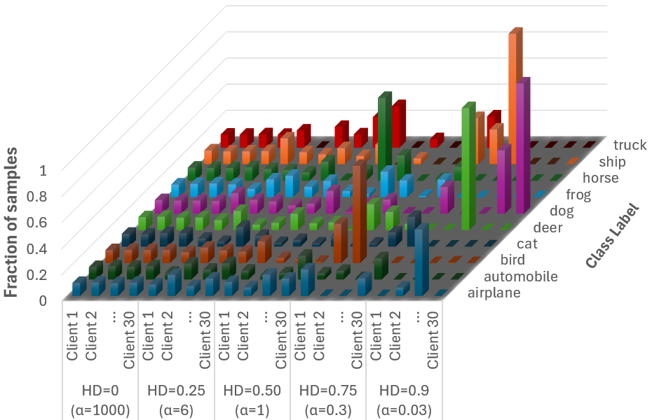
Figure 2: Distribution of CIFAR10 among 30 clients for different levels of non-IIDness.

We quantify the level of non-IIDness of the data partitions on the clients using the HD. Our levels of non-IIDness, quantified using HD, would be approximately equal to the following values: $\{0.0,0.25,0.5,0.75,0.9\}$. Fig. 2 exemplifies the partition distribution for label skew using thirty clients. All ten classes get evenly distributed among every client in the IID scenario ($\alpha=1000,\textsf{HD}=0.0$). As we increase the $\alpha$ parameter in the DD, the distribution of classes among clients becomes more diverse. In the extreme case of $\alpha=0.03,\textsf{HD}=0.9$, certain classes are absent in some local nodes.

IV-A2 Feature Skew

For simulating feature skew, we employed two diverse methods from FedArtML to test their properties:

Gaussian noise method: This approach introduces diverse Gaussian noise levels to each client’s local dataset to achieve diverse feature distributions. Specifically, for each client $i$, noise levels $\hat{x}$ are added according to the user-defined noise level $\sigma$, with $\hat{x}\sim\text{Gau}\left(\sigma\cdot\frac{i}{K}\right)$, where $\hat{x}$ represents the resultant features after applying the noise level to the original features. Here, $\text{Gau}\left(\sigma\cdot\frac{i}{K}\right)$ denotes a Gaussian distribution with a mean of 0 and a variance of $\sigma\cdot\frac{i}{K}$, and $K$ represents the total number of clients.

Hist-Dirichlet-based method: The process starts by characterizing the attributes of each client using other average values and then subjecting them to a binning procedure. Subsequently, it establishes the participation of each feature category within each client using the DD with a specified $\alpha$. Unlike the Gaussian Noise approach, this method distributes the data among the clients without modifying the features.

We measure the non-IIDness with the HD among the features across clients (FHD) within the range $\{0,0.25,0.5,0.75,0.9\}$.

IV-A3 Quantity Skew

We employ the MinSize-Dirichlet method, which specifies the DD’s $\alpha$ value and generates the desired participation proportions for each client. Subsequently, a minimum required size, which we refer to as “the minimum number of examples,” is established for each client. Thus, the minimum proportion size, denoted as $MinSize$, is calculated as $\textit{MinSize}=\frac{\textit{MinRequiredSize}}{n}$, where $n$ represents the total number of examples in the centralized dataset. If the designated proportions fall below MinSize, it substitutes them with MinSize. Finally, the proportions are normalized to fall from 0 to 1.

We assess the level of non-IIDness using the HD for quantity skew (QHD) within the range $\{0,0.10,0.17\}$.

IV-A4 Spatiotemporal (SPT) skew

The primary constraint in this partition process is that the dataset must contain a categorical variable of space (i.e., places, cities, latitude, longitude, etc.) or time (i.e., time, months, years, etc.) to use as the partitioning variable. For instance, Fig. 3 depicts the distribution of labels along the date of the 5GNTF dataset. In this case, the space variable employed to create the federated data is the flow’s date expressed in year-month-day format (categorical).

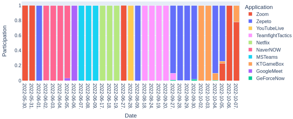
Figure 3: Distribution of 5GNTF applications (label) along date (spatiotemporal variable expressed in YYYY-MM-DD).

We use the St-Dirichlet method, which employs the DD to segment the data based on spatial (SP skew) or temporal (TMP skew) categories to distribute the data among federated clients. We assess the level of non-IIDness using the HD for spatiotemporal skew (STHD) within the range {0, 0.25, 0.5, 0.75, 0.9}.

IV-A5 Hardware Specification

We used an Ubuntu 22.04.4 LTS machine with 200 GB of disk, Intel(R) Xeon(R) Platinum 8259CL CPU @ 2.50GHz processor, 16 processors, 125 GB of RAM, and Python 3.10.12 to run the experiments. The FL models were trained using the Flower [2].

V Results and Highlights

This section depicts the main highlights and results of the experiments defined in Section IV. Each result gets grouped by label, feature, quantity, and spatiotemporal.

V-A Label Skew

This subsection examines how label skewness in the client data affects the models’ performance. Consider that the Covtype is an unbalanced dataset regarding the labels, and CIFAR10, FMNIST, and Physionet are balanced datasets. The accuracy of the models on each centralized dataset is our baseline for comparing the accuracy of the models generated in FL.

V-A1 Classification power

In this subsection, we focus on the findings from the simulations to compare different aggregation algorithms and datasets regarding their classification power (a.k.a accuracy).

Table II: Mean and standard deviation Accuracy for each dataset for CL, FedAvg, Rand, FedProx, Power-Of-Choice, and MOON, considering different levels of non-IIDness as measured by HD for $K=30$. Each model has undergone ten different trials.

Category	Dataset	HD	CL	FedAvg	Rand	FedProx	POC	MOON
Label distribution skew	CIFAR10	0	70.50% $\pm$ 0.60%	66.12% $\pm$ 0.73%	66.16% $\pm$ 0.74%	66.35% $\pm$ 0.72%	66.26% $\pm$ 0.70%	64.45% $\pm$ 1.05%
		0.25		65.91% $\pm$ 0.49%	65.49% $\pm$ 0.52%	65.86% $\pm$ 0.60%	65.61% $\pm$ 0.67%	63.40% $\pm$ 0.74%
		0.5		63.41% $\pm$ 0.95%	62.93% $\pm$ 1.55%	63.56% $\pm$ 0.83%	62.86% $\pm$ 1.71%	60.95% $\pm$ 1.33%
		0.75		58.85% $\pm$ 1.06%	56.80% $\pm$ 2.24%	58.80% $\pm$ 1.04%	55.84% $\pm$ 1.48%	55.27% $\pm$ 0.51%
		0.9		43.22% $\pm$ 2.24%	40.95% $\pm$ 2.43%	44.33% $\pm$ 2.83%	39.04% $\pm$ 2.99%	38.84% $\pm$ 2.31%
	FMNIST	0	90.90% $\pm$ 0.20%	90.68% $\pm$ 0.18%	90.63% $\pm$ 0.18%	90.69% $\pm$ 0.15%	90.62% $\pm$ 0.17%	88.70% $\pm$ 0.27%
		0.25		90.44% $\pm$ 0.14%	90.52% $\pm$ 0.17%	90.51% $\pm$ 0.17%	90.51% $\pm$ 0.18%	88.17% $\pm$ 0.22%
		0.5		89.92% $\pm$ 0.11%	89.84% $\pm$ 0.31%	89.96% $\pm$ 0.20%	89.74% $\pm$ 0.35%	87.37% $\pm$ 0.22%
		0.75		88.15% $\pm$ 0.54%	87.51% $\pm$ 0.81%	88.17% $\pm$ 0.47%	87.23% $\pm$ 0.78%	84.70% $\pm$ 0.84%
		0.9		80.37% $\pm$ 3.78%	79.08% $\pm$ 4.67%	81.10% $\pm$ 2.21%	77.83% $\pm$ 3.28%	70.79% $\pm$ 5.73%
	Physionet	0	63.74% $\pm$ 1.24%	57.97% $\pm$ 0.49%	57.48% $\pm$ 0.40%	58.16% $\pm$ 0.62%	57.86% $\pm$ 0.76%	61.80% $\pm$ 0.62%
		0.25		57.65% $\pm$ 0.47%	57.42% $\pm$ 0.54%	57.79% $\pm$ 0.55%	57.48% $\pm$ 0.53%	60.94% $\pm$ 0.60%
		0.5		55.69% $\pm$ 0.93%	55.26% $\pm$ 1.05%	56.29% $\pm$ 1.00%	55.24% $\pm$ 1.48%	58.76% $\pm$ 0.71%
		0.75		50.88% $\pm$ 1.18%	50.19% $\pm$ 2.07%	51.47% $\pm$ 1.20%	49.51% $\pm$ 2.30%	53.51% $\pm$ 1.37%
		0.9		41.35% $\pm$ 2.70%	39.68% $\pm$ 3.01%	41.95% $\pm$ 2.07%	38.81% $\pm$ 3.68%	42.49% $\pm$ 3.00%
	Covtype	0	95.60% $\pm$ 0.10%	94.95% $\pm$ 0.06%	94.89% $\pm$ 0.08%	94.96% $\pm$ 0.09%	94.84% $\pm$ 0.10%	95.64% $\pm$ 0.06%
		0.25		92.05% $\pm$ 1.14%	91.63% $\pm$ 1.52%	92.10% $\pm$ 1.28%	93.89% $\pm$ 0.73%	93.36% $\pm$ 1.18%
		0.5		84.92% $\pm$ 3.71%	83.10% $\pm$ 2.79%	85.54% $\pm$ 3.39%	88.21% $\pm$ 2.17%	84.61% $\pm$ 3.44%
		0.75		77.55% $\pm$ 3.63%	76.25% $\pm$ 4.10%	77.55% $\pm$ 3.64%	74.68% $\pm$ 5.31%	57.79% $\pm$ 12.66%
		0.9		59.10% $\pm$ 8.70%	59.02% $\pm$ 9.19%	59.46% $\pm$ 8.74%	57.29% $\pm$ 10.72%	50.51% $\pm$ 5.57%
Number of times that performed the best				3	1	8	2	6

Previous works claim that the data non-IIDness affects the performance of FL models [27, 29, 16]. Nevertheless, for the first time, we demonstrate that the effect of non-IIDness is not the same under all the levels of heterogeneity. Fig. 4 depicts the accuracy change by varying the level of non-IIDness of the data distributions among the clients measured by HD concerning the baseline model created in the centralized setting. As the non-IIDness of the data partitions increases, the model’s accuracy decreases. When the HD between data distributions of the clients exceeds 0.75, the drop becomes more drastic compared to previous levels.

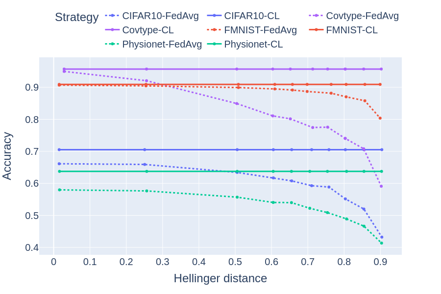
Figure 4: Changes in the models’ accuracy considering different levels of non-IIDness measured by HD for $K=30$.

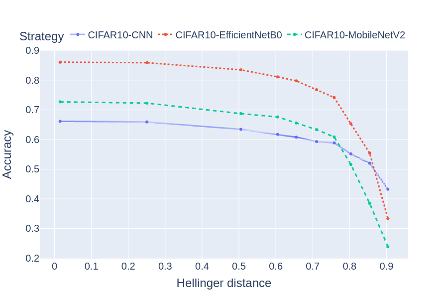
Figure 5: Changes in the models’ accuracy considering different levels of non-IIDness measured by HD for $K=30$ using CNN, EfficientNetB0 and MobilbeNetV2 on CIFAR10 dataset.

Fig. 5 illustrates the accuracy of models created using three different architectures: the CNN discussed earlier, EfficientNetB0, and MobileNetV2, both of which utilize transfer learning. The figure clearly shows a decline in model performance at the double thresholds after 0.5 and 0.75 HD. Notably, in pathological non-IID scenarios, the transfer learning models perform worse than our naive CNN model. This behavior can be attributed to the fact that only the last layers’ weights are updated locally, leading to skewed model weights and reducing the effectiveness of the aggregated model in capturing the overall dataset’s features, making transfer learning less suitable in such cases.

Consider the case when the HD is 0.9 (i.e., high non-IIDness) for all the datasets presented in Table II. When comparing the accuracy of Rand and POC versus their correspondent CL performance, those algorithms tend to have a higher drop in performance than the other aggregation methods. In FL scenarios with high non-IIDness, the distribution of data labels across clients is highly uneven. The latter means that specific clients may have more or different data types than others. Under such a scenario, Rand and POC may inadvertently select clients with skewed or unrepresentative data distributions, leading to poor generalization performance when aggregating their updates. MOON has the sharpest decrease in performance when the paradigm switches from CL to FL. Penalizing the current model with past and global representations made by each client will not help the model attain improved performance.

Table III: The performance’s decrease range of the model for the four datasets, moving from the lowest (HD=0) to the highest (HD=0.9) levels of non-IIDness and considering FedAvg.

Dataset	(HD=0) - (HD=0.9)
CIFAR10	22.9%
FMNIST	10.31%
Physionet	16.62%
Covtype	35.85%

Consider the IID case (i.e., HD = 0) and the most extreme non-IID case (i.e., HD = 0.9) for each dataset as depicted in Table III. Notice that the range of decrease in the reported performance (accuracy of HD=0 - accuracy of HD=0.9) is higher for the unbalanced dataset (Covtype) than for balanced datasets (CIFAR10, FMNIST, and Physionet). The more significant decrease in performance for unbalanced datasets can relate to the challenge of learning from skewed and less representative data. In non-IID scenarios, where clients have different class distributions, models trained on these unbalanced datasets may struggle to generalize well across clients.

V-A2 Convergence

In this subsection, we focus on the findings obtained using the CIFAR10 dataset to compare different aggregation algorithms regarding their learning process and the smoothness of training.

Table IV: The number of rounds required for FedAvg, Rand, FedProx, POC, and MOON to achieve 90% of the maximum accuracy reached in different levels of non-IID cases as determined by HD over CIFAR10 for K = 30.

Category	Dataset	Aggregation algorithm	HD = 0	HD = 0.25	HD = 0.5	HD = 0.75	HD = 0.9
Label distribution skew	CIFAR10	FedAvg	5	5	6	9	15
		Rand	5	5	6	10	14
		FedProx	5	5	6	9	15
		POC	5	5	6	8	15
		MOON	8	8	10	12	20

Table IV examines the algorithms’ convergence from a different perspective. We investigate the performance of each aggregation approach across a certain level of non-IID scenario independent from the others. For each specific non-IID situation described by HD, we determine how many rounds each aggregation algorithm requires to achieve 90% of its maximum accuracy. Therefore, regardless of the aggregation algorithm, as the non-IIDness of the data partitioning over the clients increases, more communication rounds are necessary to reach a convergence point (where the accuracy gets stable). We observe the latter because the data distributions among clients are sufficiently dissimilar, so the models built for each client are only optimal about their data, which diverges the model from the optimal case. As the training progresses, the weights delivered by the server to the clients improve because they get optimized by considering all of the data across all clients.

Table V: Mean and standard deviation Accuracy for each dataset for CL, FedAvg, Rand, FedProx, Power-Of-Choice, and MOON, considering different levels of feature skewness measured by FHD for K = 30. Each model has undergone ten different trials.

Category	Method	Dataset	FHD	CL	FedAvg	Rand	FedProx	POC	MOON
Feature distribution skew	Gaussian Noise	CIFAR10	0	70.50% $\pm$ 0.60%	66.12% $\pm$ 0.70%	66.16% $\pm$ 0.74%	66.35% $\pm$ 0.72%	66.26% $\pm$ 0.70%	64.45% $\pm$ 1.05%
			0.35	70.81% $\pm$ 0.45%	66.18% $\pm$ 0.57%	66.04% $\pm$ 0.44%	66.29% $\pm$ 0.63%	66.24% $\pm$ 0.50%	64.23% $\pm$ 0.53%
			0.75	70.44% $\pm$ 0.29%	66.17% $\pm$ 0.44%	66.31% $\pm$ 0.61%	66.36% $\pm$ 0.56%	66.27% $\pm$ 0.56%	64.58% $\pm$ 0.55%
			0.9	69.71% $\pm$ 0.03%	65.81% $\pm$ 0.82%	65.89% $\pm$ 0.72%	65.85% $\pm$ 0.68%	65.90% $\pm$ 0.77%	63.52% $\pm$ 0.66%
		FMNIST	0	90.90% $\pm$ 0.20%	90.68% $\pm$ 0.18%	90.57% $\pm$ 0.14%	90.69% $\pm$ 0.15%	90.62% $\pm$ 0.17%	88.70% $\pm$ 0.27%
			0.35	90.91% $\pm$ 0.26%	90.69% $\pm$ 0.19%	90.97% $\pm$ 0.15%	90.71% $\pm$ 0.17%	90.97% $\pm$ 0.17%	88.67% $\pm$ 0.28%
			0.75	90.96% $\pm$ 0.11%	90.54% $\pm$ 0.09%	90.53% $\pm$ 0.11%	90.57% $\pm$ 0.23%	90.51% $\pm$ 0.19%	88.64% $\pm$ 0.19%
			0.9	90.76% $\pm$ 0.13%	90.59% $\pm$ 0.09%	90.71% $\pm$ 0.15%	90.70% $\pm$ 0.29%	90.51% $\pm$ 0.11%	88.55% $\pm$ 0.21%
		Physionet	0	63.74% $\pm$ 1.24%	57.97% $\pm$ 0.49%	57.48% $\pm$ 0.40%	58.16% $\pm$ 0.62%	57.86% $\pm$ 0.76%	61.80% $\pm$ 0.62%
			0.35	63.30% $\pm$ 1.31%	57.89% $\pm$ 0.39%	57.92% $\pm$ 0.64%	58.08% $\pm$ 0.61%	57.47% $\pm$ 1.13%	61.22% $\pm$ 0.72%
			0.75	60.13% $\pm$ 1.11%	52.81% $\pm$ 0.83%	52.84% $\pm$ 0.74%	52.28% $\pm$ 0.38%	51.39% $\pm$ 0.25%	56.10% $\pm$ 0.90%
			0.9	28.97% $\pm$ 3.22%	29.43% $\pm$ 1.49%	29.88% $\pm$ 1.27%	29.43% $\pm$ 1.15%	25.25% $\pm$ 1.97%	32.06% $\pm$ 1.30%
		Covtype	0	95.60% $\pm$ 0.10%	94.95% $\pm$ 0.06%	94.89% $\pm$ 0.08%	94.96% $\pm$ 0.09%	94.84% $\pm$ 0.10%	95.53% $\pm$ 0.04%
			0.35	95.68% $\pm$ 0.10%	94.94% $\pm$ 0.06%	94.90% $\pm$ 0.04%	94.90% $\pm$ 0.08%	94.88% $\pm$ 0.08%	95.65% $\pm$ 0.06%
			0.75	95.53% $\pm$ 0.04%	94.79% $\pm$ 0.08%	94.62% $\pm$ 0.04%	94.74% $\pm$ 0.07%	94.68% $\pm$ 0.13%	95.11% $\pm$ 0.07%
			0.9	68.53% $\pm$ 1.49%	50.01% $\pm$ 0.35%	49.81% $\pm$ 0.50%	50.03% $\pm$ 0.42%	50.10% $\pm$ 1.67%	49.20% $\pm$ 0.11%
	Hist-Dirichlet	CIFAR10	0	70.50% $\pm$ 0.60%	66.42% $\pm$ 0.34%	66.35% $\pm$ 0.35%	66.21% $\pm$ 0.59%	66.40% $\pm$ 0.70%	64.79% $\pm$ 0.32%
			0.25		66.09% $\pm$ 0.49%	66.13% $\pm$ 0.48%	65.82% $\pm$ 0.46%	66.15% $\pm$ 0.53%	65.12% $\pm$ 0.85%
			0.5		66.30% $\pm$ 0.67%	66.04% $\pm$ 0.66%	66.22% $\pm$ 0.40%	66.52% $\pm$ 0.56%	64.52% $\pm$ 1.08%
			0.75		66.23% $\pm$ 0.33%	66.04% $\pm$ 0.67%	66.17% $\pm$ 0.55%	66.34% $\pm$ 0.51%	64.99% $\pm$ 0.31%
			0.9		66.25% $\pm$ 0.47%	65.25% $\pm$ 0.51%	65.25% $\pm$ 0.90%	66.17% $\pm$ 0.47%	64.12% $\pm$ 0.56%
		FMNIST	0	90.90% $\pm$ 0.20%	90.72% $\pm$ 0.20%	90.68% $\pm$ 0.12%	90.68% $\pm$ 0.15%	90.59% $\pm$ 0.22%	88.75% $\pm$ 0.13%
			0.25		90.62% $\pm$ 0.10%	90.66% $\pm$ 0.27%	90.70% $\pm$ 0.15%	90.62% $\pm$ 0.18%	88.72% $\pm$ 0.32%
			0.5		90.78% $\pm$ 0.12%	90.66% $\pm$ 0.09%	90.63% $\pm$ 0.17%	90.78% $\pm$ 0.23%	88.43% $\pm$ 0.30%
			0.75		90.53% $\pm$ 0.24%	90.67% $\pm$ 0.18%	90.73% $\pm$ 0.17%	90.56% $\pm$ 0.12%	88.26% $\pm$ 0.30%
			0.9		89.77% $\pm$ 0.32%	89.73% $\pm$ 0.35%	89.66% $\pm$ 0.24%	89.81% $\pm$ 0.29%	87.38% $\pm$ 0.16%
		Physionet	0	63.74% $\pm$ 1.24%	57.73% $\pm$ 0.72%	57.76% $\pm$ 0.51%	58.02% $\pm$ 0.76%	57.52% $\pm$ 0.68%	61.13% $\pm$ 0.42%
			0.25		57.67% $\pm$ 0.61%	57.62% $\pm$ 0.69%	58.16% $\pm$ 0.63%	57.05% $\pm$ 0.37%	61.91% $\pm$ 0.39%
			0.5		57.92% $\pm$ 0.40%	57.50% $\pm$ 0.68%	57.86% $\pm$ 0.33%	57.35% $\pm$ 0.47%	61.20% $\pm$ 0.83%
			0.75		57.27% $\pm$ 0.64%	57.18% $\pm$ 0.97%	57.34% $\pm$ 0.88%	56.99% $\pm$ 0.86%	62.11% $\pm$ 0.44%
			0.9		56.47% $\pm$ 0.80%	55.49% $\pm$ 1.34%	56.49% $\pm$ 0.60%	55.80% $\pm$ 1.24%	59.82% $\pm$ 1.02%
		Covtype	0	95.60% $\pm$ 0.10%	94.95% $\pm$ 0.03%	94.81% $\pm$ 0.02%	95.00% $\pm$ 0.03%	98.84% $\pm$ 0.09%	95.62% $\pm$ 0.11%
			0.25		94.95% $\pm$ 0.05%	94.83% $\pm$ 0.09%	94.97% $\pm$ 0.09%	94.77% $\pm$ 0.03%	95.63% $\pm$ 0.05%
			0.5		94.90% $\pm$ 0.02%	94.88% $\pm$ 0.11%	94.90% $\pm$ 0.07%	94.88% $\pm$ 0.02%	95.65% $\pm$ 0.02%
			0.75		94.80% $\pm$ 0.05%	94.67% $\pm$ 0.10%	94.78% $\pm$ 0.08%	94.74% $\pm$ 0.10%	95.57% $\pm$ 0.07%
			0.9		93.30% $\pm$ 0.42%	93.11% $\pm$ 0.52%	93.38% $\pm$ 0.31%	93.47% $\pm$ 0.33%	94.51% $\pm$ 0.07%
Number of times that performed the best					4	2	7	7	16

Furthermore, FedAvg, Rand, FedProx, and POC exhibit similar behavior in achieving a convergence point, and they do so after roughly the same number of communication rounds. On the other hand, MOON, as expected, requires more rounds to reach the same convergence state.

V-B Feature Skew

This section examines how feature skewness in the client data affects the models’ performance.

V-B1 Classification power

In this subsection, we focus on the findings from the simulations to compare different aggregation techniques and datasets regarding their classification power (a.k.a accuracy) in the presence of feature skew over the clients’ data. Table V summarizes the models’ performance derived from different aggregation algorithms under varying degrees of non-IID feature distributions, as indicated by FHD.

Transitioning the training methodology from CL to FL depicts a decline in the model’s performance, notably more pronounced in image datasets (CIFAR10) compared to tabular datasets (Covtype). This outcome is predictable since the model gets trained without access to the complete dataset, and each client optimizes the weights based on its available data. The more significant decrease observed in image datasets stems from the heightened complexity inherent in classification tasks compared to tabular datasets.

Consider only the image datasets (CIFAR10, FMNIST) and the models generated in FL. Regardless of the aggregation algorithm employed, the performance of the final model remains stable across different levels of feature non-IIDness, consistently converging to specific values for each aggregation method. The latter pattern could occur due to convolutional layers in image analysis, where alterations in specific pixel values have minimal impact on the outcome of the convolution process in the Gaussian-noise method.

Having tabular datasets (Covtype, Physionet) and using the Hist-Dirichlet approach shows that increasing the degree of feature non-IIDness does not impact the performance. However, when dealing with Gaussian noise, if we surpass FHD=0.9, there’s a noticeable decline in performance. This decline occurs because the data become so dissimilar (too noisy) from each other that even within the CL learning, the model struggles to learn from the data.

Table V validates that no particular algorithm outperforms others in image datasets, as they yield comparable final performance metrics. MOON emerges as the top-performing algorithm in both versions in tabular datasets, surpassing all other algorithms. Its performance is nearly equivalent to that of models trained in CL. The latter occurs since MOON can immediately start learning meaningful contrasts between differences in the label using the provided features of the tabular dataset. On the other hand, for images, the model first needs to learn to extract meaningful features from raw pixels before it can start contrasting different object classes effectively. For example, consider the Physionet dataset, which contains features such as age, sex, heart rate, and P-R interval. In that case, each feature has a clear medical interpretation, and the model can directly use the mentioned feature values without learning initial representations. Conversely, for CIFAR10, the model must learn to extract meaningful features from raw pixels before contrastive learning can be effective.

V-C Quantity Skew

This subsection examines how quantity skewness in the client data affects the models’ performance.

Table VI: Mean and standard deviation Accuracy for each dataset for CL, FedAvg, Rand, FedProx, Power-Of-Choice, and MOON, considering different levels of non-IID partitioning of the record quantities measured by QHD for $K=30$. Each model has undergone five different trials.

Category	Method	Dataset	CL	QHD	FedAvg	Rand	FedProx	POC	MOON
Quantity distribution skew	Min-size Dirichlet	CIFAR10	70.50% $\pm$ 0.6%	0	65.77% $\pm$ 0.57%	65.92% $\pm$ 0.72%	66.45% $\pm$ 0.61%	66.04% $\pm$ 0.35%	64.01% $\pm$ 0.46%
				0.10	66.69% $\pm$ 0.72%	66.29% $\pm$ 0.67%	66.71% $\pm$ 0.76%	68.82% $\pm$ 0.89%	63.24% $\pm$ 0.37%
				0.17	66.04% $\pm$ 0.65%	67.91% $\pm$ 0.46%	68.07% $\pm$ 0.42%	68.44% $\pm$ 0.51%	63.49% $\pm$ 1.25%
		FMNIST	90.90% $\pm$ 0.02%	0	90.72% $\pm$ 0.23%	90.69% $\pm$ 0.25%	90.64% $\pm$ 0.15%	90.67% $\pm$ 0.11%	88.49% $\pm$ 0.24%
				0.10	90.37% $\pm$ 0.16%	90.39% $\pm$ 0.22%	90.30% $\pm$ 0.45%	90.78% $\pm$ 0.13%	88.04% $\pm$ 0.27%
				0.17	90.39% $\pm$ 0.32%	90.43% $\pm$ 0.19%	90.44% $\pm$ 0.27%	90.65% $\pm$ 0.31%	88.10% $\pm$ 0.26%
		Physionet	63.74% $\pm$ 1.24%	0	58.23% $\pm$ 0.68%	57.13% $\pm$ 0.56%	58.04% $\pm$ 0.29%	57.08% $\pm$ 0.53%	61.29% $\pm$ 0.81%
				0.10	59.48% $\pm$ 2.09%	59.06% $\pm$ 1.71%	59.42% $\pm$ 1.23%	61.29% $\pm$ 0.50%	58.67% $\pm$ 1.97%
				0.17	64.22% $\pm$ 1.27%	64.40% $\pm$ 0.55%	64.92% $\pm$ 0.71%	64.82% $\pm$ 0.85%	63.86% $\pm$ 0.40%
		Covtype	95.60% $\pm$ 0.1%	0	94.97% $\pm$ 0.04%	94.87% $\pm$ 0.06%	94.96% $\pm$ 0.07%	94.83% $\pm$ 0.05%	95.15% $\pm$ 0.09%
				0.10	95.67% $\pm$ 0.10%	95.65% $\pm$ 0.07%	95.70% $\pm$ 0.10%	95.79% $\pm$ 0.10%	95.13% $\pm$ 0.12%
				0.17	90.65% $\pm$ 1.57%	94.77% $\pm$ 0.43%	95.27% $\pm$ 0.20%	94.94% $\pm$ 0.44%	94.23% $\pm$ 0.47%
Number of times that performed the best					1	0	3	6	2

V-C1 Convergence

In this subsection, we concentrate on the results of the simulations, aiming to contrast various aggregation methods and datasets in terms of their convergence.

Table VII: The number of rounds required for FedAvg, Rand, FedProx, POC, and MOON to achieve 90% of the maximum accuracy reached in different levels of feature non-IID cases as determined by FHD over CIFAR10 and Covtype using Hist Dirichlet for K = 30

Category	Method	Dataset	Aggregation algorithm	FHD = 0	FHD = 0.25	FHD = 0.50	FHD = 0.75	FHD = 0.9
Feature distribution skew	Hist Dirichlet	CIFAR10	FedAvg	5	5	5	5	4
			Rand	5	5	5	5	4
			FedProx	5	5	5	5	4
			POC	5	5	5	5	4
			MOON	8	7	7	8	7
		Covtype	FedAvg	3	3	3	3	4
			Rand	3	3	3	3	4
			FedProx	3	3	3	3	4
			POC	3	3	3	3	4
			MOON	4	4	4	4	5

Table VII presents an alternative viewpoint on the latter concept. It outlines the iterations needed for FedAvg, Rand, FedProx, POC, and MOON to achieve 90% of the maximum accuracy across various degrees of feature non-IID conditions, as characterized by FHD, using the CIFAR10 dataset. Increasing the non-IIDness of features within the data has minimal impact on the model’s ability to converge to its optimal performance.

V-C2 Classification power:

In the following paragraphs, we concentrate on the simulation results to evaluate various aggregation methods and datasets regarding their classification accuracy, particularly considering the impact of quantity skew on the clients’ data.

Examining Table VI and considering each aggregation algorithm separately, it is evident that the performance of the final models remains consistent across various levels of quantity skewness in the clients’ records. This phenomenon occurs regardless of the chosen aggregation algorithm, confirming that quantity skewness does not affect model performance.

V-C3 Convergence

In this subsection, we focus on the findings obtained when different aggregation algorithms regarding their learning process and the smoothness of training.

Table VIII: The number of rounds required for FedAvg, Rand, FedProx, POC, and MOON to achieve 90% of the maximum accuracy reached in different levels of quantity non-IID cases as determined by QHD over CIFAR10 and Covtype using Min-size Dirichlet method for K = 30

Category	Method	Dataset	Aggregation algorithm	QHD = 0	QHD = 0.10	QHD = 0.17
Quantity distribution skew	Min-size Dirichlet	CIFAR10	FedAvg	5	3	2
			Rand	5	3	1
			FedProx	5	3	2
			POC	5	3	2
			MOON	6	3	2
		Covtype	FedAvg	3	2	1
			Rand	3	2	1
			FedProx	3	2	1
			POC	3	2	1
			MOON	4	2	1

Looking at Table VIII, it is clear that regardless of the degree of non-IIDness in the number of records from each label across clients, all aggregation algorithms converge after a consistent number of communication rounds. This phenomenon occurs due to the similarity in data distributions among clients, where each client’s dataset mirrors others, making any information obtained from all clients also obtainable from just one client.

V-D Spatiotemporal Skew

This section examines how varying levels of data disparity among clients, based on time and location, impact model performance.

Table IX: Mean and standard deviation Accuracy for each dataset for CL, FedAvg, Rand, FedProx, Power-Of-Choice, and MOON, considering different levels of non-IID partitioning of the records based on their space (SP) and time (TMP) measured by STHD for $K=30$. Each model has undergone five trials.

Category	Type	Method	Dataset	CL	STHD	FedAvg	Rand	FedProx	POC	MOON
SPT distribution skew	SP skew	St-Dirichlet	Serengeti	96.95% $\pm$ 0.11%	0	95.58% $\pm$ 0.08%	95.56% $\pm$ 0.09%	95.62% $\pm$ 0.14	95.48% $\pm$ 0.09	96.69% $\pm$ 0.06
					0.25	95.63% $\pm$ 0.05%	95.50% $\pm$ 0.10%	95.64% $\pm$ 0.03	95.51% $\pm$ 0.11	96.76% $\pm$ 0.08
					0.5	95.40% $\pm$ 0.08%	95.32% $\pm$ 0.07%	95.36% $\pm$ 0.06	95.32% $\pm$ 0.06	96.51% $\pm$ 0.04
					0.75	94.09% $\pm$ 0.25%	93.91% $\pm$ 0.36%	94.15% $\pm$ 0.21	94.06% $\pm$ 0.09	95.80% $\pm$ 0.16
					0.9	88.65% $\pm$ 0.18%	87.68% $\pm$ 0.58%	88.49% $\pm$ 0.13	88.20% $\pm$ 0.39	91.74% $\pm$ 0.20
	TMP skew		5GNTF	92.39% $\pm$ 0.10%	0	92.15% $\pm$ 0.04%	92.15% $\pm$ 0.02%	92.14% $\pm$ 0.02%	92.15% $\pm$ 0.04%	92.23% $\pm$ 0.02%
					0.25	92.07% $\pm$ 0.12%	92.05% $\pm$ 0.15%	92.07% $\pm$ 0.18%	92.15% $\pm$ 0.05%	92.28% $\pm$ 0.04%
					0.5	88.28% $\pm$ 1.87%	87.92% $\pm$ 2.00%	89.19% $\pm$ 2.09%	92.08% $\pm$ 0.08%	89.24% $\pm$ 1.80%
					0.75	85.82% $\pm$ 0.06%	85.64% $\pm$ 0.08%	85.83% $\pm$ 0.08%	91.77% $\pm$ 0.32%	86.51% $\pm$ 1.79%
					0.9	84.62% $\pm$ 0.36%	84.50% $\pm$ 0.20%	84.55% $\pm$ 0.37%	89.23% $\pm$ 2.13%	83.94% $\pm$ 0.02%
Number of times that performed the best						0	0	0	3	7

Table X: Number of rounds required to achieve 90% of the maximum accuracy reached accuracy levels of spatiotemporal non-IID cases as determined by STHD for K = 30

Dataset	Aggregation algorithm	STHD = 0	STHD = 0.25	STHD = 0.50	STHD = 0.75	STHD = 0.9
Serengeti	FedAvg	6	7	7	10	14
	Rand	7	7	8	10	14
	FedProx	7	7	7	10	14
	POC	7	7	7	10	15
	MOON	8	8	9	12	19

V-D1 Classification power

In this subsection, we focus on the simulation results to evaluate various aggregation methods and datasets regarding classification accuracy. We pay particular attention to the impact of different levels of spatiotemporal skewness among the clients’ data.

Table IX demonstrates that irrespective of the aggregation algorithm employed, model performance deteriorates when data distribution among clients varies concerning time or space. This phenomenon occurs because increasing the differences among clients’ data based on time and location also raises the level of non-IIDness in the clients’ label distributions. This behavior is evident in Table XI, which displays the HD in label distributions at varying levels of STHD among clients. We also concluded in the Label Skew study section that higher levels of non-IIDness among clients’ data distributions negatively impact the performance of the final model.

V-D2 Convergence

In this subsection, we concentrate on our results related to the models’ convergence when there are variations in the data concerning time and location, considering the results obtained on Serengeti and 5GNTF datasets.

As shown in Table X, irrespective of the aggregation algorithm used for training, an increase in the distance between data distributions in terms of time and location results in a need for more rounds to achieve convergence. This trend is evident in both the Serengeti and 5GNTF datasets. When comparing the required rounds for STHD=0 and STHD=90, it is clear that in the worst case (STHD=90), the number of rounds needed is at least twice as high. This observation aligns with our earlier findings on classification performance, specifically from the Label Skew study, where we determined that higher non-IIDness among clients’ label distributions leads to increased rounds required to achieve convergence.

Table XI: HD among clients’ label distributions at varying levels of non-IID partitioning by time and space

Dataset	HD = 0	HD = 0.25	HD = 0.50	HD = 0.75	HD = 0.9
Serengeti	0.01	0.09	0.22	0.36	0.53
5GNTF	0.03	0.20	0.29	0.30	0.49

V-E General results

In this section, we provide highlights summarizing the overall results obtained from our experiments, combining the behavior shown before for label, feature, quantity, and spatiotemporal skewness.

Table XII: The number of cases in which each specific algorithm achieved the best performance for each study

Study	#Cases	FedAvg	Rand	FedProx	POC	MOON
Label Skew	20	3	1	8	2	6
Feature Skew	36	4	2	7	7	16
Quantity Skew	12	1	0	3	6	2
Spatio Temporal Skew	10	0	0	0	3	7
Total best performance		8	3	18	18	31

Table XII summarizes the cases in which each specific algorithm exhibited the best performance compared to other aggregation algorithms across four skewness types considered in our study. In most cases, the FedProx, POC, and MOON aggregation algorithms achieved the best performance, outperforming the simpler FedAvg and Rand algorithms.

Table XIII: The number of cases in which each aggregation algorithm achieved the best performance for each type of dataset

Dataset type	#Cases	FedAvg	Rand	FedProx	POC	MOON
Image	34	7	3	15	9	0
Tabular	44	1	0	3	9	31
Total best performance		8	3	18	18	31

Table XIII examines the best-performing aggregation algorithms from the perspective of the dataset type used for training. It shows that FedProx outperforms all other algorithms on image datasets in fifteen out of thirty-four cases. In comparison, MOON generally surpasses other algorithms on tabular datasets in thirty out of forty-four cases.

VI Design Insights and Opportunities

We provide some design insights and opportunities intending to help researchers direct their efforts toward solving the effects of data heterogeneity.

Quantifying non-IIDness.

Several works claim that the data non-IIDness affects the performance of FL models [27, 29, 16]. Nevertheless, for the first time, we demonstrate that the effect of the non-IIDness is not the same under all the levels of heterogeneity (see Fig. 4). Therefore, it is vital to quantify the non-IIDness level in FL. This work uses the HD metric to measure the data heterogeneity. However, we encourage researchers to test different metrics such as Jensen-Shannon distance [33], Earth mover’s distance [9], and Total Variation distance [3], among others.

Better methods to tackle high non-IIDness,

This work showcases how the state-of-the-art methods to tackle non-IIDness (Rand, POC, FedProx, MOON) perform against FedAvg. The conclusion is that no algorithm works better than FedAvg in all the scenarios. Moreover, the methods that work better do not show a vast improvement regarding FedAvg under high non-IID scenarios as their gain is at most two percent points. This phenomenon has also been studied and claimed in the scarce work of empirical analysis of non-IID data and methodologies [43, 1, 31, 22]. Therefore, creating methods to appropriately alleviate the effect of high data heterogeneity is needed to evolve and preserve FL. The latter aligns with the open problems reported by Kairouz et al. [18].

Focusing on highly unbalanced data,

In our experiments, we claim that the more significant decrease in performance comparing CL and FL occurs in unbalanced datasets since it relates to the challenge of learning from highly skewed and less representative data (see Table II). Thus, it is relevant to create solutions to tackle non-IIDness by considering the degree of unbalancedness that the labels might have across the clients.

Studying spatiotemporal skew.

To the time of writing of this work, no analyses or empirical studies about the effect of the spatiotemporal skew on the performance of FL models exist. Thus, for the first time, we produce experiments to understand how different levels of spatiotemporal non-IIDness affect the prediction power of an FL model. The results show (see Table IX) that high levels of space or time skewness decreases the performance of the models, more specifically when the HD is higher than 0.75 (severe non-IIDness). Thus, researchers may benchmark techniques to deal with space and time skew in FL [40, 11, 49] to determine the behavior under high data heterogeneity levels.

Methods to compare mixed non-IIDness types.

Current tools and methods for synthetic partitioning centralized data into federated data [17, 47, 20, 34, 15] focus on simulating one type of non-IIDness (label, feature, quantity, spatiotemporal skewness). Nevertheless, a more realistic scenario would be combining two or more types of data heterogeneity to evaluate how those mixes can alter the performance of FL models. Therefore, for research in FL purposes, it would be interesting to create methods to partition centralized data into federated clients that permit the control of non-IIDness level for each non-IIDness type at the same time.

VII Conclusions

This study provides a comprehensive empirical analysis of the non-IID effect in FL. We benchmarked five state-of-the-art strategies for handling non-IID data distributions under controlled conditions, exploring label, feature, quantity, and spatiotemporal skewness, with a novel focus on the latter. We aim to standardize the methodology for studying data heterogeneity in FL by using HD to quantify data distribution differences. Our findings reveal the significant impact of label and spatiotemporal skew non-IID types on FL model performance. We also demonstrate that the model’s performance drop appears at a double threshold. When HD is higher than 0.5 and 0.75, a higher damage and a steeper decrease in performance slope occurs. Moreover, our results suggest that the FL performance is heavily affected mainly when the non-IIDness is extreme. Thus, we offer valuable recommendations for researchers to address data heterogeneity. This work represents the most thorough examination of non-IIDness in FL to date, providing a robust foundation for future research in FL.

VIII Acknowledgments

Daniel Mauricio Jimenez G. and Andrea Vitaletti were partially supported by PNRR351 TECHNOPOLE – NEXT GEN EU Roma Technopole – Digital Transition, FP2 – Energy transition and digital transition in urban regeneration and construction and Sapienza Ateneo Research grant “La disintermediazione della Pubblica Amministrazione: il ruolo della tecnologia blockchain e le sue implicazioni nei processi e nei ruoli della PA.” Aris Anagnostopoulos was supported by the ERC Advanced Grant 788893 AMDROMA, the EC H2020RIA project “SoBigData++” (871042), the PNRR MUR project PE0000013-FAIR, the PNRR MUR project IR0000013-SoBigData.it, and the MUR PRIN project 2022EKNE5K “Learning in Markets and Society.” Ioannis Chatzigiannakis was supported by PE07-SERICS (Security and Rights in the Cyberspace) – European Union Next-Generation-EU-PE0000014 (Piano Nazionale di Ripresa e Resilienza – PNRR). Andrea Vitaletti was supported by PE11 - MICS (Made in Italy – Circular and Sustainable) – European Union Next-Generation-EU (Piano Nazionale di Ripresa e Resilienza – PNRR) and the project SERICS (PE00000014) under the MUR National Recovery and Resilience Plan funded by the European Union - NextGenerationEU.

Daniel Mauricio Jimenez Gutierrez is a Ph.D. student in Data Science with current research in Federated Machine Learning leveraged on data-driven problems at the Sapienza University of Rome. He holds an MSc. in Data Science magna cum laude (2022) and received a BSc. in Statistics at the National University of Colombia (2013). He was accepted to the Student’s Honours program at Sapienza for outstanding performance in the master’s course. He has applied ML and AI for almost ten years in credit risk and banking analytics. He was the Bureau Models’ Manager at Experian-Colombia.

Mehrdad Hassanzadeh is a master’s student in Data Science at Sapienza University. He holds a Bachelor’s degree in Computer Engineering with a concentration in Software. He has strong programming skills, particularly in Python, and has taught Python courses while serving as a teaching assistant in various subjects. His current research focuses on Federated Learning, and he has a deep interest in big data and distributed learning systems.

Aris Anagnostopoulos (http://aris.me) is a Professor in the Department of Computer, Control, and Management Engineering, Sapienza University of Rome, Italy. Before Sapienza, he was at Yahoo Research, Santa Clara, CA, USA. He received the Ph.D. degree in computer science from Brown University, Providence, RI, USA.

Ioannis Chatzigiannakis holds a Ph.D. from the University of Patras (2003) in the area of ad-hoc wireless mobile networks and a BEng from the University of Kent (1997) in Computer Systems Engineering. He is an Associate Professor at the Sapienza University of Rome in the Computer, Control, and Management Engineering Department. He has co-authored over 150 scientific publications in areas related to dynamic distributed computing, the Internet of Things, algorithm engineering, and software systems. He has been a project manager and site leader for numerous research & development projects funded by the EU in the context of H2020, FP7, FP6, and EDA. He has participated in the research & development teams of industrial projects. He actively participates in many open-source projects and regularly participates in open-source international events. He has started several technology-based start-ups related to the Internet of Things. He has served as the Secretary of the European Association for Theoretical Computer Science (EATCS).

Andrea Vitaletti holds a Ph.D. in Computer Engineering from SAPIENZA University of Rome (2002). He visited renowned international research centers such as ETHZ (CH) and AT&T Research Labs (USA). He is an Associate professor in networking and algorithmic topics at (DIAG) Dipartimento di Ingegneria informatica automatica e gestionale Antonio Ruberti University of Rome “La Sapienza.” He has (co-)authored more than 80 papers in journals and international conferences, mainly in algorithms and protocols for wireless and sensor networks and IoT. His current research interests concern the design and analysis of efficient IoT solutions and blockchain technologies. He has been involved in several EU projects as a researcher and PI and has founded 3 start-ups.

References

- [1] Ahmed M Abdelmoniem, Chen-Yu Ho, Pantelis Papageorgiou, and Marco Canini. Empirical analysis of federated learning in heterogeneous environments. In Proceedings of the 2nd European Workshop on Machine Learning and Systems, pages 1–9, 2022.
- [2] Daniel J Beutel, Taner Topal, Akhil Mathur, Xinchi Qiu, Javier Fernandez-Marques, Yan Gao, Lorenzo Sani, Kwing Hei Li, Titouan Parcollet, Pedro Porto Buarque de Gusmão, et al. Flower: A friendly federated learning research framework. arXiv preprint arXiv:2007.14390, 2020.
- [3] Arnab Bhattacharyya, Sutanu Gayen, Kuldeep S Meel, Dimitrios Myrisiotis, Aduri Pavan, and NV Vinodchandran. On approximating total variation distance. arXiv preprint arXiv:2206.07209, 2022.
- [4] Jock Blackard. Covertype. UCI Machine Learning Repository, 1998. DOI: https://doi.org/10.24432/C50K5N.
- [5] Rahul Chauhan, Kamal Kumar Ghanshala, and RC Joshi. Convolutional neural network (cnn) for image detection and recognition. In 2018 first international conference on secure cyber computing and communication (ICSCCC), pages 278–282, IEEE, 2018. IEEE, IEEE.
- [6] Yae Jee Cho, Jianyu Wang, and Gauri Joshi. Client selection in federated learning: Convergence analysis and power-of-choice selection strategies. arXiv preprint arXiv:2010.01243, 2020.
- [7] Yae Jee Cho, Jianyu Wang, and Gauri Joshi. Towards understanding biased client selection in federated learning. In International Conference on Artificial Intelligence and Statistics, pages 10351–10375. PMLR, 2022.
- [8] Yong-Hoon Choi, Daegyeom Kim, Myeongjin Ko, Kyung-yul Cheon, Seungkeun Park, Yunbae Kim, and Hyungoo Yoon. Ml-based 5g traffic generation for practical simulations using open datasets. IEEE Communications Magazine, 61(9):130–136, 2023.
- [9] Adam Davis, Tony Menzo, Ahmed Youssef, and Jure Zupan. Earth mover’s distance as a measure of cp violation. Journal of High Energy Physics, 2023(6):1–42, 2023.
- [10] Haya Elayan, Moayad Aloqaily, and Mohsen Guizani. Deep federated learning for iot-based decentralized healthcare systems. In 2021 International Wireless Communications and Mobile Computing (IWCMC), pages 105–109. IEEE, 2021.
- [11] Wenjie Fu, Xudong Zhang, Junlong Wang, Di Yang, Yuntong Lv, Yuqing Wang, Zhao Zhen, and Fei Wang. A spatiotemporal federated learning based distributed photovoltaic ultra-short-term power forecasting method. In 2023 IEEE/IAS 59th Industrial and Commercial Power Systems Technical Conference (I&CPS), pages 1–7. IEEE, 2023.
- [12] Roma Goussakov. Hellinger Distance-based Similarity Measures for Recommender Systems. PhD thesis, Umea University, 2020.
- [13] Mackenzie Graham, Richard Milne, Paige Fitzsimmons, and Mark Sheehan. Trust and the goldacre review: why trusted research environments are not about trust. Journal of Medical Ethics, 49(10):670–673, 2023.
- [14] Daniel Mauricio Jimenez Gutierrez, Hafiz Muuhammad Hassan, Lorella Landi, Andrea Vitaletti, and Ioannis Chatzigiannakis. Application of federated learning techniques for arrhythmia classification using 12-lead ecg signals. arXiv preprint arXiv:2208.10993, 2022.
- [15] Kevin Hsieh, Amar Phanishayee, Onur Mutlu, and Phillip Gibbons. The non-iid data quagmire of decentralized machine learning. In International Conference on Machine Learning, pages 4387–4398, unknown, 2020. PMLR, PMLR.
- [16] Hadi Jamali-Rad, Mohammad Abdizadeh, and Anuj Singh. Federated learning with taskonomy for non-iid data. IEEE transactions on neural networks and learning systems, 2022.
- [17] G Daniel Mauricio Jimenez, Aris Anagnostopoulos, Ioannis Chatzigiannakis, and Andrea Vitaletti. Fedartml: A tool to facilitate the generation of non-iid datasets in a controlled way to support federated learning research. IEEE Access, 2024.
- [18] Peter Kairouz, H Brendan McMahan, Brendan Avent, Aurélien Bellet, Mehdi Bennis, Arjun Nitin Bhagoji, Kallista Bonawitz, Zachary Charles, Graham Cormode, Rachel Cummings, et al. Advances and open problems in federated learning. Foundations and trends® in machine learning, 14(1–2):1–210, 2021.
- [19] Alex Krizhevsky, Vinod Nair, and Geoffrey Hinton. Cifar-10 (canadian institute for advanced research). unknown, 0(0):0, 2009.
- [20] Fan Lai, Yinwei Dai, Sanjay Singapuram, Jiachen Liu, Xiangfeng Zhu, Harsha Madhyastha, and Mosharaf Chowdhury. Fedscale: Benchmarking model and system performance of federated learning at scale. In International conference on machine learning, pages 11814–11827. PMLR, 2022.
- [21] Qinbin Li, Yiqun Diao, Quan Chen, and Bingsheng He. Federated learning on non-iid data silos: An experimental study. In 2022 IEEE 38th International Conference on Data Engineering (ICDE), pages 965–978, IEEE, 2022. IEEE, IEEE.
- [22] Qinbin Li, Yiqun Diao, Quan Chen, and Bingsheng He. Federated learning on non-iid data silos: An experimental study. In 2022 IEEE 38th international conference on data engineering (ICDE), pages 965–978. IEEE, 2022.
- [23] Qinbin Li, Bingsheng He, and Dawn Song. Model-contrastive federated learning. In Proceedings of the IEEE/CVF conference on computer vision and pattern recognition, pages 10713–10722, 2021.
- [24] Tian Li, Anit Kumar Sahu, Manzil Zaheer, Maziar Sanjabi, Ameet Talwalkar, and Virginia Smith. Federated optimization in heterogeneous networks. Proceedings of Machine learning and systems, 2:429–450, 2020.
- [25] Jiayu Lin. On the dirichlet distribution. Department of Mathematics and Statistics, Queens University, 40, 2016.
- [26] Tao Lin, Lingjing Kong, Sebastian U Stich, and Martin Jaggi. Ensemble distillation for robust model fusion in federated learning. Advances in Neural Information Processing Systems, 33:2351–2363, 2020.
- [27] Zili Lu, Heng Pan, Yueyue Dai, Xueming Si, and Yan Zhang. Federated learning with non-iid data: A survey. IEEE Internet of Things Journal, 2024.
- [28] Xiaodong Ma, Jia Zhu, Zhihao Lin, Shanxuan Chen, and Yangjie Qin. A state-of-the-art survey on solving non-iid data in federated learning. Future Generation Computer Systems, 135:244–258, 2022.
- [29] Xiaodong Ma, Jia Zhu, Zhihao Lin, Shanxuan Chen, and Yangjie Qin. A state-of-the-art survey on solving non-iid data in federated learning. Future Generation Computer Systems, 135:244–258, 2022.
- [30] Brendan McMahan, Eider Moore, Daniel Ramage, Seth Hampson, and Blaise Aguera y Arcas. Communication-efficient learning of deep networks from decentralized data. In Artificial intelligence and statistics, pages 1273–1282. PMLR, 2017.
- [31] Alessio Mora, Davide Fantini, and Paolo Bellavista. Federated learning algorithms with heterogeneous data distributions: An empirical evaluation. In 2022 IEEE/ACM 7th Symposium on Edge Computing (SEC), pages 336–341. IEEE, 2022.
- [32] Fatma Murat, Ozal Yildirim, Muhammed Talo, Ulas Baran Baloglu, Yakup Demir, and U. Rajendra Acharya. Application of deep learning techniques for heartbeats detection using ecg signals-analysis and review. Computers in Biology and Medicine, 120:103726, 2020.
- [33] Frank Nielsen. On the jensen–shannon symmetrization of distances relying on abstract means. Entropy, 21(5):485, 2019.
- [34] Jean Ogier du Terrail, Samy-Safwan Ayed, Edwige Cyffers, Felix Grimberg, Chaoyang He, Regis Loeb, Paul Mangold, Tanguy Marchand, Othmane Marfoq, Erum Mushtaq, et al. Flamby: Datasets and benchmarks for cross-silo federated learning in realistic healthcare settings. Advances in Neural Information Processing Systems, 35:5315–5334, 2022.
- [35] Debidutta Pattnaik, Sougata Ray, and Raghu Raman. Applications of artificial intelligence and machine learning in the financial services industry: A bibliometric review. Heliyon, 2024.
- [36] Anichur Rahman, Tanoy Debnath, Dipanjali Kundu, Md Saikat Islam Khan, Airin Afroj Aishi, Sadia Sazzad, Mohammad Sayduzzaman, and Shahab S Band. Machine learning and deep learning-based approach in smart healthcare: Recent advances, applications, challenges and opportunities. AIMS Public Health, 11(1):58–109, 2024.
- [37] Maryam Saeed, Olev Märtens, Benoit Larras, Antoine Frappé, Deepu John, and Barry Cardiff. Ecg classification with event-driven sampling. IEEE Access, 2024.
- [38] Sadman Sakib, Mostafa M Fouda, Zubair Md Fadlullah, Khalid Abualsaud, Elias Yaacoub, and Mohsen Guizani. Asynchronous federated learning-based ecg analysis for arrhythmia detection. In 2021 IEEE International Mediterranean Conference on Communications and Networking (MeditCom), pages 277–282. IEEE, 2021.
- [39] Mark Sandler, Andrew Howard, Menglong Zhu, Andrey Zhmoginov, and Liang-Chieh Chen. Mobilenetv2: Inverted residuals and linear bottlenecks. In Proceedings of the IEEE conference on computer vision and pattern recognition, pages 4510–4520, 2018.
- [40] Xiuyu Shen, Jingxu Chen, Siying Zhu, and Ran Yan. A decentralized federated learning-based spatial–temporal model for freight traffic speed forecasting. Expert Systems with Applications, 238:122302, 2024.
- [41] Alexandra Swanson, Margaret Kosmala, Chris Lintott, Robert Simpson, Arfon Smith, and Craig Packer. Snapshot serengeti, high-frequency annotated camera trap images of 40 mammalian species in an african savanna. Scientific data, 2(1):1–14, 2015.
- [42] Mingxing Tan and Quoc Le. Efficientnet: Rethinking model scaling for convolutional neural networks. In International conference on machine learning, pages 6105–6114. PMLR, 2019.
- [43] Saeed Vahidian, Mahdi Morafah, Mubarak Shah, and Bill Lin. Rethinking data heterogeneity in federated learning: Introducing a new notion and standard benchmarks. IEEE Transactions on Artificial Intelligence, 2023.
- [44] Yanmeng Wang, Qingjiang Shi, and Tsung-Hui Chang. Why batch normalization damage federated learning on non-iid data? IEEE Transactions on Neural Networks and Learning Systems, 2023.
- [45] Kok-Seng Wong, Manh Nguyen-Duc, Khiem Le-Huy, Long Ho-Tuan, Cuong Do-Danh, and Danh Le-Phuoc. An empirical study of federated learning on iot-edge devices: Resource allocation and heterogeneity. arXiv preprint arXiv:2305.19831, 2023.
- [46] Han Xiao, Kashif Rasul, and Roland Vollgraf. Fashion-mnist: a novel image dataset for benchmarking machine learning algorithms. arXiv preprint arXiv:1708.07747, 2017.
- [47] Dun Zeng, Siqi Liang, Xiangjing Hu, Hui Wang, and Zenglin Xu. Fedlab: A flexible federated learning framework. Journal of Machine Learning Research, 24(100):1–7, 2023.
- [48] Mufeng Zhang, Yining Wang, and Tao Luo. Federated learning for arrhythmia detection of non-iid ecg. In 2020 IEEE 6th International Conference on Computer and Communications (ICCC), pages 1176–1180. IEEE, 2020.
- [49] Xuehan Zhou, Ruimin Ke, Zhiyong Cui, Qiang Liu, and Wenxing Qian. Stfl: Spatio-temporal federated learning for vehicle trajectory prediction. In 2022 IEEE 2nd International Conference on Digital Twins and Parallel Intelligence (DTPI), pages 1–6. IEEE, 2022.
- [50] Hangyu Zhu, Jinjin Xu, Shiqing Liu, and Yaochu Jin. Federated learning on non-iid data: A survey. Neurocomputing, 465:371–390, 2021.