Safe On-Orbit Dislodging of Deployable Structures via Robust Adaptive MPC

Abstract

This paper proposes a novel robust adaptive model predictive controller for on-orbit dislodging. We consider the scenario where a servicer, equipped with a robot arm, must dislodge a client, a time-varying system composed of an underpowered jammed solar panel with a hybrid hinge system on a space station. Our approach leverages online set-membership identification to reduce the uncertainty to provide robust safety guarantees during dislodging despite bounded disturbances while balancing exploration and exploitation effectively in the parameter space. The feasibility of the developed robust adaptive MPC method is also examined through dislodging simulations and hardware experiments in zero-gravity and gravity environments, respectively. In addition, the advantages of our method are shown through comparison experiments with several state-of-the-art control schemes for both accuracy of parameter estimation and control performance.

I Introduction

On-orbit failures have frequently occurred ever since the first artificial satellite was launched into space [1, 2, 3, 4] due to various unpredictable reasons, e.g., debris collision, temperature, electromagnetic, etc. These failures have caused countless economic and scientific losses, which have become an enormous challenge in the past decades. On-orbit servicing leveraging autonomous robotics systems is an increasingly popular research topic for rescuing on-orbit failure [5, 6, 7, 8]. Additional complexity arises from the parameter uncertainty of the client satellite, the unpredictable nature of component failures and the constraints posed by limited sensory feedback [9], actuation power [10], and real-time decision making [11].

Dislodging an underpowered jammed component is one of the most common on-orbit maintenance tasks [12, 13, 14]. It involves safely manipulating objects that may be stuck or restrained due to various factors, such as microgravity [15], cold welding [16], stiction [13], or mechanical failure [2]. Dislodging a jammed component often requires applying significant, sudden force, which could potentially damage a delicate component. Few studies have considered using on-orbit robotics systems to address the problem. Previous work in [17] presented an adaptive control algorithm using a multi-robot system in a dislodging task for a solar panel. However, the algorithm did not consider safety constraints, which can lead to damage of both the servicer and client spacecraft. The risk of damage is exacerbated during the transient period when the adaptive controller is learning the system parameters. Although the adaptive controller is guaranteed to eventually learn the correct parameter, during the learning process, the adaptive controller can exert excessive force to dislodge the jammed component, potentially causing damage.

Online parameter estimation can be leveraged to address the challenge of uncertainty during servicing missions to guarantee safety. Adaptive control for updating controller parameters using real-time measurement data has been extensively studied and gained popularity in recent decades [18, 19, 20]. Traditional adaptive control methods, such as Model Reference Adaptive Control (MRAC) [21], adjust controller parameters to ensure the system follows a desired reference model but have the drawback of being sensitive to unmodeled dynamics and typically cannot handle state and input constraints. Failure to enforce constraints on both the manipulator and manipulated object may lead to component damage during the servicing [22], which can cause significant costs and lost time due to the need to replace aerospace components via relaunch.

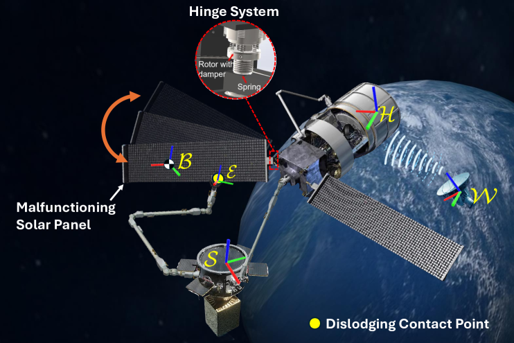
Figure 1: A servicer docked with a space station dislodges an underpowered solar panel with hinge via its robot arm in space. \hrefhttp://tiny.cc/tcst2025unm

Model predictive control (MPC) is a widely applied framework for managing uncertainties while ensuring constraint satisfaction and stability. In [23], an adaptive MPC algorithm for linear systems was introduced using a recursive approach, and its extension in [24] employed a tube-based framework to handle parametric uncertainty and additive disturbances in nonlinear systems. However, these methods rely on passive identification, preventing full exploitation of concurrent adaptation and control. A learning-based MPC in [25] used set-membership identification composed of two online phases: an adaptation phase with rigid tube-based robust MPC and a learning phase for uncertainty estimation, but only considers constant parameters, making it unsuitable for time-varying applications such as those found in aerospace. To address these limitations, this paper considers an adaptive controller that integrates set-membership identification to iteratively refine parameter bounds and employs robust MPC to ensure constraint enforcement and stability under worst-case conditions, ultimately improving performance as uncertainty estimates become less conservative.

In this paper, we propose a novel robust adaptive MPC with set-membership parameter estimation for the problem of safe dislodging. We demonstrate its implementation on our servicer during a dislodging task based on our client. The main contributions are summarized:

• Our robust adaptive MPC method provides robust guarantees on constraint enforcement despite the parametric uncertainty of the client and unpredictable failure modes.

• We transfer a specific hinge model with Euler-Lagrange form into a state-space equation and use our improved MPC algorithm for a dislodging task compared with two popular baselined methods to verify the feasibility and performance of our method in real applications.

• We develop a novel cost function that incorporates the time-varying parameter set with control input and state to improve the performance of parameter estimation during the control process.

Our robust adaptive MPC leverages dual-mode control [26] by incorporating time-varying parameter estimates into the MPC cost, balancing exploration which increases persistency of excitation to reduce uncertainty and exploitation which enhances control performance. Comparisons with a PID controller, adaptive control [17], and a state-of-the-art AMPC [25] demonstrate the superior performance and parameter estimation for time-varying systems. Moreover, our dual-state tube ensures safe parameter estimation within the initial set, remaining robust against future uncertainties.

Notation

The sets of real numbers and positive real numbers are denoted by $\mathbb{R}$ and $\mathbb{R}_{+}$, respectively. The sequence of integers from $n_{1}$ to $n_{2}$ is represented by $\{n_{1},n_{2}\}_{\mathbb{N}}=\{n\in\mathbb{N}\mid n_{1}\leq n\leq n_{2}\}$. For a vector $\mathbf{p}$, $\mathbf{p}{[i]}$ refers to its $i\text{-th}$ element. The $i\text{-th}$ row of a matrix $\mathbf{A}$ is denoted by $[\mathbf{A}]_{i}$. The Minkowski sum of two sets $\mathcal{A}$ and $\mathcal{B}$ is denoted by $\mathcal{A}\oplus\mathcal{B}$, and the pontryagin set difference of two sets can be denoted as $\mathcal{A}\ominus\mathcal{B}$. $\boldsymbol{\gamma}\in\mathbb{R}^{N}$ denotes a column vector with $N$ rows that each row contains a scalar value $\gamma$. The convex hull of the elements of a set S is represented by co{S}. We use $\mathbf{u}_{k}$ for the (real, measured) vector at time $k$ and $\mathbf{x}_{\varsigma|k}$ for the vector predicted $\varsigma$ steps ahead at time $k$. The estimated term is denoted with a ($\hat{\leavevmode\nobreak\ }$) on the top and the upper bound of a variable using ($\ \bar{}\$) on the top. The Center of Mass (CoM) is located at the position with distance from the pivot axis of the revolute joint as $d_{s}$. The dislodging contact position relative to the revolute joint is $d_{g}$. The angle between the gripper and the central axis of the rod is $\alpha$.

II On-Orbit Dislodging Problem

In this section, we define the dislodging problem for an underpowered jammed solar panel, preventing it from unfolding through its passive actuation system. Considering both unknown parameters and control input from the underpowered jammed solar panel and manipulator, respectively, with their constraints during dislodging, our objective is to keep safety not only for the control action but also for parameter estimation.

II-A Client and Servicer Agents

Let’s define the servicer and client agents and their interaction in the dislodging problem.

Client The client is a resident space object (RSO) with a malfunctioning solar panel. We assume the actuation system of the solar panel on its hinge is malfunctioning and cannot unfold the solar panel to the desired position. The solar panel is also jammed in a random position.

Servicer The servicer is a multi-functional spacecraft that can perform highly complicated repairing and servicing tasks. We assume that the servicer includes $1$ robotic arm with a gripper that can hold the solar panel to dislodge it into a specific position to unfold it.

We assume the frame $\mathcal{H}$ on the base of the client is stationary relative to frame $\mathcal{W}$ placed in the Earth as shown in Fig. 1. Considering the client can decouple the dynamics from the solar panel automatically by its inner stabilized system. This assumption holds during the whole process of dislodging.

Furthermore, we consider the client as a time-varying system in which the external environment may affect its stiffness properties, e.g., temperature, macro-gravity, vacuum conditions, radiation, etc., [27]. Also, we assume the dislodging contact location and orientation are ambiguous; the robot arm may not always be perpendicular to the rod, which means the $\alpha$ is not always $90^{\circ}$ and should also be time-varying as shown in Fig. 2. Hence, estimating unknown time-varying parameters for both the jammed component and grasping information during the dislodging under constraints becomes the biggest challenge in this task. We will pose this problem by dislodging the hinge from its initial position $\theta_{0}$ to a desired position $\theta^{*}$ with the calculated force applied by the servicer.

II-B Dislodging Dynamics

In this section, we model the dynamics of the client which is underpowered and to be dislodged by the servicer. The malfunctioning solar panel is modeled as an underpowered hybrid hinge [28] system whose dynamics can be modeled by the Euler-Lagrange equation in joint space as

$$\leavevmode\resizebox{427.47876pt}{}{$\mathbf{u}_{k}^{\top}\cdot\mathbf{r}_{\alpha}\times d_{g}=M{{\ddot{\theta}}_{k}}+C\dot{\theta}_{k}+\mathcal{\zeta}_{k}\dot{\theta}_{k}+\mathcal{K}_{k}\theta_{k}+\tau_{f}(\dot{\theta}_{k})+\tau_{m_{k}},$}$$ (1)

where $\theta_{k}$ is the angle of the hinge which has mass inertia $M\in\mathbb{R}_{+}$ and Coriolis and centripetal torque $C$. The spring-loaded hinge has stiffness $\mathcal{K}_{k}$ and viscous friction coefficient $\zeta_{k}$. The term

$$\tau_{f}(\dot{\theta})=-\mu\cdot r_{e}\cdot\tfrac{\dot{\theta}}{\left|\dot{\theta}\right|+\epsilon}$$

is the Coulomb friction of the hybrid hinge with material-dependent friction coefficient $\mu$; $r_{e}$ denote the effective radius of the rotor and $\epsilon\rightarrow 0\in\mathbb{R}_{+}$ to avoid the denominator to be zero. $\tau_{m_{k}}\in\{\tau_{m}\in\mathbb{R}:|\tau_{m}|\leq\delta_{\tau}\}$ denotes the external disturbance by the manipulator which is bounded through a constant value $\delta_{\tau}\in\mathbb{R}_{+}$ that affects the torque of the hinge.

The term $\mathbf{u}_{k}^{\top}\cdot\mathbf{r}_{\alpha}\times d_{g}$ describes the torque placed on the hinge by the servicer’s robotic arm where $\mathbf{r}_{\alpha}=\left[0,-\cos\alpha,\sin\alpha,0,0,0\right]^{\top}\in\mathbb{R}^{6}$ denotes the rotation vector for the end-effector (EE) of the robot arm on servicer relative to the perpendicular to the client; $\mathbf{u}_{k}{=}\begin{bmatrix}\mathbf{f}_{k},\boldsymbol{\tau}_{k}\end{bmatrix}^{\top}{\in}\ \mathbb{R}^{6}$ in which $\mathbf{f}_{k}{=}\left[{f_{x}}_{k},{f_{y}}_{k},{f_{z}}_{k}\right]^{\top}{\in}\mathbb{R}^{3}$ and $\boldsymbol{\tau}_{k}{=}\left[{\tau_{x}}_{k},{\tau_{y}}_{k},{\tau_{z}}_{k}\right]^{\top}{\in}\ \mathbb{R}^{3}$ denote the force and torque applied by the EE of the robot arm on the servicer to the dislodging contact point, respectively.

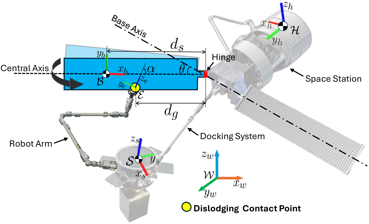
Figure 2: Diagram of the dislodging process that one servicer docks with a space station using its docking system and then dislodges a malfunctioning solar panel that is underpowered via its manipulator in space.

II-C Parametric Uncertainty

The dynamics (1) have parametric uncertainty. Specifically, the parameter vector $\boldsymbol{\rho}_{k}=[\mathcal{K}_{k},\zeta_{k},\mathcal{D}_{k}]^{\top}\in\mathbb{R}^{3}$ is an unknown and time-varying vector where $\mathcal{D}_{k}=d_{g}\cdot\sin(\alpha_{k})$ denotes the relative grasping positions of the gripper of the robot arm on the servicer; $\boldsymbol{\rho}^{*}_{k}$ is the true value of $\boldsymbol{\rho}_{k}$. We assume that at each time $k$ the parameter $\boldsymbol{\rho}_{k}$ belong to the known bounded polytope

$$\mathcal{P}:=\{\boldsymbol{\rho}_{k}\in\mathbb{R}^{3}|\mathbf{H}_{\rho}\boldsymbol{\rho}_{k}\leq\boldsymbol{\delta}_{\rho}\},$$ (2)

where $\boldsymbol{\rho}_{k}^{*}\in\mathcal{P}$ and $\mathbf{H}_{\rho}\in\mathbb{R}^{n_{p}\times 3}$. Furthermore, we assume the change in parameters is bounded. Specifically, we assume there exists a value $\varphi_{\rho}\in\mathbb{R}_{+}$ that satisfies $\boldsymbol{\rho}_{k}^{*}\in\mathcal{P}$ for $k\in\mathbb{N}$ that

$$\left\|\boldsymbol{\rho}_{k+1}^{*}-\boldsymbol{\rho}_{k}^{*}\right\|\leq\varphi_{\rho}.$$ (3)

II-D Safe Dislodging Constraints

To prevent damaging both the manipulator on the servicer and the jammed component during dislodging, we first need to enforce the input constraints

$$\mathcal{U}=\big{\{}\mathbf{u}\in\mathbb{R}^{6\times 1}\bigr{|}|\mathbf{u}_{k}^{\top}\cdot\mathbf{r}_{\alpha}\times d_{g}|\leq\bar{u}\big{\}},$$ (4a)

where $$\bar{u}\in\mathbb{R}_{+} k\in\mathbb{R}_{+} d_{g}$$ is the upper limits of the control input from the manipulator for all time . This constraint limits the force applied to the hinge to avoid damaging the jammed component. Enforcing this constraint is challenging since the contact point is unknown to the controller.

Likewise, to prevent damage, we need to enforce the state constraints

$$\mathcal{X}=\big{\{}\mathbf{x}\in\mathbb{R}^{2}\bigr{|}\mathbf{x}_{l}\leq\mathbf{x}_{k}\leq\mathbf{x}_{u}\big{\}}.$$ (4b)

where $\mathbf{x}_{l}=[\theta_{l},\dot{\theta}_{l}]^{\top}\in\mathbb{R}^{2\times 1}$ and $\mathbf{x}_{u}=[\theta_{u},\dot{\theta}_{u}]^{\top}\in\mathbb{R}^{2\times 1}$ denote the upper bound and lower bound of the state vector for all time $k\in\mathbb{R}_{+}$, respectively. The bounds $\mathbf{x}_{l}$ and $\mathbf{x}_{u}$ prevent overextending the hinge or causing the solar panel from colliding with another part of the client or servicer. Enforcing this constraint is challenging since it may require excessive force to stop the client before it overextends. Thus, by avoiding over-extension damage, we may cause excessive force damage.

II-E Safe On-Orbit Dislodging Problem

The safe on-orbit dislodging problem can be described as the servicer dislodges the client to regulate the client state $\mathbf{x}_{k}$ from the initial condition $\mathbf{x}_{0}$ to the desired equilibrium $\mathbf{x}^{*}$. Meanwhile, the parameter estimator can estimate the unknown time-varying parameter $\boldsymbol{\rho}_{k}$ to the true value $\boldsymbol{\rho}^{*}$ during the manipulation process. The objective can be described as

$$\left\{\begin{array}[]{l}\mathbf{e}_{x}=\displaystyle\lim_{k\rightarrow\infty}\lVert\mathbf{x}^{*}{-}\mathbf{x}_{k}\rVert_{2},\\ \mathbf{e}_{\rho}=\displaystyle\lim_{k\rightarrow\infty}\>\lVert\boldsymbol{\rho}^{*}{-}\boldsymbol{\rho}_{k}\rVert_{2}.\end{array}\right.$$ (5)

where $\mathbf{e}_{x}\in\mathbb{R}_{+}$ and $\mathbf{e}_{\rho}\in\mathbb{R}_{+}$ denote the state and parameter estimate error, respectively. While enforcing the safety constraint  (2), (8), (16), the hinge state should converge to the desired equilibrium and the uncertainty parameters should converge to their actual values. This requires balancing between the exploration to learn the uncertain parameters with bounded estimation errors and exploitation to use these bounds to ensure robust safety during dislodging.

III Robust Adaptive MPC for Dislodging

In this section, we introduce our robust adaptive MPC algorithm. This includes its set-membership parameter estimator, robust tube constraints, robust terminal set, and dual-mode cost function.

III-A Linear Parametric Modeling

To facilitate learning the uncertainty parameters $\boldsymbol{\rho}_{k}$, we reorganize the hinge dynamics (1) into the linear parametric state-space

$$\mathbf{x}_{k+1}=\left(\mathbf{I}+h\mathbf{A}(\boldsymbol{\rho}_{k})\right)\mathbf{x}_{k}+h\mathbf{B}(\boldsymbol{\rho}_{k})\mathbf{u}_{k}+\begin{bmatrix}0\\ {\dfrac{-\tau_{f}}{M}}\end{bmatrix}+\mathbf{w}_{k},$$ (6)

where $\mathbf{I}\in\mathbb{R}^{2\times 2}$ is the identity matrix, $\mathbf{x}_{k}=[\theta_{k},\dot{\theta}_{k}]^{\top}{\in}\mathbb{R}^{2}$ and $\mathbf{w}_{k}=\left[0,\tfrac{\tau_{s_{k}}}{M}\right]^{\top}{\in}\mathbb{R}^{2}$ denotes the disturbance which is bounded. $h\in(0,1)$ is the sampling period for discretization of the state matrices $\mathbf{A}(\boldsymbol{\rho}_{k})$ and $\mathbf{B}(\boldsymbol{\rho}_{k})$, in which can be parameterized as

$$\mathbf{A}(\boldsymbol{\rho}_{k}) =\mathbf{A}_{0}+\sum_{i=1}^{n}\mathbf{A}_{i}[\boldsymbol{\rho}_{k}]_{i},$$ (7)

$$\quad\mathbf{B}(\boldsymbol{\rho}_{k}) =\mathbf{B}_{0}+\sum_{i=1}^{n}\mathbf{B}_{i}[\boldsymbol{\rho}_{k}]_{i}.$$

Then based on (1), we can get (7) in detail as

$$\mathbf{A}(\boldsymbol{\rho}_{k}) =\begin{bmatrix}0&1\\ -\dfrac{\mathcal{K}_{k}}{M}&-\dfrac{\zeta_{k}}{M}\end{bmatrix}$$

$$\mathbf{B}(\boldsymbol{\rho}_{k}) =\frac{1}{M}\left[\begin{array}[]{cccccc}0&0&0&0&0&0\\ -\mathcal{D}_{k}&\mathcal{L}_{k}&0&0&0&1\end{array}\right]$$

Note that considering the gripper may not be perpendicular to the rod for all time during the dislodging task, $\alpha$ is also time-varying. Also, we assume the $\alpha$ would not deviate more than $70^{\circ}$ from the initial position and based on $\sin\theta=\sin(\pi+\phi)\approx-\phi$ and $\cos\theta=\cos(\pi+\phi)\approx-1$, we can use $-\phi$ and $-1$ to replace $\sin(\alpha_{k})$ and $\cos(\alpha_{k})$ respectively to get $\mathcal{D}_{k}=-d_{g}\cdot\phi_{k}$ and $\mathcal{L}_{k}=-1$.

III-B Set-Based Parameter Estimation

In this section, we present our set-based parameter estimator for dislodging in which bounds the uncertain parameters $\boldsymbol{\rho}_{k}$ of the linear parametric model (6) using real-time state $\mathbf{x}_{k}$ of the client and control input $\mathbf{u}_{k}$ from the servicer. Our robust adaptive MPC will leverage these bounds to ensure robust constraint satisfaction despite parametric uncertainty. To bound the parameter uncertainty, we make the following assumption about the boundedness of the measurement noise $\mathbf{w}_{k}$.

Assumption 1

The disturbance set $\mathbb{W}$ is a bounded polytope described by the $n_{w}$ constraints in the set

$$\mathbb{W}=\{\mathbf{w}_{k}\in\mathbb{R}^{2}|\mathbf{H}_{w}\mathbf{w}_{k}\leq\boldsymbol{\delta}_{w}\}.$$ (8)

where $\mathbf{H}_{w}\in\mathbb{R}^{n_{w}\times 2}$ and $\boldsymbol{\delta}_{w}\in\mathbb{R}^{n_{w}}$ The parameter set $\boldsymbol{\rho}_{k}$ are iteratively updated at each time step $k$ to form a set $\mathcal{P}_{k}$ which bounds all possible values of the uncertain parameters $\boldsymbol{\rho}_{k}$. This update is achieved by constructing a non-falsified parameter set, utilizing measurement data from the preceding $s$ time steps $\nu_{s}$, as follows:

$$\Delta_{k} :=\biggr{\{}\boldsymbol{\rho}_{k}\in\mathbb{R}^{p}\>\biggr{|}\mathbf{x}_{\nu_{s}+1}-\left(\mathbf{A}(\boldsymbol{\rho}_{k})\mathbf{x}_{\nu_{s}}+\mathbf{B}(\boldsymbol{\rho}_{k})\mathbf{u}_{\nu_{s}}\right)\in\mathbb{W}\biggr{\}}$$ (9)

$$=\biggr{\{}\boldsymbol{\rho}_{k}\in\mathbb{R}^{p}\>\biggr{|}\>-\mathbf{H}_{w}\mathbf{D}_{{\nu}_{s}{-}{1}}\boldsymbol{\rho}_{k}\leq\boldsymbol{\delta}_{w}+\mathbf{H}_{w}\mathbf{d}_{k}\biggr{\}},$$

where $\forall\nu_{s}{\in}\{k{-}s,k{-}1\}_{\mathbb{N}}$ denotes the preceding time steps from time $k{-}s$ to $k{-}1$, and $\mathbf{D}_{\nu_{s}}{\in}\mathbb{R}^{n\times 3}$ can be defined as

and $\mathbf{d}_{{\nu_{s}}+1}=\mathbf{A}_{0}\mathbf{x}_{\nu_{s}}+\mathbf{B}_{0}\mathbf{u}_{\nu_{s}}-\mathbf{x}_{{\nu_{s}}{+}{1}}$. Note that $\mathbf{D}_{\nu_{s}}$ and $\mathbf{d}_{\nu_{s}}$ are quantities that linearly depend on the measured state and input vectors, but the dependence is omitted for clarity. In this notion case, we can represent $\Delta$ using hyperplane constraints in $\mathbb{R}^{n}$, i.e., $\Delta$ is polytopic.

In (9), the non-falsified set $\Delta_{k}$ defines the set of all parameters that could have generated the measurement sequence $\{\mathbf{x}_{k-s},\ldots,\mathbf{x}_{k}\}$. To manage computational complexity, the polytopic set $\mathcal{P}_{k}$ is defined using a fixed number of linear constraints

$$\mathcal{P}_{k}:=\{\boldsymbol{\rho}_{k}\in\mathbb{R}^{3}|\mathbf{H}_{\rho_{k}}\boldsymbol{\rho}_{k}\leq\boldsymbol{\delta}_{\rho_{k}}\},$$ (11)

where the fixed matrix $\mathbf{H}_{\rho_{k}}\in\mathbb{R}^{n_{p}\times 3}$ is chosen offline and $\boldsymbol{\delta}_{\rho_{k}}\in\mathbb{R}^{n_{p}}$ is updated online. To account for the time-varying (3) parameters $\boldsymbol{\rho}_{k}^{*}$, we introduce a dilation operator with $\varsigma\in\mathbb{N}$ for $\mathcal{P}$ as

$$\mathbf{d}_{\varsigma}(\mathcal{P}):=\left\{\boldsymbol{\rho}_{k}\in\mathbb{R}^{p}\mid\mathbf{H}_{\rho_{k}}\boldsymbol{\rho}_{k}\leq\boldsymbol{\delta}_{\rho}+\varsigma\boldsymbol{\varphi}_{\rho}\boldsymbol{\gamma}\right\},$$ (12)

where the vector $\boldsymbol{\gamma}\in\mathbb{R}_{+}^{n_{\gamma}}$ and which dilates the constraints by a factor of $\varsigma\in\mathbb{N}$ in the direction $\boldsymbol{\varphi}_{\rho}$. Using the dilation operator (12), we have following the update rule for the uncertainty sets $\mathcal{P}_{k}$ bounding the parameter $\boldsymbol{\rho}_{k}$

$$\mathcal{P}_{k+1}:=\mathbf{d}_{\varsigma}\left(\mathcal{P}_{k}\cap\Delta_{k+1}\right)\cap\mathcal{P},$$ (13)

at time step $k$. Our robust adaptive MPC requires that we predict how the bounds $\hat{\mathcal{P}}_{\varsigma|k}$ on the time-varying parameters $\boldsymbol{\rho}_{k}$ evolve over the prediction horizon. These prediction bounds are given by

$$\hat{\mathcal{P}}_{\varsigma\mid k}=\mathbf{d}_{\varsigma}\left(\mathcal{P}_{{}_{k}}\right)\cap\mathcal{P},$$ (14)

for $\varsigma=1,\dots,N-1$ where $\hat{\mathcal{P}}_{\varsigma\mid k}$ is the predicted uncertainty bound at time $k+\varsigma$.

This is ensured by calculating $\boldsymbol{\delta}_{\rho_{k}}$ as a solution to the following set of linear programs:

$$\begin{split}[\boldsymbol{\delta}_{\rho_{k}}]_{i}\>&=\>\min_{\boldsymbol{\rho}\in\mathbb{R}^{p}}\quad[\boldsymbol{\delta}_{\rho}]_{i}\boldsymbol{\gamma}_{i},\quad\forall i\in\{1,n_{\rho^{+}}\}_{\mathbb{N}}\\ &\text{s. t. }\quad\begin{bmatrix}\mathbf{H}_{\rho}\\ -\mathbf{H}_{w}\mathbf{D}_{\nu_{s}}\end{bmatrix}\boldsymbol{\rho}^{+}\leq\begin{bmatrix}\boldsymbol{\delta}_{\rho_{k-1}}\\ \boldsymbol{\gamma}+\mathbf{H}_{w}\boldsymbol{d}_{k+1}\end{bmatrix}.\end{split}$$ (15)

III-C Robust Tube Constraints

In this section, we derive a state-space tube $\mathbb{X}_{\varsigma|k}$ for $\varsigma=1,\dots,N$ where $N$ is the prediction horizon and we can guarantee contains the state $\mathbf{x}_{k}$ despite parametric uncertainty $\boldsymbol{\rho}_{k}\in\mathcal{P}_{k}$ and disturbances $\mathbf{w}_{k}\in\mathbb{W}$. By remaining in the state tube, we can guarantee that the servicer would not damage the client. The states of the client and the control inputs from the servicer must satisfy the constraints as

$$\mathbb{Z} =\left\{(\mathbf{x}_{k},\mathbf{u}_{k})\in\mathbb{R}^{n}\times\mathbb{R}^{m}\bigr{|}\mathbf{F}\mathbf{x}_{k}+\mathbf{G}\mathbf{u}_{k}\leq\boldsymbol{\gamma}\right\},$$ (16)

where the matrices $\mathbf{F}\in\mathbb{R}^{n_{\gamma}\times n}$ and $\mathbf{G}\in\mathbb{R}^{n_{\gamma}\times n}$ are derived from the input (4a) and state (4b) constraints.

The tube MPC approach proposed in [29] ensures robust constraint satisfaction. The control input is parameterized using a feedback gain $\mathbf{K}\in\mathbb{R}^{m\times n}$ as

$$\mathbf{u}_{\varsigma|k}=\mathbf{K}\mathbf{x}_{\varsigma|k}+\mathbf{v}_{\varsigma|k},$$ (17)

where $\mathbf{v}_{N\mid k}=\left\{\mathbf{v}_{\varsigma\mid k}\right\}_{j\in\{0,N-1\}_{\mathbb{N}}}{\in}\mathbb{R}^{m}$ are decision variables in the MPC optimization problem. We make the following standard assumption about the feedback gain $\mathbf{K}$.

Assumption 2

The feedback gain $\mathbf{K}$ is chosen such that $\mathbf{A}_{\text{cl}}(\boldsymbol{\rho}_{k})=\mathbf{A}(\boldsymbol{\rho}_{k})+\mathbf{B}(\boldsymbol{\rho}_{k})\mathbf{K}$ is asymptotically stable $\forall\boldsymbol{\rho}_{k}\in\mathcal{P}\supseteq\mathcal{P}_{k}$.

A gain $\mathbf{K}$ satisfying Assumption 2 can be computed using standard robust control techniques, e.g., following the approach in [30].

The state tube is defined using the set-based dynamics

$$\mathbf{x}_{k} \in\mathbb{X}_{0|k},$$ (18a)

$$\mathbf{A}_{\text{cl}}(\boldsymbol{\rho}_{k})\mathbb{X}_{\varsigma|k}\oplus\mathbf{B}(\boldsymbol{\rho}_{k})\mathbf{u}_{\varsigma|k}\oplus\mathbb{W} \subseteq\mathbb{X}_{\varsigma+1|k},$$ (18b)

for $j=0,\dots,N-1$ and for all parameters $\boldsymbol{\rho}_{k}\in\mathcal{P}_{\varsigma|k}$. This ensures that $\mathbf{x}_{\varsigma|k}\in\mathbb{X}_{\varsigma|k}$ for all the realizations of uncertainty and disturbance. To manage computational complexity, the tube cross-section at each time step, $\left\{\mathbb{X}_{\varsigma\mid k}\right\}_{j\in\{0,N\}_{\mathbb{N}}}$, is parameterized by translating and scaling of the set

$$\mathbb{X}_{0}^{\curlyvee}:=\{\mathbf{x}\in\mathbb{R}^{n}|\mathbf{H}_{x}^{\curlyvee}\mathbf{x}\leq\boldsymbol{\gamma}\},$$ (19)

where the fixed matrix $\mathbf{H}_{x}$ is selected offline. Then, for $\varsigma=\{0,N\}_{\mathbb{N}}$, the state tube is parameterized as

where the $\{\mathbf{x}^{1},\mathbf{x}^{2},\ldots,\mathbf{x}^{v}\}$ are the vertices of the polytope (19). The variables $\mathbf{z}_{\varsigma|k}\in\mathbb{R}^{n}$ and $\vartheta_{\varsigma|k}\in\mathbb{R}_{+}$ are decision variables in the MPC optimization, which respectively define the translation and scaling of $\mathbb{X}_{0}$.

III-D Reformulation of Robust Tube Constraints

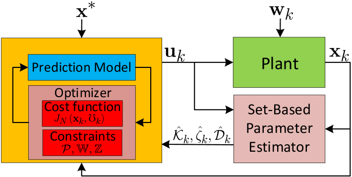
Figure 3: The block diagram of our robust adaptive MPC algorithm.

In this section, we present a convex formulation of the robust tube $\mathbb{X}_{\varsigma|k}$ which can be integrated into the MPC constraints to produce a tractable optimization problem. The state and input constraints defined in (16) and the set dynamics proposed in (18) must be robustly satisfied for all $\boldsymbol{\rho}\in\mathcal{P}_{k}$ and disturbances $\mathbf{w}\in\mathbb{W}$. To reformulate these in a convex manner, the following notation is defined

$$\mathbf{d}_{\varsigma|k}^{i} =\mathbf{A}_{0}\mathbf{x}_{\varsigma|k}^{i}+\mathbf{B}_{0}\mathbf{u}_{\varsigma|k}^{i}-\mathbf{z}_{\varsigma+1|k},$$ (21a)

$$\mathbf{D}_{\varsigma|k}^{i} =\mathbf{D}(\mathbf{x}_{\varsigma|k}^{i},\mathbf{u}_{\varsigma|k}^{i}),$$ (21b)

where $\mathbf{x}_{\varsigma|k}^{i}=\mathbf{z}_{\varsigma|k}+\vartheta_{\varsigma|k}\mathbf{x}^{i}$, $\mathbf{u}_{\varsigma|k}^{i}=\mathbf{K}\mathbf{x}_{\varsigma|k}^{i}+\boldsymbol{c}_{\varsigma|k}$, $i\in\{1,v\}_{\mathbb{N}},\varsigma\in\{0,N{-}1\}_{\mathbb{N}}$. Note that unlike the definition in (10) where $\mathbf{D}_{\nu_{s}},\mathbf{d}_{\nu_{s}}$ are a function of known states and inputs, the quantities $\mathbf{D}_{\varsigma|k}^{j},\mathbf{d}_{\varsigma|k}^{j}$ are linearly depend on the decision variables of MPC. Additionally, we define the vectors $\bar{\mathbf{f}}$ and $\bar{\mathbf{w}}$, which are computed offline such that for $i\in\{1,n_{c}\}_{\mathbb{N}},j\in\{1,n_{x}\}_{\mathbb{N}}$

_i $$=\max_{x\in\mathbb{X}_{0}}[\mathbf{F}+\mathbf{G}\mathbf{K}]_{i}\mathbf{x},$$ (22)

$$[\bar{\mathbf{w}}]_{j} =\max_{w\in\mathbb{W}}\>[\mathbf{H}_{x}]_{j}\mathbf{w}.$$

From [31], we can reformulate the robust tube constraints (20) as linear equality and inequality constraints as follows. Let the state tube $\{\mathbb{X}_{\varsigma|k}\}_{\varsigma\in\{{0},{N}\}_{\mathbb{N}}}$ be parameterized according to (20). Then, the constraints (16) and set-dynamics (18) are satisfied if and only if $\forall j\in\{1,v\}_{\mathbb{N}}$, $\varsigma\in\{0,N{-}1\}_{\mathbb{N}}$ there exists $\boldsymbol{\Gamma}_{\varsigma|k}^{j}\in\mathbb{R}^{n_{x}\times n_{p}}_{+}$ such that

$$(\mathbf{F}+\mathbf{G}\mathbf{K})\mathbf{z}_{\varsigma|k}+\mathbf{G}\mathbf{v}_{\varsigma|k}+\vartheta_{\varsigma|k}\bar{\boldsymbol{f}} \leq\boldsymbol{\gamma},$$ (23a)

$$-\mathbf{H}_{x}\mathbf{z}_{0|k}-\vartheta_{0|k}\boldsymbol{\gamma} \leq-\mathbf{H}_{x}\mathbf{x}_{k},$$ (23b)

$$\boldsymbol{\Gamma}_{\varsigma|k}^{j}\boldsymbol{\delta}_{\rho_{k}}+\mathbf{H}_{x}\mathbf{d}_{\varsigma|k}^{j}-\vartheta_{\varsigma+1|k}\boldsymbol{\gamma} \leq-\bar{\mathbf{w}},$$ (23c)

$$\mathbf{H}_{x}\mathbf{D}_{\varsigma|k}^{j} =\boldsymbol{\Gamma}_{\varsigma|k}^{j}\mathbf{H}_{\rho_{k}}.$$ (23d)

These linear inequality constraints allow the state tube constraints (20) to be incorporated as tractable constraints in the MPC optimization.

Similarly, we can also get the predicted state tube $\{\hat{\mathbb{X}}_{\varsigma|k}\}_{\varsigma\in\{{0},{\hat{N}-1}\}_{\mathbb{N}}}$ satisfy the set-dynamics (18) if and only if for all $j\in\{1,v\}_{\mathbb{N}}$ and $\varsigma\in\{0,\hat{N}{-}1\}_{\mathbb{N}}$ there exists $\hat{\boldsymbol{\Gamma}}_{\varsigma|k}^{i}\in\mathbb{R}^{n_{x}\times(n_{p}+n_{w})}_{+}$ such that

$$-\mathbf{H}_{x}\hat{\mathbf{z}}_{0|k}-\hat{\vartheta}_{0|k}\boldsymbol{\gamma} \leq-\mathbf{H}_{x}\mathbf{x}_{k},$$ (24a)

$$\hat{\mathbf{K}}_{\varsigma|k}^{i}\hat{\boldsymbol{\delta}}_{\rho_{k}}+\mathbf{H}_{x}\hat{\mathbf{d}}_{\varsigma|k}^{i}-\hat{\vartheta}_{\varsigma+1|k}\boldsymbol{\gamma} \leq-\bar{\mathbf{w}},$$ (24b)

$$\mathbf{H}_{x}\hat{\mathbf{D}}_{\varsigma|k}^{i} =\hat{\boldsymbol{\Gamma}}_{\varsigma|k}^{i}\hat{\mathbf{H}}_{\rho_{\varsigma|k}}.$$ (24c)

where $\hat{\mathbf{H}}_{\rho|k}=\left[\mathbf{\hat{H}}_{\rho_{k}}\ \mathbf{\hat{H}}_{\rho}\right]\in\mathbb{R}^{q_{k}^{\prime}\times p}$ and $\hat{\boldsymbol{\delta}}_{\rho_{k}}=\left[\boldsymbol{\delta}_{\rho_{k}}+\varsigma\boldsymbol{\gamma}\ \boldsymbol{\delta}_{\rho}\right]\in\mathbb{R}^{n_{p}}$. The constraints are bilinear in the variables since $\hat{\mathbf{H}}_{\rho},\hat{\boldsymbol{\delta}}_{\rho_{k}}$ are linearly dependent on the control input $\mathbf{u}_{k}$ as seen in (11).

III-E Robust Terminal Set

In this section, we derive a terminal set $\mathbb{X}_{\text{T}}$ which we will use to ensure our robust adaptive MPC is recursively feasible despite parametric uncertainty $\boldsymbol{\rho}_{k}\in\mathcal{P}$ and disturbances $\mathbf{w}_{k}\in\mathbb{W}$. Terminal constraints are imposed on $\mathbf{z}_{N|k}$ and $\vartheta_{N|k}$ so that the state tube constraints are directed into the terminal set to ensure the dislodging process in its final step does not lead the system into a region from which it could become unsafe in the future. We make the following assumption about the existence of a terminal set.

Assumption 3

There exists a nonempty terminal set $\mathbb{X}_{T}=\{(\mathbf{z},\vartheta)\in\mathbb{R}^{n}{\times}\mathbb{R}|\>\mathbf{z}{=}0,\>\vartheta{\in}[0,\bar{\vartheta}]\}$, such that for all $\boldsymbol{\rho}\in\mathcal{P}$ it holds that

$$(\mathbf{z},\vartheta)\in\mathbb{X}_{\text{T}}\Rightarrow \exists\left(\mathbf{z}^{+},\vartheta^{+}\right)\in\lambda\mathbb{X}_{\text{T}}\text{ s.t. }$$

$$\mathbf{A}_{\text{cl}}(\boldsymbol{\rho})\left(\{\mathbf{z}\}\oplus\vartheta\mathbb{X}_{0}\right)\subseteq\left\{\mathbf{z}^{+}\right\}\oplus\vartheta^{+}\mathbb{X}_{0}$$

$$(\mathbf{z},\vartheta)\in\mathbb{X}_{\text{T}}\Rightarrow \exists\left(\mathbf{z}^{+},\vartheta^{+}\right)\in\mathbb{X}_{\text{T}}\text{ s.t. }$$

$$\mathbf{A}_{\text{cl}}(\boldsymbol{\rho})\left(\{\mathbf{z}\}\oplus\vartheta\mathbb{X}_{0}\right)\oplus\mathbb{W}\subseteq\left\{\mathbf{z}^{+}\right\}\oplus\vartheta^{+}\mathbb{X}_{0}$$

$$(\mathbf{z},\vartheta)\in\mathbb{X}_{\text{T}}\Rightarrow (\mathbf{x},\mathbf{K}\mathbf{x})\in\mathbb{Z}\quad\forall\mathbf{x}\in\{\mathbf{z}\}\oplus\vartheta\mathbb{X}_{0}$$

Assumption 3 implies that the set $\mathbb{X}_{T}$ is a robust positively invariant (RPI) set for the set-dynamics in $(\mathbf{z},\vartheta)$, with an additional constraint that the set $\mathbb{X}_{N|k}$ remains centered at origin. Note that Assumption 2 is a necessary condition for Assumption 3 to be satisfied, but they are stated separately to emphasize that the stronger assumption is only needed to implement the terminal condition.

III-F Robust Adaptive MPC Algorithm

In this section, we present our robust adaptive MPC algorithm for the safe on-orbit dislodging problem.

First, we define our double-safe cost function formulated as

$$J_{N}(\mathbf{x}_{k},\boldsymbol{\mho}_{k})=\sum_{i=0}^{N-1}\ell\left(\mathbb{X}_{i\mid k},\mathbf{v}_{i\mid k}\right)+\ell\left(\mathbb{X}_{N\mid k}\right),$$ (25)

with $\boldsymbol{\mho}=\bigl{\{}\{\mathbf{z}_{\varsigma|k}\},\{\vartheta_{\varsigma|k}\},\{\mathbf{v}_{\varsigma|k}\},\{\mathbf{K}^{j}_{\varsigma|k}\}\bigl{\}}$ as the decision variable. $\ell\left(\mathbb{X}_{i\mid k},\mathbf{v}_{i\mid k}\right)=\max_{\mathbf{x}\in\mathbb{X}}||\mathbf{Q}\mathbf{x}||_{\infty}+||\mathbf{R}(\mathbf{K}\mathbf{x}+\mathbf{v})||_{\infty}+||\boldsymbol{\Upsilon}\boldsymbol{\rho}||_{\infty}$, and $\mathbf{Q},\mathbf{R},\boldsymbol{\Upsilon}$ are positive definite matrices. Note that in our work, we introduce the term $||\boldsymbol{\Upsilon}\boldsymbol{\rho}||_{\infty}$ which explicitly optimizing not only for the system’s control performance but also for improving the accuracy of your time-varying parameter estimates. The results for parameter estimation in Section IV evidently shows the advantage of this novel contribution compared with traditional adaptive MPC. A linear cost function is selected to enable its reformulation through linear inequalities resulting in the MPC optimization problem becoming a linear program.

Algorithm 1 Robust Adaptive MPC in parameter exploration

1:Input Choose $\mathbf{K}$, $\bar{\vartheta}$, and $\mathbb{X}_{0}$. Initialize $\boldsymbol{\delta}_{\rho_{k}}$ and $\hat{\boldsymbol{\rho}}_{k}$. Determine $\mathbf{Q},\mathbf{R},\boldsymbol{\Upsilon}$ for (25)

2:Online

3:$k\leftarrow 0$

4:for $k=0$ to $N$ do

5:  Obtain the measurement $\mathbf{x}_{k}$

6:  Construct $\Delta_{k}$ according to (9)

7:  Update $\mathcal{P}_{k}$ using (13)

8:  Update $\boldsymbol{\delta}_{\rho_{k}}$ using (15) and compute $\hat{\boldsymbol{\rho}}_{k}$

9:  Solve optimization problem (26)

10:  Apply the control input $\mathbf{u}_{k}=\mathbf{K}\mathbf{x}_{k}+\mathbf{v}_{0|k}$

11:  $k\leftarrow k+1$

12:end for

Then, the optimization problem can be written as

$$\begin{array}[]{r}\min J_{N}\left(\mathbf{x}_{k},\boldsymbol{\mho}_{k}\right)\\ \text{ s.t. }\eqref{eq:lambdaConstraints},\eqref{eq:lambda_tilConstraints}.\end{array}$$ (26)

The block diagram of the whole algorithm as shown in Fig. 3 and the following proposition show that our robust adaptive MPC enforces the dislodging constraints despite parametric uncertainty.

Parameter	$m$	$d_{s}$	$d_{g}$	$\mu$	$r_{e}$	$I_{cm}$	$J_{m}$	$\mathcal{K}_{k}$	$\zeta_{k}$	$\mathcal{D}_{k}$
Value	1.8 kg	1.2 m	2.5 m	0.3	0.2 m	1.5 kg/m2	4.1 kg/m2	$0.45+0.1\sin(0.1k)$	$0.6+0.15\sin(0.1k)$	$2.5+0.2\sin(0.1k)$

Table I: Simulation parameters for the time-varying system in the dislodging task.

Theorem 1: Let the assumptions 1, 2 and 3 be satisfied and an initial feasible solution exist. Let the parameter estimate set $\mathcal{P}_{k}$ be defined by the set dynamics (13) and admissible input set $\mathcal{I}_{v_{s}}\left(\mathbf{x}_{k},\mathcal{P}_{k}\right)$ as

Then, the closed loop system using Algorithm 1 satisfies the following properties for all $k>k_{0}$:

1. $\boldsymbol{\rho}_{k}\in\mathcal{P}_{k}$

2. $\mathcal{I}_{v_{s}}\neq\{\varnothing\}$

3. $(\mathbf{x}_{k},\mathbf{u}_{k})\in\mathbb{Z}$.

Proof:

For Property (1), we know that $\boldsymbol{\rho}_{k}\in\mathcal{P}_{k}$ and define $\epsilon_{\rho_{k}}=\boldsymbol{\rho}_{k+1}-\boldsymbol{\rho}_{k}$. Then we can get

$$\mathcal{P}_{k}\cap\Delta_{k+1}=\left\{\boldsymbol{\rho}_{k}\in\mathbb{R}^{3}\mid\tilde{\mathbf{H}}_{\theta_{k}}\boldsymbol{\rho}_{k}\leq\tilde{\boldsymbol{\delta}}_{\rho_{k}}\right\}.$$

After that, we can get

$$\tilde{\mathbf{H}}_{\rho_{k}}\boldsymbol{\rho}_{k+1}=\tilde{\mathbf{H}}_{\rho_{k}}\boldsymbol{\rho}_{k}+\tilde{\mathbf{H}}_{\rho_{k}}\epsilon_{\rho_{k}}\leq\tilde{\boldsymbol{\delta}}_{\rho_{k}}+d_{\rho}\boldsymbol{\gamma}.$$

Since by assumption $\boldsymbol{\rho}_{k+1}\in\mathcal{P}$, we can get $\boldsymbol{\rho}_{k+1}\in\mathbf{d}_{\varsigma}\left(\mathcal{P}_{k}\cap\Delta_{k+1}\right)$.

For Property(2), since we know that

$$\mathcal{P}_{\varsigma\mid k+1}=\mathbf{d}_{\varsigma+1}\left(\mathcal{P}_{k}\right)\cap\mathcal{P}=\mathcal{P}_{\varsigma+1|k}.$$

Then we have

$$\tilde{\mathbb{X}}_{\varsigma+1\mid k+1}\supseteq\mathbf{A}_{\text{cl}}(\boldsymbol{\rho})\tilde{\mathbb{X}}_{\varsigma\mid k+1}\oplus\mathbf{B}(\theta)\tilde{\mathbf{v}}_{\varsigma\mid k+1}\oplus\mathbb{W}.$$

where $\tilde{\mathbf{v}}_{\varsigma\mid k+1}=\mathbf{v}_{\varsigma+1\mid k}^{*}$ and $\varsigma\in\{0,N{-}2\}_{\mathbb{N}}$. Based on Assumption 3 that there exist $\mathbb{X}_{N\mid k+1}$ satisfy the last set when $\varsigma=N{-}1$, that proof that $\mathcal{I}_{v_{s}}\neq\{\varnothing\}$ during all time step.

Property (3) is the direct result of Section III-D.

∎

IV Simulation results

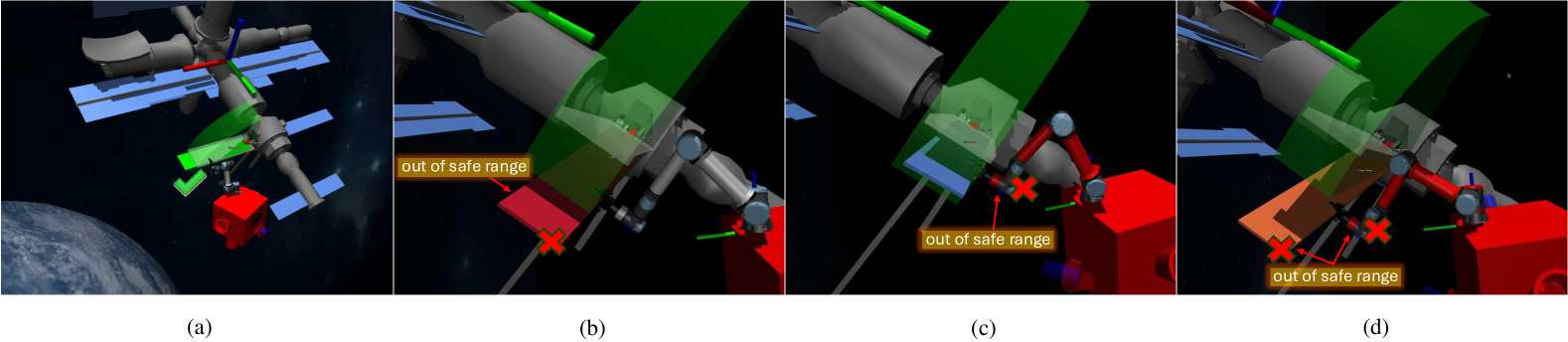
Figure 4: Dislodging mission using a servicer which contains simulated on MuJoCo Platform in a zero-gravity environment.

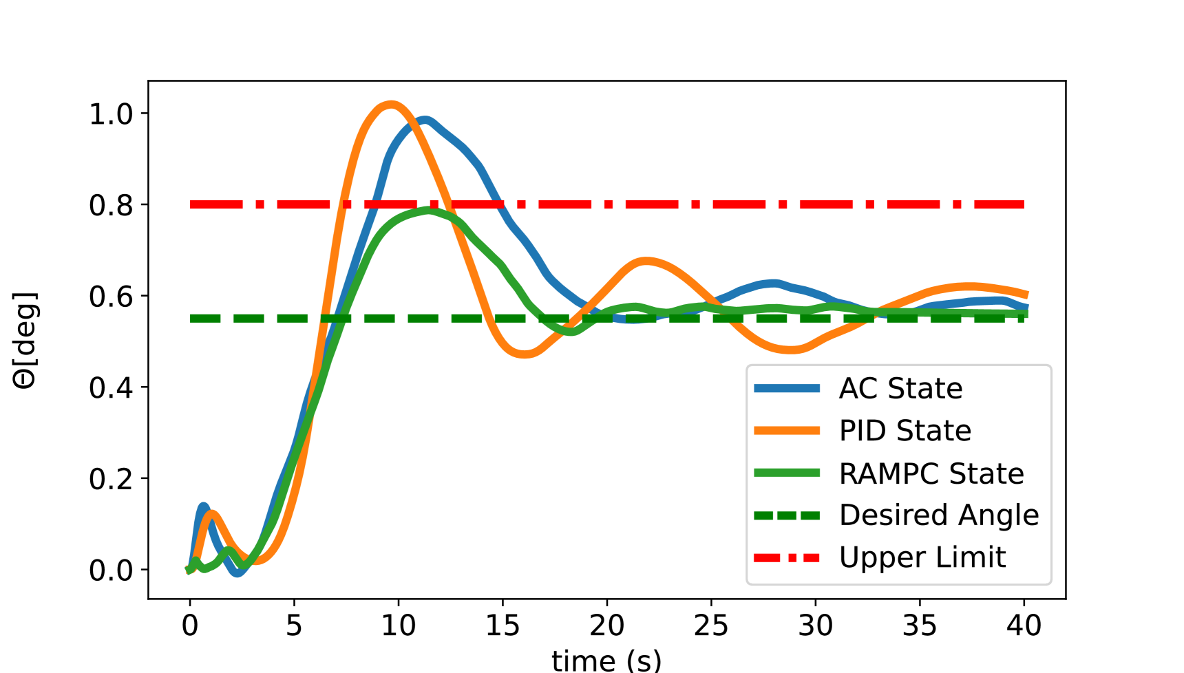
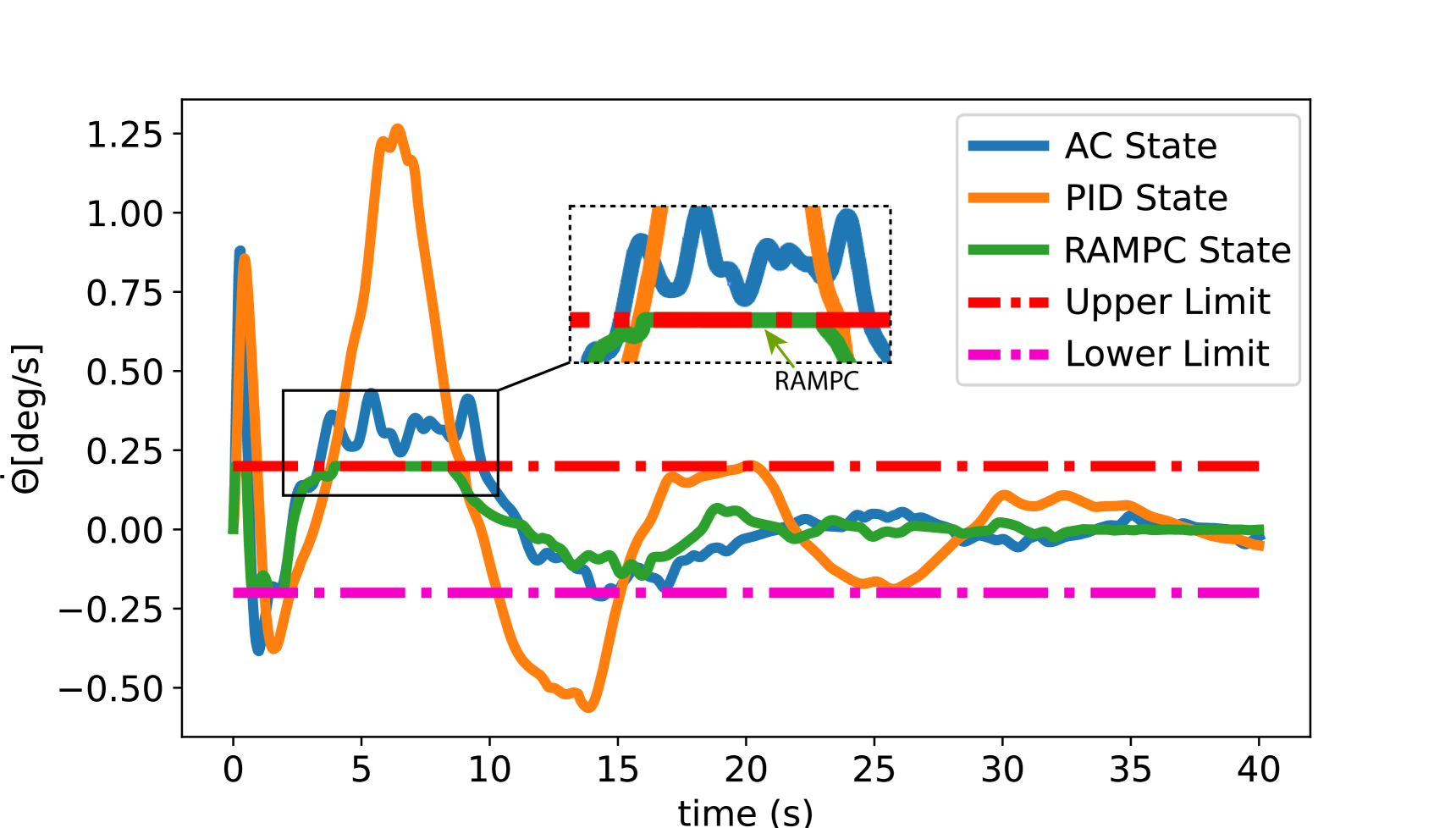
((a))

((b))

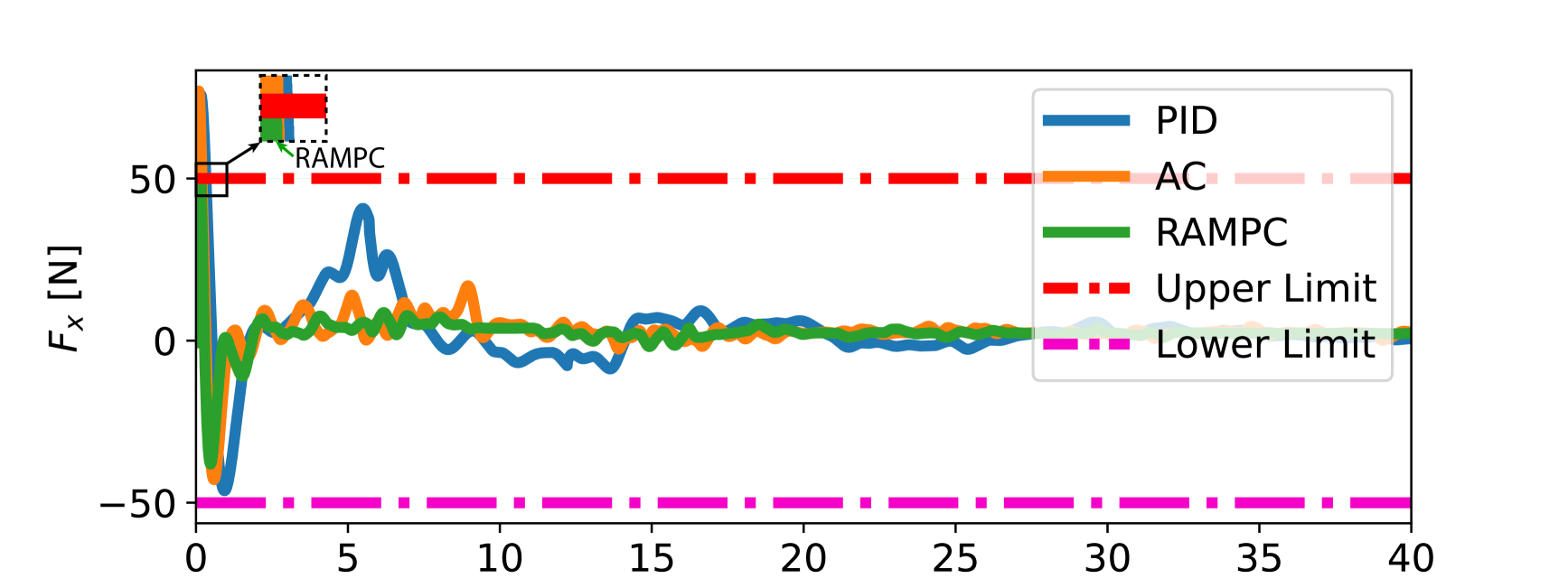
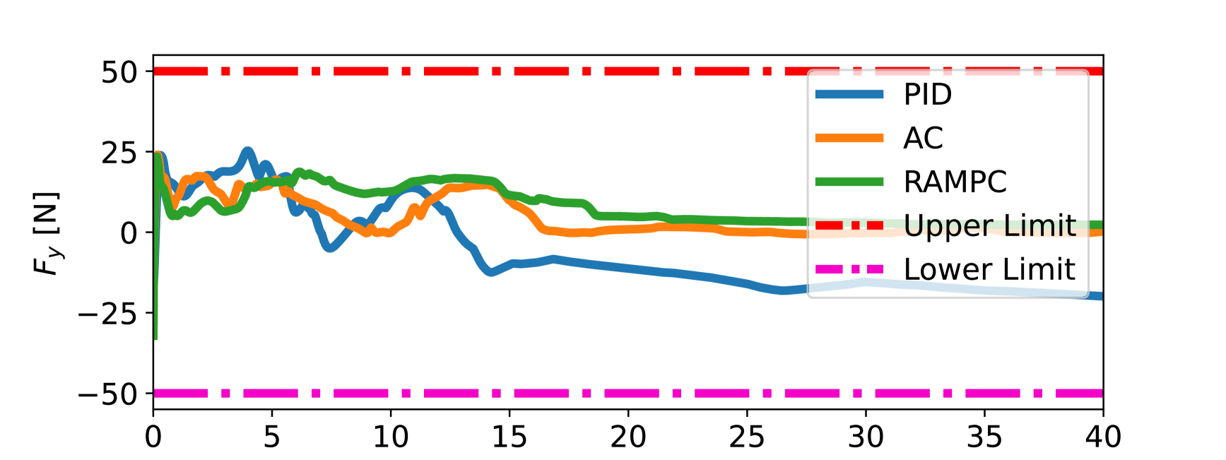
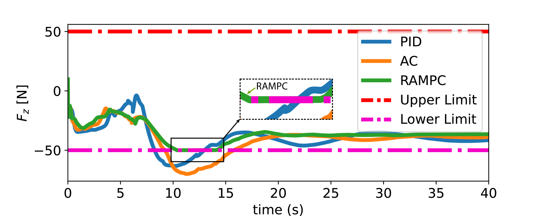
((c))

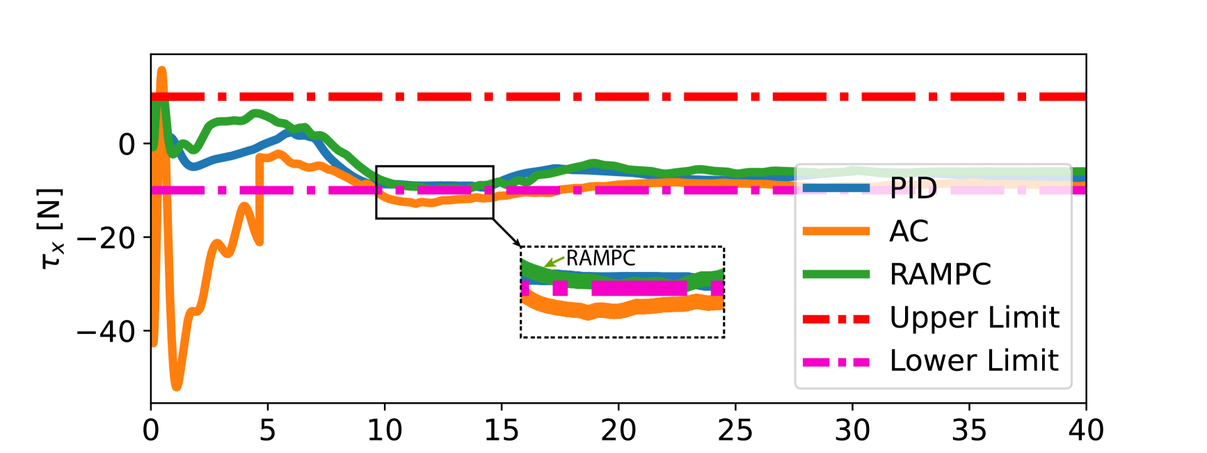
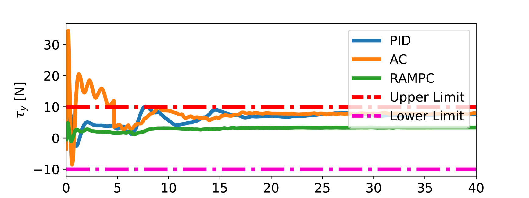
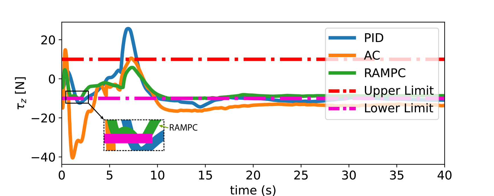
((d))

Figure 5: Exploitation results for the evolution in both states of the client in which $\theta_{k}$ in (a) and $\dot{\theta}_{k}$ in (b) and control input in which $\mathbf{f}_{k}$ in (c) and $\boldsymbol{\tau}_{k}$ in (d) compared to PID, adaptive control and robust adaptive MPC for 40 seconds.

In this section, we formulate the discrete-time linear time-varying system of the client and the performance of our robust adaptive MPC is also presented in this section with the comparison with a baseline adaptive MPC algorithm in [25]. We choose the MuJoCo [32] as our simulation platform to emulate both client and servicer in a zero-gravity environment. The parameters about the client are defined in Table. I.

The uncertainty in the parameters is described by $\mathcal{P}=\left\{\boldsymbol{\rho}_{k}\in\mathbb{R}^{3}\bigr{|}\>||\boldsymbol{\rho}_{k}||_{\infty}\leq 8\right\},$ with $\boldsymbol{\rho}^{*}_{k}=[\mathcal{K}_{k},\zeta_{k},\mathcal{D}_{k}]^{\top}$. The disturbance set is $\mathbb{W}=\left\{w\in\mathbb{R}^{3}\bigr{|}\>||w||_{\infty}\leq 0.2\right\}$ and the state and input constraints are described by

$$\mathbb{Z} =\left\{(\mathbf{x},\mathbf{u}){\in}\mathbb{R}^{2\times 6}\left|\>\begin{array}[]{rl}||\mathbf{x}[1]||\leq 0.7&,||\mathbf{x}[2]||\leq 0.2\\ \left\lVert\mathbf{u}[1,..,3]\right\rVert\leq 50&,\left\lVert\mathbf{u}[4,..,6]\right\rVert\leq 10\\ \end{array}\right.\right\}.$$

The initial state of the system is $\mathbf{x}_{0}=[0.6,0.2]^{\top}$. In both AMPC and our method, the state tube is constructed by translating and scaling the set $\mathbb{X}_{0}=\left\{\mathbf{x}\in\mathbb{R}^{2}\bigr{|}\>\left\lVert\mathbf{x}[1]\right\rVert\leq 0.8,\left\lVert\mathbf{x}[2]\right\rVert\leq 0.25\right\}$. The bounded complexity update of $\mathcal{P}_{k}$ is performed using $n_{\theta}=45$ hyperplanes which are initially chosen as outer bounds of the set $\mathcal{P}$. The cost matrices are given as

$$\begin{array}[]{l l l}\mathbf{Q}=\begin{bmatrix}1.47&0\\ 0&1.35\end{bmatrix},&\>\mathbf{R}=\begin{bmatrix}0.94&0\\ 0&1.0\end{bmatrix},&\>\boldsymbol{\Upsilon}=\begin{bmatrix}1.15&0\\ 0&1.25\end{bmatrix}.\end{array}$$

The pre-stabilizing gain used is

$$\mathbf{K}=\begin{bmatrix}-0.73&0.45\\ 0.29&0.1\end{bmatrix}.$$

The prediction horizon chosen is $N=6$ time steps for both algorithms. Both of our scheme and AMPC are initialized at $\hat{\boldsymbol{\rho}}_{0}=[0.2,0.5,2.0]^{\top}$.

Constraint Type	$\bar{\theta}$	$\underline{\theta}$	$\bar{\dot{\theta}}$	$\underline{\dot{\theta}}$	$\bar{\tau}_{i}$	$\underline{\tau_{i}}$	$\bar{f_{i}}$	$\underline{f_{i}}$
Hardware Value	1.57 rad	-1.57 rad	0.5 rad/s	-0.5 rad/s	10 N$\cdot$m	-10 N$\cdot$m	50 N	-50 N
Algorithem Value	0.3 rad	-1.2 rad	0.2 rad/s	-0.2 rad/s	2 N$\cdot$m	-2 N$\cdot$m	20 N	-20 N

Table II: Constraints for both Servicer and Client in experiments.

Fig. 5(b) and Fig. 5(b) shows the results of the state variable based on our method compared with two baseline methods. Based on the comparison results, we can see clearly that our robust adaptive MPC is not only within the safe range but also converges to be stable faster than the PID and adaptive control method.

Fig. 5(c) and Fig. 5(d) shows the results about the force and torque applied by the end-effector of the robot arm on the servicer, respectively. Based on the comparison results, we can see that the force applied based on our robust adaptive MPC algorithm is in the safe range and the magnitude of the growing speed at each time is flatter than the PID and adaptive methods which avoids the life reduction of the robot arm by excessive changes of its applied force on the EE.

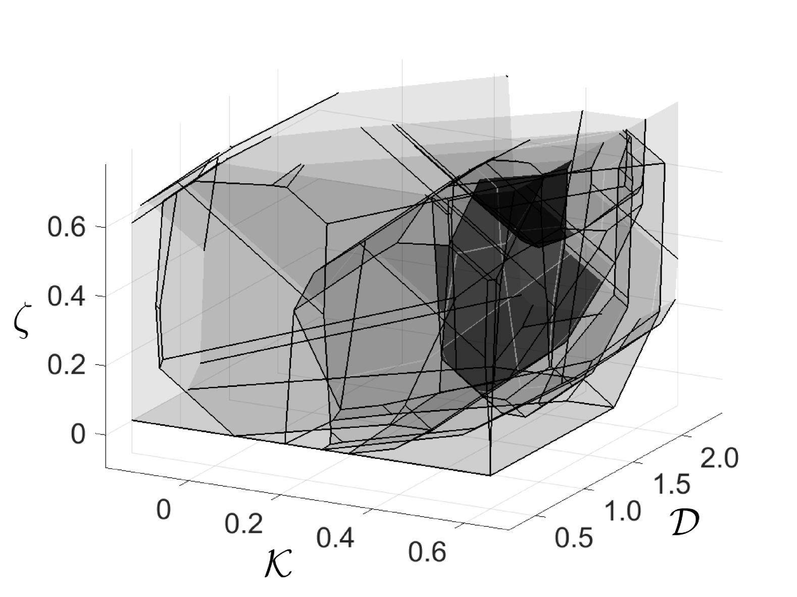
((a))

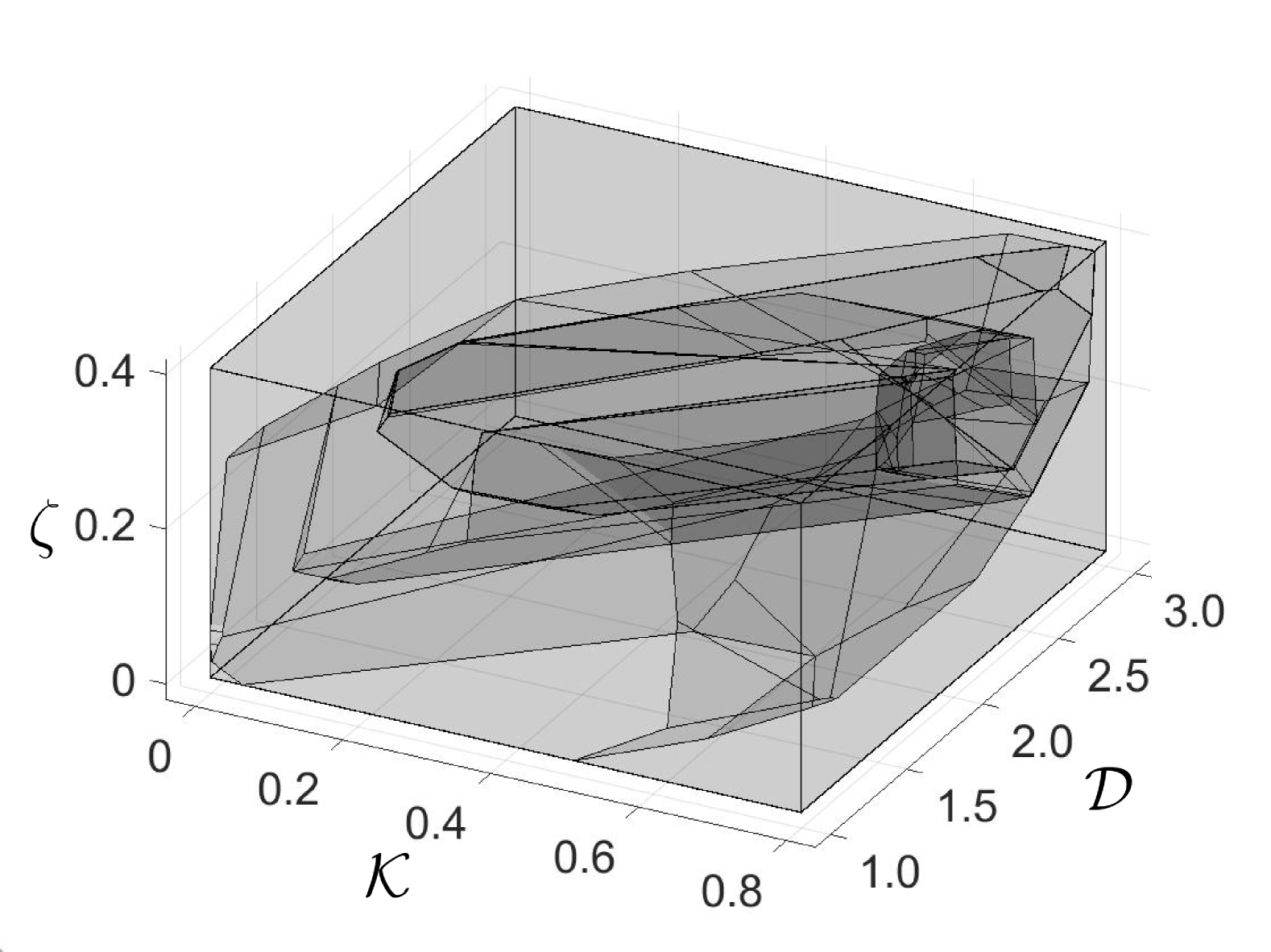
((b))

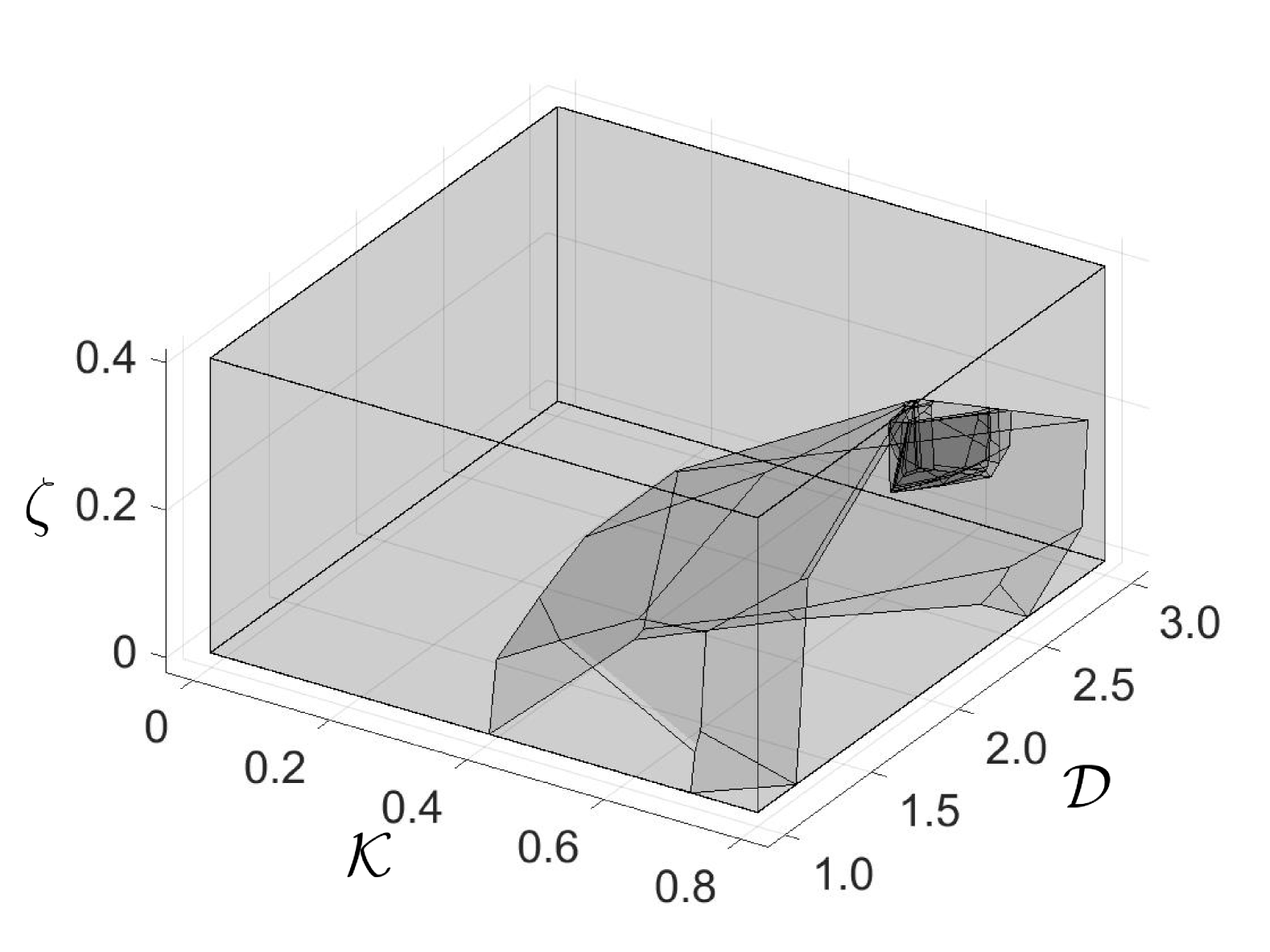
((c))

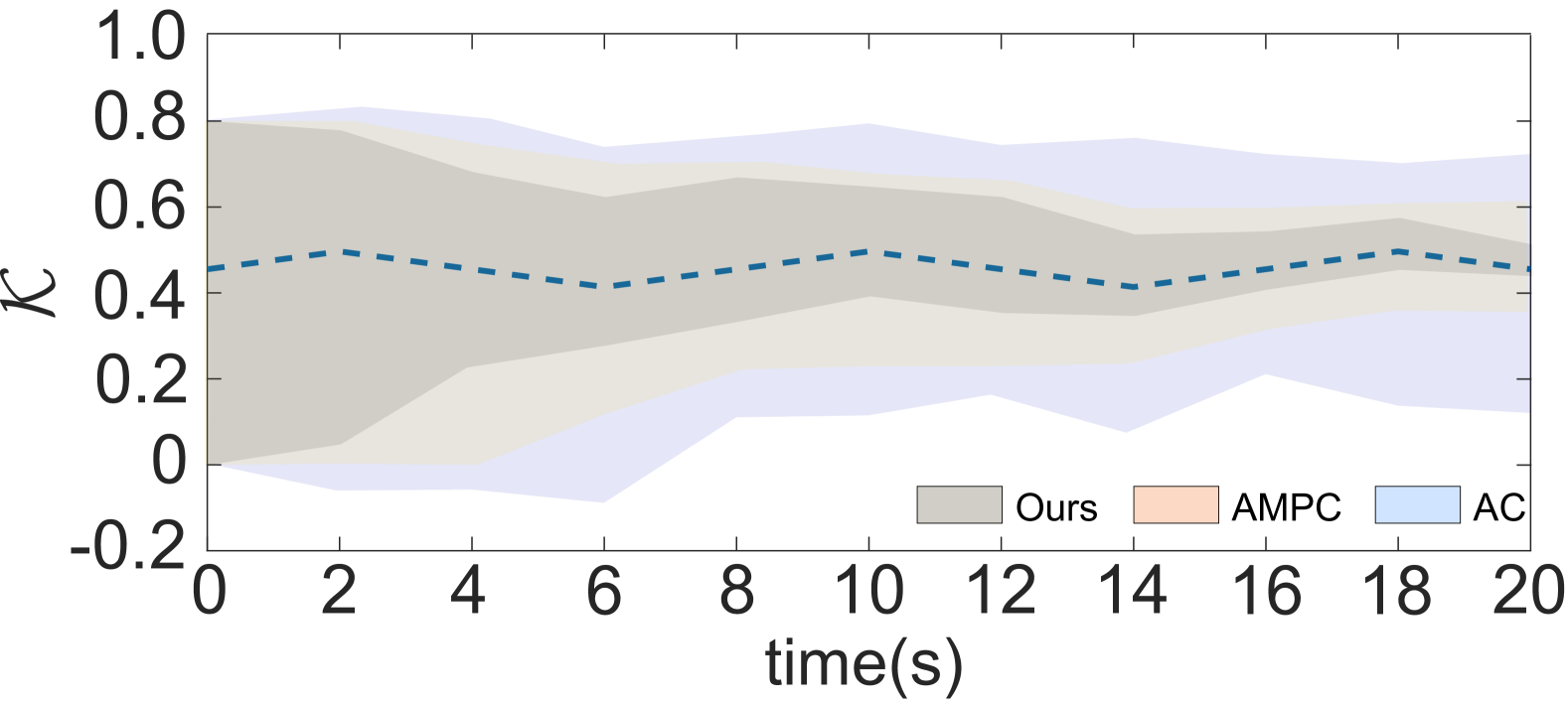
((d))

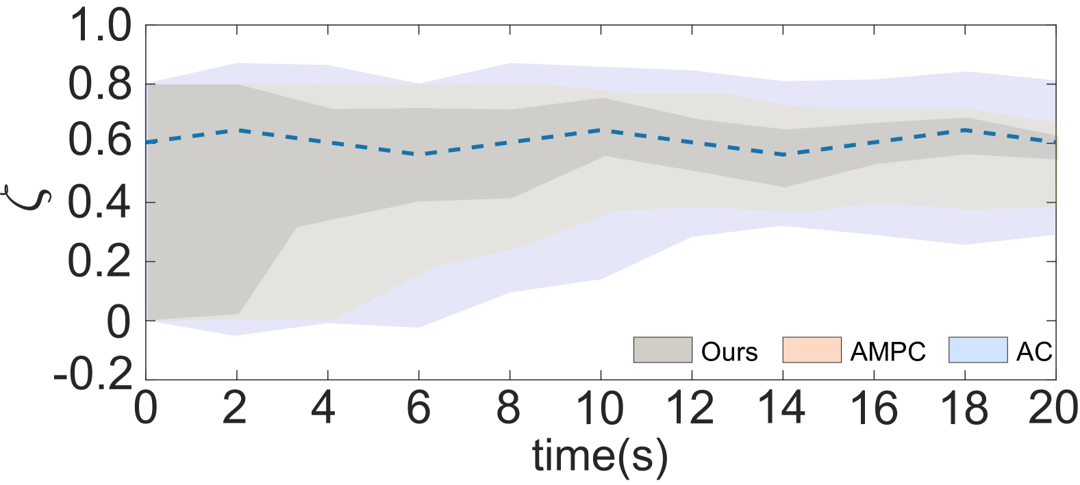
((e))

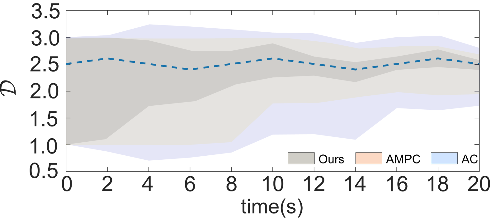
((f))

Figure 6: Exploration results for the evolution of the time-varying parameter membership set of the client during 20 seconds. (a) The polyhedron of the parameter update uses Adaptive control; (b) The polyhedron of the parameter update uses AMPC. (c) The polyhedron of the parameter update uses our Robust Adaptive MPC. (d). Comparison of time-varying parameter $\mathcal{K}$ estimation. (e). Comparison of time-varying parameter $\mathcal{\zeta}$ estimation. (f). Comparison of time-varying parameter $\mathcal{D}$ estimation.

Fig. 6(a) to Fig. 6(c) shows the results of estimating the parameter within polytope based on our method compared with two baseline methods. All parameter membership sets reduce in polygon size during the estimation process. Compare Fig. 6(a) for adaptive control based on our previous work and Fig. 6(b) for AMPC, our method results in Fig. 6(c) shows faster speed to catch the true parameter value than baseline methods. Note that the adaptation of parameters is influenced by both the initial conditions and the realization of disturbances, as the cost function does not inherently account for the benefits of future parameter learning.

Fig. 6(d) to Fig. 6(f) shows the results of each time-varying parameter estimation during the dislodging. The shadow area shows the bounded values for the estimates in each time step. Based on the result of our method compared with the two baseline methods, our method shows that it can get the true value faster, and the error is much smaller than the two baseline methods.

V Experiment Results

To prove the feasibility of our robust adaptive MPC in hardware, we also implement our robust adaptive MPC in our testbed compared with PID and adaptive control, as shown in Fig. 7. We leverage the testbed in our lab to build up the dislodging environment in space but consider the gravity based on the limitation. We use UR5e to emulate a Servicer that can apply 6 DoF wrench in SE(3). Also, we use the WAM robot arm to hold the satellite module, the details of which are shown on the right-bottom side, to emulate a Client, which is a free-flying spacecraft that can decouple the dynamics from the Servicer during dislodging. For both Client and Servicer, we set up two types of safety constraints in our algorithm as shown in Table. II based on the hardware limitation to ensure the dislodging can proceed well as shown in Fig. 8a; once either is out of its hardware constraints based on the value in Table. II, the system will stop to denote the potential risk occurrence during the dislodging as shown in Fig. 8b. Note that to compare and discover the performance with different methods, we set up a scheme in our program that if any variable’s value shown in Table II is between the hardware constraints and software constraints, the robot system can still work but denote the potential damage will happen to simulate the real scenarios in space. The hinge’s top-side view during dislodging is shown in Fig. 9. All the safe constraints we set up in our program are under the real constraints for both Client and Servicer to avoid any danger happening on the hardware.

Fig. 10 shows the wrench applied by the Client during the dislodging using PID control method. Based on the results, we can see clearly that the PID method can make the Client out of its safe range easily, which will break the hardware easily.

Fig. 11 shows the wrench applied by the Client during the dislodging via adaptive control. Based on the results, it’s also straightforward to see that even though the adaptive control method shows a little bit better than PID, it still can make the Client be out of its safe range to bring the potential breakage for the hardware.

Fig. 12 shows the wrench applied by the Client during the dislodging via our robust adaptive MPC. Based on the results, we can find that the adaptive control method can ensure the wrench from the Client is always under the constraint to keep the safe during dislodging.

Fig. 13 shows the comparison results for the angular velocity, angle position and tracking error during dislodging. We can clearly see that our robust adaptive MPC shows good performance in terms of both convergence speed and constraint limits.

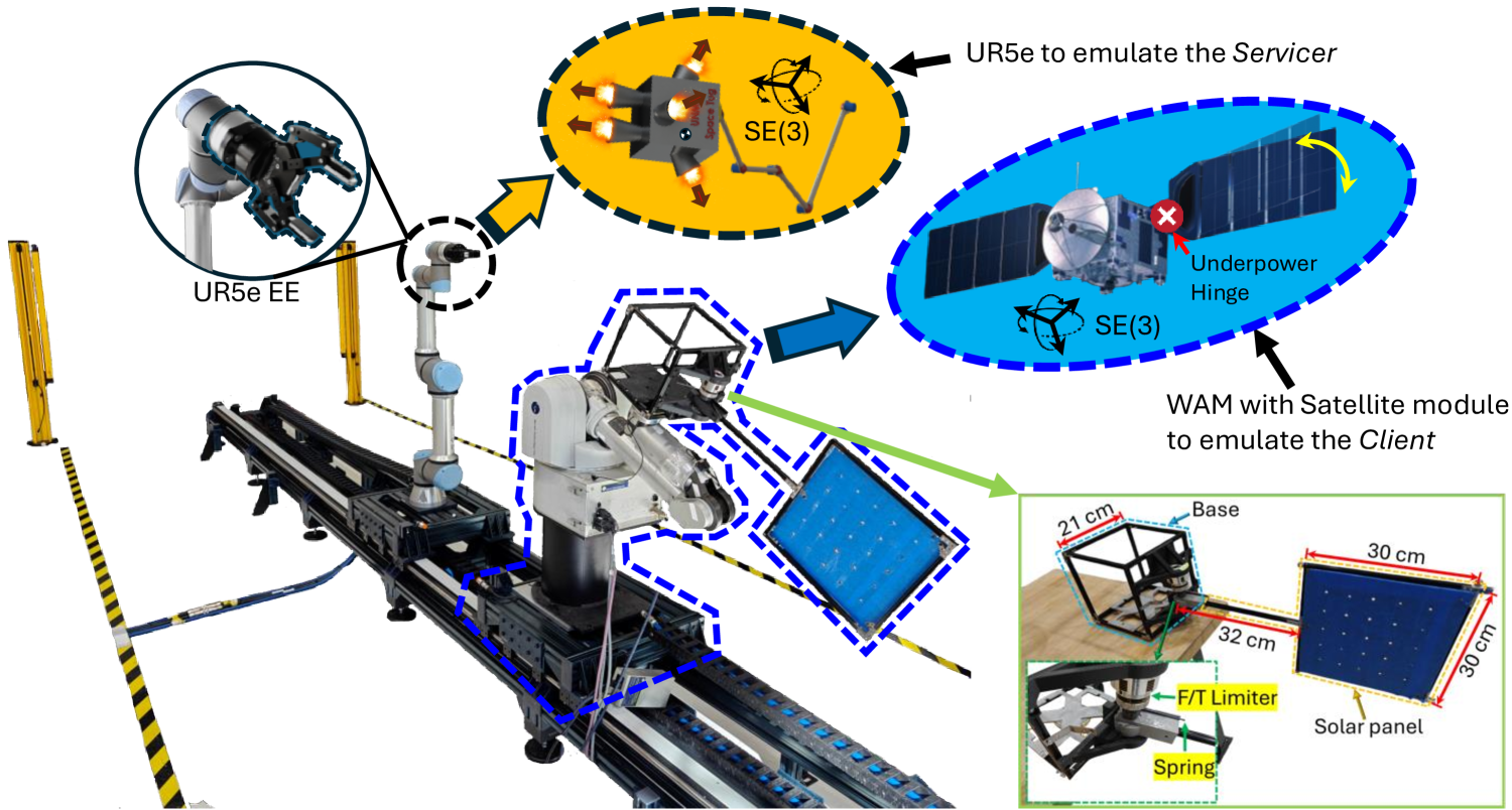
Figure 7: The whole hardware setup for experiment. We use UR5e and WAM robot with gantry system to emulate the servicer and client, respectively. The detail of the satellite module design shown on the left-bottom side.

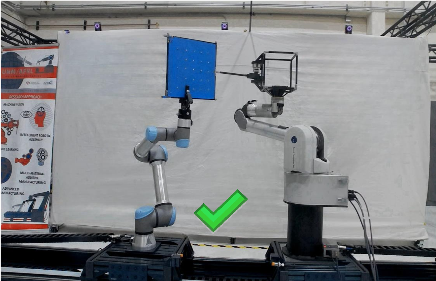
((a))

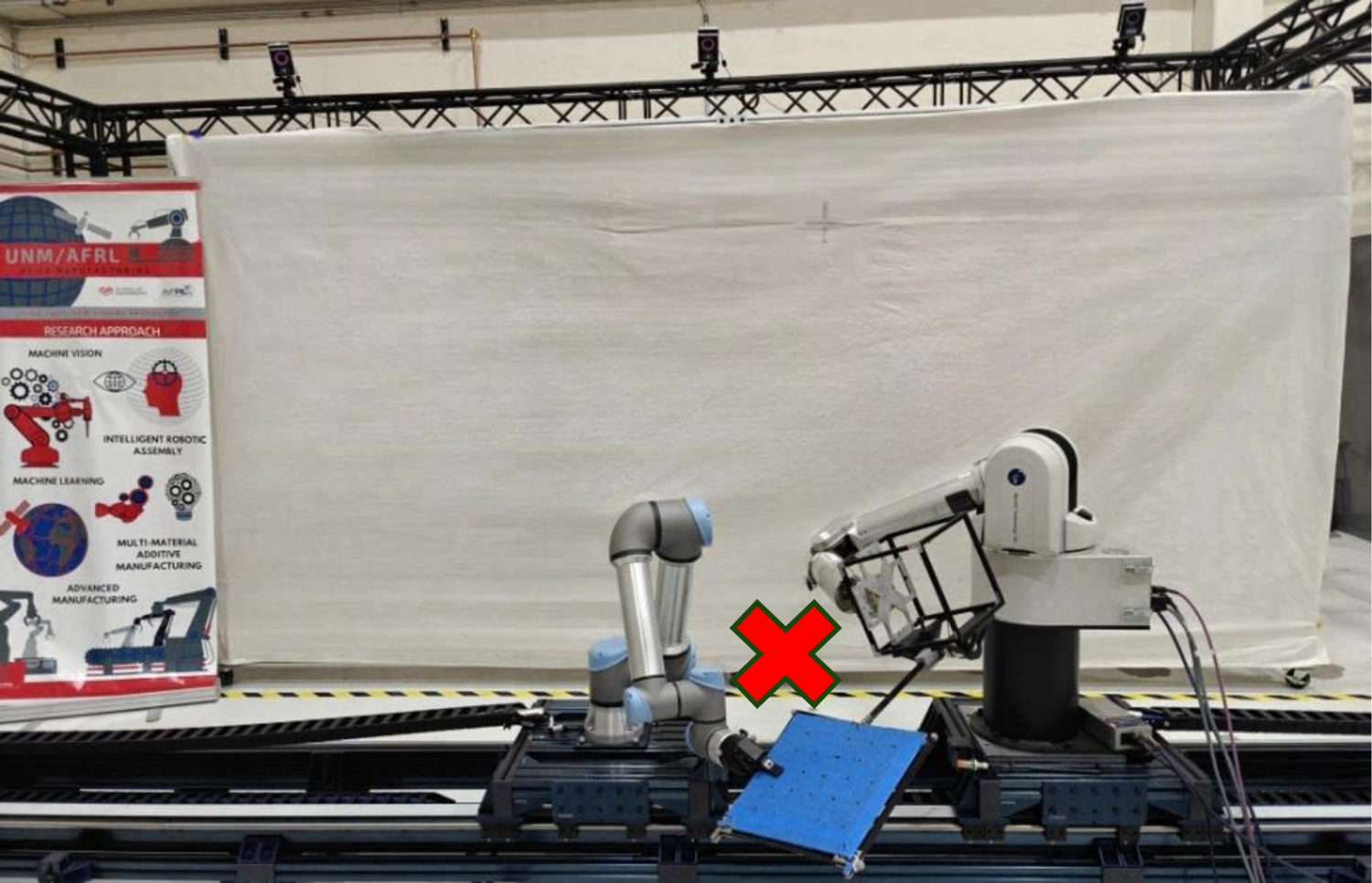
((b))

Figure 8: Hardware status during the dislodging. (a) shows the normal status during the dislodging that both Client and Servicer are in safe range. (b) shows the failure of dislodging that either is out of its safe range based on the hardware constraints in Table.II.

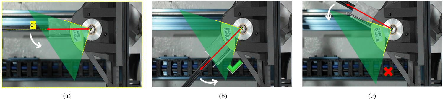
Figure 9: Top-view of the hinge during the dislodging. The green region shows the safe dislodging range of the hinge’s rotation. (a) shows the initial position of the hinge before the dislodging. (b) shows the hinge is in the safe range. (c) shows the hinge is out of the safe range.

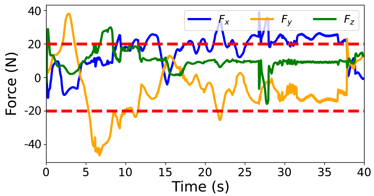
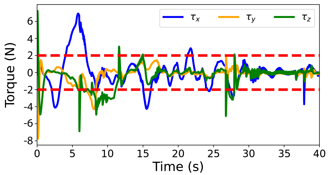
((a))

((b))

Figure 10: Force and torque applied by the EE of UR5e during the dislodging via PID.

VI Conclusions

In this paper, we presented a novel, robust adaptive MPC algorithm via set-membership in time-varying parameter estimation during the dislodging task. The algorithm employs an online set-membership identification technique to progressively minimize time-varying parameter uncertainty while utilizing a tube-based MPC strategy to guarantee robust compliance with system constraints. A predicted state tube is leveraged to account for the influence of future control inputs on the identification process while optimizing the anticipated worst-case cost. We compare our scheme with a state-of-the-art adaptive MPC algorithm and prove that our algorithm shows better performance in both parameter estimation and calculation speed during the manipulation process. In our future research, we will integrate related learning methods based on our robust adaptive MPC algorithm to improve the model accuracy with data-driven system identification.

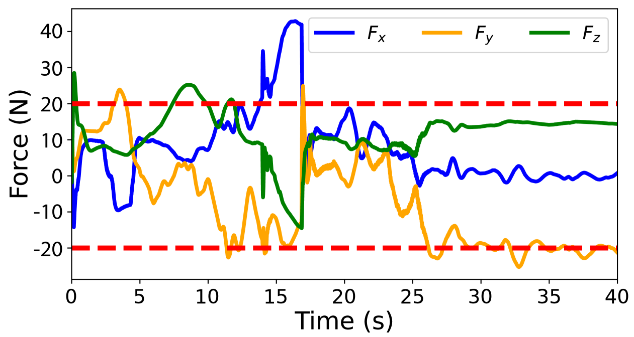
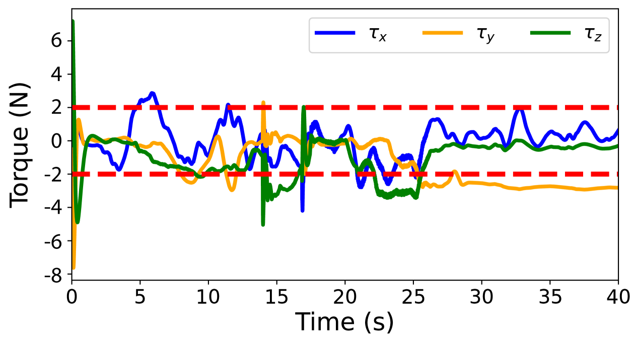
((a))

((b))

Figure 11: Force and torque applied by the EE of UR5e during the dislodging via Adaptive Control.

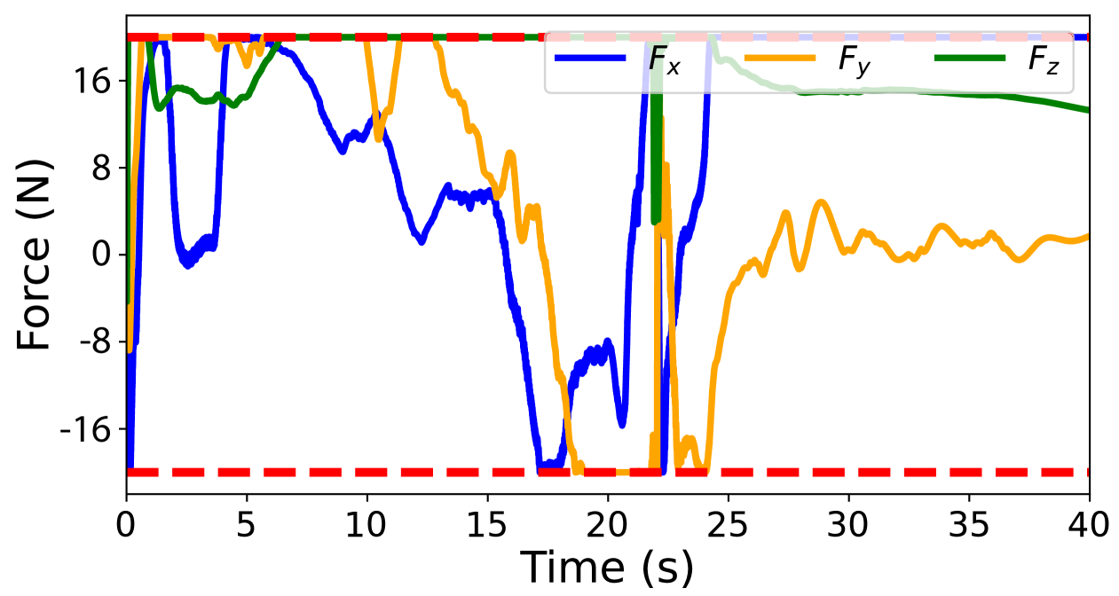
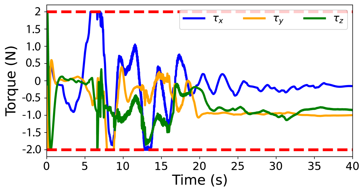
((a))

((b))

Figure 12: Force and torque applied by the EE of UR5e during the dislodging via robust adaptive MPC.

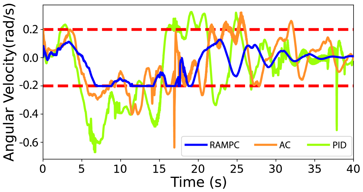
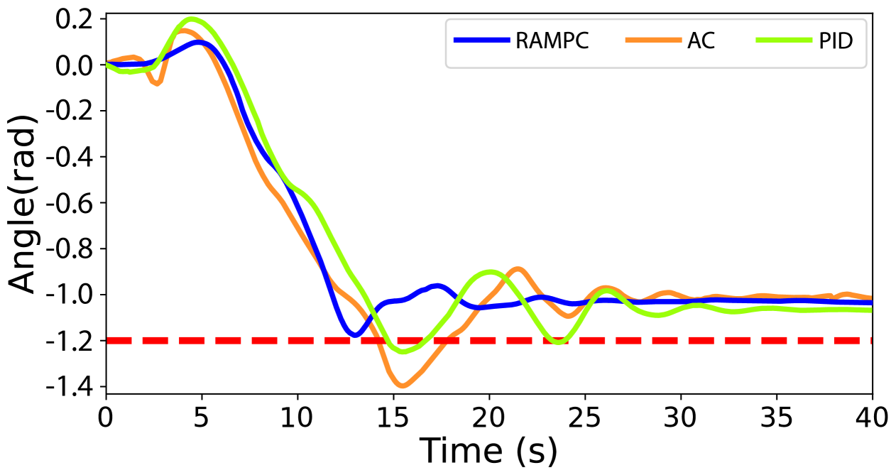
((a))

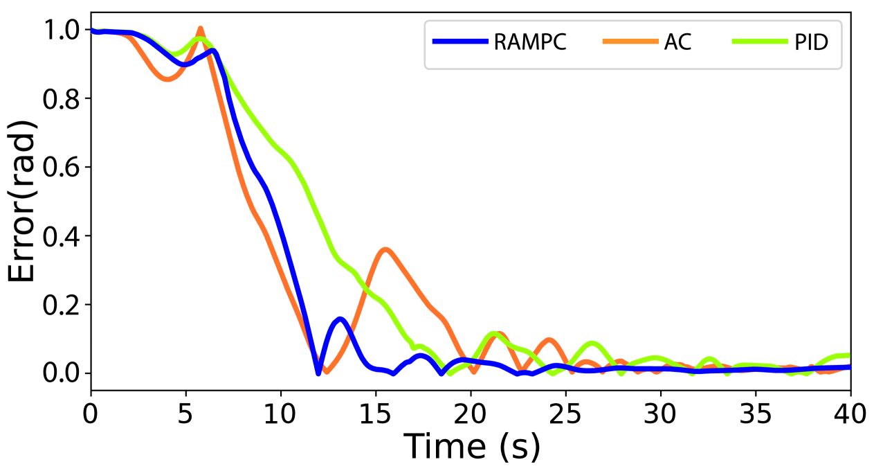
((b))

((c))

Figure 13: Angular states-angular velocity (a) and dislodged angle (b) and tracking error during the dislodging via three methods.

References

- [1] E. M. Emme, “Part ii: Early history of the space age,” Aerospace Historian, vol. 13, no. 3, pp. 127–132, 1966.
- [2] M. Tafazoli, “A study of on-orbit spacecraft failures,” Acta Astronautica, vol. 64, no. 2-3, pp. 195–205, 2009.
- [3] A. Flores-Abad, O. Ma, K. Pham, and S. Ulrich, “A review of space robotics technologies for on-orbit servicing,” Progress in aerospace sciences, vol. 68, pp. 1–26, 2014.
- [4] M. Luu and D. E. Hastings, “Review of on-orbit servicing considerations for low-earth orbit constellations,” ASCEND 2021, p. 4207, 2021.
- [5] J. P. Davis, J. P. Mayberry, and J. P. Penn, “On-orbit servicing: Inspection repair refuel upgrade and assembly of satellites in space,” The Aerospace Corporation, report, p. 25, 2019.
- [6] C. Oestreich, A. T. Espinoza, J. Todd, K. Albee, and R. Linares, “On-orbit inspection of an unknown, tumbling target using nasa’s astrobee robotic free-flyers,” in Proceedings of the IEEE/CVF Conference on Computer Vision and Pattern Recognition, pp. 2039–2047, 2021.
- [7] J. Virgili-Llop, C. Zagaris, R. Zappulla, A. Bradstreet, and M. Romano, “A convex-programming-based guidance algorithm to capture a tumbling object on orbit using a spacecraft equipped with a robotic manipulator,” The International Journal of Robotics Research, vol. 38, no. 1, pp. 40–72, 2019.
- [8] D. Parikh, D. van Wijk, and M. Majji, “Safe multi-agent satellite servicing with control barrier functions,” arXiv preprint arXiv:2502.10480, 2025.
- [9] P. Boning and S. Dubowsky, “Identification of actuation efforts using limited sensory information for space robots,” in Proceedings 2006 IEEE International Conference on Robotics and Automation, 2006. ICRA 2006., pp. 3873–3878, IEEE, 2006.
- [10] Z. Ma and G. Sun, “Adaptive sliding mode control of tethered satellite deployment with input limitation,” Acta Astronautica, vol. 127, pp. 67–75, 2016.
- [11] G. Beaumet, G. Verfaillie, and M.-C. Charmeau, “Feasibility of autonomous decision making on board an agile earth-observing satellite,” Computational Intelligence, vol. 27, no. 1, pp. 123–139, 2011.
- [12] E. Laing, P. Ashley, F. B. Naini, and D. S. Gill, “Space maintenance,” International journal of paediatric dentistry, vol. 19, no. 3, pp. 155–162, 2009.
- [13] A. Rivera and A. Stewart, “Study of spacecraft deployables failures,” in 19th European Space Mechanisms and Tribology Symposium (ESMATS) 2021, 2021.
- [14] N. J. S. Center, “50 years ago: Skylab 2 astronauts deploy jammed solar array during spacewalk,” 2023.
- [15] K. Higuchi, M. Natori, and M. Abe, “Unexpected behavior of a flexible solar array at retraction under microgravity,” Acta Astronautica, vol. 50, no. 11, pp. 681–689, 2002.
- [16] G. A. Landis, “Space photovoltaics for extreme high-temperature missions,” in Photovoltaics for Space, pp. 393–410, Elsevier, 2023.
- [17] L. Gao, G. Cordova, C. Danielson, and R. Fierro, “Autonomous multi-robot servicing for spacecraft operation extension,” in 2023 IEEE/RSJ International Conference on Intelligent Robots and Systems (IROS), pp. 10729–10735, IEEE, 2023.
- [18] Y. Xu, H.-Y. Shum, J.-J. Lee, and T. Kanade, “Adaptive control of space robot system with an attitude controlled base,” Space robotics: Dynamics and control, pp. 229–268, 1993.
- [19] S. Ulrich and J. Z. Sasiadek, “Modified simple adaptive control for a two-link space robot,” in Proceedings of the 2010 American Control Conference, pp. 3654–3659, IEEE, 2010.
- [20] Z.-w. Yu and G.-p. Cai, “Robust adaptive control of a 6-dof space robot with flexible panels,” International Journal of Dynamics and Control, vol. 7, no. 4, pp. 1370–1378, 2019.
- [21] N. T. Nguyen and N. T. Nguyen, Model-reference adaptive control. Springer, 2018.
- [22] H. Enomoto, M. Ishige, T. Umedachi, M. Kamezaki, and Y. Kawahara, “Delicate jamming grasp: Detecting deformation of fragile objects using permanent magnet elastomer membrane,” IEEE Robotics and Automation Letters, 2023.
- [23] M. Lorenzen, F. Allgöwer, and M. Cannon, “Adaptive model predictive control with robust constraint satisfaction,” IFAC-PapersOnLine, vol. 50, no. 1, pp. 3313–3318, 2017.
- [24] J. Köhler, P. Kötting, R. Soloperto, F. Allgöwer, and M. A. Müller, “A robust adaptive model predictive control framework for nonlinear uncertain systems,” International Journal of Robust and Nonlinear Control, vol. 31, no. 18, pp. 8725–8749, 2021.
- [25] A. Aboudonia and J. Lygeros, “Adaptive learning-based model predictive control for uncertain interconnected systems: A set membership identification approach,” arXiv preprint arXiv:2404.16514, 2024.
- [26] K. Wesselowski and R. Fierro, “A dual-mode model predictive controller for robot formations,” in 42nd IEEE International Conference on Decision and Control (IEEE Cat. No. 03CH37475), vol. 4, pp. 3615–3620, IEEE, 2003.
- [27] A. C. Tribble, The space environment: implications for spacecraft design-revised and expanded edition. Princeton University Press, 2020.
- [28] H. Fang, E. Im, J. Lin, and S. Scarborough, “Shape memory composite hybrid hinge,” tech. rep., 2012.
- [29] B. T. Lopez, J.-J. E. Slotine, and J. P. How, “Dynamic tube mpc for nonlinear systems,” in 2019 American Control Conference (ACC), pp. 1655–1662, IEEE, 2019.
- [30] Y. Wang, L. Xie, and C. E. De Souza, “Robust control of a class of uncertain nonlinear systems,” Systems & control letters, vol. 19, no. 2, pp. 139–149, 1992.
- [31] B. Kouvaritakis and M. Cannon, “Model predictive control,” Switzerland: Springer International Publishing, vol. 38, pp. 13–56, 2016.
- [32] E. Todorov, T. Erez, and Y. Tassa, “Mujoco: A physics engine for model-based control,” in 2012 IEEE/RSJ international conference on intelligent robots and systems, pp. 5026–5033, IEEE, 2012.