Non-Lorentzian model for strong exciton-plasmon coupling

Abstract

We develop a non-Lorentzian approach for quantum emitters (QE) resonantly coupled to localized surface plasmons (LSP) in metal-dielectric structures. Using the exact LSP Green function, we derive non-Lorentzian version of Maxwell-Bloch equations which describe LSP in terms of metal complex dielectric function rather than via Lorentzian resonances. For a single QE coupled to the LSP, we obtain an explicit expression for the system effective optical polarizability which, in the Lorentzian approximation, recovers the classical coupled oscillator (CO) model. We demonstrate that non-Lorentzian effects originating from the temporal dispersion of metal dielectric function affect dramatically the optical spectra as the system transitions to the strong coupling regime. Specifically, in contrast to Lorentzian models, the main spectral weight is shifted towards the lower energy polaritonic band, consistent with the experiment.

I Introduction

The effects of strong coupling between localized surface plasmons (LSP) in metal-dielectric structures and quantum emitters (QE) such as excitons in semiconductors or dye molecules have recently attracted considerable interest driven by numerous potential applications including ultrafast reversible switching [1, 2, 3], quantum computing [4, 5] or light harvesting [6]. In the strong coupling regime, coherent energy exchange between QEs and LSP [7, 8] leads to the emergence of mixed polaritonic states with energy bands separated by the anticrossing gap (Rabi splitting) [9]. While Rabi splittings in the emission spectra of excitons coupled to cavity modes in semiconductor microcavities are about several meV [10, 11, 12], they can reach hundreds meV in hybrid plasmonic systems involving excitons in J-aggregates [13, 14, 15, 16, 17, 18, 19, 20], in various dye molecules [21, 22, 23, 24, 25] or in semiconductor nanostructures [26, 27, 28, 29] resonantly coupled to LSPs. For single QEs, however, reaching a strong coupling regime is a challenging task as it requires extremely small LSP mode volumes available mainly in nanogaps [30, 31, 32].

At the same time, the exact shape of optical spectra is determined by several competing processes and has been a subject of active debate [36, 37, 38, 39, 40, 41, 42, 43, 45, 44, 46, 47, 48]. In general, the scattering cross-section for a nanoscale system characterized by a localized dipole moment is proportional to $\omega^{4}$ [9], where $\omega$ is the incident light frequency, implying that, in the strong coupling regime, the upper energy polaritonic band should be relatively enhanced. Such a spectral profile is due to a faster dipole radiation rate at higher frequencies $\gamma^{rad}\propto\omega^{3}$, as described. e.g., by the widely-used classical model of two coupled oscillators (CO) [33, 34, 35]. In this model, only one of the oscillators (LSP) couples to the radiation field while QE’s coupling to the radiation is neglected due to its much smaller optical dipole moment. However, recent experiments for excitons resonantly coupled to cavity modes in semiconductor microcavities [36, 37, 38] or to LSPs in metal-dielectric structures [39, 41, 42, 40, 31] reveal the opposite spectral asymmetry pattern with a visible enhancement of the lower energy polaritonic band. For plasmonic systems, such a shift of the spectral weight towards the lower energy band may arise from Fano interference between LSP’s and LSP-induced QE’s dipole moments [45, 46, 47, 48]. Note, however, that due to a much smaller QE dipole moment, a significant interference effect would require either an extremely strong field confinement [45, 46, 47] or a large number of QEs strongly coupled to the LSP [48].

On the other hand, for molecular excitons coupled to a cavity mode, the accurate spectral weight of polaritonic bands in the emission spectra is obtained by incorporating excitations of vibronic modes within quantum master equation approach, [43, 44]. For plasmonic systems characterized by a frequency-dependent complex dielectric function $\varepsilon(\omega)=\varepsilon^{\prime}(\omega)+i\varepsilon^{\prime\prime}(\omega)$ of host metal, the emission spectra with accurate spectral weight distribution have been obtained [49] within macroscopic quantum electrodynamics approach [50, 51], adopted to metal-dielectric structures supporting LSPs [52], by accounting for temporal dispersion in the LSP optical dipole moment. However, such quantum approaches require extensive numerical efforts and therefore are not easily suitable for modeling of experimental optical spectra.

In this paper we present a semiclassical model that fully accounts for temporal dispersion and losses in the metal, encoded in $\varepsilon(\omega)$, and the interference effects for QEs resonantly coupled to LSP. Using our recent results for the LSP Green function [53], we develop non-Lorentzian extension of Maxwell-Bloch equations where LSP is described in terms of metal dielectric function rather than by Lorentzian resonances. For a metal nanoparticle (NP) of arbitrary shape interacting with a QE, we obtain the system effective optical polarizability, which, in the in the Lorentzian approximation, recovers the CO model results. By comparing the optical spectra obtained with our non-Lorentzian model and its Lorentzian approximation (CO model), we observe spectral weight shift towards the lower energy polaritonic band, consistent with the experiment, and trace its origin to frequency dependence of the metal dielectric function which is neglected in the CO model. Our analytical model can be used for accurate description of experimental spectra of strongly-coupled exciton-plasmon hybrid systems without any significant numerical effort.

The paper is organized as follows. In Sec. II we outline our non-Lorentzian approach to the LSP Green funnction and optical polarizability of plasmonic NP. In Sec. III, we derive non-Lorentzian Maxwell-Bloch equations for QEs resonantly coupled to the LSP in a metal-dielectric structure. In Sec. IV, we obtain the effective polarizability for a QE strongly coupled to the LSP and show that, in the Lorentzian approximation, it reduces to the CO model results. In Sec. V, we present our numerical results for optical spectra of the QE-LSP system in the strong coupling regime. Section VI concludes the paper.

II Non-Lorentzian approach to localized surface plasmons

II.1 Plasmon modes and the Green’s function

Here, we outline our approach to the LSP Green function [53] we rely upon in the following sections for developing non-Lorentzian model for strongly coupled QE-LSP system. We consider a metal-dielectric structure supporting LSP excitations with discrete frequencies $\omega_{n}$ which are localized at a length scale much smaller than the radiation wavelength. Each system region of volume $V_{i}$, metallic or dielectric, is characterized by dielectric function $\varepsilon_{i}(\omega)$, so that the full dielectric function is $\varepsilon(\omega,\bm{r})=\sum_{i}\theta_{i}(\bm{r})\varepsilon_{i}(\omega)$, where $\theta_{i}(\bm{r})$ is the unit step function that vanishes outside $V_{i}$. We assume that dielectric regions’ permittivities $\varepsilon_{i}$ are constants, and for the metallic region we adopt complex dielectric function $\varepsilon(\omega)=\varepsilon^{\prime}(\omega)+i\varepsilon^{\prime\prime}(\omega)$. In the absence of retardation effects, the LSP modes are defined by the lossless Gauss equation as [54]

$$\bm{\nabla}\cdot\left[\varepsilon^{\prime}(\omega_{n},\bm{r})\bm{\nabla}\Phi_{n}(\bm{r})\right]=0,$$ (1)

where $\Phi_{n}(\bm{r})$ and $\bm{E}_{n}(\bm{r})=-\bm{\nabla}\Phi_{n}(\bm{r})$ are, respectively, the potential and electric field of LSP mode $\omega_{n}$, which we chose real. Note that LSP eigenmodes are orthogonal in each region: $\int\!dV_{i}\bm{E}_{n}(\bm{r})\cdot\bm{E}_{n^{\prime}}(\bm{r})=\delta_{nn^{\prime}}\!\int\!dV_{i}\bm{E}_{n}^{2}(\bm{r})$.

In the presence of metal-dielectric structure, the EM dyadic Green’s function $\bm{D}(\omega;\bm{r},\bm{r}^{\prime})$ satisfies (in the operator form) $\bm{\nabla}\!\times\!\bm{\nabla}\!\times\bm{D}-(\omega^{2}/c^{2})\varepsilon\bm{D}=(4\pi\omega^{2}/c^{2})\bm{I}$, where $\bm{I}$ is the unit tensor. In the near field, we are interested in the longitudinal part of $\bm{D}$, which is obtained by applying the operator $\bm{\nabla}$ to both sides. In the quasistatic case, the dyadic Green function $\bm{D}(\omega;\bm{r},\bm{r}^{\prime})$ is related to scalar Green’s function for the potentials $D(\omega;\bm{r},\bm{r}^{\prime})$ as $\bm{D}(\omega;\bm{r},\bm{r}^{\prime})=\bm{\nabla}\bm{\nabla}^{\prime}D(\omega;\bm{r},\bm{r}^{\prime})$. The latter satisfies equation [compare to Eq. (1)]

$$\bm{\nabla}\cdot\left[\varepsilon(\omega,\bm{r})\bm{\nabla}D(\omega;\bm{r},\bm{r}^{\prime})\right]=4\pi\delta(\bm{r}-\bm{r}^{\prime}).$$ (2)

An explicit expression for the scalar Green function is found by adopting decomposition $D=D_{0}+D_{\rm LSP}$, where $D_{0}(\bm{r}-\bm{r}^{\prime})=-|\bm{r}-\bm{r}^{\prime}|^{-1}$ is the free-space Green’s function and $D_{\rm LSP}(\omega;\bm{r},\bm{r}^{\prime})$ is the LSP contribution. Expanding that latter over the eigenmodes of Eq. (1), we obtain

$$D_{\rm LSP}(\omega;\bm{r},\bm{r}^{\prime})=\sum_{n}D_{n}(\omega)\Phi_{n}(\bm{r})\Phi_{n}(\bm{r}^{\prime}),$$ (3)

where coefficients $D_{n}(\omega)$ have non-Lorentzian form [53]

$$D_{n}(\omega)=\dfrac{4\pi}{\int\!dV_{\rm m}\bm{E}_{n}^{2}}\frac{1}{\varepsilon^{\prime}(\omega_{n})-\varepsilon(\omega)}.$$ (4)

Here, integration takes place over the metal volume $V_{m}$. Although the expansion in Eq. (3) involves eigenmodes of the lossless Gauss equation (1), the coefficients $D_{n}$ are defined by complex dielectric function $\varepsilon(\omega,\bm{r})$. While Eq. (4) does not depend explicitly on (constant) dielectric permittivities, the latter enter indirectly through LSP frequencies $\omega_{n}$.

Accordingly, the non-Lorentzian dyadic Green’s function is $\bm{D}_{\rm LSP}(\omega;\bm{r},\bm{r}^{\prime})=\sum_{n}D_{n}(\omega)\bm{E}_{n}(\bm{r})\bm{E}_{n}(\bm{r}^{\prime})$. In the Lorentzian approximation, using the Gauss equation (1) in the integral form $\int\!dV\varepsilon^{\prime}(\omega_{n},\bm{r})\bm{E}_{n}^{2}(\bm{r})=0$, the dielectric function $\varepsilon(\omega)$ in Eq. (4) is expanded near the LSP frequencies $\omega_{n}$ as

$$\varepsilon(\omega)=(\omega-\omega_{n})\varepsilon^{\prime}_{n}+i\varepsilon^{\prime\prime}(\omega_{n}),$$ (5)

where we denoted $\varepsilon^{\prime}_{n}\equiv\partial\varepsilon^{\prime}(\omega_{n})/\partial\omega_{n}$. The Lorentzian LSP Green function has the form [55, 56]

$$\bm{D}_{\rm LSP}^{L}(\omega;\bm{r},\bm{r}^{\prime})=\sum_{n}\frac{\omega_{n}}{4U_{n}}\frac{\bm{E}_{n}(\bm{r})\bm{E}_{n}(\bm{r}^{\prime})}{\omega_{n}-\omega-i\gamma_{n}/2},$$ (6)

where

$$U_{n}=\frac{1}{16\pi}\int\!dV\frac{\partial[\omega_{n}\varepsilon^{\prime}(\omega,\bm{r})]}{\partial\omega_{n}}\bm{E}_{n}^{2}=\frac{\omega_{n}\varepsilon^{\prime}_{n}}{16\pi}\int\!dV_{\rm m}\bm{E}_{n}^{2}$$ (7)

is the LSP mode energy and $\gamma_{n}=2\varepsilon^{\prime\prime}(\omega_{n})/\varepsilon^{\prime}_{n}$ is the LSP decay rate [54].

The Gauss equation (1) does not specify the LSP mode field’s overall normalization. The normalized LSP mode field $\tilde{\bm{E}}_{n}$ is determined by matching the LSP radiative decay rate with the decay rate $\gamma_{n}^{rad}=4\bm{\mu}_{n}^{2}\omega_{n}^{3}/3\hbar c^{3}$ of a localized dipole with excitation frequency $\omega_{n}$ and optical dipole moment $\bm{\mu}_{n}=\!\int\!dV\chi^{\prime}(\omega_{n},\bm{r})\tilde{\bm{E}}_{n}(\bm{r})$. We obtain

$$\tilde{\bm{E}}_{n}(\bm{r})=\frac{1}{2}\sqrt{\frac{\hbar\omega_{n}}{U_{n}}}\,\bm{E}_{n}(\bm{r})=\sqrt{\frac{4\pi\hbar}{\varepsilon^{\prime}_{n}}}\dfrac{\bm{E}_{n}(\bm{r})}{\left(\int\!dV_{\rm m}\bm{E}_{n}^{2}\right)^{1/2}},$$ (8)

where $\chi=(\varepsilon-1)/4\pi$ is susceptibility and $c$ is the speed of light. The normalization factor reflects conversion of the photon energy $\hbar\omega_{n}$ into LSP energy $U_{n}$.

Finally, the non-Lorentzian LSP Green function takes the form $\bm{D}_{\rm LSP}(\omega;\bm{r},\bm{r}^{\prime})=\sum_{n}\bm{D}_{n}(\omega;\bm{r},\bm{r}^{\prime})$, where

$$\bm{D}_{n}(\omega;\bm{r},\bm{r}^{\prime})=\sum_{n}\dfrac{\varepsilon^{\prime}_{n}}{\hbar}\frac{\tilde{\bm{E}}_{n}(\bm{r})\tilde{\bm{E}}_{n}(\bm{r}^{\prime})}{\varepsilon^{\prime}(\omega_{n})-\varepsilon(\omega)},$$ (9)

which implies a straightforward Lorentzian limit as $\varepsilon^{\prime}_{n}$ cancels out the LSP pole residue. We stress that, in contrast to the Lorentzian approximation (6), the non-Lorentzian LSP Green function (9) is exact for the quasistatic case. Although the above expression for $\bm{D}_{\rm LSP}$ does not explicitly depend on dielectric permittivities $\varepsilon_{i}$, the latter enter though boundary conditions for mode field and LSP frequency.

II.2 Optical polarizability of metal nanoparticles

In the following, we consider binary systems, i.e., metal nanostructures in dielectric medium with permittivity $\varepsilon_{d}$ and set $\varepsilon_{d}=1$ for now.

With help of the LSP Green function (9), a simple expression for optical polarizability of a small NPs of arbitrary shape can be obtained [53]. In the following, we consider binary systems, i.e., metal NPs in a dielectric medium with permittivity $\varepsilon_{d}$ and set $\varepsilon_{d}=1$ for now. In the presence of incident field $\bm{E}_{0}e^{-i\omega t}$, the field inside the metal is $\bm{E}(\omega,\bm{r})=\bm{E}_{0}+\bm{E}_{\rm LSP}(\omega,\bm{r})$, where $\bm{E}_{\rm LSP}(\omega,\bm{r})$ is LSP-induced field given by

$$\bm{E}_{\rm LSP}(\omega,\bm{r})=\sum_{n}\int dV^{\prime}_{\rm m}\chi(\omega)\bm{D}_{n}(\omega;\bm{r},\bm{r}^{\prime})\bm{E}_{0}$$

$$=\sum_{n}c_{n}\tilde{\bm{E}}_{n}(\bm{r})\frac{\varepsilon(\omega)-1}{\varepsilon^{\prime}(\omega_{n})-\varepsilon(\omega)},$$ (10)

where, using Eq. (9), the coefficients $c_{n}$ are found as $c_{n}=(\varepsilon^{\prime}_{n}/4\pi\hbar)\int dV_{\rm m}\tilde{\bm{E}}_{n}(\bm{r})\cdot\bm{E}_{0}$. Note now that, inside the metal, using Eq. (8), the external field can be expanded as $\bm{E}_{0}=\sum_{n}c_{n}\tilde{\bm{E}}_{n}(\bm{r})$ with the same coefficients $c_{n}$, and we obtain

$$\bm{E}(\omega,\bm{r})=\sum_{n}c_{n}\tilde{\bm{E}}_{n}(\bm{r})\frac{\varepsilon^{\prime}(\omega_{n})-1}{\varepsilon^{\prime}(\omega_{n})-\varepsilon(\omega)}.$$ (11)

Using the above expression, the induced dipole moment of plasmonic structure $\bm{p}=\int dV_{\rm m}\chi(\omega)\bm{E}(\omega,\bm{r})$ can be presented as $\bm{p}(\omega)=\sum_{n}\bm{p}_{n}(\omega)$, where

$$\bm{p}_{n}(\omega)=\dfrac{\varepsilon^{\prime}_{n}}{\hbar}\frac{\bm{\mu}_{n}(\omega)\,\bm{\mu}_{n}\!\cdot\!\bm{E}_{0}}{\varepsilon^{\prime}(\omega_{n})-\varepsilon(\omega)},$$ (12)

is the induced dipole moment of LSP mode. Here, $\bm{\mu}_{n}(\omega)=\int dV\chi(\omega,\bm{r})\tilde{\bm{E}}_{n}(\bm{r})=\chi(\omega)\int dV_{\rm m}\tilde{\bm{E}}_{n}(\bm{r})$ is LSP mode’s frequency-dependent optical dipole and $\bm{\mu}_{n}\equiv\bm{\mu}_{n}(\omega_{n})$ is its value at the LSP frequency. Using Eq. (8), we can recast Eq. (12) as

$$\bm{p}_{n}(\omega)=\bm{\alpha}_{n}(\omega)\bm{E}_{0},$$ (13)

where $\bm{\alpha}_{n}(\omega)=\alpha_{n}(\omega)\bm{e}_{n}\bm{e}_{n}$ is the optical polarizability tensor for LSP mode. Here,

$$\alpha_{n}(\omega)=V_{n}\,\dfrac{\varepsilon(\omega)-1}{\varepsilon(\omega)-\varepsilon^{\prime}(\omega_{n})},$$ (14)

is the scalar polarizability, $\bm{e}_{n}=\int\!dV_{\rm m}\bm{E}_{n}/|\int\!dV_{\rm m}\bm{E}_{n}|$ is the unit vector for LSP mode polarization, and $V_{n}$ is effective system volume defined as

$$V_{n}=V_{\rm m}|\chi^{\prime}(\omega_{n})|s_{n},~~~s_{n}=\dfrac{\left(\int\!dV_{\rm m}\bm{E}_{n}\right)^{2}}{V_{\rm m}\int\!dV_{\rm m}\bm{E}_{n}^{2}},$$ (15)

where $V_{\rm m}$ is the metal volume, and the parameter $s_{n}\leq 1$ depends on the system geometry ($s_{n}=1$ for spherical and spheroidal NPs) [53].

The LSP radiation damping is incorporated into NP polarizability in the standard way by including LSP dipole interaction with its own radiation field [9]. This is accomplished by the replacement in Eq. (13) $\bm{E}_{0}\rightarrow\bm{E}_{0}+(2i/3)k^{3}\bm{p}_{n}$, where $k$ is the wave vector and, correspondingly, $\alpha_{n}\rightarrow\alpha_{n}\left[1-(2i/3)k^{3}\alpha_{n}\right]^{-1}$. Restoring the medium dielectric constant $\varepsilon_{d}$, we finally obtain

$$\alpha_{n}(\omega)=\dfrac{V_{n}[\varepsilon(\omega)-\varepsilon_{d}]}{\varepsilon(\omega)\!-\!\varepsilon^{\prime}(\omega_{n})\!-\!\frac{2i}{3}k^{3}V_{n}[\varepsilon(\omega)\!-\!\varepsilon_{d}]},$$ (16)

where $V_{n}=V_{\rm m}|\varepsilon^{\prime}(\omega_{n})/\varepsilon_{d}-1|s_{n}/4\pi$. In the Lorentzian approximation, expanding $\varepsilon(\omega)$ near $\omega_{n}$ according Eq. (5) and using Eq. (8), we recover standard expression for polarizability tensor of LSP treated as a localized dipole

$$\bm{\alpha}_{n}^{L}(\omega)=\frac{1}{\hbar}\frac{\bm{\mu}_{n}\bm{\mu}_{n}}{\omega_{n}-\omega-i\gamma_{n}/2},$$ (17)

where the LSP decay rate includes both non-radiative and radiative processes: $\gamma_{n}=2\varepsilon^{\prime\prime}(\omega_{n})/\varepsilon^{\prime}_{n}+4\mu_{n}^{2}\omega_{n}^{3}/3\hbar c^{3}$. In terms of LSP polarizability, the extinction and scattering cross-sections are given by

$$\sigma_{\rm ext}(\omega)\!=\frac{4\pi\omega}{c}\,{\rm Im}\,\alpha_{n}(\omega),~\sigma_{\rm sc}(\omega)\!=\frac{8\pi\omega^{4}}{3c^{4}}\,|\alpha_{n}(\omega)|^{2}.$$ (18)

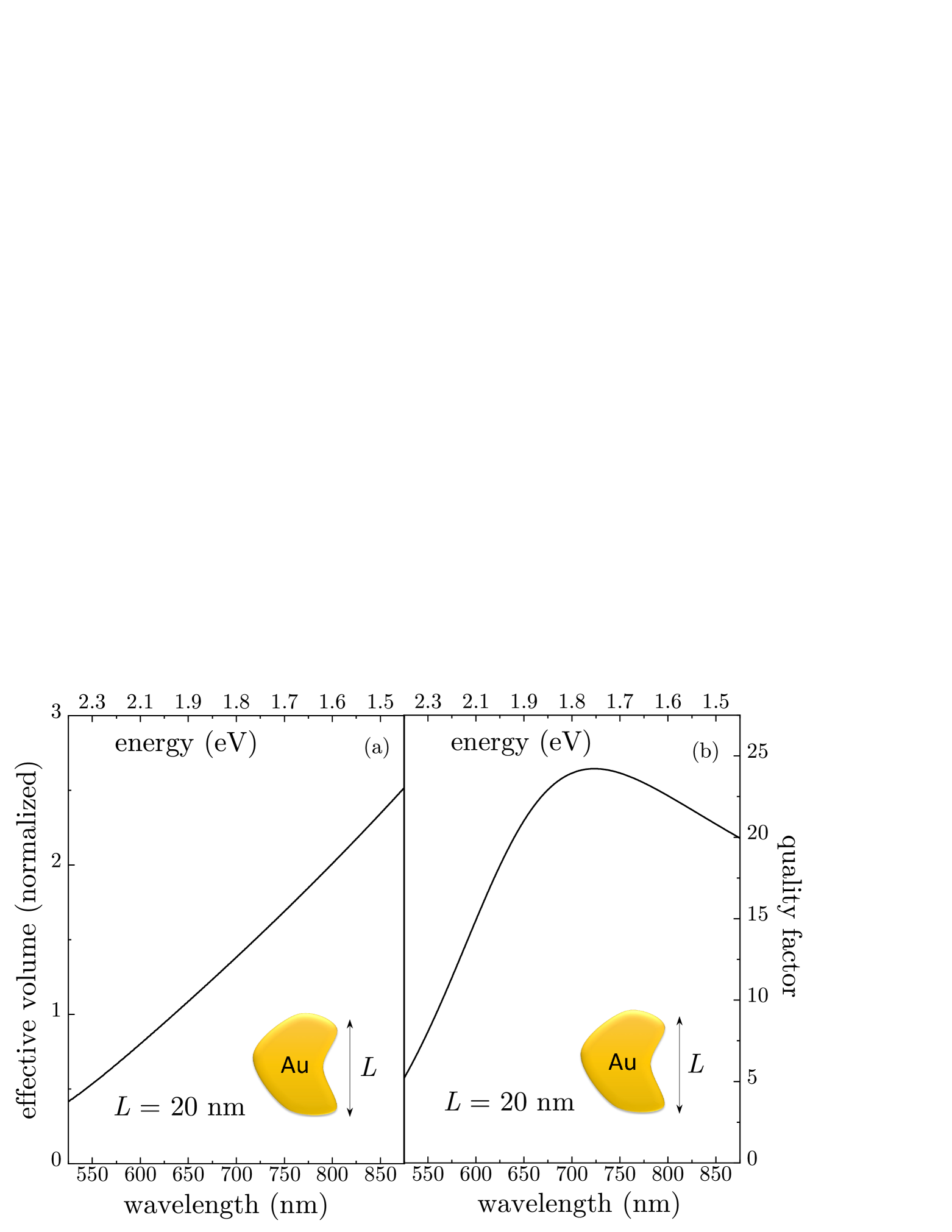
Figure 1: Normalized LSP effective volume $V_{n}/V_{m}$ (a) and quality factor $Q_{n}=\omega_{n}/\gamma_{n}$ (b) for an Au NP in water are plotted against the LSP wavelength. Inset: Schematics of Au NP of irregular shape with characteristic size $L=20$ nm.

The effect of temporal dispersion of metal dielectric function on the optical polarizability is illustrated in Figs. 1 and 2 for an Au NP placed in water ($\varepsilon_{d}=1.77$). We consider a NP with characteristic size $L=20$ nm and the metal volume $V_{\rm m}=L^{3}$, and use the experimental Au dielectric function in all calculations. For simplicity, we assume that incident light polarization is aligned with that of LSP and set $s_{n}=1$ hereafter. In Fig. (1), we plot the normalized effective volume $V_{n}/V_{\rm m}$ and the LSP quality factor $Q_{n}=\omega_{n}/\gamma_{n}$ versus the LSP wavelength. The effective volume, which is determined by $\varepsilon^{\prime}(\omega_{n})$, increases monotonically with the LSP wavelength, while the quality factor first increases but exhibits a maximum at about 700 nm due to non-monotonic behavior of $\varepsilon^{\prime\prime}(\omega_{n})$.

The frequency dependence of system parameters determines the amplitude and width of LSP-dominated extinction and scattering spectra shown in Fig. (2). The spectra we calculated for LSP wavelengths $\lambda_{n}=610$ nm, 670 nm, and 730 nm using non-Lorentzian polarizability (16) and its Lorentzian approximation (17). In fact, the Lorentzian approximation is largely accurate except a noticeable blueshift in the shorter wavelength region. Later in this paper we demonstrate that, in the presence of QEs resonantly coupled to the LSP, non-Lorentzian effects lead to dramatic changes in the optical spectra as the system tranzitions to strong coupling regime.

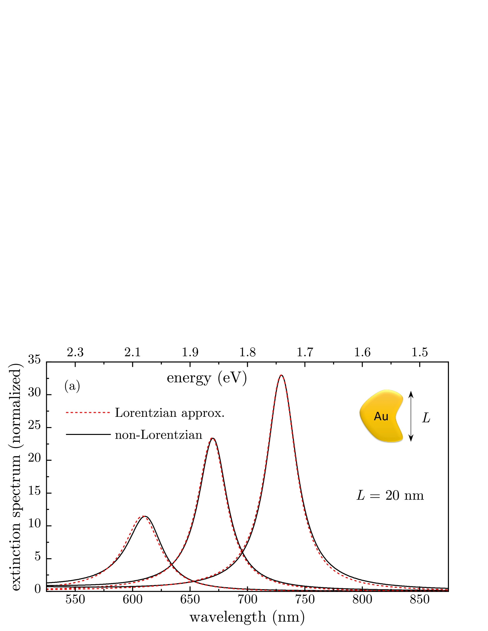
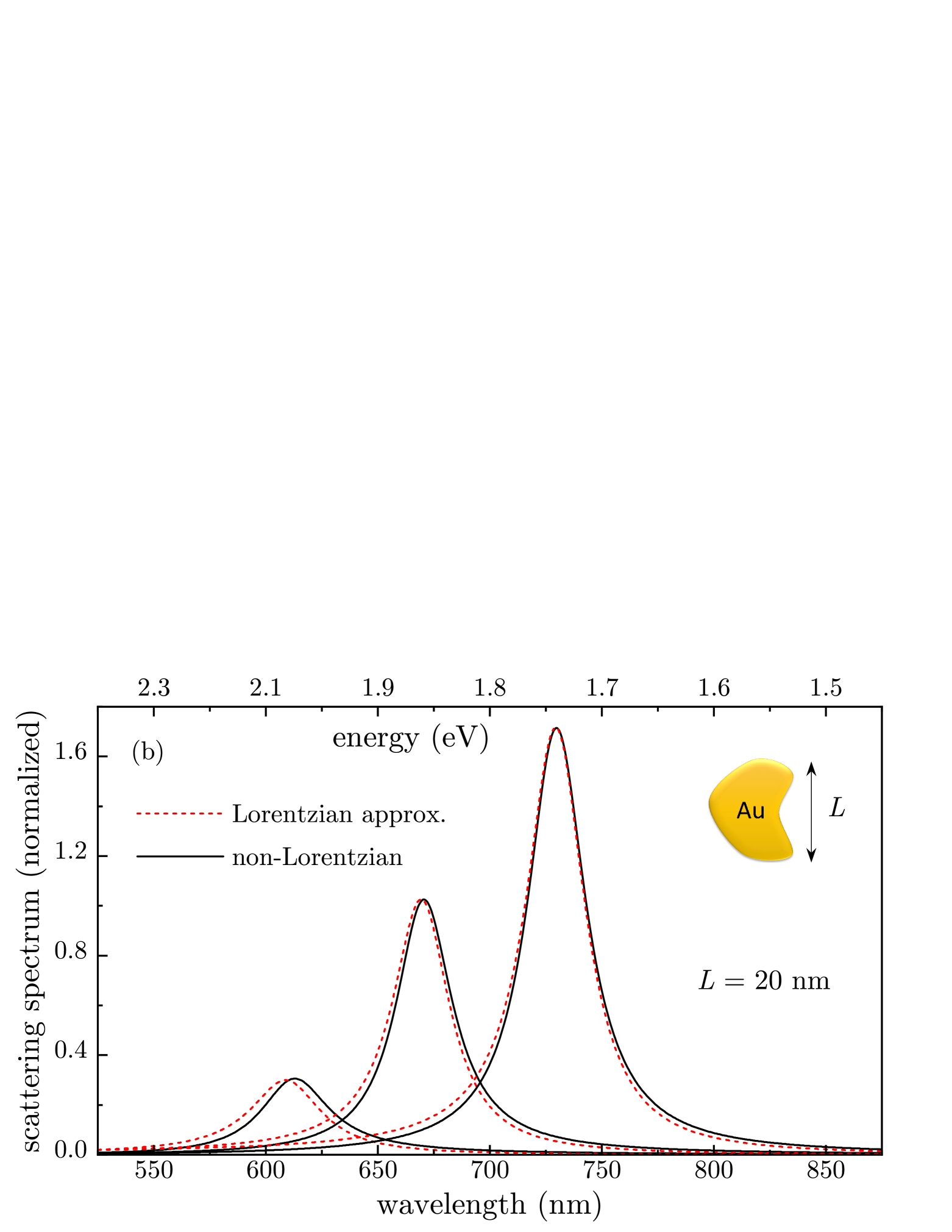
Figure 2: Normalized extinction cross-section $\sigma_{\rm ext}/L^{2}$ (a) and scattering cross-section $\sigma_{\rm scatt}/L^{2}$ (b) for an Au NP in water at LSP wavelengths 610 nm, 670 nm, and 730 nm calculated using non-Lorentzian and Lorentzian models.

III non-Lorentzian model for quantum emitters interacting with localized surface plasmons

In this section, we establish non-Lorentzian Maxwell-Bloch (MB) equations describing optical interactions of $N$ QEs with a resonant LSP mode. Each QE is characterized by optical polarizability

$$\bm{\alpha}_{i}(\omega)=\frac{1}{\hbar}\frac{\bm{\mu}_{i}\bm{\mu}_{i}}{\omega_{i}-\omega-\frac{i}{2}\gamma_{i}},$$ (19)

where $\omega_{i}$ is QE’s excitation frequency close to resonance with the LSP frequency $\omega_{n}$, $\gamma_{i}$ is the linewidth, and $\bm{\mu}_{i}=\mu_{i}\bm{n}_{i}$ is the dipole moment ($\bm{n}_{i}$ is its orientation). In the presence of incident light $\bm{E}_{0}e^{-i\omega t}$, the induced dipole moment of LSP mode has the form [compare to Eq. (12)]

$$\bm{p}_{n}=\dfrac{\varepsilon^{\prime}_{n}}{\hbar}\frac{\bm{\mu}_{n}(\omega)\,\bm{\mu}_{n}\!\cdot\!\bm{E}_{0}}{\varepsilon^{\prime}(\omega_{n})-\varepsilon(\omega)}+\bm{p}_{ne},$$ (20)

where $\bm{p}_{ne}=\int dV_{\rm m}\chi(\omega)\bm{E}_{e}$ is LSP dipole induced by the QEs’ electric field

$$\bm{E}_{e}(\bm{r})=\sum_{i}\bm{D}_{n}(\omega;\bm{r},\bm{r}_{i})\bm{p}_{i}=\sum_{i}\dfrac{\varepsilon^{\prime}_{n}}{\hbar}\frac{\tilde{\bm{E}}_{n}(\bm{r})\tilde{\bm{E}}_{n}(\bm{r}_{i})\!\cdot\!\bm{p}_{i}}{\varepsilon^{\prime}(\omega_{n})-\varepsilon(\omega)}.$$ (21)

Here, $\bm{p}_{i}$ are the induced dipole moments of QEs and $\bm{D}_{n}(\omega;\bm{r},\bm{r}_{i})$ is the LSP mode Green function (9). In terms of QE’s induced polarizations $\rho_{i}$, defined as $\bm{p}_{i}=\bm{\mu}_{i}\rho_{i}$, the QE-induced LSP dipole moment takes the form

$$\bm{p}_{ne}=\frac{\varepsilon^{\prime}_{n}\bm{\mu}_{n}(\omega)}{\varepsilon^{\prime}(\omega_{n})-\varepsilon(\omega)}\sum_{i}g_{in}\rho_{i}$$ (22)

where $g_{in}=\bm{\mu}_{i}\cdot\tilde{\bm{E}}_{n}(\bm{r}_{i})/\hbar$ is the QE-LSP coupling. Then the induced LSP dipole moment (20) takes the form

$$\bm{p}_{n}=\frac{\varepsilon^{\prime}_{n}\bm{\mu}_{n}(\omega)}{\varepsilon^{\prime}(\omega_{n})-\varepsilon(\omega)}\left(\sum_{i}g_{in}\rho_{i}+\bm{\mu}_{n}\!\cdot\!\bm{E}_{0}/\hbar\right),$$ (23)

Finally, defining LSP polarization $\rho_{n}$ through the relation $\bm{p}_{n}=\bm{\mu}_{n}(\omega)\rho_{n}$, we obtain the first MB equation as

$$\Omega_{n}\rho_{n}=\sum_{i}g_{in}\rho_{i}+\bm{\mu}_{n}\!\cdot\!\bm{E}_{0}/\hbar,$$ (24)

where $\Omega_{n}(\omega)=[\varepsilon^{\prime}(\omega_{n})-\varepsilon(\omega)]/\varepsilon^{\prime}_{n}$. In the Lorentzian limit, by expanding $\varepsilon(\omega)$ near $\omega_{n}$ we obtain $\Omega_{n}^{L}=\omega_{n}-\omega-i\gamma_{n}/2$, recovering the MB equation for LSP polarization $\rho_{n}$ [48]. The second MB equation for QEs’ polarization has the standard form

$$\Omega_{i}\rho_{i}=g_{in}\rho_{n}+\bm{\mu}_{i}\!\cdot\!\bm{E}_{0}/\hbar,$$ (25)

where $\Omega_{i}(\omega)=\omega_{i}-\omega-\frac{i}{2}\gamma_{i}$.

The coupled system of Eqs.  (24) and (25) represents non-Lorentzian extension of coupled MB equations for polarizations $\rho_{n}$ and $\rho_{i}$ as $\Omega_{n}(\omega)$ now incorporates the complex metal dielectric function $\varepsilon(\omega)$. Importantly, the LSP dipole moment $\bm{p}_{n}(\omega)=\bm{\mu}_{n}(\omega)\rho_{n}$ has additional dependence on $\varepsilon(\omega)$ via $\bm{\mu}_{n}(\omega)=[\varepsilon(\omega)-1]\int dV_{\rm m}\tilde{\bm{E}}_{n}(\bm{r})/4\pi$. Note that the QE-LSP coupling parameter $g_{in}$ is frequency independent and, using Eq. (8), can be recast in a cavity-like form as [7]

$$g^{2}_{in}=\frac{2\pi\mu_{i}^{2}\omega_{n}}{\hbar{\cal V}^{(i)}_{n}},~~\frac{1}{{\cal V}^{(i)}_{n}}=\frac{2[\bm{n}_{i}\!\cdot\!\bm{E}_{n}(\bm{r}_{i})]^{2}}{\int\!dV[\partial(\omega_{n}\varepsilon^{\prime})/\partial\omega_{n}]\bm{E}_{n}^{2}},$$ (26)

where ${\cal V}^{(i)}_{n}$ is projected LSP mode volume that characterizes the LSP field confinement at a point $\bm{r}_{i}$ in the direction $\bm{n}_{i}$ [55, 57, 56].

In the linear regime, the non-Lorentzian MB equations can be straightforwardly solved. First, it follows from Eq. (25) that

$$\sum_{i}g_{in}\rho_{i}=\Sigma_{n}\rho_{n}+\bm{q}_{n}\!\cdot\!\bm{E}_{0}/\hbar,$$ (27)

where $\bm{q}_{n}=\sum_{i}\bm{q}_{in}$ and $\bm{q}_{in}=\bm{\alpha}_{i}(\omega)\tilde{\bm{E}}_{n}(\bm{r}_{i})$ is QE’s dipole moment induced by the LSP mode field, while

$$\Sigma_{n}(\omega)=\frac{1}{\hbar}\sum_{i}\bm{q}_{n}\!\cdot\!\tilde{\bm{E}}_{n}(\bm{r}_{i})=\sum_{i}\frac{g_{in}^{2}}{\Omega_{i}(\omega)},$$ (28)

is LSP’s self-energy due to its coupling to QEs. Using Eq. (27) in Eq. (24), the LSP induced dipole moment is obtained as

$$\bm{p}_{n}(\omega)=\frac{\bm{\mu}_{n}(\omega)}{\hbar}\frac{[\bm{\mu}_{n}+\bm{q}_{n}(\omega)]\!\cdot\!\bm{E}_{0}}{\Omega_{n}(\omega)-\Sigma_{n}(\omega)}.$$ (29)

In a similar manner, the QE’ combined dipole moment $\bm{p}_{e}=\sum_{i}\bm{p}_{i}$ is obtained as

$$\bm{p}_{e}(\omega)=\frac{\bm{q}_{n}(\omega)}{\hbar}\frac{[\bm{\mu}_{n}+\bm{q}_{n}(\omega)]\!\cdot\!\bm{E}_{0}}{\Omega_{n}(\omega)-\Sigma_{n}(\omega)}+\bm{\alpha}_{N}(\omega)\bm{E}_{0}.$$ (30)

where $\bm{\alpha}_{N}(\omega)=\sum_{i}\bm{\alpha}_{i}(\omega)$. The combination $\bm{\mu}_{n}+\bm{q}_{n}$ in the numerator of Eqs. (29) and (30) indicates that the LSP optical dipole is now enhanced by LSP-mode-induced dipole of QEs excited in-phase by the LSP near field. The system full dipole moment is $\bm{p}(\omega)=\bm{p}_{n}(\omega)+\bm{p}_{e}(\omega)$ that defines the system’s effective optical polarizability, as discussed in the following section.

IV Effective polarizability and optical spectra

Here we obtain the effective polarizability for a single QE strongly coupled to the LSP. For a single QE, we have $\bm{q}_{n}=\bm{q}_{in}=g\bm{\mu}_{i}/\Omega_{i}(\omega)$ and $\Sigma_{n}(\omega)=g^{2}/\Omega_{i}(\omega)$, where we denoted the coupling as $g\equiv g_{in}=\bm{\mu}_{i}\!\cdot\!\tilde{\bm{E}}_{n}(\bm{r}_{i})/\hbar$. The induced dipole moments (29) and (30) take, respectively, the form

$$\bm{p}_{n}(\omega)=\frac{\bm{\mu}_{n}(\omega)}{\hbar}\frac{[\bm{\mu}_{n}+g\bm{\mu}_{i}/\Omega_{i}(\omega)]\!\cdot\!\bm{E}_{0}}{\Omega_{n}(\omega)-g^{2}/\Omega_{i}(\omega)}$$ (31)

and

$$\bm{p}_{i}(\omega)=\frac{\bm{\mu}_{i}}{\hbar}\frac{[\bm{\mu}_{i}+g\bm{\mu}_{n}/\Omega_{n}(\omega)]\!\cdot\!\bm{E}_{0}}{\Omega_{i}(\omega)-g^{2}/\Omega_{n}(\omega)}.$$ (32)

In Eq. (31), the first term represents contribution of the plasmonic antenna coupled to the emitter, while the second term describes interference effect when the light is first absorbed by the LSP-mode-induced QE dipole moment $\bm{q}_{in}(\omega)$ and then re-emitted by the antenna. In Eq. (32), the first term represents contribution of the QE coupled to the plasmonic antenna, while the second term describes interference effect when the light is first absorbed by the antenna and then re-emitted by the LSP-mode-induced QE dipole moment $\bm{q}_{in}(\omega)$.

In the following, we assume, for simplicity, that LSP’s and QE’s dipole orientations are aligned with the incident field polarization, i.e., $\bm{E}_{0}\parallel\bm{\mu}_{n}\parallel\bm{\mu}_{i}$. In this case, we have $\bm{p}_{n}(\omega)=\tilde{\alpha}_{n}(\omega)\bm{E}_{0}$ and $\bm{p}_{i}(\omega)=\tilde{\alpha}_{i}(\omega)\bm{E}_{0}$ for induced moments (31) and (32), respectively, where $\tilde{\alpha}_{n}(\omega)$ and $\tilde{\alpha}_{i}(\omega)$ are the corresponding effective polarizabilities. The effective antenna polarizability $\tilde{\alpha}_{n}(\omega)$ has the form

$$\tilde{\alpha}_{n}(\omega)=\frac{1}{\hbar}\frac{\mu_{n}(\omega)\mu_{n}f_{n}(\omega)}{\Omega_{n}(\omega)-g^{2}/\Omega_{i}(\omega)}$$ (33)

where the function $f_{n}(\omega)=1+g\mu_{i}/\mu_{n}\Omega_{i}(\omega)$ describes Fano interference between the plasmonic antenna and LSP-mode-induced QE dipole in the scattering spectra. Since the LSP dipole moment is much larger than that of QE, $\mu_{n}/\mu_{i}\gg 1$, for a single QE the Fano interference effects are relatively weak ($f_{n}\approx 1$) although they can be significant for many QEs [48]. At the same time, the effective QE polarizability has the form

$$\tilde{\alpha}_{i}(\omega)=\frac{1}{\hbar}\frac{\mu_{i}^{2}f_{i}(\omega)}{\Omega_{i}(\omega)-g^{2}/\Omega_{n}(\omega)},$$ (34)

where the function $f_{i}(\omega)=1+g\mu_{n}/\mu_{i}\Omega_{n}(\omega)$ describes Fano interference between the LSP-mode-induced QE dipole and plasmonic antenna. Since $\mu_{n}/\mu_{i}\gg 1$, the interference contribution to $\tilde{\alpha}_{i}$ is dominant ($f_{i}\gg 1$), in contrast to $\tilde{\alpha}_{n}$. Note, however, that both interference contributions are of the same order of magnitude while being much smaller than that of plasmonic antenna.

The effective polarizability of the QE-LSP system is $\tilde{\alpha}(\omega)=\tilde{\alpha}_{n}(\omega)+\tilde{\alpha}_{i}(\omega)$, which defines the extinction and scattering cross-sections according to Eq. (18). Similar to NP polarizability (16), the radiative damping is included in QE-LSP system’s effective polarizability by replacement $\tilde{\alpha}\rightarrow\tilde{\alpha}\left[1-(2i/3)k^{3}\tilde{\alpha}\right]^{-1}$. The Lorenntzian approximation is obtained by replacing $\Omega_{n}(\omega)=[\varepsilon^{\prime}(\omega_{n})-\varepsilon(\omega)]/\varepsilon^{\prime}_{n}$ with $\Omega_{n}^{L}(\omega)=\omega_{n}-\omega-i\gamma_{n}/2$ and $\mu_{n}(\omega)$ with $\mu_{n}(\omega_{n})\equiv\mu_{n}$ in Eqs. (33) and (34).

For a single QE, the QE’s coupling to radiation is negligibly small as compared to LSP, so the main contribution to the system effective polarizability comes from the plasmonic antenna contribution Eq. (33) (with $f_{n}=1$), which can be recast as [compare to Eq. (16)]

$$\tilde{\alpha}_{n}(\omega)=\dfrac{V_{n}[\varepsilon(\omega)-\varepsilon_{d}]}{\varepsilon(\omega)-\varepsilon^{\prime}(\omega_{n})\!-\!\frac{2i}{3}k^{3}V_{n}[\varepsilon(\omega)\!-\!\varepsilon_{d}]-\frac{\varepsilon^{\prime}_{n}g^{2}}{\omega-\omega_{i}+i\gamma_{i}/2}}.$$ (35)

In the Lorentzian approximation, the above expression reduces to [compare to Eq. (17)]

$$\tilde{\alpha}_{n}^{L}(\omega)=\frac{\mu_{n}^{2}}{\hbar}\frac{\omega_{i}-\omega-i\gamma_{i}/2}{(\omega_{n}-\omega-i\gamma_{n}/2)(\omega_{i}-\omega-i\gamma_{i}/2)-g^{2}},$$ (36)

which coincides with the effective polarizability obtained within CO model [33]. In the following section, show that non-Lorentzian effects strongly affect the optical spectra as the system transitions to strong coupling regime.

V Discussion and numerical results

Here we illustrate the role of non-Lorentzian effects in the transition to strong coupling regime for a QE situated near an Au NP in water ($\varepsilon_{d}=1,77$) with excitation frequency in resonance with LSP frequencies, i.e., $\omega_{i}=\omega_{n}$, considered here as input parameters. The NP characteristic size $L$, which defines its volume as $V_{\rm m}=L^{3}$, is chosen $L=20$ nm, and the experimental Au dielectric function is used in all calculations. The QE dipole moment, LSP polarization and incident light polarization are all aligned. The ratio of QE and LSP dipole moments is taken $\mu_{i}/\mu_{n}=10^{-4}$ while the ratio of QE and LSP spectral widths is taken $\gamma_{i}/\gamma_{n}=0.2$. For a single QE, the largest by far contributions come from the antenna’s polarizability (35) and its Lorentzian counterpart (36) although all contributions are included in the numerical calculations below.

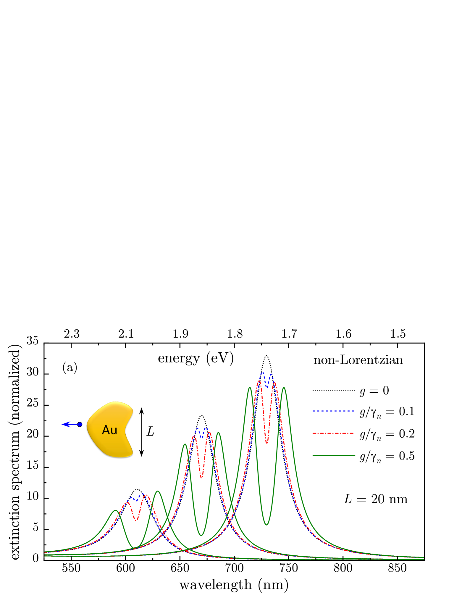
Figure 3: Normalized extinction cross-section $\sigma_{\rm ext}/L^{2}$ calculated using non-Lorentzian model (a) and its Lorentzian approximation (b) for a QE near Au NP in water at LSP wavelengths 610 nm, 670 nm, and 730 nm. Inset: Schematics of a QE near Au NP of irregular shape.

In Fig. (3) we show the normalized extinction spectra $\sigma_{\rm ext}/L^{2}$ calculated using our non-Lorentzian model [see Fig. (3(a)] and its Lorentzian approximation [see Fig. (3(b)] for LSP wavelengths 610 nm, 670 nm and 730 nm. With increasing ratio of QE-LSP coupling $g$ to LSP decay rate $\gamma_{n}$, the spectra first develop a narrow minimum corresponding to exciton-induced transparency (ExIT) [33, 34, 35, 58] which, with further increase of $g/\gamma_{n}$, transforms into the Rabi splitting signaling system’s transition to strong coupling regime. From the Lorentzian model (36), the frequencies of polaritonic states are $\omega_{\pm}=\omega_{n}-i(\gamma_{n}+\gamma_{i})/4\pm\sqrt{g^{2}-(\gamma_{n}-\gamma_{i})^{2}/16}$, implying that, for $\gamma_{i}/\gamma_{n}\ll 1$, strong coupling transition occurs at $g\gtrsim\gamma_{n}/4$. For smaller coupling, both polaritonic bands are centered at the same frequency $\omega_{n}$ while the ExIT minimum is caused by energy transfer from the LSP to QE within QE’s absorption spectral width $\gamma_{i}$ [58].

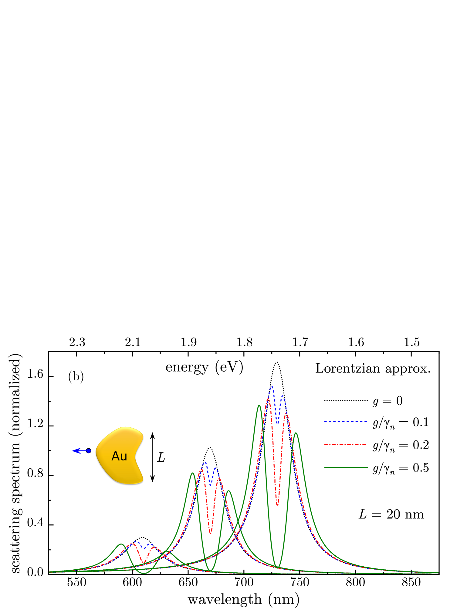
Figure 4: Normalized extinction cross-section $\sigma_{\rm ext}/L^{2}$ calculated using non-Lorentzian model (a) and its Lorentzian approximation (b) for a QE near Au NP in water at LSP wavelengths 610 nm, 670 nm, and 730 nm. Inset: Schematics of a QE near Au NP of irregular shape.

The striking difference between the spectra calculated using non-Lorentzian model and its Lorentzian approximation is the relative enhancement of lower energy polaritonic band clearly visible in Fig. 3(a) for wavelengths below 700 nm whereas the Lorentzian approximation, similar to CO model, leads to the enhancement of upper energy polaritonic band in the entire spectral range [see Fig. 3(b)]. This change of spectral asymmetry pattern persists at any value of coupling $g$ as the system transitions from the weak to strong coupling regime, indicating that this is a general non-Lorentzian effect independent of the coupling strength. This effect is even more visible in scattering spectra, shown in Fig. 4 for the same system parameters, which exhibit a prominent but opposite asymmetry pattern in the wavelengths region below 700 nm for normalized scattering cross-section $\sigma_{\rm scatt}/L^{2}$ calculated using non-lorentzian model in Fig. 4(a), and its Lorentzian approximation in Fig. 4(b). These results are consistent with the recent experiment on tip-enhanced strong-coupling spectroscopy of a single QE [31].

Qualitatively, the enhancement of lower energy polaritonic band originates from the presence of frequency-dependent metal dielectric function $\varepsilon(\omega)$ in the numerator of Eq. (35), whose real part behaves as $\varepsilon^{\prime}(\omega)\propto\omega^{-2}$, resulting in a suppression of the upper energy polarization band. At the same time, the asymmetry reversal for wavelengths above 700 nm seen in Figs. 3(a) and 4(a) can be traced to non-monotonic frequency dependence of the imaginary part of Au dielectric function $\varepsilon^{\prime\prime}(\omega)$, as revealed by the LSP quality factor shown in Fig. 1(b). Note that the Lorentzian polarizability (36) has no dependence on $\varepsilon(\omega)$ and so the spectral weight of polaritonic bands is determined solely by the powers of $\omega$ in the expressions (18) for extinction and scattering cross-sections which lead to enhancement of the upper energy polarization band in Figs. 3(b) and 4(b).

VI Conclusions

We have developed non-Lorentzian model for quantum emitters (QE) resonantly coupled to localized surface plasmons (LSP) in metal-dielectric structures. Using the exact LSP Green function, we derived non-Lorentzian version of Maxwell-Bloch equations which describe LSP in terms of metal complex dielectric function rather than of Lorentzian resonances. For a single QE coupled to the LSP, we obtained an explicit expression for the system effective optical polarizability which, in the Lorentzian approximation, recovers the classical coupled oscillator (CO) model. We demonstrated that non-Lorentzian effects originating from the temporal dispersion of metal dielectric function affect dramatically the optical spectra as the system transitions to the strong coupling regime. Specifically, in the plasmonic frequency region, the main spectral weight is shifted towards the lower energy polaritonic band, consistent with the experiment.

- [1] T. Schwartz, J. A. Hutchison, C. Genet, and T. W. Ebbesen, Phys. Rev. Lett. 106, 196405 (2011).
- [2] A.-L. Baudrion, A. Perron, A. Veltri, A. Bouhelier, P.-M. Adam, and R. Bachelot, Nano Lett. 13, 282–286 (2013).
- [3] L. Lin, M. Wang, X. Wei, X. Peng, C. Xie, and Y. Zheng, Nano Lett. 16, 7655–7663 (2016).
- [4] S. Sun, H. Kim, G. S. Solomon, and E. Waks, Nat. Nanotechnol. 11, 539–544 (2016).
- [5] L. De Santis, C. Anton, B. Reznychenko, N. Somaschi, G. Coppola, J. Senellart, C. Gomez, A. Lemaitre, I. Sagnes, A. G. White, L. Lanco, A. Auffeves, and P. Senellart, Nat. Nanotech 12, 663–667 (2017).
- [6] A. Tsargorodska, M. L. Cartron, C. Vasilev, G.Kodali, O. A. Mass, J. J. Baumberg, P. L. Dutton, C. N. Hunter, P. Törmä, and G. J. Leggett, Nano Lett. 16, 6850-6856 (2016).
- [7] T. V. Shahbazyan, Nano Lett. 19, 3273–3279 (2019).
- [8] C. Tserkezis, A. I. Fernandez-Dominguez, P. A. D. Goncalves, F. Todisco, J. D. Cox, K. Busch, N. Stenger, S. I. Bozhevolnyi, N. A. Mortensen, and C. Wolff, Rep. Prog. Phys. 83, 082401 (2020).
- [9] L. Novotny and B. Hecht, Principles of Nano-Optics (CUP, New York, 2012).
- [10] J. P. Reithmaier, G. Sek, A. Löffler, C. Hofmann, S. Kuhn, S. Reitzenstein, L. V. Keldysh, V. D. Kulakovskii, T. L. Reinecke, and A. Forchel, Nature 432, 197 (2004).
- [11] G. Khitrova, H. M. Gibbs, M. Kira, S. W. Koch, and A. Scherer, Nature Phys. 2, 81 (2006).
- [12] K. Hennessy, A. Badolato, M. Winger, D. Gerace, M. Atatüre, S. Gulde, S. Fält, E. L. Hu, and A. Imamoglu, Nature 445, 896 (2006).
- [13] J. Bellessa, C. Bonnand, J. C. Plenet, and J. Mugnier, Phys. Rev. Lett. 93, 036404 (2004).
- [14] Y. Sugawara, T. A. Kelf, J. J. Baumberg, M. E. Abdelsalam, and P. N. Bartlett, Phys. Rev. Lett. 97, 266808 (2006).
- [15] G. A. Wurtz, P. R. Evans, W. Hendren, R. Atkinson, W. Dickson, R. J. Pollard, A. V. Zayats, W. Harrison, and C. Bower, Nano Lett. 7, 1297 (2007).
- [16] N. T. Fofang, T.-H. Park, O. Neumann, N. A. Mirin, P. Nordlander, and N. J. Halas, Nano Lett. 8, 3481 (2008).
- [17] J. Bellessa, C. Symonds, K. Vynck, A. Lemaitre, A. Brioude, L. Beaur, J. C. Plenet, P. Viste, D. Felbacq, E. Cambril, and P. Valvin, Phys. Rev. B 80, 033303 (2009).
- [18] A. E. Schlather, N. Large, A. S. Urban, P. Nordlander, and N. J. Halas, Nano Lett. 13, 3281 (2013).
- [19] W. Wang, P. Vasa, R. Pomraenke, R. Vogelgesang, A. De Sio, E. Sommer, M. Maiuri, C. Manzoni, G. Cerullo, and C. Lienau, ACS Nano 8, 1056 (2014).
- [20] G. Zengin, M. Wersäll, S. Nilsson, T. J. Antosiewicz, M. Käll, T. Shegai, Phys. Rev. Lett. 114, 157401 (2015).
- [21] T. K. Hakala, J. J. Toppari, A. Kuzyk, M. Pettersson, H. Tikkanen, H. Kunttu, and P. Torma, Phys. Rev. Lett. 103, 053602 (2009).
- [22] A. Berrier, R. Cools, C. Arnold, P. Offermans, M. Crego-Calama, S. H. Brongersma, and J. Gomez-Rivas, ACS Nano 5, 6226 (2011).
- [23] A. Salomon, R. J. Gordon, Y. Prior, T. Seideman, and M. Sukharev, Phys. Rev. Lett. 109, 073002 (2012).
- [24] A. De Luca, R. Dhama, A. R. Rashed, C. Coutant, S. Ravaine, P. Barois, M. Infusino, and G. Strangi, Appl. Phys. Lett. 104, 103103 (2014).
- [25] V. N. Peters, T. U. Tumkur, Jing Ma, N. A. Kotov, and M. A. Noginov, Opt. Express 24, 25653 (2016).
- [26] P. Vasa, R. Pomraenke, S. Schwieger, Y. I. Mazur, V. Kunets, P. Srinivasan, E. Johnson, J. E. Kihm, D. S. Kim, E. Runge, G. Salamo, and C. Lienau, Phys. Rev. Lett. 101, 116801 (2008).
- [27] D. E. Gomez, K. C. Vernon, P. Mulvaney, and T. J. Davis, Nano Lett. 10, 274 (2010).
- [28] D. E. Gomez, S. S. Lo, T. J. Davis, and G. V. Hartland, J. Phys. Chem. B 117, 4340 (2013).
- [29] A. Manjavacas, F. J. Garcia de Abajo, and P. Nordlander, Nano Lett. 11, 2318 (2011).
- [30] H. Gross, J. M. Hamm, T. Tufarelli, O. Hess, and B. Hecht, Sci. Adv. 4, eaar4906 (2018).
- [31] K.-D. Park, M. A. May, H. Leng, J. Wang, J. A. Kropp, T. Gougousi, M. Pelton, and M. B. Raschke, Sci. Adv. 5, eaav5931 (2019).
- [32] J. J. Baumberg, J. Aizpurua, M. H. Mikkelsen, and D. R. Smith, Nat. Mater. 18, 668–678 (2019).
- [33] X. Wu, S. K. Gray, and M. Pelton, Optics Express 18, 23633-23645 (2010).
- [34] H. Leng, B. Szychowski, M.-C. Daniel, and M. Pelton, Nat. Commun. 9, 4012 (2018).
- [35] M. Pelton, S. D. Storm, and H. Leng, Nanoscale 11, 14540-14552 ( 2019).
- [36] N. Christogiannis, N. Somaschi, P. Michetti, D. M. Coles, P. G. Savvidis, P. G. Lagoudakis, and D. G. Lidzey, Adv. Opt. Mater. 1, 503 (2013).
- [37] J. George, S. Wang, T. Chervy, A. Canaguier-Durand, G. Schaeffer, J.-M. Lehn, J. A. Hutchison, C. Genet, and T. W. Ebbesen, Faraday Discuss. 178, 281–294 (2015).
- [38] A. Shalabney, J. George, J. Hutchison, G. Pupillo, C. Genet and T. W. Ebbesen, Nature Comm. 6, 5981 (2015).
- [39] M. Wersäll, J. Cuadra, T. J. Antosiewicz, S. Balci, and T. Shegai, Nano Lett. 17, 551-558 (2017).
- [40] M. Wersäll, B. Munkhbat, D. G. Baranov, F. Herrera, J. Cao, T. J. Antosiewicz, and T. Shegai, ACS Photonics 6, 2570–2576 (2019).
- [41] D. Zheng, S. Zhang, Q. Deng, M. Kang, P. Nordlander, H. Xu, Nano Lett. 17, 3809 (2017).
- [42] J. Wen, H. Wang, W. Wang, Z. Deng, C. Zhuang, Y. Zhang, F. Liu, J. She, J. Chen , H. Chen, S. Deng, and N. Xu, Nano Lett. 17, 4689 (2017).
- [43] J. del Pino, J. Feist, and F. J. Garcia-Vidal, New J. Phys. 17, 053040 (2015).
- [44] T. Newman and J. Aizpurua, Optica 5, 1247 (2018).
- [45] S.-J. Ding, X. Li, F. Nan, Y.-T. Zhong, L. Zhou, X. Xiao, Q.-Q. Wang, and Z. Zhang Phys. Rev. Lett. 119, 177401 (2017).
- [46] T. V. Shahbazyan, Nanophotonics 10, 3735 (2021).
- [47] F. Shen, Z. Chen, L. Tao, B. Sun, X. Xu, J. Zheng, and J. Xu, ACS Photon. 8, 212 (2021).
- [48] Z. Scott, S. Muhammad, and T. V. Shahbazyan, J. Chem. Phys. 156, 194702 (2022).
- [49] T. V. Shahbazyan, Phys. Rev. B 105, 245411 (2022).
- [50] H. T. Dung, L. Knöll, and D.-G. Welsch, Phys. Rev. A 57, 3931 (1998).
- [51] T. G. Philbin, New J. Phys. 12 123008 (2010).
- [52] T. V. Shahbazyan, Phys. Rev. B 103, 045421 (2021).
- [53] T. V. Shahbazyan, Phys. Rev. A 107, L061503 (2023).
- [54] M. I. Stockman, in Plasmonics: Theory and Applications, edited by T. V. Shahbazyan and M. I. Stockman (Springer, New York, 2013).
- [55] T. V. Shahbazyan, Phys. Rev. Lett. 117, 207401 (2016).
- [56] T. V. Shahbazyan, Phys. Rev. B 98, 115401 (2018).
- [57] T. V. Shahbazyan, ACS Photon. 4, 1003 (2017).
- [58] T. V. Shahbazyan, Phys. Rev. B 102, 205409 (2020).