A note on the existence of self-similar profiles of the hydrodynamic formulation of the focusing nonlinear Schrödinger equation

Abstract

After performing the Madelung transformation, the nonlinear Schrödinger equation is transformed into a hydrodynamic equation akin to the compressible Euler equations with a certain dissipation. In this short note, we construct self-similar solutions of such system in the focusing case for any mass supercritical exponent. To the best of our knowledge these solutions are new, and may formally arise as potential blow-up profiles of the focusing NLS equation.

1 Introduction

1.1 Historical Background

Consider a complex-valued function $v(x,t)$ solving the nonlinear Schrödinger equation (NLS):

$$i\partial_{t}v(x,t)+\Delta v(x,t)+\mu(v|v|^{p-1})(x,t)=0,$$ (1.1)

where $p$ is an odd integer and $\mu\in\{-1,1\}$. Other than the $L^{2}$ norm of $v$, the Hamiltonian given by

$$E(v)=\frac{1}{2}\int_{\mathbb{R}^{d}}|\nabla v|^{2}-\mu\frac{1}{p+1}\int_{\mathbb{R}^{d}}|v|^{p+1}$$

is also conserved. Note that if $\mu=-1$ the equation is called defocusing while if $\mu=1$ the equation is focusing.

The NLS (1.1) has a natural scaling, namely if $v$ is a solution and we set $v_{\lambda}(x,t)=\lambda^{2/(p-1)}v(\lambda x,\lambda^{2}t)$ then $v_{\lambda}$ is also a solution. The critical exponent $s_{c}$ for which the $\dot{H}^{s_{c}}$ norm remains invariant under scaling is given by $s_{c}=\frac{d}{2}-\frac{2}{p-1}$.

In the defocusing case ($\mu=-1$) it was expected that with enough regularity of the initial data one would always obtain global in time solutions. But in [18] Merle–Raphaël–Rodnianski–Szeftel proved finite time blow up for certain defocusing energy supercritical NLS, i. e. when $s_{c}>1$. In their proof the blow up solution was obtained by using as building blocks smooth, radial self-similar imploding solutions to a compressible Euler equation they had constructed in [19], (see also [2] by Buckmaster and the first two authors). In [5] the authors of this note generalized the space of functions for which there is blow-up for an energy supercritical focusing NLS equation to include also non radial initial data.

In the defocusing case, the connection mentioned above between NLS and compressible Euler equations occurs via the Madelung transform. In fact, via this transformation from the equation

$$i\partial_{t}v(x,t)+\Delta v(x,t)-(v|v|^{p-1})(x,t)=0,$$ (1.2)

one obtains (modulo exponentially small terms in self-similar coordinates) a set of equations equivalent to the compressible Euler ones, namely, for certain values of $\gamma>0$:

$$\begin{split}\rho\partial_{t}u+\rho u\cdot\nabla u&=-\frac{1}{\gamma}\nabla(\rho^{\gamma})+\nu\Delta u\\ \partial_{t}\rho+\rm{div}(\rho u)&=0.\end{split}$$ (1.3)

Motivated by the successful work on defocusing NLS mentioned above following this connection between NLS and fluid equations, in this note we use a similar approach to investigate blow-up questions for the focusing NLS

$$i\partial_{t}v(x,t)+\Delta v(x,t)+(v|v|^{p-1})(x,t)=0.$$ (1.4)

The ultimate goal would be finding a highly unstable blow-up profile for the focusing NLS in mass super-critical regime $\frac{d}{2}-\frac{2}{p-1}>0$.

Blow-up questions for focusing NLS equations have played a fundamental role in the study of dispersive equations, in particular in the last two decades. Here we are not going to give a full survey of the many results that have been proved in terms of blow-up, but we are going to mention only those necessary to frame the result that we are presenting in this note. From a virial argument [11] one can show that blow up can occur when the energy $E$ in (1.1) with $\mu=1$ is negative. There are two types of blow up for NLS, Type I blow up, which is self-similar, and the Type II which is not.

For the energy supercritical ($s_{c}>1$) focusing NLS equation there are no proved self-similar blow up results, the problem remains completely open. For Type II blow up, in the energy supercritical case, we recall [17]. If we assume that the problem is mass supercritical but energy subcritical, namely $0<s_{c}<1$ the picture is more complete.

Type II blow-up solutions of (1.4) were constructed in the mass critical case $s_{c}=0$ by Merle–Raphaël and Perelman in [13, 14, 16, 15, 23]. In all these results, all the blow-up profiles constructed are connected to the solitary wave $u(t,x)=e^{iwt}Q_{w}(x)$, where $Q_{w}$ is the unique radial and non negative solution to the elliptic equation:

$$\Delta Q_{w}-wQ_{w}+Q_{w}^{p}=0.$$

In the mass supercritical and energy subcritical case, $0<s_{c}<1$, the construction of blow-up solutions was carried out through solutions that blow up on a ring or sphere; see, for example, [9], [21], [24], and [12]. The Type I blow up in the range $0<s_{c}<1$ was conjectured in [25], and [26] and numerically supported, see for example [3] and references within. This conjecture has been proved in the range $0<s_{c}\ll 1$ in [20] ($1\leq d\leq 5$) and [1] ($d\geq 1$), and via a computer assisted proof in the case $d=p=3$ in [8] and [7]. In view of the lack of a complete picture of blow up in this mass supercritical regime it becomes relevant to look for blow up profiles using different methods, such as in this case the connection with fluid equations.

1.2 Setup of the problem

We now present the equation in hydrodynamical variables. Let us perform the Madelung transform and write $v=\sqrt{\rho}e^{i\psi}$. From (1.4), we have that

$$i\frac{\partial_{t}\rho}{2\sqrt{\rho}}e^{i\psi}-\partial_{t}\psi\sqrt{\rho}e^{i\psi} =-\left(\sqrt{\rho}e^{i\psi}\right)\rho^{\frac{p-1}{2}}-\Delta(\sqrt{\rho})e^{i\psi}-\frac{\nabla\rho}{\sqrt{\rho}}i\nabla\psi e^{i\psi}-\sqrt{\rho}\mathrm{div\,}\left(i\nabla\psi e^{i\psi}\right)$$ (1.5)

$$=\sqrt{\rho}e^{i\psi}\left(-\rho^{\frac{p-1}{2}}-\frac{\Delta(\sqrt{\rho})}{\sqrt{\rho}}-\frac{\nabla\rho}{\rho}i\nabla\psi-i\Delta\psi+|\nabla\psi|^{2}\right).$$ (1.6)

Now

$$\Delta\sqrt{\rho}=\mathrm{div\,}\left(\frac{\nabla\rho}{2\sqrt{\rho}}\right)=\frac{\Delta\rho}{2\sqrt{\rho}}-\frac{1}{4}\frac{|\nabla\rho|^{2}}{\rho^{3/2}}.$$

Since both $\rho$ and $\psi$ are real, we can identify real and imaginary parts in (1.5) and obtain

$$\begin{split}\partial_{t}\psi&=\rho^{\frac{p-1}{2}}+\frac{1}{2\rho}\Delta\rho-\frac{1}{4}\frac{|\nabla\rho|^{2}}{\rho^{2}}-|\nabla\psi|^{2}\\ \partial_{t}\rho&=2\left(-\nabla\rho\cdot\nabla\psi-\rho\Delta\psi\right)\end{split}$$ (1.7)

In order to see the similarity with the compressible Euler equations, we define $u=\nabla\psi$ and observe that the system takes the form

$$\partial_{t}u =\frac{p-1}{p+1}\frac{\nabla\left(\rho^{\frac{p+1}{2}}\right)}{\rho}-2u\nabla u+\nabla\left(\frac{\Delta\rho}{2\rho}-\frac{1}{4}\frac{|\nabla\rho|^{2}}{\rho^{2}}\right)$$

$$\partial_{t}\rho =-2u\nabla\rho-2\rho\mathrm{div\,}(u)=-2\mathrm{div\,}(u\rho).$$

We rescale time via $\partial_{t^{\prime}}=2\partial_{t}$. We have

$$\partial_{t^{\prime}}u =\frac{p-1}{2(p+1)}\frac{\nabla\left(\rho^{\frac{p+1}{2}}\right)}{\rho}-u\nabla u+\nabla\left(\frac{\Delta\rho}{4\rho}-\frac{1}{8}\frac{|\nabla\rho|^{2}}{\rho^{2}}\right)$$

$$\partial_{t^{\prime}}\rho =-\mathrm{div\,}(u\rho)$$

which corresponds to the compressible Euler equations for $\gamma=\frac{p+1}{2}$ and forcing $\nabla\Delta\sqrt{\rho}$ – the quantum pressure. See the survey [6] by Carles–Danchin–Saut for several aspects of the hydrodynamic formulation of NLS via the Madelung transform.

1.2.1 Self-similar equations

We let $\alpha=\frac{\gamma-1}{2}=\frac{p-1}{4}$. Setting the self-similar ansatz

$$\psi=\frac{(T-t)^{\frac{2}{r}-1}}{r}\Psi\left(\frac{x}{(T-t)^{1/r}},-\frac{\log(T-t)}{r}\right),$$

$$\rho=\frac{(T-t)^{\frac{1}{\alpha r}-\frac{1}{\alpha}}}{r}P\left(\frac{x}{(T-t)^{1/r}},-\frac{\log(T-t)}{r}\right)$$

and the variables

$$s=-\frac{\log(T-t)}{r},\qquad\mbox{ and }\qquad y=\frac{x}{(T-t)^{1/r}}=xe^{s}$$

in (1.7), we obtain

$$-(2-r)\Psi+y\nabla\Psi+\partial_{s}\Psi =r^{-2\alpha+2}P^{2\alpha}-|\nabla\Psi|^{2}+(T-t)^{2-\frac{4}{r}}\left(\frac{\Delta P}{2P}-\frac{|\nabla P|^{2}}{4P^{2}}\right)$$

$$-\frac{1-r}{\alpha}P+y\nabla P+\partial_{s}P =-2\nabla P\cdot\nabla\Psi-2P\Delta\Psi.$$

Therefore, we obtain

$$\begin{split}\partial_{s}\Psi&=(2-r)\Psi-y\nabla\Psi-|\nabla\Psi|^{2}+r^{-2\alpha+2}P^{2\alpha}+e^{(4-2r)s}\left(\frac{\Delta P}{2P}-\frac{|\nabla P|^{2}}{4P^{2}}\right)\\ \partial_{s}P&=\frac{1-r}{\alpha}P-y\nabla P-2\nabla P\cdot\nabla\Psi-2P\Delta\Psi.\\ \end{split}$$ (1.8)

Defining $S=2\frac{r^{1-\alpha}}{\sqrt{\alpha}}P^{\alpha}$, we have

$$\begin{split}\partial_{s}\Psi&=-(r-2)\Psi-y\nabla\Psi-|\nabla\Psi|^{2}+\frac{\alpha}{4}S^{2}+e^{(4-2r)s}\frac{\Delta(S^{1/(2\alpha)})}{S^{1/(2\alpha)}}\\ \partial_{s}S&=-(r-1)S-y\nabla S-2\nabla S\cdot\nabla\Psi-2\alpha S\Delta\Psi.\end{split}$$ (1.9)

One can also write the equation in $U,S$ variables, where $U=2\nabla\Psi$, yielding

$$\begin{split}\partial_{s}U&=-(r-1)U-y\nabla U-U\cdot\nabla U+\alpha S\nabla S+2e^{(4-2r)s}\frac{\Delta(S^{1/(2\alpha)})}{S^{1/(2\alpha)}}\\ \partial_{s}S&=-(r-1)S-y\nabla S-\nabla S\cdot U-\alpha S\text{div}(U).\end{split}$$ (1.10)

We will now look for $U,S$ that are radially symmetric, in a way that we can write $U=U_{R}\widehat{r}$ where $\widehat{r}$ is the unitary vector in the radial coordinate, and such that both functions are independent of $s$. Neglecting the exponentially decaying term, after substituting in (1.10) we obtain the following equations:

$$\begin{split}0&=-(r-1)U_{R}-\zeta\partial_{\zeta}U_{R}-U_{R}\partial_{\zeta}U_{R}+\alpha S\partial_{\zeta}S\\ 0&=-(r-1)S-\zeta\partial_{\zeta}S-\partial_{\zeta}SU_{R}-\alpha S\partial_{\zeta}U_{R}-\alpha(d-1)\frac{SU}{\zeta}.\end{split}$$ (1.11)

Now we apply the following extra transformation: we define $U_{R}=\zeta\overline{U}$ and $S=\zeta\overline{S}$. We then obtain that

$$\begin{split}0&=-(r-1)\overline{U}-\zeta\partial_{\zeta}\overline{U}-\overline{U}-\zeta\overline{U}\partial_{\zeta}\overline{U}-\overline{U}^{2}+\alpha\overline{S}^{2}+\alpha\zeta\overline{S}\partial_{\zeta}\overline{S}\\ 0&=-(r-1)\overline{S}-\zeta\partial_{\zeta}\overline{S}-\overline{S}-\zeta\overline{U}\partial_{\zeta}\overline{S}-\overline{U}\overline{S}-\alpha\zeta\overline{S}\partial_{\zeta}\overline{U}-\alpha\overline{U}\overline{S}-\alpha(d-1)\overline{U}\overline{S}.\end{split}$$ (1.12)

Letting $\partial_{\xi}=\zeta\partial_{\zeta}$

$$\begin{split}\partial_{\xi}\overline{U}+\overline{U}\partial_{\xi}\overline{U}-\alpha\overline{S}\partial_{\xi}\overline{S}&=-r\overline{U}-\overline{U}^{2}+\alpha\overline{S}^{2}\\ \partial_{\xi}\overline{S}+\overline{U}\partial_{\xi}\overline{S}+\alpha\overline{S}\partial_{\xi}\overline{U}&=-r\overline{S}-\overline{U}\overline{S}-\alpha d\overline{U}\overline{S}.\end{split}$$ (1.13)

We can rewrite this system as

$$\begin{pmatrix}1+\overline{U}&-\alpha\overline{S}\\ \alpha\overline{S}&1+\overline{U}\\ \end{pmatrix}\cdot\begin{pmatrix}\partial_{\xi}\overline{U}\\ \partial_{\xi}\overline{S}\end{pmatrix}=\begin{pmatrix}-r\overline{U}-\overline{U}^{2}+\alpha\overline{S}^{2}\\ -r\overline{S}-\overline{U}\overline{S}-\alpha d\overline{U}\overline{S}\end{pmatrix}.$$ (1.14)

The fundamental difference with the defocusing case is that here the matrix is not real diagonalizable. One can however still invert the matrix, and using

$$\begin{pmatrix}1+\overline{U}&-\alpha\overline{S}\\ \alpha\overline{S}&1+\overline{U}\\ \end{pmatrix}^{-1}=\frac{1}{(1+\overline{U})^{2}+\alpha^{2}\overline{S}^{2}}\begin{pmatrix}1+\overline{U}&\alpha\overline{S}\\ -\alpha\overline{S}&1+\overline{U}\\ \end{pmatrix}$$

and (1.13) yields

$$\partial_{\xi}\overline{U}=\frac{N_{U}}{D},\qquad\mbox{ and }\qquad\partial_{\xi}\overline{S}=\frac{N_{S}}{D}$$ (1.15)

for

$$D =\left(1+\overline{U}\right)^{2}+\alpha^{2}\overline{S}^{2},$$

$$N_{U} =(1+\overline{U})\left(-r\overline{U}-\overline{U}^{2}+\alpha\overline{S}^{2}\right)+\alpha\overline{S}\left(-r\overline{S}-\overline{U}\overline{S}-\alpha d\overline{U}\overline{S}\right)$$

$$N_{S} =-\alpha\overline{S}\left(-r\overline{U}-\overline{U}^{2}+\alpha\overline{S}^{2}\right)+(1+\overline{U})\left(-r\overline{S}-\overline{U}\overline{S}-\alpha d\overline{U}\overline{S}\right).$$ (1.16)

Another fundamental difference with the defocusing case is that here $D\neq 0$.

1.3 Main result

We now state the main result of this paper:

Theorem 1.1.

Assume that $\alpha d>r-1$, $\alpha=\frac{p-1}{4}$, with $p$ an odd natural number. Then there exists a smooth solution $(U_{R}(\zeta),S(\zeta))$ to (1.11) with decay at infinity. Moreover, $U_{R}$ admits a $C^{\infty}$ odd extension and $S$ admits a $C^{\infty}$ even extension with respect to $\zeta$, so that the $\mathbb{R}^{d}$ radially symmetric vector and scalar fields generated by $U_{R}$ and $S$, respectively, are smooth. Under the scaling symmetry, we can take $S(0)=1$ and $U^{\prime}_{R}(0)=-\frac{r-1}{\alpha d}.$

The proof is postponed to the next section and done in terms of the autonomous system (1.15). It is structured in the following steps:

1. We first perform an expansion of the solution as a series around $\xi=-\infty$.

2. Then, we can bound the coefficients of such expansion to prove its convergence for $\xi<-\log(8)$. At such point standard existence techniques for ODE apply, and we can continue the solution.

3. In order to prove that the limit of the solution as $\xi\to\infty$ is $(0,0)$, we apply barrier arguments (with the barriers $U=-1$ and $U=0$, see Figure 1 with an illustration of the phase portrait) to show that the solution will never cross them and thus the only possibility for such limit is the point $(0,0)$.

Remark 1.2.

In order to justify that it is ok to neglect the term $e^{(4-2r)s}\frac{\Delta(S^{1/(2\alpha)})}{S^{1/(2\alpha)}}$, we need to assume that $r>2$. By choosing $r=2+\varepsilon$, in terms of $p$, we obtain $(p-1)d>4(1+\varepsilon)$, so that for any $p>1+4/d$ we can find such $r$. This corresponds to a mass supercritical NLS equation. Indeed as mentioned above one has that

$$s_{c}=\frac{d}{2}-\frac{2}{p-1},$$

where the choice of $p_{L^{2}}=1+4/d$ corresponds $s_{c}=0$. Hence our condition $p>p_{L^{2}}$ corresponds to $s_{c}>0$, the mass supercritical case.

Remark 1.3.

The point $(0,0)$ is a focus of our phase portrait (cf. Figure 1). The rate of decay of any solution approaching it will be dictated by its eigenvalues, concretely if the Jacobian of the focus has eigenvalues $\lambda_{1}\leq\lambda_{2}<0$, all solutions will approach at the slower rate $e^{\lambda_{2}\xi}$, while two exceptional solutions (forming one smooth curve) will approach at rate $e^{\lambda_{1}\xi}$. Such considerations happen to be irrelevant in our case, since for our phase portrait linearized around $(0,0)$, the Jacobian of the field has a double eigenvalue $\lambda_{1}=\lambda_{2}=-r$. Thus, any solution (and in particular, our solution), will be $O(e^{-r\xi})$ for large $\xi$. After undoing the change $U_{R}=e^{\xi}\overline{U}$ and $S=\overline{S}e^{\xi}$ the original self-similar solution still decays, in this case at a rate $\frac{1}{R^{(r-1)}}$. This is actually exactly the same rate as the solutions in the defocusing case [19].

Remark 1.4.

It is very natural to try to upgrade the radial solution of (1.15) into a solution of (1.4) using the techniques developed in [19, 2, 4]. However, the lack of energy estimates and the ill-posedness in Sobolev spaces for the (1.10) focusing case lead to the need to work in analytic spaces [22]. See [10, 27] for local existence results in analytic spaces. Another point of view is that with the negative pressure law, the compressible Euler equation is now an elliptic rather than a hyperbolic system [6, Remark 2.2].

Remark 1.5.

Under the hydrodynamical variables we have that $|v|=\sqrt{\rho}$ and $\nabla v=v\left(\frac{\nabla\rho}{2\rho}+i\nabla\psi\right)$. Therefore, the focusing energy can be reexpressed as

$$E(\rho,\psi)=\int_{\mathbb{R}^{d}}\rho\left(\frac{|\nabla\psi|^{2}}{2}+\frac{|\nabla\rho|^{2}}{8\rho^{2}}-\frac{\rho^{\frac{p-1}{2}}}{p+1}\right)$$

Taking $t=0$ in our profiles, the inner parenthesis reads

$$\frac{T^{2/r-2}|\nabla\Psi|^{2}}{2r^{2}}+\frac{T^{-2/r}|\nabla P|^{2}}{8P^{2}}-\frac{T^{2/r-2}P^{2\alpha}}{(p+1)r^{2\alpha}}=T^{2/r-2}\left(\frac{|U|^{2}}{8r^{2}}+T^{2-4/r}\frac{|\nabla S|^{2}}{8\alpha^{2}S^{2}}-\frac{\alpha S^{2}}{4(p+1)r^{2}}\right)$$

If we fix the profile to be very close to the solution at the singular time, and using that $r>2$, the sign of the energy agrees with the sign of

$$\int_{0}^{\infty}S^{1/\alpha}\left(\frac{U^{2}}{2}-\frac{\alpha S^{2}}{p+1}\right)R^{d-1}dR$$

Numerically, we have observed that this value is negative for $d=3,p=10/3,r=21/10$.

1.4 Acknowledgements

GCL and GS have been supported by NSF under grant DMS-2052651 and DMS-2306378, and by the Simons Foundation Collaboration Grant on Wave Turbulence. GCL, JGS and JS have been partially supported by the MICINN (Spain) research grant number PID2021–125021NA–I00. JGS has been partially supported by NSF under Grants DMS-2245017, DMS-2247537 and DMS-2434314, and by the AGAUR project 2021-SGR-0087 (Catalunya). JS has been partially supported by an AMS-Simons Travel Grant. JGS is also thankful for the hospitality of the MIT Department of Mathematics, where parts of this paper were done.

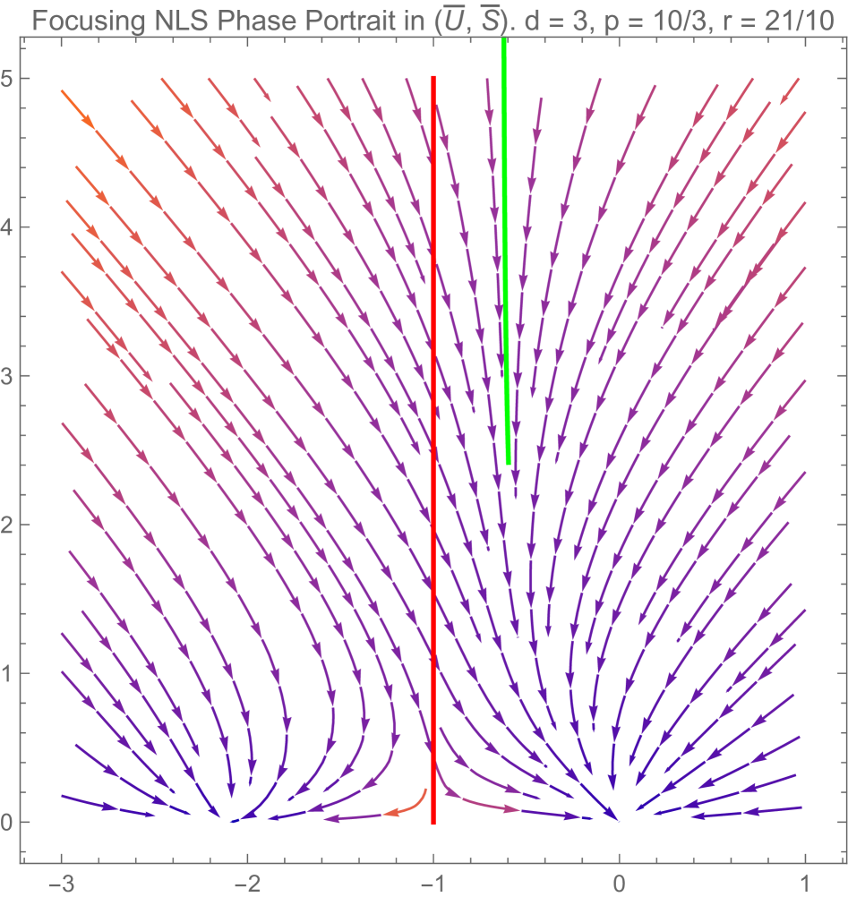
Figure 1: Green: Taylor series expansion starting from $P_{0}$. The trajectory will reach $(0,0)$. Red: barrier $\overline{U}=-1$. The solution needs to start from $(\overline{U},\overline{S})=(\overline{U}_{0},\infty)$ with $\overline{U}_{0}>-1$. There will exist values of $r>2$ such that this happens if and only if $(p,d)$ lie in the mass supercritical regime.

2 Proof of the Main Theorem

2.1 Expansion of the solution as a series

We consider the following expansion

$$\overline{U}=\sum_{\begin{subarray}{c}n=0\\ \text{ even }\end{subarray}}U_{n}e^{n\xi},\qquad\mbox{ and }\qquad\overline{S}=\sum_{\begin{subarray}{c}n=-1\\ \text{ odd }\end{subarray}}S_{n}e^{n\xi}.$$ (2.1)

Scaling symmetry allows us to fix $S_{-1}=1$. In order to deduce the recursion of the coefficients, it is convenient to consider the simplified expressions of $D,N_{u},N_{s}$ that one can obtain simplifying the above expressions (cf. (1.16)):

$$D =\left(1+\overline{U}\right)^{2}+\alpha^{2}\overline{S}^{2},$$

$$N_{U} =-\alpha^{2}d\overline{S}^{2}\overline{U}-\alpha(r-1)\overline{S}^{2}-\overline{U}(\overline{U}+1)(r+\overline{U})$$

$$N_{S} =-\alpha^{2}\overline{S}^{3}+\overline{S}\overline{U}(-\alpha d+\alpha r-r-1)+\overline{S}\overline{U}^{2}(\alpha(-d)+\alpha-1)-r\overline{S}.$$

Now, note that

$$D=\sum_{\begin{subarray}{c}n=-2\\ \text{even}\end{subarray}}D_{n}e^{n\xi},\qquad N_{U}=\sum_{\begin{subarray}{c}n=-2\\ \text{even}\end{subarray}}N_{U,n}e^{n\xi},\qquad N_{S}=\sum_{\begin{subarray}{c}n=-3\\ \text{odd}\end{subarray}}N_{S,n}e^{n\xi}.$$

The coefficients are given by

$$D_{n} =\delta_{n,0}+2U_{n}+\sum_{\begin{subarray}{c}i=0\\ \text{even}\end{subarray}}^{n}U_{i}U_{n-i}+\alpha^{2}\sum_{\begin{subarray}{c}i=-1\\ \text{odd}\end{subarray}}S_{i}S_{n-i}$$

$$N_{U,n} =-\alpha^{2}d\sum_{\begin{subarray}{c}i=-1\\ \text{odd }\end{subarray}}^{n+1}\sum_{\begin{subarray}{c}j=-1\\ \text{odd }\end{subarray}}^{n-i}S_{i}S_{j}U_{n-i-j}-\alpha(r-1)\sum_{\begin{subarray}{c}i=-1\\ \text{odd }\end{subarray}}^{n+1}S_{i}S_{n-i}-\sum_{\begin{subarray}{c}i=0\\ \text{even }\end{subarray}}^{n}\sum_{\begin{subarray}{c}j=0\\ \text{even }\end{subarray}}^{n-i}U_{i}U_{j}U_{n-i-j}-(r+1)\sum_{\begin{subarray}{c}i=0\\ \text{even }\end{subarray}}^{n}U_{i}U_{n-i}-rU_{n}$$

$$N_{S,n} =-\alpha^{2}\sum_{\begin{subarray}{c}i=-1\\ \text{odd }\end{subarray}}^{n+2}\sum_{\begin{subarray}{c}j=-1\\ \text{odd }\end{subarray}}^{n+1-i}S_{i}S_{j}S_{n-i-j}+(-\alpha d+\alpha r-r-1)\sum_{\begin{subarray}{c}i=-1\\ \text{odd }\end{subarray}}^{n}S_{i}U_{n-i}+(-\alpha d+\alpha-1)\sum_{\begin{subarray}{c}i=-1\\ \text{odd }\end{subarray}}^{n}\sum_{\begin{subarray}{c}j=0\\ \text{even }\end{subarray}}^{n-i}S_{j}U_{i}U_{n-i-j}-rS_{n}.$$

Moreover, we extract the top order terms of the numerators as follows

$$N_{U,n}=-\alpha^{2}dU_{n+2}+\widetilde{N}_{U,n},\qquad\mbox{ and }\qquad N_{S,n}=-3\alpha^{2}S_{n+2}+\widetilde{N}_{S,n}$$

where

$$\widetilde{N}_{U,n} =-\alpha^{2}d\sum_{\begin{subarray}{c}i=-1\\ \text{odd }\end{subarray}}^{n+1}\sum_{\begin{subarray}{c}j=(-1)\vee(-i)\\ \text{odd }\end{subarray}}^{n-i}S_{i}S_{j}U_{n-i-j}-\alpha(r-1)\sum_{\begin{subarray}{c}i=-1\\ \text{odd }\end{subarray}}^{n+1}S_{i}S_{n-i}-\sum_{\begin{subarray}{c}i=0\\ \text{even }\end{subarray}}^{n}\sum_{\begin{subarray}{c}j=0\\ \text{even }\end{subarray}}^{n-i}U_{i}U_{j}U_{n-i-j}-(r+1)\sum_{\begin{subarray}{c}i=0\\ \text{even }\end{subarray}}^{n}U_{i}U_{n-i}-rU_{n}$$

$$\widetilde{N}_{S,n} =-\alpha^{2}\sum_{\begin{subarray}{c}i=-1\\ \text{odd }\end{subarray}}^{n}\sum_{\begin{subarray}{c}j=(-1)\vee(-i)\\ \text{odd }\end{subarray}}^{(n+1-i)\wedge n}S_{i}S_{j}S_{n-i-j}+(-\alpha d+\alpha r-r-1)\sum_{\begin{subarray}{c}i=-1\\ \text{odd }\end{subarray}}^{n}S_{i}U_{n-i}+(-\alpha d+\alpha-1)\sum_{\begin{subarray}{c}i=-1\\ \text{odd }\end{subarray}}^{n}\sum_{\begin{subarray}{c}j=0\\ \text{even }\end{subarray}}^{n-i}S_{j}U_{i}U_{n-i-j}-rS_{n}.$$

We have removed the term $S_{-1}S_{-1}U_{n+2}=U_{n+2}$ on the first sum of $N_{U,n}$ and the term $S_{-1}S_{-1}S_{n+2}=S_{n+2}$ (and its permutations) on the first sum of $N_{S,n}$.

Now, we look at the series for $D\partial_{\xi}U$ and $D\partial_{\xi}S$. We have that

$$(D\partial_{\xi}U)_{n} =nU_{n}+2\sum_{\begin{subarray}{c}i=0\\ \text{even }\end{subarray}}^{n}iU_{i}U_{n-i}+\sum_{\begin{subarray}{c}i=0\\ \text{even }\end{subarray}}^{n}\sum_{\begin{subarray}{c}j=0\\ \text{even }\end{subarray}}^{n-i}iU_{i}U_{j}U_{n-i-j}+\alpha^{2}\sum_{\begin{subarray}{c}i=0\\ \text{even}\end{subarray}}^{n}iU_{i}\sum_{j=-1}^{n+1-i}S_{j}S_{n-i-j}+\alpha^{2}(n+2)U_{n+2}S_{-1}^{2}$$

$$(D\partial_{\xi}S)_{n} =nS_{n}+2\sum_{\begin{subarray}{c}i=-1\\ \text{odd }\end{subarray}}^{n}iS_{i}U_{n-i}+\sum_{\begin{subarray}{c}i=-1\\ \text{odd }\end{subarray}}^{n}\sum_{\begin{subarray}{c}j=0\\ \text{even }\end{subarray}}^{n-i}iS_{i}U_{j}U_{n-i-j}+\alpha^{2}\sum_{\begin{subarray}{c}i=-1\\ \text{odd}\end{subarray}}^{n}\sum_{j=(-1)\vee(-i)}^{(n+1-i)\wedge n}iS_{i}S_{j}S_{n-i-j}+\alpha^{2}nS_{n+2}S_{-1}^{2}.$$

Note again that we have isolated the main terms in the right. Defining $\widetilde{D}_{U,n}$ and $\widetilde{D}_{S,n}$ to be the rest and recalling $S_{-1}=1$, we obtain

$$(D\partial_{\xi}U)_{n}=\widetilde{D}_{U,n}+\alpha^{2}(n+2)U_{n+2},\qquad\mbox{ and }\qquad(D\partial_{\xi}S)_{n}=\widetilde{D}_{S,n}+\alpha^{2}nS_{n+2}.$$

Equaling each coefficient of $D\partial_{\xi}U$ with each coefficient of $N_{u}$ (and the same for $S$) the recurrence can be written as

$$\begin{cases}\left(\alpha^{2}(n+2)+\alpha^{2}d\right)U_{n+2}&=\widetilde{N}_{U,n}-\widetilde{D}_{U,n}\\ \left(\alpha^{2}n+3\alpha^{2}\right)S_{n+2}&=\widetilde{N}_{S,n}-\widetilde{D}_{S,n}\end{cases}$$ (2.2)

for every $n\geq-2$. Since $S_{-1}=1$, and the right hand sides depend at most on coefficients of order $(n+1)$, this allows to solve all the other coefficients as long as the parenthesis of the left hand side are positive since clearly $n+2+d>0$ and $n+3>0$.

2.2 Convergence of the series

Let us denote $p_{n}$ to be $1+|U_{n}|$ for even $n$ and $1+|S_{n}|$ for odd $n$. Let $n\geq 0$, it is clear that we have

$$\left|p_{n+2}\right|\leq C\sum_{i,j\geq-1}^{n+2}p_{i}p_{j}p_{n-i-j}\mathbbm{1}_{i,j,n-i-j\leq n+1}$$ (2.3)

for some absolute constant $C=C(\alpha,d)$. One can just directly observe this from the expressions of $\widetilde{N}_{U,n}$, $\widetilde{N}_{S,n}$, $\widetilde{D}_{U,n}$, $\widetilde{D}_{S,n}$, since no term with a coefficient $n+2$ appears there. In the cases where the expression is not trilinear, but just bilinear or linear it can be trivially bounded by the trilinear expression above taking $i=0$ (bilinear) or $i=j=0$ (linear) and noting $p_{0}\geq 1$ by definition. Moreover, in the case of $D_{U,n}$, $D_{S,n}$ some factors of $i$ appear, but those are smaller than the factor of $n$ that goes dividing from the companion factor of $U_{n+2}$ or $S_{n+2}$.

Now, we define $\overline{p}_{n}=\max_{i\leq n}p_{n}$. We take (2.3) and observe that it cannot happen that two of the three subindex are $-1$ (since then the other would be $n+2$). Therefore, there is at most one of them that is $-1$, and in that case we bound $p_{-1}\leq\overline{p}_{0}$. If no subindex is $-1$ we have $i\leq n$ and simply bound $p_{i}\leq\overline{p}_{i+1}$. We obtain

$$\left|\overline{p}_{n+2}\right|\leq 3C\sum_{\begin{subarray}{c}i,j,k\geq 0\\ i+j+k=n+1\end{subarray}}\overline{p}_{i}\overline{p}_{j}\overline{p}_{k}$$

where the factor of $3$ is because one triplet can come from at most three of the previous triplets (one of the three indices is a unit less in the previous sum).

Therefore, we see that $\overline{p}_{n}$ is bounded by the tri-Catalan numbers (also known as number of ternary trees). That is, the sequence defined by $\mathfrak{C}_{0}=1$ and

$$\mathfrak{C}_{n+1}=\sum_{\begin{subarray}{c}i,j,k\geq 0\\ i+j+k=n\end{subarray}}\mathfrak{C}_{i}\mathfrak{C}_{j}\mathfrak{C}_{k}.$$

They are known to obey an exponential bound $\mathfrak{C}_{n}\lesssim 8^{n}$. This shows the Taylor series is convergent for $e^{\xi}<1/8$, After that, we can just use standard ODE existence of solutions to continue our solution $\overline{U},\overline{S}$.

2.3 Existence of self-similar solutions

From the convergence of the Taylor series of the previous subsection, we can guarantee that a smooth solution self-similar solution exists for $\xi\in(-\infty,-\log(8))$ (corresponding to a radial solution on a ball of radius $1/8$ around the origin). Moreover, after undoing the change of variables $U_{R}=\zeta\overline{U}=e^{\xi}\overline{U}$, and $S=\zeta\overline{S}=e^{\xi}\overline{S}$, we obtain that the self-similar solution in $(U,S)$ coordinates is bounded, and that $U$ is odd, while $S$ is even.

Now, let us bound the global behaviour of the solution. We consider the barrier $\overline{U}=-1$. The sign of the normal component of the field $(N_{u}/D,N_{s}/D)$ to the barrier is just the sign of $N_{u}$ (given that the normal vector is $(1,0)$ and $D>0$). We have that

$$N_{U}(-1,S)=\alpha(1+\alpha d-r)S^{2}.$$

Therefore, when $\alpha d>r-1$ we have that this sign is positive and therefore solutions cannot traverse $U=-1$ from right to left.

Similarly, the formula for $\overline{U}_{0}$ can be computed from the Taylor recurrence and yields

$$\overline{U}_{0}=-1+\frac{\alpha d-(r-1)}{\alpha d}$$

so that $\overline{U}_{0}>-1$ also when $\alpha d>r-1$

Therefore, we conclude that the condition $\alpha d>r-1$ ensures that the solution starts in the region $\overline{U}>-1$ and moreover cannot exit that region. This condition is particularly interesting since it avoids the possibility of the solution reaching the attractor $(-r,0)$. On the other hand, this is a if and only if condition, since $\alpha d<r-1$ would imply that the solution starts at $\overline{U}<-1$ and remains there for all times (making it impossible for the solution to reach $(0,0)$). In the case $\alpha d=r-1$ one gets the trivial solution $\overline{U}=-1$, $\overline{S}=e^{-\xi}$.

Additionally, we consider the barrier $\overline{U}=0$. Here, we have $N_{u}(0,S)=-S(r+\alpha^{2}S^{2})<0$. Therefore, solutions from $\overline{U}<0$ cannot cross that barrier. This is the case for our solution, since $\overline{U}_{0}=-(r-1)/(\alpha d)<0$. We have showed that the condition $\alpha d>r-1$ is required in order for our solution to decay (reach $(0,0)$), and moreover in such case the solution is bounded on $\overline{U}\in(-1,0)$.

Gonzalo Cao-Labora

Courant Institute

New York University

251 Mercer Street, 619

New York, NY 10012, USA

Email: gc2703@nyu.edu

Javier Gómez-Serrano

Department of Mathematics

Brown University

314 Kassar House, 151 Thayer St.

Providence, RI 02912, USA

Email: javier_gomez_serrano@brown.edu

Jia Shi

Departament of Mathematics

Massachusetts Institute of Technology

182 Memorial Drive, 2-157

Cambridge, MA 02139, USA

Email: jiashi@mit.edu

Gigliola Staffilani

Departament of Mathematics

Massachusetts Institute of Technology

182 Memorial Drive, 2-251

Cambridge, MA 02139, USA

Email: gigliola@math.mit.edu

References

- [1] Yakine Bahri, Yvan Martel, and Pierre Raphaël. Self-similar blow-up profiles for slightly supercritical nonlinear Schrödinger equations. Ann. Henri Poincaré, 22(5):1701–1749, 2021.
- [2] Tristan Buckmaster, Gonzalo Cao-Labora, and Javier Gómez-Serrano. Smooth imploding solutions for 3D compressible fluids. Forum Math. Pi, 13:Paper No. e6, 2025.
- [3] C. J. Budd. Asymptotics of multibump blow-up self-similar solutions of the nonlinear Schrödinger equation. SIAM J. Appl. Math., 62(3):801–830, 2001/02.
- [4] Gonzalo Cao-Labora, Javier Gómez-Serrano, Jia Shi, and Gigliola Staffilani. Non-radial implosion for compressible Euler and Navier-Stokes in and . arXiv preprint arXiv:2310.05325, 2023.
- [5] Gonzalo Cao-Labora, Javier Gómez-Serrano, Jia Shi, and Gigliola Staffilani. Non-radial implosion for the defocusing nonlinear schrödinger equation in and . arXiv preprint arXiv:2410.04532, 2024.
- [6] Rémi Carles, Raphaël Danchin, and Jean-Claude Saut. Madelung, Gross-Pitaevskii and Korteweg. Nonlinearity, 25(10):2843–2873, 2012.
- [7] Joel Dahne and Jordi Lluís Figueras. Self-similar singular solutions to the nonlinear Schrödinger and the complex Ginzburg-Landau equations. ArXiv preprint arXiv:2410.05480, 2024.
- [8] Roland Donninger and Birgit Schörkhuber. Self-similar blowup for the cubic Schrödinger equation. arXiv preprint arXiv:2406.16597, 2024.
- [9] Gadi Fibich, Nir Gavish, and Xiao-Ping Wang. Singular ring solutions of critical and supercritical nonlinear Schrödinger equations. Phys. D, 231(1):55–86, 2007.
- [10] P. Gérard. Remarques sur l’analyse semi-classique de l’équation de Schrödinger non linéaire. In Séminaire sur les Équations aux Dérivées Partielles, 1992–1993, pages Exp. No. XIII, 13. École Polytech., Palaiseau, 1993.
- [11] R. T. Glassey. On the blowing up of solutions to the Cauchy problem for nonlinear Schrödinger equations. J. Math. Phys., 18(9):1794–1797, 1977.
- [12] Justin Holmer, Galina Perelman, and Svetlana Roudenko. A solution to the focusing 3d NLS that blows up on a contracting sphere. Trans. Amer. Math. Soc., 367(6):3847–3872, 2015.
- [13] F. Merle and P. Raphael. Sharp upper bound on the blow-up rate for the critical nonlinear Schrödinger equation. Geom. Funct. Anal., 13(3):591–642, 2003.
- [14] Frank Merle and Pierre Raphael. On universality of blow-up profile for critical nonlinear Schrödinger equation. Invent. Math., 156(3):565–672, 2004.
- [15] Frank Merle and Pierre Raphael. The blow-up dynamic and upper bound on the blow-up rate for critical nonlinear Schrödinger equation. Ann. of Math. (2), 161(1):157–222, 2005.
- [16] Frank Merle and Pierre Raphael. Profiles and quantization of the blow up mass for critical nonlinear Schrödinger equation. Comm. Math. Phys., 253(3):675–704, 2005.
- [17] Frank Merle, Pierre Raphaël, and Igor Rodnianski. Type II blow up for the energy supercritical NLS. Camb. J. Math., 3(4):439–617, 2015.
- [18] Frank Merle, Pierre Raphaël, Igor Rodnianski, and Jeremie Szeftel. On blow up for the energy super critical defocusing nonlinear Schrödinger equations. Invent. Math., 227(1):247–413, 2022.
- [19] Frank Merle, Pierre Raphaël, Igor Rodnianski, and Jeremie Szeftel. On the implosion of a compressible fluid I: smooth self-similar inviscid profiles. Ann. of Math. (2), 196(2):567–778, 2022.
- [20] Frank Merle, Pierre Raphaël, and Jeremie Szeftel. Stable self-similar blow-up dynamics for slightly super-critical NLS equations. Geom. Funct. Anal., 20(4):1028–1071, 2010.
- [21] Frank Merle, Pierre Raphaël, and Jeremie Szeftel. On collapsing ring blow-up solutions to the mass supercritical nonlinear Schrödinger equation. Duke Math. J., 163(2):369–431, 2014.
- [22] Guy Métivier. Remarks on the well-posedness of the nonlinear Cauchy problem. In Geometric analysis of PDE and several complex variables, volume 368 of Contemp. Math., pages 337–356. Amer. Math. Soc., Providence, RI, 2005.
- [23] Galina Perelman. On the formation of singularities in solutions of the critical nonlinear Schrödinger equation. Ann. Henri Poincaré, 2(4):605–673, 2001.
- [24] Pierre Raphaël. Existence and stability of a solution blowing up on a sphere for an -supercritical nonlinear Schrödinger equation. Duke Math. J., 134(2):199–258, 2006.
- [25] Catherine Sulem and Pierre-Louis Sulem. Focusing nonlinear Schrödinger equation and wave-packet collapse. In Proceedings of the Second World Congress of Nonlinear Analysts, Part 2 (Athens, 1996), volume 30, pages 833–844, 1997.
- [26] Catherine Sulem and Pierre-Louis Sulem. The nonlinear Schrödinger equation, volume 139 of Applied Mathematical Sciences. Springer-Verlag, New York, 1999. Self-focusing and wave collapse.
- [27] Laurent Thomann. Instabilities for supercritical Schrödinger equations in analytic manifolds. J. Differential Equations, 245(1):249–280, 2008.