Glueballonia as Hopfions

Abstract

We work out the Hopfion description of glueballs by inclusively comparing the energy spectra obtained by quantizing Hopfions with experimental data and lattice QCD. Identifying a Hopfion carrying a unit topological charge as $f_{0}(1500)$, the Hopfions with the topological charge two are classified as glueballonia, i.e., two glueballs are bound together. We find a tightly and a loosely bound glueballonia complying with $f_{0}(2470)$ and a novel scalar particle carrying the mass around 2814 MeV, respectively, and calculate their binding energies. By the rigid body quantization of Hopfions, we predict a characteristic multiplet structure of tensor glueball states. Some of them are missing in the current experimental data and can be verified in future measurements.

I Introduction

One of the most challenging problems in modern science is color confinement and the origin of mass in quantum chromodynamics (QCD) describing the strong interaction, one of the fundamental forces in nature, as it is one of the millennium problems of mathematics Clay Mathematics Institute (2000). Quarks are not observed in nature and instead are confined into a form of color singlet particles called hadrons, i.e.,  baryons (such as protons and neutrons) consisting of three quarks and mesons consisting of a pair of quark and antiquark. Recently, apart from these standard hadrons, various candidates of exotic hadrons with different quark compositions have been observed in several experiments. Among them, gluesballs are one of the most intriguing particles, because they are made purely of the gauge fields, i.e., gluons, without any quarks, hence classically massless but acquire their masses quantum-mechanically in pure Yang-Mills theory/QCD  Fritzsch and Minkowski (1975); Jaffe et al. (1986); Close (1991) (see, e.g., Refs. Klempt and Zaitsev (2007); Mathieu et al. (2009); Crede and Meyer (2009a); Greensite (2011); Ochs (2013); Shepherd et al. (2016); Llanes-Estrada (2021); Chen et al. (2023a); Vadacchino (2023); Morningstar (2024) for reviews). Thus, understanding their characteristics will offer us a promising guide to reveal the mechanism of color confinement and dynamical mass generation.

Besides the first-principle approach, Lattice QCD (LQCD) Johnson and Teper (1998); Michael and Teper (1989); Bali et al. (1993); Sexton et al. (1995); Morningstar and Peardon (1999); Johnson and Teper (2002); Liu and Wu (2002); Meyer and Teper (2005); Chen et al. (2006); Loan and Ying (2006); Gregory et al. (2012); Brett et al. (2020); Athenodorou and Teper (2020); Chen et al. (2023b); Sakai and Sasaki (2023); Morningstar (2024), the properties of glueballs, e.g., masses and decays, have also been studied in a variety of phenomenological models, such as a flux-tube model  Isgur and Paton (1985); Kuti (1999), bag model Jaffe and Johnson (1976), constituent gluon model  Barnes (1981); Cornwall and Soni (1983), and in holographic QCD Witten (1998); Sakai and Sugimoto (2005) based on string theory Csaki et al. (1999); de Mello Koch et al. (1998); Brower et al. (2000); Amador and Caceres (2004); Colangelo et al. (2007); Hashimoto et al. (2008); Forkel (2008); Miranda et al. (2010); Brünner et al. (2015); Brünner and Rebhan (2015); Rodrigues Filho (2021). It has recently been reported that a glueball candidate, $X(2370)$, was observed in high-energy experiments by BESIII Ablikim et al. (2024); She et al. (2024); Liu (2025) after some earlier attempts Crede and Meyer (2009b). The observed mass around $2.3$ - $2.6$ GeV is comparable with the lattice QCD prediction and that of holographic QCD.

However, identifying glueballs in experiments remains tremendously difficult. This can be overcome if one could know their internal structures, such as their sizes, shapes, and energy density distributions as well as their masses, productions and decays. In contrast, these problems are accessible in the Hopfion approach Faddeev and Niemi (1997, 1999a); Faddeev et al. (2004); Kondo et al. (2006) in which glueballs are semiclasically described as Hopfions or knot solitons, i.e., topological solitons composed of gluons, in parallel to the Skyrme model Skyrme (1961, 1962) in which nucleons are described as Skyrmions, i.e., topological solitons composed of pions. Apart from QCD, Hopfions have been extensively studied in various condensed matter systems such as ³He superfluid Volovik and Mineev (1977); Volovik (2009), superconductors Babaev et al. (2002); Rybakov et al. (2019), spinor Bose-Einstein condensates Kawaguchi et al. (2008); Hall et al. (2016); Ollikainen et al. (2019), liquid crystals and colloids  Chen et al. (2013); Ackerman et al. (2015); Ackerman and Smalyukh (2017a, b); Tai et al. (2018); Tai and Smalyukh (2019); Smalyukh (2020); Wu and Smalyukh (2022), magnets Sutcliffe (2017, 2018); Kent et al. (2021), and pure electromagnetism Trautman (1977); Ranada (1989); Kedia et al. (2013); Arrayás et al. (2017).

In this Letter, we work out glueballs as Hopfions and confront the obtained spectra, for the first time, with currently available experimental data. While the Hopfion with a unit topological charge is naturally identified as the scalar particle $f_{0}(1500)$, the Hopfions carrying the topological charge two are associated with $f_{0}(2470)$ with an unexpectedly accurate mass and a new scalar particle with mass around 2814 MeV. We find that they are glueballonia Giacosa et al. (2022), i.e., two glueballs tightly and loosely bound together, respectively, and the latter is an excited state of the former. Their binding energies are also estimated. We further predict a distinctive multiplet-structure of tensor glueballs of angular momentum two; the lowest and second lowest scalar glueballs, $f_{0}(1500)$ and $f_{0}(2470)$, can be quantum mechanically excited to triplet and doublet tensor glueballs, respectively. These novel relations among scalar and tensor glueballs are the manifestation of our Hopfion approach.

II Quantization of Hopfions

It was proposed in Refs. Faddeev and Niemi (1999a); Shabanov (1999a, b) that the $\mathrm{SU}(2)$ pure Yang-Mills theory reduces to an $\mathrm{O}(3)$ nonlinear sigma model complemented by a four derivative term, called the Skyrme-Faddeev model  . The Lagrangian density is given by Faddeev and Niemi (1997, 1999a)

$${\cal L}=\frac{\kappa^{2}}{4}\mathop{Tr}\nolimits\left(\partial_{\mu}\mathfrak{n}\partial^{\mu}\mathfrak{n}\right)+\frac{1}{32e^{2}}\mathop{Tr}\nolimits\left[\partial_{\mu}\mathfrak{n},\partial_{\nu}\mathfrak{n}\right]^{2},$$ (1)

with $\mathfrak{n}=\bm{\tau}\cdot\bm{n}$ where $\bm{n}=(n_{1},n_{2},n_{3})$ is a three-component unit vector parameterizing the two-dimensional sphere $S^{2}$, and $\bm{\tau}$ is a vector whose components are Pauli matrices. The coupling constant $\kappa$ has the dimension of mass, and $e$ is dimensionless.

This model admits Hopfions as finite energy solutions with a non-zero topological invariant $Q$, called Hopf charge, taking a value in an integer $\mathbb{Z}$ associated with the third homotopy group $\pi_{3}(S^{2})\simeq\mathbb{Z}$ Gladikowski and Hellmund (1997); Faddeev and Niemi (1997); Battye and Sutcliffe (1998); Hietarinta and Salo (1999, 2000); Sutcliffe (2007). Here we concentrate on low-lying glueballs, and therefore, we only consider Hopfions with topological charge $Q=1,2$. It is well known that these solutions exhibit an axial symmetry Gladikowski and Hellmund (1997); Battye and Sutcliffe (1998). Such an axially symmetric Hopfion can be represented as a torus, where each normal slice is a two-dimensional soliton defined by a map $\bm{n}:S^{2}\to S^{2}$, called baby Skyrmion. The two-dimensional soliton is classified by an integer $m\in\pi_{2}(S^{2})$, the second homotopy group. In addition, as it travels once around the circle, the internal phase of the two-dimensional soliton rotates by $2\pi\ell$ with $\ell\in\mathbb{Z}$. For such configurations, the Hopf charge is given by $Q=\ell m$ .

By quantizing a Hopfion as a rigid body in the collective coordinate quantization  Su (2002); Krusch and Speight (2006); Kondo et al. (2006); Acus et al. (2012), one can construct energy spectra of Hopfions confronted with LQCD data Kondo et al. (2006), similarly toquantized Skyrmions that can describe baryons and nuclei Adkins et al. (1983); Braaten and Carson (1988). The quantization is implemented by promoting parameters associated with symmetries of the static energy, and then by quantizing the dynamical system according to the canonical method. Specifically, we utilize a dynamical ansatz of the form

$$\hat{\mathfrak{n}}(\bm{x},t)\equiv A(t)\mathfrak{n}(R(B(t))\bm{x})A(t)^{\dagger},$$ (2)

where $A$ is an $\mathrm{SU}(2)$ matrix associated with the isospatial rotation symmetry and $R_{jk}(B)=\frac{1}{2}\mathop{Tr}\nolimits\left(\tau_{j}B\tau_{k}B^{\dagger}\right)$ with an $\mathrm{SU}(2)$ matrix $B$ associates to the spatial rotation symmetry . Substituting the ansatz (2) into the Lagrangian density (1) and integrating over three-dimensional space, one finds Lagrangian

$$L\,[\hat{\mathfrak{n}}]=\frac{1}{2}a_{j}U_{jk}a_{k}-a_{j}W_{jk}b_{k}+\frac{1}{2}b_{j}V_{jk}b_{k}-M_{\mathrm{cl}},$$ (3)

where $U_{jk},~W_{jk}$ and $V_{jk}$ are the inertial tensors, and $M_{\mathrm{cl}}$ is the static mass . The valuables $a_{j}$ and $b_{j}$ denote angular velocities of isospatial and spatial rotation, respectively, defined as $a_{k}=-i\mathop{Tr}\nolimits(\tau_{k}A^{\dagger}\partial_{t}A)$ and $b_{k}=i\mathop{Tr}\nolimits(\tau_{k}\partial_{t}BB^{\dagger})$. By the Legendre transformation, one obtains the Hamiltonian, and thanks to the axial symmetry, it reduces to that of a symmetric top.

As the result, the energy eigenvalue of quantized Hopfions is given by

$$E=M_{\mathrm{cl}}+\frac{J(J+1)}{2V_{11}}+\left(\frac{1}{U_{33}}-\frac{\ell^{2}}{V_{11}}\right)\frac{K_{3}^{2}}{2},$$ (4)

where $J$ is the spin quantum number and $K_{3}$ is a quantum number analogous to the third component of isospin. Note that $K_{3}$ has no relation to the flavor symmetry for up and down quarks. We can evaluate the energy by fixing the winding numbers $(\ell,m)$ and quantum numbers $(J,|K_{3}|)$ for a set of given coupling constants.

The basis for the eigenstate is the direct product states $\left|{J,J_{3},L_{3}}\right>\left|{I,I_{3},K_{3}}\right>$, where $|J_{3}|,|L_{3}|\leq J$ and $|I_{3}|,|K_{3}|\leq I$. Moreover, we have the constraint $L_{3}=\ell K_{3}$ because an isorotation around the $n_{3}$-axis and spatial rotation around the $x^{3}$-axis are identified as axial symmetric configurations. Following the spatial inversion property of the wave function, we define the parity quantum number as $P=(-1)^{J}$. Therefore, we find that the quantized Hopfions can be labeled by $\{(\ell,m),(J,|K_{3}|)\}$ with $|\ell K_{3}|\leq J$.

III Numerical Results

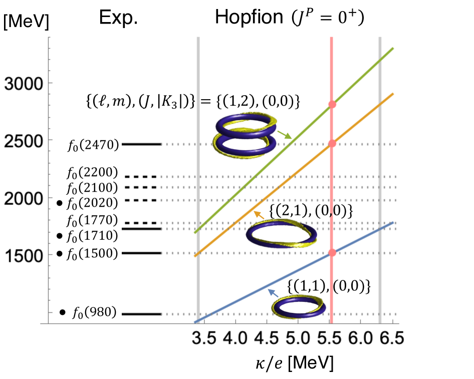
Figure 1: Energy spectra of the Hopfions with $J=0$. On the r.h.s. of the vertical axis, the energies of the Hopfion with the winding numbers $(\ell,m)=(1,1)$, $(2,1)$ and $(1,2)$ are plotted as functions of $\kappa/e$. The red vertical dotted line corresponds to Eq. (5) while the gray vertical dotted lines correspond to $\kappa/e=3.40$ MeV and $6.31$ MeV discussed in Supplemental Material. The profile of each Hopfion is also plotted: the purple isosurface shows the field line with $n_{3}=-1$ representing the Hopfion’s position, and the yellow shows $\bm{n}=(\sqrt{2\mu-\mu^{2}},0,-1+\mu)$ with $\mu=0.1$ representing the linking. On the l.h.s., the mass spectrum of light unflavored mesons with $J^{PC}=0^{++}$ in PDG Workman et al. (2022) is given. The solid (dashed) lines stand for particles with a decay width smaller (larger) than $150$ MeV, and the symbols $\bullet$ indicate established particles.

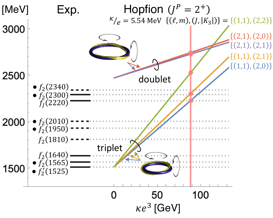
Figure 2: Energy spectra of the Hopfions with $J=2$ for Eq. (5). The Hopfion energies are plotted as functions of $\kappa e^{3}$ to the r.h.s of the vertical axis. On the l.h.s., the mass spectra of light unflavored mesons with $J^{PC}=2^{++}$ collected in PDG Workman et al. (2022) is given. We also included $f_{J}(2220)$ with assuming $J=2$. The red vertical dotted line corresponds to $\kappa e^{3}=88.5$ GeV, where the energy of the first excited state $\{(\ell,m),(J,|K_{3}|)\}=\{(1,1),(2,0)\}$ equals to the mass of $f_{J}(2220)$ as a possible candidate of the tensor glueball.

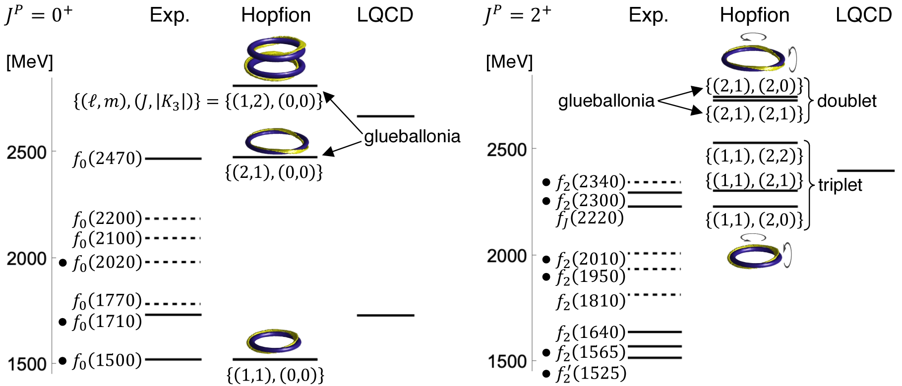
Figure 3: Comparison between the Hopfion energy spectra and the mass spectra of light unflavored mesons listed in PDG Workman et al. (2022) and glueballs predicted by LQCD Morningstar and Peardon (1999). Left panel is for $0^{++}$ and right panel $2^{++}$. The symbol $\bullet$ indicates established particles. We used the values of the coupling constants in Eqs. (5) and (6).

Table 1: Hopfion energy eigenvalues ($E$) with the values of the coupling constants in Eqs. (5) and (6). The last column shows the masses of scalar and tensor mesons, $f_{0}(1500)$, $f_{0}(2470)$, $f_{J=2}(2220)$, $f_{2}(2300)$ and $f_{2}(2340)$ Workman et al. (2022). The mesons used for the fitting are indicated by asterisks. All the states with $Q=2$ are candidates of glueballonia. See the text.

$Q$	$(\ell,m)$	multiplet	$(J,|K_{3}|)$	$E$ [MeV]	Exp. [MeV]
1	(1,1)	singlet	(0,0)	1522	1500∗
			(2,0)	2231	2220∗
		triplet	(2,1)	2306	2300
			(2,2)	2531	2340
2	(2,1)	singlet	(0,0)	2477	2470
		doublet	(2,0)	2749	—
			(2,1)	2732	—
2	(1,2)	singlet	(0,0)	2814	—
			(2,0)	3034	—
		triplet	(2,1)	3108	—
			(2,2)	3330	—

To evaluate the Hopfion energy spectrum, we need to fix the coupling constants. In the length scale $1/\kappa e$, the static mass is proportional to $\kappa/e$ and the quantum correction to $1/\kappa e^{3}$ . Here we set the parameters $\kappa/e$ and $\kappa e^{3}$ by identifying the Hopfions as light unflavored (isosinglet) mesons carrying spin-parity $J^{P}=0^{+}$ and $2^{+}$ listed by the Particle Data Group (PDG) Workman et al. (2022).

Identifying the $Q=1$ Hopfion with $\{(\ell,m),(J,|K_{3}|)\}=\{(1,1),(0,0)\}$ as the scalar meson $f_{0}(1500)$, which is one of the primary candidates for the lowest-lying scalar glueball Morningstar and Peardon (1999), we obtain

$$\kappa/e=5.54~\text{MeV}.$$ (5)

Once the parameter $\kappa/e$ is fixed, the energy spectrum of the Hopfions with $J^{P}=0^{+}$ is fully determined as the classical solution, as shown in Fig. 1. There one observes that the $Q=2$ Hopfion carrying $\{(2,1),(0,0)\}$ with the value (5) acquires the mass extremely close to $f_{0}(2470)$, which is very narrow with the decay width, $75^{+14}_{-12}$ MeV, compared to its large mass Workman et al. (2022). Thus, the parameter set (5) is successful for reproducing the masses of $f_{0}(1500)$ and $f_{0}(2470)$ simultaneously. Besides, we find another $Q=2$ Hopfion with $\{(1,2),(0,0)\}$ with mass 2814 MeV, which has no corresponding state in the PDG list yet. This novel scalar meson is expected to be verified in future experiments.

With the given $\kappa/e$, the masses of Hopfions with $J^{P}=2^{+}$ can also be obtained. They include quantum fluctuations beyond the classical solution. Figure 2 shows the energy spectrum of the $J^{P}=2^{+}$ Hopfions with the value in Eq. (5). The lowest state, the $Q=1$ Hopfion with $\{(1,1),(2,0)\}$, can naturally be identified as the narrowest tensor glueball, $f_{J}(2220)$, with the decay width $23^{+8}_{-7}$ MeV Workman et al. (2022), assuming $J=2$. This results in

$$\kappa e^{3}=88.5~\text{GeV},$$ (6)

leading to the full $2^{+}$ Hopfion energy spectrum. One finds that the energy of another $Q=1$ Hopfion with $\{(1,1),(2,1)\}$ well coincides with the mass of $f_{2}(2300)$. There is also the $Q=1$ Hopfion with $\{(1,1),(2,2)\}$ which may be comparable with $f_{2}(2340)$. Thus, the Hopfion approach predicts the triplet structure, i.e., $f_{J=2}(2220)$, $f_{2}(2300)$ and $f_{2}(2340)$, and all of which are possible candidates of tensor glueballs in contrast to the singlet structures in $0^{+}$. We also find a doublet of $Q=2$ Hopfions with $\{(2,1),(2,1)\}$ and $\{(2,1),(2,0)\}$, which is a genuine prediction of the Hopfion approach and should be experimentally assessed if they would serve as tensor glueballs.

We summarize the Hopfion energy spectra in Table 1. Figure. 3 shows a direct comparison of these results with the masses of scalar and tensor mesons in PDG and the glueball masses predicted in LQCD Morningstar and Peardon (1999). It should be emphasized that in the Hopfion approach the masses of $f_{0}(2470)$, $f_{2}(2300)$ and $f_{2}(2340)$ are determined systematically without any fine-tuning. One may consider other parameter settings, which however turns out to be unfavorable .

The Hopfion approach also provides the interpretation that the heavier scalar glueballs are bound states of the lightest glueballs, i.e., glueballonia Giacosa et al. (2022). The two $Q=2$ Hopfions with $(\ell,m)=(2,1)$ and $(1,2)$ can be identifed as a tightly and a loosely bound glueballonia of masses $2477$ MeV and $2814$ MeV, respectively, possessing the binding energies of $576$ MeV and $230$ MeV calculated in this model. Whereas the former is identified as the known state, $f_{0}(2470)$, the latter is a novel exotic particle.

IV Summary

We developed the Hopfion approach to describe low-lying scalar and tensor glueballs, confronted with the currently available data from experiments and LQCD as well as the QCD phenomenology. Our model predicts that $f_{0}(2470)$ is a tightly bound glueballonium on top of a loosely bound one as a novel scalar state. Thus, the Hopfion approach explains the unnaturally long lifetime of $f_{0}(2470)$, while an observation of the new glueballonium in future measurements would be a critical verification of this approach. We also found several other Hopfions with $Q=1$ and $2$ corresponding to known and unknown glueballs, which are classified into the characteristic multiplet structures anchored to the underlying topology.

The current approach captures the peculiar features to glueballs complying with the existing data from measurements and lattice simulations, while this can be further refined: We used the rigid body quantization for tensor glueballs, whereas the stationary isospinning solutions have been studied beyond the rigid body taking into account the deformation due to rotation Harland et al. (2013); Battye and Haberichter (2013). Including this effect may produce somecorrections to the spectra of tensor glueballs presented in this Letter.

Formation of the glueballonia from two glueballs may be investigated in synergy with relativistic heavy-ion collisions and real time dynamics of Hopfions. Quantum transitions between different glueball states should be studied in the Hopfion approach. Modeling Hopfions coupled to dynamical quarks is also desired to study decays of glueballs into quark-antiquark pairs to be compared with experimental data.

V Acknowledgments

YA is grateful for the kind hospitality at the Instituto de Física de São Carlos of Universidade de São Paulo (IFSC/USP). This work is supported in part by JSPS KAKENHI [Grants No. JP23KJ1881 (YA), No. JP22H01221 (MN)] and the WPI program “Sustainability with Knotted Chiral Meta Matter (SKCM²)” at Hiroshima University. The work of CS was supported partly by the Polish National Science Centre (NCN) under OPUS Grant No. 2022/45/B/ST2/01527. The numerical computations in this paper were run on the “GOVORUN” cluster supported by the LIT, JINR.

Supplemental material

VI I. Explicit form of the classical mass and inertia tensors

In this section, we describe the quantization of rotation modes of Hopfions.

VI.1 Semiclassical quantization

The static energy of the model is invariant under the translation, spatial rotation and isospatial rotation, which is described by the transformation

$$\mathfrak{n}(\bm{x})\to\mathfrak{n}(\bm{x};\bm{X},A,B)\equiv A\mathfrak{n}(R(B)(\bm{x}-\bm{X}))A^{\dagger},$$ (S.1)

where $\bm{X}$ denotes a translation, $A$ is an $SU(2)$ matrix associated with an isospatial rotation, and spatial rotation is represented by

$$R_{jk}(B)=\frac{1}{2}\mathop{Tr}\nolimits\left(\tau_{j}B\tau_{k}B^{\dagger}\right),$$ (S.2)

with an $SU(2)$ matrix $B$. The degeneracy described in Eq. (S.1) is lifted when the theory is quantized. We apply a collective coordinate quantization Adkins et al. (1983); Braaten and Carson (1988); Krusch and Speight (2006); Kondo et al. (2006) implemented by promoting the parameters $\bm{X},A$, and $B$ to the dynamical variable $\bm{X}(t),A(t)$, and $B(t)$, and then by quantizing the dynamical system according to the canonical method. Therefore, we consider a dynamical ansatz of the form

$$\hat{\mathfrak{n}}(\bm{x},t)\equiv A(t)\mathfrak{n}(R(B(t))\bm{x})A(t)^{\dagger},$$ (S.3)

where we have ignored the translational degrees of freedom $\bm{X}(t)$, which means that we quantize a Hopfion in its rest frame. Substituting the ansatz (S.3) into the Lagrangian density in Eq. (1) and integrating over three-dimensional space, one finds the effective Lagrangian

$$L[\hat{\mathfrak{n}}]=T-M_{\mathrm{cl}},$$ (S.4)

where $M_{\mathrm{cl}}$ stands for the static energy of the background field $\mathfrak{n}(\bm{x})$, and the kinetic energy $T$ can be written as

$$T=\frac{1}{2}a_{j}U_{jk}a_{k}-a_{j}W_{jk}b_{k}+\frac{1}{2}b_{j}V_{jk}b_{k},$$ (S.5)

with the inertial tensors $U_{jk},~W_{jk}$ and $V_{jk}$, given below. The variables $a_{j}$ and $b_{j}$ denote angular velocities of isospacial and spacial rotations, respectively, defined as $a_{j}=-i\mathop{Tr}\nolimits(\tau_{j}A^{\dagger}\partial_{t}A),~b_{j}=i\mathop{Tr}\nolimits(\tau_{j}\partial_{t}BB^{\dagger})$. In the length scale $1/\kappa e$, one can write $M_{\mathrm{cl}}=\frac{\kappa}{e}M_{\mathrm{cl}}^{*}$ and $\left(U_{jk},W_{jk},V_{jk}\right)=\frac{1}{\kappa e^{3}}\left(U_{jk}^{*},W_{jk}^{*},V_{jk}^{*}\right)$ with the parameter-free quantities

$$M_{\mathrm{cl}}^{*}=\int d^{3}x\left[\frac{1}{4}\mathop{Tr}\nolimits\left(\partial_{k}\mathfrak{n}\partial_{k}\mathfrak{n}\right)-\frac{1}{32}\mathop{Tr}\nolimits\left[\partial_{j}\mathfrak{n},\partial_{k}\mathfrak{n}\right]^{2}\right],$$ (S.6)

$$U_{jk}^{*}=\int d^{3}x\left[-\frac{1}{8}\mathop{Tr}\nolimits\left([\tau_{j},\mathfrak{n}][\tau_{k},\mathfrak{n}]\right)+\frac{1}{32}\mathop{Tr}\nolimits\left[[\tau_{j},\mathfrak{n}],\partial_{l}\mathfrak{n}][[\tau_{k},\mathfrak{n}],\partial_{l}\mathfrak{n}\right]\right],$$ (S.7)

$$W_{jk}^{*}=i\int d^{3}x\left[\frac{1}{4}\mathop{Tr}\nolimits\left([\tau_{j},\mathfrak{n}]\mathrm{L}_{k}\mathfrak{n}\right)-\frac{1}{16}\mathop{Tr}\nolimits\left[[\tau_{j},\mathfrak{n}],\partial_{l}\mathfrak{n}][\mathrm{L}_{k}\mathfrak{n},\partial_{l}\mathfrak{n}\right]\right],$$ (S.8)

$$V_{jk}^{*}=\int d^{3}x\left[\frac{1}{2}\mathop{Tr}\nolimits\left(\mathrm{L}_{j}\mathfrak{n}~\mathrm{L}_{k}\mathfrak{n}\right)-\frac{1}{8}\mathop{Tr}\nolimits\left[\mathrm{L}_{j}\mathfrak{n},\partial_{l}\mathfrak{n}][\mathrm{L}_{k}\mathfrak{n},\partial_{l}\mathfrak{n}\right]\right],$$ (S.9)

where $\mathrm{L}_{j}=-i\varepsilon_{jkl}x^{k}\partial_{l}$.

VI.2 Angular momentum and the Hamiltonian

The momenta conjugate to the collective coordinate $A$ and $B$ are defined by $\hat{K}_{j}=\frac{\partial L}{\partial a_{j}}$ and $\hat{L}_{j}=\frac{\partial L}{\partial b_{j}}$, respectively. The $\bm{\hat{K}}~(\bm{\hat{L}})$ is the body-fixed isospin (angular momentum) operator. The coordinate-fixed isospin $(\bm{\hat{I}})$ and spin $(\bm{\hat{J}})$ operators are defined through the orthogonal transformation

$$\hat{I}_{j}=-R_{jk}(A)\hat{K}_{k},\qquad\hat{J}_{j}=-R_{kj}(B)\hat{L}_{k}\,.$$ (S.10)

These relations between the body-fixed and coordinate-fixed operators yield $\bm{\hat{K}}^{2}=\bm{\hat{I}}^{2},~\bm{\hat{L}}^{2}=\bm{\hat{J}}^{2}$. The Hamiltonian is defined through the Legendre transformation as

$$H=\hat{K}_{j}a_{j}+\hat{L}_{j}b_{j}-L.$$ (S.11)

VI.3 Axial symmetric ansatz

For simplicity, we restrict ourselves to considering the axially symmetric Hopfions. It is well known that Hopfion solutions with topological charges $Q=1,2$ have an axial symmetry Gladikowski and Hellmund (1997); Battye and Sutcliffe (1998). To describe axially symmetric Hopfions, we employ an ansatz of the form

$$\bm{n}=(\phi_{1}\cos(\ell\theta)-\phi_{2}\sin(\ell\theta),\phi_{1}\sin(\ell\theta)+\phi_{2}\cos(\ell\theta),\phi_{3}),$$ (S.12)

where $l$ is an integer and $\bm{\phi}=(\phi_{1},\phi_{2},\phi_{3})$ is a three-component unit vector depending only on $(\rho,z)$, with the cylindrical coordinates $(\rho,\theta,z)$. The boundary condition for $\bm{\phi}$ is

$$\bm{\phi}(0,z)=\bm{\phi}(\rho,z)|_{\rho^{2}+z^{2}\to\infty}=(0,0,1).$$ (S.13)

Due to the axial symmetry, all off-diagonal components of the inertia tensors vanish, except for the case where $\ell=\pm 1$, in which $W_{12}=\ell W_{21}\neq 0$. The diagonal components hold the following relations:

$$U_{11}=U_{22},~~V_{11}=V_{22},$$ (S.14)

$$V_{33}=\ell W_{33}=\ell^{2}U_{33}.$$ (S.15)

In addition, one finds that $U_{11}=U_{22}$ diverges under the boundary condition. As a result, the Hamiltonian can be cast into a simple form

$$H=M_{\mathrm{cl}}+\frac{1}{2V_{11}}\bm{\hat{L}}^{2}+\frac{1}{2}\left(\frac{1}{U_{33}}-\frac{\ell^{2}}{V_{11}}\right)\hat{K}_{3}^{2}\ .$$ (S.16)

The relation (S.15) leads to a constraint on the physical Hilbert space of the form

$$\left(\hat{L}_{3}-\ell\hat{K}_{3}\right)\left|{\mathrm{phys}}\right>=0,$$ (S.17)

which gives a selection rule for possible glueball states.

VI.4 The energy eigenvalues and wavefunction

Since this Hamiltonian has the same form as that of a symmetrical top, the energy eigenvalues can be given by

$$E=\frac{\kappa}{e}M_{\mathrm{cl}}^{*}+\frac{\kappa e^{3}}{2}\left\{\frac{J(J+1)}{V_{11}^{*}}+\left(\frac{1}{U_{33}^{*}}-\frac{\ell^{2}}{V_{11}^{*}}\right)K_{3}^{2}\right\}.$$ (S.18)

The eigenstate is given by a superposition of the basis $\left|{J,J_{3},L_{3}}\right>\left|{I,I_{3},K_{3}}\right>$ as

$$\left|{\psi}\right>=\displaystyle{\sum_{I\geq|K_{3}|}\sum_{I_{3},J_{3}}}C^{I}_{I_{3},J_{3}}\left|{J,J_{3},L_{3}}\right>\left|{I,I_{3},K_{3}}\right>,$$ (S.19)

where $|J_{3}|,|L_{3}|\leq J$ and $|I_{3}|,|K_{3}|\leq I$, and $C_{I_{3},J_{3}}$ are normalization constants. In addition, the quantum numbers satisfy the constraint $L_{3}=\ell K_{3}$, which stems from Eq. (S.17). Since the states $\left|{J,J_{3},L_{3}}\right>$ and $\left|{I,I_{3},K_{3}}\right>$ are eigenstates of a symmetric top, one can write

$$\left<{A}|{I,I_{3},K_{3}}\right>\propto D^{I}_{I_{3}K_{3}}(\alpha_{1},\alpha_{2},\alpha_{3}),\qquad\left<{B}|{J,J_{3},L_{3}}\right>\propto D^{J}_{J_{3}L_{3}}(\beta_{1},\beta_{2},\beta_{3}),$$ (S.20)

with the Wigner $D$-functions, where $\alpha_{i}$ and $\beta_{i}$ are Euler angles in isospace and real space, respectively The wave function can be written as

$$\psi\equiv\left<{A,B}|{\psi}\right>$$

$$=\sum_{I_{3},J_{3}}C_{I_{3},J_{3}}\left<{A}|{I,I_{3},K_{3}}\right>\left<{B}|{J,J_{3},L_{3}}\right>$$

$$\propto\sum_{I\geq|K_{3}|}\sum_{I_{3},J_{3}}C^{I}_{I_{3},J_{3}}D^{J}_{J_{3}L_{3}}(\beta_{1},\beta_{2},\beta_{3})D^{I}_{I_{3}K_{3}}(\alpha_{1},\alpha_{2},\alpha_{3})\ .$$ (S.21)

Table S1: Classical masses and inertia tensors of Hopfions ($Q=\ell m$) as dimensionless quantities.

$Q$	$(\ell,m)$	$M_{\mathrm{cl}}^{*}$	$V_{11}^{*}$	$U_{33}^{*}$
1	(1,1)	274.79	372.17	227.78
2	(2,1)	447.20	968.33	267.72
2	(1,2)	508.16	1203.1	398.09

VII II. Numerical procedure

In this section, we explain the numerical procedure for constructing Hopfion solutions. To describe axially symmetric Hopfions, we employ an ansatz of the form

$$\bm{n}=(\phi_{1}\cos(\ell\theta)-\phi_{2}\sin(\ell\theta),\phi_{1}\sin(\ell\theta)+\phi_{2}\cos(\ell\theta),\phi_{3}),$$ (S.22)

where $\ell$ is an integer and $\bm{\phi}=(\phi_{1},\phi_{2},\phi_{3})$ is a three-component unit vector depending only on $(\rho,z)$, with the cylindrical coordinates $(\rho,\theta,z)$. The boundary condition for $\bm{\phi}$ is

$$\bm{\phi}(0,z)=\bm{\phi}(\rho,z)|_{\rho^{2}+z^{2}\to\infty}=(0,0,1).$$ (S.23)

To evaluate the classical mass and inertia tensors, we numerically construct Hopfion solutions. We employ the following initial configuration appropriate to describing Hopfions of torus shape Sutcliffe (2007):

$$\bm{\phi}=\frac{1}{1+F_{1}^{2}+F_{2}^{2}}(2F_{1},-2F_{2},F_{1}^{2}+F_{2}^{2}-1),$$ (S.24)

where

$$F_{1}+iF_{2}=\frac{\left(\cos f(\rho)+i\dfrac{z}{r}\sin f(\rho)\right)^{m}}{\left(\dfrac{\rho}{r}\sin f(\rho)\right)^{\ell}},$$ (S.25)

with an integer $m$ and $r=\sqrt{\rho^{2}+z^{2}}$. The function $f(\rho)$ is chosen to satisfy the boundary condition $f(0)=\pi$ and $f(\infty)=0$. The initial configuration possesses the Hopf charge $Q=\ell m$. We numerically construct Hopfion solutions using a nonlinear conjugate gradient method with a fourth-order finite difference scheme. The grid in the $\rho\text{-}z$ plane contains $75\times 150$ points with a lattice spacing of $0.1$ in the length scale $1/\kappa e$. The value of the classical mass and inertia tensors that the numerical solution possesses are listed in Table S1.

VIII III. Results with other parameter settings

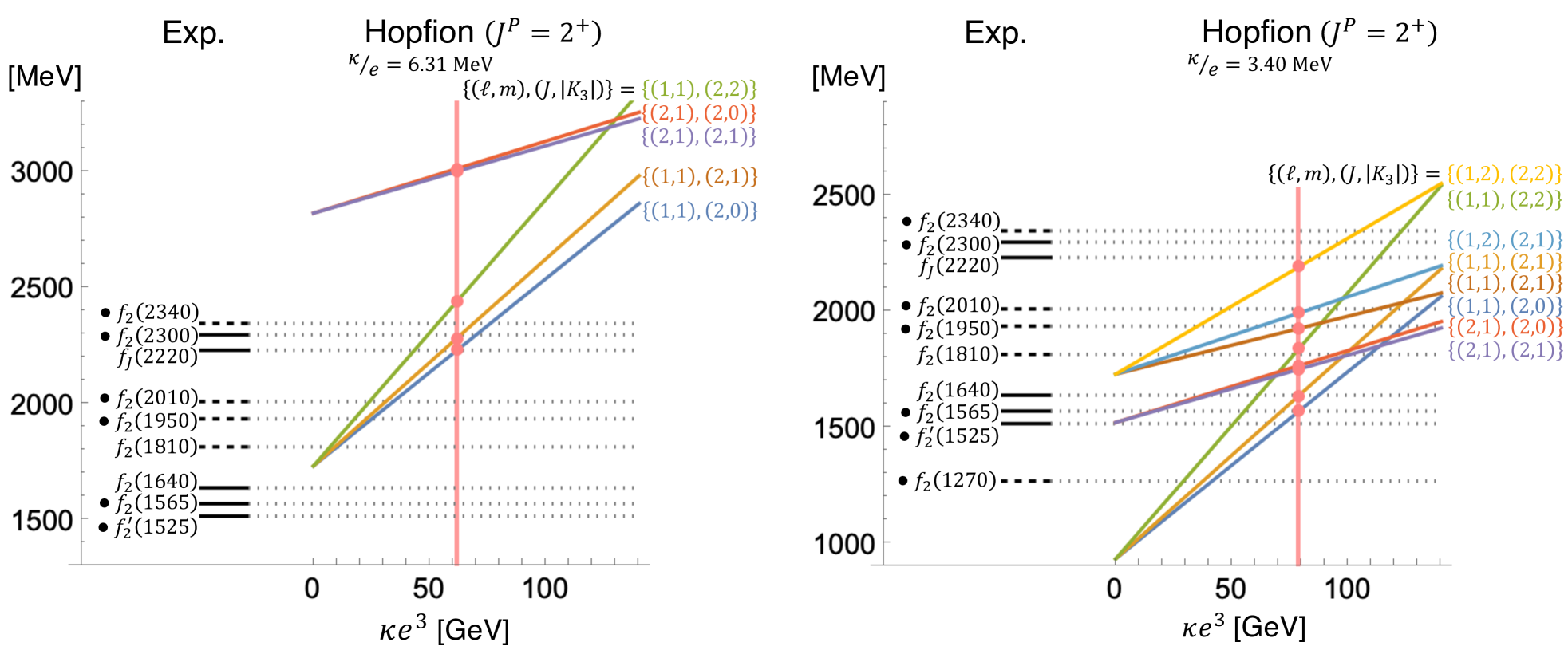
Figure S1: The energy spectra of the Hopfions with $J=2$ for $\kappa/e=3.40$ MeV (Case 2; left panel) and $\kappa/e=6.31$ MeV (Case 3; right panel). By the red vertical dotted lines, the value of $\kappa e^{3}$ are indicated for which the energy of the $Q=1$ Hopfion with $\{(1,1),(2,0)\}$ is assigned to $f_{2}(1565)$ in Case 2 and $f_{J=2}(2220)$ in Case 3. Notice that the $Q=1$ Hopfion with $\{(1,1),(0,0)\}$ is assigned to $f_{0}(1500)$ in Case 2 and to $f_{0}(1710)$ in Case 3, as shown in Fig. 1.

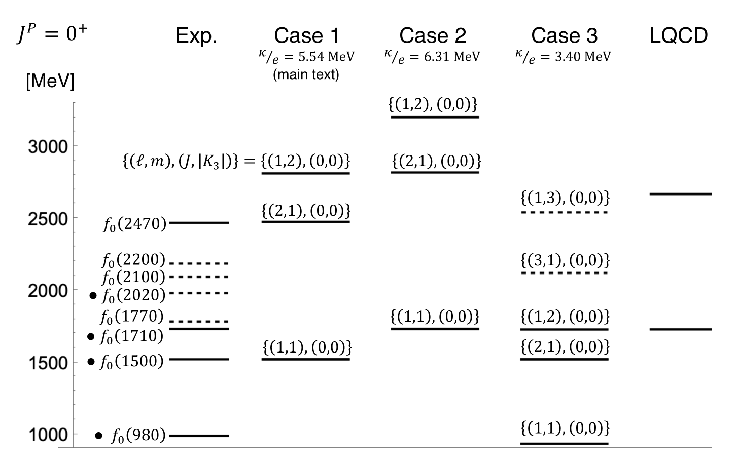
Figure S2: Comparison of Hopfion energy spectra for $J^{P}=0^{+}$ case with three different choices of coupling constants (Case 1, 2 and 3). The states used to calibrate the parameters are represented in red. Hopfions with $(\ell,m)=(3,1)$ and $(1,3)$ are constructed by 3D full simulation, which is different from the others because they are not axially symmetric. On the l.h.s of the vertical axis, the mass spectra of light unflavored mesons collected in PDG Workman et al. (2022) is given. The LQCD data was taken from Ref. Morningstar and Peardon (1999). The solid (dashed) line stands for particles with a decay width smaller (larger) than $150$ MeV, and the symbol $\bullet$ indicates established particles.

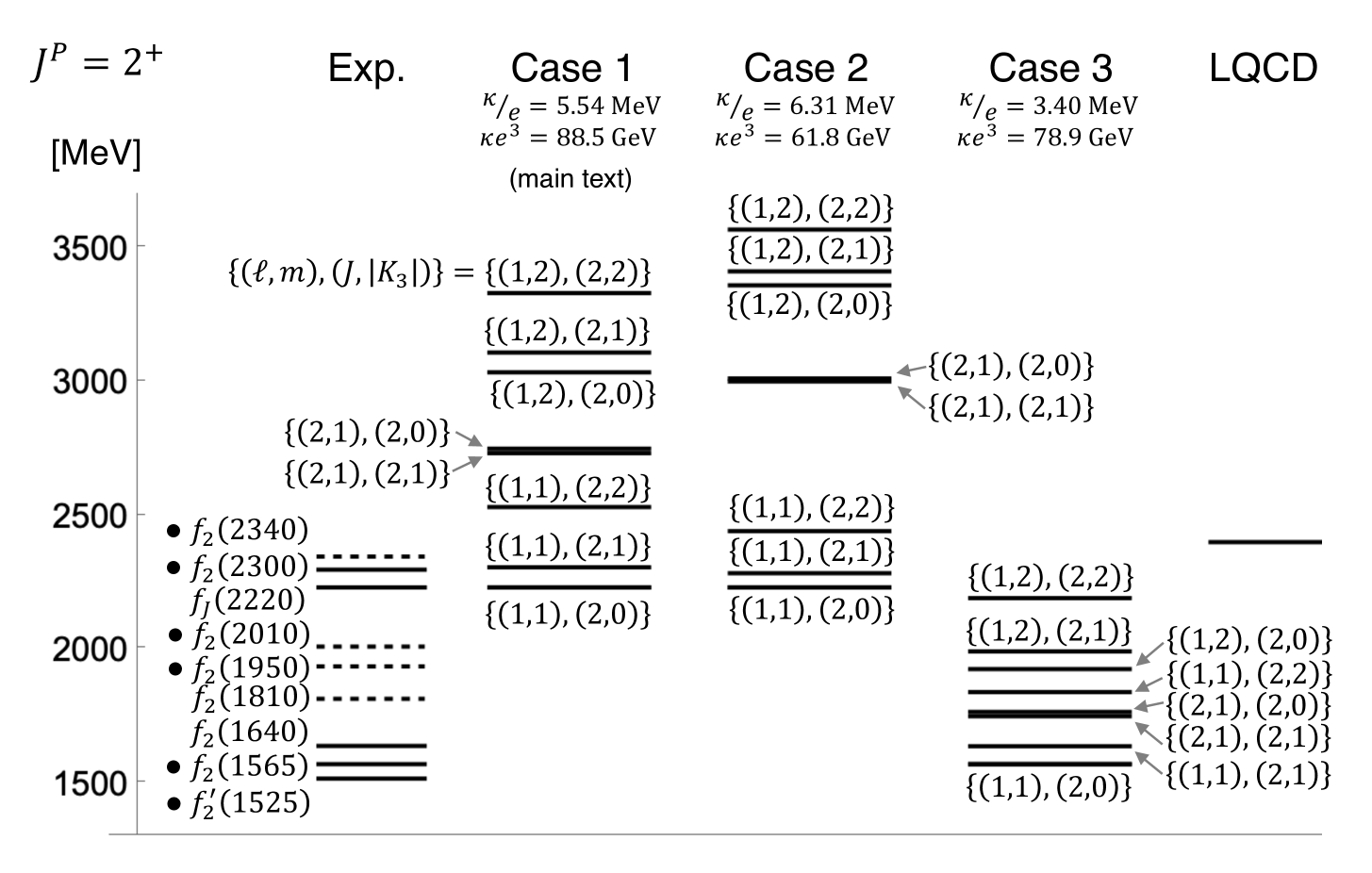
Figure S3: The $J^{P}=2^{+}$ case for Fig. S2.

Table S2: Hopfion energies in unit of MeV for Cases 1, 2 and 3, see Eqs. (S.30)-(S.36). The parameters are: $\kappa/e=5.54$ MeV and $\kappa e^{3}=88.5$ GeV in Case 1, $\kappa/e=6.31$ MeV and $\kappa e^{3}=61.8$ GeV in Case 2, and $\kappa/e=3.40$ MeV and $\kappa e^{3}=78.9$ GeV in Case 3. The Hopfions used for the fitting to experimental data are indicated by daggers.

$(\ell,m)$	$(J,|K_{3}|)$		Case 1	Case 2	Case 3
(1,1)	(0,0)		1522†	1733†	935
	(2,0)		2231†	2231†	1571†
	(2,1)		2306	2283	1638
	(2,2)		2531	2441	1840
(2,1)	(0,0)		2477	2820	1522†
	(2,0)		2749	3011	1766
	(2,1)		2732	3000	1750
(1,2)	(0,0)		2814	3204	1729
	(2,0)		3034	3359	1926
	(2,1)		3108	3411	1992
	(2,2)		3330	3567	2191

In the main text, we have considered the Hopfion energy spectra for the parameter sets in Eqs. (5) and (6). We call this parameter set Case 1. There, focusing on the importance of $f_{0}(1500)$ in $J^{P}=0^{+}$, we have considered it as the $Q=1$ Hofpion and set the parameter value $\kappa/e=5.54$ MeV in Eq. (5), simultaneously reproducing the masses of $f_{0}(2430)$ as the $Q=2$ Hopfion. We have also regarded $f_{J=2}(2220)$ in $J^{P}=2^{+}$ as the $Q=1$ Hopfion by setting the parameter value $\kappa e^{3}=88.5$ GeV in Eq. (6), and have found the triplet structure, i.e., $f_{J=2}(2220)$, $f_{2}(2300)$ and $f_{2}(2340)$. However, one may consider that Case 1 is not the only possible parameter set. Here, we investigate the other parameter settings and explore the possible energy spectra of Hopfions.

It was reported in the holographic QCD approach that $f_{0}(1710)$ can be regarded as a glueball, while $f_{0}(1500)$ is unlikely to be Brünner et al. (2015). Such case can be realized by the Hopfion approach by setting

$$\kappa/e=6.31~\text{MeV}\mbox{ : Case 2},$$ (S.26)

as shown at the grey vertical line on the right in Fig. 1. On the other hand, one can reproduce $f_{0}(1500)$ and $f_{0}(1710)$ simultaneously by setting

$$\kappa/e=3.40~\text{MeV}\mbox{ : Case 3},$$ (S.27)

as shown at the grey vertical line on the left in Fig. 1. In this case, however, it is inevitable for $f_{0}(980)$ to be identified as a glueball, which is different from the conventional understanding that $f_{0}(980)$ is an excited quark-antiquark state with a relative $P$-wave component (see, e.g., Refs. Donoghue et al. (2014); Amsler and Tornqvist (2004)). Indeed, this can be understood from the existence of an isotriplet scalar meson $a_{0}(980)$ as an isospin partner of $f_{0}(980)$. In the present study, we call those parameter settings Cases 2 and 3 compared with Case 1, where $f_{0}(1500)$ is excluded in Case 2 and $f_{0}(980)$ appears as a glueball in Case 3. Nevertheless, those parameter settings exhibit interesting behaviors in the energy spectra of Hopfions. The attempted parameter sets are summarized below:

$$\text{Case 1:}\begin{array}[]{ll}&\{(1,1),(0,0)\}~~\leftrightarrow~~f_{0}(1500)\\ &\{(1,1),(2,0)\}~~\leftrightarrow~~f_{J=2}(2220)\end{array}~~\leftrightarrow~~\kappa/e=5.54\text{~MeV,~~}\kappa e^{3}=88.5\text{~GeV},$$ (S.30)

$$\text{Case 2:}\begin{array}[]{ll}&\{(1,1),(0,0)\}~~\leftrightarrow~~f_{0}(1710)\\ &\{(1,1),(2,0)\}~~\leftrightarrow~~f_{J=2}(2220)\end{array}~~\leftrightarrow~~\kappa/e=6.31\text{~MeV,~~}\kappa e^{3}=61.8\text{~GeV},$$ (S.33)

$$\text{Case 3:}\begin{array}[]{ll}&\{(2,1),(0,0)\}~~\leftrightarrow~~f_{0}(1500)\\ &\{(1,1),(2,0)\}~~\leftrightarrow~~f_{2}(1565)\end{array}~~~~~\leftrightarrow~~\kappa/e=3.40\text{~MeV,~~}\kappa e^{3}=78.9\text{~GeV}.$$ (S.36)

Here, Case 1 discussed in the main text is shown for convenience in comparison to Cases 2 and 3. We comment that $f_{2}(1430)$ and $f_{2}^{\prime}(1525)$ are not taken into account as the candidate of glueballs despite of their smaller masses in our fittings, because they are considered to belong to radially excited quark-antiquark states with relative $P$-wave component ($1^{3}P_{2}$: principal number (node number) 1, total spin 1, $P$-wave and total angular momentum 2) Amsler and Tornqvist (2004).

For Cases 2 and 3, the dependence on $\kappa e^{3}$ in the Hopfion energy spectra are shown in Fig. S1. Similarly to Case 1, the values of $\kappa e^{3}$ in Cases 2 and 3 are obtained by the fitting to the observed tensor mesons, as discussed in details below.

In Case 2, we obtain $\kappa/e^{3}=61.8$ GeV by assigning the $Q=1$ Hopfion with $\{(1,1),(2,0)\}$ to $f_{J=2}(2220)$ in $J^{P}=2^{+}$, as indicated in the left panel of Fig. S1. Here $f_{J=2}(2220)$ is chosen because it has the decay width $23^{+8}_{-7}$ MeV, relatively small number irrespective to its large mass. This is the same assignment as Case 1 discussed in the main text. As a result, we obtain the Hopfion energy spectra in Figs. S2 and S3 and the numerical values in Table S2. It is interesting to see that $f_{2}(2300)$ and $f_{2}(2340)$ are comparable with the $Q=1$ Hopfions with $\{(1,1),(2,1)\}$ and $\{(1,1),(2,2)\}$, respectively, and hence $f_{J=2}(2220)$, $f_{2}(2300)$ and $f_{2}(2340)$ can be regarded as a triplet, as discussed in Case 1. Similarly to Case 1, we also predict new tensor glueballs as the $Q=2$ doublet Hopfions with $\{(2,1),(2,1)\}$ and $\{(2,1),(2,0)\}$.

In Case 3, we obtain $\kappa/e^{3}=78.9$ GeV by assigning the $Q=1$ Hopfion with $\{(1,1),(2,0)\}$ to $f_{2}(1565)$ in $J^{P}=2^{+}$, as indicated in the right panel in Fig. S1. In this fitting, we regard $f_{2}(1565)$, $f_{2}(1640)$ and $f_{2}(1810)$ as the triplet. This assignment is reasonable because the ratio of the mass splittings among these tensor mesons, $M_{f_{2}(1640)}-M_{f_{2}(1565)}:M_{f_{2}(1810)}-M_{f_{2}(1565)}=1:3.6$, is close to the ratio of energy splitting of the Hopfions, $1:4$, estimated from the mass formula in Eq. (4). Note, however, that $f_{2}(1565)$, $f_{2}(1640)$ and $f_{2}(1810)$ have the decay widths $132\pm{23}$ MeV, $100^{+60}_{-40}$ MeV and $197\pm 22$ MeV, respectively, the order of hundred MeV.

As summarized in Figs. S2 and S3 and Table S2, in Case 3, there are many excited states in $J^{P}=0^{+}$ and $2^{+}$. In $J^{P}=0^{+}$, we find that the $Q=2$ Hopfions with $\{(2,1),(0,0)\}$ and $\{(1,2),(0,0)\}$ are comparable with $f_{0}(1500)$ and $f_{0}(1710)$, respectively. We also find that the $Q=3$ Hopfions with $\{(3,1),(0,0)\}$ is close either to $f_{0}(2020)$, $f_{0}(2100)$ or $f_{0}(2200)$. More interestingly, we find that the $Q=3$ Hopfion with $\{(1,3),(0,0)\}$ is near $f_{0}(2470)$, a narrow scalar meson, which has been identified to be $\{(2,1),(0,0)\}$ in Cases 1 and 2. In $J^{P}=2^{+}$, similarly, the correspondence between the Hopfions and the tensor mesons is seen. Similarly to Case 1 and 2, we find the doublet, i.e., the $Q=2$ Hopfion with $\{(2,1),(2,1)\}$ and $\{(2,1),(2,0)\}$ in Fig. S1. It is particularly interesting that the $Q=2$ Hopfion with $\{(1,2),(2,2)\}$ is near $f_{J=2}(2220)$, a narrow tensor meson, which has been discussed in Cases 1 and 2. Thus, $f_{J=2}(2220)$ is assigned to the triplet, i.e., $Q=2$ Hopfion with $\{(1,2),(2,0)\}$, $\{(1,2),(2,1)\}$ and $\{(1,2),(2,2)\}$, as presented in Fig. S1. This assignment is different from that in Cases 1 and 2.

References

- Clay Mathematics Institute (2000) Clay Mathematics Institute, “The millennium prize problems,” (2000).
- Fritzsch and Minkowski (1975) H. Fritzsch and P. Minkowski, Il Nuovo Cimento A (1965-1970) 30, 393 (1975).
- Jaffe et al. (1986) R. L. Jaffe, K. Johnson, and Z. Ryzak, Annals Phys. 168, 344 (1986).
- Close (1991) F. Close, Nature 349, 368 (1991).
- Klempt and Zaitsev (2007) E. Klempt and A. Zaitsev, Phys. Rept. 454, 1 (2007), arXiv:0708.4016 [hep-ph] .
- Mathieu et al. (2009) V. Mathieu, N. Kochelev, and V. Vento, Int. J. Mod. Phys. E 18, 1 (2009), arXiv:0810.4453 [hep-ph] .
- Crede and Meyer (2009a) V. Crede and C. A. Meyer, Prog. Part. Nucl. Phys. 63, 74 (2009a), arXiv:0812.0600 [hep-ex] .
- Greensite (2011) J. Greensite, An introduction to the confinement problem, Vol. 821 (2011).
- Ochs (2013) W. Ochs, J. Phys. G 40, 043001 (2013), arXiv:1301.5183 [hep-ph] .
- Shepherd et al. (2016) M. R. Shepherd, J. J. Dudek, and R. E. Mitchell, Nature 534, 487 (2016), arXiv:1802.08131 [hep-ph] .
- Llanes-Estrada (2021) F. J. Llanes-Estrada, Eur. Phys. J. ST 230, 1575 (2021), arXiv:2101.05366 [hep-ph] .
- Chen et al. (2023a) H.-X. Chen, W. Chen, X. Liu, Y.-R. Liu, and S.-L. Zhu, Rept. Prog. Phys. 86, 026201 (2023a), arXiv:2204.02649 [hep-ph] .
- Vadacchino (2023) D. Vadacchino, in 39th International Symposium on Lattice Field Theory (2023) arXiv:2305.04869 [hep-lat] .
- Morningstar (2024) C. Morningstar, PoS LATTICE2024, 004 (2024), arXiv:2502.02547 [hep-lat] .
- Johnson and Teper (1998) R. W. Johnson and M. Teper, Nucl. Phys. B Proc. Suppl. 63, 197 (1998), arXiv:hep-lat/9709083 .
- Michael and Teper (1989) C. Michael and M. Teper, Nucl. Phys. B 314, 347 (1989).
- Bali et al. (1993) G. S. Bali, K. Schilling, A. Hulsebos, A. C. Irving, C. Michael, and P. W. Stephenson (UKQCD), Phys. Lett. B 309, 378 (1993), arXiv:hep-lat/9304012 .
- Sexton et al. (1995) J. Sexton, A. Vaccarino, and D. Weingarten, Phys. Rev. Lett. 75, 4563 (1995), arXiv:hep-lat/9510022 .
- Morningstar and Peardon (1999) C. J. Morningstar and M. J. Peardon, Phys. Rev. D 60, 034509 (1999), arXiv:hep-lat/9901004 .
- Johnson and Teper (2002) R. W. Johnson and M. J. Teper, Phys. Rev. D 66, 036006 (2002), arXiv:hep-ph/0012287 .
- Liu and Wu (2002) D. Q. Liu and J. M. Wu, Mod. Phys. Lett. A 17, 1419 (2002), arXiv:hep-lat/0105019 .
- Meyer and Teper (2005) H. B. Meyer and M. J. Teper, Phys. Lett. B 605, 344 (2005), arXiv:hep-ph/0409183 .
- Chen et al. (2006) Y. Chen et al., Phys. Rev. D 73, 014516 (2006), arXiv:hep-lat/0510074 .
- Loan and Ying (2006) M. Loan and Y. Ying, Prog. Theor. Phys. 116, 169 (2006), arXiv:hep-lat/0603030 .
- Gregory et al. (2012) E. Gregory, A. Irving, B. Lucini, C. McNeile, A. Rago, C. Richards, and E. Rinaldi, JHEP 10, 170 (2012), arXiv:1208.1858 [hep-lat] .
- Brett et al. (2020) R. Brett, J. Bulava, D. Darvish, J. Fallica, A. Hanlon, B. Hörz, and C. Morningstar, AIP Conf. Proc. 2249, 030032 (2020), arXiv:1909.07306 [hep-lat] .
- Athenodorou and Teper (2020) A. Athenodorou and M. Teper, JHEP 11, 172 (2020), arXiv:2007.06422 [hep-lat] .
- Chen et al. (2023b) F. Chen, X. Jiang, Y. Chen, K.-F. Liu, W. Sun, and Y.-B. Yang, Chin. Phys. C 47, 063108 (2023b), arXiv:2111.11929 [hep-lat] .
- Sakai and Sasaki (2023) K. Sakai and S. Sasaki, Phys. Rev. D 107, 034510 (2023), arXiv:2211.15176 [hep-lat] .
- Isgur and Paton (1985) N. Isgur and J. E. Paton, Phys. Rev. D 31, 2910 (1985).
- Kuti (1999) J. Kuti, Nucl. Phys. B Proc. Suppl. 73, 72 (1999), arXiv:hep-lat/9811021 .
- Jaffe and Johnson (1976) R. L. Jaffe and K. Johnson, Phys. Lett. B 60, 201 (1976).
- Barnes (1981) T. Barnes, Z. Phys. C 10, 275 (1981).
- Cornwall and Soni (1983) J. M. Cornwall and A. Soni, Phys. Lett. B 120, 431 (1983).
- Witten (1998) E. Witten, Adv. Theor. Math. Phys. 2, 505 (1998), arXiv:hep-th/9803131 .
- Sakai and Sugimoto (2005) T. Sakai and S. Sugimoto, Prog. Theor. Phys. 113, 843 (2005), arXiv:hep-th/0412141 .
- Csaki et al. (1999) C. Csaki, H. Ooguri, Y. Oz, and J. Terning, JHEP 01, 017 (1999), arXiv:hep-th/9806021 .
- de Mello Koch et al. (1998) R. de Mello Koch, A. Jevicki, M. Mihailescu, and J. P. Nunes, Phys. Rev. D 58, 105009 (1998), arXiv:hep-th/9806125 .
- Brower et al. (2000) R. C. Brower, S. D. Mathur, and C.-I. Tan, Nucl. Phys. B 587, 249 (2000), arXiv:hep-th/0003115 .
- Amador and Caceres (2004) X. Amador and E. Caceres, JHEP 11, 022 (2004), arXiv:hep-th/0402061 .
- Colangelo et al. (2007) P. Colangelo, F. De Fazio, F. Jugeau, and S. Nicotri, Phys. Lett. B 652, 73 (2007), arXiv:hep-ph/0703316 .
- Hashimoto et al. (2008) K. Hashimoto, C.-I. Tan, and S. Terashima, Phys. Rev. D 77, 086001 (2008), arXiv:0709.2208 [hep-th] .
- Forkel (2008) H. Forkel, Phys. Rev. D 78, 025001 (2008), arXiv:0711.1179 [hep-ph] .
- Miranda et al. (2010) A. S. Miranda, C. A. Ballon Bayona, H. Boschi-Filho, and N. R. F. Braga, Nucl. Phys. B Proc. Suppl. 199, 107 (2010), arXiv:0910.4319 [hep-th] .
- Brünner et al. (2015) F. Brünner, D. Parganlija, and A. Rebhan, Phys. Rev. D 91, 106002 (2015), [Erratum: Phys.Rev.D 93, 109903 (2016)], arXiv:1501.07906 [hep-ph] .
- Brünner and Rebhan (2015) F. Brünner and A. Rebhan, Phys. Rev. Lett. 115, 131601 (2015), arXiv:1504.05815 [hep-ph] .
- Rodrigues Filho (2021) C. Rodrigues Filho, Braz. J. Phys. 51, 788 (2021), arXiv:2011.12689 [hep-th] .
- Ablikim et al. (2024) M. Ablikim et al. (BESIII), Phys. Rev. Lett. 132, 181901 (2024), arXiv:2312.05324 [hep-ex] .
- She et al. (2024) Z.-L. She, A.-K. Lei, W.-C. Zhang, Y.-L. Yan, D.-M. Zhou, H. Zheng, and B.-H. Sa, (2024), arXiv:2407.07661 [hep-ph] .
- Liu (2025) B. Liu (BESIII), PoS ICHEP2024, 490 (2025).
- Crede and Meyer (2009b) V. Crede and C. Meyer, Prog. Part. Nucl. Phys. 63, 74 (2009b), arXiv:0812.0600 [hep-ex] .
- Faddeev and Niemi (1997) L. D. Faddeev and A. J. Niemi, Nature 387, 58 (1997).
- Faddeev and Niemi (1999a) L. D. Faddeev and A. J. Niemi, Phys. Rev. Lett. 82, 1624 (1999a).
- Faddeev et al. (2004) L. Faddeev, A. J. Niemi, and U. Wiedner, Phys. Rev. D 70, 114033 (2004).
- Kondo et al. (2006) K.-I. Kondo, A. Ono, A. Shibata, T. Shinohara, and T. Murakami, J. Phys. A 39, 13767 (2006).
- Skyrme (1961) T. H. R. Skyrme, Proc. Roy. Soc. Lond. A 260, 127 (1961).
- Skyrme (1962) T. H. R. Skyrme, Nucl. Phys. 31, 556 (1962).
- Volovik and Mineev (1977) G. E. Volovik and V. P. Mineev, Soviet Journal of Experimental and Theoretical Physics 46, 401 (1977).
- Volovik (2009) G. E. Volovik, The Universe in a helium droplet, International Series of Monographs on Physics (Oxford Scholarship Online, 2009).
- Babaev et al. (2002) E. Babaev, L. D. Faddeev, and A. J. Niemi, Phys. Rev. B 65, 100512 (2002), arXiv:cond-mat/0106152 .
- Rybakov et al. (2019) F. N. Rybakov, J. Garaud, and E. Babaev, Phys. Rev. B 100, 094515 (2019), arXiv:1807.02509 [cond-mat.supr-con] .
- Kawaguchi et al. (2008) Y. Kawaguchi, M. Nitta, and M. Ueda, Phys. Rev. Lett. 100, 180403 (2008), [Erratum: Phys.Rev.Lett. 101, 029902 (2008)], arXiv:0802.1968 [cond-mat.other] .
- Hall et al. (2016) D. Hall, M. Ray, and K. Tiurev et.al., Nature Phys 12, 478 (2016).
- Ollikainen et al. (2019) T. Ollikainen, A. Blinova, M. Möttönen, and D. S. Hall, Phys. Rev. Lett. 123, 163003 (2019), arXiv:1908.01285 [cond-mat.quant-gas] .
- Chen et al. (2013) B. G.-g. Chen, P. J. Ackerman, G. P. Alexander, R. D. Kamien, and I. I. Smalyukh, Phys. Rev. Lett. 110, 237801 (2013).
- Ackerman et al. (2015) P. Ackerman, J. van de Lagemaat, and I. Smalyukh, Nat. Comm. 6, 6012 (2015).
- Ackerman and Smalyukh (2017a) P. Ackerman and I. Smalyukh, Nat. Mater. 16, 426 (2017a).
- Ackerman and Smalyukh (2017b) P. Ackerman and I. Smalyukh, Phys. Rev. X 7, 011006 (2017b).
- Tai et al. (2018) J.-S. Tai, P. Ackerman, and I. Smalyukh, PNAS 115, 921 (2018).
- Tai and Smalyukh (2019) J.-S. B. Tai and I. I. Smalyukh, Science 365, 1449â1453 (2019).
- Smalyukh (2020) I. I. Smalyukh, Rept. Prog. Phys. 83, 106601 (2020).
- Wu and Smalyukh (2022) J.-S. Wu and I. I. Smalyukh, Hopfions, heliknotons, skyrmions, torons and both abelian and nonabelian vortices in chiral liquid crystals (Taylor & Francis, 2022).
- Sutcliffe (2017) P. Sutcliffe, Phys. Rev. Lett. 118, 247203 (2017), arXiv:1705.10966 [cond-mat.mes-hall] .
- Sutcliffe (2018) P. Sutcliffe, J. Phys. A 51, 375401 (2018), arXiv:1806.06458 [cond-mat.mes-hall] .
- Kent et al. (2021) N. Kent et al., Nature Commun. 12, 1562 (2021), arXiv:2010.08674 [cond-mat.mes-hall] .
- Trautman (1977) A. Trautman, Int. J. Theor. Phys. 16, 561 (1977).
- Ranada (1989) A. F. Ranada, Lett. Math. Phys. 18, 97 (1989).
- Kedia et al. (2013) H. Kedia, I. Bialynicki-Birula, D. Peralta-Salas, and W. T. M. Irvine, Phys. Rev. Lett. 111, 150404 (2013), arXiv:1302.0342 [math-ph] .
- Arrayás et al. (2017) M. Arrayás, D. Bouwmeester, and J. L. Trueba, Phys. Rept. 667, 1 (2017).
- Giacosa et al. (2022) F. Giacosa, A. Pilloni, and E. Trotti, Eur. Phys. J. C 82, 487 (2022), arXiv:2110.05582 [hep-ph] .
- Shabanov (1999a) S. V. Shabanov, Phys. Lett. B 458, 322 (1999a), arXiv:hep-th/9903223 .
- Shabanov (1999b) S. V. Shabanov, Phys. Lett. B 463, 263 (1999b), arXiv:hep-th/9907182 .
- Faddeev and Niemi (2002) L. D. Faddeev and A. J. Niemi, Phys. Lett. B 525, 195 (2002).
- Gies (2001) H. Gies, Phys. Rev. D 63, 125023 (2001), arXiv:hep-th/0102026 .
- Langmann and Niemi (1999) E. Langmann and A. J. Niemi, Phys. Lett. B 463, 252 (1999), arXiv:hep-th/9905147 .
- Faddeev and Niemi (1999b) L. D. Faddeev and A. J. Niemi, Phys. Lett. B 449, 214 (1999b).
- Faddeev and Niemi (1999c) L. D. Faddeev and A. J. Niemi, Phys. Lett. B 464, 90 (1999c), arXiv:hep-th/9907180 .
- Kondo et al. (2008) K.-I. Kondo, T. Shinohara, and T. Murakami, Prog. Theor. Phys. 120, 1 (2008), arXiv:0803.0176 [hep-th] .
- Evslin et al. (2011) J. Evslin, S. Giacomelli, K. Konishi, and A. Michelini, JHEP 06, 094 (2011), arXiv:1103.5969 [hep-th] .
- Kondo et al. (2015) K.-I. Kondo, S. Kato, A. Shibata, and T. Shinohara, Phys. Rept. 579, 1 (2015), arXiv:1409.1599 [hep-th] .
- Amari and Sawado (2018) Y. Amari and N. Sawado, Phys. Lett. B 784, 294 (2018), arXiv:1805.10008 [hep-th] .
- Amari et al. (2025) Y. Amari, T. Fujimori, M. Nitta, and K. Ohashi, Phys. Rev. D 111, 065020 (2025), arXiv:2406.01878 [hep-th] .
- Evslin and Giacomelli (2011) J. Evslin and S. Giacomelli, JHEP 04, 022 (2011), arXiv:1010.1702 [hep-th] .
- Niemi and Wereszczynski (2011) A. J. Niemi and A. Wereszczynski, J. Math. Phys. 52, 072302 (2011), arXiv:1011.6667 [hep-th] .
- Gladikowski and Hellmund (1997) J. Gladikowski and M. Hellmund, Phys. Rev. D 56, 5194 (1997).
- Battye and Sutcliffe (1998) R. A. Battye and P. M. Sutcliffe, Phys. Rev. Lett. 81, 4798 (1998).
- Hietarinta and Salo (1999) J. Hietarinta and P. Salo, Phys. Lett. B 451, 60 (1999), arXiv:hep-th/9811053 .
- Hietarinta and Salo (2000) J. Hietarinta and P. Salo, Phys. Rev. D 62, 081701 (2000).
- Sutcliffe (2007) P. Sutcliffe, Proc. Roy. Soc. Lond. A 463, 3001 (2007).
- Kobayashi and Nitta (2014) M. Kobayashi and M. Nitta, Phys. Lett. B 728, 314 (2014), arXiv:1304.6021 [hep-th] .
- Su (2002) W.-C. Su, Phys. Lett. B 525, 201 (2002), arXiv:hep-th/0108047 .
- Krusch and Speight (2006) S. Krusch and J. M. Speight, Commun. Math. Phys. 264, 391 (2006).
- Acus et al. (2012) A. Acus, A. Halavanau, E. Norvaisas, and Y. Shnir, Phys. Lett. B 711, 212 (2012), arXiv:1204.0504 [hep-th] .
- Adkins et al. (1983) G. S. Adkins, C. R. Nappi, and E. Witten, Nucl. Phys. B 228, 552 (1983).
- Braaten and Carson (1988) E. Braaten and L. Carson, Phys. Rev. D 38, 3525 (1988).
- Workman et al. (2022) R. L. Workman et al. (Particle Data Group), PTEP 2022, 083C01 (2022).
- Harland et al. (2013) D. Harland, J. Jäykkä, Y. Shnir, and M. Speight, J. Phys. A 46, 225402 (2013).
- Battye and Haberichter (2013) R. A. Battye and M. Haberichter, Phys. Rev. D 87, 105003 (2013).
- Donoghue et al. (2014) J. F. Donoghue, E. Golowich, and B. R. Holstein, Dynamics of the standard model, Vol. 2 (CUP, 2014).
- Amsler and Tornqvist (2004) C. Amsler and N. A. Tornqvist, Phys. Rept. 389, 61 (2004).