Fractal tiles induced by tent maps

Abstract.

In the present article we introduce geometrical objects induced by the tent maps associated with special Pisot numbers that we call tent-tiles. They are compact subsets of the one-, two-, or three-dimensional Euclidean space, depending on the particular special Pisot number. Most of the tent-tiles have a fractal shape and we study the Hausdorff dimension of their boundary. Furthermore, we are concerned with tilings induced by tent-tiles. It turns out that tent-tiles give rise to two types of lattice tilings. In order to obtain these results we establish and exploit connections between tent-tiles and Rauzy fractals induced by substitutions and automorphisms of the free group.

1. Introduction

Consider a real number $\alpha>1$, let $\beta=\beta(\alpha):=\alpha(\alpha-1)^{-1}$ and define the tent map $T_{\alpha}$ by

$$T_{\alpha}:[0,1]\longrightarrow[0,1],x\longmapsto\begin{cases}\alpha x&\text{if }x\in[0,\alpha^{-1}]\\ \beta(1-x)&\text{if }x\in[\alpha^{-1},1].\end{cases}$$

The dynamics induced by tent maps have been intensively studied in [17, 18] and more recently in [23].

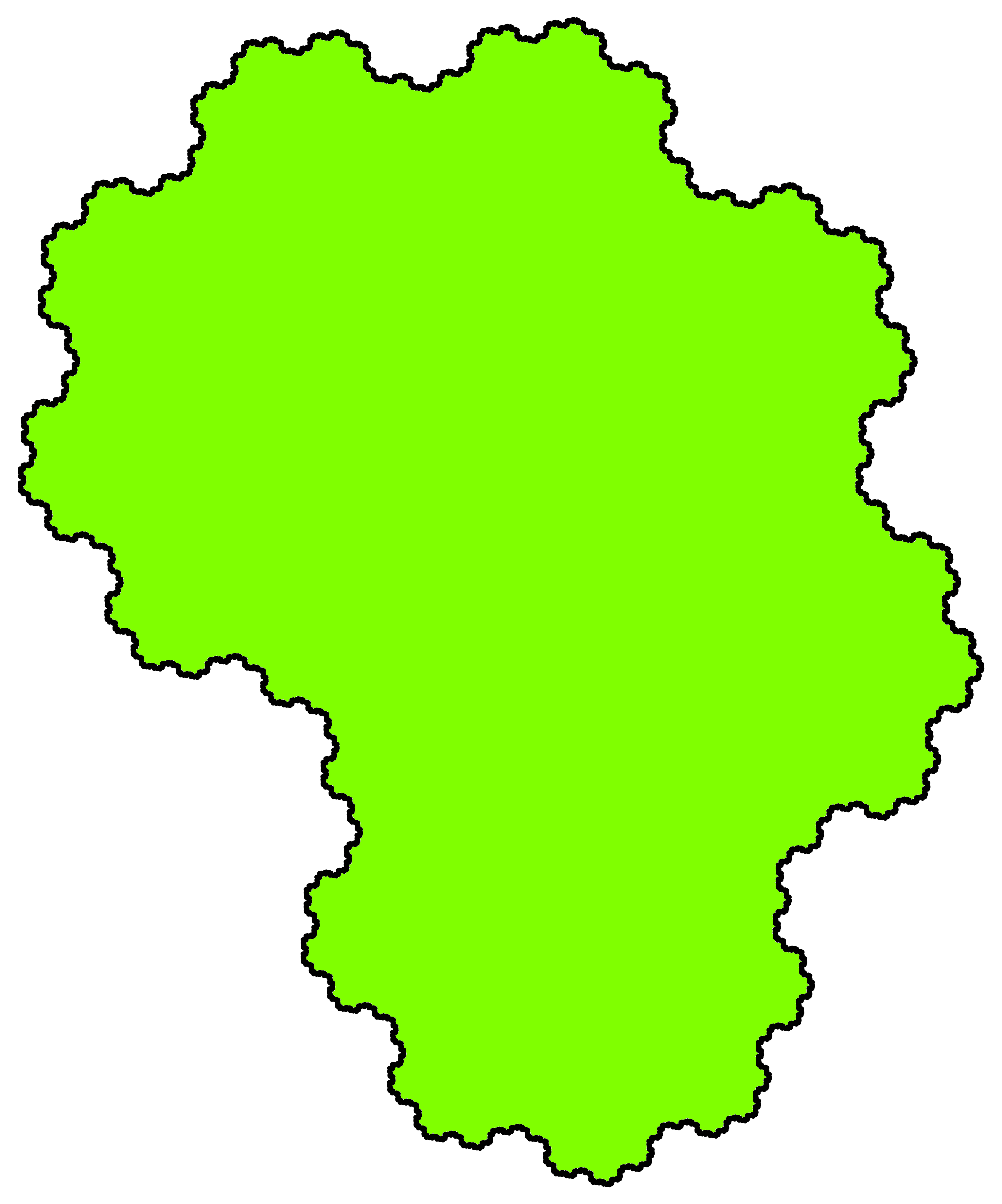
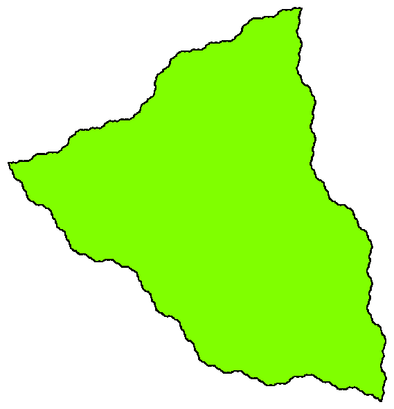
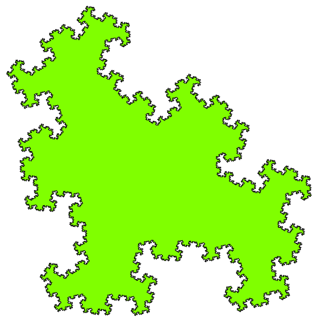
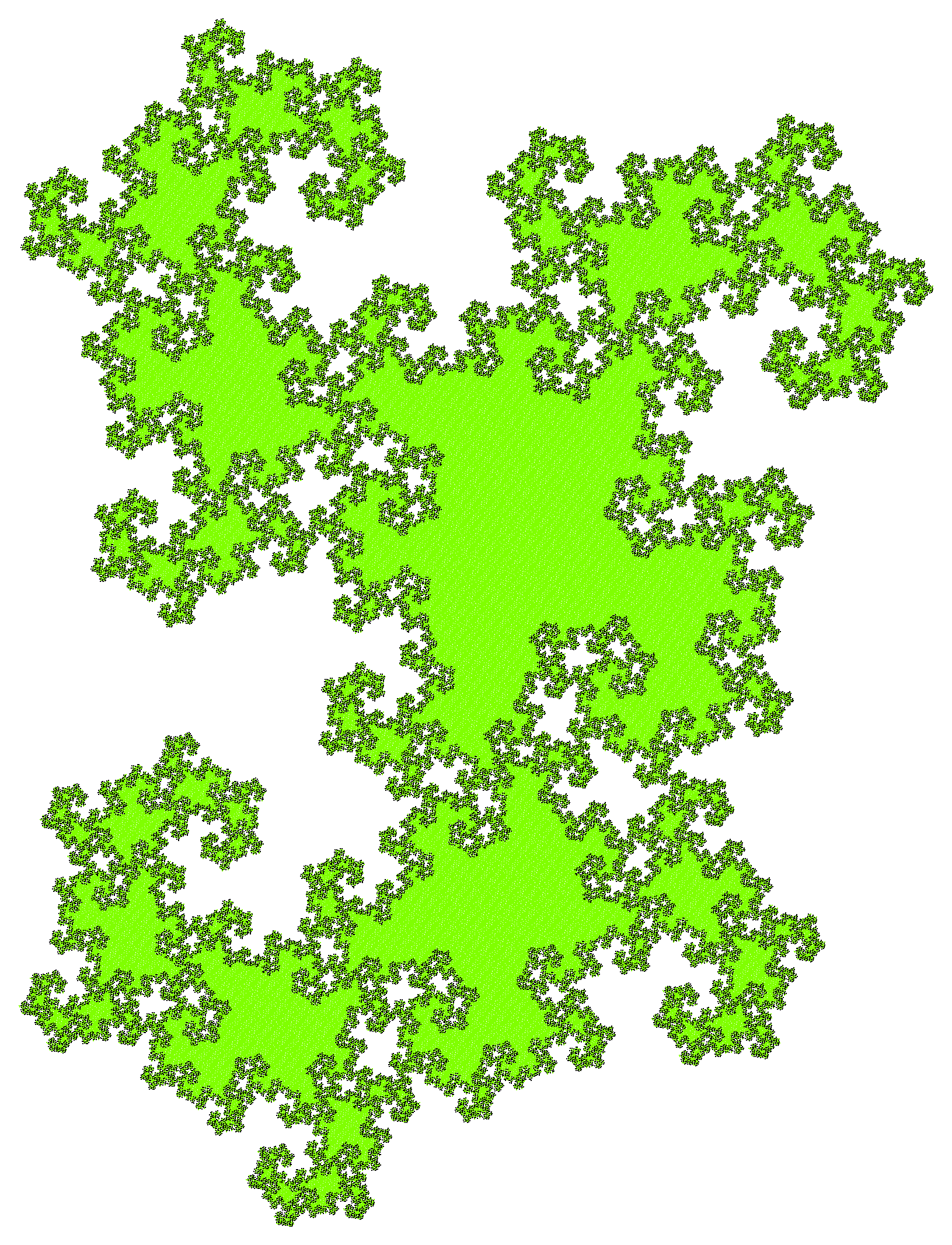
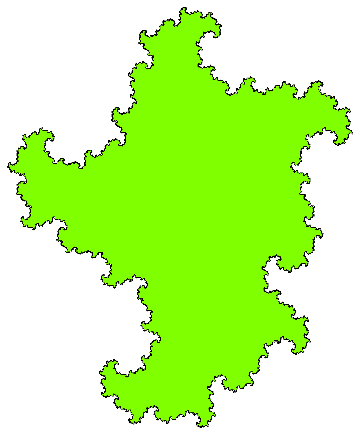
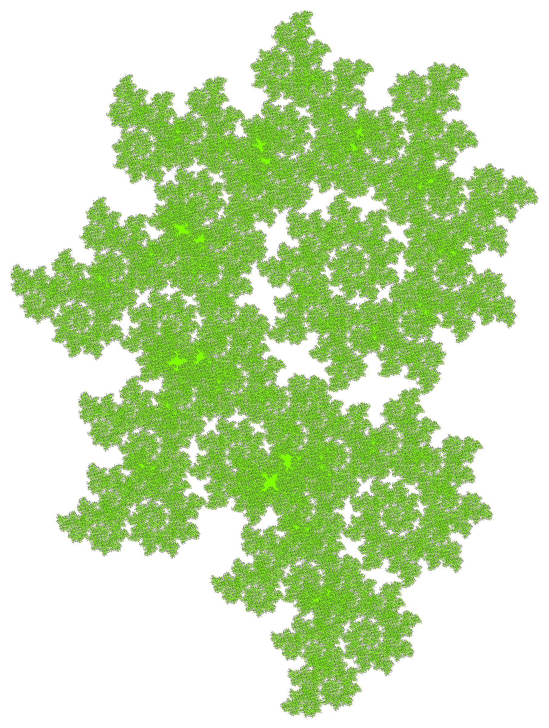
Figure 1. There are six planar tent-tiles. They all have a fractal shape.

In the present paper we introduce and study tent-tiles, i.e. geometrical objects induced by the tent map. The main idea is to consider the Galois conjugates for algebraic parameters $\alpha$ and to study the respective action of the two branches of $T_{\alpha}$. This construction is related to dual systems of algebraic iterated function systems as presented in [21]. In particular, suppose that $\alpha$ is a Pisot unit such that $\beta$ is also a Pisot unit. Let $d+1$ denote the algebraic degree of $\alpha$, ${A}_{\alpha}\in{\mathbb{R}}^{d\times d}$ be a matrix similar to ${\rm diag}\left(\lambda_{1},\ldots,\lambda_{d}\right)$, where $\lambda_{1},\ldots,\lambda_{d}$ are the Galois conjugates of $\alpha$, and

$${\Psi}_{\alpha}:{\mathbb{Q}}(\alpha)\longrightarrow{\mathbb{R}}^{d}$$

be the (uniquely determined) embedding that satisfies ${\Psi}_{\alpha}(\alpha x)={A}_{\alpha}{\Psi}_{\alpha}(x)$ for all $x\in{\mathbb{Q}}(\alpha)$. Define ${B}_{\alpha}:={A}_{\alpha}({A}_{\alpha}-{I}_{d})^{-1}\in{\mathbb{R}}^{d\times d}$, where ${I}_{d}$ denotes the $d\times d$ identity matrix. Then ${A}_{\alpha}$ and ${B}_{\alpha}$ are contractive matrices and the two functions

$$f_{L} :{\mathbb{R}}^{d}\longrightarrow{\mathbb{R}}^{d},{\bm{x}}\longmapsto{A}_{\alpha}{\bm{x}},$$

$$f_{R} :{\mathbb{R}}^{d}\longrightarrow{\mathbb{R}}^{d},{\bm{x}}\longmapsto{B}_{\alpha}({\Psi}_{\alpha}(1)-{\bm{x}})$$

induce an iterated function system in the sense of [15] (IFS for short) in the Euclidean space ${\mathbb{R}}^{d}$. The tent-tile is the invariant set induced by this IFS, that is the uniquely determined non-empty compact set $\mathcal{F}_{\alpha}$ that satisfies $\mathcal{F}_{\alpha}=f_{L}(\mathcal{F}_{\alpha})\cup f_{R}(\mathcal{F}_{\alpha})$. Up to a linear transformation, $\mathcal{F}_{\alpha}$ does not depend on the particular choice of ${A}_{\alpha}$.

A Pisot number $\alpha$ is called a special Pisot number when $\beta(\alpha)$ is also a Pisot number. Smyth showed in [26] that there exist exactly $11$ special Pisot numbers (see Table 1) where all of them but $\alpha=\alpha_{0}=2$ are algebraic units. Therefore, we only have ten cases to study. However, this allows us to explicitly investigate each of them . Interestingly, the tiles show up many different behaviours and properties. Figure 1 shows the six planar cases associated with the cubic special Pisot numbers (from left to right) $\alpha_{1}$, $\alpha_{3}$, $\alpha_{5}$, $\alpha_{-1}$, $\alpha_{-3}$, $\alpha_{-5}$. We see that tent-tiles have a fractal shape.

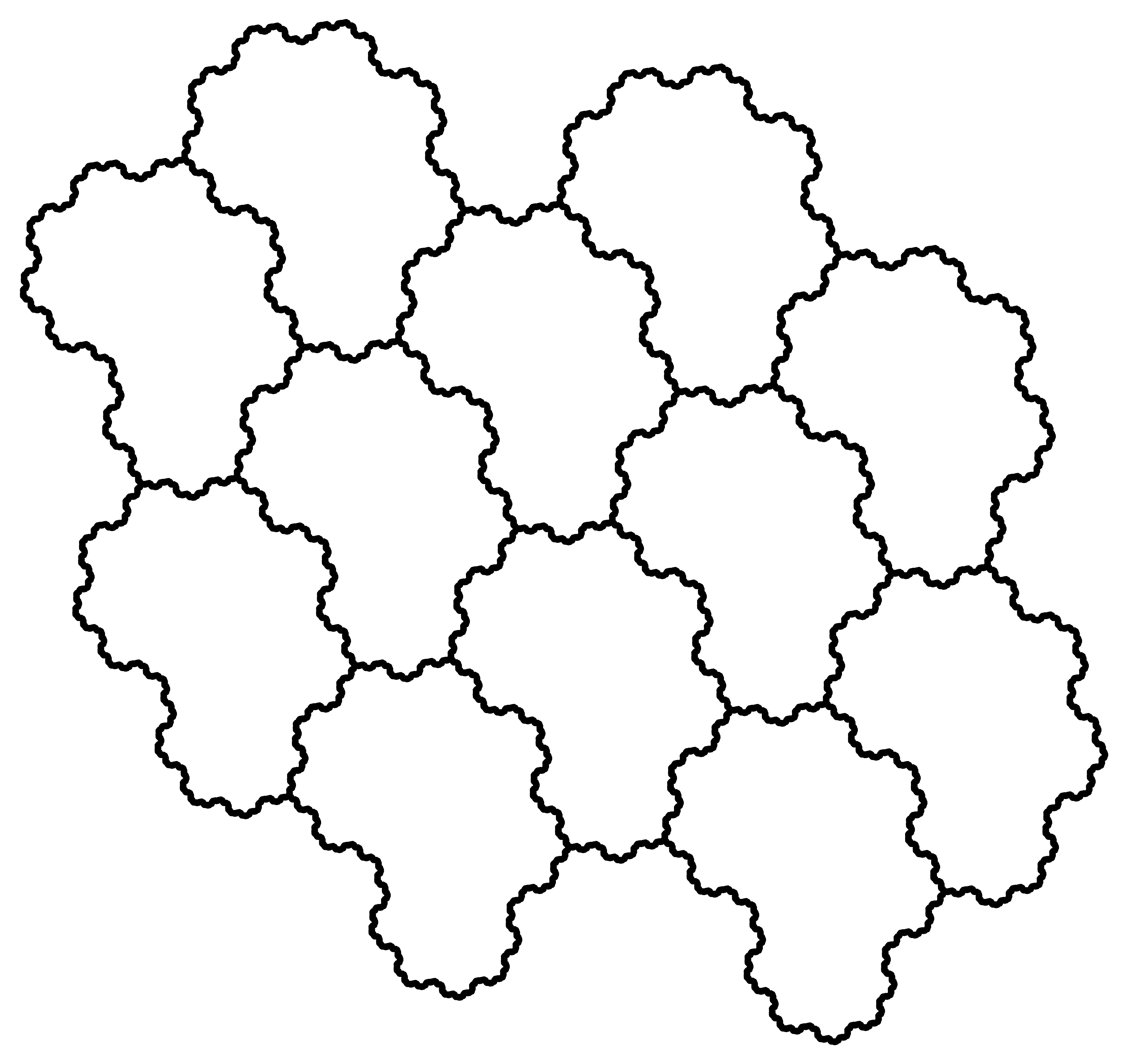
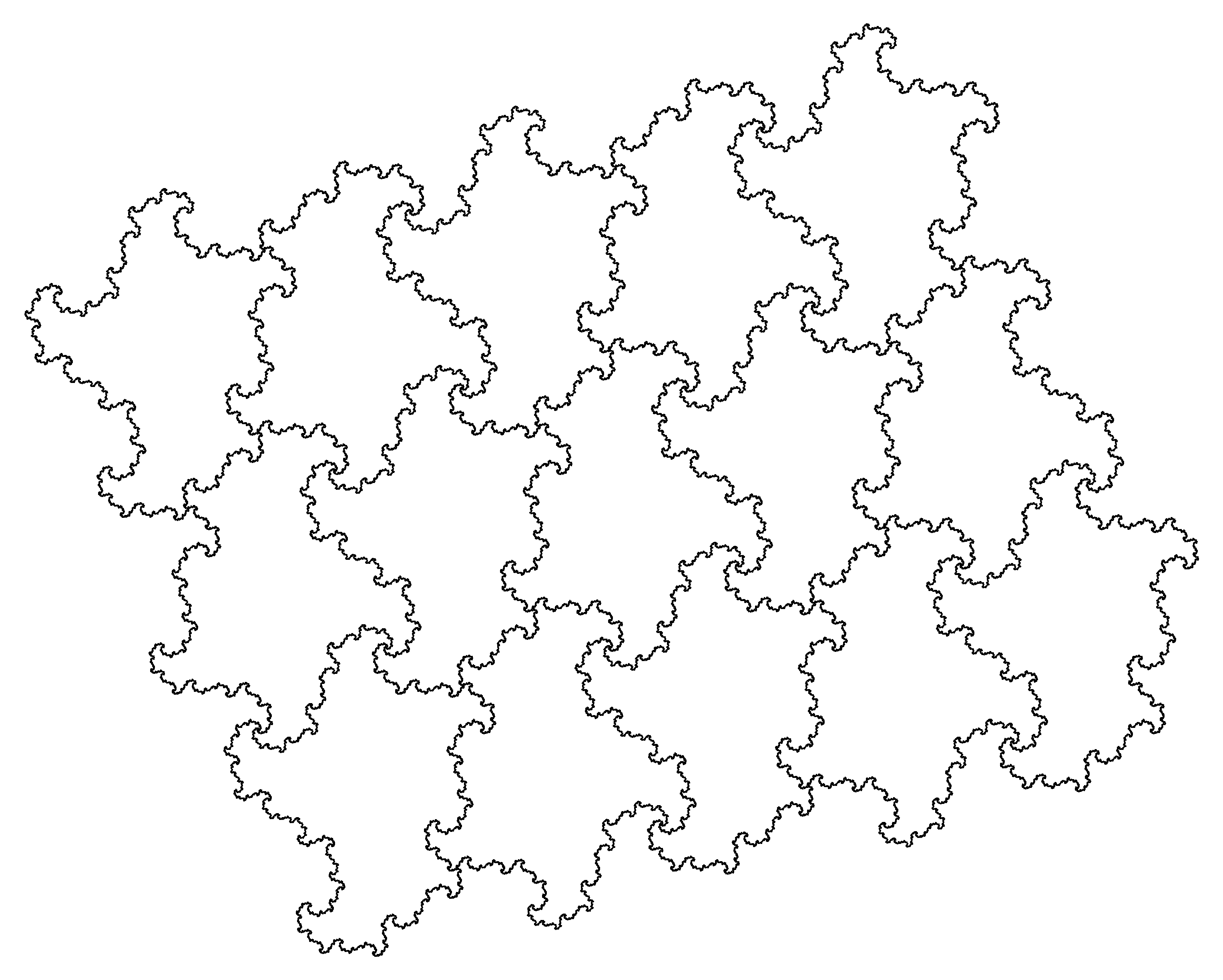
Figure 2. Two types of lattice tilings induced by tent-tiles. On the left hand side the tile itself produces the tiling. On the right hand side the tiling is generated by the tile and its reflection.

As main result we present several topological characteristics of the tent-tiles. Our first result induces that the tiles have positive Lebesgue measure.

Theorem 1.1.

Each tent-tiles is a compact sets that is the closure of its interior.

We are also interested in the Hausdorff dimension of the boundary of the tent-tiles. Here we obtain either concrete values or at least upper bounds (for the three-dimensional ones) as displayed in Table 1. Finally, we are concerned with periodic lattice tilings induced by tent-tiles. We find out that for some special Pisot numbers the tent-tile provides a periodic lattice tiling of the Euclidean space ${\mathbb{R}}^{d}$ (see the left hand side of Figure 2). For other special Pisot numbers the associated tent-tile and its reflection produce a periodic tiling (see the right hand side of Figure 2). But there are also two special Pisot numbers that do not seem to provide one of these two types of lattice tiling. The concrete results are also shown in Table 1. Summarising, although there exists only a finite number of tent-tiles, they impress by their variety. Note that IFS (and therefore tent-tiles) also give rise to aperiodic tilings [7]. We will not discuss these types of tilings in the present article.

Number	Value	Minimal polynomial	${\rm dim}_{H}(\partial\mathcal{F}_{\alpha})$	Lattice tiling
$\alpha_{-5}$	$\approx 4.0796$	$t^{3}-5t^{2}+4t-1$	$\approx 1.92089$	?
$\alpha_{-4}$	$\approx 3.62966$	$t^{4}-5t^{3}+6t^{2}-4t+1$	$\leq 2.815$	yes
$\alpha_{-3}$	$\approx 3.1479$	$t^{3}-4t^{2}+3t-1$	$\approx 1.25074$	w.r.
$\alpha_{-2}$	$\approx 2.61803$	$t^{2}-3t+1$	$0$	yes
$\alpha_{-1}$	$\approx 2.32472$	$t^{3}-3t^{2}+2t-1$	$\approx 1.70018$	w.r.
$\alpha_{0}$	$2$	$x-2$	No tent-tile
$\alpha_{1}$	$\approx 1.75488$	$t^{3}-2t^{2}+t-1$	$\approx 1.10026$	yes
$\alpha_{2}$	$\approx 1.61803$	$t^{2}-t-1$	$0$	yes
$\alpha_{3}$	$\approx 1.46557$	$t^{3}-t^{2}-1$	$\approx 1.02952$	w.r.
$\alpha_{4}$	$\approx 1.38028$	$t^{4}-t^{3}-1$	$\leq 2.74421$	w.r.
$\alpha_{5}$	$\approx 1.32472$	$t^{3}-t-1$	$\approx 1.37858$	?

Table 1. The table shows the $11$ special Pisot numbers. For each $i\in\{-5,\ldots,5\}$ we have $\beta(\alpha_{i})=\alpha_{-i}$. All but $\alpha_{0}$ are algebraic units and therefore induce tent-tiles. The penultimate column shows the Hausdorff dimension of the boundary. The last column displays whether the tent-tile induces a lattice tiling, where “w.r.” means with reflection, i.e., the lattice tiling also involves the reflected tent-tile. For the two specialy Pisot numbers marked with “$?$” we could not find any type.

As the main tool for obtaining our results we show that tent-tiles are closely related with Rauzy fractals. These fractals are induced by endomorphisms of the free monoid, so called substitutions, and are, technically speaking, the union of the invariant sets of graph directed iterated function systems (GIFS for short) as discussed, for example, in [20]. This class of fractals is named after Gerard Rauzy who studied the first such object in 1982 [22]. Rauzy’s approach has been generalised in [3, 12, 16]. Since then Rauzy fractals have been studied in innumerable researches. An overview can be obtained from more comprehensive discourses and survey articles [9, 8, 13, 24].

One more time we will see how different the particular tent-tiles behave. For our analysis we have to consider four classes of substitutions. We will see that some tent-tiles are given by the induced Rauzy fractals, other tent-tiles are related with the respective Rauzy fractals. More precisely, the tent-tiles can be obtained by unifying only particular (and sometimes also translated) elements of the invariant set list of the associated GIFS.

Actually, it is only half of the story when we speak about substitutions in context with tent-tiles. In three of the four cases mentioned above there is a much more general theory beyond, namely, dynamics induced by automorphisms of the free group. This theory is a direct extension of substitutions and also induce fractal representations which are, in fact, Rauzy fractals (with respect to certain substitutions derived from the automorphism). For a detailed discussion on this topic we refer to [10, 2]. The theory is quite complex and a proper introduction would go beyond the scope of this article. In order to keep our discourse as self-contained as possible we manage to formulate and proof all results in terms of substitutions and use only some minor results from [2] that can be easily understood without knowing the theory beyond. However, we put several remarks within the paper that contain references and links to the theory of automorphisms of the free group.

The article is organised in the following way. In Section 2 we state notations concerning special Pisot numbers and GIFS (which are generalisations of IFS) and use them to give a proper definition of the tent-tiles. We also describe what we mean by a tiling. Furthermore, we completely discuss the one-dimensional tent-tiles associated with $\alpha_{2}$ and $\alpha_{-2}$. In Section 3 we introduce the necessary theory of substitutions and Rauzy fractals and recall some important results concerning their topological properties. In Section 4 we state the exact relations between tent-tiles and Rauzy fractals induced by certain classes of substitutions. Finally, in Section 5 we use the relations that we elaborated in order to prove our main results.

2. Preliminaries

2.1. Special Pisot numbers

Let $\alpha$ be a an algebraic integer of degree $d+1$ and denote by $\gamma_{1},\ldots,\gamma_{d}$ the Galois conjugates different from $\alpha$. We say that $\alpha$ is a Pisot number if $\alpha$ is a positive real number and ${\left\lvert\gamma_{k}\right\rvert}<1$ for all $k=1,\ldots,d$. This automatically implies that $\alpha>1$.

Now, let $\beta=\beta(\alpha):=\alpha(\alpha-1)^{-1}$. Following [17] we call $\alpha$ a special Pisot number if both $\alpha$ and $\beta$ are Pisot numbers. Observe that special Pisot numbers appear pairwise. Indeed, from $\beta(\beta(\alpha)))=\alpha$ we conclude that if $\alpha$ is a special Pisot number then $\beta(\alpha)$ is a special Pisot number, too.

The most obvious special Pisot number is $\alpha=2$. In this case we have $\beta=\alpha$. Smyth [26] showed that there exist exactly ten further special Pisot numbers that are, in fact, algebraic units. Table 1 lists the special Pisot numbers and their respective minimal polynomials. An important observation is that all of these five (unordered) pairs $\{\alpha,\beta\}$ are not algebraically independent which means that there exist certain positive integers $m_{\alpha},m_{\beta}$ such that $\alpha^{m_{\alpha}}=\beta^{m_{\beta}}$. The particular dependencies are collected in Table 2.

Number	$\alpha_{1}$	$\alpha_{2}$	$\alpha_{3}$	$\alpha_{4}$	$\alpha_{5}$
$m_{i}$	$3$	$2$	$3$	$4$	$5$
Number	$\alpha_{-1}$	$\alpha_{-2}$	$\alpha_{-3}$	$\alpha_{-4}$	$\alpha_{-5}$
$m_{i}$	$2$	$1$	$1$	$1$	$1$

Table 2. The table shows the algebraic dependencies of the special Pisot numbers. For each $i\in\{-5,\ldots,5\}$ we have $\beta(\alpha_{i})=\alpha_{-i}$ and $\alpha_{i}^{m_{i}}=\alpha_{-i}^{m_{-i}}$.

2.2. Graph directed iterated function systems

Let ${\mathbb{R}}^{d}$ be the $d$-dimensional Euclidean space and denote by $\left\|\cdot\right\|$ the Euclidean norm. A contraction in ${\mathbb{R}}^{d}$ is a function $f:{\mathbb{R}}^{d}\longrightarrow{\mathbb{R}}^{d}$ such that for each $\bm{0}\not={\bm{x}}\in{\mathbb{R}}^{d}$ we have $\left\|f({\bm{x}})\right\|<\left\|{\bm{x}}\right\|$. A (finite) multigraph $G=G(V,S,E)$ is determined by a finite set of vertices $V$, a set of labels $S$, and a set of edges $E\subset V\times S\times V$, where each $(v_{1},s,v_{2})\in E$ represents an edge from $v$ to $v^{\prime}$ labelled by $s$. We denote this edge by $v\xrightarrow{s}v^{\prime}$.

By a realisation of $S$ in ${\mathbb{R}}^{d}$ we mean an operator $f$ that assigns to each label $s\in S$ a function $f_{s}:{\mathbb{R}}^{d}\longrightarrow{\mathbb{R}}^{d}$. A pair $(G,f)$ consisting of a multigraph $G$ and a realisation $f$ is called a graph-directed iterated function system (GIFS for short).

Proposition 2.1 (cf. [4, Theorem 1], [20, Theorem 1]).

Let $(G(V,S,E),f)$ be a GIFS such that for each edge $v\xrightarrow{s}v^{\prime}$ in $G$ the function $f_{s}$ is a contraction. Then there exists a uniquely determined list $\{X_{v}:v\in V\}$ of compact sets in ${\mathbb{R}}^{d}$ that satisfies the system of equations

$$X_{v}=\bigcup_{v\xrightarrow{s}v^{\prime}\in E}f_{s}(X_{v^{\prime}})\qquad(v\in V).$$ (2.1)

The list $\{X_{v}:v\in V\}$ is frequently referred to as invariant set list.

If $s$ is a contraction for all $s\in S$, then the condition on the cycles is obviously satisfied. The uniqueness of the invariant set list will play an important role in the present article.

Observe that an iterated function system (IFS) in the sense of [15] corresponds to GIFS GIFS $(G,p)$ where the graph $G$ has only one vertex. Correspondingly, the invariant set list of an IFS consists, in fact, of one invariant set only.

2.3. Definition of tent-tiles

Tent-tiles are defined as the set fixed by a graph directed construction. The set of labels is $\{L,R\}$.

The realisation depends on the particular special Pisot number $\alpha$. We fix a matrix ${A}_{\alpha}\in{\mathbb{R}}^{d\times d}$ similar to ${\rm diag}(\gamma_{1},\ldots,\gamma_{d})$ and an embedding ${\Psi}_{\alpha}:{\mathbb{Q}}(\alpha)\longrightarrow{\mathbb{R}}^{d}$ such that for all $x\in{\mathbb{Q}}(\alpha)$ we have ${\Psi}_{\alpha}(\alpha x)={A}_{\alpha}{\Psi}_{\alpha}(x)$. Denote by ${I}_{d}$ the $d\times d$ identity matrix and define ${B}_{\alpha}:={A}_{\alpha}({A}_{\alpha}-{I}_{d})^{-1}$. We clearly have that $\Psi(\beta x)={B}_{\alpha}\Psi(x)$ holds for all $x\in{\mathbb{Q}}(\alpha)$. Observe that ${A}_{\alpha}$ as well as ${B}_{\alpha}$ have a spectral radius smaller than $1$ since $\alpha$ is a special Pisot number. Furthermore, we have ${A}_{\alpha}^{-1}+{B}_{\alpha}^{-1}={I}_{d}$ which shows that

$${A}_{\alpha}{B}_{\alpha}={A}_{\alpha}+{B}_{\alpha}={B}_{\alpha}{A}_{\alpha},$$

that is the two matrices behave commutatively with respect to multiplication. We define the realisation $f$ of $\{L,R\}$ in ${\mathbb{R}}^{d}$ by

$$f_{L}:{\mathbb{R}}^{d}\longrightarrow{\mathbb{R}}^{d}, ({\bm{x}})\longmapsto{A}_{\alpha}{\bm{x}},$$

$$f_{R}:{\mathbb{R}}^{d}\longrightarrow{\mathbb{R}}^{d}, ({\bm{x}})\longmapsto{B}_{\alpha}({\Psi}_{\alpha}(1)-{\bm{x}}).$$

Note that we have

$$f_{L}^{-1}:{\mathbb{R}}^{d}\longrightarrow{\mathbb{R}}^{d}, ({\bm{x}})\longmapsto{A}_{\alpha}^{-1}{\bm{x}},$$

$$f_{R}^{-1}:{\mathbb{R}}^{d}\longrightarrow{\mathbb{R}}^{d}, ({\bm{x}})\longmapsto{\Psi}_{\alpha}(1)-{B}_{\alpha}^{-1}{\bm{x}}.$$

Observe that $f_{L}$ as well as $f_{R}$ are contractions since $\alpha$ is a special Pisot number.

Definition 2.2.

Let $\alpha$ be a special Pisot number. The tent-tile $\mathcal{F}_{\alpha}$ associated with $\alpha$ is the invariant set of the GIFS $(G_{1},f)$, where $G_{1}=G(V,\{L,R\},E)$ with $V:=\{0\}$ and $E:=\{0\xrightarrow{L}0,0\xrightarrow{L}0\}$ (see Figure 3).

Figure 3. The tent-tiles are given by the invariant set of the GIFS determined by the depicted graph.

2.4. Tilings

We consider the Euclidean space ${\mathbb{R}}^{d}$. A collection $\{Y_{i}:i\in I\}$ of compact subsets of ${\mathbb{R}}^{d}$ is a tiling of ${\mathbb{R}}^{d}$ if

1. $\bigcup_{i\in I}Y_{i}={\mathbb{R}}^{d}$ (covering property);

2. for each compact subset $Y$ of ${\mathbb{R}}^{d}$ the set $\{i\in I:Y\cap Y_{i}\not=\emptyset\}$ is finite (local finiteness);

3. there exists a positive integer $c$ such that for almost all ${\bm{x}}\in{\mathbb{R}}^{d}$ (with respect to the $d$-dimensional Lebesgue-measure) the set $\{i\in I:{\bm{x}}\in Y_{i}\}$ has exactly $c$ elements.

The integer $c$ is the so-called covering degree. If $c=1$ then we say that the tiling is a proper tiling.

2.5. One dimensional tent-tiles

We have two special Pisot units whose associated tent-tile is a subset of the real line: $\alpha_{-2}$ and $\alpha_{2}$. For these two cases the situation is quite clear and we can show the stated main results directly.

Theorem 2.3.

Let $\alpha:=\alpha_{-2}$. Then $\mathcal{F}_{\alpha}=[-\phi,0]$ is an interval, where $\phi=\frac{1+\sqrt{5}}{2}$ is the golden ratio.

Proof.

We have $\alpha=\frac{3+\sqrt{5}}{2}=\phi^{2}$ and $\beta=\phi$. Since $\alpha$ is a quadratic algebraic number we have $d=1$. Therefore, ${A}_{\alpha}={\Psi}_{\alpha}(\alpha)=\frac{3-\sqrt{5}}{2}=2-\phi$ and ${B}_{\alpha}={\Psi}_{\alpha}(\beta)=\frac{1-\sqrt{5}}{2}=1-\phi$.

Now, let $I:=[-\phi,0]$ be the stated interval and observe that $-\phi={\Psi}_{\alpha}(\beta-1)$. Due to the uniqueness of the invariant set list it suffices to show that $I$ satisfies the set equation $I=f_{L}(I)\cup f_{R}(I)$ induced by the GIFS $G_{1}$ from Definition 2.2. We leave this as an exercise to the interested reader. ∎

We immediately see that ${\mathcal{F}}_{\alpha_{-2}}$ has a positive length (i.e., positive $1$-dimensional Lebesgue measure) and the boundary of the tent-tile ${\mathcal{F}}_{\alpha_{-2}}$ consists of two points, hence ${\rm dim}_{H}(\partial{\mathcal{F}}_{\alpha_{-2}})=0$. Furthermore, the collection $\{u_{1}\phi+{\mathcal{F}}_{\alpha_{-2}}:u_{1}\in{\mathbb{Z}}\}$ obviously tiles the real line in a periodic way.

Theorem 2.4.

Let $\alpha:=\alpha_{2}$. Then $\mathcal{F}_{\alpha}=[\frac{1-\phi}{2},\frac{1}{2}]$ is an interval (and $\phi$ is the golden ratio as above).

Proof.

The proof runs analogously to that of Theorem 2.3 and is again left to the reader. ∎

As before we see that ${\mathcal{F}}_{\alpha_{2}}$ has a positive length, ${\rm dim}_{H}(\partial{\mathcal{F}}_{\alpha_{2}})=0$, and the collection $\{u_{1}\frac{\phi}{2}+{\mathcal{F}}_{\alpha_{2}}:u_{1}\in{\mathbb{Z}}\}$ is a lattice tiling.

For higher dimensional tent-tiles we need a more sophisticated strategy to prove our results.

3. Rauzy fractals

In this section we properly define Rauzy fractals and present some of their properties that we need in order to prove our results.

Let ${\mathcal{A}}=\{0,\ldots,m\}$ be an alphabet and ${\mathcal{A}}^{*}$ the set of finite words over ${\mathcal{A}}$, which includes the empty word $\varepsilon$ too. For a word $W\in{\mathcal{A}}^{*}$ and $a\in{\mathcal{A}}$ we let ${\left\lvert W\right\rvert}_{a}$ denote the number of occurrences of $a$ in $W$. Furthermore, we define ${\ell}:{\mathcal{A}}^{*}\longmapsto{\mathbb{R}}^{m}$ by

$${\ell}(W)=({\left\lvert W\right\rvert}_{0},{\left\lvert W\right\rvert}_{1},\ldots,{\left\lvert W\right\rvert}_{m})^{T}.$$

A substitution over ${\mathcal{A}}$ is a non-erasing morphism $\zeta:{\mathcal{A}}^{*}\longmapsto{\mathcal{A}}^{*}$. We say that $\zeta$ is primitive if there exists a power $k$ such that for each $a\in{\mathcal{A}}$ all entries of ${\ell}(\zeta^{k}(a))$ are strictly positive. Define the incidence matrix ${M}_{\zeta}:=({\ell}(\zeta(0)),{\ell}(\zeta(1)),\ldots,{\ell}(\zeta(m)))\in{\mathbb{R}}^{(m+1)\times(m+1)}$ and observe that for each $W\in{\mathcal{A}}^{*}$ we have ${\ell}(\zeta(W))={M}_{\zeta}\,{\ell}(W)$.

We define the prefix-graph $\Gamma_{\zeta}$ in the following way. Its set of vertices is $V=V(\Gamma_{\zeta}):=\{0,\ldots,m\}$. The labels are the proper prefixes induced by the substitution, therefore $S:={\mathcal{A}}^{*}$. There is an edge from $a$ to $b$ labelled by $U$ if $\zeta(b)=UaV$ for a word $V\in{\mathcal{A}}^{*}$, hence

$$E=E(\Gamma_{\zeta}):=\left\{a\xrightarrow{U}b:\,\exists V\in{\mathcal{A}}^{*}\text{ such that }\zeta(b)=UaV\right\}.$$

The matrix ${M}_{\zeta}$ is the adjacency matrix of $\Gamma_{\zeta}$.

If $\zeta$ is a primitive substitution then $\Gamma_{\zeta}$ is strongly connected and ${M}_{\zeta}$ is a primitive matrix. Due to the Perron-Frobenius theorem it possesses a dominant positive (real) eigenvalue that we denote by $\lambda_{0}$. Let $d+1$ be the algebraic degree of $\lambda_{0}$ and $\lambda_{1},\ldots,\lambda_{d}$ the Galois conjugates of $\lambda_{0}$. Without loss of generally we may assume that ${\left\lvert\lambda_{1}\right\rvert}\geq{\left\lvert\lambda_{2}\right\rvert}\geq\cdots\geq{\left\lvert\lambda_{d}\right\rvert}$. Clearly, $\lambda_{k}$ is also an eigenvalue of ${M}_{\zeta}$ for each $k\in\{1,\ldots,d\}$. Depending on the shape of $\bf{M}_{\zeta}$ and its eigenvalues we define several attributes for the primitive substitution $\zeta$:

• $\zeta$ is an irreducible substitution if $m=d$;

• $\zeta$ is unimodular if ${\rm det}({M}_{\zeta})=\pm 1$;

• $\zeta$ is a Pisot substitution if $\alpha$ is a Pisot number, that is ${\left\lvert\lambda_{1}\right\rvert}<1$.

For our further proceeding we exclusively concentrate on unimodular Pisot substitutions.

We now introduce a suitable decomposition of the Euclidean space ${\mathbb{R}}^{m}$ that is induced by the left eigenvectors associated with the dominant eigenvalue $\lambda_{0}$ and its conjugates. In doing so, we must take into account the fact that the set of conjugates different from $\lambda_{0}$ may contain complex conjugate pairs and, if there are further eigenvalues different from $\lambda_{0},\ldots,\lambda_{d}$, $\bf{M}_{\zeta}$ is not necessarily diagonisable.

• Let $\mathbb{K}_{e}$ be the expansive space, that is the subspace generated by the right eigenspace associated to the dominant eigenvalue $\lambda_{0}$. We clearly have that $\mathbb{K}_{e}\cong{\mathbb{R}}$.

• Let $\mathbb{K}_{c}$ be the contractive space, that is the real subspace of the space generated by the right eigenspaces associated to the Galois conjugates $\lambda_{1},\ldots,\lambda_{d}$. We have $\mathbb{K}_{c}\cong{\mathbb{R}}^{d}$.

• Let $\mathbb{K}_{s}$ be the supplementary space, that is the real subspace generated by the generalised right eigenspaces associated to the eigenvalues different from $\lambda_{0},\lambda_{1},\ldots,\lambda_{d}$. We have $\mathbb{K}_{s}\cong{\mathbb{R}}^{m-d-1}$, especially, $\mathbb{K}_{s}$ is the trivial space if $\zeta$ is irreducible.

Observe that ${\mathbb{R}}^{m}=\mathbb{K}_{e}\oplus\mathbb{K}_{c}\oplus\mathbb{K}_{s}$. For a more comprehensive discussion on this decomposition see, e.g., [8, 11, 24].

Let $\pi:{\mathbb{R}}^{m}\longrightarrow\mathbb{K}_{c}$ be a projection parallel to $\mathbb{K}_{e}$ and $\mathbb{K}_{s}$ and denote by $h$ the restriction of the action of ${M}_{\zeta}$ on $\mathbb{K}_{c}$, i.e. $\pi({M}_{\zeta}\,{\bm{y}})=h\circ\pi({\bm{y}})$ for all ${\bm{y}}\in{\mathbb{R}}^{m}$. Observe that for all ${\bm{x}}_{1},{\bm{x}}_{2}\in\mathbb{K}_{c}$ we have $\left\|h({\bm{x}}_{1})-h({\bm{x}}_{2})\right\|\leq{\left\lvert\lambda_{1}\right\rvert}\left\|{\bm{x}}_{1}-{\bm{x}}_{2}\right\|$. Especially, $h$ is a contraction since $\zeta$ is a Pisot substitution.

We now consider the realisation $g$ that assigns to each prefix $U\in S={\mathcal{A}}^{*}$ the function

$$g_{U}:\mathbb{K}_{c}\longrightarrow\mathbb{K}_{c},{\bm{x}}\longmapsto\pi\circ{\ell}(U)+h({\bm{x}}),$$

which is obviously a contraction. Therefore, the GIFS $(\Gamma_{\zeta},g)$ possesses an invariant set list that we denote by ${\mathcal{R}}_{\zeta}(0),\ldots{\mathcal{R}}_{\zeta}(m)\subset{\mathbb{R}}^{d}$. The Rauzy fractal ${\mathcal{R}}_{\zeta}$ is the union

$${\mathcal{R}}_{\zeta}={\mathcal{R}}_{\zeta}(0)\cup\ldots\cup{\mathcal{R}}_{\zeta}(m).$$ (3.1)

Proposition 3.1 ([25, Theorem 4.1]).

Let $\zeta$ be a primitive unimodular substitution over the alphabet ${\mathcal{A}}$. Then for each letter $a\in{\mathcal{A}}$ the set ${\mathcal{R}}_{\zeta}(a)$ is the closure of its interior.

The union (3.1) is not necessarily disjoint (with respect to the $d$-dimensional Lebesgue measure).

We say that two letters $a_{1}$ and $a_{2}$ have strong coincidence at prefixes if there exists an integer $k\geq 1$, a letter $b\in{\mathcal{A}}$, and words $P_{1},P_{2},S_{1},S_{2}\in{\mathcal{A}}^{*}$ such that $\zeta^{k}(a_{1})=P_{1}bS_{1}$, $\zeta^{k}(a_{2})=P_{2}bS_{2}$ and ${\ell}(P_{1})={\ell}(P_{2})$.

We say that two letters $a_{1}$ and $a_{2}$ have weak coincidence at prefixes. if there exists an integer $k\geq 1$, a letter $b\in{\mathcal{A}}$, and words $P_{1},P_{2},S_{1},S_{2}\in{\mathcal{A}}^{*}$ such that $\zeta^{k}(a_{1})=P_{1}bS_{1}$, $\zeta^{k}(a_{2})=P_{2}bS_{2}$ and $\pi\circ{\ell}(P_{1})=\pi\circ{\ell}(P_{2})$.

Definition 3.2 (Coincidence condition).

A primitive unimodular Pisot substitution $\zeta$ over ${\mathcal{A}}$ satisfies the strong coincidence condition if all letters have strong coincidence at prefixes, and $\zeta$ satisfies the weak coincidence condition if all letters have weak coincidence at prefixes.

Observe that for irreducible substitutions the notions strong coincidence and weak coincidence are equivalent. It is conjectured that all primitive irreducible unimodular Pisot substitution satisfy the strong coincidence condition (coincidence conjecture). Up to now this is only confirmed in the two-letter case [6].

The strong coincidence condition implies the union (3.1) to be (measure-theoretically) disjoint (see  [3, 11, 12, 16, 25]). We show that the weak coincidence is also sufficient.

Lemma 3.3.

Let $\zeta$ be a primitive unimodular Pisot substitution and suppose that $a_{1},a_{2}\in{\mathcal{A}}$ have weak coincidence at prefixes. Then ${\mathcal{R}}_{\zeta}(a_{1})$ and ${\mathcal{R}}_{\zeta}(a_{2})$ are measure-theoretically disjoint.

Proof.

Since $\zeta$ induces the same Rauzy fractal as $\zeta^{k}$ for all integers $k\geq 1$ we may assume, without loss of generality, that $\zeta(a_{1})=P_{1}bS_{1}$ and $\zeta(a_{2})=P_{2}bS_{2}$ with $\pi\circ{\ell}(P_{1})=\pi\circ{\ell}(P_{2})$. This implies that $(b,P_{1},a_{1})$ and $(b,P_{2},a_{2})$ are edges of the prefix-graph $\Gamma_{\zeta}$. By definition, ${\mathcal{R}}_{\zeta}(b)$ satisfies the GIFS-equation

$${\mathcal{R}}_{\zeta}(b)=\bigcup_{b\xrightarrow{U}a\in E(\Gamma_{\zeta})}g_{U}({\mathcal{R}}_{\zeta}(a)).$$

This union is measure-theoretically disjoint (see the proof of [8, Theorem 2]) and by the definition of the realisation $g$ this implies ${\mathcal{R}}_{\zeta}(a_{1})$ and ${\mathcal{R}}_{\zeta}(a_{2})$ to be measure-theoretically disjoint. ∎

Proposition 3.4 (cf [24, Proposition 3.15]).

Let $\zeta$ be an unimodular Pisot substitution such that the elements of the invariant set list $\{{\mathcal{R}}_{\zeta}(a):a\in{\mathcal{A}}\}$ have pairwise disjoint interior. Denote by $d+1$ the algebraic degree of the dominant eigenvalue. If there exist distinct letters $a_{1},\ldots,a_{d+1}\in{\mathcal{A}}$ such that

$$\forall a\in{\mathcal{A}}:\pi({\ell}(a)-{\ell}(a_{d+1}))\in\Xi_{\rm lat}:=\left\{\sum_{i=1}^{d}u_{i}\pi({\ell}(a_{i})-{\ell}(a_{d+1})):u_{1},\ldots,u_{d}\in{\mathbb{Z}}\right\}$$ (3.2)

then the collection $\left\{{\bm{\xi}}+{\mathcal{R}}_{\zeta}:{\bm{\xi}}\in\Xi_{\rm lat}\right\}$ is a tiling of the contractive space $\mathbb{K}_{c}$.

Note that Condition (3.2) is known as quotient map condition and is obviously satisfied if $\zeta$ is an irreducible substitution.

We refer to the above collection as the lattice tiling induced by $\zeta$ and we say that it possesses the tiling property if it is a proper tiling. Observe that by the so-called Pisot conjecture irreducible (unimodular Pisot) substitutions always have the tiling property. This conjecture, which is one of the most famous open problems in context with Rauzy fractals, is extensively discussed in [1]. Up to now it is confirmed for two letter substitutions [6, 14] and a class of substitutions related with beta-expansions [5].

In order to show our results concerning the topology of tent-tiles we will use some tools elaborated in [24]. We quickly state the most important facts.

At first we introduce another type of tiling induced by the Rauzy fractal ${\mathcal{R}}_{\zeta}$, more precisely, by the sets ${\mathcal{R}}_{\zeta}(0),\ldots,{\mathcal{R}}_{\zeta}(m)$. This tiling is aperiodic and it is called the self-replicated tiling. We let $\bm{u}\in{\mathbb{Q}}(\alpha)^{m+1}$ denote a left eigenvector of ${M}_{\zeta}$ with respect to the dominant eigenvalue $\alpha$ that we may assume to be strictly positive. By Perron-Frobenius theorem we may assume that all entries of $\bm{u}$ are strictly positive.

Proposition 3.5 (cf [24, Proposition 3.7]).

Let $\zeta$ be an unimodular Pisot substitution over the alphabet ${\mathcal{A}}$ and define the self-replicated translation set

$$\Xi_{\rm sr}:=\left\{(\pi({\bm{x}}),a)\in\pi({\mathbb{Z}}^{m+1})\times{\mathcal{A}}:{\bm{x}}\in{\mathbb{Z}}^{m+1},0\leq\left\langle{\bm{x}},\bm{u}\right\rangle<\left\langle{\ell}(a),\bm{u}\right\rangle\right\},$$

where $\left\langle\cdot,\cdot\right\rangle$ denotes the inner product. Then the collection $\left\{{\bm{\xi}}+{\mathcal{R}}_{\zeta}(a):({\bm{\xi}},a)\in\Xi_{{\rm sr}}\right\}$ is a tiling (the self-replicating tiling) of the contractive space $\mathbb{K}_{c}$.

Note that for irreducible substitutions the self-replicating tiling is a proper tiling if and only if the lattice tiling is proper (see [16]). An analogous statement for the reducible case (provided that Condition (3.2) is satisfied) does not seem to exist but due to the lack of counterexamples one may conjecture that such an equivalence holds for reducible substitutions, too. However, in the present article the covering degree of the self-replicating tiling is not important.

We now introduce two graphs induced by the two types of tilings, the self-replicating boundary graph $\Gamma_{\zeta}^{({\rm sr})}$ and the lattice boundary graph $\Gamma_{\zeta}^{({\rm lat})}$. In [24, Section 5.2] these graphs are discussed in a more general context. We adopted here the more compact definion given in [19].

The vertices of the two boundary graph are contained in the set

$$\mathcal{D}:=\left\{[a_{1},\pi({\bm{x}}),a_{2}]\in{\mathcal{A}}\times\pi({\mathbb{Z}}^{m+1})\times{\mathcal{A}}:\begin{array}[]{l}{\bm{x}}\in{\mathbb{Z}}^{m+1},\\ (0<\left\langle{\bm{x}},\bm{u}\right\rangle)\text{ or }(\pi({\bm{x}})=0\text{ and }a_{1}<a_{2})\end{array}\right\}.$$

The labels are elements of $\pi({\mathbb{Z}}^{m+1})\subset\mathbb{K}_{c}$.

Definition 3.6 (cf. [19, Definition 2.1]).

The self-replicating boundary graph $\Gamma_{\zeta}^{({\rm sr})}$ and the lattice boundary graph $\Gamma_{\zeta}^{({\rm lat})}$, respectively, are the largest graphs with the following properties

1. For each vertex $[a_{1},{\bm{\xi}},a_{2}]\in\mathcal{D}$ we have

   $$\left\|{\bm{\xi}}\right\|\leq\frac{2\max_{(a,U,b)\in E(\Gamma_{\zeta})}\left\|\pi\circ{\ell}(U)\right\|}{1-{\left\lvert\lambda_{1}\right\rvert}}.$$

2. There is an edge $e\xrightarrow{s}e^{\prime}$ with $e=[a_{1},{\bm{\xi}},a_{2}]$, $e^{\prime}=[b_{1},{\bm{\xi}}^{\prime},b_{2}]$ if and only if either

   • there exist $a_{1}\xrightarrow{U_{1}}b_{1},a_{2}\xrightarrow{U_{2}}b_{2}\in E(\Gamma_{\zeta})$ such that $h({\bm{\xi}}^{\prime})={\bm{\xi}}^{\prime}+\pi\circ{\ell}(U_{2})-\pi\circ{\ell}(U_{1})$ or

   • there exist $a_{1}\xrightarrow{U_{1}}b_{2},a_{2}\xrightarrow{U_{2}}b_{1}\in E(\Gamma_{\zeta})$ such that $h({\bm{\xi}}^{\prime})=-{\bm{\xi}}^{\prime}+\pi\circ{\ell}(U_{1})-\pi\circ{\ell}(U_{2})$.

   The respective label is given by

   $$s=\begin{cases}\pi\circ{\ell}(U_{1})&\text{if }\left\langle{\ell}(U_{1}),\bm{u}\right\rangle\leq\left\langle{\ell}(U_{2})+{\bm{x}},\bm{u}\right\rangle\\ \pi\circ{\ell}(U_{2})+{\bm{\xi}}&\text{otherwise}\end{cases}$$

   where ${\bm{x}}\in{\mathbb{Z}}^{m+1}$ such that $\pi({\bm{x}})={\bm{\xi}}$.

3. Each vertex belongs to an infinite walk that starts from a vertex $[a_{1},{\bm{\xi}},a_{2}]$ with $({\bm{\xi}},a_{2})\in\Xi_{sr}$ (in the case of $\Gamma_{\zeta}^{({\rm sr})}$) or ${\bm{\xi}}\in\Xi_{lat}\setminus\{\mathbf{0}\}$ (in the case of $\Gamma_{\zeta}^{({\rm lat})}$).

Observe that by [24, Proposition 5.5] both $\Gamma_{\zeta}^{({\rm lat})}$ and $\Gamma_{\zeta}^{({\rm sr})}$ are well defined and finite. In accordance with our previous way of notation we let $V(\Gamma_{\zeta}^{({\rm lat})})$ denote the set of vertices of the graph $\Gamma_{\zeta}^{({\rm lat})}$ and $E(\Gamma_{\zeta}^{({\rm lat})})$ its set of edges. Analogously, $V(\Gamma_{\zeta}^{({\rm sr})})$ and $E(\Gamma_{\zeta}^{({\rm sr})})$ are the vertices and edges, respectively, of $\Gamma_{\zeta}^{({\rm sr})}$.

The lattice boundary graph and the self-replicated boundary graph contain valuable informations concerning the tiling property and the topology of Rauzy fractals. We let $\mu_{\rm lat}$ denote the dominant eigenvalue of the incidence matrix of the lattice boundary graph $\Gamma_{\zeta}^{({\rm lat})}$. Analogously, $\mu_{\rm sr}$ is the dominant eigenvalue of the incidence matrix of the self-replicated boundary graph $\Gamma_{\zeta}^{({\rm sr})}$. At first we state that these eigenvalues allow us to verify whether the respective tilings are proper.

Proposition 3.7 (cf. [24, Theorem 4.1]).

Let $\zeta$ be a unimodular Pisot substitution. Then the self-replicating tiling is a proper tiling if and only if $\mu_{\rm sr}<\lambda_{0}$. If $\zeta$ satisfies Condition (3.2) then the lattice tiling is a proper tiling if and only if $\mu_{\rm lat}<\lambda_{0}$.

For studying the dimension of the boundary of Rauzy fractals we concentrate on the self-replicating boundary graph. This graph allows us to describe the intersections of the elements of the self-replicating tiling in terms of a GIFS. In particular, we define the realisation $g^{\prime}$ that assigns to each ${\bm{\xi}}\in\mathbb{K}_{c}$ the linear map

$$g^{\prime}_{{\bm{\xi}}}:\mathbb{K}_{c}\longrightarrow\mathbb{K}_{c},\bm{x}\longmapsto{\bm{\xi}}+h(\bm{x}),$$

which is a contraction since $h$ is a contraction. The GIFS $(\Gamma_{\zeta}^{({\rm sr})},g^{\prime})$ induces an invariant set list $\{X_{v}:v\in V(\Gamma_{\zeta}^{({\rm sr})})\}$. We have the following lemma.

Lemma 3.8 (cf. [24, Theorem 5.7]).

Let $\zeta$ be a primitive unimodular Pisot substitution over the alphabet ${\mathcal{A}}$. Then $[a_{1},{\bm{\xi}},a_{2}]\in V(\Gamma_{\zeta}^{({\rm sr})})$ if and only if $({\bm{\xi}},a_{2})\in\Xi_{\rm sr}$ and ${\mathcal{R}}_{\zeta}(a_{1})\cap({\bm{\xi}}+{\mathcal{R}}_{\zeta}(a_{2}))\not=\emptyset$. In this case we have $X_{[a_{1},{\bm{\xi}},a_{2}]}={\mathcal{R}}_{\zeta}(a_{1})\cap{\bm{\xi}}+{\mathcal{R}}_{\zeta}(a_{2})$.

The next result is our main tool in context with fractal dimensions. We first consider the box counting dimension $\dim_{B}$ as an upper bound for the Hausdorff dimension. The proposition is based on [24, Theorem 4.4] but we do not require that the self-replicating boundary graph is strongly connected. In return, we get a slightly weaker statement.

Proposition 3.9.

Let $\zeta$ be a primitive unimodular Pisot substitution over the alphabet ${\mathcal{A}}$ and suppose that $\mu_{\rm sr}<\lambda_{0}$. Then there exists an $a\in{\mathcal{A}}$ such that

$$\dim_{B}(\partial{\mathcal{R}}_{\zeta}(a))=d+\frac{\log(\lambda_{0})-\log(\mu_{\rm sr})}{\log({\left\lvert\lambda_{d}\right\rvert})}.$$

Proof.

Let $\mathcal{C}$ be the set of strongly connected components of $\Gamma_{\zeta}^{({\rm sr})}$. For each $C\in\mathcal{C}$ we denote by $\mu_{C}$ the dominant eigenvalue of the adjacency matrix of $C$. Clearly, $\mu_{\rm sr}=\max_{C\in\mathcal{C}}\mu_{C}$.

For vertices $v,v^{\prime}\in V(\Gamma_{\zeta}^{({\rm sr})})$ let ${\rm dist}(v,v^{\prime})$ be the graph distance of $v$ and $v^{\prime}$, i.e. the length of the shortest path from $v$ to $v^{\prime}$. If there is no such path then we set ${\rm dist}(v,v^{\prime}):=\infty$. For a strongly connected component $C\in\mathcal{C}$ we define ${\rm dist}(v,C)=\min\{{\rm dist}(v,v^{\prime}):v^{\prime}\text{ is a vertex of }C\}$. By observing [20, Theorem 5] and the argumentation of the proof of [24, Theorem 4.4] we see that for each $v\in V(\Gamma_{\zeta}^{({\rm sr})})$ we have

$$\dim_{B}(X_{v})=d+\frac{\log(\lambda_{0})-\max\{\log(\mu_{C}):C\in\mathcal{C},{\rm dist}(v,C)<\infty\}}{\log({\left\lvert\lambda_{d}\right\rvert})}.$$

Finally, observe that Lemma 3.8 implies that for each $a\in{\mathcal{A}}$ we have

$$\partial{{\mathcal{R}}_{\zeta}(a)}=\bigcup_{\begin{subarray}{c}[a_{1},{\bm{\xi}},a_{2}]\in V(\Gamma_{\zeta}^{({\rm sr})})\\ a_{1}=a\vee({\bm{\xi}}=\bm{0}\wedge a_{2}=a)\end{subarray}}X_{[a_{1},{\bm{\xi}},a_{2}]}$$

and, hence,

$$\dim_{B}(\partial{\mathcal{R}}_{\zeta}(a))=\max\{\dim_{B}(X_{[a_{1},{\bm{\xi}},a_{2}]}):[a_{1},{\bm{\xi}},a_{2}]\in V(\Gamma_{\zeta}^{({\rm sr})}),a_{1}=a\vee({\bm{\xi}}=\bm{0}\wedge a_{2}=a)\}.$$

From this the statement of the proposition follows immediately. ∎

Concerning the Hausdorff dimension we obtain the following corollary.

Corollary 3.10.

Let $\zeta$ be a primitive unimodular Pisot substitution over the alphabet ${\mathcal{A}}$ and suppose that $\mu_{\rm sr}<\lambda_{0}$. Then there exists an $a\in{\mathcal{A}}$ such that

$$\dim_{H}(\partial{\mathcal{R}}_{\zeta}(a))\leq d+\frac{\log(\lambda_{0})-\log(\mu_{\rm sr})}{\log({\left\lvert\lambda_{d}\right\rvert})}.$$

If ${\left\lvert\lambda_{1}\right\rvert}={\left\lvert\lambda_{d}\right\rvert}$ then equality holds.

4. Relations between tent-tiles and Rauzy fractals

In the present section we show the exact relation between tent-tiles and four classes of substitutions. For an integer $p\geq 3$ let $\zeta_{p}$ denote the substitution

$$\zeta_{p}:0\mapsto 10,1\mapsto 2,\ldots,(p-2)\mapsto(p-1),(p-1)\mapsto(p-1)0.$$ (4.1)

over the alphabet ${\mathcal{A}}=\{0,\ldots,p-1\}$. The prefix graph $\Gamma_{\zeta_{p}}$ is sketched in Figure 4.

Figure 4. Prefix graph of the substitution $\zeta_{p}$.

Note that the substitution $\zeta_{p}$ satisfies the strong coincidence condition. Indeed, it is easy to see that $\zeta_{p}^{p-1}(a)$ starts with the letter $p-1$ for each letter $a\in{\mathcal{A}}$.

Theorem 4.1.

Let $\alpha$ be a special Pisot unit such that $\alpha^{p}=\beta^{2}$ holds for an integer $p\geq 3$. Then $\zeta_{p}$ (as defined in (4.1)) is a primitive unimodular Pisot substitution with dominant root $\alpha$ and there exists a linear isomorphism $\Phi:{\mathbb{R}}^{d}\longmapsto\mathbb{K}_{c}$ such that for each $k\in{\mathcal{A}}$ we have ${\mathcal{R}}_{\zeta^{\prime}_{p}}(k)=\Phi(X_{k})$ with

$$X_{k}=\begin{cases}f_{L}^{k}\circ f_{R}(\mathcal{F}_{\alpha})&\text{if }k\in\{0,\ldots,p-2\},\\ f_{L}^{p-1}(\mathcal{F}_{\alpha})&\text{if }k=p-1.\end{cases}$$

Proof.

The substitution $\zeta_{p}$ is obviously primitive. The incidence matrix of $\zeta_{p}$ is given by

$${M}_{\zeta_{p}}=\left(\begin{array}[]{ccccc}1&0&\cdots&0&1\\ 1&0&\cdots&0&0\\ 0&1&\ddots&\vdots&\vdots\\ \vdots&\ddots&\ddots&0&0\\ 0&\cdots&0&1&1\end{array}\right).$$

One easily verifies that the characteristic polynomial is given by $t^{p}-2t^{p-1}+t^{p-2}-1$ and that the dominant root of this polynomial is $\alpha$. Therefore, the substitution is a unimodular Pisot substitution and induces a Rauzy fractal.

The strategy of the proof is the following: for a certain linear transformation $\Phi$ we show that the set list $\{\Phi(X_{0}),\ldots,\Phi(X_{p}-1)\}$ satisfies the system of set equations (2.1) induced by the GIFS $(\Gamma_{\zeta_{p}},g)$. Then the assertion of the theorem follows directly from the uniqueness if the invariant set list in Proposition 2.1.

Let $\bm{u}:=(\beta,\alpha,\alpha^{2},\ldots,\alpha^{p-1})$. We claim that $\bm{u}$ is a left eigenvector of ${M}_{\zeta_{p}}$ with respect to $\alpha$. Indeed, $\bm{u}\,{M}_{\zeta}=(\beta+\alpha,\alpha^{2},\alpha^{3},\ldots,\alpha^{p-1},\beta+\alpha^{p-1})$ and by the definition of $\beta=\beta(\alpha)$ we have $\beta+\alpha=\alpha\beta$ and $\beta+\alpha^{p-1}=\alpha^{p}\beta^{-1}+\alpha^{p}\alpha^{-1}=\alpha^{p}$, hence $\bm{u}\,{M}_{\zeta_{p}}=\alpha\,\bm{u}$. Let

$${P}:=\left(\begin{array}[]{ccccc}-{\Psi}_{\alpha}(\beta)&-{\Psi}_{\alpha}(\alpha)&-{\Psi}_{\alpha}(\alpha^{2})&\cdots&-{\Psi}_{\alpha}(\alpha^{p-1})\end{array}\right)\in{\mathbb{R}}^{d\times p},$$

where ${\Psi}_{\alpha}:{\mathbb{Q}}(\alpha)\longrightarrow{\mathbb{R}}^{d}$ is the embedding as defined in Subsection 2.3. We let $\Phi$ be the (uniquely determined) linear map that satisfies $\pi({\bm{y}})=\Phi\left({P}\,{\bm{y}}\right)$ for all ${\bm{y}}\in{\mathbb{R}}^{p}$. Since ${P}\,{M}_{\zeta_{p}}={A}_{\alpha}\,{P}$ we immediately see that $h\circ\Phi({\bm{x}})=\Phi({A}_{\alpha}\,{\bm{x}})$ for all ${\bm{x}}\in{\mathbb{R}}^{d}$. Then, for each prefix $U\in{\mathcal{A}}^{*}$ we have

$$g_{U}\circ\Phi:{\mathbb{R}}^{d}\longmapsto\mathbb{K}_{c},{\bm{x}}\longmapsto\pi\circ{\ell}(U)+h\circ\Phi({\bm{x}})=\Phi\left({P}\,{\ell}(U)+{A}_{\alpha}{\bm{x}}\right).$$

Concretely, for the appearing pairs of labels we easily obtain

$$\begin{array}[]{rll}g_{\varepsilon}\circ\Phi\left({\bm{x}}\right)&=\Phi\left({P}\,{\ell}(\varepsilon)+{A}_{\alpha}{\bm{x}}\right)&=\Phi\circ f_{L}({\bm{x}}),\\ g_{1}\circ\Phi\left({\bm{x}}\right)&=\Phi({P}\,{\ell}(1)+{A}_{\alpha}{\bm{x}})=\Phi({\Psi}_{\alpha}(-\alpha)+{B}_{\alpha}\,{B}_{\alpha}^{-1}\,{A}_{\alpha}\,{\bm{x}})\\ &=\Phi\left({\Psi}_{\alpha}(\beta)-{\Psi}_{\alpha}(\beta\alpha)+{B}_{\alpha}\,{A}_{\alpha}\,{B}_{\alpha}^{-1}\,{\bm{x}}\right)&=\Phi\circ f_{R}\circ f_{L}\circ f_{R}^{-1}({\bm{x}}),\\ g_{p-1}\circ\Phi\left({\bm{x}}\right)&=\Phi\left({\Psi}_{\alpha}(-\alpha^{1-p})+{A}_{\alpha}\right)\\ &=\Phi\left({\Psi}_{\alpha}(\beta^{2}(\beta^{-1}-1))+{B}_{\alpha}^{2}\,{A}_{\alpha}^{1-p}\,{\bm{x}}\right)\\ &=\Phi\left({\Psi}_{\alpha}(\beta)-{\Psi}_{\alpha}(\beta^{2})+{B}_{\alpha}^{2}\,{A}_{\alpha}^{1-p}\,{\bm{x}}\right)&=\Phi\circ f_{R}^{2}\circ f_{L}^{1-p}({\bm{x}}).\end{array}$$

We are now in the position to verify that the system of set equations is satisfied. Observe that $f_{L}(\mathcal{F}_{\alpha})\cup f_{R}(\mathcal{F}_{\alpha})=\mathcal{F}_{\alpha}$. For each $k\in\{1,\ldots,p-2\}$ we immediately see that $\Phi(X_{k})=\Phi\circ f_{L}^{k}\circ f_{R}(\mathcal{F}_{\alpha})=g_{\varepsilon}\circ\Phi\circ f_{L}^{k-1}\circ f_{R}(\mathcal{F}_{\alpha})=g_{\varepsilon}\circ\Phi(X_{k-1})$. Furthermore, we have

$$\Phi\left(X_{0}\right)=\Phi\circ f_{R}(\mathcal{F}_{\alpha})= \Phi\left(f_{R}\circ f_{L}(\mathcal{F}_{\alpha})\cup f_{R}^{2}(\mathcal{F}_{\alpha})\right)$$

$$= \Phi\circ f_{R}\circ f_{L}\circ f_{R}^{-1}\circ f_{R}(\mathcal{F}_{\alpha})\cup\Phi\circ f_{R}^{2}\circ f_{L}^{1-p}\circ f_{L}^{p-1}(\mathcal{F}_{\alpha})$$

$$= g_{1}\circ\Phi\left(X_{0}\right)\cup g_{p-1}\circ\Phi\left(X_{p-1}\right).$$

Finally, $\Phi\left(X_{p-1}\right)=\Phi\circ f_{L}^{p-1}(\mathcal{F}_{\alpha})=\Phi\circ f_{L}^{p-1}\circ f_{L}(\mathcal{F}_{\alpha})\cup\Phi\circ f_{L}^{p-1}\circ f_{R}(\mathcal{F}_{\alpha})=g_{\varepsilon}\circ\Phi\left(X_{p-1}\right)\cup g_{\varepsilon}\circ\Phi\left(X_{p-2}\right)$. ∎

Observe that this result asserts that five of the tent-tiles are Rauzy fractals.

Corollary 4.2.

The tent-tiles ${\mathcal{F}}_{\alpha_{1}}$, ${\mathcal{F}}_{\alpha_{2}}$, ${\mathcal{F}}_{\alpha_{3}}$, ${\mathcal{F}}_{\alpha_{4}}$ and ${\mathcal{F}}_{\alpha_{5}}$ are (up to a linear isomorphism) given by the Rauzy fractals induced by $\zeta_{3}$, $\zeta_{4}$, $\zeta_{6}$, $\zeta_{8}$ and $\zeta_{10}$, respectively.

Proof.

Table 2 shows that the special Pisot units $\alpha_{1}$, $\alpha_{2}$, $\alpha_{3}$, $\alpha_{4}$ and $\alpha_{5}$ satisfy the conditions of Theorem 4.1 (for respective integers $p$). The identity $\mathcal{F}_{\alpha}=X_{0}\cup\cdots\cup X_{p-1}$ is easy to see. ∎

We introduce three further families of substitutions and show that they are intimately related with tent-tiles. The proofs of the respective theorems run with the strategy used in the proof of Theorem 4.1. Observe that these families of substitutions are induced by automorphisms of the free group. These automorphisms are stated explicitly in respective remarks at the end of the each proof.

At first we consider the substitution $\theta_{q}$ over the alphabet ${\mathcal{A}}=\{0,\ldots,q-1,2q-1\}$ defined by

$$\begin{array}[]{lrcl@{\qquad}rcl}\theta_{q}:&0&\mapsto&1,&q&\mapsto&(q+1),\\ &1&\mapsto&2&(q+1),&\mapsto&(q+2),\\ &&\vdots&&&\vdots&\\ &(q-2)&\mapsto&(q-1),&(2q-2)&\mapsto&(2q-1),\\ &(q-1)&\mapsto&q(q-1),&(2q-1)&\mapsto&(2q-1)0.\end{array}$$ (4.2)

Figure 5. Prefix graph of the substitution $\theta_{q}$.

Its prefix graph $\Gamma_{\theta_{q}}$ is depicted in Figure 5. Note that $\theta_{q}^{2q}(k)$ starts with the letter $2q-1$ for each $k\in{\mathcal{A}}$. Therefore, $\zeta_{q}$ satisfies the strong coincidence condition.

Theorem 4.3.

Let $\alpha$ be a special Pisot unit such that $\alpha^{q}=\beta$ holds for an integer $q\geq 2$ and define for each $k\in{\mathcal{A}}:=\{0,\ldots,2q-1\}$ the set $X_{k}$ by

$$X_{k}=\begin{cases}{\Psi}_{\alpha}(\alpha^{k})-f_{L}^{k}\circ f_{R}(\mathcal{F}_{\alpha})&\text{if }k\in\{0,\ldots,q-2\},\\ {\Psi}_{\alpha}(\alpha^{q-1})-f_{L}^{q-1}(\mathcal{F}_{\alpha})&\text{if }k=q-1\\ f_{L}^{k-q}\circ f_{R}(\mathcal{F}_{\alpha})&\text{if }k\in\{q,\ldots,2q-2\},\\ f_{L}^{q-1}(\mathcal{F}_{\alpha})&\text{if }k=2q-1.\end{cases}$$

Then $\theta_{q}$ (as defined in (4.2)) is a primitive unimodular Pisot substitution with dominant root $\alpha$ and there exists a linear isomorphism $\Phi:{\mathbb{R}}^{d}\longmapsto\mathbb{K}_{c}$ such that ${\mathcal{R}}_{\theta_{q}}(k)=\Phi(X_{k})$ holds for each $k\in{\mathcal{A}}$.

Proof.

The substitution $\theta_{q}$ is obviously primitive. Its incidence matrix is given by the block matrix

$${M}_{\theta_{q}}=\left(\begin{array}[]{cc}{M}^{+}_{q}&{M}^{-}_{q}\\ {M}^{-}_{q}&{M}^{+}_{q}\end{array}\right).$$

where

$${M}^{+}_{{q}}=\left(\begin{array}[]{ccccc}0&\cdots&\cdots&0&0\\ 1&\ddots&&\vdots&\vdots\\ 0&\ddots&\ddots&\vdots&\vdots\\ \vdots&\ddots&\ddots&0&0\\ 0&\cdots&0&1&1\end{array}\right)\in{\mathbb{R}}^{q\times q}\text{ and }{M}^{-}_{{q}}=\left(\begin{array}[]{cccc}0&\cdots&0&1\\ \vdots&&\vdots&0\\ \vdots&&\vdots&\vdots\\ 0&\cdots&0&0\end{array}\right)\in{\mathbb{R}}^{q\times q}.$$ (4.3)

By observing the proof of [2, Proposition 4.9] we see that the dominant eigenvalue of ${M}_{\theta_{q}}$ is given by the dominant eigenvalue of ${M}_{q}^{+}+{M}^{-}_{q}$ which can easily seen to be the dominant root of $t^{q}-t^{q-1}-1$. From this we conclude that this root must coincide with $\alpha$.

Let $\bm{u}=(1,\alpha,\ldots,\alpha^{q-1})$ and observe that $(\bm{u},\bm{u})$ is a left eigenvector of ${M}_{\theta_{q}}$ with respect to $\alpha$. Let

$${P}:=\left(-{\Psi}_{\alpha}(1)\,-{\Psi}_{\alpha}(\alpha)\,\ldots\,-{\Psi}_{\alpha}(\alpha^{q-1})\,-{\Psi}_{\alpha}(1)\,-{\Psi}_{\alpha}(\alpha)\,\ldots\,-{\Psi}_{\alpha}(\alpha^{q-1})\right)\in{\mathbb{R}}^{d\times 2q}$$

and define $\Phi:{\mathbb{R}}^{d}\longmapsto\mathbb{K}_{c}$ such that $\pi({\bm{y}})=\Phi\left({P}\,{\bm{y}}\right)$ for all ${\bm{y}}\in{\mathbb{R}}^{p}$. We have $h\circ\Phi({\bm{x}})=\Phi({A}_{\alpha}\,{\bm{x}})$ for all ${\bm{x}}\in{\mathbb{R}}^{d}$.

The prefixes that occur in the prefix graph $\Gamma_{\theta_{q}}$ (see Figure 5) are $\varepsilon,q,2q-1$. By considering the realisation $g$ we obtain for each ${\bm{x}}\in{\mathbb{R}}^{d}$

$$\begin{array}[]{rll}g_{\varepsilon}\circ\Phi\left({\bm{x}}\right)&=\Phi\left(P\,{\ell}(\varepsilon)+{A}_{\alpha}\,{\bm{x}}\right)=\Phi\left({A}_{\alpha}\,{\bm{x}}\right)&=\Phi\circ f_{L}({\bm{x}}),\\ g_{q}\circ\Phi\left({\bm{x}}\right)&=\Phi\left(P\,{\ell}(q)+{A}_{\alpha}\,{\bm{x}}\right)=\Phi\left(-{\Psi}_{\alpha}(1)+{A}_{\alpha}\,{\bm{x}}\right)&=\Phi\left(-{\Psi}_{\alpha}(1)+f_{L}({\bm{x}})\right),\\ g_{2q-1}\circ\Phi\left({\bm{x}}\right)&=\Phi\left(-{\Psi}_{\alpha}(\alpha^{q-1})+{B}_{\alpha}\,{A}_{\alpha}^{1-q}\,{\bm{x}}\right)\\ &=\Phi\left({\Psi}_{\alpha}(1)-{\Psi}_{\alpha}(\alpha^{q})+{B}_{\alpha}\,{A}_{\alpha}^{1-q}\,{\bm{x}}\right)&=\Phi\left({\Psi}_{\alpha}(1)-f_{R}\circ f_{L}^{1-q}({\bm{x}})\right).\end{array}$$

We proceed as in Theorem 4.1 and show that the set list $\{\Phi(X_{k}):k\in{\mathcal{A}}\}$ satisfies the system set equations (2.1) induces by the GIFS $(\Gamma_{\theta^{\prime}_{q}},g)$.

For $k=0$ we easily calculate

$$\Phi\left(X_{0}\right)= \Phi\left({\Psi}_{\alpha}(1)-f_{R}(\mathcal{F}_{\alpha})\right)=\Phi\left({\Psi}_{\alpha}(1)-f_{R}\circ f_{L}^{1-q}\circ f_{L}^{q-1}(\mathcal{F}_{\alpha})\right)=g_{2q-1}\circ\Phi\left(X_{2q-1}\right).$$

For $k\in\{1,\ldots,q-2\}$ we have

$$\Phi\left(X_{k}\right) =\Phi\left({\Psi}_{\alpha}(\alpha^{k})-f_{L}^{k}\circ f_{R}(\mathcal{F}_{\alpha})\right)=\Phi\left({A}_{\alpha}({\Psi}_{\alpha}(\alpha^{k-1}))-f_{L}\circ f_{L}^{k-1}\circ f_{R}(\mathcal{F}_{\alpha})\right)$$

$$=\Phi\circ f_{L}\left({\Psi}_{\alpha}(\alpha^{k-1})-f_{L}^{k-1}\circ f_{R}(\mathcal{F}_{\alpha})\right)=g_{\varepsilon}\circ\Phi\left(X_{k-1}\right).$$

For $k=q-1$ we obtain

$$\Phi\left(X_{q-1}\right)= \Phi\left(\Psi_{\alpha}(\alpha^{q-1})-f_{L}^{q-1}(\mathcal{F}_{\alpha})\right)$$

$$= \Phi\big{(}\Psi_{\alpha}(\alpha^{q-1})-f_{L}^{q-1}\circ f_{R}(\mathcal{F}_{\alpha})\big{)}\cup\Phi\big{(}\Psi_{\alpha}(\alpha^{q-1})-f_{L}^{q}(\mathcal{F}_{\alpha})\big{)}$$

$$= \Phi\left(\Psi_{\alpha}(\alpha^{q-1})-f_{L}^{q-1}\circ f_{R}(\mathcal{F}_{\alpha})\right)\cup\Phi\big{(}-\Psi_{\alpha}(1)+\Psi_{\alpha}(\alpha^{q})-f_{L}^{q}(\mathcal{F}_{\alpha})\big{)}$$

$$= \Phi\circ f_{L}\big{(}\Psi_{\alpha}(\alpha^{q-2})-f_{L}^{q-2}\circ f_{R}(\mathcal{F}_{\alpha})\big{)}\cup\Phi\left(-\Psi_{\alpha}(1)+f_{L}\big{(}\Psi_{\alpha}(\alpha^{q-1})-f_{L}^{q-1}(\mathcal{F}_{\alpha})\big{)}\right)$$

$$= g_{\varepsilon}\circ\Phi(X_{q-2})\cup g_{q}\circ\Phi(X_{q-1}).$$

For $k=q$ we see that

$$\Phi\left(X_{q}\right)= \Phi\circ f_{R}(\mathcal{F}_{\alpha})=f_{L}^{q}\,\big{(}{\Psi}_{\alpha}(1)-\mathcal{F}_{\alpha}\big{)}$$

$$= \Phi\circ f_{L}\big{(}{\Psi}_{\alpha}(\alpha^{q-1})-f_{L}^{q-1}(\mathcal{F}_{\alpha})\big{)}=g_{\varepsilon}\circ\Phi(X_{q-1}).$$

Now we let $k\in\{q+1,\ldots,2q-1\}$. Here trivial computations yield

$$\Phi\left(X_{k}\right)=\Phi\circ f_{L}^{k-q}\circ f_{R}(\mathcal{F}_{\alpha})=\Phi\circ f_{L}\circ f_{L}^{k-q-1}\circ f_{R}(\mathcal{F}_{\alpha})=g_{\varepsilon}\circ\Phi(X_{k-1}).$$

Finally, for $k=2q-1$ we have

$$\Phi\left(X_{2q-1}\right)= \Phi\circ f_{L}^{q-1}(\mathcal{F}_{\alpha})=\Phi\circ f_{L}^{q-1}\circ f_{R}(\mathcal{F}_{\alpha})\cup\Phi\circ f_{L}^{q}(\mathcal{F}_{\alpha})$$

$$= g_{\varepsilon}\circ\Phi(X_{2q-2})\cup g_{\varepsilon}\circ\Phi(X_{2q-1}).$$

∎

The following observation can be obtained immediately from the theorem.

Corollary 4.4.

Let $\alpha$ be a special Pisot unit such that $\alpha^{q}=\beta$ holds for an integer $q\geq 2$. Then $\mathcal{F}_{\alpha}$ coincides with ${\mathcal{R}}_{\theta_{q}}(q)\cup\cdots\cup{\mathcal{R}}_{\theta_{q}}(2q-1)$ up to a linear isomorphism.

Remark 4.5.

Observe that the substitution $\theta_{q}$ is induced by an automorphism of the free group. In particular, $\theta_{q}$ is the (non-orientable) double substitution (in the sense of [2, Definition 3.1]) of the automorphism $\varphi_{q}$ of the free group genreated by $\{0,\ldots,q-1\}$ defined by

$$\varphi_{q}:0\mapsto 1,1\mapsto 2,\ldots,(q-2)\mapsto(q-1),(q-1)\mapsto(q-1)1^{-1}.$$

The case $\varphi_{5}$ is discussed in [2, Example 5.4] and we find our tent-tile ${\mathcal{F}}_{\alpha_{5}}$ in the respective figure.

Lets turn to the next family of substitutions that we denote by $\theta^{\prime}_{q}$ with $q$ a positive integer. The exact definition depends on whether $q$ is odd or even.

If $$q\equiv 1\,({\rm mod\,}2) \theta^{\prime}_{q} {\mathcal{A}}=\{0,\ldots,2q-1\}$$ then is defined over the alphabet by

$$\begin{array}[]{cl@{\,\mapsto\,}lcl@{\,\mapsto\,}ll@{\,\mapsto\,}l}\theta^{\prime}_{q}:&0&(q+1),&\ldots,&(q-2)&(2q-1),&(q-1)&0(2q-1)\\ &q&1,&\ldots,&(2q-2)&(q-1),&(2q-1)&(q-1)q.\end{array}$$ (4.4a)

For $$q\equiv 0\,({\rm mod\,}2) \theta^{\prime}_{q} {\mathcal{A}}=\{0,\ldots,q-1\}$$ the substitution is defined over the alphabet by

$$\theta^{\prime}_{q}:0\mapsto 2,1\mapsto 3,\ldots,(q-3)\mapsto(q-1),(q-2)\mapsto 0(q-1),(q-1)\mapsto 0(q-1)1.$$ (4.4b)

For the prefix graph see Figure 6.

Figure 6. Prefix graph of the substitution $\theta^{\prime}_{q}$ for $q$ odd (left) and $q$ even (right).

Theorem 4.6.

Let $\alpha$ be a special Pisot unit such that $\alpha=\beta^{q}$ holds for an integer $q\geq 3$. Then $\theta^{\prime}_{q}$ (as defined in (4.4a) and (4.4b), respectively) is a primitive unimodular Pisot substitution with dominant root $\beta$ and there exists a linear isomorphism $\Phi:{\mathbb{R}}^{d}\longmapsto\mathbb{K}_{c}$ such that for each $k\in{\mathcal{A}}$ we have ${\mathcal{R}}_{\theta^{\prime}_{q}}(k)=\Phi(X_{k})$ with

$$X_{k}=\begin{cases}{B}_{\alpha}^{k}{A}_{\alpha}\,\mathcal{F}_{\alpha}&\text{if }k\in\{0,2,\ldots,q-3\},\\ {\Psi}_{\alpha}(\beta^{k})-{B}_{\alpha}^{k}{A}_{\alpha}\,\mathcal{F}_{\alpha}&\text{if }k\in\{1,3,\ldots,q-2\},\\ {B}_{\alpha}^{q-1}\mathcal{F}_{\alpha}&\text{if }k=q-1,\\ {\Psi}_{\alpha}(\beta^{k-q})-{B}_{\alpha}^{k-q}{A}_{\alpha}\,\mathcal{F}_{\alpha}&\text{if }k\in\{q,q+2,\ldots,2q-3\},\\ {B}_{\alpha}^{k-q}{A}_{\alpha}\,\mathcal{F}_{\alpha}&\text{if }k\in\{q+1,q+3,\ldots,2q-2\},\\ {\Psi}_{\alpha}(\beta^{q-1})-{B}_{\alpha}^{q-1}\,\mathcal{F}_{\alpha}&\text{if }k=2q-1\end{cases}$$

if $q$ is odd and

$$X_{k}=\begin{cases}{B}_{\alpha}^{k}{A}_{\alpha}\,\mathcal{F}_{\alpha}&\text{if }k\in\{0,2,\ldots,q-2\},\\ {\Psi}_{\alpha}(\beta^{k})-{B}_{\alpha}^{k}{A}_{\alpha}\,\mathcal{F}_{\alpha}&\text{if }k\in\{1,3,\ldots,q-3\},\\ {\Psi}_{\alpha}(\beta^{q-1})-{B}^{q-1}_{\alpha}\,\mathcal{F}_{\alpha}&\text{if }k=q-1\end{cases}$$

if $q$ is even.

Proof.

We proceed as in the Theorems 4.1 and 4.3 and show that for a bijection $\Psi:{\mathbb{R}}^{d}\longmapsto\mathbb{K}_{c}$ the set list $\{\Phi(X_{k}):k\in{\mathcal{A}}\}$ satisfies the system set equations (2.1) induces by the GIFS $(\Gamma_{\theta^{\prime}_{q}},g)$. The main difference to the previous theorems is, that the roles of $\alpha$ and $\beta$ are reversed.

We start with the case $q\equiv 1({\rm mod\,}2)$. The primitivity is easy to see. We also see that for the incidence matrix we have

$${M}_{\theta^{\prime}_{q}}=\left(\begin{array}[]{cc}{M}^{-}_{q}&{M}^{+}_{q}\\ {M}^{+}_{q}&{M}^{-}_{q}\end{array}\right)$$

with ${M}^{+}_{q}$ and ${M}^{-}_{q}$ as defined in (4.3). This immediately shows that $\beta$ is the dominant eigenvalue of ${M}_{\theta^{\prime}_{q}}$, hence, $\theta^{\prime}_{q}$ is a Pisot substitution.

For $\bm{u}:=(1,\beta,\ldots,\beta^{q-1})$ the vector $(\bm{u}\,\bm{u})$ is a left eigenvector of ${M}_{\theta^{\prime}_{q}}$ with respect to $\beta$. We define the matrix

$${P}:=\left(-{\Psi}_{\alpha}(1)\,-{\Psi}_{\alpha}(\beta)\,\cdots\,-{\Psi}_{\alpha}(\beta^{q-1})\,-{\Psi}_{\alpha}(1)\,-{\Psi}_{\alpha}(\beta)\,\cdots\,-{\Psi}_{\alpha}(\beta^{q-1})\right)\in{\mathbb{R}}^{d\times 2q}.$$

and let $\Phi$ such that $\pi({\bm{y}})=\Phi\left({P}\,{\bm{y}}\right)$ for all ${\bm{y}}\in{\mathbb{R}}^{2q}$. We thus have $h\circ\Phi({\bm{x}})=\Phi({B}_{\alpha}\,{\bm{x}})$ for all ${\bm{x}}\in{\mathbb{R}}^{d}$.

The prefixes that occur in the prefix graph $\Gamma_{\theta^{\prime}_{q}}$ (see Figure 6) are $\varepsilon,0,q-1$. For the realisation $g$ we thus obtain

$$g_{\varepsilon}\circ\Phi({\bm{x}})= \Phi\left({B}_{\alpha}\,{\bm{x}}\right),$$

$$g_{0}\circ\Phi({\bm{x}})= \Phi\left(-{\Psi}_{\alpha}(1)+{B}_{\alpha}\,{\bm{x}}\right),$$

$$g_{q-1}\circ\Phi({\bm{x}})= \Phi\left(-{\Psi}_{\alpha}(\beta^{q-1})+{B}_{\alpha}\,{\bm{x}}\right).$$

For each $k\in{\mathcal{A}}=\{0,\ldots,2q-1\}$ we have a set equation to verify. For $k=0$ we immediately see that

$$\Phi\left(X_{0}\right)=\Phi\left({A}_{\alpha}\,\mathcal{F}_{\alpha}\right)=\Phi\left({B}_{\alpha}^{q}\,\mathcal{F}_{\alpha}\right)=\Phi\left({B}_{\alpha}\,{B}_{\alpha}^{q}\,\mathcal{F}_{\alpha}\right)=g_{\varepsilon}\circ\Phi(X_{q-1}).$$

The cases $k\in\{1,\ldots q-2\}$ can be shown without any problems. For $k=q-1$ we have

$$\Phi\left(X_{q-1}\right) =\Phi\left({B}_{\alpha}^{q-1}\big{(}f_{L}(\mathcal{F}_{\alpha})\cup f_{R}(\mathcal{F}_{\alpha})\big{)}\right)=g_{\varepsilon}\circ\Phi\left({B}_{\alpha}^{q-2}\big{(}f_{L}(\mathcal{F}_{\alpha})\cup f_{R}(\mathcal{F}_{\alpha})\big{)}\right)$$

$$=g_{\varepsilon}\circ\Phi\left({B}_{\alpha}^{q-2}{A}_{\alpha}\,\mathcal{F}_{\alpha}\right)\cup g_{\varepsilon}\circ\Phi\left({\Psi}_{\alpha}(\beta^{q-1})-{B}_{\alpha}^{q-1}\,\mathcal{F}_{\alpha}\right)$$

$$=g_{\varepsilon}\circ\Phi(X_{2q-2})\cup g_{\varepsilon}\circ\Phi\left(X_{2q-1}\right).$$

For the case $k=q$ we observe that $\beta^{q}-\beta^{q-1}=1$ and obtain

$$\Phi\left(X_{q}\right) =\Phi\left({\Psi}_{\alpha}(1)-{A}_{\alpha}\,\mathcal{F}_{\alpha}\right)=\Phi\left(-{\Psi}_{\alpha}(\beta^{q-1})+{\Psi}_{\alpha}(\beta^{q})-{B}_{\alpha}^{q}\,\mathcal{F}_{\alpha}\right)$$

$$=g_{q-1}\circ\Phi\left({\Psi}_{\alpha}(\beta^{q-1})-{B}_{\alpha}^{q-1}\,\mathcal{F}_{\alpha}\right)=g_{q-1}\circ\Phi(X_{2q-1}).$$

For $k\in\{q+1,\ldots 2q-2\}$ the proof is straightforward. Finally, for $k=2q-1$ we see that

$$\Phi\left(X_{2q-1}\right) =\Phi\left({\Psi}_{\alpha}(\beta^{q-1})-{B}_{\alpha}^{q-1}\,\mathcal{F}_{\alpha}\right)=\Phi\left({\Psi}_{\alpha}(\beta^{q-1})-{B}_{\alpha}^{q-1}\,\left(f_{L}(\mathcal{F}_{\alpha})\cup f_{R}(\mathcal{F}_{\alpha})\right)\right)$$

$$=\Phi\left({B}_{\alpha}\,\left({\Psi}_{\alpha}(\beta^{q-2})-{B}_{\alpha}^{q-2}\,{A}_{\alpha}\,\mathcal{F}_{\alpha}\right)\right)\cup\Phi\left({\Psi}_{\alpha}(\beta^{q-1})-{\Psi}_{\alpha}(\beta^{q})+{B}_{\alpha}^{q}\,\mathcal{F}_{\alpha}\right)$$

$$=g_{\varepsilon}\circ\Phi\left({\Psi}_{\alpha}(\beta^{q-2})-{B}_{\alpha}^{q-2}\,{A}_{\alpha}\,\mathcal{F}_{\alpha}\right)\cup\Phi\left(-{\Psi}_{\alpha}(1)+{B}_{\alpha}\,{B}_{\alpha}^{q-1}\,\mathcal{F}_{\alpha}\right)$$

$$=g_{\varepsilon}\circ\Phi(X_{q-2})\cup g_{0}\circ\Phi(X_{q-1}).$$

The proof for even $q$ runs quite analogously since $\theta^{\prime}_{q}$ has a similar shape as $(\theta^{\prime}_{q})^{2}$ for odd $q$. Indeed, the incidence matrix of $\theta^{\prime}_{q}$ is given by

$${M}_{\theta^{\prime}_{q}}=({M}^{+}_{q}+{M}^{-}_{q})^{2}$$

and, therefore, the dominant root is $\beta^{2}$. The vector $\bm{u}$ from above is a left eigenvector of ${M}_{\theta^{\prime}_{q}}$ with respect to $\beta^{2}$ and we define $\Phi$ such that $\pi({\bm{y}})=\Phi\left({P}\,{\bm{y}}\right)$ for all ${\bm{y}}\in{\mathbb{R}}^{q}$, where

$${P}:=\left(-{\Psi}_{\alpha}(1)\,-{\Psi}_{\alpha}(\beta)\,\cdots\,-{\Psi}_{\alpha}(\beta^{q-1})\right)\in{\mathbb{R}}^{d\times q}.$$

Note that the action of $h$ corresponds to a multiplication with ${B}_{\alpha}^{2}$, i.e.

$$g_{U}\circ\Phi({\bm{x}})=\pi({\ell}(U))+\Phi\left({B}^{2}_{\alpha}\,{\bm{x}}\right)=\Phi\left(P\,{\ell}(U)+{B}^{2}_{\alpha}\,{\bm{x}}\right),$$

where $U\in\{\varepsilon,0,0(q-1)\}$ is one of the occurring prefixes.

For $k=0$ we calculate

$$\Phi\left(X_{0}\right)= \Phi\left({A}_{\alpha}\,\big{(}f_{L}(\mathcal{F}_{\alpha})\cup f_{R}(\mathcal{F}_{\alpha})\big{)}\right)=\Phi\left({B}_{\alpha}^{2}\,{B}_{\alpha}^{q-2}\,{A}_{\alpha}\right)\cup\Phi\left({B}_{\alpha}^{2}\,{B}_{\alpha}^{q-2}\big{(}{\Psi}_{\alpha}(\beta)-{B}_{\alpha}\,\mathcal{F}_{\alpha}\big{)}\right)$$

$$= g_{\varepsilon}\circ\Phi(X_{q-2})\cup g_{\varepsilon}\circ\Phi\left({\Psi}_{\alpha}(\beta^{q-1})-{B}_{\alpha}^{q-1}\,\mathcal{F}_{\alpha}\right)=g_{\varepsilon}\circ\Phi(X_{q-2})\cup g_{\varepsilon}\circ\Phi(X_{q-1}).$$

For showing the equation associated with $k=1$ we again observe that $\beta^{q}=\beta^{q-1}+1$.

$$\Phi\left(X_{1}\right) =\Phi\left({\Psi}_{\alpha}(\beta)-{B}_{\alpha}\,{A}_{\alpha}\,\mathcal{F}_{\alpha}\right)=\Phi\left(-{\Psi}_{\alpha}(\beta^{q})+{\Psi}_{\alpha}(\beta^{q+1})-{B}_{\alpha}\,{A}_{\alpha}\,\mathcal{F}_{\alpha}\right)$$

$$=\Phi\left(-{\Psi}_{\alpha}(1)-{\Psi}_{\alpha}(\beta^{q-1})+{B}_{\alpha}^{2}\,\left({\Psi}_{\alpha}(\beta^{q-1})-{B}_{\alpha}^{q-1}\,\mathcal{F}_{\alpha}\right)\right)=g_{0(q-1)}\circ\Phi(X_{q-1}).$$

For $k\in\{2,\ldots,q-2\}$ the verification of the set equation is trivial. Thus, lets turn to the case $k=q-1$. Here we have

$$\Phi\left(X_{q-1}\right)= \Phi\left({\Psi}_{\alpha}(\beta^{q-1})-{B}_{\alpha}^{q-1}\,\left(f_{L}(\mathcal{F}_{\alpha})\cup f_{R}\circ f_{L}(\mathcal{F}_{\alpha})\cup f_{R}^{2}(\mathcal{F}_{\alpha})\right)\right)$$

$$= \Phi\left({\Psi}_{\alpha}(\beta^{q-1})-{B}_{\alpha}^{q-1}\,{A}_{\alpha}\,\mathcal{F}_{\alpha}\right)\cup\Phi\left({\Psi}_{\alpha}(\beta^{q-1})-{\Psi}_{\alpha}(\beta^{q})+{B}_{\alpha}^{q}\,{A}_{\alpha}\,\mathcal{F}_{\alpha}\right)$$

$$\cup\Phi\left({\Psi}_{\alpha}(\beta^{q-1})-{\Psi}_{\alpha}(\beta^{q})+{\Psi}_{\alpha}(\beta^{q+1})-{B}_{\alpha}^{q+1}\,\mathcal{F}_{\alpha}\right)$$

$$= \Phi\left({B}_{\alpha}^{2}\,\left({\Psi}_{\alpha}(\beta^{q-3})-{B}_{\alpha}^{q-3}\,{A}_{\alpha}\,\mathcal{F}_{\alpha}\right)\right)\cup\Phi\left(-{\Psi}_{\alpha}(1)+{B}_{\alpha}^{2}\,{B}_{\alpha}^{q-2}\,{A}_{\alpha}\,\mathcal{F}_{\alpha}\right)$$

$$\cup\Phi\left(-{\Psi}_{\alpha}(1)+{B}_{\alpha}^{2}\,{\Psi}_{\alpha}(\beta^{q-1})-{B}_{\alpha}^{2}\,{B}_{\alpha}^{q-1}\,\mathcal{F}_{\alpha}\right)$$

$$= g_{\varepsilon}\circ\Phi(X_{q-3})\cup g_{0}\circ\Phi(X_{q-2})\cup g_{0}\circ\Phi(X_{q-1}).$$

∎

Remark 4.7.

The substitution $\theta^{\prime}_{q}$ is the double substitution of the automorphism of the free group generated by $\{0,\ldots,q-1\}$

$$\varphi^{\prime}_{q}:\begin{cases}0\mapsto 1^{-1},1\mapsto 2^{-1},\ldots,(q-2)\mapsto(q-1)^{-1},(q-1)\mapsto 0(q-1)^{-1}&\text{if $q$ is odd},\\ 0\mapsto 1^{-1},1\mapsto 2^{-1},\ldots,(q-2)\mapsto(q-1)^{-1},(q-1)\mapsto(q-1)^{-1}0^{-1}&\text{if $q$ is even}.\end{cases}$$

If $q$ is even then this double-substitution is orientable (more precisely, orientation reversing, see [2, Definition 3.5]) and, hence, not primitive. In fact, one easily verifies, that in this case we have $\theta^{\prime}_{q}=\varphi^{\prime}_{q}\circ\varphi^{\prime}_{q}$.

Finally, we consider the substitution $$\zeta^{\prime}_{p} p\geq 2 p {\mathcal{A}}=\{0,\ldots,2p-1\}$$, where is an integer. For odd it is defined over the alphabet by

$$\begin{array}[]{rrcl@{\hspace{1cm}}rcl}\zeta^{\prime}_{p}:&0&\mapsto&(p+1)\,p,\hfil\hskip 28.45274pt&p&\mapsto&01,\\ &1&\mapsto&(p+2),\hfil\hskip 28.45274pt&(p+1)&\mapsto&2,\\ &&\vdots&\hfil\hskip 28.45274pt&&\vdots&\\ &(p-2)&\mapsto&(2p-1),\hfil\hskip 28.45274pt&(2p-2)&\mapsto&(p-1),\\ &(p-1)&\mapsto&0\,(2p-1),\hfil\hskip 28.45274pt&(2p-1)&\mapsto&(p-1)\,p.\end{array}$$ (4.5a)

If $$p \zeta^{\prime}_{p} {\mathcal{A}}=\{0,\ldots,p-1\}$$ is even then is defined over the alphabet by

$$\begin{array}[]{rrcl}\zeta^{\prime}_{p}:&0&\mapsto&201,\\ &1&\mapsto&3,\\ &&\vdots&\\ &(p-3)&\mapsto&(p-1),\\ &(p-2)&\mapsto&0(p-1),\\ &(p-1)&\mapsto&0(p-1)01.\end{array}$$ (4.5b)

Figure 7. Prefix graph of the substitution $\zeta^{\prime}_{p}$ for $p$ odd (left) and $p$ even (right).

Theorem 4.8.

Let $\alpha$ be a special Pisot unit such that $\alpha^{2}=\beta^{p}$ holds for an integer $p\geq 3$. Then $\zeta^{\prime}_{p}$ (as defined in (4.5a) and (4.5b), respectively) is a primitive unimodular Pisot substitution with dominant root $\beta$ and there exists a linear isomorphism $\Phi:{\mathbb{R}}^{d}\longmapsto\mathbb{K}_{c}$ such that for each $k\in{\mathcal{A}}$ we have ${\mathcal{R}}_{\zeta^{\prime}_{p}}(k)=\Phi(X_{k})$ with $X_{k}$ defined as follows. For $p$ even we have

$$X_{k}=\begin{cases}{B}_{\alpha}^{k}{A}_{\alpha}\mathcal{F}_{\alpha}&\text{if }k\in\{0,2,\ldots,p-2\},\\ {\Psi}_{\alpha}(\beta^{k})-{B}_{\alpha}^{k}{A}_{\alpha}\mathcal{F}_{\alpha}&\text{if }k\in\{1,3,\ldots,p-3\},\\ {\Psi}_{\alpha}(\beta^{p-1})-{B}_{\alpha}^{p-1}\mathcal{F}_{\alpha}&\text{if }k=p-1.\end{cases}$$

If $p$ is odd then $p=3$ (see Table 2) and we have

$$X_{0}= {A}_{\alpha}\mathcal{F}_{\alpha}, X_{3}= {\Psi}_{\alpha}(\alpha)-{A}_{\alpha}\mathcal{F}_{\alpha},$$

$$X_{1}= {\Psi}_{\alpha}(\beta)-{B}_{\alpha}{A}_{\alpha}\mathcal{F}_{\alpha}, X_{4}= {B}_{\alpha}{A}_{\alpha}\mathcal{F}_{\alpha},$$

$$X_{2}= {B}_{\alpha}^{2}\mathcal{F}_{\alpha}, X_{5}= {\Psi}_{\alpha}(\beta^{2})-{B}_{\alpha}^{2}\mathcal{F}_{\alpha}.$$

Proof.

The strategy of the proof is the same as in the previous theorems. We start with the case that $p$ is even. Obviously $\zeta^{\prime}_{p}$ is a primitive substitution and ${M}_{\zeta^{\prime}_{p}}={M}_{\zeta_{p}}^{2}$ where $\zeta_{p}$ is the substitution discussed in Theorem 4.1. From this we see that $\beta^{2}$ is the dominant root of ${M}_{\zeta^{\prime}_{p}}$ and $\bm{u}=\left(\alpha,\beta,\beta^{2},\ldots,\beta^{p-1}\right)$ is a corresponding left eigenvector. We let $\Phi$ such that $\pi({\bm{y}})=\Phi\left({P}\,{\bm{y}}\right)$ for all ${\bm{y}}\in{\mathbb{R}}^{p}$, where

$${P}:=\left(-{\Psi}_{\alpha}(\beta)\,-{\Psi}_{\alpha}(\beta)\,\cdots\,-{\Psi}_{\alpha}(\beta^{q-1})\right)\in{\mathbb{R}}^{d\times p}.$$

The action of $h$ corresponds to a multiplication with ${B}_{\alpha}^{2}$ and we have

$$g_{U}\circ\Phi({\bm{x}})=\pi({\ell}(U))+\Phi\left({B}^{2}_{\alpha}\,{\bm{x}}\right)=\Phi\left({P}\,{\ell}(U)+{B}_{\alpha}^{2}{\bm{x}}\right),$$

where $U\in\{\varepsilon,0,2,20,0(p-1),0(p-1)0\}$ is one of the occurring prefixes.

Again, we verify the $p$ set equations induced by the GIFS $(\Gamma_{\zeta^{\prime}_{p}},g)$. For $k\in\{2,3,\ldots,p-2\}$ the calculations are trivial. For $k=0$ we see that

$$\Phi\left(X_{0}\right)= \Phi\left({A}_{\alpha}\,\mathcal{F}_{\alpha}\right)=\Phi\left({A}_{\alpha}\left(f_{L}^{2}(\mathcal{F}_{\alpha})\cup f_{L}\circ f_{R}(\mathcal{F}_{\alpha})\cup f_{R}\circ f_{L}(\mathcal{F}_{\alpha})\cup f_{R}^{2}(\mathcal{F}_{\alpha})\right)\right)$$

$$= \Phi\left({A}_{\alpha}^{3}\,\mathcal{F}_{\alpha}\right)\cup\Phi\left({\Psi}_{\alpha}(\alpha^{2}\beta)-{A}_{\alpha}^{2}{B}_{\alpha}\,\mathcal{F}_{\alpha}\right)$$

$$\cup\Phi\left({\Psi}_{\alpha}(\alpha\beta)-{A}^{2}_{\alpha}{B}_{\alpha}\,\mathcal{F}_{\alpha}\right)\cup\Phi\left({\Psi}_{\alpha}(\alpha\beta)-{\Psi}_{\alpha}(\alpha\beta^{2})+{A}_{\alpha}{B}_{\alpha}^{2}\,\mathcal{F}_{\alpha}\right)$$

$$= \Phi\left({B}_{\alpha}^{2}\,{B}_{\alpha}^{p-2}{A}_{\alpha}\,\mathcal{F}_{\alpha}\right)\cup\Phi\left({B}_{\alpha}^{2}\,\left({\Psi}_{\alpha}(\beta^{p-1})-{B}_{\alpha}^{p-1}\mathcal{F}_{\alpha}\right)\right)$$

$$\cup\Phi\left(-{\Psi}_{\alpha}(\alpha+\beta^{p-1})+{\Psi}_{\alpha}(\beta^{p+1})-{B}_{\alpha}^{p+1}\,\mathcal{F}_{\alpha}\right)\cup\Phi\left(-{\Psi}_{\alpha}(\beta^{2})+{B}_{\alpha}^{2}\,{A}_{\alpha}\,\mathcal{F}_{\alpha}\right)$$

$$= g_{\varepsilon}\circ\Phi(X_{p-2})\cup g_{\varepsilon}\circ\Phi(X_{p-1})\cup g_{0(p-1)}\circ\Phi(X_{p-1})\cup g_{2}\circ\Phi(X_{0}).$$

For $k=1$ we have

$$\Phi\left(X_{1}\right) =\Phi\left({\Psi}_{\alpha}(\beta)-{B}_{\alpha}{A}_{\alpha}\,\mathcal{F}_{\alpha}\right)=\Phi\left({\Psi}_{\alpha}(\beta)-{B}_{\alpha}{A}_{\alpha}\,\left(f_{R}\cup f_{L}\right)\right)$$

$$=\Phi\left({\Psi}_{\alpha}(\beta)-{\Psi}_{\alpha}(\alpha\beta^{2})+{A}_{\alpha}{B}_{\alpha}^{2}\,\mathcal{F}_{\alpha}\right)\cup\Phi\left({\Psi}_{\alpha}(\alpha\beta-\alpha)-{A}_{\alpha}^{2}{B}_{\alpha}\,\mathcal{F}_{\alpha}\right)$$

$$=\Phi\left(-{\Psi}_{\alpha}(\alpha+\beta^{2})+{B}_{\alpha}^{2}{A}_{\alpha}\,\mathcal{F}_{\alpha}\right)\cup\Phi\left(-{\Psi}_{\alpha}(2\alpha+\beta^{p-1})+{\Psi}_{\alpha}(\beta^{p+1})-{B}_{\alpha}^{p+1}\,\mathcal{F}_{\alpha}\right)$$

$$=g_{20}\circ\Phi(X_{0})\cup g_{0(p-1)0}\circ\Phi(X_{p-1}).$$

Finally, for the vertex $k=p-1$ we obtain

$$\Phi\left(X_{p-1}\right)= \Phi\left({\Psi}_{\alpha}(\beta^{p-1})-{B}_{\alpha}^{p-1}\,\mathcal{F}_{\alpha}\right)$$

$$= \Phi\left({\Psi}_{\alpha}(\beta^{p-1})-{B}_{\alpha}^{p-1}\,\left(f_{L}(\mathcal{F}_{\alpha})\cup f_{R}\circ f_{L}(\mathcal{F}_{\alpha})\cup f_{R}^{2}(\mathcal{F}_{\alpha})\right)\right)$$

$$= \Phi\left({\Psi}_{\alpha}(\beta^{p-1})-{B}_{\alpha}^{p-1}{A}_{\alpha}\,\mathcal{F}_{\alpha}\right)\cup\Phi\left({\Psi}_{\alpha}(\beta^{p-1})-{\Psi}_{\alpha}(\beta^{p})+{B}_{\alpha}^{p}{A}_{\alpha}\,\mathcal{F}_{\alpha}\right)$$

$$\cup\Phi\left({\Psi}_{\alpha}(\beta^{p-1})-{\Psi}_{\alpha}(\beta^{p})+{\Psi}_{\alpha}(\beta^{p+1})-{B}_{\alpha}^{p+1}\,\mathcal{F}_{\alpha}\right)$$

$$= \Phi\left({B}_{\alpha}^{2}\,\left({\Psi}_{\alpha}(\beta^{p-3})-{B}_{\alpha}^{p-3}{A}_{\alpha}\,\mathcal{F}_{\alpha}\right)\right)\cup\Phi\left(-{\Psi}_{\alpha}(\alpha)+{B}_{\alpha}^{2}\,{B}_{\alpha}^{p-2}{A}_{\alpha}\,\mathcal{F}_{\alpha}\right)$$

$$\cup\Phi\left(-{\Psi}_{\alpha}(\alpha)+{B}_{\alpha}^{2}\left({\Psi}_{\alpha}(\beta^{p-1})-{B}_{\alpha}^{p-1}\,\mathcal{F}_{\alpha}\right)\right)$$

$$= g_{\varepsilon}\circ\Phi\left(X_{p-3}\right)\cup g_{0}\circ\Phi\left(X_{p-2}\right)\cup g_{0}\circ\Phi\left(X_{p-1}\right).$$

Now lets turn to the case $p=3$. One easily verifies that $\beta$ is the dominant root of ${M}_{\zeta_{3}}$ and $(\alpha,\beta,\beta^{2},\alpha,\beta,\beta^{2})$ is a corresponding left eigenvector. Let

$${P}:=\left(-{\Psi}_{\alpha}(\alpha)\,-{\Psi}_{\alpha}(\beta)\,-{\Psi}_{\alpha}(\beta^{2})\,-{\Psi}_{\alpha}(\alpha)\,-{\Psi}_{\alpha}(\beta)\,-{\Psi}_{\alpha}(\beta^{2})\right)\in{\mathbb{R}}^{2\times 6}$$

and define the linear isomorphism $\Phi$ such that $\pi({\bm{y}})=\Phi\left({P}\,{\bm{y}}\right)$, for all ${\bm{y}}\in{\mathbb{R}}^{6}$. The action of $h$ corresponds to a multiplication with ${B}_{\alpha}$, hence

$$g_{U}\circ\Phi({\bm{x}})=\pi({\ell}(U))+\Phi\left({B}_{\alpha}\,{\bm{x}}\right)=\Phi\left({P}\,{\ell}(U)+{B}_{\alpha}{\bm{x}}\right),$$

where $U\in\{\varepsilon,0,2,4\}$ is one of the occurring prefixes. We verify the system of set equations (2.1) induced by the GIFS $(\Gamma_{\zeta^{\prime}_{3}},g)$ for the set list $\{X_{0},\ldots,X_{5}\}$. For $X_{4}$ the calculation is trivial. For the remaining sets we easily obtain

$$\Phi\left(X_{0}\right) =\Phi\left({A}_{\alpha}\,\big{(}f_{L}(\mathcal{F}_{\alpha})\cup f_{R}(\mathcal{F}_{\alpha})\big{)}\right)=\Phi\left({A}_{\alpha}^{2}\,\mathcal{F}_{\alpha}\right)\cup\Phi\left({A}_{\alpha}\,{B}_{\alpha}\,\big{(}{\Psi}_{\alpha}(1)-\mathcal{F}_{\alpha}\big{)}\right)$$

$$=\Phi\left({B}_{\alpha}\,{B}_{\alpha}^{2}\,\mathcal{F}_{\alpha}\right)\cup\Phi\left({B}_{\alpha}\,\big{(}{\Psi}_{\alpha}(\alpha)-{A}_{\alpha}\,\mathcal{F}_{\alpha}\big{)}\right)=g_{\varepsilon}\circ\Phi\left(X_{2}\right)\cup g_{\varepsilon}\circ\Phi\left(X_{3}\right),$$

$$\Phi\left(X_{1}\right) =\Phi\left({\Psi}_{\alpha}(\beta)-{B}_{\alpha}{A}_{\alpha}\,\mathcal{F}_{\alpha}\right)=\Phi\left({\Psi}_{\alpha}(\alpha\beta)-{\Psi}_{\alpha}(\alpha)-{B}_{\alpha}{A}_{\alpha}\,\mathcal{F}_{\alpha}\right)$$

$$=\Phi\left(-{\Psi}_{\alpha}(\alpha)+{B}_{\alpha}\,\big{(}{\Psi}_{\alpha}(\alpha)-{A}_{\alpha}\mathcal{F}_{\alpha}\big{)}\right)=g_{0}\circ\Phi\left(X_{3}\right),$$

$$\Phi\left(X_{2}\right) =\Phi\left({B}_{\alpha}^{2}\,\mathcal{F}_{\alpha}\right)=\Phi\left({B}_{\alpha}^{2}\,f_{L}(\mathcal{F}_{\alpha})\right)\cup\Phi\left({B}_{\alpha}^{2}\,f_{R}(\mathcal{F}_{\alpha})\right)$$

$$=\Phi\left({B}_{\alpha}\,{B}_{\alpha}{A}_{\alpha}\mathcal{F}_{\alpha}\right)\cup\Phi\left({B}_{\alpha}\,\big{(}{\Psi}_{\alpha}(\beta^{2})-{B}_{\alpha}^{2}\,\mathcal{F}_{\alpha}\big{)}\right)$$

$$=g_{\varepsilon}\circ\Phi\left(X_{4}\right)\cup g_{\varepsilon}\circ\Phi\left(X_{5}\right),$$

$$\Phi\left(X_{3}\right) =\Phi\left({\Psi}_{\alpha}(\alpha)-{A}_{\alpha}\,\mathcal{F}_{\alpha}\right)=\Phi\left({\Psi}_{\alpha}(\alpha)-{A}_{\alpha}\,\big{(}f_{R}(\mathcal{F}_{\alpha})\cup f_{L}(\mathcal{F}_{\alpha})\big{)}\right)$$

$$=\Phi\left({\Psi}_{\alpha}(\alpha)-{A}_{\alpha}{B}_{\alpha}({\Psi}_{\alpha}(1)-\mathcal{F}_{\alpha})\right)\cup\Phi\left({\Psi}_{\alpha}(\alpha)-{A}_{\alpha}^{2}\,\mathcal{F}_{\alpha}\right)$$

$$=\Phi\left({\Psi}_{\alpha}(\alpha)-{\Psi}_{\alpha}(\alpha\beta)+{A}_{\alpha}{B}_{\alpha}\,\mathcal{F}_{\alpha}\right)\cup\Phi\left(-{\Psi}_{\alpha}(\beta^{2})+{\Psi}_{\alpha}(\beta^{3})-{B}_{\alpha}^{3}\mathcal{F}_{\alpha}\right)$$

$$=\Phi\left(-{\Psi}_{\alpha}(\beta)+{B}_{\alpha}{A}_{\alpha}\mathcal{F}_{\alpha}\right)\cup\Phi\left(-{\Psi}_{\alpha}(\beta^{2})+{B}_{\alpha}\left({\Psi}_{\alpha}(\beta^{2})-{B}_{\alpha}^{2}\mathcal{F}_{\alpha}\right)\right)$$

$$=g_{4}\circ\Phi\left(X_{0}\right)\cup g_{2}\circ\Phi\left(X_{5}\right),$$

$$\Phi\left(X_{5}\right) =\Phi\left({\Psi}_{\alpha}(\beta^{2})-{B}_{\alpha}^{2}\,\mathcal{F}_{\alpha}\right)=\Phi\left({\Psi}_{\alpha}(\beta^{2})-{B}_{\alpha}^{2}\,\left(f_{L}(\mathcal{F}_{\alpha})\cup f_{R}(\mathcal{F}_{\alpha})\right)\right)$$

$$=\Phi\left({\Psi}_{\alpha}(\beta^{2})-{B}_{\alpha}^{2}{A}_{\alpha}\,\mathcal{F}_{\alpha}\right)\cup\Phi\left({\Psi}_{\alpha}(\beta^{2})-{\Psi}_{\alpha}(\beta^{3})+{B}_{\alpha}^{3}\,\mathcal{F}_{\alpha}\right)$$

$$=\Phi\left({B}_{\alpha}\,\left({\Psi}_{\alpha}(\beta)-{B}_{\alpha}{A}_{\alpha}\mathcal{F}_{\alpha}\right)\right)\cup\Phi\left(-{\Psi}_{\alpha}(\alpha)+{B}_{\alpha}\,{B}_{\alpha}^{2}\mathcal{F}_{\alpha}\right)$$

$$=g_{\varepsilon}\circ\Phi\left(X_{1}\right)\cup g_{0}\circ\Phi\left(X_{2}\right).$$

∎

Remark 4.9.

Consider the automorphism of the free group generated by $\{0,\ldots,p-1\}$

$$\eta^{\prime}_{p}:\begin{cases}0\mapsto 1^{-1}0^{-1},1\mapsto 2^{-1},\ldots,(p-2)\mapsto(p-1)^{-1},(p-1)\mapsto 0(p-1)^{-1}&\text{if $p$ is odd},\\ 0\mapsto 1^{-1}0^{-1},1\mapsto 2^{-1},\ldots,(p-2)\mapsto(p-1)^{-1},(p-1)\mapsto(p-1)^{-1}0^{-1}&\text{if $p$ is even}.\end{cases}$$

The substitution $\zeta^{\prime}_{p}$ is the double substitution of $\eta^{\prime}_{p}$. If $p$ is even then we have $\zeta^{\prime}_{p}=\eta^{\prime}_{p}\circ\eta^{\prime}_{p}$.

5. Proofs of the main results

In the present section we prove our main results stated and announced in the introduction for higher dimensional tent-tiles (the case $d=1$ was already settled in Theorem 2.3 and Theorem 2.4). At first we show the statement on the positive $d$-dimensional Lebesgue measure.

Proof of Theorem 1.1.

Due to the results in Section 4 we can find for each special Pisot unit $\alpha$ a substitution $\zeta$ such that the tent-tile $\mathcal{F}_{\alpha}$ coincides - up to a linear isomorphism - with the associated Rauzy fractal ${\mathcal{R}}_{\zeta}$ or is contained in the invariant set list of the respective GIFS. Therefore, the statement follows immediately from Proposition 3.1. ∎

The results concerning the dimension of the boundary and the induced lattice tilings will be discussed separately for each special Pisot unit. In these proofs the eigenvalues of the adjacency matrices of the self-replicated boundary graph ($\mu_{\rm sr}$) and (in some cases) the lattice boundary graph ($\mu_{\rm lat}$) for specific substitutions play an important role. We will only state these numbers but we will not present the entire graphs since this would go beyond the scope of the article. Instead, we refer to [24, Section 5.2] where we find a detailed description how to algorithmically construct these graphs for any given substitution. From this instruction our stated results can easily be reproduced. We also want to remark that in all the cases where we determine both the self-replicated boundary graph and the lattice boundary graph, the two graphs have a very similar shape, especially, we always have $\mu_{\rm lat}=\mu_{\rm sr}$. In fact, there does not seem to exist an example of a substitution (that satisfies (3.2)) such that $\mu_{\rm lat}\not=\mu_{\rm sr}$.

5.1. Two dimensional tent-tiles

The planar tent-tiles are associated with the six special Pisot numbers of algebraic degree $d+1=3$. They are depicted in Figure 1 and one easily verifies that for each of them the respective Galois conjugates form a pair of complex conjugate numbers, i.e. $\lambda_{1}=\overline{\lambda_{2}}$. Especially, since $\alpha$ is an algebraic unit we have ${\left\lvert\lambda_{1}\right\rvert}={\left\lvert\lambda_{2}\right\rvert}=\alpha^{-\nicefrac{{1}}{{2}}}$.

Remark 5.1.

For the production of the figures depicted in this article we set

$${A}_{\alpha}:=\left(\begin{array}[]{cc}\text{Re}(\lambda_{1})&-\text{Im}(\lambda_{1})\\ \text{Im}(\lambda_{1})&\text{Re}(\lambda_{1})\end{array}\right),\qquad{\Psi}_{\alpha}:{\mathbb{Q}}(\alpha)\longrightarrow{\mathbb{R}}^{2},x\longmapsto\left(\begin{array}[]{c}\text{Re}(x_{\lambda_{1}})\\ \text{Im}(x_{\lambda_{1}})\end{array}\right),$$

where $x_{\lambda_{1}}\in{\mathbb{Q}}(\lambda_{1})$ denotes the corresponding algebraic conjugate of $x$.

Theorem 5.2.

Let $\alpha=\alpha_{1}$, $\beta=\beta(\alpha)$ and

$$\Xi:=\{u_{1}{\Psi}_{\alpha}(\beta-\alpha)+u_{2}{\Psi}_{\alpha}(\beta-\alpha^{2}):u_{1},u_{2}\in{\mathbb{Z}}\}.$$

Then

$$\dim_{H}(\partial\mathcal{F}_{\alpha})=\frac{2\log(\mu_{\rm sr})}{\log(\alpha)}\approx 1.10026,$$

where $\mu_{\rm sr}\approx 1.3626$ is the dominant root of $t^{5}-2t^{3}+t-1$, and the collection $\{{\bm{x}}+\mathcal{F}_{\alpha}:{\bm{x}}\in\Xi\}$ provides a proper tiling of the Euclidean space ${\mathbb{R}}^{2}$.

Proof.

We consider the substitution $\zeta_{3}$ defined as in (4.1). The substitution is irreducible and satisfies the strong coincidence condition. The dominant roots of ${M}_{\zeta_{3}}$ is given by $\lambda_{0}=\alpha\approx 1.75488$, for the other roots we have ${\left\lvert\lambda_{1}\right\rvert}={\left\lvert\lambda_{2}\right\rvert}=\alpha^{-\nicefrac{{1}}{{2}}}$. We algorithmically compute the self-replicating boundary graph $\Gamma^{(\rm sr)}_{\zeta_{1}}$ and calculate the dominant eigenvalue of the adjacency matrix $\mu_{\rm sr}\approx 1.3626$, which is the dominant root of $t^{5}-2t^{3}+t-1$. For each $a\in\{0,\ldots,9\}$ the set ${\mathcal{R}}_{\zeta_{3}}(a)$ is an affine image of $\mathcal{F}_{\alpha}$ by Theorem 4.1. Therefore, $\dim_{B}(\partial{\mathcal{R}}_{\zeta_{3}}(a))=\dim_{B}(\partial\mathcal{F}_{\alpha})$ and the statement on the Hausdorff dimension follows immediately from Corollary 3.10.

As $\zeta_{3}$ is irreducible, ${\mathcal{R}}_{\zeta_{3}}$ induces a lattice tiling with respect to the lattice $\Xi_{\rm lat}$ which we may assume to be proper by the Pisot conjecture. For a confirmation we observe that $\mu_{\rm sr}<\lambda_{0}$. By Theorem 3.7 this implies that the self-replicating tiling is a proper tiling and since $\zeta_{3}$ is irreducible we have that the lattice tiling is also proper. Now, Theorem 4.1 immediately implies that $\mathcal{F}_{\alpha}$ provides a proper tiling with respect to the lattice $\Xi$.

Now, Theorem 4.1 immediately implies that $\mathcal{F}_{\alpha}$ provides a proper tiling with respect to the lattice $\Xi$. ∎

The left hand side of Figure 2 shows the structure of the tiling induced by the tent-tile ${\mathcal{F}}_{\alpha_{1}}$.

Theorem 5.3.

Let $\alpha=\alpha_{3}$ and

$$\Xi:=\left\{u_{1}{\Psi}_{\alpha}(1-\alpha)+u_{2}{\Psi}_{\alpha}(1-\alpha^{2}):u_{1},u_{2}\in{\mathbb{Z}}\right\}.$$

Then

$$\dim_{H}(\partial\mathcal{F}_{\alpha})=\frac{2\log(\mu_{\rm sr})}{\log(\alpha)}\approx 1.02952,$$

where $\mu_{\rm sr}\approx 1.21746$ is the dominant root of $t^{7}-2t^{2}-1$, and the collection $\{{\bm{\xi}}+\mathcal{F}_{\alpha}:{\bm{\xi}}\in\Xi\}\cup\{{\bm{\xi}}+({\Psi}_{\alpha}(1)-\mathcal{F}_{\alpha}):{\bm{\xi}}\in\Xi\}$ provides a proper tiling of the Euclidean space ${\mathbb{R}}^{2}$.

Proof.

We consider the substitution $\theta_{3}$ discussed in Theorem 4.3. It is reducible and satisfies the strong coincidence condition. The dominant root of ${M}_{\theta_{3}}$ is given by $\lambda_{0}=\alpha\approx 1.46557$, for the Galois conjugates we have ${\left\lvert\lambda_{1}\right\rvert}={\left\lvert\lambda_{2}\right\rvert}=\alpha^{-\nicefrac{{1}}{{2}}}$.

The statement concerning the Hausdorff dimension is shown analogously to Theorem 5.2. We algorithmically compute the self-replicating boundary graph $\Gamma^{(\rm sr)}_{\theta_{3}}$ and see that the largest eigenvalue of the incidence matrix $\mu_{\rm sr}$ is the dominant root of $t^{7}-2t^{2}-1$. Since ${\mathcal{R}}_{\theta_{3}}(a)$ is an affine image of $\mathcal{F}_{\alpha}$ for each $a\in\{0,\ldots,5\}$ by Theorem 4.3 we can apply Corollary 3.10 in order to calculate the Hausdorff dimension of the boundary of $\mathcal{F}_{\alpha}$.

For the second part of the theorem we first observe that $\theta_{3}$ satisfies Condition (3.2). Algorithmic calculation of the lattice boundary graph $\Gamma^{({\rm lat})}_{\theta_{3}}$ shows that the largest eigenvalue of the incidence matrix is $\mu_{\rm lat}=\mu_{\rm sr}<\lambda_{0}$. From these observations we conclude that the Rauzy fractal ${\mathcal{R}}_{\theta_{3}}$ induces a proper lattice tiling with respect to the lattice $\Xi_{\rm lat}$.

In order to finish the proof we decompose each translate of the lattice tiling into the respective invariant sets and rearrange then cleverly in order to obtain the collection from the statement (see Figure 8).

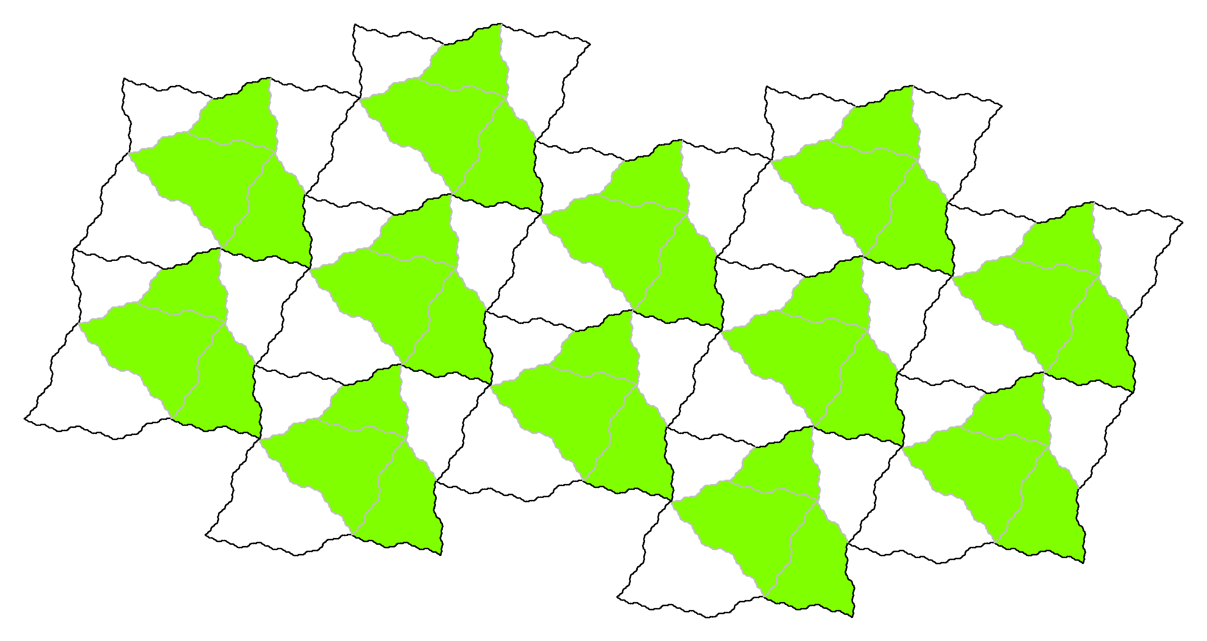
Figure 8. The Rauzy fractal ${\mathcal{R}}_{\theta_{3}}$ (black boundaries) induces a lattice tiling. The boundaries of the invariant sets within ${\mathcal{R}}_{\theta_{3}}$ are drawn in grey. The union of the invariant sets ${\mathcal{R}}_{\theta_{3}}(3)$, ${\mathcal{R}}_{\theta_{3}}(4)$, ${\mathcal{R}}_{\theta_{3}}(5)$ (coloured in green) correspond to the tent-tile ${\mathcal{F}}_{\alpha_{3}}$ by Corollary 4.4. By joining the other invariant sets across tiles in a suitable way we obtain reflections of ${\mathcal{F}}_{\alpha_{3}}$.

In particular, since $\{{\bm{\xi}}+{\mathcal{R}}_{\theta_{3}}:{\bm{\xi}}\in\Xi_{\rm lat}\}$ is a proper tiling we conclude from Lemma 3.3 that

$$\big{\{}{\bm{\xi}}+{\mathcal{R}}_{\theta_{3}}(0):{\bm{\xi}}\in\Xi_{\rm lat}\big{\}}\cup\big{\{}{\bm{\xi}}+{\mathcal{R}}_{\theta_{3}}(1):{\bm{\xi}}\in\Xi_{\rm lat}\big{\}}\cup\big{\{}{\bm{\xi}}+{\mathcal{R}}_{\theta_{3}}(2):{\bm{\xi}}\in\Xi_{\rm lat}\big{\}}\\ \cup\big{\{}{\bm{\xi}}+\big{(}{\mathcal{R}}_{\theta_{3}}(3)\cup{\mathcal{R}}_{\theta_{3}}(4)\cup{\mathcal{R}}_{\theta_{3}}(5)\big{)}:{\bm{\xi}}\in\Xi_{\rm lat}\big{\}}$$

is also a proper tiling. We apply Theorem 4.3 and Corollary 4.4 and deduce that the collection

$$\big{\{}{\bm{\xi}}+{\Psi}_{\alpha}(1)-f_{R}({\mathcal{F}}_{\alpha}):{\bm{\xi}}\in\Xi\big{\}}\cup\big{\{}{\bm{\xi}}+{\Psi}_{\alpha}(\alpha)-f_{L}\circ f_{R}({\mathcal{F}}_{\alpha}):{\bm{\xi}}\in\Xi\big{\}}\\ \cup\big{\{}{\bm{\xi}}+{\Psi}_{\alpha}(\alpha^{2})-f_{L}^{2}({\mathcal{F}}_{\alpha}):{\bm{\xi}}\in\Xi\big{\}}\cup\big{\{}{\bm{\xi}}+\mathcal{F}_{\alpha}:{\bm{\xi}}\in\Xi\big{\}}$$

is a proper tiling. Since ${\Psi}_{\alpha}(\alpha-1)$ and ${\Psi}_{\alpha}(\alpha^{2}-1)$ are lattice points we see that

$$\big{\{}{\bm{\xi}}+\big{(}({\Psi}_{\alpha}(1)-f_{R}({\mathcal{F}}_{\alpha}))\cup({\Psi}_{\alpha}(1)-f_{L}\circ f_{R}({\mathcal{F}}_{\alpha}))\cup({\Psi}_{\alpha}(1)-f_{L}^{2}({\mathcal{F}}_{\alpha}))\big{)}:{\bm{\xi}}\in\Xi\big{\}}\\ \cup\big{\{}{\bm{\xi}}+\mathcal{F}_{\alpha}:{\bm{\xi}}\in\Xi\big{\}}$$

is a proper tiling, too. Now, the statement of the theorem follows immediately by observing that

$$({\Psi}_{\alpha}(1)-f_{R}({\mathcal{F}}_{\alpha}))\cup({\Psi}_{\alpha}(1)-f_{L}\circ f_{R}({\mathcal{F}}_{\alpha}))\cup({\Psi}_{\alpha}(1)-f_{L}^{2}({\mathcal{F}}_{\alpha}))\\ ={\Psi}_{\alpha}(1)-(f_{R}({\mathcal{F}}_{\alpha})\cup f_{L}\circ f_{R}({\mathcal{F}}_{\alpha})\cup f_{L}^{2}({\mathcal{F}}_{\alpha}))={\Psi}_{\alpha}(1)-{\mathcal{F}}_{\alpha}.$$

∎

Remark 5.4.

Observe that it also follows from [2, Proposition 4.20] (in terms of automorphisms of the free group) that ${\mathcal{R}}_{\theta_{3}}$ induces a (multiple) lattice tiling. The same holds true for Theorem 5.5, Theorem 5.6 and Theorem 5.9 in an analogous way.

Theorem 5.5.

Let $\alpha=\alpha_{-1}$, $\beta=\beta(\alpha)$ and

$$\Xi:=\left\{u_{1}{\Psi}_{\alpha}(\alpha-\beta)+u_{2}{\Psi}_{\alpha}(\alpha-\beta^{2}):u_{1},u_{2}\in{\mathbb{Z}}\right\}.$$

Then

$$\dim_{H}(\partial\mathcal{F}_{\alpha})=\frac{2\log(\mu_{\rm sr})}{\log(\beta)}\approx 1.70018,$$

where $\mu_{\rm sr}\approx 1.61299$ is the dominant root of $t^{10}-t^{7}-4t^{5}-4t^{4}-t^{3}-4t^{2}-4t+1$, and the collection $\{{\bm{\xi}}+\mathcal{F}_{\alpha}:{\bm{\xi}}\in\Xi\}\cup\{{\bm{\xi}}+({\Psi}_{\alpha}(\alpha)-\mathcal{F}_{\alpha}):{\bm{\xi}}\in\Xi\}$ provides a proper tiling of the Euclidean space ${\mathbb{R}}^{2}$.

Proof.

The proof runs analogously to that of Theorem 5.3. We consider the substitution $\zeta^{\prime}_{3}$ discussed in Theorem 4.8. It is reducible, satisfies the weak coincidence condition and Condition (3.2). The dominant root of ${M}_{\zeta^{\prime}_{3}}$ is given by $\lambda_{0}=\beta=\alpha_{1}\approx 1.75488$, for the Galois conjugates we have ${\left\lvert\lambda_{1}\right\rvert}={\left\lvert\lambda_{2}\right\rvert}=\beta^{-\nicefrac{{1}}{{2}}}$. We algorithmically compute the self-replicating boundary graph $\Gamma^{(\rm sr)}_{\zeta^{\prime}_{3}}$. It turns out that the largest eigenvalue of the incidence matrix $\mu_{\rm sr}$ is as stated. As before, Corollary 3.10 immediately yield $\dim_{H}(\partial\mathcal{F}_{\alpha})$.

We algorithmically calculate the lattice boundary graph $\Gamma^{(\rm lat)}_{\zeta^{\prime}_{3}}$ and determine the largest eigenvalue of the incidence matrix $\mu_{\rm lat}=\mu_{\rm sr}<\lambda_{0}$. Therefore, the collection $\{{\bm{\xi}}+{\mathcal{R}}_{\zeta^{\prime}_{3}}:{\bm{\xi}}\in\Xi_{\rm lat}\}$ is a proper tiling. From Lemma 3.3 we deduce that the collection

$$\{{\bm{\xi}}+({\mathcal{R}}_{\zeta_{3}}(0)\cup{\mathcal{R}}_{\zeta_{3}}(1)\cup{\mathcal{R}}_{\zeta_{3}}(2)):{\bm{\xi}}\in\Xi_{\rm lat}\}\\ \cup\{{\bm{\xi}}+({\mathcal{R}}_{\zeta_{3}}(3)\cup{\mathcal{R}}_{\zeta_{3}}(4)\cup{\mathcal{R}}_{\zeta_{3}}(5)):{\bm{\xi}}\in\Xi_{\rm lat}\}$$

is also a proper tiling. We apply Theorem 4.8 and observe that ${\Psi}_{\alpha}(\alpha-\beta),{\Psi}_{\alpha}(\beta-\beta^{2})\in\Xi$. This shows that

$$\{{\bm{\xi}}+({A}_{\alpha}\mathcal{F}_{\alpha}\cup({\Psi}_{\alpha}(\beta)-{B}_{\alpha}{A}_{\alpha}\mathcal{F}_{\alpha})\cup({\Psi}_{\alpha}(\beta-\beta^{2})-{B}^{2}_{\alpha}\mathcal{F}_{\alpha})):{\bm{\xi}}\in\Xi\}\cup\\ \{{\bm{\xi}}+(({\Psi}_{\alpha}(\alpha)-{A}_{\alpha}\mathcal{F}_{\alpha})\cup({\Psi}_{\alpha}(\alpha-\beta)+{B}_{\alpha}{A}_{\alpha}\mathcal{F}_{\alpha})\cup({\Psi}_{\alpha}(\alpha-\beta+\beta^{2})-{B}^{2}_{\alpha}\mathcal{F}_{\alpha})):{\bm{\xi}}\in\Xi\}$$

is a proper tiling, too. From the observations

$${A}_{\alpha}\mathcal{F}_{\alpha}\cup({\Psi}_{\alpha}(\beta)-{B}_{\alpha}{A}_{\alpha}\mathcal{F}_{\alpha})\cup({\Psi}_{\alpha}(\beta-\beta^{2})-{B}^{2}_{\alpha}\mathcal{F}_{\alpha})\\ =f_{L}(\mathcal{F}_{\alpha})\cup f_{R}\circ f_{L}(\mathcal{F}_{\alpha})\cup f^{2}_{R}(\mathcal{F}_{\alpha})=\mathcal{F}_{\alpha},$$

$$({\Psi}_{\alpha}(\alpha)-{A}_{\alpha}\mathcal{F}_{\alpha})\cup({\Psi}_{\alpha}(\alpha-\beta)+{B}_{\alpha}{A}_{\alpha}\mathcal{F}_{\alpha})\cup({\Psi}_{\alpha}(\alpha-\beta+\beta^{2})-{B}^{2}_{\alpha}\mathcal{F}_{\alpha})\\ =({\Psi}_{\alpha}(\alpha)-f_{L}(\mathcal{F}_{\alpha}))\cup(({\Psi}_{\alpha}(\alpha)-f_{R}\circ f_{L}(\mathcal{F}_{\alpha}))\cup({\Psi}_{\alpha}(\alpha)f^{2}_{R}(\mathcal{F}_{\alpha}))={\Psi}_{\alpha}(\alpha)-\mathcal{F}_{\alpha}$$

the theorem follows immediately. ∎

Theorem 5.6.

Let $\alpha=\alpha_{-3}$, $\beta=\beta(\alpha)$ and

$$\Xi:=\left\{u_{1}{\Psi}_{\alpha}(1-\beta)+u_{2}{\Psi}_{\alpha}(1-\beta^{2}):u_{1},u_{2}\in{\mathbb{Z}}\right\}.$$

Then

$$\dim_{H}(\partial\mathcal{F}_{\alpha})=\frac{2\log(\mu_{\rm sr})}{\log(\beta)}\approx 1.25074,$$

where $\mu_{\rm sr}\approx 1.27004$ is the dominant root of $t^{10}-t^{7}-t^{3}-2t-1$, and the collection $\{{\bm{\xi}}+\mathcal{F}_{\alpha}:{\bm{\xi}}\in\Xi\}\cup\{{\bm{\xi}}+({\Psi}_{\alpha}(1)-\mathcal{F}_{\alpha}):{\bm{\xi}}\in\Xi\}$ is a proper tiling of the Euclidean space ${\mathbb{R}}^{2}$.

Proof.

We use the well-known strategy from Theorem 5.3 and Theorem 5.5. Consider the substitution $\theta^{\prime}_{3}$ discussed in Theorem 4.6. It is reducible and satisfies the weak coincidence condition as well as Condition (3.2). The dominant root of ${M}_{\theta^{\prime}_{3}}$ is given by $\lambda_{0}=\beta=\alpha_{3}\approx 1.46557$, for the Galois conjugates we have ${\left\lvert\lambda_{1}\right\rvert}={\left\lvert\lambda_{2}\right\rvert}=\beta^{-\nicefrac{{1}}{{2}}}$. We algorithmically compute the self-replicating boundary graph $\Gamma^{(\rm sr)}_{\theta^{\prime}_{3}}$ and realise that the dominant eigenvalue of its adjacency matrix $\mu_{\rm sr}$ is the dominant root of $t^{10}-t^{7}-t^{3}-2t-1$. Corollary 3.10 yields the Hausdorff dimension $\dim_{H}(\partial\mathcal{F}_{\alpha})$.

The collection $\{{\bm{\xi}}+{\mathcal{R}}_{\theta^{\prime}_{3}}:{\bm{\xi}}\in\Xi_{\rm lat}\}$ is a proper tiling since algorithmic calculation shows that $\mu_{\rm lat}=\mu_{\rm sr}<\lambda_{0}$. By observing Lemma 3.3, Theorem 4.6 and the fact that ${\Psi}_{\alpha}(1-\beta),{\Psi}_{\alpha}(\beta-\beta^{2})\in\Xi$ we see that

$$\{{\bm{\xi}}+({A}_{\alpha}\mathcal{F}_{\alpha}\cup({\Psi}_{\alpha}(\beta)-{B}_{\alpha}{A}_{\alpha}\mathcal{F}_{\alpha})\cup({\Psi}_{\alpha}(\beta-\beta^{2})-{B}^{2}_{\alpha}\mathcal{F}_{\alpha})):{\bm{\xi}}\in\Xi\}\cup\\ \{{\bm{\xi}}+(({\Psi}_{\alpha}(1)-{A}_{\alpha}\mathcal{F}_{\alpha})\cup({\Psi}_{\alpha}(1-\beta)+{B}_{\alpha}{A}_{\alpha}\mathcal{F}_{\alpha})\cup({\Psi}_{\alpha}(1-\beta+\beta^{2})-{B}^{2}_{\alpha}\mathcal{F}_{\alpha})):{\bm{\xi}}\in\Xi\}$$

is also a proper tiling. From this one easily obtains the statement from the theorem. ∎

The right hand side of Figure 2 shows the structure of the tiling induced by the tent-tile ${\mathcal{F}}_{\alpha_{-3}}$.

Two tent-tiles do not induce lattice tilings. Here we only calculate the Hausdorff dimension of the boundary which is done in the same way as in the previous theorems.

Theorem 5.7.

Let $\alpha=\alpha_{5}$. Then

$$\dim_{H}(\partial\mathcal{F}_{\alpha})=\frac{2\log(\mu_{\rm sr})}{\log(\alpha)}\approx 1.37858,$$

where $\mu_{\rm sr}\approx 1.21389$ is the dominant root of $t^{13}-t^{7}-t^{6}-2t^{4}+1$.

Proof.

We consider the substitution $\theta_{5}$. It is reducible, satisfies the strong coincidence condition but does not satisfy Condition (3.2) (therefore, ${\mathcal{R}}_{\theta^{\prime}_{5}}$ does not induce a lattice tiling). From Theorem 4.3 we see that $\lambda_{0}=\alpha\approx 1.32472$ is the dominant root of ${M}_{\theta_{5}}$. For the Galois conjugates $\lambda_{1},\lambda_{2}$ we have ${\left\lvert\lambda_{1}\right\rvert}={\left\lvert\lambda_{2}\right\rvert}=\alpha^{-\nicefrac{{1}}{{2}}}$.

We algorithmically compute the self-replicating boundary graph $\Gamma^{(\rm sr)}_{\theta_{5}}$. It turns out that the dominant eigenvalue of its adjacency matrix is the dominant root of the polynomial $t^{13}-t^{7}-t^{6}-2t^{4}+1$. For each $a\in\{0,\ldots,9\}$ the invariant set ${\mathcal{R}}_{\theta_{5}}(a)$ is an affine image of $\mathcal{F}_{\alpha}$, therefore, $\dim_{B}(\partial{\mathcal{R}}_{\theta_{5}}(a))=\dim_{B}(\partial\mathcal{F}_{\alpha})$. Now, the statement of the theorem follows immediately from Corollary 3.10. ∎

Theorem 5.8.

Let $\alpha=\alpha_{-5}$ and $\beta=\beta(\alpha)$. Then

$$\dim_{H}(\partial\mathcal{F}_{\alpha})=\frac{2\log(\mu_{\rm sr})}{\log(\beta)}\approx 1.92089,$$

where $\mu_{\rm sr}\approx 1.31007$ is the dominant root of $t^{21}-t^{20}+t^{19}-t^{18}+t^{17}-2t^{16}+t^{15}-2t^{14}+2t^{13}-3t^{12}+t^{11}+t^{9}-2t^{8}-3t^{6}-2t^{5}-2t^{4}-t^{3}-t^{2}+t+1$.

Proof.

We consider the substitution $\theta^{\prime}_{5}$. It is reducible and does not satisfy the strong coincidence condition. However, one easily verifies that the weak coincidence condition is satisfied. From Theorem 4.6 we see that $\lambda_{0}=\beta=\alpha_{5}\approx 1.32472$ is the dominant root of ${M}_{\theta^{\prime}_{5}}$. For the Galois conjugates $\lambda_{1},\lambda_{2}$ we have ${\left\lvert\lambda_{1}\right\rvert}={\left\lvert\lambda_{2}\right\rvert}=\beta^{-\nicefrac{{1}}{{2}}}$. Since Condition (3.2) is not satisfied, ${\mathcal{R}}_{\theta^{\prime}_{5}}$ does not induce a lattice tiling.

Without any problems one algorithmically calculates the self replicating boundary graph and verify that the largest eigenvalue of its incidence matrix $\mu_{\rm sr}$ is exactly as claimed. With this, $\dim_{H}(\partial\mathcal{F}_{\alpha})$ can be calculated from Corollary 3.10. ∎

5.2. Three dimensional tent-tiles

The special Pisot numbers $\alpha_{-4}$ and $\alpha_{4}$ are of algebraic degree four, thus, they induce three-dimensional tent-tiles. For both cases the other Galois conjugates consist of a real number and a complex conjugate pair of numbers. Especially, these conjugates have distinct modulus and therefore Corollary 3.10 does only yield an upper bound for the Hausdorff dimension. However, the strategy we used for showing the results for planar tent-tiles also works for the three-dimensional case.

Theorem 5.9.

Let $\alpha=\alpha_{4}$ and

$$\Xi:=\left\{u_{1}{\Psi}_{\alpha}(1-\alpha)+u_{2}{\Psi}_{\alpha}(1-\alpha^{2})+u_{3}{\Psi}_{\alpha}(1-\alpha^{3}):u_{1},u_{2},u_{3}\in{\mathbb{Z}}\right\}.$$

Then

$$\dim_{H}(\partial\mathcal{F}_{\alpha})\leq\dim_{B}(\partial\mathcal{F}_{\alpha})=3+\frac{\log(\alpha)-\log(\mu_{\rm sr})}{\log{\left\lvert\lambda_{3}\right\rvert}}\approx 2.74421,$$

where $\mu_{\rm sr}\approx 1.31162$ is the dominant root of $t^{15}-4t^{8}-2t^{6}-2t^{5}-2t^{3}-1$ and $\lambda_{3}\approx-0.81917$ is the smallest Galois conjugate (according to modulus) of $\alpha$. The collection $\{{\bm{\xi}}+\mathcal{F}_{\alpha}:{\bm{\xi}}\in\Xi\}\cup\{{\bm{\xi}}+({\Psi}_{\alpha}(1)-\mathcal{F}_{\alpha}):{\bm{\xi}}\in\Xi\}$ provides a proper tiling of the Euclidean space ${\mathbb{R}}^{3}$.

Proof.

The proof runs quite analogous to that of Theorem 5.3. We consider the substitution $\theta_{4}$ (see Theorem 4.3) which is reducible and satisfies the strong coincidence condition. The dominant root of ${M}_{\theta_{4}}$ is given by $\lambda_{0}=\alpha\approx 1.38028$, for the Galois conjugates we have ${\left\lvert\lambda_{1}\right\rvert}={\left\lvert\lambda_{2}\right\rvert}\approx 0.94044>{\left\lvert\lambda_{3}\right\rvert}\approx 0.81917$. Algorithmic computation of the self-replicating boundary graph $\Gamma^{(\rm sr)}_{\theta_{4}}$ yields $\mu_{\rm sr}\approx 1.31162$ (the dominant root of $t^{15}-4t^{8}-2t^{6}-2t^{5}-2t^{3}-1$). Now, the statement concerning the fractal dimension immediately follows from Theorem 3.9 and Corollary 3.10.

The collection $\{{\bm{\xi}}+{\mathcal{R}}_{\theta_{4}}:{\bm{\xi}}\in\Xi_{\rm lat}\}$ is a proper tiling since $\theta_{4}$ satisfies Condition (3.2) and algorithmic calculation shows that $\mu_{\rm lat}=\mu_{\rm sr}<\lambda_{0}$. From Lemma 3.3 we deduce that

$$\{{\bm{\xi}}+({\mathcal{R}}_{\theta_{4}}(0)\cup{\mathcal{R}}_{\theta_{4}}(1)\cup{\mathcal{R}}_{\theta_{4}}(2)\cup{\mathcal{R}}_{\theta_{4}}(3)):{\bm{\xi}}\in\Xi_{\rm lat}\}\\ \cup\{{\bm{\xi}}+({\mathcal{R}}_{\theta_{4}}(4)\cup{\mathcal{R}}_{\theta_{4}}(5)\cup{\mathcal{R}}_{\theta_{4}}(6)\cup{\mathcal{R}}_{\theta_{4}}(7)):{\bm{\xi}}\in\Xi_{\rm lat}\}$$

is a tiling. We observe Theorem 4.3, Corollary 4.4 and that ${\Psi}_{\alpha}(1-\alpha),{\Psi}_{\alpha}(1-\alpha^{2}),{\Psi}_{\alpha}(1-\alpha^{3})\in\Xi$ in order to see that

$$\{{\bm{\xi}}+(({\Psi}_{\alpha}(1)-f_{R}({\mathcal{F}}_{\alpha}))\cup({\Psi}_{\alpha}(1)-f_{L}\circ f_{R}({\mathcal{F}}_{\alpha}))\cup\\ ({\Psi}_{\alpha}(1)-f_{L}^{2}\circ f_{R}({\mathcal{F}}_{\alpha}))\cup({\Psi}_{\alpha}(1)-f_{L}^{3}({\mathcal{F}}_{\alpha}))):{\bm{\xi}}\in\Xi\}\cup\{{\bm{\xi}}+\mathcal{F}_{\alpha}:{\bm{\xi}}\in\Xi\}$$

is also a tiling and from this the theorem follows immediately. ∎

Theorem 5.10.

Let $\alpha=\alpha_{-4}$, $\beta=\beta(\alpha)$ and

$$\Xi:=\left\{u_{1}{\Psi}_{\alpha}(1-\beta)+u_{2}{\Psi}_{\alpha}(1-\beta^{2})+u_{3}{\Psi}_{\alpha}(1-\beta^{3}):u_{1},u_{2},u_{3}\in{\mathbb{Z}}\right\}.$$

Then

$$\dim_{H}(\partial\mathcal{F}_{\alpha})\leq\dim_{B}(\partial\mathcal{F}_{\alpha})=3+\frac{2\log(\beta)-\log(\mu_{\rm sr})}{2\log{\left\lvert\lambda_{3}\right\rvert}}\approx 2.815,$$

where $\mu_{\rm sr}\approx 1.77033$ is the dominant root of $t^{28}-2t^{27}+t^{26}-6t^{23}+2t^{22}+6t^{20}-2t^{19}+11t^{18}+t^{17}+8t^{16}-14t^{14}-12t^{13}-5t^{12}+9t^{11}+14t^{10}+8t^{9}-t^{8}-13t^{7}+4t^{6}-t^{5}-t^{3}+t^{2}-2t+1$ and $\lambda_{3}\approx-0.81917$ is the smallest Galois conjugate (according to modulus) of $\beta$. The collection $\{{\bm{\xi}}+\mathcal{F}_{\alpha}:{\bm{\xi}}\in\Xi\}$ provides a proper tiling of the Euclidean space ${\mathbb{R}}^{3}$.

Proof.

We consider the substitution $\theta^{\prime}_{4}$ discussed in Theorem 4.6. It is irreducible and satisfies the strong coincidence condition. The dominant root of ${M}_{\theta^{\prime}_{4}}$ is given by $\lambda_{0}=\beta^{2}=\alpha_{4}^{2}\approx 1.90517$. Algorithmic computation of the self-replicating boundary graph $\Gamma^{(\rm sr)}_{\theta_{4}}$ yields $\mu_{\rm sr}$ as stated. Now,the fractal dimension can be calculated with Theorem 3.9 and Corollary 3.10.

As $\theta^{\prime}_{4}$ is irreducible ${\mathcal{R}}_{\theta^{\prime}_{4}}$ induces a lattice tiling which we may assume to be proper by the Pisot conjecture. This is confirmed by Theorem 3.7 since $\mu_{\rm sr}<\lambda_{0}$. By a similar argumentation as in the previous theorems (${\Psi}_{\alpha}(\beta-\beta^{2})$ is a lattice point) we conclude that

$$\big{\{}{\bm{\xi}}+\big{(}{A}_{\alpha}\mathcal{F}_{\alpha}\cup({\Psi}_{\alpha}(\beta)-{B}_{\alpha}{A}_{\alpha}\mathcal{F}_{\alpha})\cup({\Psi}_{\alpha}(\beta)-{\Psi}_{\alpha}(\beta^{2})+{B}_{\alpha}^{2}{A}_{\alpha}\mathcal{F}_{\alpha})\\ \cup({\Psi}_{\alpha}(\beta)-{\Psi}_{\alpha}(\beta^{2})+{\Psi}_{\alpha}(\beta^{3})-{B}_{\alpha}^{3}\mathcal{F}_{\alpha})\big{)}:{\bm{\xi}}\in\Xi\big{\}}$$

is a proper tiling. By the definition of $f_{R}$ and $f_{L}$ we immediately obtain the stated result. ∎

References

- [1] S. Akiyama, M. Barge, V. Berthé, J.-Y. Lee, and A. Siegel, On the Pisot substitution conjecture, in Mathematics of Aperiodic Order, vol. 309 of Progress in Mathematics, Birkhäuser, 2015, pp. 33–72.
- [2] P. Arnoux, V. Berthé, A. Hilion, and A. Siegel, Fractal representation of the attractive lamination of an automorphism of the free group., Ann. Inst. Fourier, 56 (2006), pp. 2161–2212.
- [3] P. Arnoux and S. Ito, Pisot substitutions and Rauzy fractals, Bull. Belg. Math. Soc. Simon Stevin, 8 (2001), pp. 181–207. Journées Montoises d’Informatique Théorique (Marne-la-Vallée, 2000).
- [4] C. Bandt, Self-similar sets. III: Constructions with sofic systems., Monatsh. Math., 108 (1989), pp. 89–102.
- [5] M. Barge, The Pisot conjecture for -substitutions, Ergodic Theory Dyn. Syst., 38 (2018), pp. 444–472.
- [6] M. Barge and B. Diamond, Coincidence for substitutions of Pisot type, Bull. Soc. Math. Fr., 130 (2002), pp. 619–626.
- [7] M. Barnsley and A. Vince, Fractal tilings from iterated function systems., Discrete Comput. Geom., 51 (2014), pp. 729–752.
- [8] V. Berthé and A. Siegel, Tilings associated with beta-numeration and substitutions, Integers, 5 (2005), pp. paper a02, 46.
- [9] V. Berthé, A. Siegel, and J. Thuswaldner, Substitutions, Rauzy fractals and tilings, in Combinatorics, automata and number theory, vol. 135 of Encyclopedia Math. Appl., Cambridge Univ. Press, Cambridge, 2010, pp. 248–323.
- [10] M. Bestvina, M. Feighn, and M. Handel, The Tits alternative for . I: Dynamics of exponentially-growing automorphisms, Ann. Math. (2), 151 (2000), pp. 517–623.
- [11] V. Canterini and A. Siegel, Geometric representation of substitutions of Pisot type, Trans. Amer. Math. Soc., 353 (2001), pp. 5121–5144 (electronic).
- [12] H. Ei, S. Ito, and H. Rao, Atomic surfaces, tilings and coincidences. II. Reducible case, Ann. Inst. Fourier (Grenoble), 56 (2006), pp. 2285–2313.
- [13] N. P. Fogg, Substitutions in dynamics, arithmetics and combinatorics, vol. 1794 of Lecture Notes in Mathematics, Springer-Verlag, Berlin, 2002. Edited by V. Berthé, S. Ferenczi, C. Mauduit and A. Siegel.
- [14] M. Hollander and B. Solomyak, Two-symbol Pisot substitutions have pure discrete spectrum, Ergodic Theory Dynam. Systems, 23 (2003), pp. 533–540.
- [15] J. E. Hutchinson, Fractals and self-similarity, Indiana Univ. Math. J., 30 (1981), pp. 713–747.
- [16] S. Ito and H. Rao, Atomic surfaces, tilings and coincidence. I. Irreducible case, Israel J. Math., 153 (2006), pp. 129–155.
- [17] J. C. Lagarias, H. A. Porta, and K. B. Stolarsky, Asymmetric tent map expansions. I. Eventually periodic points, J. London Math. Soc. (2), 47 (1993), pp. 542–556.
- [18] , Asymmetric tent map expansions. II. Purely periodic points, Illinois J. Math., 38 (1994), pp. 574–588.
- [19] B. Loridant, A. Messaoudi, P. Surer, and J. M. Thuswaldner, Tilings induced by a class of cubic Rauzy fractals, Theoret. Comput. Sci., 477 (2013), pp. 6–31.
- [20] R. D. Mauldin and S. C. Williams, Hausdorff dimension in graph directed constructions, Trans. Amer. Math. Soc., 309 (1988), pp. 811–829.
- [21] H. Rao, Z.-Y. Wen, and Y.-M. Yang, Dual systems of algebraic iterated function systems, Adv. Math., 253 (2014), pp. 63–85.
- [22] G. Rauzy, Nombres algébriques et substitutions, Bull. Soc. Math. France, 110 (1982), pp. 147–178.
- [23] K. Scheicher, V. F. Sirvent, and P. Surer, Dynamical properties of the tent map., J. Lond. Math. Soc., II. Ser., 93 (2016), pp. 319–340.
- [24] A. Siegel and J. M. Thuswaldner, Topological properties of Rauzy fractals, Mém. Soc. Math. Fr. (N.S.), (2009), p. 140.
- [25] V. F. Sirvent and Y. Wang, Self-affine tiling via substitution dynamical systems and Rauzy fractals, Pacific J. Math., 206 (2002), pp. 465–485.
- [26] C. J. Smyth, There are only eleven special Pisot numbers, Bull. London Math. Soc., 31 (1999), pp. 1–5.