marginparsep has been altered.
topmargin has been altered.
marginparpush has been altered.
The page layout violates the ICML style.
Please do not change the page layout, or include packages like geometry,
savetrees, or fullpage, which change it for you.
We’re not able to reliably undo arbitrary changes to the style. Please remove
the offending package(s), or layout-changing commands and try again.
Physics-Informed Deep B-Spline Networks for Dynamical Systems
Zhuoyuan Wang 1 Raffaele Romagnoli 2 Jasmine Ratchford 3 Yorie Nakahira 1
Abstract
Physics-informed machine learning provides an approach to combining data and governing physics laws for solving complex partial differential equations (PDEs). However, efficiently solving PDEs with varying parameters and changing initial conditions and boundary conditions (ICBCs) with theoretical guarantees remains an open challenge. We propose a hybrid framework that uses a neural network to learn B-spline control points to approximate solutions to PDEs with varying system and ICBC parameters. The proposed network can be trained efficiently as one can directly specify ICBCs without imposing losses, calculate physics-informed loss functions through analytical formulas, and requires only learning the weights of B-spline functions as opposed to both weights and basis as in traditional neural operator learning methods. We provide theoretical guarantees that the proposed B-spline networks serve as universal approximators for the set of solutions of PDEs with varying ICBCs under mild conditions and establish bounds on the generalization errors in physics-informed learning. We also demonstrate in experiments that the proposed B-spline network can solve problems with discontinuous ICBCs and outperforms existing methods, and is able to learn solutions of 3D dynamics with diverse initial conditions.
1 Introduction
Recent advances in scientific machine learning have boosted the development for solving complex partial differential equations (PDEs). Physics-informed neural networks (PINNs) are proposed to combine information of available data and the governing physics model to learn the solutions of PDEs (Raissi et al., 2019; Han et al., 2018). However, in the real world the parameters for the PDE and for the initial and boundary conditions (ICBCs) can be changing, and solving PDEs for all possible parameters can be important but demanding. For example in a safety-critical control scenario, the system dynamics and the safe region can vary over time, resulting in changing parameters for the PDE that characterizes the probability of safety. On the other hand, solving such PDEs is important for safe control but can be hard to achieve in real time with limited online computation. In general, to account for parameterized PDEs and varying ICBCs in PINNs is challenging, as the solution space becomes much larger (Karniadakis et al., 2021). To tackle this challenge, parameterized PINNs are proposed (Cho et al., 2024). Plus, a new line of research on neural operators is conducted to learn operations of functions instead of the value of one specific function (Kovachki et al., 2023; Li et al., 2020; Lu et al., 2019). However, these methods are often computationally expensive, and the trained networks do not necessarily comply with ICBCs. On the other hand, the existing literature has empirically shown the effectiveness of neural networks with embedded B-spline structure for interpolating a single PDE Doległo et al. (2022); Zhu et al. (2024), while theoretical properties and generalization of representing multiple PDEs remain an open challenge.
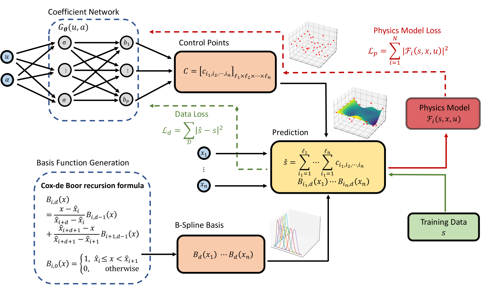
In this work, we integrate B-spline functions and physics-informed learning to form physics-informed deep B-spline networks (PI-DBSN) that can efficiently learn parameterized PDEs with varying initial and boundary conditions (Fig. 1). We provide theoretical results that bound the approximation error and generation error of PI-DBSN in learning a set of multiple PDEs with varying ICBCs. Specifically, the network composites of B-spline basis functions, and a parameterized neural network that learns the weights for the B-spline basis. The coefficient network takes inputs of the PDE and ICBC parameters, and outputs the control points tensor (i.e., weights of B-splines). Then this control points tensor is multiplied with the B-spline basis to produce the final output as the approximation of PDEs. One can evaluate the prediction of the PDE solution at any point, and we use physics loss and data loss to train the network similar to PINNs (Cuomo et al., 2022). We constrain the network output to satisfy physics laws through physics-informed losses, but use a novel B-spline formulation for more efficient learning for families of PDEs. To the best of our knowledge, this is the first work that leverages B-spline basis representation with physics-informed learning to solve PDEs with theoretical guarantees on approximation and generalization error bounds. There are several advantages for the proposed PI-DBSN framework:
-
1.
The B-spline basis functions are fixed and can be pre-calculated before training, thus we only need to train the coefficient network which saves computation and stabilizes training.
-
2.
The B-spline functions have analytical expressions for its gradients and higher-order derivatives, which provide faster and more accurate calculation for the physics-informed losses during training over automatic differentiation.
-
3.
Due to the properties of B-splines, we can directly specify Dirichlet boundary conditions and initial conditions through the control points tensor without imposing loss functions, which helps with learning extreme and complex ICBCs.
The rest of the paper is organized as follows. We discuss related work in Sec. 2, and introduce our proposed PI-DBSN in Sec. 3. We then show in Sec. 4 that despite the use of fixed B-spline basis, the PI-DBSN is a universal approximator and can learn high-dimensional PDEs. Following the theoretical analysis, in Sec. 5 we demonstrate with experiments that PI-DBSN can solve problems with discontinuous ICBCs and outperforms existing methods, and is able to learn high-dimensional PDEs. Finally, we conclude the paper in Sec. 6.
2 Related Work
PINNs: Physics-informed neural networks (PINNs) are neural networks that are trained to solve supervised learning tasks while respecting any given laws of physics described by general nonlinear partial differential equations (Raissi et al., 2019; Han et al., 2018; Cuomo et al., 2022). PINNs take both data and the physics model of the system into account, and are able to solve the forward problem of getting PDE solutions, and the inverse problem of discovering underlying governing PDEs from data. PINNs have been widely used in power systems (Misyris et al., 2020), fluid mechanics (Cai et al., 2022) and medical care (Sahli Costabal et al., 2020), etc. Different variants of PINN have been proposed to meet different design criteria, for example Bayesian PINNs are used for forward and inverse PDE problems with noisy data (Yang et al., 2021), PINNs with hard constraints are proposed to solve topology optimizations (Lu et al., 2021b), and parallel PINNs via domain decomposition are proposed to solve multi-scale and multi-physics problems (Shukla et al., 2021). It is shown that under certain assumptions that PINNs have bounded error and converge to the ground truth solutions (De Ryck & Mishra, 2022; Mishra & Molinaro, 2023; 2022; Fang, 2021; Pang et al., 2019; Jiao et al., 2021). Physics-informed learning is also used to train convolutional neural networks (CNNs) with Hermite spline kernels in Wandel et al. (2022) to provide forward-time prediction in PDEs. In comparison, our work learns solutions on the entire state-time domain leveraging the fact that B-spline control points can be directly determined for initial and Dirichlet boundary conditions without training, with theoretical guarantees on approximation and generalization error bounds.
B-splines + NN: B-splines are piece-wise polynomial functions derived from slight adjustments of Bezier curves, aimed at obtaining polynomial curves that tie together smoothly (Ahlberg et al., 2016). B-splines have been widely used in signal and imaging processing (Unser, 1999; Lehmann et al., 2001), computer aided design (Riesenfeld, 1973; Li, 2020), etc. B-splines are also used to assist in solving PDEs. For example, B-splines are used in combination with finite element methods in Jia et al. (2013); Shen et al. (2023), and are used to solve PDEs through variational dual formulation in Sukumar & Acharya (2024), splines are used to parameterize the domain of PDEs in Falini et al. (2023), and spline-inspired mesh movement networks are proposed to solve PDEs in Song et al. (2022). B-splines together with neural networks (NNs) are used for surface reconstruction (Iglesias et al., 2004), nonlinear system modeling (Yiu et al., 2001; Wang et al., 2022b), image segmentation Cho et al. (2021), and controller design for dynamical systems (Chen et al., 2004; Deng et al., 2008). Kolmogorov–Arnold Networks (KANs) (Liu et al., 2024) uses spline functions to produce learnable weights in neural networks, as an alternative architecture to multi-layer perceptrons. In comparison, the proposed neural network can take arbitrary MLP/non-MLP based architectures including KANs. NNs are also used to learn weights for B-spline functions to approximate fixed ODEs Fakhoury et al. (2022); Romagnoli et al. (2024) and fixed PDEs Doległo et al. (2022); Zhu et al. (2024). These works do not leverage the model information or PDE constraints, thus do not generalize beyond the regions with available data. Additionally, while these works only show empirical results for learning a single PDE for fixed ICBCs, we provide both theoretical guarantees, along with empirical evidence, in the approximation and generation results in learning the set of multiple PDEs of different ICBCs.
Other network design: Neural operators—such as DeepONets (Lu et al., 2019; 2021a) and Fourier Neural Operators (FNOs) (Li et al., 2020)—have been extensively studied (Kovachki et al., 2023; Lu et al., 2022). In Wang et al. (2021) DeepONets are combined with physics-informed learning to solve fixed PDEs. Generalizations of DeepONet (Gao et al., 2021) and FNO (Li et al., 2024) consider learning (state) parameterized PDEs with fast evaluation. Multi-task mechanism is incorporated within DeepONet in Kumar et al. (2024) to learn PDEs with varying ICBC, but special and manually designed polynomial representations of the varying parameter is needed as input to the branch net of the system. As DeepONet-based methods need to train two networks at a time (branch and trunk net in the architecture), the training can be unstable. Besides, any method that imposes losses on ICBCs such as DeepONets and FNOs requires additional computation in training, and the trained network may not always comply to initial and boundary conditions Brecht et al. (2023). In comparison, our method directly specifies ICBCs, and uses fixed B-spline functions as the basis such that only one coefficient network needs to be trained. This results in better compliance with initial and boundary conditions (Fig. 2), reduced training time (Table 1), and stable and efficient training (Fig. 3).
3 Proposed Method
3.1 Problem Formulation
The goal of this paper is to efficiently estimate high-dimensional surfaces with corresponding governing physics laws of a wide range variety of parameters (e.g., the solution of a family of ODEs/PDEs). We denote as the ground truth, i.e., is the value of the surface at point , where . We assume the physics laws can be written as
| (1) |
where is the parameters of the physics systems, is the number of governing equations, parameterized by is the region that the -th physics law applies. We denote the general region of interest, and in this paper we consider -dimensional bounded domain .111Such domain configuration is widely considered in the literature Takamoto et al. (2022); Gupta & Brandstetter (2022); Li et al. (2020); Raissi et al. (2019); Wang et al. (2021); Zhu et al. (2024). Our goal is to generate with neural networks to estimate on the entire domain of , with all possible parameters and . For example, in the case of solving 2D heat equations on at time with varying coefficient and , we have the physics laws to be
| (2) | |||
| (3) |
where and , and is the boundary of . Here, equation 2 is the heat equation and equation 3 is the boundary condition. In this case, we want to solve for on for all and . Similar problems have been studied in Li et al. (2024); Gao et al. (2021); Cho et al. (2024) while the majority of the literature considers solving parameterized PDEs but with either fixed coefficients or fixed domain and initial/boundary conditions. We slightly generalize the problem to consider systems with varying parameters, and with potential varying domains and initial/boundary conditions.
3.2 B-Splines with Basis Functions
In this section, we introduce one-dimensional B-splines. For state space , the B-spline basis functions are given by the Cox-de Boor recursion formula:
| (4) |
and
| (5) |
Here, denotes the value of the -th B-spline basis of order evaluated at , and is a non-decreasing vector of knot points. Since a B-spline is a piece-wise polynomial function, the knot points determine in which polynomial the parameter belongs. While there are multiple ways of choosing knot points, we use with and , and for the remaining knot points we select equispaced values. For example on with number of control points and order , we have , in total knot points.
We then define the control points
| (6) |
and the B-spline basis functions vector
| (7) |
Then, we can approximate a solution with
| (8) |
Note that with our choice of knot points, we ensure the initial and final values of coincide with the initial and final control points and . This property will be used later to directly impose initial conditions and Dirichlet boundary conditions with PI-DBSN.
3.3 Multi-Dimensional B-splines
Now we extend the B-spline scheme to the multi-dimensional case. We start by considering the 2D case where . Along each dimension , we can generate B-spline basis functions based on the Cox-de Boor recursion formula in equation 4 and equation 5. We denote the B-spline basis of order as , for the -th and -th function of and , respectively. Then with a control points matrix , the 2-dimensional surface can be approximated by the B-splines as
| (9) |
where and are the number of control points along the 2 dimensions. This can be written in the matrix multiplication form as
| (10) | ||||
where is the approximation of the 2D solution at , is the control points matrix and and are the B-spline vectors defined in equation 7.
More generally, for a -dimensional space , we can generate B-spline basis functions based on the Cox-de Boor recursion formula along each dimension with order for , and the -dimensional control point tensor will be given by , where is the -th index of the control point, and is the number of control points along the -th dimension. We can then approximate the -dimensional surface with B-splines and control points via
| (11) | ||||
3.4 Physics-Informed B-Spline Nets
In this section, we introduce our proposed physics-informed deep B-spline networks (PI-DBSN). The overall diagram of the network is shown in Fig. 1. The network composites a coefficient network that learns the control point tensor with system parameters and ICBC parameters , and the B-spline basis functions of order for . During the forward pass, the control point tensor output from the coefficient net is multiplied with the B-spline basis functions via equation 11 to get the approximation . For the backward pass, two losses are imposed to efficiently and effectively train PI-DBSN. We first impose a physics model loss
| (12) |
where is the governing physics model of the system as defined in equation 1, and is the set of points sampled to evaluated the governing physics model. When data is available, we can additionally impose a data loss
| (13) |
to capture the mean square error of the approximation, where is the data point for the high dimensional surface, is the data set, and is the prediction from the PI-DBSN. The total loss is given by
| (14) |
where and are the weights for physics and data losses, and are usually set to values close to 1.222Ablation experiments on the effects of weights for physics and data losses can be found in Appendix D.4. We use to denote the PI-DBSN parameterized by , where is the input to the coefficient net (parameters of the system and ICBCs), and will be the input to the PI-DBSN (the state and time in PDEs). With this notation we have and .
Note that several good properties of B-splines are leveraged in PI-DBSN.
First, the derivatives of the B-spline functions can be analytically calculated. Specifically, the -th derivative of the -th ordered B-spline is given by (Butterfield, 1976)
| (15) | ||||
Given this, we can directly calculate these values for the back-propagation of physics model loss , which improves both computation efficiency and accuracy over automatic differentiation that is commonly used in physic-informed learning (Cuomo et al., 2022).
Besides, any Dirichlet boundary conditions and initial conditions can be directly assigned via the control points tensor without any learning involved. This is due to the fact that the approximated solution at the end points along each axis will have the exact value of the control point. For example, in a 2D case when the initial condition is given by , we can set the first column of the control points tensor for all and this will ensure the initial condition is met for the PI-DBSN output. This greatly enhances the accuracy of the learned solution near initial and boundary conditions, and improves the ease of design for the loss function as weight factors are often used to impose stronger initial and boundary condition constraints in previous literature (Wang et al., 2022a). We will demonstrate later in the experiment section where we compare the proposed PI-DBSN with physic-informed DeepONet that this feature will result in better estimation of the PDEs when the initial and boundary conditions are hard to learn.
Furthermore, better training stability can be obtained. The B-spline basis functions are fixed and can be calculated in advance, and training is involved only for the coefficient net.
4 Theoretical Analysis
In this section, we provide theoretical guarantees of the proposed PI-DBSN on learning high-dimensional PDEs. We first show that B-splines are universal approximators, and then show that with combination of B-splines and neural networks, the proposed PI-DBSN is a universal approximator under certain conditions. At last we argue that when the physics loss is densely imposed and the loss functions are minimized, the network can learn unique PDE solutions. All theorem proofs can be found the in the Appendix of the paper.
We first consider the one-dimensional function space with norm defined over the interval . For two functions , we define the inner product of these two functions as
| (16) |
where denotes the conjugate complex. We say a function is square-integrable if the following holds
| (17) |
We define the norm between two functions as
| (18) |
We then state the following theorem that shows B-spline functions are universal approximators in the sense of norms in one dimension.
Theorem 4.1.
Given a positive natural number and any -time differentiable function , then for any , there exist a positive natural value , and a realization of control points such that
| (19) |
where
is the B-spline approximation with being the B-spline basis functions defined in equation 7.
Now that we have the error bound of B-spline approximations in one dimension, we will extend the results to arbitrary dimensions. We point out that the space is a Hilbert space (Balakrishnan, 2012). Let us consider Hilbert spaces for . We define the inner products of two -dimensional functions as
| (20) |
and we say a function is square-integrable if
| (21) |
Now we present the following lemma to bound the approximation error of -dimensional B-splines.
Lemma 4.2.
Given a set positive natural numbers and a -time differentiable function . Assume , then given any , there exist of control points for each component , such that
| (22) |
where
| (23) | ||||
On the other hand, we know that neural networks are universal approximators (Hornik et al., 1989; Leshno et al., 1993), i.e., with large enough width or depth a neural network can approximate any function with arbitrary precision. We first show that given some basic assumptions on the solution of the physics problems, the optimal control points are continuous in the system and domain parameters and , thus can be approximated by neural networks. We then restate the universal approximation theorem in our context assuming the requirements for the neural network are met. 333The Borel space assumptions are met since we consider space which is a Borel space.
Assumption 4.3.
The solution of the physics problem defined in equation 1 is continuous in and . Specifically, let and be the solutions of the physics problem with parameters and . For any , there exist and such that given , and , we have .444Under necessary domain mapping when .
Assumption 4.4.
The solution of the physics problem defined in equation 1 is differentiable in .
Assumption 4.3 is a basic assumption for a neural network to approximate solutions of families of parameterized PDEs, and is not strict as it holds for many PDE problems.555For a well-posed and stable system with unique solution (e.g., linear Poisson, convection-diffusion and heat equations with appropriate ICBCs), change of the system parameter or the ICBC parameter usually results in slight change of the value of the solution Treves (1962). Assumption 4.4 holds for many PDE problems (Chen et al., 2018; De Angelis, 2015; Barles et al., 2010), and our theoretical results can be generalized to cases where the solution is not differentiable at finite number of points.
In this following lemma, we show that with the assumptions, the optimal control points are continuous in terms of the system and ICBC parameters. Follow by that, we restate universal approximation theorem of neural networks for optimal control points.
Lemma 4.5.
For any and two -dimensional surfaces being the solution of the physics problem defined in equation 1 with parameters and . Assume Assumption 4.3 and Assumption 4.4 hold. Let and be the two control points tensors that reconstruct and . For any , , there exist such that , and , and control points tensors and with such that , , and . Here when .
Theorem 4.6.
Theorem 4.7.
Assume Assumption 4.3 and 4.4 hold. For any dimension, any and in a finite parameter set, let be the order of B-spline basis for dimension . Then for any -time differentiable function with where the domain depends on and the function depends on , and any , there exist a PI-DBSN configuration with enough width and depth, and corresponding parameters independent of and such that
| (25) |
where is the B-spline approximation defined in equation 11 with the control points tensor .
Theorem 4.7 tells us the proposed PI-BDSN is an universal appproximator of high-dimensional surfaces with varying parameters and domains. Thus we know that when the solution of the problem defined in equation 1 is unique, and the physics-informed loss functions is densely imposed and attains zero (De Ryck & Mishra, 2022; Mishra & Molinaro, 2023), we learn the solution of the PDE problem of arbitrary dimensions.
Based on these results, we also provide generalization error analysis of PI-DBSN, which can be found in Appendix B.2.
5 Experiments
In this section, we present simulation results on estimating the recovery probability of a dynamical system which gives irregular ICBCs, and on estimating the solution of 3D Heat equations with varying initial conditions. We also adapted several benchmark problems in PDEBench Takamoto et al. (2022) to account for varying system and ICBC parameters, and show generalization to non-rectangular domains. The additional results can be found in Appendix E and Appendix F.
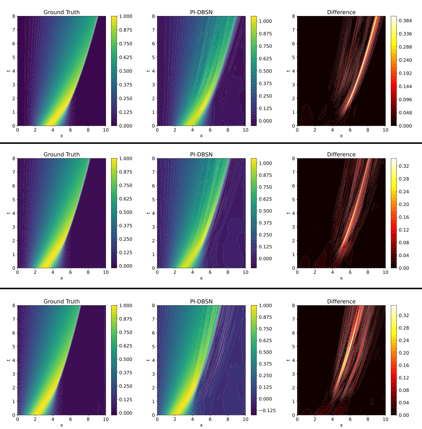
5.1 Recovery Probabilities
We consider an autonomous system with dynamics
| (26) |
where is the state, is the standard Wiener process with , and is the system parameter. Given a set
| (27) |
we want to estimate the probability of reaching at least once within time horizon starting at some . Here, is the varying parameter of the set . Mathematically this can be written as
| (28) |
From Chern et al. (2021) we know that such probability is the solution of convection-diffusion equations with certain initial and boundary conditions
| PDE: | (29) | |||
| ICBC: | (30) |
where is the complement of , and for some of interest. Note that the initial condition and boundary condition at is not continuous,666When on the boundary of the , the recovery probability at horizon is , but close to the boundary with very small the recovery probability is . which imposes difficulty for learning the solutions.
| Method | Computation Time (s) |
| PI-DBSN | 370.48 |
| PINN | 809.86 |
| PI-DeepONet | 1455.16 |
| Number of Control Points | 2 | 5 | 10 | 15 | 20 | 25 |
| Number of NN Parameters | 4417 | 5392 | 9617 | 17092 | 27817 | 41792 |
| Training Time (s) | 241.76 | 223.53 | 247.39 | 295.67 | 310.83 | 370.48 |
| Prediction MSE () | 5357.9 | 7.327 | 7.313 | 5.817 | 4.490 | 3.064 |
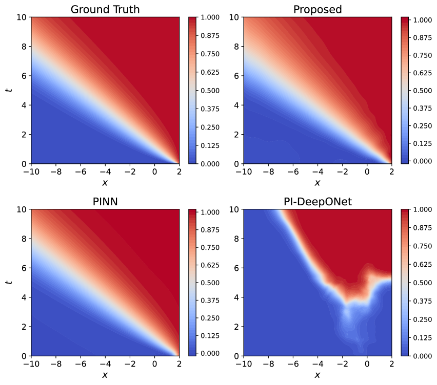
We train PI-DBSN with 3-layer fully connected neural networks with ReLU activation on varying parameters and , and test on randomly selected parameters in the same domain. We compare PI-DBSN with physics-informed neural network (PINN) (Cuomo et al., 2022) and physics-informed DeepONet (PI-DeepONet) (Goswami et al., 2023) with similar NN configurations.777Details of the configuration can be found in Appendix C. We did not compare with FNO as it is significantly more computationally expensive ( training time per epoch Li et al. (2020) compared to PI-DBSN), while our focus is fast and accurate learning. We did not compare with exhaustive variants of PI-DeepONet as our innovation is on the fundamental structure of the network, which is directly comparable with PI-DeepONet and PINN. Fig. 2 visualizes the prediction results. It can be seen that both PI-DBSN and PINN can approximate the ground truth value accurately, while PI-DeepONet fails to do so. The possible reason is that PI-DeepONet can hardly capture the initial and boundary conditions correctly when the parameter set is relatively large. Besides, with standard implementation of PI-DeepONet, the training tends to be unstable, and special training schemes such as the ones mentioned in Lee & Shin (2024) might be needed for finer results. The mean squared error (MSE) of the prediction are (Proposed PI-DBSN), (PINN), and (PI-DeepONet).
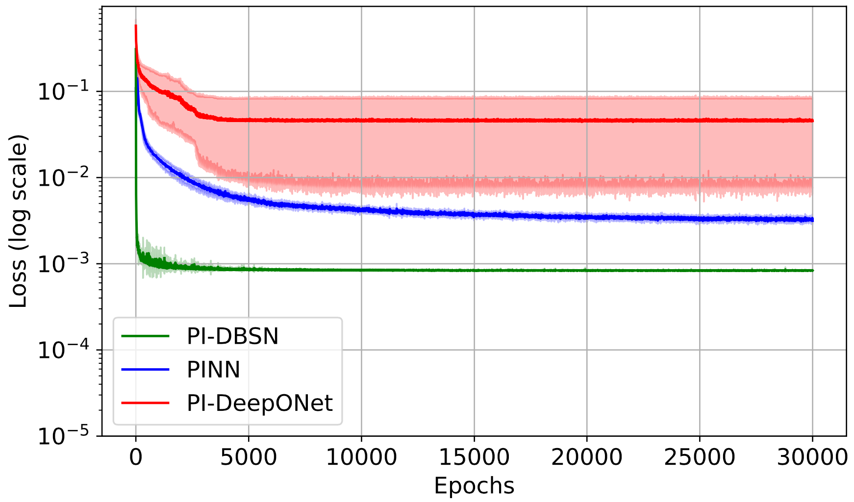
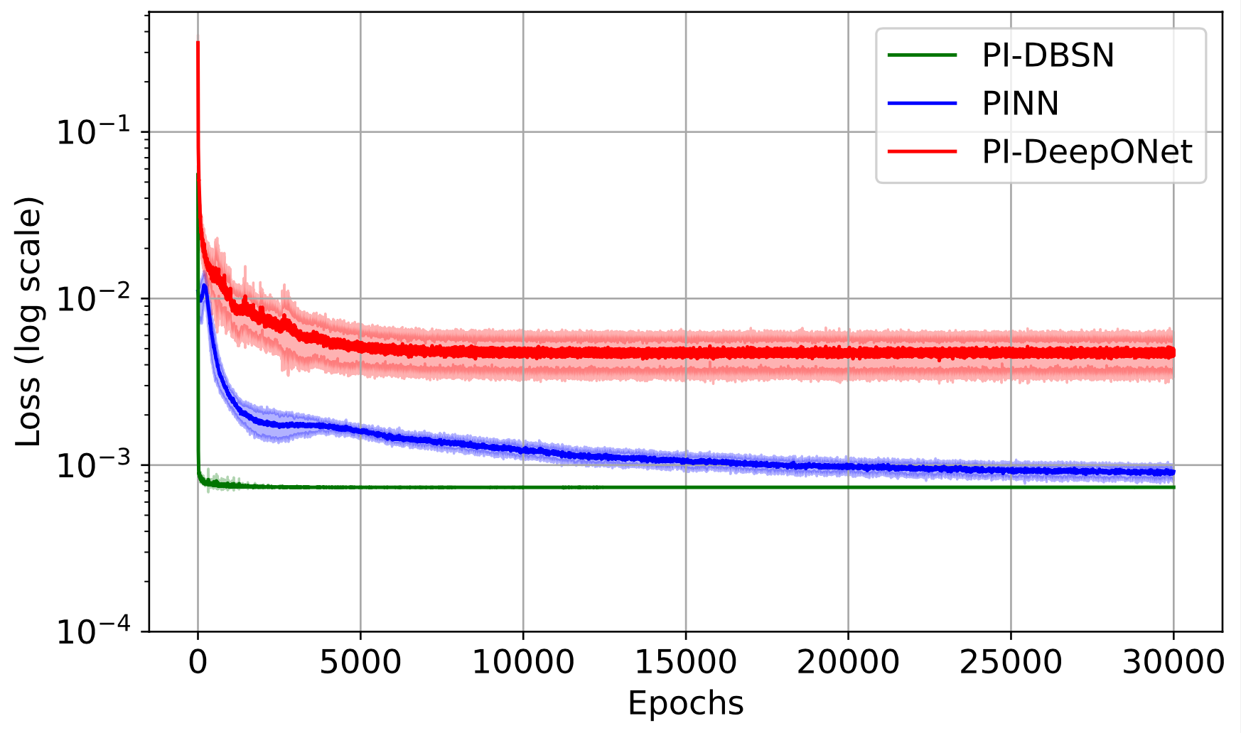
We then compare the training speed and computation time for the three methods, as shown in Fig. 3 and Table 1. We can see that the loss for PI-DBSN drops the fastest and reaches convergence in the shortest amount of time. This is because PI-DBSN has a relatively smaller NN size with the fixed B-spline basis, and achieves zero initial and boundary condition losses at the very beginning of the training. Besides, thanks to the analytical calculation of gradients and Hessians, the training time of PI-DBSN is the shortest among all three methods.
We also investigate the effect of the number of control points on the performance of PI-DBSN. Table 2 shows the approximation error and training time of PI-DBSN with different numbers of control points along each dimension. We can see that the training time increases as the number of control points increases, and the approximation error decreases, which matches with Theorem 4.7 which indicates more control points can result in less approximation error.
Experiment details and additional experiment results to verify the derivative calculations from B-splines and the optimality of the control points can be found in the Appendix.
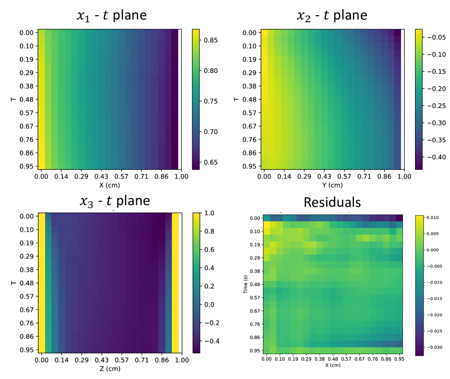
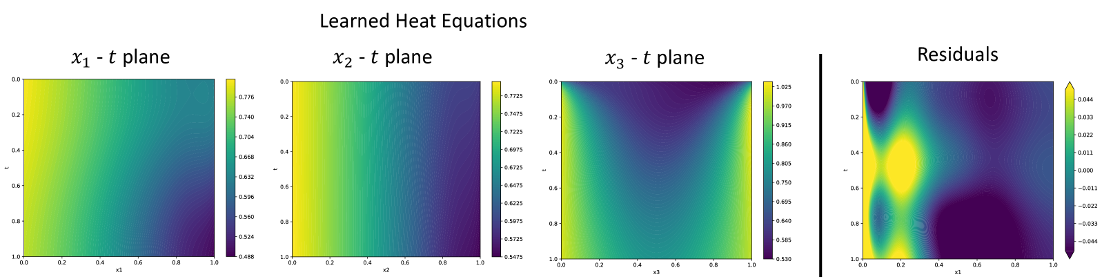
5.2 3D Heat Equations
We consider the 3D heat equation given by
| (31) |
where is the constant diffusion coefficient. Here are the states, and the domains of interest are , and . All lengths are in centimeters () and the time is in seconds (). In this experiment we solve equation 31 with random linear initial conditions:
| (32) |
where and are randomly chosen. We impose the following Dirichlet and Neumann boundary conditions:
| (33) | ||||
| (34) |
We train PI-DBSN on varying with control points along each dimension. Detailed training configurations can be found in the Appendix of the paper. Fig. 4 shows the learned heat equation and a slice of the residual in the - plane. It can be seen that the value is diffusing over time as intended. Although our initial condition does not adhere to the heat equation as estimated by the B-spline derivative, we quickly achieve a low residual. The average residuals during training and testing are and , which indicates the efficacy of the PI-DBSN method.888This is lower than the PINN testing residual . See Appendix C.6 for details.
6 Conclusion
In this paper, we consider the problem of learning solutions of PDEs with varying system parameters and initial and boundary conditions. We propose physics-informed deep B-spline networks (PI-DBSN), which incorporate B-spline functions into neural networks, to efficiently solve this problem. The advantages of the proposed PI-DBSN is that it can produce accurate analytical derivatives over automatic differentiation to calculate physics-informed losses, and can directly impose initial conditions and Dirichlet boundary conditions through B-spline coefficients. We prove theoretical guarantees that PI-DBSNs are universal approximators and under certain conditions can reconstruct PDEs of arbitrary dimensions. We then demonstrate in experiments that PI-DBSN performs better than existing methods on learning families of PDEs with discontinuous ICBCs, and has the capability of addressing higher dimensional problems.
For limitations and future work, we point out that even though B-splines are arguably a more efficient representation of the PDE problems, the PI-DBSN method still suffers from the curse of dimensionality. Specifically, the number of control points scales exponentially with the dimension of the problem, and as our theory and experiment suggest denser control points will help with obtaining lower approximation error. Besides, while the current formulation only allows regular geometry for the domain of interest, diffeomorphism transformations and non-uniform rational B-Splines (NURBS) (Piegl & Tiller, 2012) can be potentially applied to generalize the framework to irregular domains. How to further exploit the structure of the problem and learn large solution spaces in high dimensions with sparse data in complex domains are exciting future directions.
Acknowledgement
Copyright 2024 Carnegie Mellon University and Duquesne University
This material is based upon work funded and supported by the Department of Defense under Contract No. FA8702-15-D-0002 with Carnegie Mellon University for the operation of the Software Engineering Institute, a federally funded research and development center.
The view, opinions, and/or findings contained in this material are those of the author(s) and should not be construed as an official Government position, policy, or decision, unless designated by other documentation.
[DISTRIBUTION STATEMENT A] This material has been approved for public release and unlimited distribution. Please see Copyright notice for non-US Government use and distribution.
This work is licensed under a Creative Commons Attribution-NonCommercial 4.0 International License. Requests for permission for non-licensed uses should be directed to the Software Engineering Institute at permission@sei.cmu.edu.
DM25-0262
This paper presents work whose goal is to advance the field of Machine Learning. There are many potential societal consequences of our work, none which we feel must be specifically highlighted here.
References
- Ahlberg et al. (2016) Ahlberg, J. H., Nilson, E. N., and Walsh, J. L. The Theory of Splines and Their Applications: Mathematics in Science and Engineering: A Series of Monographs and Textbooks, Vol. 38, volume 38. Elsevier, 2016.
- Balakrishnan (2012) Balakrishnan, A. V. Applied Functional Analysis: A, volume 3. Springer Science & Business Media, 2012.
- Barles et al. (2010) Barles, G., Chasseigne, E., and Imbert, C. Hölder continuity of solutions of second-order non-linear elliptic integro-differential equations. Journal of the European Mathematical Society, 13(1):1–26, 2010.
- Blu & Unser (1999) Blu, T. and Unser, M. Quantitative fourier analysis of approximation techniques. i. interpolators and projectors. IEEE Transactions on signal processing, 47(10):2783–2795, 1999.
- Brecht et al. (2023) Brecht, R., Popovych, D. R., Bihlo, A., and Popovych, R. O. Improving physics-informed deeponets with hard constraints. arXiv preprint arXiv:2309.07899, 2023.
- Butterfield (1976) Butterfield, K. R. The computation of all the derivatives of a b-spline basis. IMA Journal of Applied Mathematics, 17(1):15–25, 1976.
- Cai et al. (2022) Cai, S., Mao, Z., Wang, Z., Yin, M., and Karniadakis, G. E. Physics-informed neural networks (pinns) for fluid mechanics: A review. Acta Mechanica Sinica, pp. 1–12, 2022.
- Chen et al. (2018) Chen, J., Huang, M., Rasila, A., and Wang, X. On lipschitz continuity of solutions of hyperbolic poisson’s equation. Calculus of Variations and Partial Differential Equations, 57:1–32, 2018.
- Chen et al. (2004) Chen, Y., Moore, K. L., and Bahl, V. Learning feedforward control using a dilated b-spline network: Frequency domain analysis and design. IEEE Transactions on neural networks, 15(2):355–366, 2004.
- Chern et al. (2021) Chern, A., Wang, X., Iyer, A., and Nakahira, Y. Safe control in the presence of stochastic uncertainties. In 2021 60th IEEE Conference on Decision and Control (CDC), pp. 6640–6645. IEEE, 2021.
- Cho et al. (2021) Cho, M., Balu, A., Joshi, A., Deva Prasad, A., Khara, B., Sarkar, S., Ganapathysubramanian, B., Krishnamurthy, A., and Hegde, C. Differentiable spline approximations. Advances in neural information processing systems, 34:20270–20282, 2021.
- Cho et al. (2024) Cho, W., Jo, M., Lim, H., Lee, K., Lee, D., Hong, S., and Park, N. Parameterized physics-informed neural networks for parameterized pdes. arXiv preprint arXiv:2408.09446, 2024.
- Cuomo et al. (2022) Cuomo, S., Di Cola, V. S., Giampaolo, F., Rozza, G., Raissi, M., and Piccialli, F. Scientific machine learning through physics–informed neural networks: Where we are and what’s next. Journal of Scientific Computing, 92(3):88, 2022.
- De Angelis (2015) De Angelis, T. A note on the continuity of free-boundaries in finite-horizon optimal stopping problems for one-dimensional diffusions. SIAM Journal on Control and Optimization, 53(1):167–184, 2015.
- De Ryck & Mishra (2022) De Ryck, T. and Mishra, S. Error analysis for physics-informed neural networks (pinns) approximating kolmogorov pdes. Advances in Computational Mathematics, 48(6):79, 2022.
- Deng & Lin (2014) Deng, C. and Lin, H. Progressive and iterative approximation for least squares b-spline curve and surface fitting. Computer-Aided Design, 47:32–44, 2014.
- Deng et al. (2008) Deng, H., Oruganti, R., and Srinivasan, D. Neural controller for ups inverters based on b-spline network. IEEE Transactions on Industrial Electronics, 55(2):899–909, 2008.
- Doległo et al. (2022) Doległo, K., Paszyńska, A., Paszyński, M., and Demkowicz, L. Deep neural networks for smooth approximation of physics with higher order and continuity b-spline base functions. arXiv preprint arXiv:2201.00904, 2022.
- Fakhoury et al. (2022) Fakhoury, D., Fakhoury, E., and Speleers, H. Exsplinet: An interpretable and expressive spline-based neural network. Neural Networks, 152:332–346, 2022.
- Falini et al. (2023) Falini, A., D’Inverno, G. A., Sampoli, M. L., and Mazzia, F. Splines parameterization of planar domains by physics-informed neural networks. Mathematics, 11(10):2406, 2023.
- Fang (2021) Fang, Z. A high-efficient hybrid physics-informed neural networks based on convolutional neural network. IEEE Transactions on Neural Networks and Learning Systems, 33(10):5514–5526, 2021.
- Fazlyab et al. (2019) Fazlyab, M., Robey, A., Hassani, H., Morari, M., and Pappas, G. Efficient and accurate estimation of lipschitz constants for deep neural networks. Advances in neural information processing systems, 32, 2019.
- Gao et al. (2021) Gao, H., Sun, L., and Wang, J.-X. Phygeonet: Physics-informed geometry-adaptive convolutional neural networks for solving parameterized steady-state pdes on irregular domain. Journal of Computational Physics, 428:110079, 2021.
- Goswami et al. (2023) Goswami, S., Bora, A., Yu, Y., and Karniadakis, G. E. Physics-informed deep neural operator networks. In Machine Learning in Modeling and Simulation: Methods and Applications, pp. 219–254. Springer, 2023.
- Gupta & Brandstetter (2022) Gupta, J. K. and Brandstetter, J. Towards multi-spatiotemporal-scale generalized pde modeling. arXiv preprint arXiv:2209.15616, 2022.
- Han et al. (2018) Han, J., Jentzen, A., and E, W. Solving high-dimensional partial differential equations using deep learning. Proceedings of the National Academy of Sciences, 115(34):8505–8510, 2018.
- Hornik et al. (1989) Hornik, K., Stinchcombe, M., and White, H. Multilayer feedforward networks are universal approximators. Neural networks, 2(5):359–366, 1989.
- Iglesias et al. (2004) Iglesias, A., Echevarría, G., and Gálvez, A. Functional networks for b-spline surface reconstruction. Future Generation Computer Systems, 20(8):1337–1353, 2004.
- Jia & Lei (1993) Jia, R.-Q. and Lei, J. Approximation by multiinteger translates of functions having global support. Journal of approximation theory, 72(1):2–23, 1993.
- Jia et al. (2013) Jia, Y., Zhang, Y., Xu, G., Zhuang, X., and Rabczuk, T. Reproducing kernel triangular b-spline-based fem for solving pdes. Computer Methods in Applied Mechanics and Engineering, 267:342–358, 2013.
- Jiao et al. (2021) Jiao, Y., Lai, Y., Li, D., Lu, X., Wang, F., Wang, Y., and Yang, J. Z. A rate of convergence of physics informed neural networks for the linear second order elliptic pdes. arXiv preprint arXiv:2109.01780, 2021.
- Karniadakis et al. (2021) Karniadakis, G. E., Kevrekidis, I. G., Lu, L., Perdikaris, P., Wang, S., and Yang, L. Physics-informed machine learning. Nature Reviews Physics, 3(6):422–440, 2021.
- Kovachki et al. (2023) Kovachki, N., Li, Z., Liu, B., Azizzadenesheli, K., Bhattacharya, K., Stuart, A., and Anandkumar, A. Neural operator: Learning maps between function spaces with applications to pdes. Journal of Machine Learning Research, 24(89):1–97, 2023.
- Kumar et al. (2024) Kumar, V., Goswami, S., Kontolati, K., Shields, M. D., and Karniadakis, G. E. Synergistic learning with multi-task deeponet for efficient pde problem solving. arXiv preprint arXiv:2408.02198, 2024.
- Kunoth et al. (2018) Kunoth, A., Lyche, T., Sangalli, G., Serra-Capizzano, S., Lyche, T., Manni, C., and Speleers, H. Foundations of spline theory: B-splines, spline approximation, and hierarchical refinement. Splines and PDEs: From Approximation Theory to Numerical Linear Algebra: Cetraro, Italy 2017, pp. 1–76, 2018.
- Lee & Shin (2024) Lee, S. and Shin, Y. On the training and generalization of deep operator networks. SIAM Journal on Scientific Computing, 46(4):C273–C296, 2024.
- Lehmann et al. (2001) Lehmann, T. M., Gonner, C., and Spitzer, K. Addendum: B-spline interpolation in medical image processing. IEEE transactions on medical imaging, 20(7):660–665, 2001.
- Leshno et al. (1993) Leshno, M., Lin, V. Y., Pinkus, A., and Schocken, S. Multilayer feedforward networks with a nonpolynomial activation function can approximate any function. Neural networks, 6(6):861–867, 1993.
- Li (2020) Li, L. Application of cubic b-spline curve in computer-aided animation design. Computer-Aided Design and Applications, 18(S1):43–52, 2020.
- Li et al. (2020) Li, Z., Kovachki, N., Azizzadenesheli, K., Liu, B., Bhattacharya, K., Stuart, A., and Anandkumar, A. Fourier neural operator for parametric partial differential equations. arXiv preprint arXiv:2010.08895, 2020.
- Li et al. (2024) Li, Z., Zheng, H., Kovachki, N., Jin, D., Chen, H., Liu, B., Azizzadenesheli, K., and Anandkumar, A. Physics-informed neural operator for learning partial differential equations. ACM/JMS Journal of Data Science, 1(3):1–27, 2024.
- Liu et al. (2024) Liu, Z., Wang, Y., Vaidya, S., Ruehle, F., Halverson, J., Soljačić, M., Hou, T. Y., and Tegmark, M. Kan: Kolmogorov-arnold networks. arXiv preprint arXiv:2404.19756, 2024.
- Lu et al. (2019) Lu, L., Jin, P., and Karniadakis, G. E. Deeponet: Learning nonlinear operators for identifying differential equations based on the universal approximation theorem of operators. arXiv preprint arXiv:1910.03193, 2019.
- Lu et al. (2021a) Lu, L., Jin, P., Pang, G., Zhang, Z., and Karniadakis, G. E. Learning nonlinear operators via deeponet based on the universal approximation theorem of operators. Nature machine intelligence, 3(3):218–229, 2021a.
- Lu et al. (2021b) Lu, L., Pestourie, R., Yao, W., Wang, Z., Verdugo, F., and Johnson, S. G. Physics-informed neural networks with hard constraints for inverse design. SIAM Journal on Scientific Computing, 43(6):B1105–B1132, 2021b.
- Lu et al. (2022) Lu, L., Meng, X., Cai, S., Mao, Z., Goswami, S., Zhang, Z., and Karniadakis, G. E. A comprehensive and fair comparison of two neural operators (with practical extensions) based on fair data. Computer Methods in Applied Mechanics and Engineering, 393:114778, 2022.
- Mishra & Molinaro (2022) Mishra, S. and Molinaro, R. Estimates on the generalization error of physics-informed neural networks for approximating a class of inverse problems for pdes. IMA Journal of Numerical Analysis, 42(2):981–1022, 2022.
- Mishra & Molinaro (2023) Mishra, S. and Molinaro, R. Estimates on the generalization error of physics-informed neural networks for approximating pdes. IMA Journal of Numerical Analysis, 43(1):1–43, 2023.
- Misyris et al. (2020) Misyris, G. S., Venzke, A., and Chatzivasileiadis, S. Physics-informed neural networks for power systems. In 2020 IEEE Power & Energy Society General Meeting (PESGM), pp. 1–5. IEEE, 2020.
- Pang et al. (2019) Pang, G., Lu, L., and Karniadakis, G. E. fpinns: Fractional physics-informed neural networks. SIAM Journal on Scientific Computing, 41(4):A2603–A2626, 2019.
- Paszke et al. (2019) Paszke, A., Gross, S., Massa, F., Lerer, A., Bradbury, J., Chanan, G., Killeen, T., Lin, Z., Gimelshein, N., Antiga, L., et al. Pytorch: An imperative style, high-performance deep learning library. Advances in neural information processing systems, 32, 2019.
- Piegl & Tiller (2012) Piegl, L. and Tiller, W. The NURBS book. Springer Science & Business Media, 2012.
- Pratt (2007) Pratt, W. K. Digital image processing: PIKS Scientific inside, volume 4. Wiley Online Library, 2007.
- Prautzsch (2002) Prautzsch, H. Bézier and b-spline techniques, 2002.
- Raissi et al. (2019) Raissi, M., Perdikaris, P., and Karniadakis, G. E. Physics-informed neural networks: A deep learning framework for solving forward and inverse problems involving nonlinear partial differential equations. Journal of Computational physics, 378:686–707, 2019.
- Riesenfeld (1973) Riesenfeld, R. F. Applications of b-spline approximation to geometric problems of computer-aided design. Syracuse University, 1973.
- Romagnoli et al. (2024) Romagnoli, R., Ratchford, J., and Klein, M. H. Building hybrid b-spline and neural network operators. arXiv preprint arXiv:2406.06611, 2024.
- Sahli Costabal et al. (2020) Sahli Costabal, F., Yang, Y., Perdikaris, P., Hurtado, D. E., and Kuhl, E. Physics-informed neural networks for cardiac activation mapping. Frontiers in Physics, 8:42, 2020.
- Shen et al. (2023) Shen, Y., Han, Z., Liang, Y., and Zheng, X. Mesh reduction methods for thermoelasticity of laminated composite structures: Study on the b-spline based state space finite element method and physics-informed neural networks. Engineering Analysis with Boundary Elements, 156:475–487, 2023.
- Shukla et al. (2021) Shukla, K., Jagtap, A. D., and Karniadakis, G. E. Parallel physics-informed neural networks via domain decomposition. Journal of Computational Physics, 447:110683, 2021.
- Song et al. (2022) Song, W., Zhang, M., Wallwork, J. G., Gao, J., Tian, Z., Sun, F., Piggott, M., Chen, J., Shi, Z., Chen, X., et al. M2n: Mesh movement networks for pde solvers. Advances in Neural Information Processing Systems, 35:7199–7210, 2022.
- Strang & Fix (1971) Strang, G. and Fix, G. A fourier analysis of the finite element variational method. In Constructive aspects of functional analysis, pp. 793–840. Springer, 1971.
- Sukumar & Acharya (2024) Sukumar, N. and Acharya, A. Variational formulation based on duality to solve partial differential equations: Use of b-splines and machine learning approximants. arXiv preprint arXiv:2412.01232, 2024.
- Takamoto et al. (2022) Takamoto, M., Praditia, T., Leiteritz, R., MacKinlay, D., Alesiani, F., Pflüger, D., and Niepert, M. Pdebench: An extensive benchmark for scientific machine learning. Advances in Neural Information Processing Systems, 35:1596–1611, 2022.
- Treves (1962) Treves, F. Fundamental solutions of linear partial differential equations with constant coefficients depending on parameters. American Journal of Mathematics, 84(4):561–577, 1962.
- Unser (1999) Unser, M. Splines: A perfect fit for signal and image processing. IEEE Signal processing magazine, 16(6):22–38, 1999.
- Wandel et al. (2022) Wandel, N., Weinmann, M., Neidlin, M., and Klein, R. Spline-pinn: Approaching pdes without data using fast, physics-informed hermite-spline cnns. In Proceedings of the AAAI conference on artificial intelligence, volume 36, pp. 8529–8538, 2022.
- Wang et al. (2022a) Wang, J., Peng, X., Chen, Z., Zhou, B., Zhou, Y., and Zhou, N. Surrogate modeling for neutron diffusion problems based on conservative physics-informed neural networks with boundary conditions enforcement. Annals of Nuclear Energy, 176:109234, 2022a.
- Wang et al. (2021) Wang, S., Wang, H., and Perdikaris, P. Learning the solution operator of parametric partial differential equations with physics-informed deeponets. Science advances, 7(40):eabi8605, 2021.
- Wang et al. (2022b) Wang, Y., Tang, S., and Deng, M. Modeling nonlinear systems using the tensor network b-spline and the multi-innovation identification theory. International Journal of Robust and Nonlinear Control, 32(13):7304–7318, 2022b.
- Wang & Nakahira (2023) Wang, Z. and Nakahira, Y. A generalizable physics-informed learning framework for risk probability estimation. arXiv preprint arXiv:2305.06432, 2023.
- Wei (1989) Wei, M. The perturbation of consistent least squares problems. Linear Algebra and its Applications, 112:231–245, 1989.
- Yang et al. (2021) Yang, L., Meng, X., and Karniadakis, G. E. B-pinns: Bayesian physics-informed neural networks for forward and inverse pde problems with noisy data. Journal of Computational Physics, 425:109913, 2021.
- Yiu et al. (2001) Yiu, K. F. C., Wang, S., Teo, K. L., and Tsoi, A. C. Nonlinear system modeling via knot-optimizing b-spline networks. IEEE transactions on neural networks, 12(5):1013–1022, 2001.
- Zhu et al. (2024) Zhu, X., Liu, J., Ao, X., He, S., Tao, L., and Gao, F. A best-fitting b-spline neural network approach to the prediction of advection–diffusion physical fields with absorption and source terms. Entropy, 26(7):577, 2024.
Appendix A Proof of Theorems
A.1 Proof of Theorem 4.1
Proof.
(Theorem 4.1) From (Jia & Lei, 1993; Strang & Fix, 1971) we know that given the least square spline approximation of can be obtained by applying pre-filtering, sampling and post-filtering on , with error bounded by
| (35) |
where is a known constant (Blu & Unser, 1999), is the sampling interval of the pre-filtered function, and is the norm of the -th derivative of defined by
| (36) |
and is the Fourier transform of . Note that given and , is a known constant.
Then, from (Unser, 1999) we know that the samples from the pre-filtered functions are exactly the control points that minimize the norm in equation 18 in our problem. In other words, the sampling time and the number of control points are coupled through the following relationship
| (37) |
since the domain is and it is divided into equispaced intervals for control points. Then with being the samples with interval , we can rewrite the error bound into
| (38) |
Thus we know that for , we can find such that
| (39) |
because for fixed the numerator is a constant, and the norm bound converges to 0 as . ∎
A.2 Proof of Lemma 4.2
Proof.
(Lemma 4.2) For given , let be the control points tensor such that is minimized. Let denote the knot points in the -dimensional space, i.e., the equispaced grids where the control points are located. Then from Theorem 4.1 and the separability of the B-splines (Pratt, 2007), we know that
| (40) |
where . This shows that the norm along the direction at any knots points is bounded. Now we show the following is bounded
| (41) |
We argue that is Lipschitz as it is defined on a bounded domain and is -time differentiable, and is also Lipschitz as B-spline functions of any order are Lipschitz (Prautzsch, 2002; Kunoth et al., 2018) and is finite. Then we know that is Lipschitz with some Lipschitz constant along dimension for . For , there is a knot point such that since knot points are equispaced. Thus, we know for , there is such that
| (42) |
Then we have
| (43) | ||||
| (44) | ||||
| (45) | ||||
| (46) |
where equation 44 is the triangle inequality of norms, and equation 45 is due to the Lipschitz-ness of the function.
Similarly we can show the bound when we integrate the next dimension
| (47) | ||||
| (48) | ||||
| (49) | ||||
| (50) |
We know that when for . By keeping doing this, recursively we can find the bound that
| (51) |
where the left hand side is exactly , and the right hand side when for all . Thus for any , we can find for such that
| (52) |
∎
A.3 Proof of Lemma 4.5
Proof.
Now we need to prove that there exist control points tensors and with such that , . We prove by construction.
We first construct surrogate functions and by interpolation of and , then find B-spline approximations and of the surrogate functions. The relationships between , and are visualized in Fig. 5.
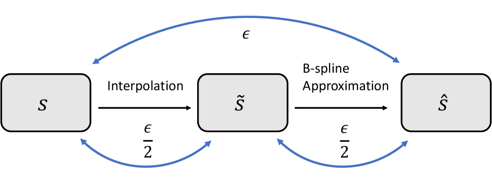
For the two surfaces and , we first find two continuous functions and for approximation. Specifically, and are interpolations of sampled data on and with grids along -th dimension, . Since Assumption 4.4 holds, from Lemma 4.2 we know that there exist , and control points and of dimension such that , . We also know that the optimal control points are obtained by solving the following least square (LS) problem to fit the sampled data on and .
| (53) | |||
where and are the sets of all sampled data on and . And we can write the LS problem into the matrix form as follow.
| (54) | |||
where and as . Here as . Then by results from the LS problems with perturbation (Wei, 1989), we know that the difference of the LS solutions of the two problems in equation 54 is bounded by
| (55) |
where as .
Since and are continuous functions defined on bounded domain, we know that both functions are Lipschitz. We denote the larger Lipschitz constants of the two functions along dimension , i.e., ,
| (56) | |||
Then we know
| (57) | |||
since and are the interpolations of sampled data on and with grids along -th dimension. We know that and when for all . Thus, we can find such that , . Then by the triangle inequality we have
| (58) | |||
∎
A.4 Remarks on Theorem 4.6
A.5 Proof of Theorem 4.7
Proof.
(Theorem 4.7) For any and , from Lemma 4.2 we know that there is and the control points realization such that for any , where is the B-spline approximation defined in equation 11 with the control points tensor . Then, from Theorem 4.6 we know that there is a DBSN configuration and corresponding parameters such that for any . Since B-spline functions of any order are continuous and Lipschitz (Prautzsch, 2002; Kunoth et al., 2018), we know that for some Lipschitz related constant . Then by triangle inequality of the norm, we have
| (59) |
For any we can find and such that to bound the norm. ∎
Appendix B Additional Theoretical Results
B.1 Convex Hull property of B-splines
Considering a one-dimensional B-spline of the form as equation 8, where , we have
| (60) |
where
This property is inherent to the Bernstein polynomials used to generate Bézier curves. Specifically, the Bézier curve is a subtype of the B-spline, and it is also possible to transform Bézier curves into B-splines and vice versa (Prautzsch, 2002).
This property also holds in the multidimensional case when the B-spline is represented by a tensor product of the B-spline basis functions in equation 11 (Prautzsch, 2002):
| (61) |
where
This property offers a practical tool for verifying the reliability of the results produced by the trained learning scheme. In the case of learning recovery probabilities, the approximated solution should provide values between and . Since the number of control points is finite, a robust and reliable solution occurs if all generated control points are within the range , i.e.,
B.2 Generalization Error Analysis
In this section, we provide justification of generalization errors of the proposed PI-DBSN framework. Specifically, given a well-trained coefficient network, we bound the prediction error of PI-DBSN on families of PDEs. Such error bounds have been studied for fixed PDEs in the context of PINNs in Mishra & Molinaro (2023); De Ryck & Mishra (2022).
We start by giving a lemma on PI-DBSN generalization error for fixed PDEs. From Section 4 we know that PI-DBSNs are universal approximators of PDEs. From Section 3 we know that the physics loss is imposed over the domain of interest. Given this, we have the following lemma on the generalization error of PI-DBSN for fixed parameters, adapted from Theorem 6 in Wang & Nakahira (2023).
Lemma B.1.
For any fixed PDE parameters and , suppose that is a bounded domain, is the solution to the PDE of interest, defines the PDE, and is the boundary condition. Let denote a PI-DBSN parameterized by and the solution predicted by PI-DBSN. If the following conditions holds:
-
1.
, where is uniformly sampled from .
-
2.
, where is uniformly sampled from .
-
3.
, , are Lipschitz continuous on .
Then the error of over is bounded by
| (62) |
where is a constant depending on , and , and
| (63) | ||||
with being the regularity of , is the Lebesgue measure of a set and is the Gamma function.
We then make the following assumption about the Lipschitzness of the coefficient network and the training scheme of PI-DBSN.
Assumption B.2.
In the PI-DBSN framework, the output of the coefficient network is Lipschitz with respect to its inputs. Specifically, given the coefficient network , such that , and such that , we have , for some constant .
Assumption B.3.
The training of PI-DBSN is on a finite subset of and for and , respectively. Assume that the maximum interval between the samples in and is and , and , each fully covers and , i.e., and , there exists and such that , .
Assumption B.2 holds in practice as neural networks are usually finite compositions of Lipschitz functions, and its Lipschitz constant can be estimated efficiently (Fazlyab et al., 2019). Assumption B.3 can be easily achieved since one can sample PDE parameters and with equispaced intervals in and for training.
We then have the following theorem to bound the generalization error for PI-DBSN on the family of PDEs.
Theorem B.4.
Assume Assumption 4.3, Assumption B.2 and Assumption B.3 hold. For any varying PDE parameters and with and bounded, suppose that the domain of the PDE is bounded, is the solution, defines the PDE, and is the boundary condition. Let denote a PI-DBSN parameterized by and the solution predicted by PI-DBSN. If the following conditions holds:
-
1.
, where is uniformly sampled from , for all and .
-
2.
, where is uniformly sampled from , for all and .
-
3.
, , are Lipschitz continuous on , for all and .
Then for any and , the prediction error of over is bounded by
| (64) |
where is a constant depending on parameter sets , , domain functions , , and the PDE , is some Lipschitz constant, and
| (65) | ||||
with being the regularity of , is the Lebesgue measure of a set and is the Gamma function.
Proof.
The goal is to prove equation 64 holds for any and . Without loss of generality, we pick arbitrary and to evaluate the prediction error, and we denote the ground truth and PI-DBSN prediction as and , respectively. From Assumption B.3 we know that there are and such that , . Let and denote the ground truth and PI-DBSN prediction on the PDE with parameters and . Since the conditions in Theorem B.4 hold for all and , and and are taking the maximum among all , we know the following inequality holds due to Lemma B.1.
| (66) |
where is a constant depending on , and , and , are given by equation 65. Note that the domain considered is , as eventually we will bound the error in this domain. Necessary mapping of the domain is applied here and in the rest of the proof when .
Since and are bounded, and from Assumption 4.3 we know the PDE solution is continuous in and , we know the solution is Lipschitz in and . Then we have
| (67) |
for some Lipschitz constant .
Lastly, from Assumption B.2 we know that the learned control points from the coefficient network are Lipschitz in and . Since the B-spline basis functions are bounded by construction, we know that
| (68) |
for some constant .
Now, combining equation 66, equation 67 and equation 68, by triangular inequality we get
| (69) | ||||
where is a constant depending on parameter sets , , domain functions , , and the PDE , is a Lipschitz constant. Since and are arbitrarily picked in and , taking will give equation 64, which completes the proof. ∎
Appendix C Experiment Details
C.1 Training Data
Recovery Probabilities: The convection diffusion PDE defined in equation 29 and equation 30 has analytical solution
| (70) |
where is the parameter of the boundary of the set in equation 27, and is the parameter of the system dynamics in equation 26. We use numerical integration to solve equation 70 to obtain ground truth training data for the experiments.
C.2 Network Configurations
Recovery Probabilities: For PI-DBSN and PINN, we use 3-layer fully connected neural networks with ReLU activation functions. The number of neurons for each hidden layer is set to be . For PI-DeepONet, we use 3-layer fully connected neural networks with ReLU activation functions for both the branch net and the trunk net. The number of neurons for each hidden layer is set to be . All methods use Adam as the optimizer.
3D Heat Equations: We set the B-splines to have the same number of equispaced control points in each direction including time. We sample the solution of the heat equation at 21 equally spaced locations in each dimension. Thus, each time step consists of control points and each sample returns control points total. The inputs to our neural network are the values of from which it learns the control points, and subsequently the initial condition surface via direct supervised learning. This is followed by learning the control points associated with later times, () via the PI-DBSN method. Because of the natural time evolution component of this problem, we use a network with residual connections and sequentially learn each time step. The neural network has a size of about learnable parameters.
C.3 Training Configurations
All comparison experiments are run on a Linux machine with Intel i7 CPU and 16GB memory.
C.4 Evaluation Metrics
The reported mean square error (MSE) is calculated on the mesh grid of the domain of interest. Specifically, for the recovery probability experiment, the testing data is generated and the prediction is evaluated on with and . For the 3D heat equation problem, the testing evaluation is on with .
The used in evaluating data and physics losses denote absolute values.
C.5 Loss Function Values
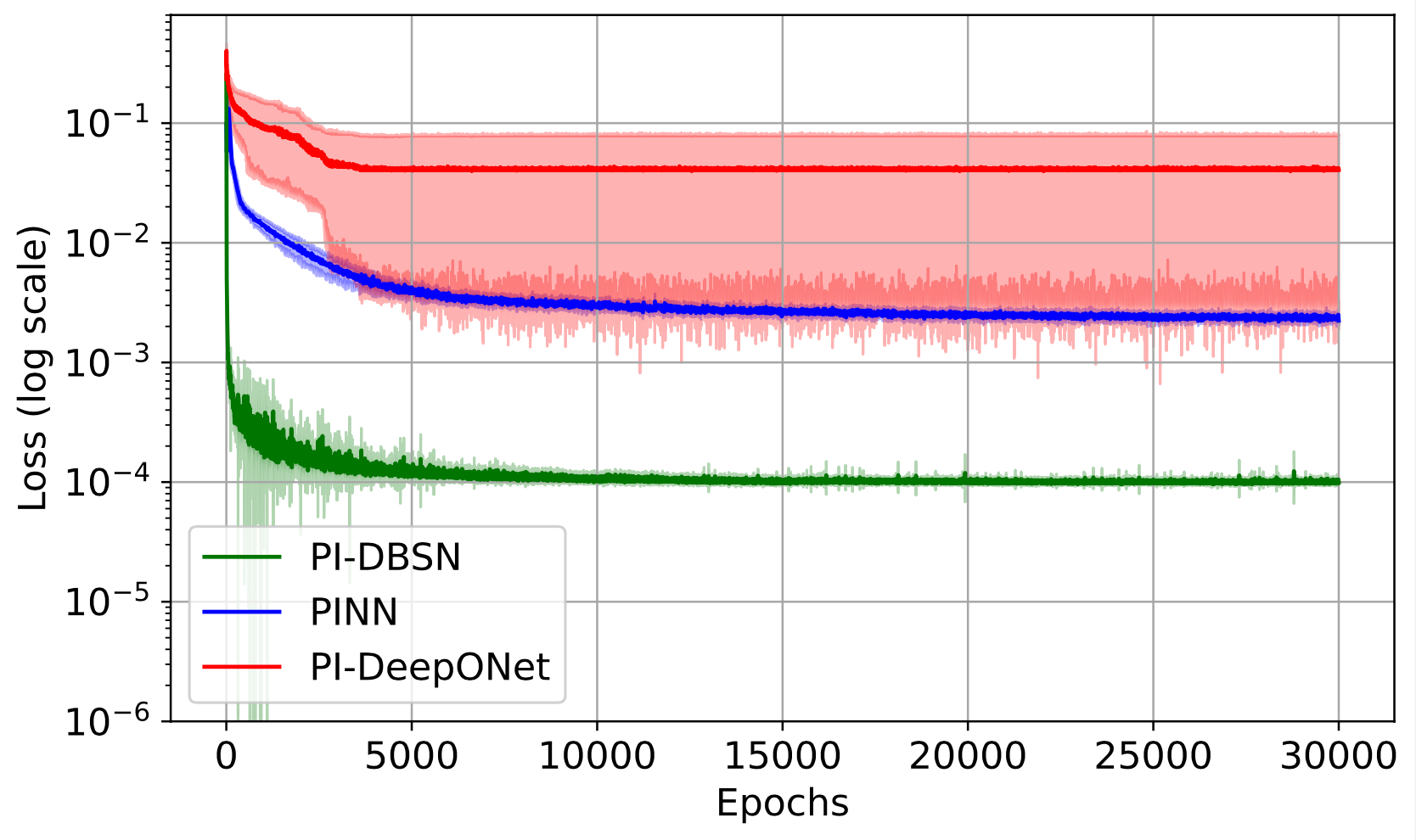
We visualize the physics loss and data loss separately for all three methods considered in section 5.1. Fig. 6 shows the physics loss and Fig. 7 shows the data loss (without ICBC losses for fair comparison with PI-DBSN). We can see that PI-DBSN achieves similar physics loss values compared with PINN, but converges much faster. Besides, PI-DBSN achieves much lower data losses under this varying parameter setting, possibly due to its efficient representation of the solution space. PI-DeepONet has high physics and data loss values in this case study.
C.6 PINN Performance on 3D Heat Equations
We report results of PINN (Raissi et al., 2019) for the 3D heat equations case study in section 5.2 for comparison. The PINN consists of 4 hidden layers with 50 neurons in each layer. We use Tanh as the activation functions. We train PINN for 30000 epochs, with physics and data loss weights . Fig. 8 visualizes the PINN prediction along different planes. The testing residual is , which is higher than the reported value () for PI-DBSN.
Appendix D Ablation Experiments
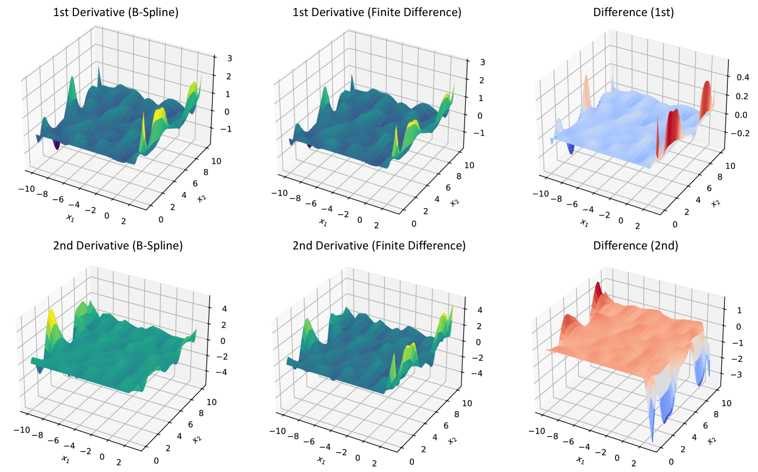
D.1 B-spline Derivatives
In this section, we show that the analytical formula in equation 15 can produce fast and accurate calculation of B-spline derivatives. Fig. 9 shows the derivatives from B-spline analytical formula and finite difference for the 2D space with the number of control point . The control points are generated randomly on the 2D space, and the derivatives are evaluated at mesh grids with . We can see that the derivatives generated from B-spline formulas match well with the ones from finite difference, except for the boundary where finite difference is not accurate due to the lack of neighboring data points.
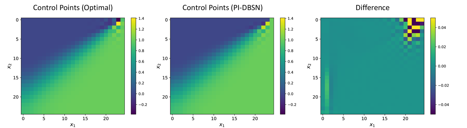
D.2 Optimality of Control Points
In this section, we show that the learned control points of PI-DBSN are near-optimal in the norm sense. For the recovery probability problem considered in section 5.1, we investigate the case for a fixed set of system and ICBC parameters and . We use the number of control points on the domain , and obtain the optimal control points in the norm sense by solving least square problem (Deng & Lin, 2014) with the ground truth data. We then compare the learned control points with and the results are visualized in Fig. 10. We can see that the learned control points are very close to the optimal control points, which validates the efficacy of PI-DBSN. The only region where the difference is relatively large is near , where the solution is not continuous and hard to characterize with this number of control points.
D.3 Experiments on GPUs
We tested the performance of PI-DBSN and the baselines on a cloud server with one A100 GPU. Note that our implementations are in PyTorch (Paszke et al., 2019), thus it naturally adapts to both CPU and GPU running configurations. The experiment settings are the same as in section 5.1. The running time of the three methods are reported in Table 3. We can see that GPU implementation accelerates training for all three methods, and PI-DBSN has the shortest running time, which is consistent with the CPU implementation results.
| Method | Computation Time (s) |
| PI-DBSN | 271 |
| PINN | 365 |
| PI-DeepONet | 429 |
D.4 Robustness and Loss Function Weights Ablations
In this section, we provide ablation experiments of the proposed PI-DBSN with different loss function configurations, and examine its robustness again noise. The setting is described in section 5.1. We first train with noiseless data and vary the data loss weight . Table 4 shows the average MSE and its standard deviation over 10 independent runs. We can see that with more weights on the data loss, the prediction MSE reduces as noiseless data help with PI-DBSN to learn the ground truth solution. We then train with injected additive zero-mean Gaussian noise with standard deviation 0.05 and vary the physics loss weight . Table 5 shows the results. It can be seen that increasing physics loss weights help PI-DBSN to learn the correct neighboring relationships despite noisy training data, which reduces prediction MSE. In general, the weight choices should depend on the quality of the data, the training configurations (e.g., learning rates, optimizer, neural network architecture).
| 1 | 2 | 3 | 4 | 5 | |
| 1 | 1 | 1 | 1 | 1 | |
| Prediction MSE () | |||||
| 1 | 1 | 1 | 1 | 1 | |
| 1 | 2 | 3 | 4 | 5 | |
| Prediction MSE () | |||||
D.5 Number of NN Layers and Parameters Ablation
In this section, we show ablation results on the number of neural network (NN) layers and parameters. We follow the experiment settings in section 5.1, and train the proposed PI-DBSN with different numbers of hidden layers, each with 10 independent runs. The number of NN parameters, the prediction MSE and its standard deviation are shown in Table 6. We can see that with 3 layers the network achieves the lowest prediction errors, while the number of layers does not have huge influence on the overall performance.
| Number of Hidden Layers | 2 | 3 | 4 | 5 |
| Number of NN parameters | 37632 | 41792 | 45952 | 50112 |
| Prediction MSE () | ||||
Appendix E Additional Experiments
In this section, we provide additional experiment results on Burgers’ equations and Advection equations, by adapting the benchmark problems in PDEBench Takamoto et al. (2022) to account for varying system and ICBC parameters.
E.1 Burgers’ Equation
We conduct additional experiments on the following Burgers’ equation.
| (71) |
where and is a changing parameter. The domain of interest is set to be , and the initial condition is
| (72) |
where is a changing parameter. We train PI-DBSN with 3-layer fully connected neural networks with ReLU activation on varying parameters and , and test on randomly selected parameters in the same domain. The B-spline basis of order is used and the number of control points along and are set to be . Note that more control points are used in this case study compared to the convection diffusion equation in section 5.1, as the solution of the Burgers’ equation has higher frequency along the ridge which requires finer control points to represent. Fig. 11 visualizes the prediction results on several random parameter settings. The average MSE across 20 test cases is . This error rate is comparable to the Fourier neural operators as reported in Figure 3 in Li et al. (2020).
E.2 Advection Equation
We consider the following advection equation
| (73) |
where is a changing parameter. The domain of interest is set to be , and the initial condition is given by
| (74) |
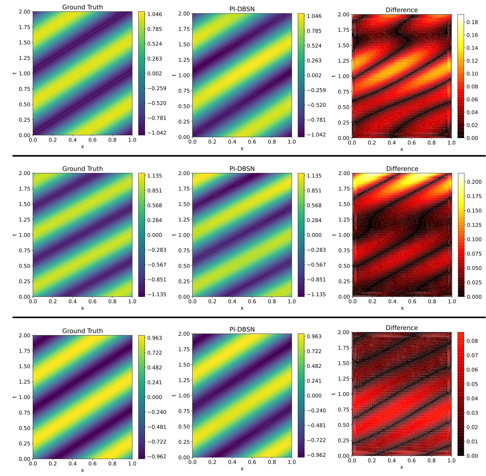
where , , and is a changing parameter. We train PI-DBSN with 3-layer fully connected neural networks with ReLU activation on varying parameters and , and test on randomly selected parameters in the same domain. The B-spline basis of order is used and the number of control points along and are set to be . Note that more control points are used in this case study to represent the high frequency solution. Fig. 12 visualizes the prediction results on several random parameter settings. The average MSE across 30 test cases is .
Appendix F Extension to Non-Rectangular Domains
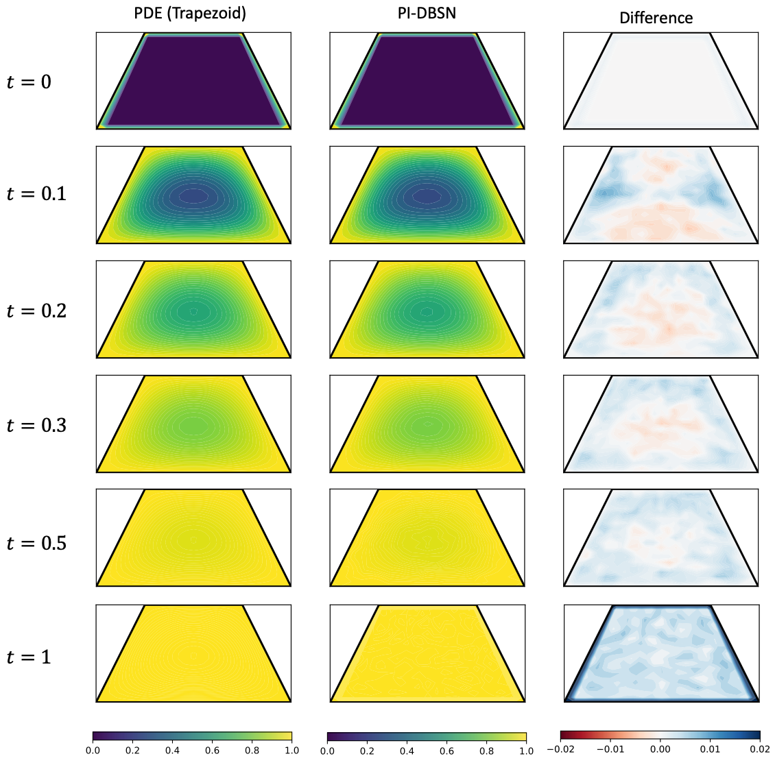
In the main text, we consider domain in . In this section, we show how the proposed method can be generalized to non-rectangular domains. The idea is that, given a non-rectangular (state) domain of interest that defines the PDE, we transform the PDE to a rectangular domain , and learn the transformed PDE on with the proposed PI-DBSN. With this mapping, one can back-propagate data loss and physics loss to train PI-DBSN. Once the network is trained, one can predict the solution of the transformed PDE on first, then tranform it back to the target domain . Below we show an example.
We wish to estimate the probability that a driftless Brownian motion, starting at a point in a trapezoidal domain
| (75) |
will hit (i.e., exit) the domain within a given time horizon with . Equivalently, if we denote by
| (76) |
then we wish to compute for all starting positions and .
We know that the exit probability is the solution of the following diffusion equation
| (77) |
where is a unknown parameter. And the ICBCs are
| (78) | ||||
We define the square mapped domain as
| (79) |
and we can find the mapping from the target domain to this mapped domain as
| (80) |
which maps the left boundary of to the left edge of and the right boundary to the right edge , while preserving . The inverse mapping is then given by
| (81) |
Note that the mapped domain can be readily handled by PI-DBSN. We then derive the transformed PDE on the mapped square domain to be
| (82) |
where
| (83) |
The corresponding ICBCs are
| (84) | ||||
For efficient evaluation of the physics loss, we approximate equation 82 with the following anisotropic but cross‐term-free PDE
| (85) |
We then generate 50 sample solutions of equation 77 with varying uniformly sampled from , and transform the solution from to via equation 80 as training data. We construct a PI-DBSN with 3-layer neural network with ReLU activation functions and 64 hidden neurons each layer. The number of control points are and . The order of B-spline is set to be . We train the coefficient network with Adam optimizer with initial learning rate for 3000 epoch. Note that the physics loss enforces equation 85 on , which is the domain for PI-DBSN training. We use and as the loss weights for training. We use a smaller weight for physics loss since the physics model is approximate. We then test the prediction results on unseen randomly sampled from . Fig. 13 visualizes the PDE solution on the trapezoid over time, the PI-DBSN prediction after domain transformation, and their difference, for one test case. It can be seen that even on this unseen parameter, the PI-DBSN prediction matches with the ground truth solution, over the entire time horizon. The MSE for prediction is , and the mean absolute error is , for 10 random testing trials.