remarkRemark \newsiamremarkhypothesisHypothesis \newsiamremarkassumptionAssumption \newsiamthmclaimClaim \headersPhase-field model with interfacial reaction and deformationZhaoyang Wang, Huaxiong Huang, Ping Lin and Shixin Xu
A thermodynamically consistent phase-field model for mass transport with interfacial reaction and deformation††thanks: Submitted to the editors April 5, 2025. \fundingZ. Wang is partially supported by the China Postdoctoral Science Foundation under grant 2024M760239. H. Huang is partially supported by the National Natural Science Foundation of China 12231004. P. Lin is partially supported by the National Natural Science Foundation of China 12371388, 11861131004 and 11771040. S. Xu is partially supported by the National Natural Science Foundation of China 12071190.
Abstract
In this paper, a thermodynamically consistent phase-field model is proposed to describe the mass transport and reaction processes of multiple species in a fluid. A key feature of this model is that reactions between different species occur only at the interface, and may induce deformation of the interface. For the governing equations derived based on the energy variational method, we propose a structure-preserving numerical scheme that satisfies the mass conservation and energy dissipation laws at the discrete level. Furthermore, we carry out a rigorous error analysis of the time-discrete scheme for a simplified case. A series of numerical experiments are conducted to validate the effectiveness of the model as well as the accuracy and stability of the scheme. In particular, we simulate microvessels with straight and bifurcated structures to illustrate the risk of microaneurysm formation.
keywords:
Phase-field model, Reaction diffusion, Interface deformations, Numerical method, Microaneurysm76T99, 65M60, 65N12
1 Introduction
Transmembrane transport of substances and reactions occurring at the membrane (interface) are common processes in both industrial and biological systems. In chemical engineering, membrane separation technologies [26] and transmembrane transport [1] in reaction processes are essential components of many industrial operations. The transmembrane transport of species and the reactions occurring at the vessel wall [2] in the human body are closely associated with health. A typical example is the formation of retinal microaneurysms [10]. Under hyperglycemic conditions, structural proteins adhered to the vascular wall react with glucose, leading to the formation of advanced glycation end-products (AGEs). The accumulation of AGEs induces vascular wall stiffening and loss of elasticity, eventually contributing to the formation of retinal microaneurysms [33].
These processes, characterized by the dynamic interaction of mass transport, interfacial reactions, and the potentially resulting mechanical deformations in fluid environments, present significant challenges for mathematical modeling and numerical simulation. Conventional reaction-diffusion models usually consider reactions to occur uniformly within a domain, and rarely pay attention to the reaction characteristics and topological changes at the interface or membrane. However, changes in the shape of the solid interface caused by the reaction may affect the dynamic behavior of other coupled fields [36]. For such fluid-structure interaction (FSI) problems, various methods have been developed, including the level set method [17, 30], the immerse boundary method [18], the front-tracking method [29, 28], and the phase-field (diffuse-interface) method [5, 8].
In particular, the phase-field method describes the membrane as a thin diffusive layer, which serves as an interface separating two incompressible fluids. The interface can be represented by the zero level-set of an order parameter. This parameter takes the values of and , corresponding to the bulk fluids inside and outside the interface, respectively, thus eliminating the need to explicitly track the interface position. Due to its ability to easily deal with the evolution of the interface over time, the phase-field method has been successfully applied to various interface deformation problems induced by fluid dynamics, such as vesicle motion [25], tumor growth [16], and moving contact line dynamics [37]. Recently, the phase-field approach has been employed to model transmembrane transport processes. Qin et al. [19] proposed a thermodynamically consistent phase-field model to describe mass transfer across the permeable moving interface, where the diffusion flux across the membrane is affected by the conductivity and concentration difference on each side. A multi-component solute diffusion model was developed in [13], which involves the crossing influences between different solutes. To the best of our knowledge, there is no work that considers reactions occurring on the membrane that cause its deformation during mass transport, despite this being quite common in the field of biology.
In this paper, we first derive a thermodynamically consistent phase-field model, which incorporates mass transport, interfacial reactions and the associated interface deformation under flow conditions into a unified framework. Unlike previous models (e.g., surfactant models [14, 35]) of interface and substances interactions, our model explicitly incorporates reactions confined to the interface that drive morphological changes. By defining energy and dissipation functionals based on the physical problem considered, and combining them with the kinematic conservation laws, we use the energy variational method to derive this model that satisfies the mass conservation and energy dissipation laws. Furthermore, we carefully design an efficient structure-preserving numerical scheme for the proposed nonlinear system, ensuring that it maintains mass conservation and energy dissipation laws at the discrete level. Given the scarcity of numerical analysis work on such problems, for the simplified case of the model, which consists of a coupled system of the Cahn-Hilliard-Navier-Stokes equations and the reaction-diffusion equation, we establish rigorous error estimates for the time-discrete scheme in for the velocity, for the pressure, for the phase function and for the concentration.
To demonstrate the practical application of the proposed model, we simulate the formation of microaneurysms in a straight vessel and further illustrate the risk of microaneurysm formation in a bifurcated vessel. We would like to point out that this work provides a theoretical and numerical framework for studying FSI problems affected by interfacial reactions and deformations, which can be easily applied to study other fluid-related interfacial dynamics problems, such as atherosclerotic plaque growth [32] and high-temperature corrosion of metals [12].
Outline
The rest of this manuscript is organized as follows. In Section 2, we introduce the energy functionals and derive the phase-field model with reactions at the interface. The mass conservation and energy dissipation laws of the model are given. In Section 3, we construct a time-discrete scheme and the corresponding fully discrete finite element scheme, and prove their mass conservation and energy stability. In Section 4, we carry out error estimates for the time-discrete scheme. Numerical results are presented in Section 5 to validate the proposed model and numerical method. The simulation of a microaneurysm is shown to demonstrate the practical application of the model. Some conclusions and remarks are given in final Section 6.
Notation
For domain and , we use the standard notation for the Banach space and the Sobolev space or . The symbol indicates the standard scalar product in . Throughout this paper, the letter denotes a generic positive constant, with or without subscript, its value may change from one line of an estimate to the next. We will write the dependence of the constant on parameters explicitly if it is essential.
2 Phase-field model with reactions at the interface
In this section, we use the energy variational method to derive a thermodynamically consistent phase-field model with reactions at the phase interface in incompressible fluids.
2.1 Model derivation
Let the problem domain be with boundary . We use as the phase-field label function, where represents one phase, represents the other phase, and denotes the interface or membrane existing between the two phases.
We assume that there are three species , and in , where can be distributed throughout the entire domain and undergo transmembrane transport, while and are confined to the interface. A reaction only occurs at the interface, where , and are stoichiometric coefficients and satisfy the conservation relation . Let denote the concentration of each species, and define as the net reaction rate function.
We start with the model derivation based on the incompressibility condition of the fluids and the mass conservation relations:
| (1a) | |||
| (1b) | |||
| (1c) | |||
| (1d) | |||
| (1e) | |||
Here, is the density of the fluid, u is the fluid velocity, is the material derivative, and j is the mass flux that will be determined later. and are stresses induced by the viscosity of the fluid and by phase interface, respectively. For variables , , , , , , , the homogeneous Neumann boundary conditions are used. For fluid velocity u, we use the no-slip boundary condition.
We define kinetic energy , phase mixing energy , entropy energy of , and mixing energies and of and in the domain as
| (2) |
where is the mixing energy density function related to the concentration of generated , and its variation implies a change in interfacial tension and may cause interface deformation. is the double well potential, is the reference concentration, is the thickness of the interface. is the energy scale in thermodynamics, and the unit is J/mol.
We would like to note that in order to ensure and only exist at the interface, local coupling terms and are added to and , inspired by the idea of constructing a surfactant model [6]. The role of terms and is to penalize the free and in the bulk phase with the penalty parameter . and enhance the adhesion of and to the interface with the parameter .
For the total energy , we can define the chemical potentials:
| (3) |
| (4) |
| (5) |
| (6) |
The dissipation functional of the system consists of the dissipation due to fluid friction, mixing of two phases in bulk, mixing and reaction of species
| (7) |
where is the fluid density, is the strain rate, is the mobility rate, are diffusion coefficients. In particular, considering the restricted diffusion of across the membrane due to the potential permeability of the interface, is defined as [19]:
| (8) |
where and are the diffusion coefficients of the two phases inside and outside the interface, respectively. , where is a function that describes the membrane permeability [34].
We would like to point out that the setting of the reaction dissipation (the last term in (7)) is motivated by the linear phenomenological constitutive laws for chemical reactions (see. e.g., [3]). This form of dissipation has also been applied in the tumor growth model [9, 31].
According to the law of energy dissipation, the rate of change of total energy equals the dissipation . By taking the time derivative of each term in the energy sequentially, we obtain
| (9) |
| (10) |
where we use the fact that .
| (11) |
| (12) |
| (13) |
Summing them up gives
| (14) |
By comparing with the predefined dissipation functional (7) yield
| (15a) | |||
| (15b) | |||
| (15c) | |||
| (15d) | |||
| (15e) | |||
| (15f) | |||
| (15g) | |||
Since the reaction only occurs at the interface, the following is a proper choice of the proliferation function :
| (16) |
The proposed model can be summarized as follows:
| (17a) | |||
| (17b) | |||
| (18a) | |||
| (18b) | |||
| (19a) | |||
| (19b) | |||
| (19c) | |||
| (20a) | |||
| (20b) | |||
| (21a) | |||
| (21b) | |||
By introducing the following dimensionless quantities:
| (22) |
where are the characteristic length, velocity, time and diffusion coefficient. In addition, we can choose to define the dimensionless variable .
Let avoiding the singularity of caused by . The dimensionless equations are as follows ( is omitted for the convenience sake):
| (23a) | |||
| (23b) | |||
| (23c) | |||
| (23d) | |||
| (23e) | |||
| (23f) | |||
| (23g) | |||
| (23h) | |||
| (23i) | |||
| (23j) | |||
| (23k) | |||
with the dimensionless parameters and . We note the no-slip boundary for u and the homogeneous Neumann boundary for , , , , , , , . Here, we redefine the pressure
2.2 Mass conservation and energy law
We introduce the following theorem.
3 Structure-preserving numerical scheme
In this section, we first construct the time-discrete scheme with the first-order accuracy for the proposed phase field model, and then prove the mass conservation and energy stability for the numerical scheme. Finally, the fully discre finite element scheme is given.
Let be a positive integer and be the final time of computation. We set be the uniform time step. Let be the numerical approximation of a specific variable at .
3.1 Time-discrete scheme
Following the stabilized method proposed in [23], we assume that the potential function satisfies the condition: there exists a constant such that . We note that the double-well potential satisfies this condition by truncating it to quadratic growth outside of an interval without affecting the solution if the maximum norm of the initial condition is bounded by . It has been a common practice to deal with phase-field problems [19, 24, 15].
The first-order time-discrete scheme is constructed as follows:
| (29a) | |||
| (29b) | |||
| (30a) | |||
| (30b) | |||
| (31a) | |||
| (31b) | |||
| (31c) | |||
| (32a) | |||
| (32b) | |||
| (33a) | |||
| (33b) | |||
Here, in (30b) is the stabilization parameter. The following homogeneous boundary conditions on the boundary:
We next prove the mass conservation and energy stability for the proposed numerical scheme. The discrete energy is defined as:
| (34) |
Theorem 3.1.
The time-discrete scheme (29)-(33) satisfies the mass conservation in the sense that
| (35) |
Let , it is energy stable in the sense that the following discrete energy law holds:
| (36) |
Here, represents non-negative terms that are independent of the energy.
Proof 3.2.
Taking the inner product of (29a), (30a) and (30b) with , and , respectively, we have
| (37) |
| (38) |
where we use the identity and the expansion:
| (39) |
Taking the inner product of (31a) and (31b) with and , respectively. We thus obtain
| (40) |
where we use the following fact:
| (41) |
Similarly, we take the inner product of (32a), (32b), (33a), and (33b) with , , and , respectively, we obtain
| (42) |
and
| (43) |
The proof is completed.
Remark 3.3.
We can see that the governing system is highly nonlinear, and the constructed numerical scheme preserves the decay of the original energy. To solve the system, we use the Newton iteration method, which may increase the computational cost. The recently developed SAV approach [22, 21] may be used to design higher-order decoupled schemes for this problem, which will be considered in future work.
3.2 Fully discrete finite element scheme
The fully discrete finite element scheme is developed in this subsection. Let be a regular triangulation of with mesh size . We use to denote the space of continuous piecewise polynomials of total degree at most . Several continuous finite element spaces are introduced as follows:
| (44) |
We assume the pair of spaces satisfy the Inf-Sup condition [7]. Let
The fully-discrete numerical scheme of system (23) reads as follows: find
such that for all , there hold
| (45a) | |||
| (45b) | |||
| (45c) | |||
| (45d) | |||
| (45e) | |||
| (45f) | |||
| (45g) | |||
| (45h) | |||
| (45i) | |||
| (45j) | |||
By following the process of proving Theorem 3.1, it is straightforward to verify that the above fully discrete scheme preserves mass conservation and the energy dissipation law.
4 Error estimates
In this section, we present a rigorous error estimate for the time-discrete scheme applied to a simplified problem, which is formulated as a nonlinear system of the Cahn-Hilliard-Navier-Stokes equations coupled with a reaction-diffusion equation. The first-order discrete scheme corresponding to subsection 3.1 is as follows:
| (46a) | |||
| (46b) | |||
| (46c) | |||
| (46d) | |||
| (46e) | |||
Here, is a constant. The boundary condition of u is no-slip, and other variables follow the homogeneous Neumann boundary condtion.
Remark 4.1.
It can be seen that the above system is a simplified version of (29), and the error analysis performed is a preliminary attempt as an illustrative example.
To derive the error estimate, we first give some necessary regularity assumptions for the exact solution. {assumption} We assume that the exact solution of the system (46) satisfies the following regularity conditions:
For notational simplicity, we set , , , , . The main results are stated in the following theorem.
Theorem 4.2.
We assume that and assumption 4.1 holds. Then for the discrete scheme (46a)-(46e), there exists a positive constant independent of such that
| (47) |
where .
Proof 4.3.
The truncation form of the system (46) is as follows:
| (48a) | |||
| (48b) | |||
| (48c) | |||
| (48d) | |||
| (48e) | |||
where , , and are the truncation errors:
| (49) |
| (50) |
| (51) |
| (52) |
Taking the inner product of (53a) with and using the regularity assumption 4.1, we have
| (54) |
where is a sufficiently small positive costant.
Let . We assume that for , which will be verified later in the proof.
The last term on the right hand side of (55) can be estimated by
| (56) |
We restrict the time step to satisfy . By combining with equations (54)-(57), summing over and using the Hölder inequality, we have
| (58) |
By using the regularity assumption 4.1 and the discrete Gronwall inequality [20], we can obtain
| (59) |
We next verify the assumption . The proof below is based on mathematical induction.
For , is obvious. We assume that holds true for , we derive is also true. It can be seen from (58) that . Applying the -elliptic regularity of (53d), we have
| (60) |
Since
| (61) |
where the Sobolev embedding theorem is used. We set the time step such that , leading to .
Next, we also use induction to estimate in -norm . Let . Assuming for .
Taking the inner product of (53a) with , we obtain
| (62) |
By the regularity of the solution to the Stokes problem (see [27]), we can get
| (64) |
For , we have . For holds true for , we can see from (64) that . Therefore,
| (65) |
We complete the induction by setting .
By setting , we thus complete the proof.
5 Numerical simulations
In this section, we first perform a numerical test to verify the accuracy and stability of the scheme. Then, we present two numerical examples to illustrate the performance of the proposed model. Finally, we conducted simulations on straight and bifurcated vascular structures to investigate risks associated with microaneurysm development. Without specific needs, we set , , , , , , , , and for simulations. The mesh size is fixed .
5.1 Convergence and stability tests
In this test, we first verify the accuracy in time of the proposed scheme by refining the time step. We set the final time , the domain , , and with . The following initial conditions are used:
| (66) |
All variables along -direction are periodic. On the top and bottom boundaries, zero Neumann and no-slip boundary conditions are used for scalar variables and velocities, respectively.
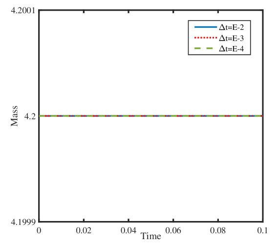
We use a finer time step to perform the test until as the reference solution. A set of decreasing time steps is used to test the convergence rate. As presented in Table 1, the results confirm the temporal accuracy of the proposed scheme. We further test the stability of the scheme. Figure 1 shows the temporal evolution of the total mass and total energy of the system under different time steps, which demonstrates the proposed scheme is mass conserved and satisfies the energy dissipation law.
| Order | Order | Order | Order | Order | ||||||
|---|---|---|---|---|---|---|---|---|---|---|
| 2.57E-2 | 8.48E-3 | 1.80E-2 | 1.44E-2 | 1.40E-2 | ||||||
| 1.65E-2 | 0.64 | 4.87E-3 | 0.80 | 1.15E-2 | 0.65 | 8.99E-3 | 0.68 | 8.86E-3 | 0.66 | |
| 9.36E-3 | 0.82 | 2.54E-3 | 0.94 | 6.54E-3 | 0.82 | 5.02E-3 | 0.84 | 5.05E-3 | 0.81 | |
| 4.68E-3 | 1.00 | 1.25E-3 | 1.02 | 3.26E-3 | 1.00 | 2.53E-3 | 0.99 | 2.54E-3 | 0.99 |
5.2 Adsorption test under shear flow
To investigate the effects of parameters and on adsorption characteristics, we set and to compare the adsorption performance of the interface on and . The initial conditions are defined to be
| (67) |
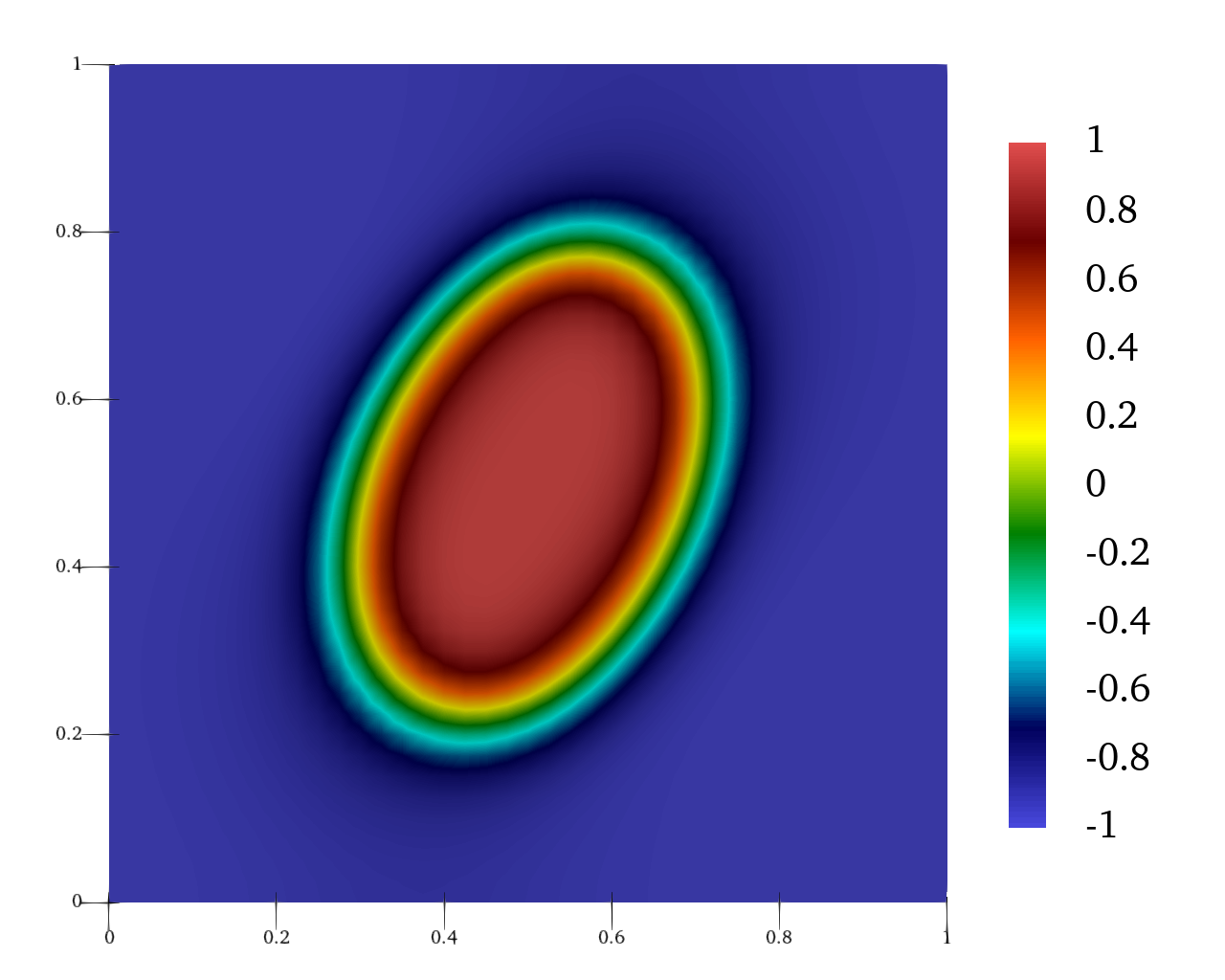
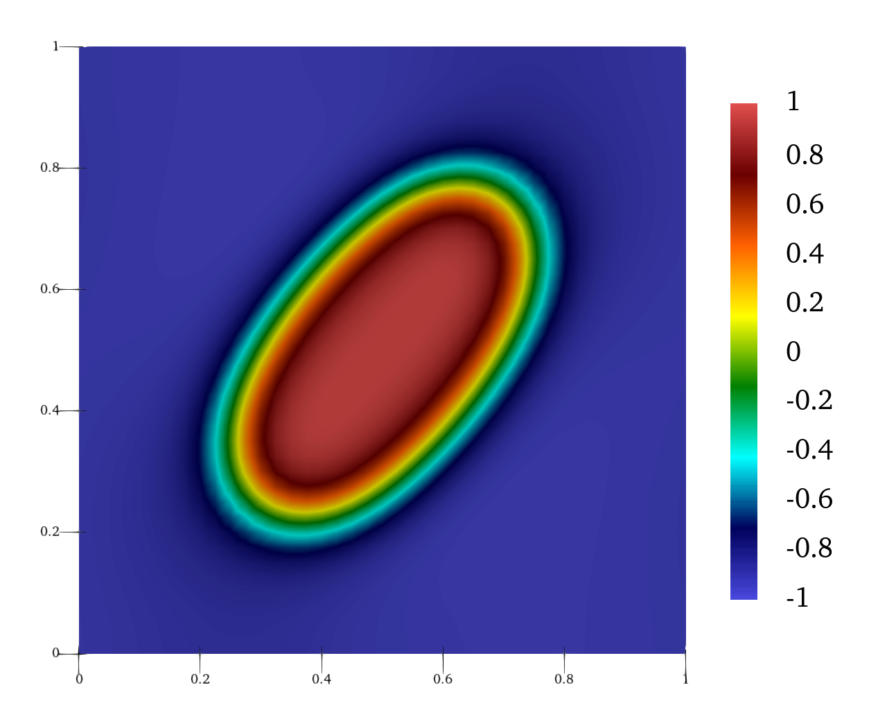
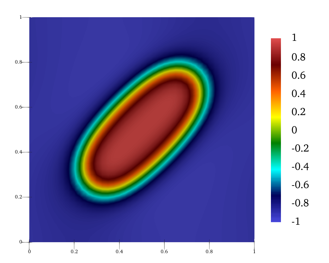
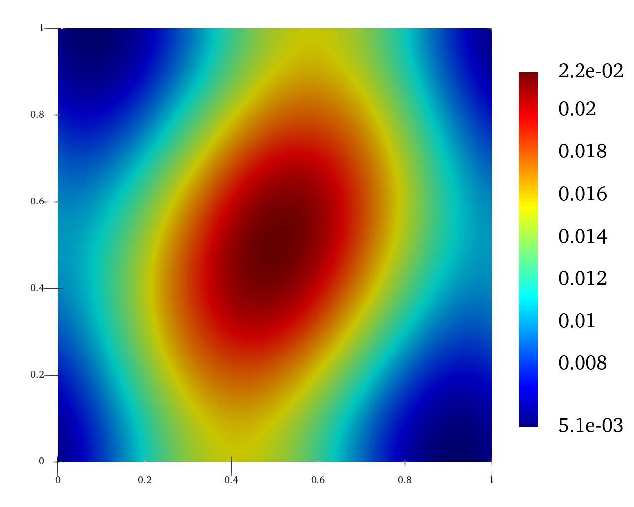
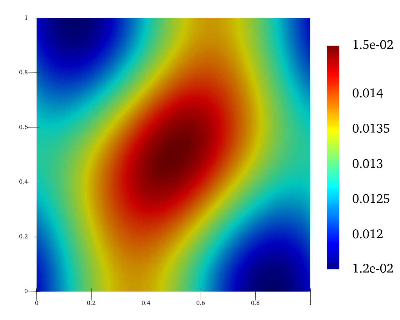
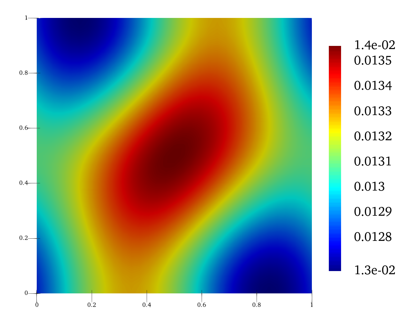
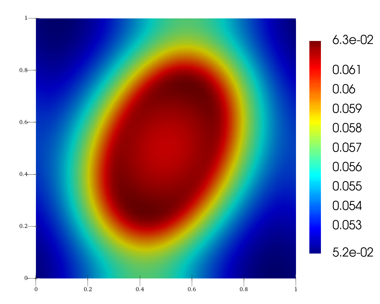
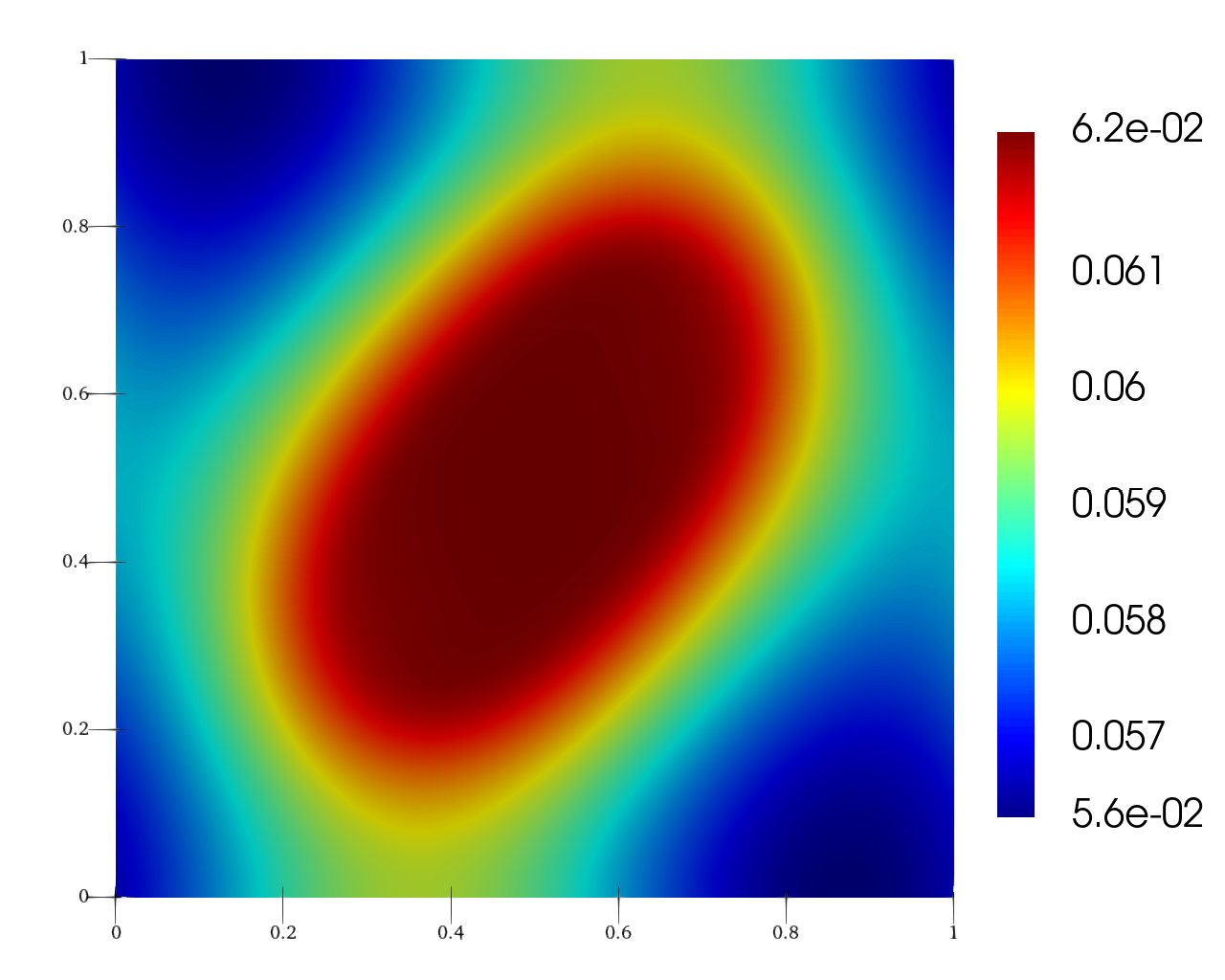
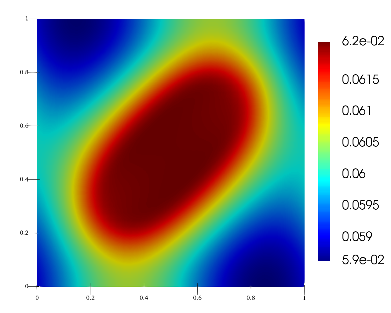
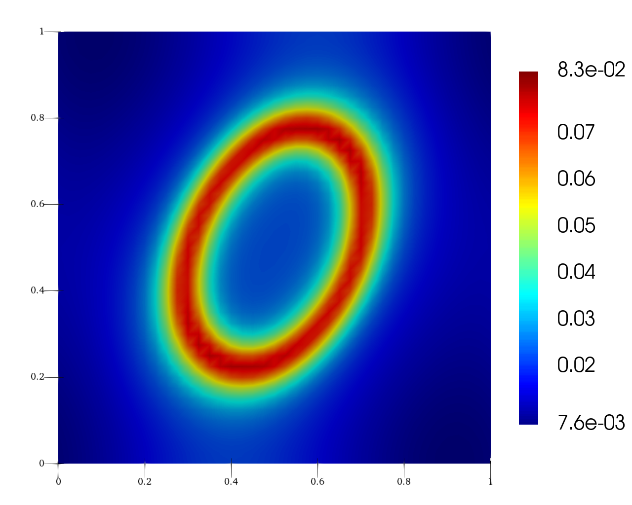
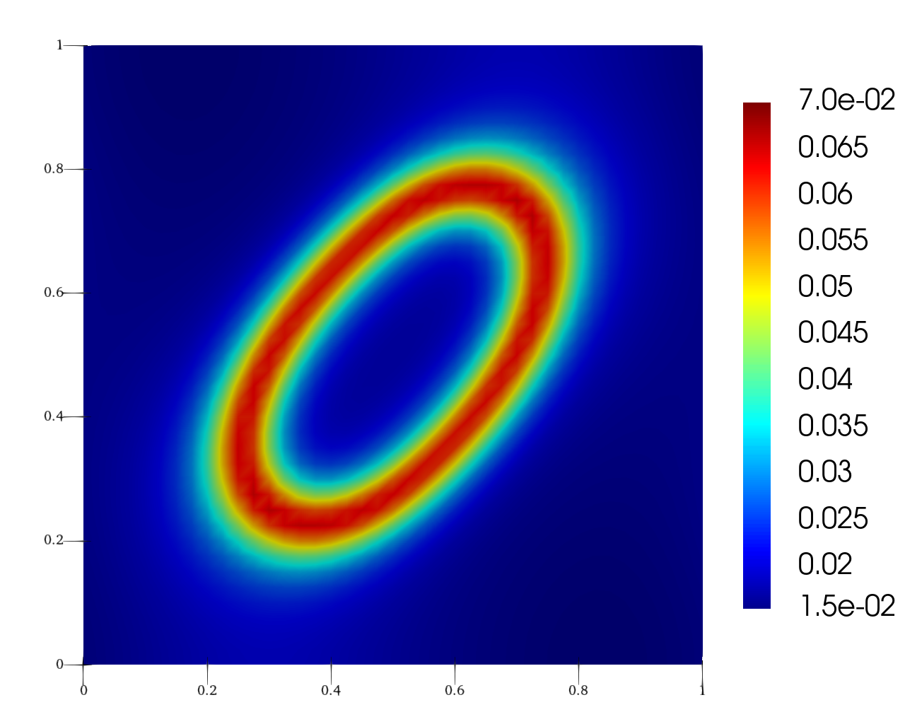
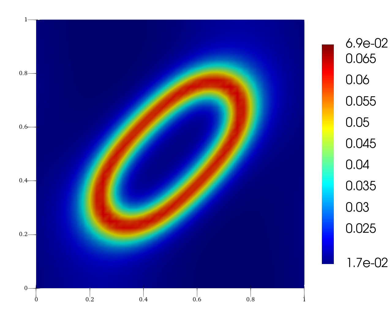
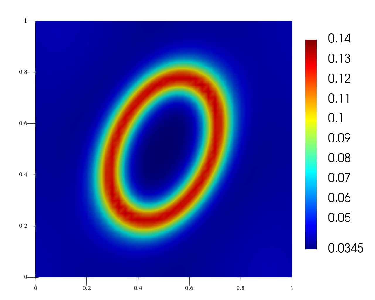
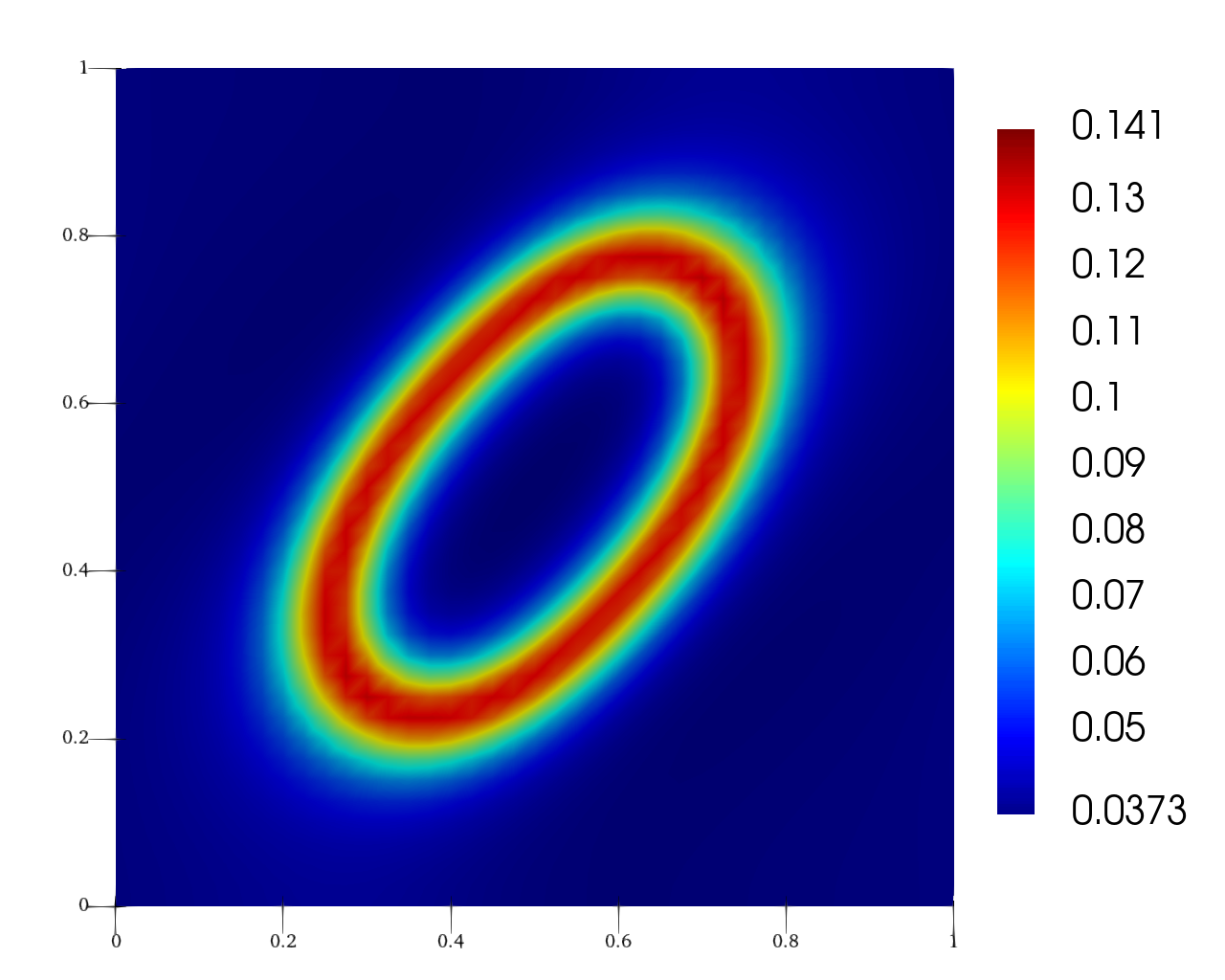
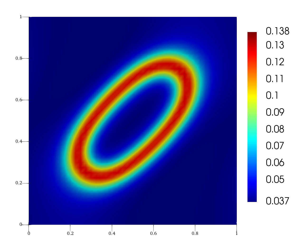
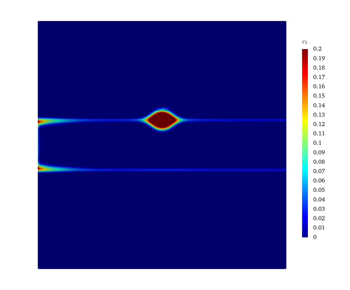
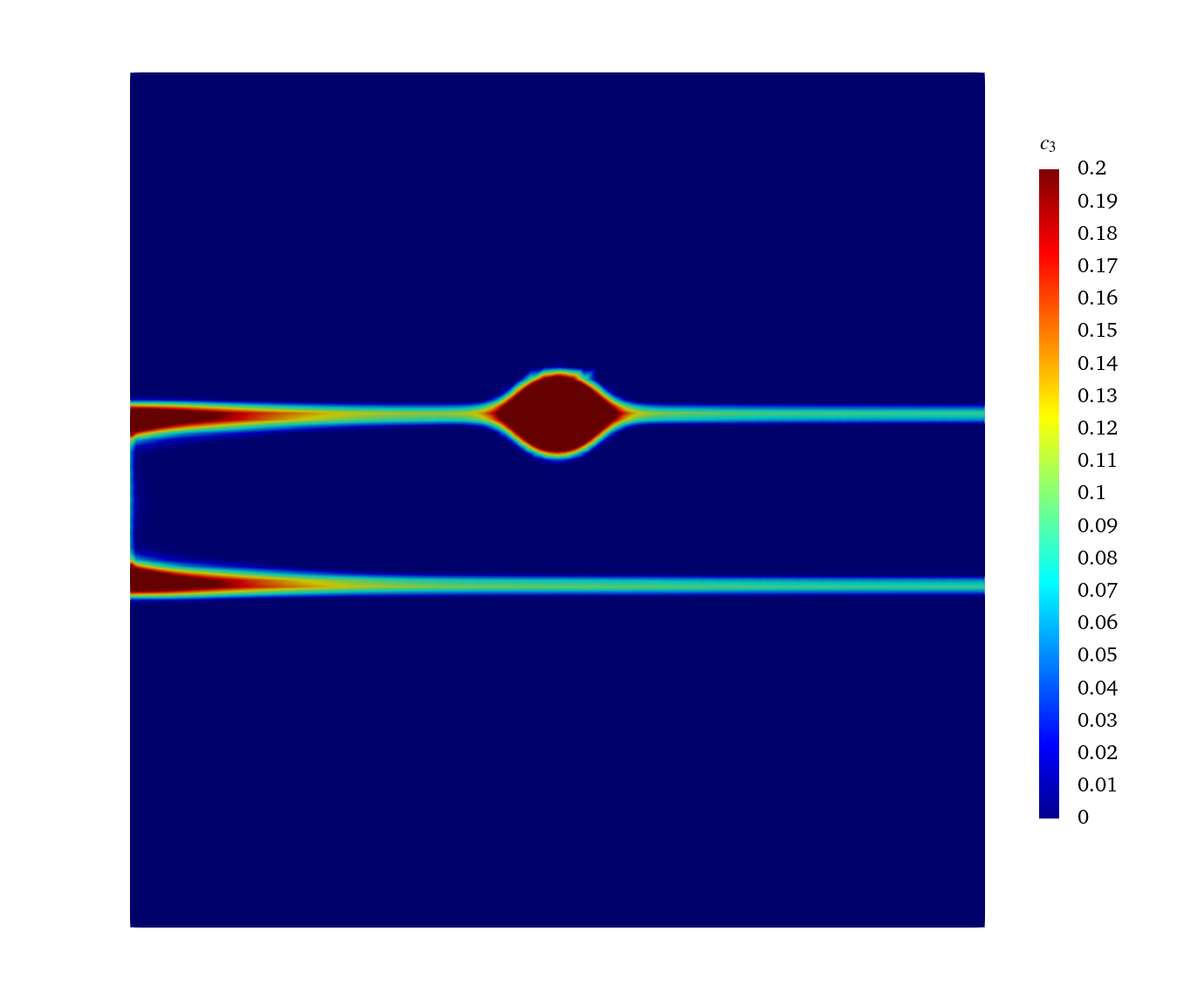
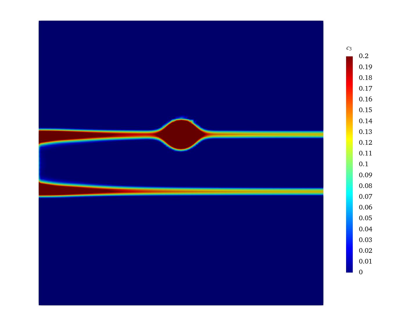
We use , and for the simulation. In the absence of adhesion effects, Figure 2 shows that the initial elliptical shape is stretched by the shear flow until a balance is achieved between the surface tension and the applied velocity. The corresponding distribution patterns of and are shown in Figure 3 and 4, both exhibiting diffusive characteristics. When , it can be seen from Figure 5 and 6 that the interface exhibits adhesion effects, with and the generated both confined to the interface.
5.3 Arterial microaneurysm
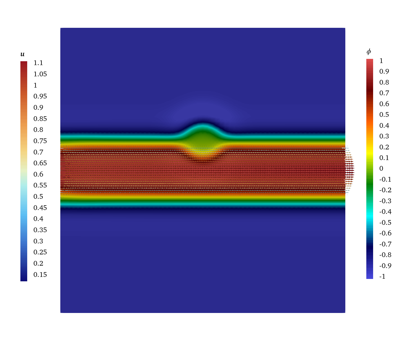
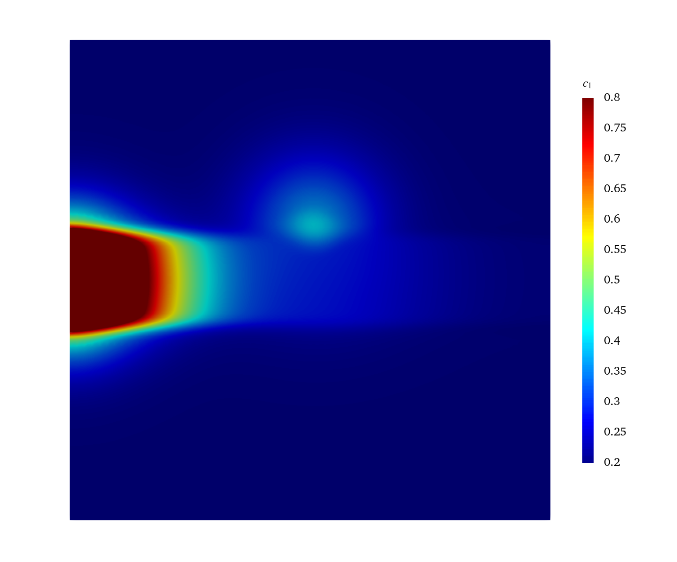
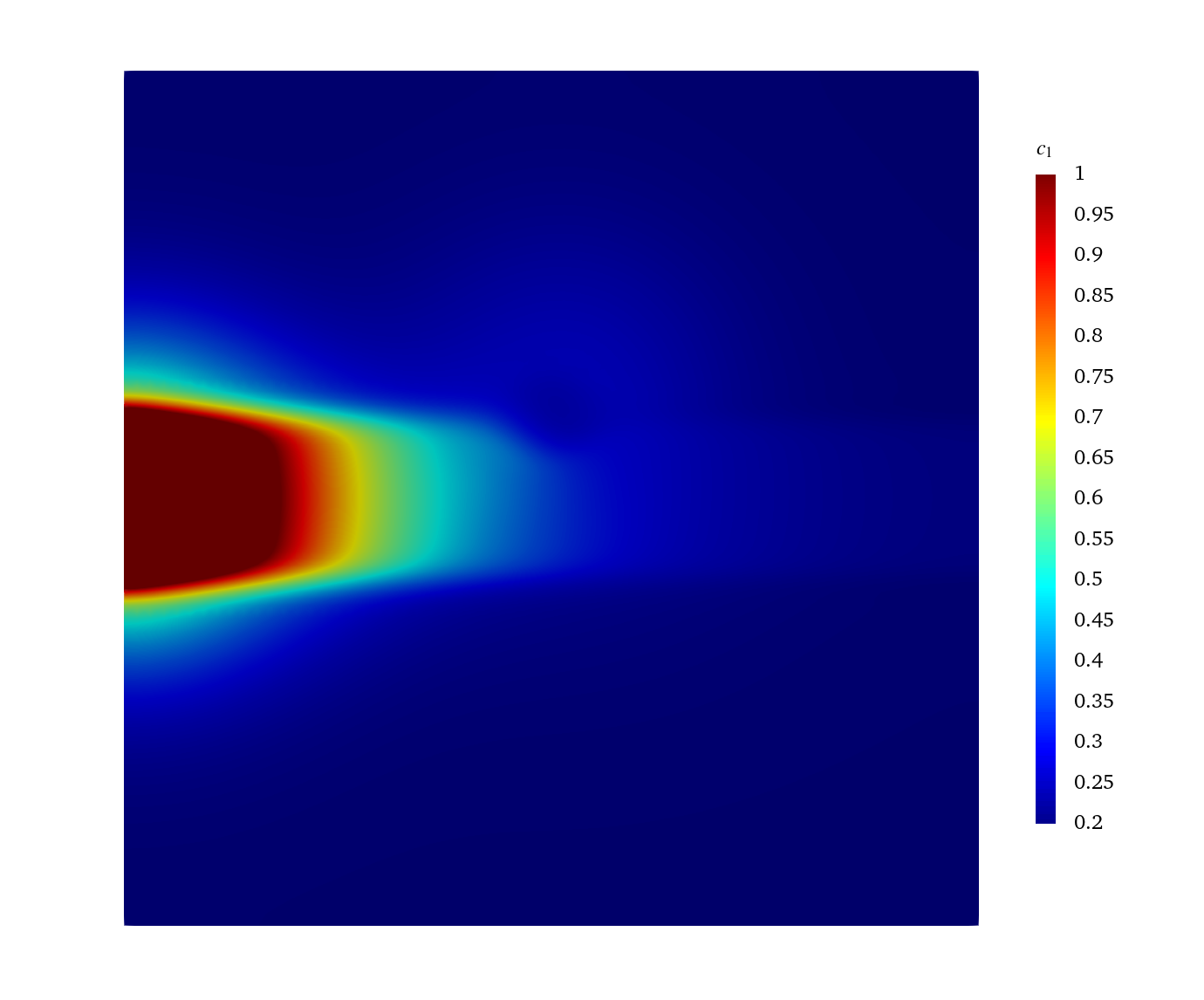
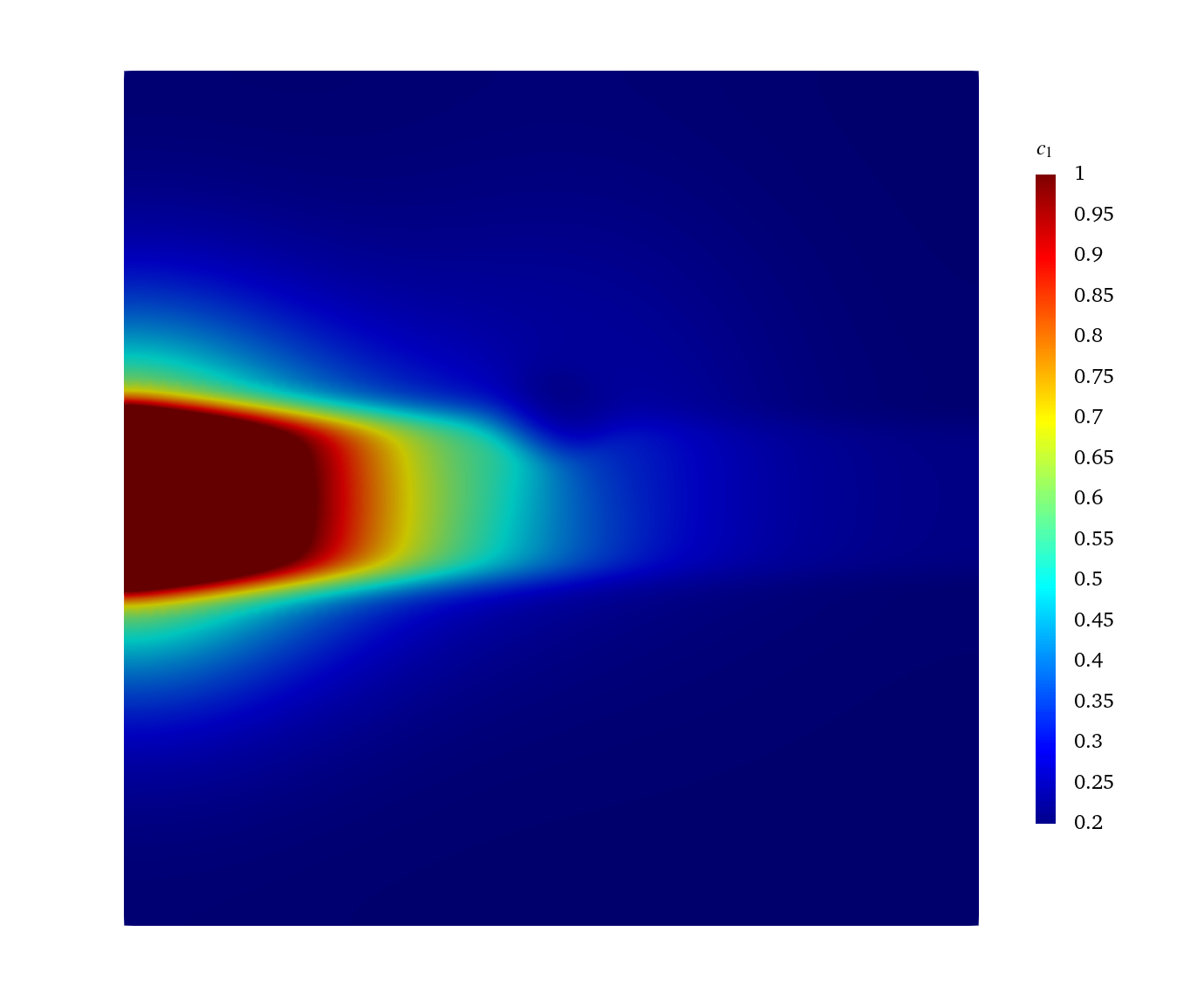
In this subsection, we apply the proposed model to the problem of microaneurysm formation. The phase-field function is regarded as the order parameter to distinguish between the two phases inside and outside the blood vessel. The diffuse interface, in which , represents the vascular wall. , and can be represented as glucose, structural proteins in the vascular wall, and advanced glycation end products (AGEs), respectively. While early glycation might be reversible, sustained AGEs accumulation leads to vascular stiffening, loss of elasticity, and structural degradation, which contribute to microaneurysm formation. In the following, we simulate microvessels with straight and bifurcated structures to illustrate the risk of microaneurysm formation.
Research has shown that AGEs disrupt endothelial junction integrity by downregulating tight junction proteins, increasing vascular permeability and promoting glucose extravasation into interstitial tissue, particularly under hyperglycemic conditions [11]. Therefore, we set in the following simulations. The settings for the other parameters are , and .
5.3.1 Straight microvessel
Straight-structured vessels are commonly observed in the microvascular system. We set the final time and the domain . The following initial and boundary conditions for and u are used:
The other boundaries of u are no-slip. For and , we set a local high concentration at the initial for the reaction to generate :
On the left boundary , the boundary condition of is set to , and on other boundaries it is the homogeneous Neumann condition.
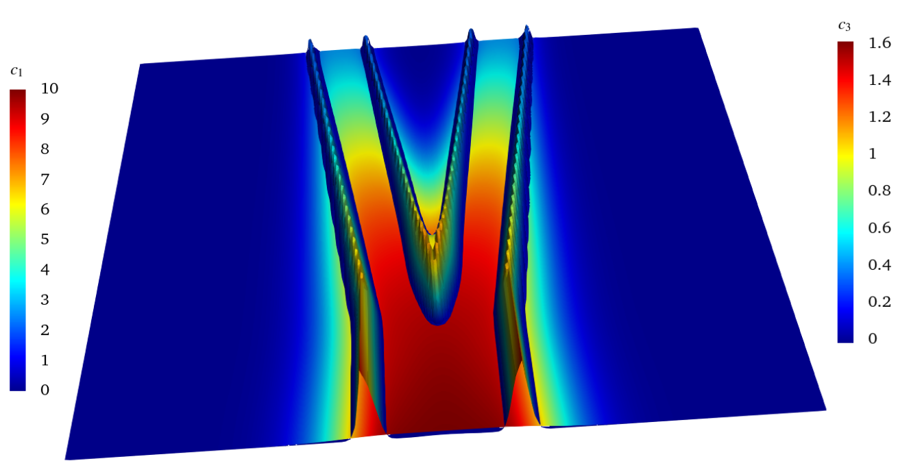
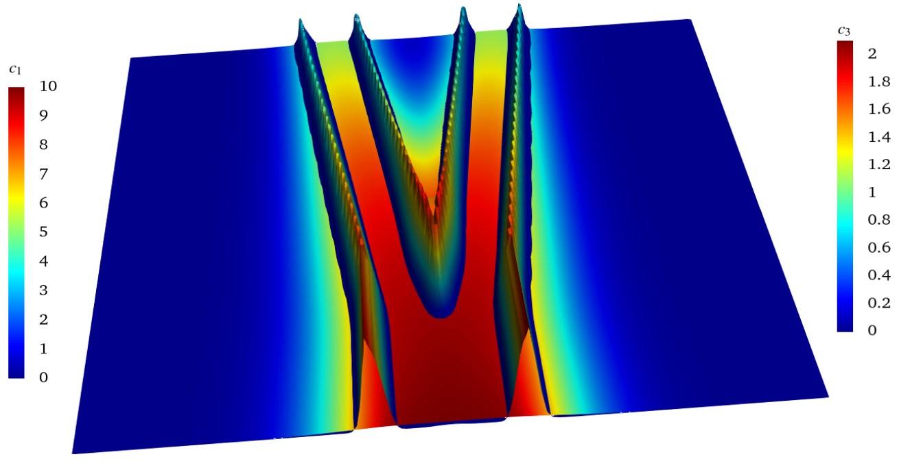
Figure 7 shows the temporal evolution of a microaneurysm within a blood vessel. We can observe that the initial stage of aneurysm formation is visible as a localized bulge, which gradually evolves into a larger size. The temporal evolution profiles of glucose and AGEs are respectively presented in Figures 8 and 9. The continuous consumption of glucose to produce AGEs correlates with the progressive aneurysm growth observed in Figure 7. Consequently, as the mixing energy density function increases, the interface tends to expand laterally to reduce the phase mixing energy of the system. In addition, it can be seen that as AGEs accumulate on the vascular wall near the inlet, glucose diffuses across the vascular wall into the interstitial fluid.


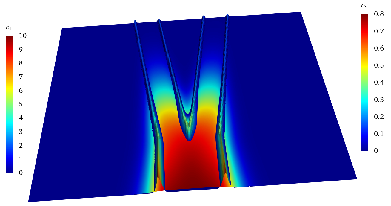
5.3.2 Bifurcated microvessel
We simulate the Y-shaped bifurcated vessel without changing the basic parameter settings to investigate the spatial distribution of AGEs. Figure 10 presents the distribution of glucose and AGEs in a bifurcated vessel structure. The influx of substantial glucose from the inlet into the vasculature, and its reaction with structural proteins on the vessel wall, results in progressive accumulation of AGEs.
Near vascular bifurcations, blood flow is prone to flow separation, generating vortex structures or stagnation zones. These hemodynamic disturbances appear to facilitate the accumulation of AGEs, which can lead to the formation of microaneurysms. We simulate vessels with larger bifurcation angles and extract the concentration of AGEs on the vascular wall at the bifurcation point for plotting. As shown in Figure 11, larger bifurcation angles are associated with higher concentrations of AGEs near the bifurcation. This phenomenon may be attributed to the hemodynamic environment, where larger bifurcation angles induce more pronounced flow separation and recirculation zones, leading to prolonged residence time, which in turn facilitates the glycation reaction.
6 Conclusions and remarks
In this paper, we develop a thermodynamically consistent phase-field model to describe mass transport, interfacial reactions, and deformation in fluid environments. The proposed model satisfies both mass conservation and energy dissipation laws. A structure-preserving numerical scheme is designed and a rigorous error analysis is performed for a simplified case. Several numerical examples verify the effectiveness of the model and the numerical method. Numerical simulations of microaneurysm formation in straight and bifurcated vessels reveal critical insights into the role of hemodynamics and AGEs accumulation.
It should be noted that the model framework proposed in this paper is not only applicable to vascular pathologies, but can also be easily adapted to corrosion processes and flows containing surfactants. In addition, this model can be combined with vesicle models [4] to describe vesicle motion under vascular deformation. The development of efficient numerical methods for the model is critically important, as it can significantly enhance computational scalability for large-scale 3-D simulations.
References
- [1] G. Bernardo, T. Araújo, T. da Silva Lopes, J. Sousa, and A. Mendes, Recent advances in membrane technologies for hydrogen purification, International Journal of Hydrogen Energy, 45 (2020), pp. 7313–7338.
- [2] L. Claesson-Welsh, E. Dejana, and D. M. McDonald, Permeability of the endothelial barrier: identifying and reconciling controversies, Trends in molecular medicine, 27 (2021), pp. 314–331.
- [3] S. R. De Groot and P. Mazur, Non-equilibrium thermodynamics, Courier Corporation, 2013.
- [4] Q. Du, C. Liu, R. Ryham, and X. Wang, Energetic variational approaches in modeling vesicle and fluid interactions, Physica D: Nonlinear Phenomena, 238 (2009), pp. 923–930.
- [5] Q. Du, C. Liu, and X. Wang, A phase field approach in the numerical study of the elastic bending energy for vesicle membranes, Journal of Computational Physics, 198 (2004), pp. 450–468.
- [6] S. Engblom, M. Do-Quang, G. Amberg, and A.-K. Tornberg, On diffuse interface modeling and simulation of surfactants in two-phase fluid flow, Communications in Computational Physics, 14 (2013), pp. 879–915.
- [7] V. Girault and P.-A. Raviart, Finite element methods for Navier-Stokes equations: theory and algorithms, vol. 5, Springer Science & Business Media, 2012.
- [8] Z. Guo and P. Lin, A thermodynamically consistent phase-field model for two-phase flows with thermocapillary effects, Journal of Fluid Mechanics, 766 (2015), pp. 226–271.
- [9] A. Hawkins-Daarud, K. G. van der Zee, and J. Tinsley Oden, Numerical simulation of a thermodynamically consistent four-species tumor growth model, International journal for numerical methods in biomedical engineering, 28 (2012), pp. 3–24.
- [10] F. E. Hirai, S. E. Moss, M. D. Knudtson, B. E. Klein, and R. Klein, Retinopathy and survival in a population without diabetes: The beaver dam eye study, American journal of epidemiology, 166 (2007), pp. 724–730.
- [11] B. I. Hudson and M. E. Lippman, Targeting rage signaling in inflammatory disease, Annual review of medicine, 69 (2018), pp. 349–364.
- [12] S. Jin, H. Tian, Q. Wang, T. Ren, P. Liu, and Z. Peng, Corrosion reaction kinetics and high-temperature corrosion testing of contact element strips in ultra-high voltage bushing based on the phase-field method, IET generation, transmission & distribution, 16 (2022), pp. 2947–2958.
- [13] J. Kou, A. Salama, and X. Wang, Thermodynamically consistent phase-field modelling of activated solute transport in binary solvent fluids, Journal of Fluid Mechanics, 955 (2023), p. A41.
- [14] M. Laradji, H. Guo, M. Grant, and M. J. Zuckermann, The effect of surfactants on the dynamics of phase separation, Journal of Physics: Condensed Matter, 4 (1992), p. 6715.
- [15] X. Meng, Y. Qin, and G. Hu, The convergence analysis of a class of stabilized semi-implicit isogeometric methods for the cahn-hilliard equation, Journal of Scientific Computing, 102 (2025), pp. 1–35.
- [16] J. T. Oden, A. Hawkins, and S. Prudhomme, General diffuse-interface theories and an approach to predictive tumor growth modeling, Mathematical Models and Methods in Applied Sciences, 20 (2010), pp. 477–517.
- [17] S. Osher, R. Fedkiw, and K. Piechor, Level set methods and dynamic implicit surfaces, Appl. Mech. Rev., 57 (2004), pp. B15–B15.
- [18] C. S. Peskin, The immersed boundary method, Acta numerica, 11 (2002), pp. 479–517.
- [19] Y. Qin, H. Huang, Y. Zhu, C. Liu, and S. Xu, A phase field model for mass transport with semi-permeable interfaces, Journal of Computational Physics, 464 (2022), p. 111334.
- [20] A. Quarteroni and A. Valli, Numerical approximation of partial differential equations, vol. 23, Springer Science & Business Media, 2008.
- [21] J. Shen, J. Xu, and J. Yang, The scalar auxiliary variable (sav) approach for gradient flows, Journal of Computational Physics, 353 (2018), pp. 407–416.
- [22] , A new class of efficient and robust energy stable schemes for gradient flows, SIAM Review, 61 (2019), pp. 474–506.
- [23] J. Shen and X. Yang, Numerical approximations of allen-cahn and cahn-hilliard equations, Discrete Contin. Dyn. Syst, 28 (2010), pp. 1669–1691.
- [24] , Decoupled, energy stable schemes for phase-field models of two-phase incompressible flows, SIAM Journal on Numerical Analysis, 53 (2015), pp. 279–296.
- [25] L. Shen, Z. Xu, P. Lin, H. Huang, and S. Xu, An energy stable finite element scheme for a phase-field model of vesicle motion and deformation, SIAM Journal on Scientific Computing, 44 (2022), pp. B122–B145.
- [26] H. Strathmann, Membrane separation processes, Journal of membrane science, 9 (1981), pp. 121–189.
- [27] R. Temam, Navier–Stokes equations: theory and numerical analysis, vol. 343, American Mathematical Society, 2024.
- [28] G. Tryggvason, B. Bunner, A. Esmaeeli, D. Juric, N. Al-Rawahi, W. Tauber, J. Han, S. Nas, and Y.-J. Jan, A front-tracking method for the computations of multiphase flow, Journal of computational physics, 169 (2001), pp. 708–759.
- [29] S. O. Unverdi and G. Tryggvason, A front-tracking method for viscous, incompressible, multi-fluid flows, Journal of computational physics, 100 (1992), pp. 25–37.
- [30] M. Y. Wang, X. Wang, and D. Guo, A level set method for structural topology optimization, Computer methods in applied mechanics and engineering, 192 (2003), pp. 227–246.
- [31] Z. Wang, P. Lin, and J. Yang, Stability and error analysis of structure-preserving schemes for a diffuse-interface tumor growth model, SIAM Journal on Scientific Computing, 47 (2025), pp. B59–B86.
- [32] Z. Wang, P. Lin, and L. Zhang, A fast front-tracking approach and its analysis for a temporal multiscale flow problem with a fractional order boundary growth, SIAM Journal on Scientific Computing, 45 (2023), pp. B646–B672.
- [33] M. Wautier and J. Wautier, Advanced glycation end products and retinal vascular lesions in diabetes mellitus, Austin J. Endocrinol. Diabetes, 2 (2015), p. 1034.
- [34] S. Xu, B. Eisenberg, Z. Song, and H. Huang, Osmosis through a semi-permeable membrane: a consistent approach to interactions, arXiv preprint arXiv:1806.00646, (2018).
- [35] X. Yang and L. Ju, Linear and unconditionally energy stable schemes for the binary fluid–surfactant phase field model, Computer Methods in Applied Mechanics and Engineering, 318 (2017), pp. 1005–1029.
- [36] Y. Yang, W. Jäger, M. Neuss-Radu, and T. Richter, Mathematical modeling and simulation of the evolution of plaques in blood vessels, Journal of mathematical biology, 72 (2016), pp. 973–996.
- [37] G. Zhu, J. Kou, B. Yao, Y.-s. Wu, J. Yao, and S. Sun, Thermodynamically consistent modelling of two-phase flows with moving contact line and soluble surfactants, Journal of Fluid Mechanics, 879 (2019), pp. 327–359.