EarlyStopping: Implicit Regularization for Iterative Learning Procedures in Python

Abstract

Iterative learning procedures are ubiquitous in machine learning and modern statistics. Regularision is typically required to prevent inflating the expected loss of a procedure in later iterations via the propagation of noise inherent in the data. Significant emphasis has been placed on achieving this regularisation implicitly by stopping procedures early. The EarlyStopping-package provides a toolbox of (in-sample) sequential early stopping rules for several well-known iterative estimation procedures, such as truncated SVD, Landweber (gradient descent), conjugate gradient descent, L2-boosting and regression trees. One of the central features of the package is that the algorithms allow the specification of the true data-generating process and keep track of relevant theoretical quantities. In this paper, we detail the principles governing the implementation of the EarlyStopping-package and provide a survey of recent foundational advances in the theoretical literature. We demonstrate how to use the EarlyStopping-package to explore core features of implicit regularisation and replicate results from the literature.

Keywords: Python, early stopping, discrepancy principle, implicit regularisation

1 Introduction

Iterative learning procedures are ubiquitous in machine learning and modern statistics. They naturally arise from the fact that estimators can often be characterised as solutions to optimisation problems which have to be approximated iteratively. Additionally, in the context of high-dimensional data sets, they are instrumental in making large scale problems computationally tractable. Any individual step of an iterative procedure is typically cheap to compute, and features of the data such as smoothness or sparsity often guarantee good estimation results after only a few iterations. Consequently, such methods can still be successful in settings where closed-form estimators become prohibitively expensive or infeasible. In statistical settings, iterative procedures typically have to be regularised to prevent inflating the expected loss (risk) of the procedure in later iterations via the propagation of noise inherent in the data. Regularisation can be explicit via optimising a penalised loss as in the case of Tikhonov regularization (Engl et al., 1996) or the Lasso (Tibshirani, 1996), implemented for instance in scikit-learn, regtools, IRtools and trips-py. Alternatively, the same effect can be achieved implicitly by stopping procedures early before convergence. Based on recent advances in the statistical literature, we introduce the EarlyStopping-package implementing data-driven early stopping rules in the context of inverse problems and regression settings, which are both statistically and computationally efficient.

Essentially, implicit regularisation translates to the choice of an appropriate iteration number $\widehat{m}$ of the learning procedure. Classically, this could be regarded as a model selection problem and be addressed via cross-validation, information criteria such as AIC and BIC, or Lepski’s balancing principle. However, all the model selection criteria above require computing the full iteration path of the procedure to determine $\widehat{m}$, which is fundamentally opposed to saving computational resources by only computing as many iterations as necessary. To retain computational efficiency, early stopping procedures therefore aim to choose $\widehat{m}$ sequentially, i.e. the moment we have reached $\widehat{m}$, we stop immediately.

One common approach to choosing $\widehat{m}$ sequentially is based on splitting the observed sample into a training and a validation set. The learning procedure is then computed on the training set and stopped when its performance on the validation set drops below a certain threshold sufficiently often, see Prechelt (2002). While there are not many theoretical guarantees for sequential sample splitting, in practical application, it is often considered state of the art and is part of most major machine learning frameworks such as Keras, XGBoost, scikit-learn, lightgbm and Pytorch.

From the theoretical side of the literature, more interest has been garnered by sequential (in-sample) early stopping rules that avoid sample splitting. On the one hand, only in specific machine learning settings, users can afford to sacrifice a significant portion of the observations. On the other hand, sample splitting is unsuitable if the dataset is highly interdependent or constitutes a single observation of a complex underlying distribution, e.g., in the case of inverse problems as treated in Blanchard and Mathé (2012), Blanchard et al. (2018a, b), Stankewitz (2020), Mika and Szkutnik (2021), Jahn (2022), Hucker and Reiß (2025) or kernel learning in Celisse and Wahl (2021). Additionally, optimal early stopping may depend on quantities that cannot be estimated from a split sample such as an empirical in-sample noise level, see Stankewitz (2024), Kück et al. (2023) and Miftachov and Reiß (2025).

These stopping rules have not found their way into mainstream software libraries yet, and implementations mostly exist isolated in specialised packages, see regtools or trips-py. In particular, to our knowledge, there exists no unified library for these closely related procedures. Our EarlyStopping-package fills this gap and provides a toolbox to analyse and experiment with (in-sample) sequential early stopping rules for several well-known iterative estimation procedures, such as truncated SVD, Landweber (gradient descent), conjugate Gradient descent, L2-boosting and regression trees.

The EarlyStopping-package primarily builds on the theoretical foundations in Blanchard et al. (2018a, b), Hucker and Reiß (2025), Stankewitz (2024), Kück et al. (2023) and Miftachov and Reiß (2025). Blanchard et al. (2018a) initially analyse the estimation performance of a residual-based stopping rule (discrepancy stop) for the truncated singular value decomposition (truncated SVD) in a statistical inverse problem and provide statistical guarantees for the estimation performance. They also explore theoretical limitations of stopping rules in terms of minimax lower bounds leading to the development of an adaptive two-step procedure. As its default, this procedure uses a sequential stopping rule and guarantees optimal performance even in pathological cases via an AIC criterion applied to only the iterations up to the stopping time. An extension of the adaptation bounds for a residual-based stopping rule is provided by Blanchard et al. (2018b) for general spectral regularisation methods such as the Landweber (gradient descent) iteration. One of the computationally most efficient methods for solving systems of linear equations is the conjugate gradient (CG) algorithm. The CG algorithm depends highly non-linearly on the observations, making the theoretical analysis particularly intricate. Adaptation bounds were nevertheless achieved by Hucker and Reiß (2025) for the discrepancy stop.

For $L^{2}$-boosting via orthogonal matching pursuit, Stankewitz (2024) showed adaptivity for the discrepancy stop in high-dimensional linear models given a suitable in-sample noise estimate, which can be obtained via the scaled Lasso studied in Sun and Zhang (2012a). Kück et al. (2023) show that under sparsity assumptions, another stopping rule, the residual ratio stop, exists that does not rely on an additional noise estimator. A recent contribution by Miftachov and Reiß (2025) extends the Early Stopping paradigm to non-parametric regression using the classification and regression tree (CART) algorithm by Breiman et al. (1984). The proposed breadth-first search and best-first search early stopping algorithms for constructing a regression tree are embedded in a much broader framework of generalised projection flows of iterative regression estimators.

The EarlyStopping-package gathers the different early stopping methods from the literature above within one common framework and provides prototypical implementations of the iterative algorithms in unified class structures. One of the central features is that the classes additionally allow the specification of the true data-generating process and are therefore able to keep track of all relevant theoretical (oracle) quantities, such as explicit bias-variance decompositions or theoretical risk minimisers. For both researchers and practitioners, the EarlyStopping-package can therefore provide a common frame of reference for experimentation, since in controlled settings, the true performance of the procedure can immediately be made explicit. The EarlyStopping-package also provides a simulation wrapper class, which yields seamless (one-line) executions of Monte-Carlo simulations. In the interest of reproducible research, this allows the instant replication of simulation studies from the literature. The EarlyStopping-package is written in Python, and its code repository and documentation are available on GitHub under the following URLs:

• Repository: github.com/EarlyStop/EarlyStopping,

• Documentation: earlystop.github.io/EarlyStopping,

The paper consists of two main parts. Section 2 introduces the necessary theoretical context and provides a survey of the existing early stopping literature. Section 3 explains the implementation of the EarlyStopping-package in detail, provides examples and replicates major results from the literature. Both sections feature detailed explanations for each of the iterative estimation procedures.

2 Background on early stopping

Iterative methods have become omnipresent in machine learning and modern statistics. They naturally arise from the fact that estimators can often be characterised as solutions of optimisation problems, which have to be solved iteratively. In statistical settings, when observations are noisy, unregularised algorithms typically cannot be iterated indefinitely and have to be stopped early, i.e. before they converge. Indeed, the risk given by the expected loss at iteration $m$ of a sequence of iteratively computed estimators $(\widehat{f}^{(m)})_{m\geq 0}$ typically can be decomposed into

$$\mathcal{R}(f^{*},m)=b_{m}^{2}(f^{*})+s_{m},\qquad m\geq 0,$$ (2.1)

where $b_{m}^{2}(f^{*})$ is a squared bias or approximation error depending on the underlying truth $f^{*}$ and $s_{m}$ is a stochastic error. The mapping $m\mapsto b_{m}^{2}(f^{*})$ is usually decreasing, as later iterations reduce the approximation error of the iterative procedure, whereas $m\mapsto s_{m}$ is increasing, since it accounts for the propagation of the noise in the observations, see Figure 1.

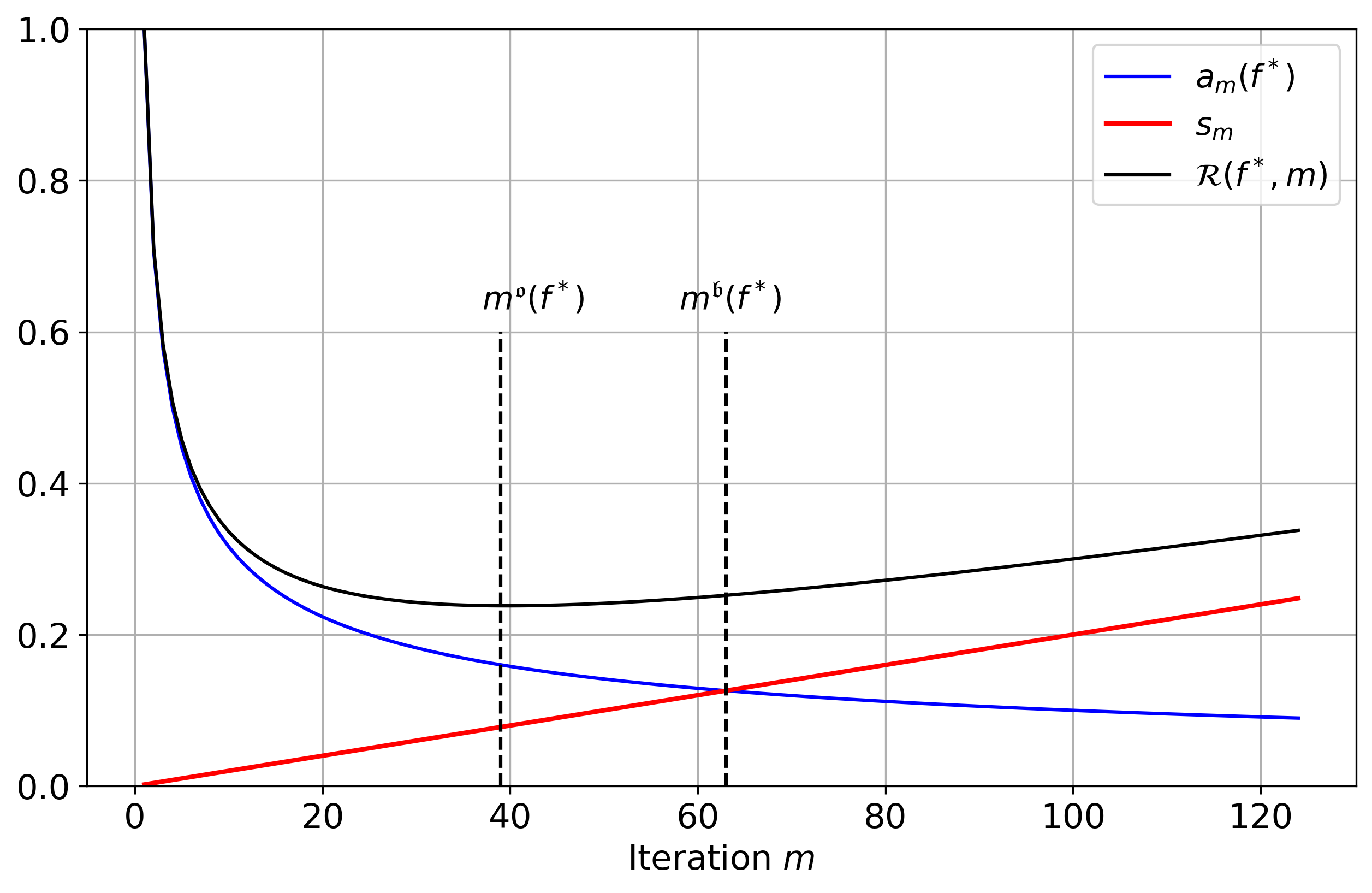
(a) Risk decomposition for a signal $f^{*}$.

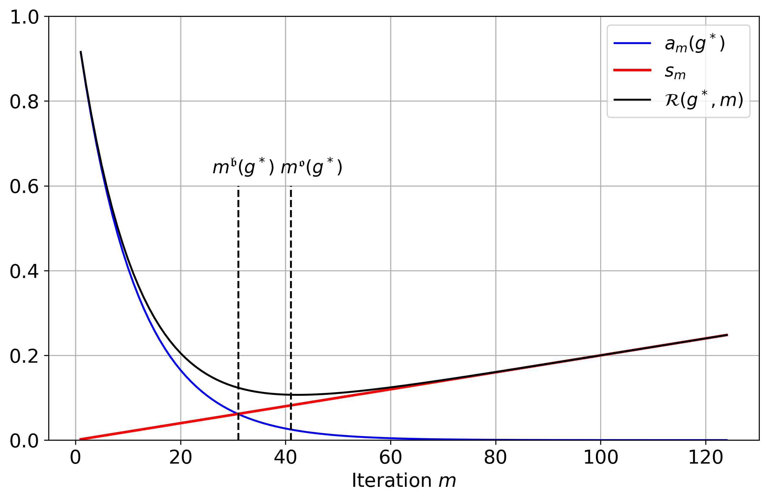
(b) Risk decomposition for a signal $g^{*}$.

Figure 1: Decomposition of the risk into approximation and stochastic error for two signals $f^{*}$ and $g^{*}$ with slowly and fast decaying squared bias respectively.

Learning $f^{*}$ amounts to (approximately) minimising the risk $\mathcal{R}(f^{*},m)$ with respect to $m\geq 0$. However, since $b_{m}^{2}(f^{*})$ depends on the unknown underlying truth $f^{*}$, this is also true for the minimiser

$$m^{\mathfrak{o}}=m^{\mathfrak{o}}(f^{*})=\operatorname*{arg\!\min}_{m\geq 0}\mathcal{R}(f^{*},m).$$ (2.2)

Consequently, the iteration number $\hat{m}$ that we ultimately choose for the procedure has to be adaptive. This means that it is chosen depending on the data in order to distinguish between both different settings in Figure 1.

In case that the full path of estimators $(\widehat{f}^{(m)})_{m\geq 0}$ is known, criteria from the model selection literature such as cross-validation Arlot and Celisse (2010), information criteria such as the Akaike information criterion (AIC) and the Bayesian information criterion (BIC) Stoica and Selen (2004) or Lepski’s balancing principle (Lepski et al., 1997) provide adaptive choices of $\hat{m}$. However, computing the full path of estimators $(\hat{f}^{(m)})_{m\geq 0}$ is fundamentally opposed to the idea of iterative estimation. In the case of the signal $g^{*}$ in Figure 1, by computing the full iteration path to then select an iteration $\hat{m}$ close to $m^{\mathfrak{o}}(g^{*})$, more than $75\%$ of computational resources would have been spent on applying a model selection criterion. Therefore, we should aim to choose $\hat{m}$ sequentially to increase the computational efficiency of the method. This means that when we have reached $\hat{m}$, we stop immediately.

Prima facie, it is not obvious that such rules should exist. For example, a sequential choice $\hat{m}$ can never directly mimic the (global) classical oracle $m^{\mathfrak{o}}$, since $\hat{m}$ does not incorporate information about $b_{m}^{2}(f^{*})$ for $m>\hat{m}$. However, it can be shown that the (sequential) balanced oracle

$$m^{\mathfrak{b}}=m^{\mathfrak{b}}(f^{*}):=\inf\{m\geq 0:b_{m}^{2}(f^{*})\leq s_{m}\}$$ (2.3)

satisfies

$$\mathcal{R}(f^{*},m^{\mathfrak{b}})\leq 2\mathcal{R}(f^{*},m^{\mathfrak{o}})+\Delta(s_{m^{\mathfrak{b}}})=2\min_{m\geq 0}\mathcal{R}(f^{*},m)+\Delta(s_{m^{\mathfrak{b}}}),$$ (2.4)

where $\Delta(s_{m}):=s_{m}-s_{m-1}$ is the discretisation error of the stochastic error at iteration $m$, see Stankewitz (2023, Lemma I.1.1). In many settings, data-driven sequential stopping rules can be constructed that mimic $m^{\mathfrak{b}}$, which is explained in more detail throughout the next section.

2.1 Early stopping for inverse problems

We consider a general finite dimensional statistical inverse problem

$$Y=Af^{*}+\delta\varepsilon,$$ (2.5)

where $A\in\mathbb{R}^{n\times p}$ is a large scale matrix, $f^{*}\in\mathbb{R}^{n}$ is an unknown coefficient signal to be recovered and $\varepsilon\in\mathbb{R}^{n}$ is standard Gaussian noise. Typically, formulations as in (2.5) stem from discretisations of potentially infinite-dimensional inverse problems, see Engl et al. (1996).

Assuming that $A$ is injective, $A^{\top}A$ is invertible and the classical least squares estimator is given by

$$\widehat{f}:=\operatorname*{arg\!\min}_{f\in\mathbb{R}^{p}}\|Y-Af\|^{2}=(A^{\top}A)^{-1}A^{\top}Y=\sum_{j=1}^{\min(n,p)}\lambda_{j}^{-1}v_{j}^{\top}Yu_{j}.$$ (2.6)

The last expression is in terms of the singular value decomposition (SVD)

$$A=V\Lambda U^{\top}=\sum_{j=1}^{\min(n,p)}\lambda_{j}v_{j}u_{j}^{\top}$$ (2.7)

of the design matrix $A$. If the inverse $(A^{\top}A)^{-1}$ does not exist, e.g. due to ill-posedness, classical regularisation methods replace $\lambda_{j}^{-1}$ on the right hand side of (2.6) with $\lambda_{j}g_{\alpha}(\lambda_{j}^{2})$, where $(g_{\alpha})_{\alpha>0}$ is an approximating family of piecewise continuous functions satisfying that for any $\lambda\in(0,\infty)$,

$$g_{\alpha}(\lambda)\to\lambda^{-1}\qquad\text{ for }\alpha\to 0.$$ (2.8)

For simplicity, we assume in the following that the inverse problem in Equation (2.5) is discretised appropriately, i.e., that $A$ is surjective and $n\leq p$. The regularised estimator is then given by

$$\widehat{f}_{\alpha}\coloneqq g_{\alpha}(A^{\top}A)A^{\top}Y=\sum_{j=1}^{n}\lambda_{j}g_{\alpha}(\lambda_{j}^{2})v_{j}^{\top}Yu_{j}.$$ (2.9)

Most of the standard regularisation methods can be represented in this way, where $\alpha\to 0$ is interpreted as a continuous idealization of the iterative computation scheme of estimators $\widehat{f}^{(m)}$ with iteration number $m\to\infty$.

Reparameterised in terms of the iteration $m$, the risk expressed as the mean integrated squared error (MISE)

$$\mathcal{R}(f^{*},m):=\mathbb{E}\|\widehat{f}^{(m)}-f^{*}\|^{2}=b_{m}^{2}(f^{*})+s_{m}$$ (2.10)

satisfies an error decomposition as in Equation (2.1). The approximation error, given by the squared bias $b_{m}^{2}(f^{*}):=\|\mathbb{E}\widehat{f}^{(m)}-f^{*}\|^{2}$, is decreasing in $m$, whereas the stochastic error, given by the variance $s_{m}:=\mathbb{E}\|\widehat{f}^{(m)}-\mathbb{E}\widehat{f}^{(m)}\|^{2}$, is increasing in $m$. Structurally, the same is true for the prediction risk

$$\mathcal{R}_{A}(f^{*},m):=\mathbb{E}\|A(\widehat{f}^{(m)}-f^{*})\|^{2}=b_{m,A}^{2}(f^{*})+s_{m,A},$$ (2.11)

which also decomposes into a decreasing approximation error $b_{m,A}^{2}(f^{*}):=\|A(\mathbb{E}\widehat{f}^{(m)}-f^{*})\|^{2}$ and an increasing noise propagation part $s_{m,A}:=\mathbb{E}\|A(\widehat{f}^{(m)}-\mathbb{E}\widehat{f}^{(m)})\|^{2}$. Following the terminology from Blanchard et al. (2018a), we call the MISE the strong risk and the prediction risk the weak risk. Given the decompositions (2.10) and (2.11), we can define strong and weak versions

$$m^{\mathfrak{b}}_{s}:=\inf\{m\geq 0:b_{m}^{2}(f^{*})\leq s_{m}\},\quad m^{\mathfrak{b}}_{w}:=\inf\{m\geq 0:b_{m,A}^{2}(f^{*})\leq s_{m,A}\},$$ (2.12)

of the balanced oracle in Equation (2.3).

In order to stop the learning procedure given by the estimators $(\widehat{f}^{(m)})_{m\geq 0}$, we focus on the discrepancy principle, which is likely the most prominent sequential iteration parameter choice rule in the inverse problem literature, see Engl et al. (1996) and Werner (2018). For a user-specified critical value $\kappa>0$, it prescribes stopping at

$$\tau^{\text{DP}}:=\min\{m\geq 0:\|Y-A\widehat{f}^{(m)}\|^{2}\leq\kappa\},$$ (2.13)

that is, the first iteration at which the remaining data misfit given by squared residuals $\|Y-A\widehat{f}^{(m)}\|^{2}$ is smaller than $\kappa$. In many settings, it can be shown that

$$\mathbb{E}\|Y-A\widehat{f}^{(m)}\|^{2}=b_{m,A}^{2}(f^{*})-s_{m,A}+n\delta^{2},$$ (2.14)

indicating that in expectation, the discrepancy stop $\tau^{\text{DP}}$ mimics the weak balanced oracle when $\kappa$ is approximately $n\delta^{2}$. We consider this in more explicit detail for the learning procedures implemented in the EarlyStopping-package.

2.1.1 Truncated SVD

The spectral cut-off (or truncated SVD) estimator emerges considering the family of functions $g_{\alpha}(\lambda)\coloneqq\lambda^{-1}\mathbf{1}_{[\alpha,\infty]}(\lambda)$ in Equation (2.8) with the discretisation $\alpha_{m}:=\lambda_{m}^{2}$, $m\geq 0$. As an iterative estimation procedure, the updating rule is given by

$$\widehat{f}^{(0)}=0,\quad\widehat{f}^{(m+1)}=\widehat{f}^{(m)}+\frac{v_{m+1}^{\top}Y}{\lambda_{m+1}}u_{m+1}=\sum_{j=1}^{m}\frac{v_{j}^{\top}Y}{\lambda_{j}}u_{j}.$$ (2.15)

For these estimators, the full SVD is usually unavailable and must be computed. The calculation of the largest singular value is less costly if deflation or locking methods are used. In the EarlyStopping-package, the singular values are computed iteratively using the power method and by sequentially removing the largest singular value from the design through

$$A_{0}=A,\quad A_{i+1}=A_{i}-\lambda_{i}u_{i}v_{i}^{\top}.$$ (2.16)

Based on this methodology, the required singular values and vectors are computed with roughly $O(mn^{2})$ multiplications. This results in a computational complexity of $O(\tau^{\text{DP}}n^{2})$ for the stopped algorithm compared to $O(n^{3})$ when considering the whole learning trajectory.

The strong risk (2.10) and weak risk (2.11) of the estimators above are given by

$$\mathcal{R}(f^{*},m) =b_{m}^{2}(f^{*})+s_{m}=\sum_{j=m+1}^{n}\langle f^{*},u_{j}\rangle^{2}+\delta^{2}\sum_{j=1}^{m}\lambda_{j}^{-2},$$ (2.17)

$$\mathcal{R}_{A}(f^{*},m) =b_{m,A}^{2}(f^{*})+s_{m,A}=\sum_{j=m+1}^{p}\lambda_{j}^{2}\langle f^{*},u_{j}\rangle^{2}+\delta^{2}m.$$

As the number $m$ of iterations increases, the number of modes contributing to the strong bias decreases, while the number of singular values contributing to the strong variance increases. The tradeoff is similar in prediction risk, with the weak variance linearly scaling in the number of iterations $m$ and the singular values contributing to the weak bias.

Here, we explicitly have

$$\mathbb{E}\|Y-A\widehat{f}^{(m)}\|^{2} =\delta^{2}\mathbb{E}\Big{(}\sum_{j=m+1}^{n}\varepsilon_{i}^{2}\Big{)}+\delta\mathbb{E}\langle\varepsilon,A(f^{*}-\widehat{f}^{(m)})\rangle+b_{m,A}^{2}(f^{*})$$ (2.18)

$$=b_{m,A}^{2}(f^{*})-s_{m,A}+n\delta^{2},$$

and the discrepancy stopping $\tau^{\text{DP}}$ from Equation (2.13) mimics the weak balanced oracle $m^{\mathfrak{b}}_{w}$ when $\kappa$ is approximately equal to $n\delta^{2}$. In fact, Blanchard et al. (2018a, Theorem 3.3) provides the weakly balanced oracle inequality

$$\mathcal{R}_{A}({f^{*}},{\tau^{\text{DP}}})\lesssim\mathcal{R}_{A}({f^{*}},{m^{\mathfrak{b}}_{w}})+\sqrt{n}\delta^{2}+|\kappa-n\delta^{2}|.$$ (2.19)

In light of the result in Equation (2.4), the stopping therefore behaves optimally up to a constant as long as $|\kappa-n\delta^{2}|\lesssim\sqrt{n}\delta^{2}$ and $\mathcal{R}_{A}(f^{*},m^{\mathfrak{b}_{w}})\leq\sqrt{n}\delta^{2}$. Given that $f^{*}$ satisfies a polynomial decay condition, a similar result (Blanchard et al., 2018a, Theorem 2.8) can be obtained in strong norm

$$\mathcal{R}({f^{*}},{\tau^{\text{DP}}})\lesssim\mathcal{R}({f^{*}},{m^{\mathfrak{b}}_{s}\lor\sqrt{n}})$$ (2.20)

showing that the stopping rule is optimally adaptive for signals $f^{*}$ such that $m^{\mathfrak{b}}_{s}\gtrsim\sqrt{n}$.

When $m^{\mathfrak{b}}_{s}$ is of smaller order than $\sqrt{n}$, the random variability in the residuals allows for stopping times $\tau^{\text{DP}}\geq\sqrt{n}$ with non-vanishing probability. In fact, no sequential stopping rule can attain the optimal risk in this setting; see Blanchard et al. (2018a, Section 2). This problem can be circumvented by using a two-step procedure. Initially, we compute the usual discrepancy stop $\tau^{\text{DP}}$ defined in Equation (2.13), based on the residuals. Since this stop might have been too late if $m^{\mathfrak{b}}_{s}$ is of order $o(\sqrt{n})$, in a second step, the discrepancy stop is combined with the Akaike information criterion (AIC) up to $\tau^{\text{DP}}$. This results in

$$\tau^{(\text{2-step})}=\operatorname*{arg\!\min}_{0\leq m\leq\tau^{\text{DP}}}\text{AIC}(m)=\operatorname*{arg\!\min}_{0\leq m\leq\tau^{\text{DP}}}\Big{(}-\sum_{i=1}^{m}\lambda_{i}^{-2}\langle Y,v_{i}\rangle^{2}+2\delta^{2}\sum_{i=1}^{m}\lambda_{i}^{-2}\Big{)},$$ (2.21)

trading off the first data fit term against the second model complexity term, which provides optimal results also in the settings in which the application of $\tau^{\text{DP}}$ alone may fail. Since we only consider $\text{AIC}(m)$ for $m\leq\tau^{\text{DP}}$, which depends on the first $\tau^{\text{DP}}$ quantities in the SVD of $A$, the two-step procedure has the same computational complexity of $O(\tau^{\text{DP}}n^{2})$ as the sequentially stopped algorithm and provides similar computational advantages.

2.1.2 Landweber iteration (gradient-descent)

The Landweber iteration for solving inverse problems arises from performing gradient descent updates with learning rate $\omega<1/\|A\|^{2}$ on the least squares problem $\min_{f\in\mathbb{R}^{p}}\|Y-Af\|^{2}$, i.e.,

$$\widehat{f}^{(0)}:=0,\qquad\widehat{f}^{(m+1)}:=\widehat{f}^{(m)}+\omega A^{\top}(Y-A\widehat{f}^{(m)})=(I-\omega A^{\top}A)\widehat{f}^{(m)}+\omega A^{\top}Y,$$ (2.22)

for $m\geq 0$. In terms of an approximating family as in Equation (2.8), it is given by $g_{\alpha}(\lambda):=\lambda^{-1}(1-(1-\omega\lambda)^{1/\alpha})$, and the discretisation $\alpha_{m}=m^{-1}$. If $A^{\top}A$ is invertible, the estimators have the non-recursive representation

$$\widehat{f}^{(m)}=\omega\sum_{i=0}^{m-1}(I-\omega A^{\top}A)^{i}A^{\top}Y=(I-(I-\omega A^{\top}A)^{m})(A^{\top}A)^{-1}A^{\top}Y,\qquad m\geq 0.$$

leading to the explicit error decomposition (2.10) and (2.11) of the strong and weak risk:

$$\mathcal{R}(\widehat{f}^{(m)},f^{*}) =b_{m}^{2}(f^{*})+s_{m}=\|(I-\omega A^{\top}A)^{m}f^{*}\|^{2}+\delta^{2}\mathrm{tr}((A^{\top}A)^{-1}(I-(I-\omega A^{\top}A)^{m})^{2}),$$ (2.23)

$$\mathcal{R}_{A}(\widehat{f}^{(m)},f^{*}) =b_{m,A}^{2}(f^{*})+s_{m,A}=\|A(I-\omega A^{\top}A)^{m}f^{*}\|^{2}+\delta^{2}\mathrm{tr}((I-(I-\omega A^{\top}A)^{m})^{2}).$$

Remark 2.1 (Numerical implementation).

In the EarlyStopping-package, the weak and strong biases are updated iteratively through

$$b_{m}^{2}(f^{*})=\|(I-\omega A^{\top}A)(f^{*}-\mathbb{E}\widehat{f}^{(m-1)})\|^{2},\quad b_{m,A}^{2}(f^{*})=\|A(I-\omega A^{\top}A)(f^{*}-\mathbb{E}\widehat{f}^{(m-1)})\|^{2},$$

while the weak and strong variance can only be updated sequentially by computing the powers of the matrix $I-\omega A^{\top}A$. The weak and strong variance can then be evaluated via

$$s_{m}=\delta^{2}\omega^{2}\mathrm{tr}\Big{(}\Big{(}\sum_{i=1}^{m-1}(I-\omega A^{\top}A)^{i}\Big{)}^{2}A^{\top}A\Big{)},\quad s_{m,A}=\delta^{2}\omega^{2}\mathrm{tr}\Big{(}\Big{(}A\sum_{i=1}^{m-1}(I-\omega A^{\top}A)^{i}A^{\top}\Big{)}^{2}\Big{)},$$

which is even possible if $A$ is not injective.

When, $A^{\top}A$ is non-singular, simple calculations show that

$$\mathbb{E}\|Y-A\widehat{f}^{(m)}\|^{2} =b_{m,A}^{2}(f)+\delta^{2}\operatorname*{tr}(I-\omega A^{\top}A)^{2m},$$ (2.24)

which is equal to $b_{m,A}^{2}(f)-s_{m,A}+\delta^{2}n$ up to an additional mixture term. As in the case of the truncated SVD estimators, the discrepancy stopping time is closely related to the weak balanced oracle $m^{\mathfrak{b}}_{w}$. Blanchard et al. (2018b, Corollary 3.6) derive an oracle inequality of the form

$$\mathcal{R}({f^{*}},{\tau^{\text{DP}}})\lesssim\max\left({\mathcal{R}({f^{*}},{m^{\mathfrak{b}}_{s}}),(m^{\mathfrak{b}}_{w})^{2}\mathcal{R}_{A}({f^{*}},{m^{\mathfrak{b}}_{w}})}\right),$$ (2.25)

which holds even for general spectral regularisation methods as introduced in (2.9) given signals with polynomially decaying singular values $\lambda_{i}=i^{-1/\nu}$. For the Landweber iteration, the authors also identify a class of signals for which Equation (2.25) translates to an optimality result of the form $\mathcal{R}({f^{*}},{\tau^{\text{DP}}})\lesssim\mathcal{R}({f^{*}},{m^{\mathfrak{b}}_{s}})$.

2.1.3 Conjugate gradient descent

In this section, we consider conjugate gradient descent for the normal equation

$$A^{\top}Y=A^{\top}Af$$ (2.26)

as stylised in Algorithm 1. In the EarlyStopping-package, the algorithm is computed in a more efficient manner as proposed in Björck (1996, Algorithm 7.4.1).

Algorithm 1 Conjugate gradient descent for the normal equation

1:$\widehat{f}^{(0)}\leftarrow 0,\quad\mathbf{r}^{(0)}\leftarrow Y-A\widehat{f}^{(0)},\quad q^{(0)}\leftarrow A^{T}\mathbf{r}^{(0)}$

2:for  $m=0,1,2,\dots$  do

3:  $\alpha_{m}\leftarrow\|A^{\top}\mathbf{r}^{(m)}\|^{2}/\|Aq^{(m)}\|^{2}\quad(\text{learning rate})$

4:  $\widehat{f}^{(m+1)}\leftarrow\widehat{f}^{(m)}+\alpha_{m}q^{(m)}$

5:  $d^{(m+1)}\leftarrow\mathbf{r}^{(m)}-\alpha_{m}Aq^{(m)}\quad\text{(residual vector)}$

6:  $q^{(m+1)}\leftarrow A^{\top}\mathbf{r}^{(m+1)}+\frac{\|A^{\top}\mathbf{r}^{(m+1)}\|^{2}}{\|A^{T}\mathbf{r}^{(m)}\|^{2}}q^{(m)}\quad\text{(search direction)}$

7:end for

The conjugate gradient algorithm does not have a direct representation in terms of a simple approximating family $(g_{\alpha})_{\alpha>0}$. Nevertheless, a similar representation based on the residual polynomials is presented in Hucker et al. (2025).

We present the approach to early stopping for conjugate gradients following Hucker and Reiß (2025). Under suitable assumptions on the design matrix $A$ and the observation $Y$, there is another formulation of the conjugate gradient algorithm obtained through minimising residual polynomials, which we use for the theoretical analysis. Recall the convention that $g(AA^{\top})=\sum_{j=1}^{n}g(\lambda_{j}^{2})v_{j}$ for a function $g$ in terms of the SVD of $A$ in (2.7). The residual polynomial $r_{m}$ with $m\in\{0,\dots,n\}$ is then defined as

$$r_{m}\coloneqq\operatorname*{arg\!\min}_{p_{m}}\|p_{m}(AA^{\top})Y\|^{2},$$

where the argmin is taken over all polynomials $p_{m}$ of degree at most $m$ satisfying $p_{m}(0)=1$. The conjugate gradient estimator can now be expressed as

$$\widehat{f}^{(m)}\coloneqq A^{+}(I_{n}-r_{m}(AA^{\top}))Y$$

with $A^{+}$ denoting the Moore–Penrose pseudoinverse of $A$. For the precise definition, we refer to Hucker and Reiß (2025, Definition 3.1). For $t=m+\alpha$, with $m\in\{0,\dots,n-1\}$, $\alpha\in(0,1]$, the residual polynomial may be interpolated through $r_{t}\coloneqq(1-\alpha)r_{m}+\alpha r_{m+1}$, giving rise to the interpolated CG estimator $\widehat{f}^{(t)}=(1-\alpha)\widehat{f}^{(m)}+\alpha\widehat{f}^{(m+1)}$.

Remark 2.2.

To avoid the effect of overshooting (see Hucker and Reiß (2025); Miftachov and Reiß (2025)), we interpolate linearly between the residual polynomials. In the EarlyStopping-package, the default is set to the non-interpolated estimator and the interpolated estimator is also available as an option. From a computational perspective, the interpolation comes at a negligible additional cost since the required quantities are calculated in either case.

Let $x_{1,t}$ be the smallest zero on $[0,\infty)$ of the $t$-th residual polynomial $r_{t}$ and denote by $r_{t,<}(x)\coloneqq r_{t}(x)\mathbf{1}(x<x_{1,t})$ the polynomial up to the first zero. Based on the residual polynomial, it is now possible to find a weak risk bound consisting of an approximation and a stochastic error, which are data-dependent. The bound is given by

$$\mathcal{R}_{A}(f^{*},m):=\|A(\widehat{f}^{(t)}-f^{*})\|^{2}\leq 2(b_{t,A}+s_{t,A})$$ (2.27)

with

$$b_{t,A} \coloneqq\|r_{t,<}^{1/2}(AA^{\top})Af^{*}\|^{2}+\|Y-A\widehat{f}^{(t)}\|^{2}-\|r_{t,<}^{1/2}(AA^{\top})Y\|^{2},$$

$$\qquad s_{t,A} \coloneqq\|(1-r_{t,<})^{1/2}(AA^{\top})\varepsilon\|^{2}.$$

Note that as $b_{t,A}$ does not correspond exactly to the squared bias, it also does not need to be positive. The (data-dependent) balanced oracle is given by

$$t_{w}^{\mathfrak{b}}\coloneqq\inf\{t\in[0,d]\colon b_{t,A}\leq s_{t,A}\}.$$

In contrast to the other algorithms, even with knowledge of the true signal, the balanced oracle is not available to the user since it depends on the residual polynomial, which is very hard to compute in practice. In the EarlyStopping-package, we instead compute an empirical version of the weak classical oracle

$$t^{\mathfrak{o}}=t^{\mathfrak{o}}(f^{*})=\operatorname*{arg\!\min}_{t\in[0,d]}\|A(\widehat{f}^{(t)}-f^{*})\|.$$

Analogously to before, we consider the discrepancy stopping time

$$\tau^{\text{DP}}\coloneqq\inf\{t\in[0,d]\colon\|Y-A\widehat{f}^{(t)}\|^{2}\leq\kappa\}.$$

Even though we do not have a classical bias-variance decomposition, the prediction risk of the discrepancy stop satisfies the weakly balanced oracle inequality (Hucker and Reiß, 2025, Theorem 6.8)

$$\mathcal{R}_{A}(f^{*},\tau^{\text{DP}})\lesssim\mathbb{E}(s_{t_{w}^{\mathfrak{b}},A})+\sqrt{n}\delta^{2}+|\kappa-n\delta^{2}|.$$ (2.28)

Note that the right-hand side involves the expected stochastic error at the balanced oracle and not the risk $\mathcal{R}_{A}(f^{*},t_{w}^{\mathfrak{b}})$ as in (2.19), since (2.27) only provides an upper bound. Nevertheless, it is possible to retrieve the optimal rate for $\mathcal{R}_{A}(f^{*},\tau^{\text{DP}})$ by controlling $\mathbb{E}(s_{t_{w}^{\mathfrak{b}},A})$, see Hucker and Reiß (2025, Corollary 6.9). The result shows that the critical value $\kappa$ should be chosen such that $|\kappa-n\delta^{2}|\lesssim\sqrt{n}\delta^{2}$ as for truncated SVD. For the reconstruction error $\mathcal{R}((f^{*})^{+},\tau^{\text{DP}})$, where $(f^{*})^{+}=A^{+}Af^{*}$, there is no immediate analogue to the oracle inequality (2.28). Instead, the reconstruction error at $\tau^{\text{DP}}$ has a relatively rough bound involving the error terms at $\tau^{\text{DP}}$ and the intrinsic regularising quantity $\lvert r_{\tau^{\text{DP}}}^{\prime}(0)\rvert$. Still, under a source condition on $f^{*}$ and polynomial spectral decay of order $p$, an optimal rate for $\mathcal{R}((f^{*})^{+},\tau^{\text{DP}})$ can be shown over a given regime of regularity parameters, see Hucker and Reiß (2025, Theorem 7.10).

2.2 Boosting in high-dimensional linear models

Following the approach in Stankewitz (2024), Ing (2020) and Kück et al. (2023), we consider sequential early stopping for an iterative boosting algorithm applied to data from a high-dimensional linear model

$$Y_{i}=f^{*}(X_{i})+\varepsilon_{i}=\sum_{j=1}^{p}\beta_{j}^{*}X_{i}^{(j)}+\varepsilon_{i},\qquad i=1,\dots,n,$$ (2.29)

where $f^{*}(x)=\sum_{j=1}^{p}\beta^{*}_{j}x^{(j)},x\in\mathbb{R}^{p}$, is a linear function of the columns of the design matrix, $\varepsilon:=(\varepsilon_{i})_{i\leq n}$ is the vector of centered noise terms in our observations, and the parameter size $p$ is potentially much larger than the sample size $n$. In order to consistently estimate $f^{*}$ in this setting, the problem has to be regularised, either explicitly as in the Lasso or implicitly by suitably iterating an iterative procedure.

As an estimation algorithm, we focus on $L^{2}$-boosting based on orthogonal matching pursuit (OMP), which produces an estimate of the true signal $f^{*}$ and performs variable selection at the same time. Empirical correlations between data vectors are measured via the empirical inner product $\langle a,b\rangle_{n}:=n^{-1}\sum_{i=1}^{n}a_{i}b_{i}$ with norm $\|a\|_{n}:=\langle a,a\rangle_{n}^{1/2}$, for $a,b\in\mathbb{R}^{n}$. By $\widehat{\Pi}_{J}:\mathbb{R}^{n}\to\mathbb{R}^{n},$ we denote the orthogonal projection with respect to $\langle\cdot,\cdot\rangle_{n}$ onto the span of the columns $\{X^{(j)}:j\in J\}$ of the design matrix. OMP is initialised at $\widehat{f}^{(0)}:=0$ and then iteratively selects the covariates $X^{(j)},j\leq p$, which maximise the empirical correlation with the residuals $Y-\widehat{f}^{(m)}$ at the current iteration $m$. The estimator is updated by projecting onto the subspace spanned by the selected covariates. Explicitly, the procedure is given by the following algorithm:

Algorithm 2 Orthogonal matching pursuit (OMP)

1:$\widehat{f}^{(0)}\leftarrow 0,\widehat{J}_{0}\leftarrow\emptyset$

2:for  $m=0,1,2,\dots$  do

3:  $\widehat{j}_{m+1}\leftarrow\operatorname*{arg\!\max}_{j\leq p}\Big{|}\Big{\langle}Y-\widehat{f}^{(m)},\frac{X^{(j)}}{\|X^{(j)}\|_{n}}\Big{\rangle}_{n}\Big{|}$

4:  $\widehat{J}_{m+1}\leftarrow\widehat{J}_{m}\cup\big{\{}\widehat{j}_{m+1}\big{\}}$

5:  $\widehat{f}^{(m+1)}\leftarrow\widehat{\Pi}_{\widehat{J}_{m+1}}Y$

6:end for

Other versions of $L^{2}$-boosting algorithms exist in this setting, where the projection step 5 of Algorithm 2 is replaced with a greedy gradient step in the direction of the selected covariate, see, e.g., Bühlmann (2006) or Kück et al. (2023). Here, however, we focus on the OMP version for the algorithm as it is the only one for which theoretical early stopping guarantees exist. Due to the orthogonality of the projections, the empirical squared error of the estimation can be decomposed into an empirical bias and a stochastic error part

$$\mathcal{R}(f^{*},m): =\|\widehat{f}^{(m)}-f^{*}\|_{n}^{2}=\|(I-\widehat{\Pi}_{m})f^{*}\|_{n}^{2}+\|\widehat{\Pi}_{m}\varepsilon\|_{n}^{2}=b_{m}^{2}+s_{m},$$ (2.30)

matching the structure of the general error bound in (2.1). The squared bias $m\mapsto b_{m}^{2}$ is monotonously decreasing and the stochastic error $m\mapsto s_{m}$ is monotonously increasing in $m$. Both of the quantities, however, remain random because of the randomness of the variable selection in Algorithm 2. In the context of this model and algorithm, we consider two approaches for early stopping.

As in Section 2.1, Stankewitz (2024) considers a discrepancy-type stopping rule, i.e. halting the algorithm at

$$\tau^{\text{DP}}:=\inf\{m\geq 0:\|Y-\widehat{f}^{(m)}\|_{n}^{2}\leq\kappa\}$$ (2.31)

for some user-specified critical value $\kappa>0$. By decomposing the residuals

$$\|Y-\widehat{f}^{(m)}\|_{n}^{2}=b_{m}^{2}+2\langle(I-\widehat{\Pi}_{m})f^{*},\varepsilon\rangle_{n}+\|\varepsilon\|_{n}^{2}-s_{m},$$ (2.32)

we obtain that the stopping condition $\|Y-\widehat{f}^{(m)}\|_{n}^{2}\leq\kappa$ is equivalent to

$$b_{m}^{2}+2\langle(I-\widehat{\Pi}_{m})f^{*},\varepsilon\rangle_{n}\leq s_{m}+\kappa-\|\varepsilon\|_{n}^{2}.$$ (2.33)

Assuming that the cross term $\langle(I-\widehat{\Pi}_{m})f^{*},\varepsilon\rangle_{n}$ is negligible and we can choose the critical value $\kappa$ as a suitable estimator $\widehat{\sigma}^{2}$ of the squared empirical norm $\|\varepsilon\|_{n}^{2}$ of the error terms, the stopping time $\tau^{\text{DP}}$ mimics the balanced oracle

$$m^{\mathfrak{b}}=m^{\mathfrak{b}}(f^{*})=\inf\{m\geq 0:b_{m}^{2}\leq s_{m}\}.$$ (2.34)

Under some additional assumptions, this intuition can be made mathematically rigorous. Indeed, when the error terms are i.i.d. centered Gaussians with unknown variance $\sigma^{2}$, fixing the critical value $\kappa=\kappa_{m}=\widehat{\sigma}^{2}+8\widehat{\sigma}^{2}m\log n$ yields the general oracle inequality

$$\mathcal{R}(f^{*},\tau^{\text{DP}})\lesssim\mathcal{R}(f^{*},m^{\mathfrak{b}})+\frac{\sigma^{2}m^{\mathfrak{b}}\log p}{n}+|\widehat{\sigma}^{2}-\|\varepsilon\|_{n}^{2}|$$ (2.35)

with probability converging to one for $n\to\infty$. The first term in Equation (2.35) is of optimal order. In the classical sparse setting, when the number of non-zero coefficients $\beta_{j}^{*}$ in model (2.29) is given by an unknown $s\in\mathbb{N}$, the same is true for the second term. Then, the oracle iteration $m^{\mathfrak{b}}$ will be of order $s$. At the same time, $f^{*}$ cannot be estimated with a faster rate than $s\log(p)/n$, see Raskutti et al. (2011). Since the empirical noise level $\|\varepsilon\|_{n}^{2}$ can also be approximated with this rate by an estimator $\widehat{\sigma}^{2}$, early stopping is fully adaptive to the sparsity $s$ in this setting.

In Kück et al. (2023), the authors consider a sequential stopping rule which differs from the discrepancy principle. They propose stopping at the residual ratio stopping time

$$\tau^{\text{RR}}:=\inf\Big{\{}m\geq 0:\frac{\|Y-\widehat{f}^{(m+1)}\|_{n}^{2}}{\|Y-\widehat{f}^{(m)}\|_{n}^{2}}\geq 1-\frac{4K_{\text{RR}}\log(2p/\alpha)}{n}\Big{\}},$$ (2.36)

where $K_{\text{RR}}$ is a user-specified parameter and $\alpha$ is a selected confidence level. From the perspective of the strongly $s$-sparse setting, we can derive a solid intuition for the mechanics of this stopping rule. Indeed, rearranging the condition in (2.36), we stop at the first index $m$ at which

$$\|Y-\widehat{f}^{(m)}\|_{n}^{2}-\|Y-\widehat{f}^{(m+1)}\|_{n}^{2}\leq\|Y-\widehat{f}^{(m)}\|_{n}^{2}\frac{4K_{\text{RR}}\log(2p/\alpha)}{n}.$$ (2.37)

As long as the stochastic error $s_{m}$ is negligible compared to the bias, the left-hand side in Equation (2.37) reflects the reduction $b_{m}^{2}-b_{m+1}^{2}$ of the squared bias. Recalling that the minimax rate of convergence is $\sigma^{2}s\log(p)/n$ and with each additional iteration, we approximately incur an increase of the stochastic error of $\sigma^{2}\log(p)/n$, any iteration with bias reduction larger than this quantity is still beneficial. Around the optimal iteration $m$, the residuals $\|Y-\widehat{f}^{(m)}\|_{n}^{2}$ will be close to $\|\varepsilon\|_{n}^{2}$, which itself is an approximation of $\sigma^{2}$. Then, the right-hand side in Condition (2.37) is approximately of size $\sigma^{2}\log(p)/n$, and the residual ratio stopping rule prescribes stopping at the first index at which the reduction in the squared bias becomes smaller than the increase of the stochastic error, i.e. it mimics a first-order condition of the risk. Cleverly, by considering the residual ratio instead of the residual difference, the authors generate the term $\|Y-\widehat{f}^{(m)}\|_{n}^{2}$ on the right-hand side of Equation (2.37), which avoids having to estimate $\|\varepsilon\|_{n}^{2}$ as for the discrepancy principle.

As a theoretical guarantee, they obtain that for a constant $C>0$ with probability at least $1-\alpha$,

$$\mathcal{R}(f^{*},\tau^{\text{RR}})\lesssim\frac{\sigma^{2}s\log(p\lor n)\log n}{n},$$ (2.38)

which guarantees optimal recovery of the signal $f^{*}$ up to a $\log$-term.

Both the discrepancy and the residual ratio stopping rule can be sensitive to the noise estimation and the choice of the constant $K_{\text{RR}}$ respectively. In practice, relying on the estimator $\widehat{f}^{(\tau)}$ with $\tau=\tau^{(\text{DP})}$ or $\tau=\tau^{(\text{RR})}$ directly retains some unwanted variance. Therefore, it can be beneficial to combine early stopping with a high-dimensional Akaike model selection criterion applied to the path up to the stopping time and consider the two-step procedure

$$\tau^{(\text{2-step})}:=\operatorname*{arg\!\min}_{m\leq\tau}\text{AIC}(m)\qquad\text{with}\qquad\text{AIC}(m):=\|Y-A\widehat{f}^{(m)}\|^{2}+\frac{K_{\text{AIC}}\widehat{\sigma}^{2}m\log p}{n},\quad m\geq 0$$ (2.39)

with $\tau$ again equal to either $\tau^{\text{DP}}$ or $\tau^{\text{RR}}$. Applying the AIC criterion to the full path yields optimal recovery of $f^{*}$, see, e.g., Stankewitz (2024). Clearly, the same is true as long as $\tau$ in Equation (2.39) is large enough. This provides some clear direction for the use in applications:

1. Compute the estimators up to the early stopping index $\tau$, where any parameters in the algorithm may be tuned to slightly favour larger stopping times.

2. Instead of using the stopping time $\tau$ directly, use the iteration $\tau^{(\text{2-step})}$ from the two-step procedure, which considers the whole path up to the stopping time.

For the minor additional cost of introducing a slight upward bias in the stopping times $\text{AIC}(m)$ for $m\leq\tau$, we can therefore stabilise the procedures by reducing the variability stemming from tuning constants while maintaining the computational advantage from early stopping.

2.3 Regression trees

The classification and regression tree (CART) by Breiman et al. (1984) is a learning algorithm that constructs estimates of an unknown function by iteratively partitioning its domain. We focus on a non-parametric regression setting, in which we observe independent, identically distributed pairs $(X_{1},Y_{1}),\dots,(X_{n},Y_{n})\in\mathbb{R}^{p}\times\mathbb{R}$ according to the data-generating process

$$Y_{i}=f^{*}(X_{i})+\varepsilon_{i},\quad i =1,\ldots,n,\qquad\text{ with }\qquad\mathbb{E}(\varepsilon_{i}\,|\,X_{i})=0\text{ and }\text{Var}(\varepsilon_{i})=\sigma^{2}.$$ (2.40)

In order to obtain an estimator of the unknown regression function $f^{*}$, the CART algorithm starts with a parent node $A=\mathbb{R}^{p}$, which is recursively partitioned into non-overlapping $p$-dimensional (hyper-)rectangles. The partitioning begins by selecting a coordinate $j=1,\ldots,p$, and a threshold $c\in\mathbb{R}$, dividing $A=\mathbb{R}^{p}$ into the left child node $A_{L}(j,c)=\{x\in A:x_{j}<c\}$ and the right child node $A_{R}(j,c)=\{x\in A:x_{j}\geq c\}$. The child nodes then serve as parent nodes for subsequent iterations, continuing the recursive partitioning process. At each instance, the terminal nodes (nodes without children) define a partition of $\mathbb{R}^{p}$, which is refined as the tree grows. Following Miftachov and Reiß (2025), the regression tree is grown based on the breadth-first search principle, resulting in the simultaneous splitting of all terminal nodes that contain more than one observation $X_{i}$, $i\leq n$, when iterating from one level to the next level. At each split, the coordinates $j^{*}$ and the threshold $c^{*}$ for a generic parent node $A$ are chosen by greedily minimising the residuals (or in-sample training errors) of the child nodes according to

$$(j^{*},c^{*})\in\underset{(j,c)}{\operatorname{argmin}}\left(\sum_{i:X_{i}\in A_{L}(j,c)}\left(Y_{i}-\bar{Y}_{A_{L}(j,c)}\right)^{2}+\sum_{i:X_{i}\in A_{R}(j,c)}\left(Y_{i}-\bar{Y}_{A_{R}(j,c)}\right)^{2}\right)$$

with $\bar{Y}_{A}=\frac{1}{n_{A}}\sum_{i:X_{i}\in A}Y_{i}$ being the node average with local sample size $n_{A}=\lvert\{i:X_{i}\in A\}\rvert$.

At iteration (or level) $m\geq 0$ of the CART algorithm, this procedure yields a partition $P_{m}=\{A^{m}_{1},\ldots,A^{m}_{K}\}$ of $\mathbb{R}^{p}$ such that the $A^{m}_{k}$ contain at least one design point $X_{i}$. Associated to the partition is an orthogonal projection $\Pi_{P_{m}}:L_{n}^{2}\rightarrow L_{n}^{2}$

$$\Pi_{m}f(x):=\frac{1}{n^{m}_{k}}\sum_{i:X_{i}\in A^{m}_{k}}f\left(X_{i}\right)\qquad\text{for }x\in A^{m}_{k},$$ (2.41)

which is the average of $f(X_{i})$ for the $X_{i}$ in the set $A^{m}_{k}$ at iteration $m$ which contains $x$. By slightly overloading this notation, we can formulate the CART-estimator at iteration $m$ as

$$\widehat{f}^{(m)}(x):=\Pi_{m}Y:=\frac{1}{n_{k}^{m}}\sum_{i:X_{i}\in A_{k}^{m}}Y_{i}\qquad\text{for}\ x\in A^{m}_{k}.$$ (2.42)

Common approaches to determine a suitable level of the regression tree are post-pruning (Breiman et al., 1984), stopping when a pre-specified depth is reached (Klusowski and Tian, 2023), or growing the tree until its maximal depth (Scornet et al., 2015). In practice, these techniques require cross-validation to get the optimal tree depth, which is not desired due to the computational costs. By utilising the stopping rule based on the discrepancy principle as introduced in the previous chapters, we avoid cross-validation for the regression tree while being computationally efficient and interpretable. Oracle inequalities for the early-stopped regression tree are established in Miftachov and Reiß (2025), with the main result based on the CART algorithm summarised below.

Similar to the linear interpolation described in Remark 2.2, we interpolate the regression tree estimator between two consecutive iterations to avoid the issue of overshooting. The continuous parameter allows to balance between over- and underfitting more granularly for regression trees and avoids additional discretisation errors in the analysis. Note that Miftachov and Reiß (2025) introduce a generalised projection flow, which has a much broader scope. For example, it includes gradient descent, ridge regression, smoothing splines, and other estimators. In this work, however, we solely focus on the generalised projection $\left(\Pi_{t}\right)_{t\in[0,n]}$ flow applied to the regression tree estimators, which defines the linear interpolation between two consecutive orthogonal projections at iteration $m$ and $m+1$ as

$$\Pi_{t}:=(1-\alpha)\Pi_{P_{m}}+\alpha\Pi_{P_{m+1}},\qquad\text{ for }t=m+\alpha\quad\text{and}\quad\alpha\in[0,1].$$ (2.43)

The associated interpolated regression tree estimator is $\widehat{f}_{t}=\Pi_{t}Y$. The interpolation comes at no additional computational cost since the required quantities are calculated in either case. In our Python implementation, we include both estimators, one is based on the orthogonal projection and the other on the projection flow.

As in Equation (2.1), the risk of this family of estimators can be decomposed into an approximation error term and a stochastic error term

$$\mathcal{R}(f^{*},t):=\|\widehat{f}^{(t)}-f^{*}\|_{n}^{2}\lesssim\left\|\left(I-\Pi_{t}\right)f^{*}\right\|_{n}^{2}+\left\|\Pi_{t}\varepsilon\right\|_{n}^{2}=:b_{t}+s_{t},$$

where $t\mapsto b_{t}$ decreases continuously from $\lVert f\rVert_{n}^{2}$ to 0 and $t\mapsto s_{t}$ increases continuously from 0 to $\lVert\varepsilon\rVert_{n}^{2}$. The (random) balanced oracle $t^{\mathfrak{b}}_{w}$ is given by

$$t^{\mathfrak{b}}_{w}=\inf\{t\in[0,n]\,|\,b_{t}\leq s_{t}\}$$

and for a threshold $\kappa>0$, as before, a data-driven discrepancy-type stopping rule $\tau$ is given by

$$\tau^{\text{DP}}=\inf\{t\in[0,n]\,|\,\lVert Y-\widehat{f}_{t}\rVert_{n}^{2}\leq\kappa\}.$$

Assuming that the noise vector $\varepsilon$ is Gaussian with unknown variance $\sigma^{2}$, Theorem 6.16 in Miftachov and Reiß (2025) provides the following oracle-type inequality for the risk at the interpolated early stopping estimator under the original CART algorithm

$$\mathbb{E}\mathcal{R}(f^{*},\tau^{\text{DP}})\lesssim\mathbb{E}\Big{(}\inf_{t\in[0,n]}\Big{(}b_{t}^{2}+s_{t}\Big{)}\Big{)}+\mathbb{E}\lvert\kappa-\lVert\varepsilon\rVert_{n}^{2}\rvert+\frac{\sigma^{2}\log((p\vee 2)n)}{n}\mathbb{E}(t^{\mathfrak{b}}_{w}+1).$$ (2.44)

The third term, which we refer to as the cross term, evolves due to the complex dependence between $\Pi_{t},\varepsilon$, and $t^{\mathfrak{b}}_{w}$; see Proposition 4.3 in Miftachov and Reiß (2025). At iteration t, there are $\mathcal{O}\left((pn)^{t}\right)$ possible splits, which contribute to the cross term. The early-stopping error $\mathbb{E}\lvert\kappa-\lVert\varepsilon\rVert_{n}^{2}\rvert$ is usually of order $\sigma^{2}n^{-1/2}$ or larger and thus dominates the last term in this bound. Typically, the first term, which is the oracle error, has an additional $\log(pn)$-factor to the best achievable minimax rate $n^{-2/(d+2)}$ over classical function spaces. Then, the early stopped regression tree adapts to the oracle since $n^{-2/(p+2)}\geq n^{-1/2}$ already for $p\geq 2$ and $f$ Lipschitz.

3 Implementation

This section illustrates an example code explaining how the EarlyStopping-package can be used and replicates simulation results from Blanchard et al. (2018a, b), Miftachov and Reiß (2025), Stankewitz (2024) and Hucker and Reiß (2025). To install the package, please follow the instructions in the documentation.

Each of the iterative estimation procedures introduced in Section 2 has its own class, stylised by LABEL:code:example_class, named TruncatedSVD, Landweber, ConjugateGradients, L2_boost and RegressionTree. Each instance of one of these classes requires the specification of a design-matrix design and a response variable response so that the iterative estimation procedure may be applied. Some quantities, such as the bias, risk and balanced oracle, depend on the unknown true_signal and are called oracle quantities. The user can additionally specify the optional parameters true_signal and true_noise_level to allow all oracle quantities to be tracked while the iterative estimation procedure is executed. Alongside the parameters shared among classes, algorithm-specific parameters, such as the learning rate for the Landweber-class, can additionally be specified.

⬇

class Algorithm:

%\texttt{{\#} Class attributes}%

self.sample_size %—- Sample size $\samplesize$.%

self.parameter_size %—- Dimension $\dimension$.%

self.design %—- Design matrix $A$.%

self.response %—- Response $Y$.%

self.iteration %—- Current maximal achieved iteration $\iteration$.%

self.algorithm_estimate_list %—- All computed estimators up to self.iteration.%

self.residuals %—- Squared residuals between the observed data and the estimator.%

%\texttt{{\#} Methods}%

def __init__(self,design,response,true_signal=None,true_noise_level=None)

%Collect model parameters and initialise computational quantities.%

def iterate(self, number_of_iterations)

%Execute a specified number of iterations of the iterative estimation procedure.%

def get_estimate(self, iteration)

%Return the estimator at a specified iteration.%

def get_discrepancy_stop(self, critical_value, max_iteration)

%Iterate to/return the discrepancy stop \eqref{eq:discrepancy_stop}%.

def get_balanced_oracle(self)

%Iterate to/return the weak balanced oracle \eqref{eq:balanced_oracles_weak_strong}%.

The iterate-method exists within all of the classes and executes a specified number of iterations of the iterative estimation procedure. All other methods are of the form get_quantity where quantity is the name of the quantity that should be returned. In particular, get_quantity will perform iterations of the iterative estimation procedure until either the desired quantity can be returned or a maximal iteration is reached. The computations are performed using Numpy and SciPy.

All classes are built around the iterate-once philosophy and keep track of the maximal achieved iteration. If the execution of a particular method does not require iterating any further, the output will be based on the computations that were already made previously. On the other hand, if the number of iterations may be data-dependent, the user will be required to specify a maximal iteration.

The constructor Algorithm.__init__ initialises an instance alg of the Algorithm-class. Based on the design, the sample size and dimension of the linear model are computed and stored within the parameters alg.sample_size and alg.parameter_size, respectively. The variable alg.iteration starts at zero and stores the maximal achieved iteration of the Algorithm-object alg.

The estimates corresponding to the iterations that have been computed are stored within the list alg.algorithm_estimate_list. The residuals required for the discrepancy principle are similarly stored for each iteration within a np.array that can be accessed via alg.residuals. If the user has also specified alg.true_signal and alg.true_noise_level, oracle quantities that can be computed for the specified Algorithm are initialised. The iterative method alg.iterate executes the private method alg.__algorithm_one_iteration for a specified number of times.

Each application of the function alg.__algorithm_one_iteration computes the next iteration of the estimator alg.alorithm_estimate, stores it in the list alg.algorithm_estimate_list and increases the maximally computed number of iterations alg.iteration by one. The method alg.__algorithm_one_iteration also updates and saves the residuals and updates theoretical quantities, for instance, alg.__update_oracle_quantity provided that alg.true_signal and also alg.true_noise_level were specified by the user.

The function alg.get_discrepancy_stop is a general example of the stopping rule based on the discrepancy principle (2.13). Suppose the residuals up to the maximally achieved iteration are smaller than the critical_value $\kappa$ specified by the user. In that case, the stopping index is determined based on the residuals computed so far. Otherwise, the method alg.__algorithm_one_iteration will be executed until the residuals drop below critical_value or the maximal number of iterations max_iteration is reached. Similarly, the oracles can be retrieved using alg.get_balanced_oracle provided that the true signal true_signal and the true noise level true_noise_level were specified.

In addition to the classes for the different iterative estimation procedures, the three additional classes SimulationWrapper, SimulationParameters and SimulationData facilitate Monte-Carlo simulations. The SimulationParameters-class groups the parameters required to execute a Monte-Carlo simulation with the SimulationWrapper. It further completes several sanity checks on the input data and may detect errors in the setup of the statistical experiment. The SimulationWrapper itself contains functions like run_simulation_truncated_svd and run_simulation_conjugate_gradients, which perform Monte-Carlo simulations, which can be distributed onto a desired number of CPU kernels. The simulation then collects several crucial theoretical quantities of interest and returns them as a Pandas data frame object, which may be saved in the .csv format. Finally, the SimulationData may be used to create simulation data for several interesting examples of statistical inverse problems. A more detailed description of all classes and functions is available in the documentation.

3.1 Truncated SVD

In this section, we replicate the empirical results from Blanchard et al. (2018a) based on TruncatedSVD-class and explain its functionality. We begin by including the required dependencies.

⬇

import EarlyStopping as es

In LABEL:code:define_signal, we define the smooth-signal from Blanchard et al. (2018a), which is visualised in Figure 2.

⬇

sample_size = 10000

indices = np.arange(sample_size) + 1

signal_smooth = 5000 * np.abs(np.sin(0.01 * indices)) * indices ** (-1.6)

true_signal = signal_smooth

(a) Weak error decomposition

(b) Strong error decomposition

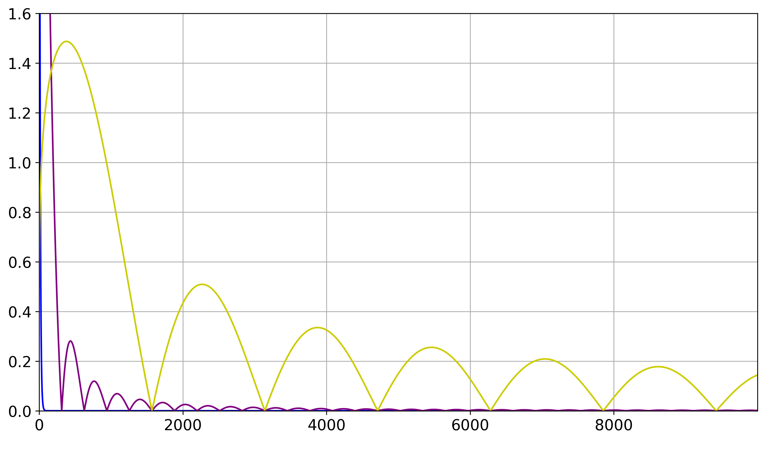
(c) Signals

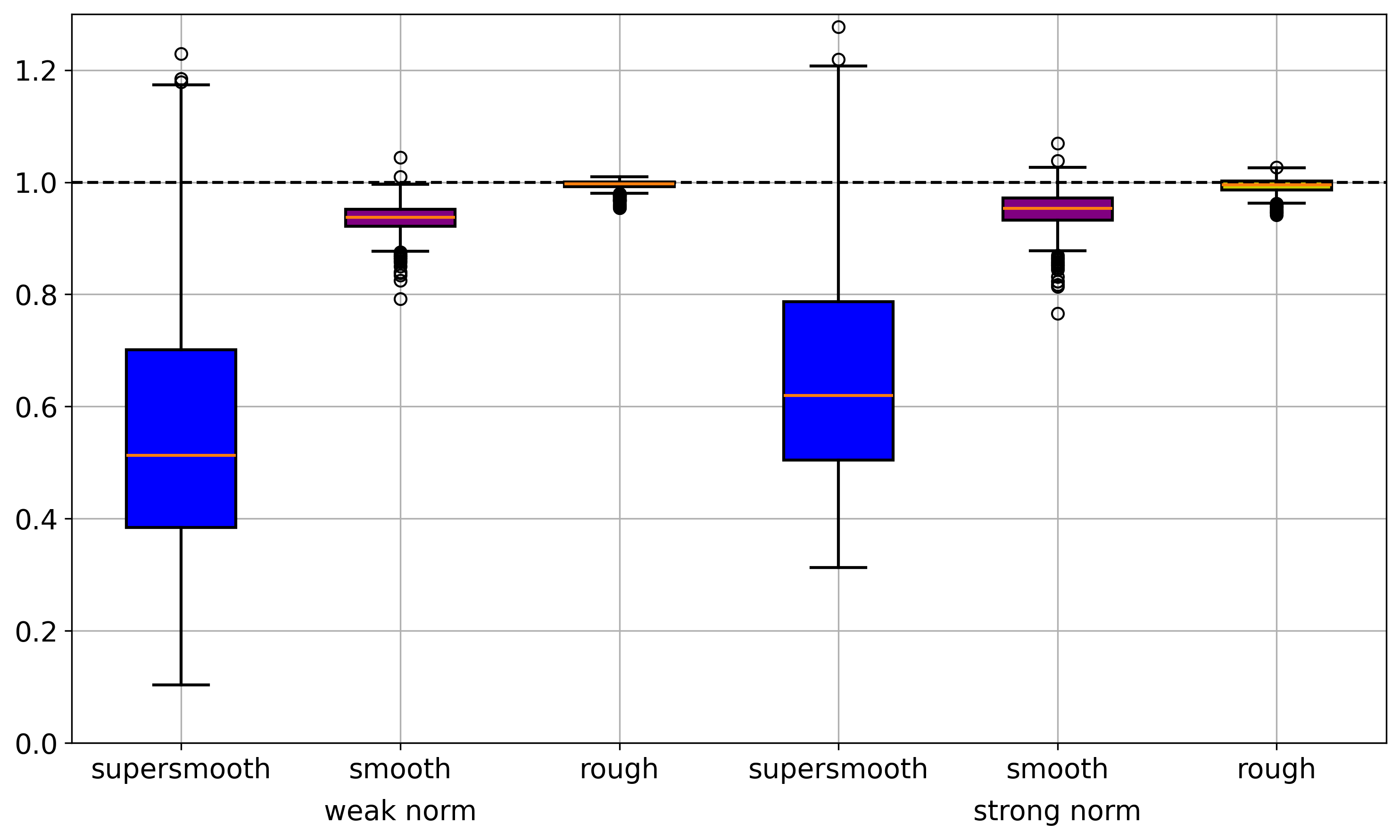
(d) Relative efficiency

Figure 2: Weak (a) and strong risk decomposition (b) for the smooth signal, with bias (blue), variance (red), error (black), balanced oracle (orange), and stopping time (green). (c) SVD representation of a super-smooth (blue), a smooth (purple), and a rough (olive) signal. (d) Relative efficiency: (3.1).

By further defining a diagonal design matrix with $\lambda_{j}=j^{-1/2}$ for $j=1,\dots,p$, multiplying it with a signal from LABEL:code:define_signal and adding noise, we can now define the response variable for the statistical inverse problem (2.5).

⬇

true_noise_level = 0.01

noise = true_noise_level * np.random.normal(0, 1, sample_size)

eigenvalues = 1 / np.sqrt(indices)

from scipy.sparse import dia_matrix

design = dia_matrix(np.diag(eigenvalues))

response = eigenvalues * true_signal + noise

The data from LABEL:code:setup_data and LABEL:code:define_signal is fed into the class associated with the desired iterative estimation procedure, in this case the TruncatedSVD class, and executes a specified number of iterations through the iterate-method.

⬇

alg = es.TruncatedSVD(design, response, true_signal, true_noise_level,

diagonal=True)

alg.iterate(number_of_iterations=3000)

Several base attributes in the TruncatedSVD-class and several theoretical quantities, for example, the strong and weak bias and variance from (2.17), are now available since true_signal and true_noise_level were both specified. The strongly and weakly balanced oracles are computed by applying alg.get_weak_balanced_oracle and alg.get_strong_balanced_oracle, respectively.

⬇

weak_variance = alg.weak_variance

weak_bias2 = alg.weak_bias2

weak_balanced_oracle = alg.get_weak_balanced_oracle(max_iteration=3000)

strong_variance = alg.strong_variance

strong_bias2 = alg.strong_bias2

strong_balanced_oracle = alg.get_strong_balanced_oracle(max_iteration=3000)

Now that we have computed the oracle quantities, they can easily be compared with the data-driven discrepancy principle from (2.13) obtained by applying alg.get_discrepancy_stop. In fact, we already obtain Figure 2(a) and Figure 2(b) by plotting the weak and strong quantities from LABEL:code:manual_quantities_1, respectively. Using alg.get_estimate, we can obtain the algorithm’s estimate at the determined stopping time.

⬇

critical_value = sample_size * true_noise_level**2

discrepancy_time = alg.get_discrepancy_stop(critical_value,

max_iteration=3000)

estimated_signal = alg.get_estimate(discrepancy_time)

In many cases, it is not necessary to manually collect the different parameters from LABEL:code:manual_quantities_1 and LABEL:code:manual_quantities_2. Instead, if we wish to perform a complete Monte-Carlo simulation study and would like to collect all theoretical quantities, we can use the SimulationWrapper. It is most easily used in combination with the SimulationParameters class, which is set up in LABEL:code:setup_data_simulation_parameters.

⬇

parameters_smooth = es.SimulationParameters(design=design,

true_signal=true_signal, true_noise_level=0.01,

monte_carlo_runs=500, cores=10)

We can now create a SimulationWrapper object from the SimulationParameters and run the simulation based on the TruncatedSVD class. The data_set_name parameter of the functions running the simulation, e.g. run_simulation_truncated_svd, is optional and is used to save the simulation results as a .csv file. If the parameter is not specified, the results will not be saved and are returned as a pd.DataFrame.

⬇

simmulation_results = simulation_smooth.run_simulation_truncated_svd(

max_iteration=500, diagonal=True)

Using this methodology, we can replicate the results from Blanchard et al. (2018a) based on the TruncatedSVD-class. The Monte-Carlo experiment is performed using the super smooth, smooth and rough signals in Figure 2(c) and $M=500$ Monte-Carlo iterations. The noise level is set to $\delta=0.01$, and the dimension is chosen as $n=10,000$. The threshold is set as $\kappa=n\delta^{2}=1$. Figure 2(d) illustrates the relative efficiency in RMSE as

$$\text{min}_{m\geq 0}\mathbb{E}[\|\widehat{f}^{(m)}-f^{*}\|^{2}_{A}]^{1/2}/\mathbb{E}[\|\widehat{f}^{(\tau^{\text{DP}})}-f^{*}\|^{2}_{A}]^{1/2},\quad\quad\ \ \text{weak relative efficiency},$$ (3.1)

$$\text{min}_{m\geq 0}\mathbb{E}[\|\widehat{f}^{(m)}-f^{*}\|^{2}]^{1/2}/\mathbb{E}[\|\widehat{f}^{(\tau^{\text{DP}})}-f^{*}\|^{2}]^{1/2},\quad\quad\ \ \ \text{strong relative efficiency}.$$

These quantities are also automatically computed within the SimulationWrapper-class. The balanced oracle iterations (weak) are (34, 316, 1356), and classical oracle iterations in strong norm are (43, 504, 1331). The results match the results from Blanchard et al. (2018a), and we refer to the former paper for a detailed interpretation of the simulation results.

3.2 Landweber

Since the signals and design from LABEL:code:setup_data and LABEL:code:define_signal are contained within the SimulationData class, they do not need to be created manually, see LABEL:code:setup_data_simulation_data.

⬇

design, response, true_signal = es.SimulationData.diagonal_data(

sample_size=2000, type=”smooth”)

This time, we use the data from LABEL:code:setup_data_simulation_data as an input for the Landweber class. The variables true_signal and true_noise_level are optional and required only for the theoretical analysis. The learning_rate can also be specified in the case of the Landweber class.

⬇

alg = es.Landweber(design, response, learning_rate=1,

true_signal=true_signal,

true_noise_level=true_noise_level)

alg.iterate(number_of_iterations = 3000)

Using the iterate-method, we have further executed a desired number of iterations. Several base attributes in the Landweber-class and several theoretical quantities, for instance, from (2.23) are now available since true_signal and true_noise_level were both specified. Based on the bias and variance from LABEL:code:bias_variance_landweber, the balanced oracles are computed through alg.get_weak_balanced_oracle and alg.get_strong_balanced_oracle, see LABEL:code:manual_quantities_landweber.

⬇

weak_variance = alg.weak_variance

weak_bias2 = alg.weak_bias2

strong_variance = alg.strong_variance

strong_bias2 = alg.strong_bias2

⬇

weak_balanced_oracle = alg.get_weak_balanced_oracle(3000)

strong_balanced_oracle = alg.get_strong_balanced_oracle(3000)

critical_value = sample_size * true_noise_level**2

discrepancy_time = alg.get_discrepancy_stop(critical_value,

max_iteration=3000)

estimated_signal = alg.get_estimate(discrepancy_time)

As in the case of the TruncatedSVD-class, we can use the SimulationWrapper-class in combination with the SimulationParameters class, which is set up in LABEL:code:setup_data_simulation_parameters.

⬇

simulation_smooth = es.SimulationWrapper(**parameters_smooth.__dict__)

simmulation_results = simulation_smooth.run_simulation_landweber(

max_iteration=2000)

The data frame returned by the SimulationWrapper already contains all required information to successfully replicate the simulations of Blanchard et al. (2018b), as illustrated in Figure 3 for $500$ Monte-Carlo iterations, where the noise level is $\delta=0.01$, and the dimension is $n=10.000$. We are interested in the early stopping iteration $\tau^{\text{DP}}$ for the threshold $\kappa=n\delta^{2}=1$. The left plot shows the relative number of iterations in weak and strong norm. The weak balanced oracle iterations are (42, 312, 1074), and the strong balanced oracle iterations are (29, 244, 1185) for the supersmooth, smooth, and rough signals, respectively. The right plot shows the relative efficiencies in analogy to the previous section. For a precise analysis and theoretical interpretation of the results, we refer to Section 4.2 in Blanchard et al. (2018b).

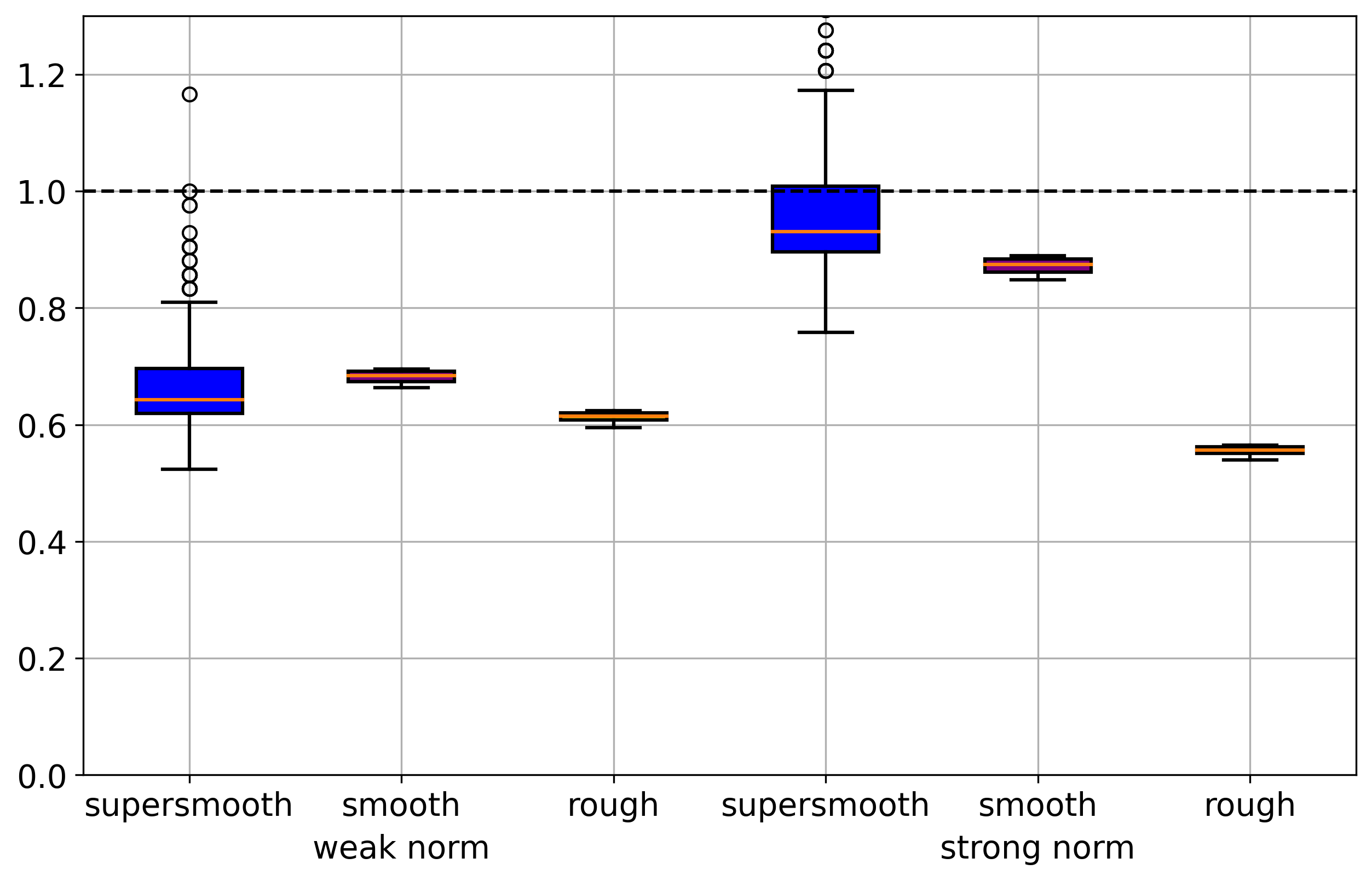
(a) Relative number of iterations

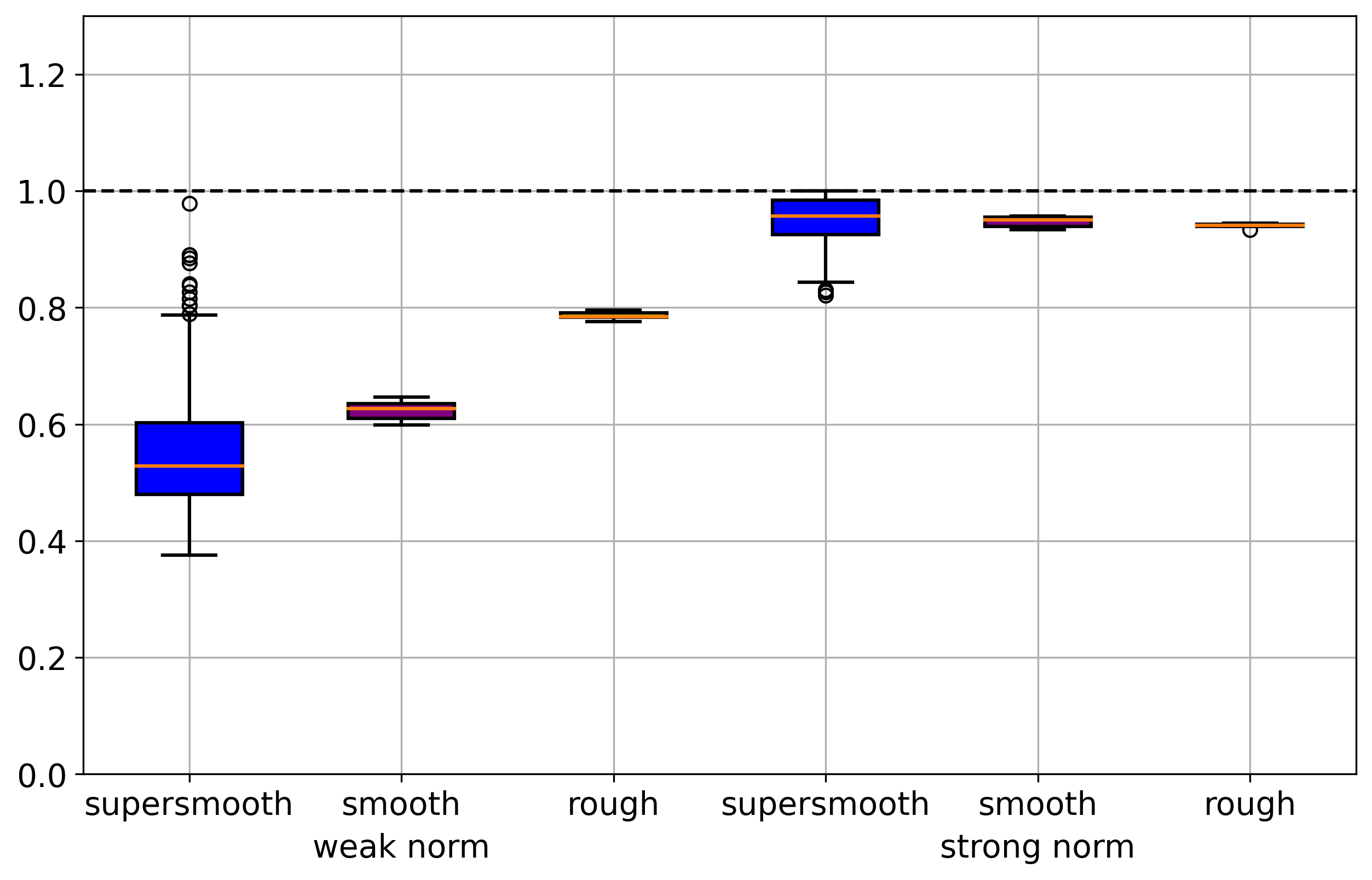
(b) Relative efficiency

Figure 3: (a) Relative number of Landweber iterations for $\tau^{\text{DP}}$ divided by the balanced oracle iteration. (b) Relative efficiency: (3.1).

3.3 Conjugate Gradient Descent

Based on the setup of LABEL:code:init_svd and LABEL:code:init_landweber, we demonstrate the functionality of the ConjugateGradients-class. In LABEL:code:init_cg, a ConjugateGradients instance is initialised analogously to LABEL:code:init_landweber and LABEL:code:init_svd for the Landweber and TruncatedSVD-class, respectively.

⬇

alg = es.ConjugateGradients(design, response, true_signal=true_signal,

true_noise_level=true_noise_level,

computation_threshold = 10 ** (-8))

alg.iterate(number_of_iterations=200)

Note that the additional parameter computation_threshold is required for the emergency stop, as described in Hucker and Reiß (2025). As usual, the iterate-method allows us to execute a specified number of iterations from the conjugate gradient algorithm. In contrast to the Landweber and the TruncatedSVD-class, several of the oracle quantities are empirical and remain dependent on the noise since the associated classical bias-variance decomposition is hard to access. The corresponding empirical quantities can be accessed as described in LABEL:code:empirical_oracle_cg. Note that several quantities allow for an interpolated version, see Remark 2.2.

⬇

strong_empirical_oracle = alg.get_strong_empirical_oracle(max_iteration=200,

interpolation=False)

weak_empirical_oracle = alg.get_weak_empirical_oracle(max_iteration=200,

interpolation=False)

iteration = 100

get_strong_empirical_risk(max_iteration = iteration)

get_weak_empirical_risk(max_iteration = iteration)

The discrepancy stop is obtained in LABEL:code:discrepancy_stop_cg.

⬇

critical_value = sample_size * true_noise_level**2

discrepancy_time = alg.get_discrepancy_stop(critical_value,

max_iteration=100, interpolation=False)

We replicate the simulation study of Hucker and Reiß (2025) for $500$ Monte-Carlo iterations. We can again use the SimulationWrapper-class for the Monte-Carlo simulation, see LABEL:code:wrapper_cg.

⬇

simulation_smooth = es.SimulationWrapper(**parameters_smooth.__dict__)

simmulation_results = simulation_smooth.run_simulation_conjugate_gradients(

max_iteration=2000)

The relative number of iterations and the relative efficiency are illustrated in Figure 4(a) and Figure 4(b), respectively.

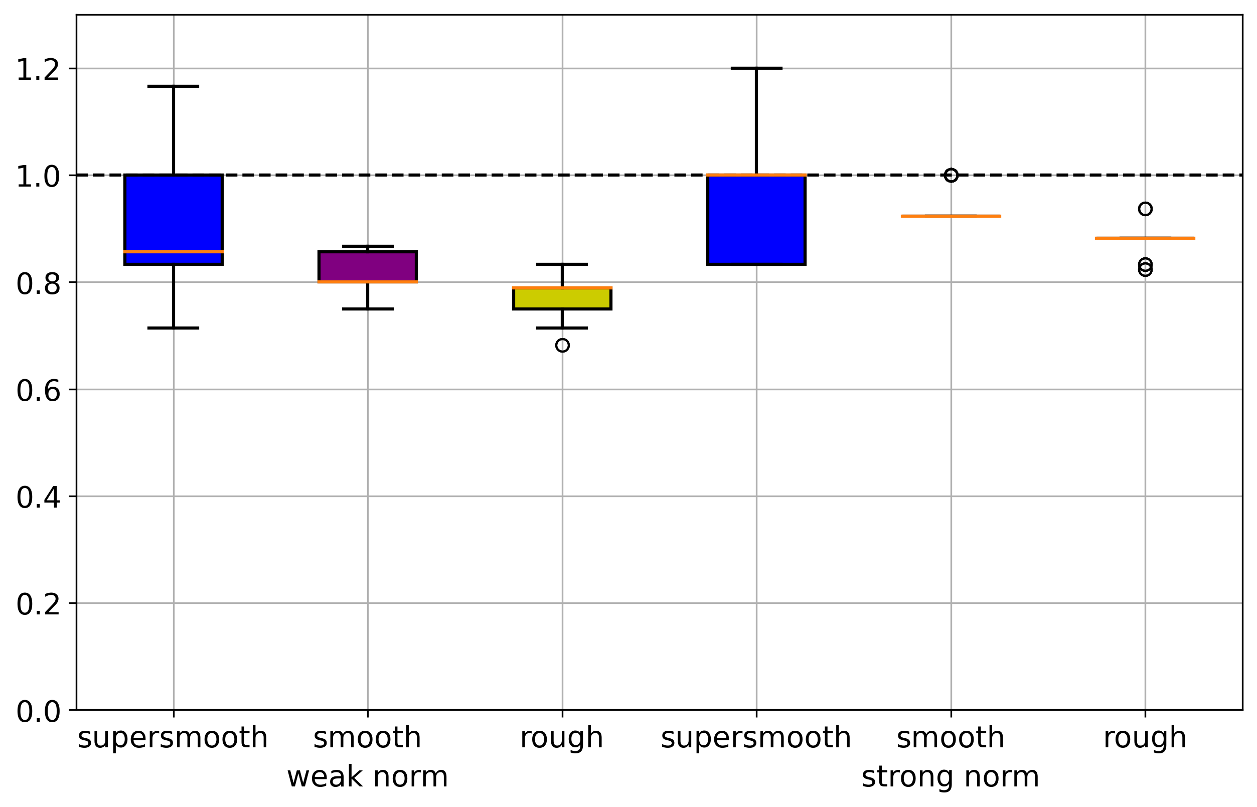
(a) Relative number of iterations

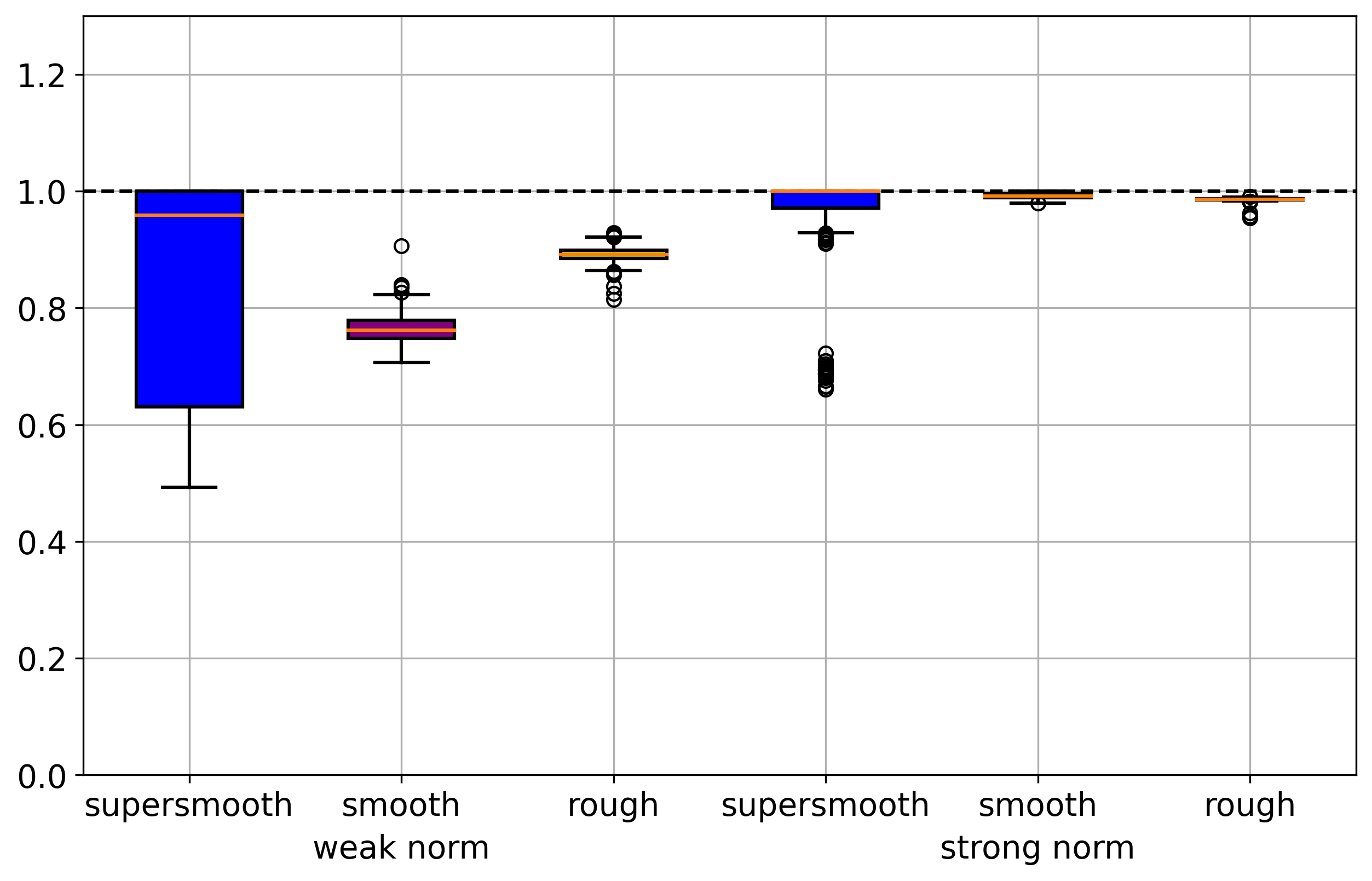
(b) Relative efficiency

Figure 4: (a) Relative number of conjugate gradient iterations for $\tau^{\text{DP}}$ divided by the balanced oracle iteration. (b) Relative efficiency: (3.2).

The quantities in this figure are computed without additional interpolation, which is particularly visible for the supersmooth signal. Note that the weak and strong relative efficiencies are now empirical quantities computed according to:

$$\text{min}_{m\geq 0}\|\widehat{f}^{(m)}-f^{*}\|_{A}/\|\widehat{f}^{(\tau^{\text{DP}})}-f^{*}\|_{A},\quad\quad\text{weak (empirical) relative efficiency},$$ (3.2)

$$\text{min}_{m\geq 0}\|\widehat{f}^{(m)}-f^{*}\|/\|\widehat{f}^{(\tau^{\text{DP}})}-f^{*}\|,\quad\quad\quad\ \text{strong (empirical) relative efficiency}.$$

3.4 $L^{2}$-Boosting

We consider the gamma-sparse and s-spare signals from the simulation in Stankewitz (2024), which are illustrated in Figure 5.

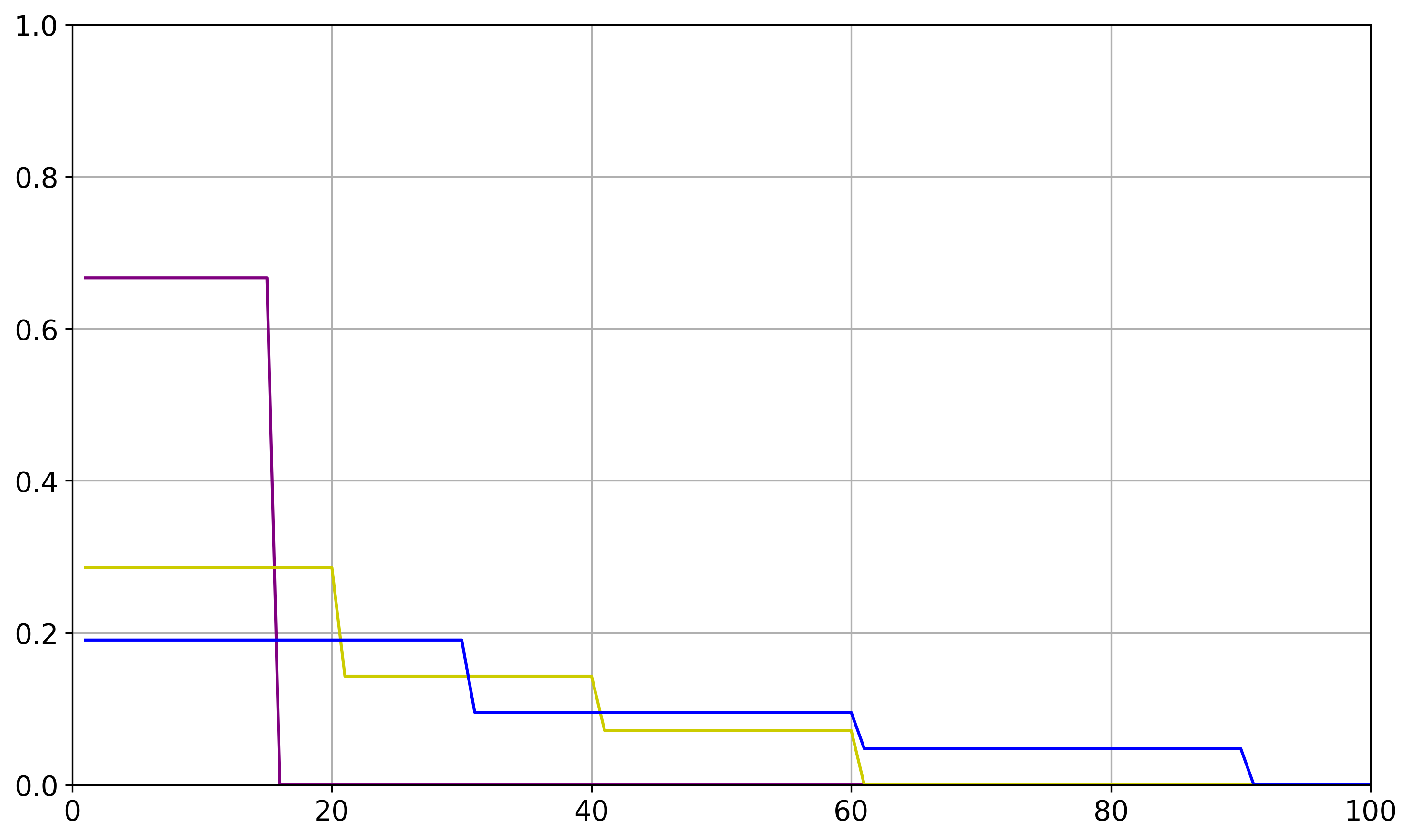
(a) s-sparse signals: $\beta_{15}$ (purple), $\beta_{60}$ (olive), $\beta_{90}$ (blue)

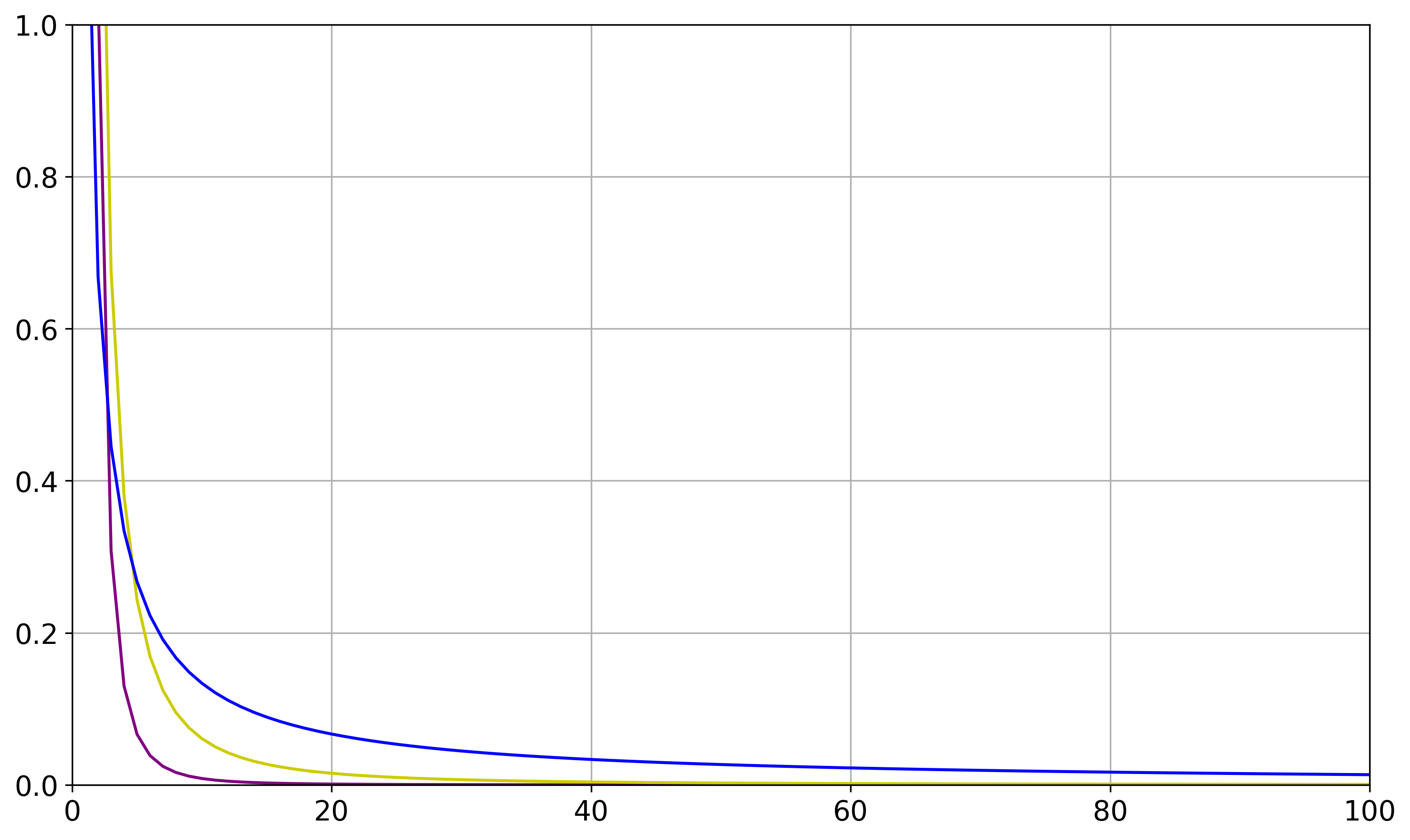
(b) beta-smooth signals: $\beta_{3}$ (purple), $\beta_{2}$ (olive), $\beta_{1}$ (blue)

Figure 5: Signals from the simulation in Stankewitz (2024).

We define one of the signals and simulate data from the high-dimensional linear model (2.29) in LABEL:code:L2-Boost_signals_gamma_sparse.

⬇

sample_size = 1000

parameter_size = 1000

design = np.random.multivariate_normal(np.zeros(parameter_size),

np.identity(parameter_size), sample_size)

beta_3 = 1 / (1 + np.arange(parameter_size)) ** 3

beta_3 = 10 * beta / np.sum(np.abs(beta))

noise = np.random.normal(0, 1, sample_size)

response = design @ beta_3 + noise

In LABEL:code:bosting_usage, we instantiate the L2_boost-class, compute the boosting path up to iteration 500 and access the theoretical quantities from Section 2.2.

⬇

alg = es.L2_boost(design, response, beta_3)

alg.iterate(number_of_iterations = 500)

alg.bias2

alg.stochastic_error

alg.risk

alg.get_balanced_oracle()

For the discrepancy principle in (2.31), the L2_boost-class provides a noise estimation method based on the scaled Lasso algorithm from Sun and Zhang (2012b). The critical_value argument of the method corresponds to $\kappa$ in (2.31). For practical use, this can be set equal to the noise estimate. For the residual ratio stopping method from Kück et al. (2023), the hyperparameter defaults to $K=1.2$ and the confidence level is set to $\alpha=0.95$. The class logs the latest current iteration, here 500, up to which we can query the minimiser of the AIC criterion. The penalty constant defaults to the common choice $K_{\text{AIC}}=2$.

⬇

noise_estimate = alg.get_noise_estimate()

discrepancy_stop = alg.get_discrepancy_stop(critical_value=noise_estimate,

max_iteration=500)

residual_ratio_stop = alg.get_residual_ratio_stop(max_iteration=500, K=1.2,

alpha=0.95)

alg.iteration

alg.get_aic_iteration(K=2, max_iteration = 500)

alg.get_aic_iteration(K=2, max_iteration = discrepancy_stop)

alg.get_aic_iteration(K=2, max_iteration = residual_ratio_stop)

For a newly initialised instance of L2_boost-class, querying one of the sequential stopping times iterates the learning procedure up to that index or the maximal iteration specified. By passing an iteration to the get_aic_iteration-function, we compute the AIC minimiser up to that iteration. For the stopping times, this results in the two-step procedure described in Equation 2.39. The L2_boost class is also featured in the simulation wrapper and Monte-Carlo simulation can be executed as shown in LABEL:code:wrapper_l2_boost.

⬇

parameters_gamma_sparse = es.SimulationParameters(design = design,

true_signal = beta_3, true_noise_level = 1,

monte_carlo_runs = 100, cores=10)

simulation = es.SimulationWrapper(**parameters_gamma_sparse .__dict__)

simmulation_results = simulation.run_simulation_L2_boost(max_iteration=500)

Using this, we can replicate a simulation of the relative efficiencies $\min_{m\geq 0}\|\widehat{f}^{(m)}-f^{*}\|_{n}/\|\widehat{f}^{(\tau)}-f^{*}\|_{n}$ from Stankewitz (2024). Initially, we consider $\tau=\tau^{\text{DP}}$ and $f^{*}=X\beta^{*}$ for a standard Gaussian design matrix $X$ and $\beta^{*}$ one of the signals in Figure 5. Comparing with the results when $\tau=\tau^{(\text{RR})}$ shows that both sequential stopping methods perform reasonably well, with neither outperforming the other over all signals.

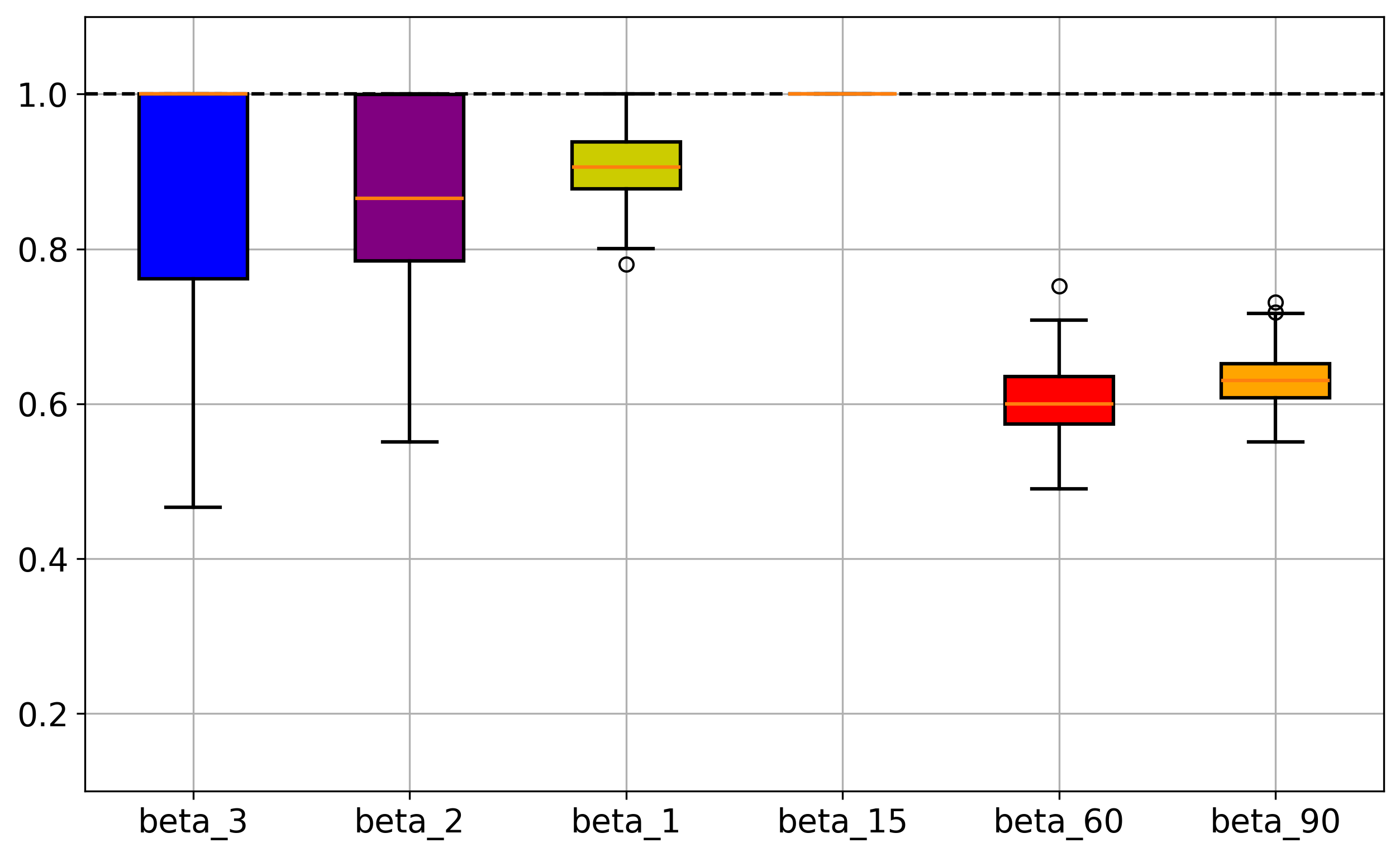
(a) Discrepancy stop.

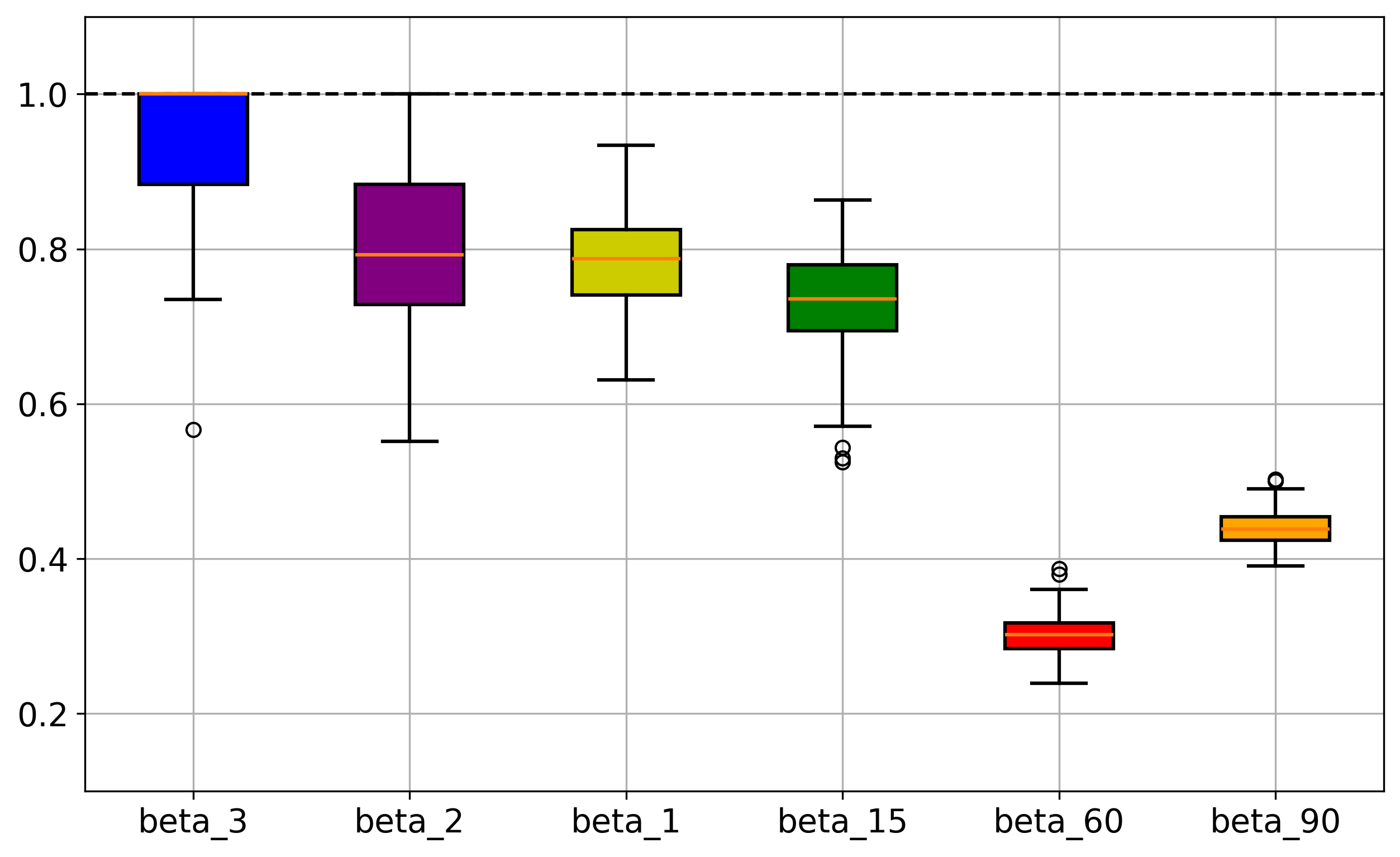
(b) Two-step procedure for the residual ratio stop.

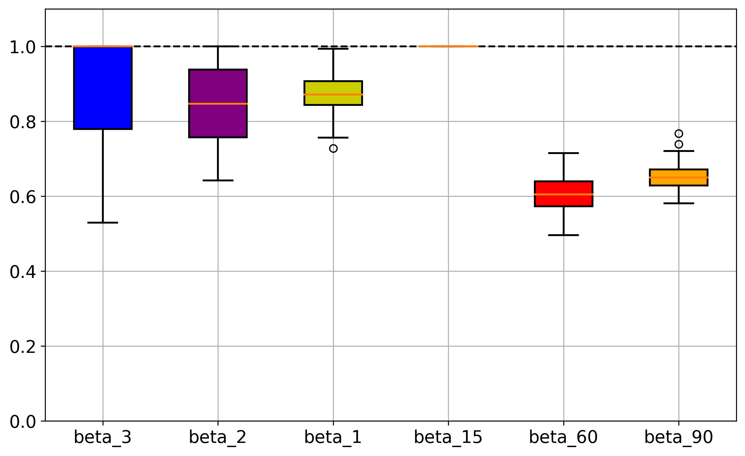
(c) Two-step procedure for the discrepancy stop.

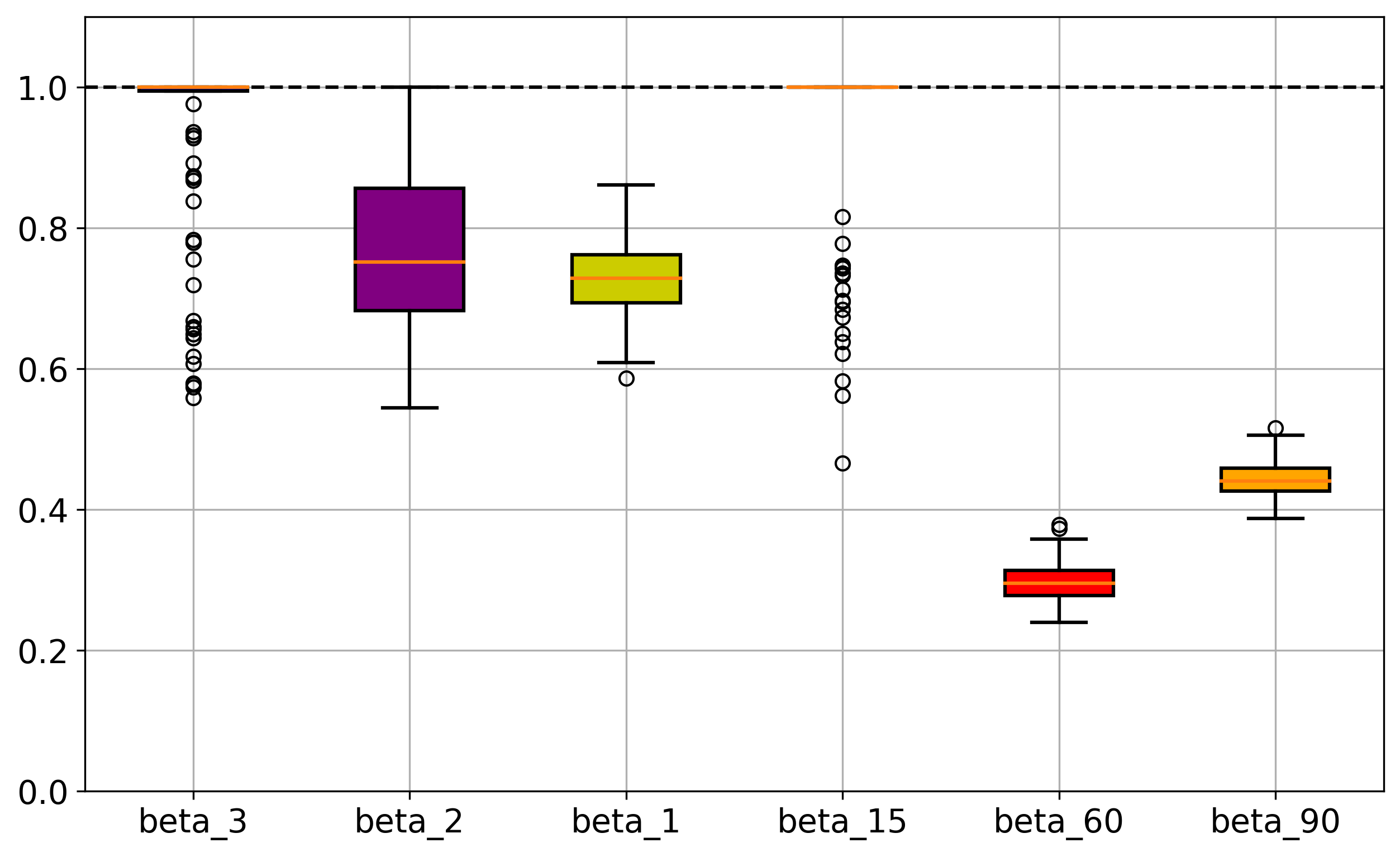
(d) 2-step residual ratio stop

Figure 6: Comparison of the relative efficiencies of the discrepancy stop and the residual ratio stop as well as their associated two-step procedures on the signals from Figure 5.

For the first four signals, stopping tends to be late. Here, both methods profit from combining them with the Akaike criterion in the two-step procedure. For the last two signals, stopping tends to be before the optimal index. Consequently, the two-step procedure cannot provide additional improvement. Again, this underlines the reasoning in Section 2.2 for slightly tuning the algorithm towards larger stopping times. Simulation results in that setting are available in Stankewitz (2024).

3.5 Regression tree

In this section, we replicate the simulation study of Miftachov and Reiß (2025) by using the RegressionTree class. The Monte-Carlo simulation has dimensions $p=30$ with $n=1000$ observations for both the training and the test set. The design is uniformly distributed with $X_{1},\ldots,X_{30}\overset{\mathrm{iid}}{\sim}U(-2.5,2.5)$, $i=1,\ldots,n$ and the response is generated by the additive non-parametric signal

$$f^{*}(x)=g_{1}(x_{1})+g_{2}(x_{2})+g_{3}(x_{3})+g_{4}(x_{4}),\quad x=(x_{1},\ldots,x_{30})^{\top}\in\mathbb{R}^{30}.$$

The functions $g_{j}$, for $j=1,\ldots,4$ are displayed in Figure 7 for different classes of functions.

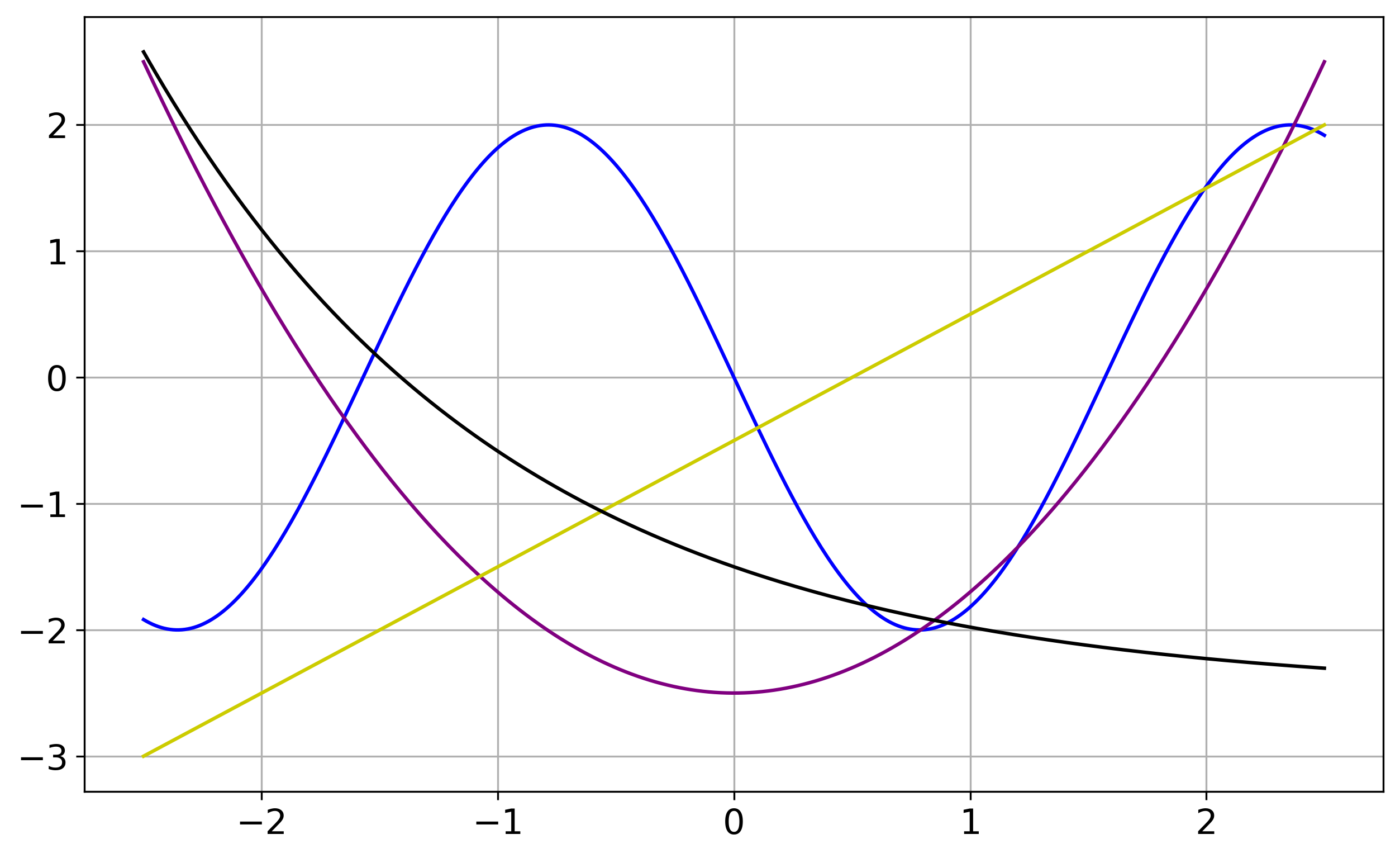
(a) Smooth functions

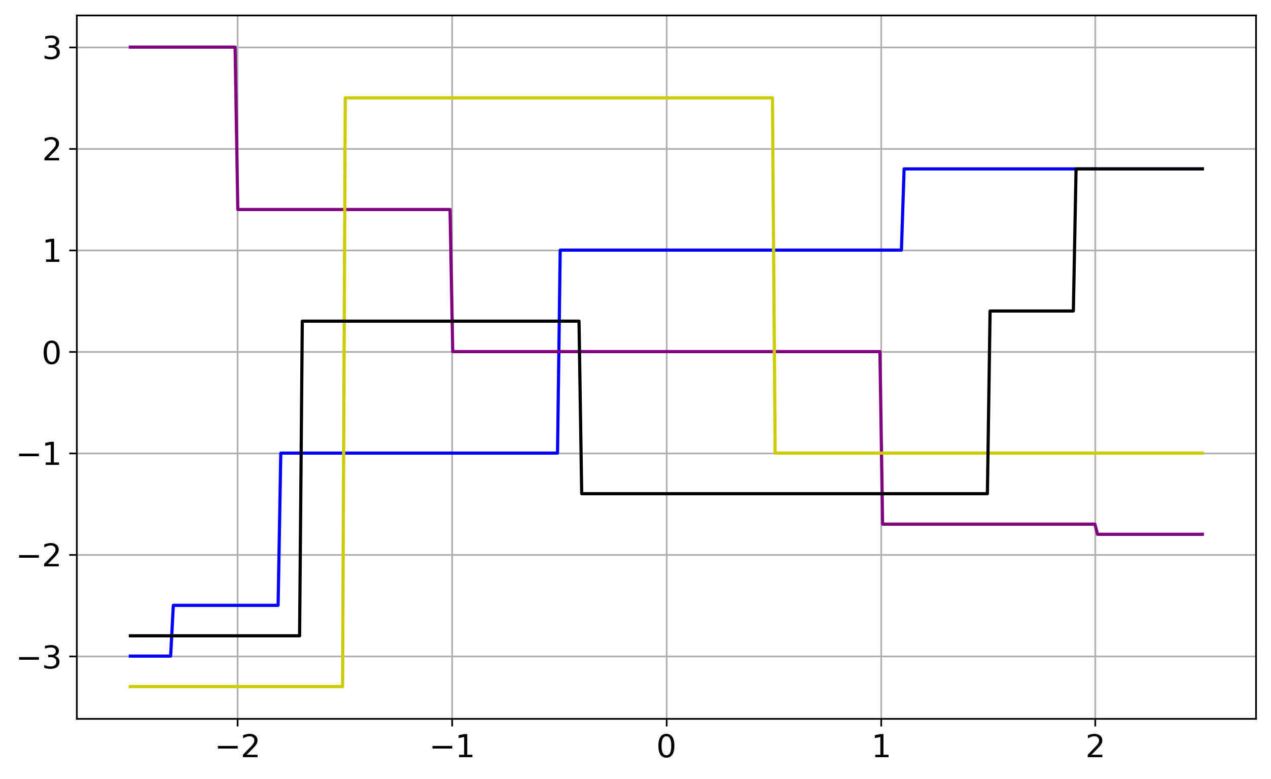
(b) Step functions

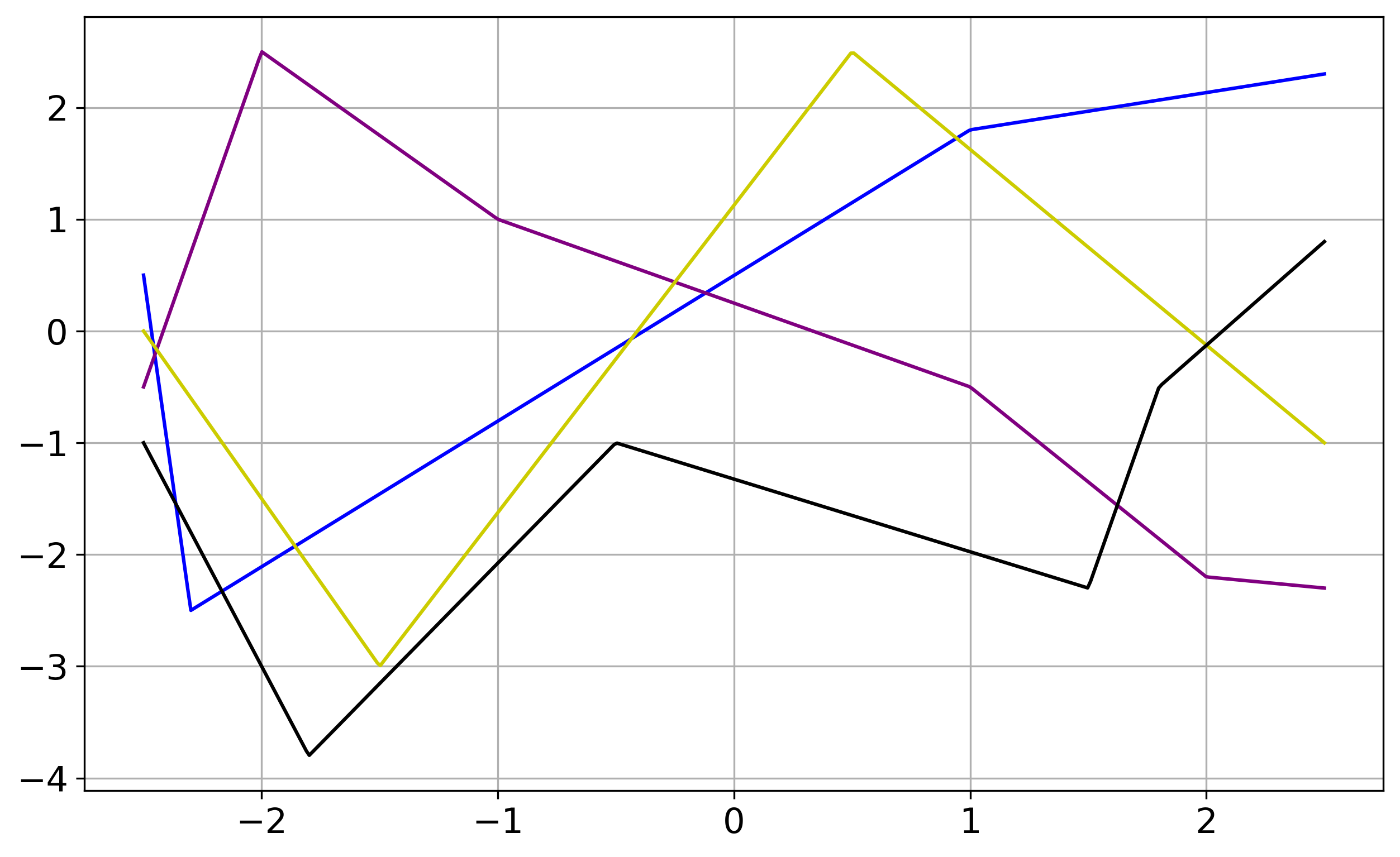
(c) Piecewise linear functions

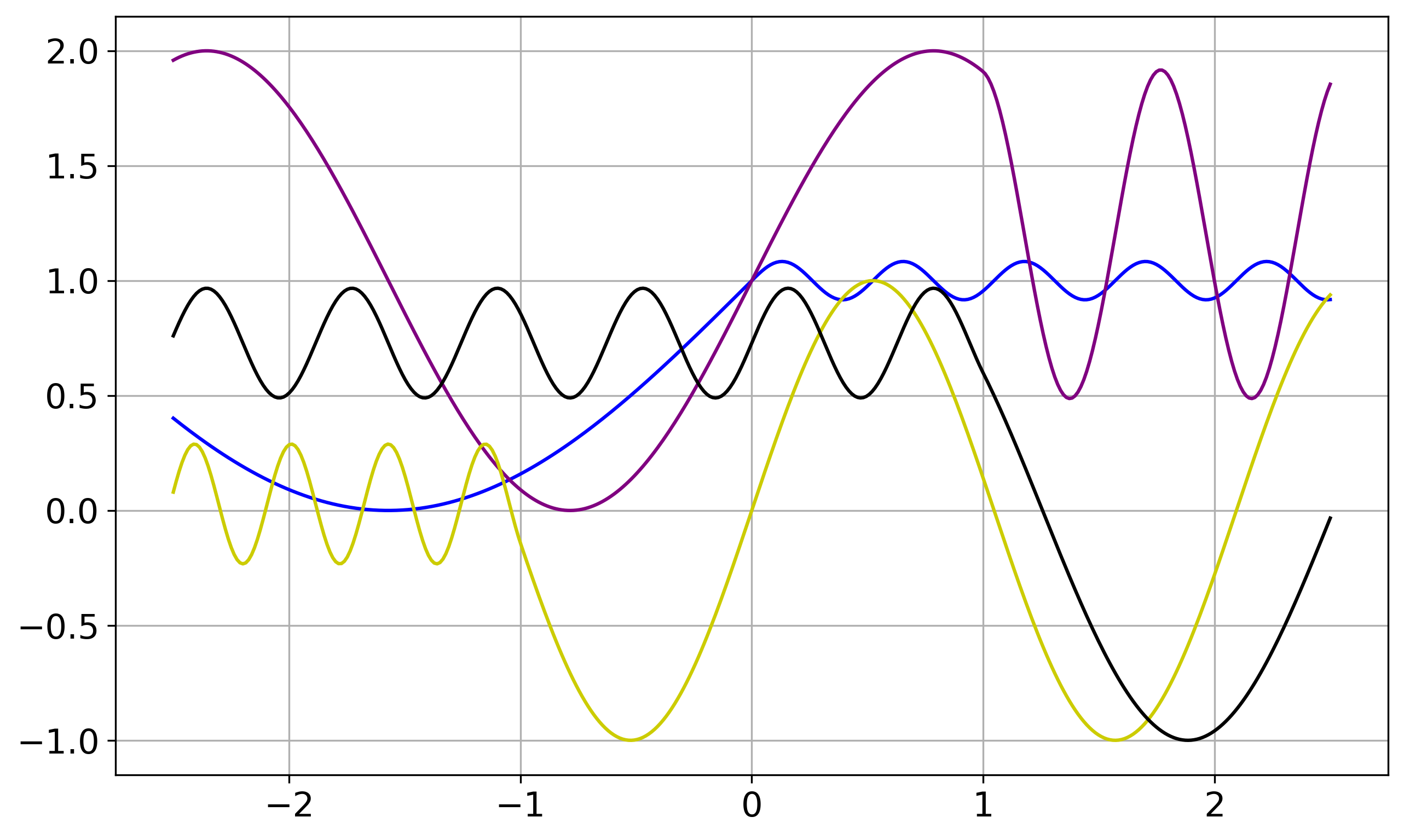
(d) Hills-type functions

Figure 7: Signals $g_{j}$, $j=1,\ldots,4$ in the sparse high-dimensional additive model of the simulation in Miftachov and Reiß (2025).

By using the SimulationData class, these additive models are directly obtained. For example, the smooth additive model is generated by

⬇

sample_size=2000, noise_level=1)

We initialize an instance of RegressionTree in Codeblock LABEL:code:regression_init. Then, the alg.iterate function grows the regression tree, as described in Section 2.3, until reaching the pre-specified max_depth parameter. The non-interpolated stopping iteration, referred to as global early stopping in Miftachov and Reiß (2025), is determined by alg.get_discrepancy_stop.

⬇

alg = es.RegressionTree(design=design, response=response,

min_samples_split=1, true_signal=f, true_noise_vector=noise)

alg.iterate(max_depth=30)

stopping_iteration = alg.get_discrepancy_stop(critical_value=1,

max_depth=30)

The squared bias, the variance and the balanced oracle iteration can be retrieved as shown in LABEL:code:oracle_regression_tree.

⬇

alg.bias2

alg.variance

alg.get_balanced_oracle(max_depth=30)

The regression tree is fitted on a training set and evaluated on an untouched test set, denoted by subscript $n^{\prime}$. The relative efficiency $\min_{t\in[0,n]}\|\widehat{f}_{t}-f\|_{n^{\prime}}/\|\widehat{f}_{\tau}-f\|_{n^{\prime}}$ is calculated for each Monte-Carlo iteration and displayed for each function in Figure 8. The global early stopping is based on the orthogonal projection (2.41), and the interpolated global early stopping uses the projection flow (2.43), see Section 2.3.

We observe in Figure 8 that the interpolation of the regression tree improves prediction performance as the relative efficiency increases. The median relative efficiency is approximately 0.9, which is high for a non-parametric adaptation problem. The reason is that the true underlying function is of sparse additive structure, and as shown in Proposition 1 of Scornet et al. (2015) the CART is able to successfully split only in the relevant coordinate directions. In particular, the sparse components contain relatively strong signals compared to the noise. Thus, the discrepancy principle is able to stop the algorithm very close to the oracle iteration. However, it gets slightly worse for the additive Hills-type functions since the stopping happens too late. This effect is evident from the tables in the simulation of Miftachov and Reiß (2025), as the number of terminal nodes in the early stopped tree is larger than that of the oracle.

For our replication study, we have used the stopping threshold $\kappa=\sigma^{2}$ to obtain the early stopped regression tree. In practice, the noise level $\sigma^{2}$ is usually unknown and must be estimated. A possible approach is the nearest-neighbour estimator proposed by Devroye et al. (2018) and used in Miftachov and Reiß (2025), which is both simple and well-suited for random designs in higher-dimensional settings.

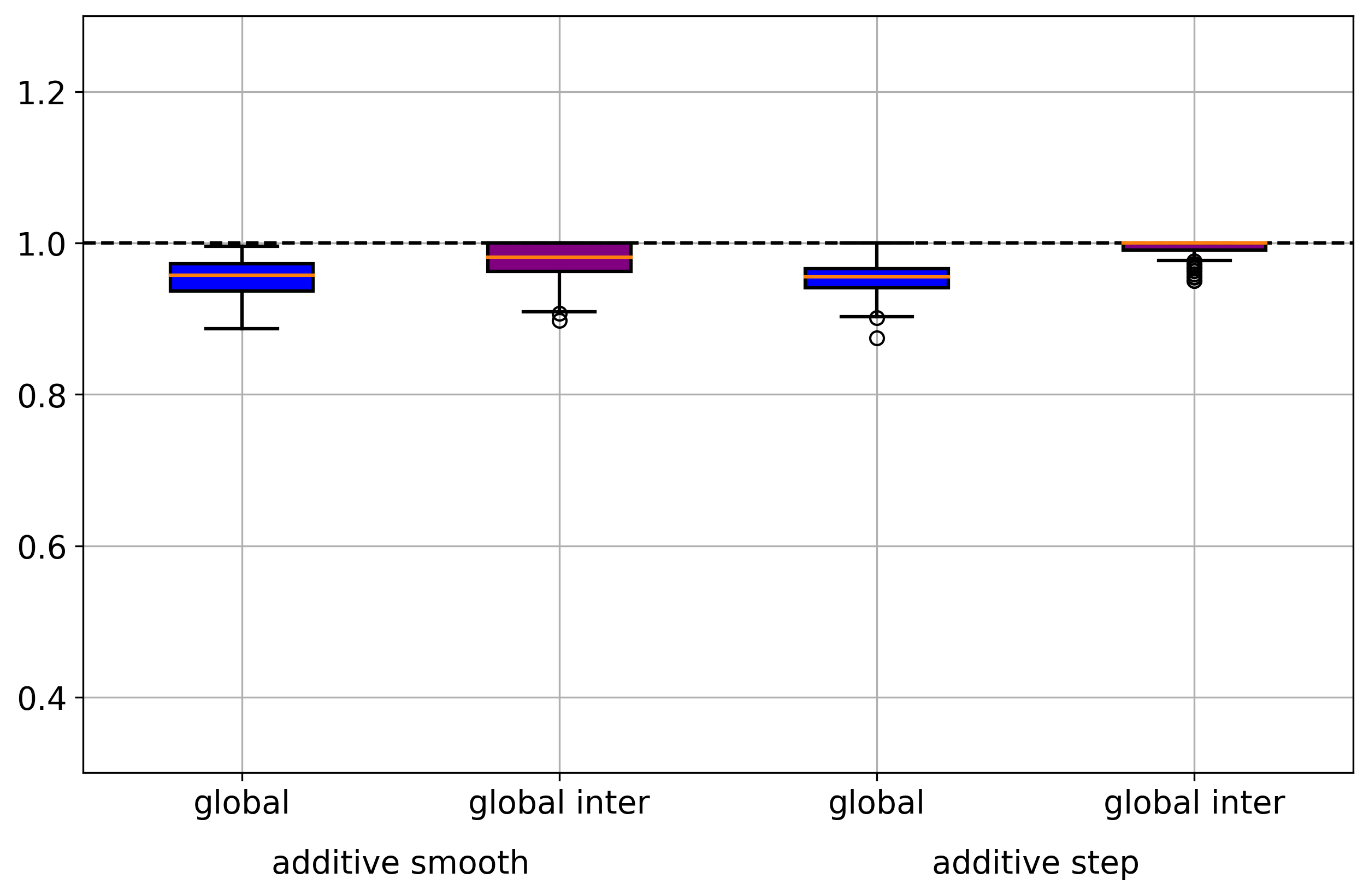
(a) Smooth and step functions

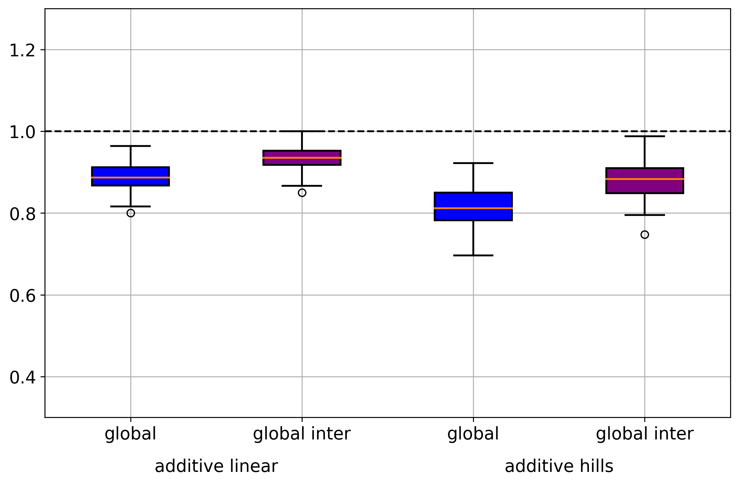
(b) Linear and hills functions

Figure 8: Relative efficiency for the global and interpolated regression tree estimator for different sparse high dimensional additive models, see Miftachov and Reiß (2025). (a) additive smooth and additive step. (b) additive linear and additive hills. Higher values are better.

3.6 Comparison between methods

One of the main contributions of the EarlyStopping-package is that its single coherent framework allows for easy comparisons of different algorithms from the literature. As a simple example, in Figure 9, we compare the different estimates of the smooth signal from Figure 2(c) for the Landweber, TruncatedSVD and ConjugateGradients-classes, respectively. While there is no clear structural difference between the Landweber and ConjugateGradients estimate, the spectral cutoff of TruncatedSVD is markedly visible.

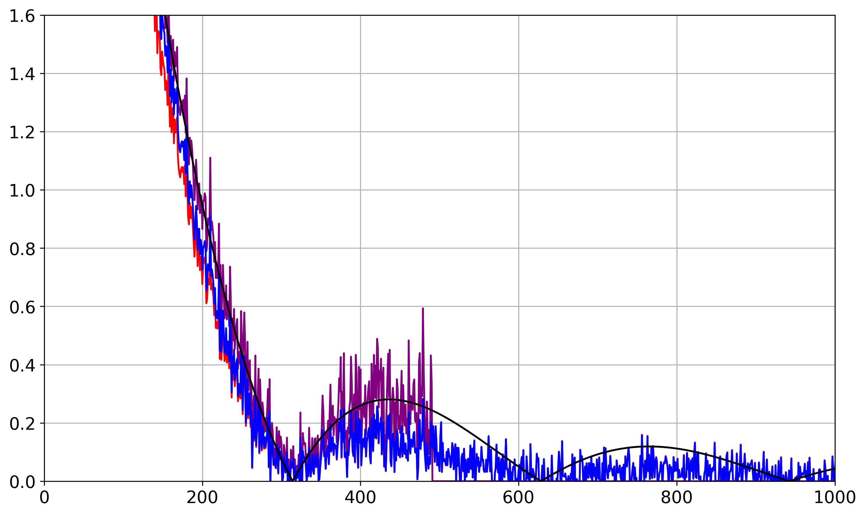
(a) Signal estimate at $\tau$

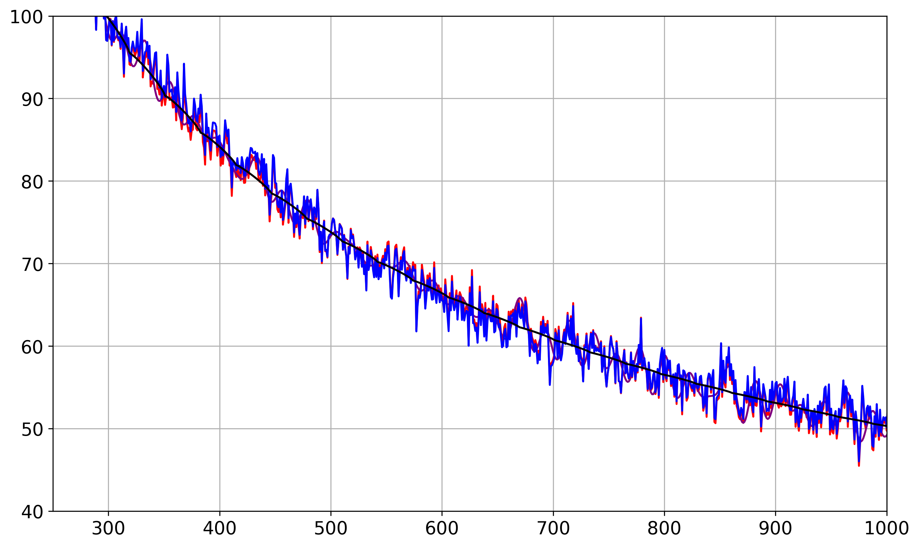
(b) Fourier transform of signal estimate at $\tau$

Figure 9: Different estimated signals for the smooth example in Figure 2. Landweber (blue), tSVD (purple), conjugate gradient (red) and true signal (black).

More interestingly, we can also compare the performance of the same stopping method over the different algorithms. For a somewhat pathological example, let us consider the well-known Phillips’ test problem, which emerges as the discretisation of a Fredholm integral of the first-kind, see Hansen (1994). The true signal $f^{*}$ and design matrix $A$ from the Phillips’ example are visualised in Figure 10.

(a) True signal

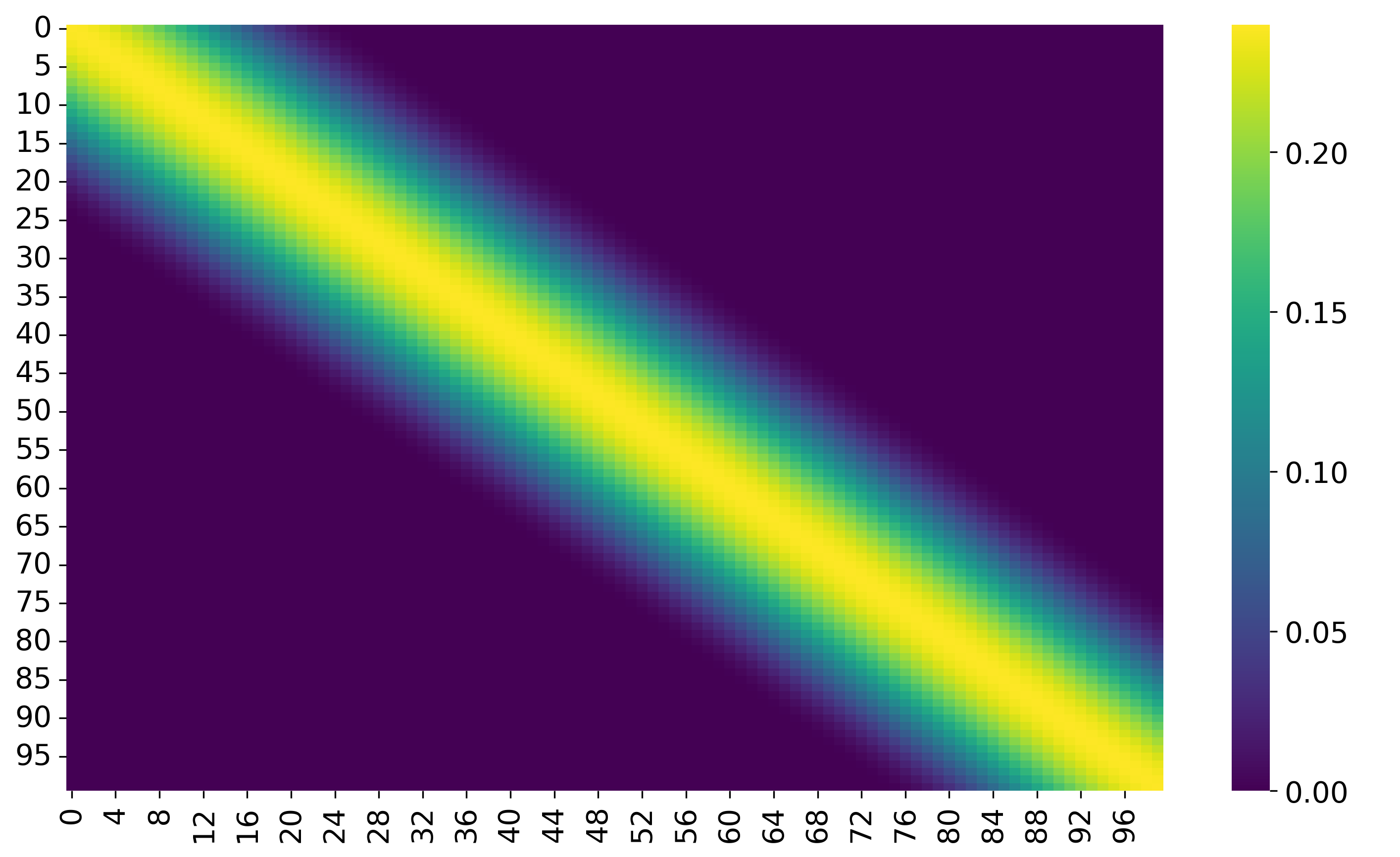
(b) Design

Figure 10: Visualisation of the true signal $f^{*}$ and the design matrix $A$ for the Phillips example.

Figure 11(b) shows a comparison between the strong empirical errors at the discrepancy stop for the Landweber, truncated SVD and conjugate gradient algorithm on Phillips example for $100$ Monte Carlo iterations, $n=100$ and true noise level $\delta=0.1$. Due to its severe ill-posedness, the performance of the estimation procedures is visibly worse than in previous examples, and the deviation of the discrepancy stop from the weak and strong balanced oracle is larger and more susceptible to outliers. Comparatively, the latter effect is particularly severe for the Landweber iteration. Having access to the oracle quantities of the simulation allows us to understand this difference on deeper structural level.

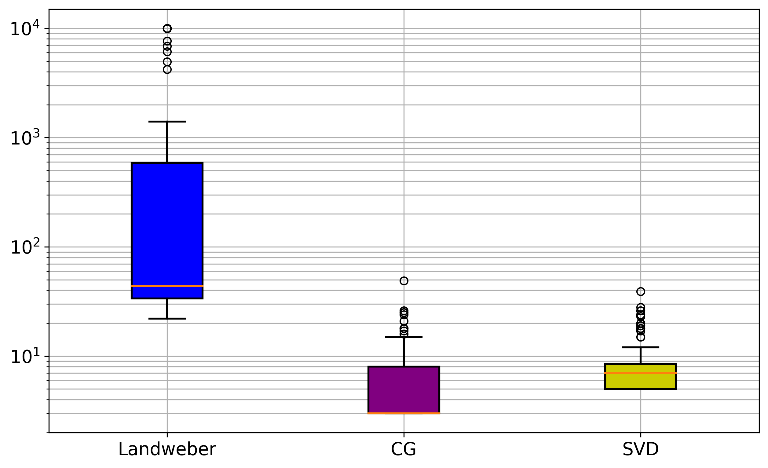
(a) Stopping times

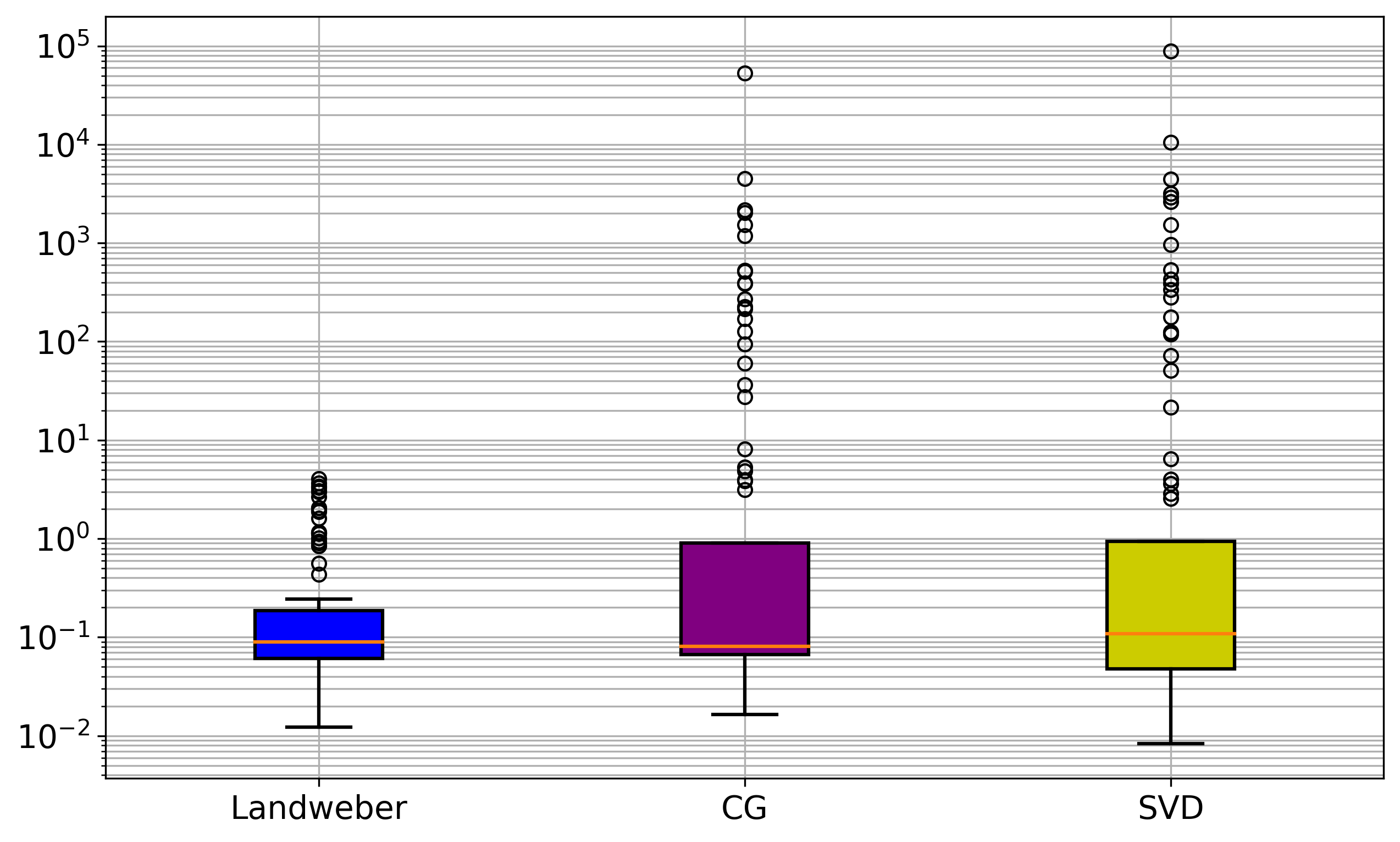
(b) Empirical errors at $\tau^{\text{DP}}$

Figure 11: Comparison of the relative efficiencies and variation of stopping times for the ill-posed Phillips problem from Hansen (1994). Logarithmic scale capped at $10^{4}$.

We consider the truncated SVD procedure first and focus on the weak risk decomposition as the discrepancy stopping time mimics the weak oracle. From (2.19) and the lower bound in Blanchard et al. (2018a), we expect a difference of order $\sqrt{n}\delta^{2}=0.1$ between the optimal risk and the risk at the stopping time, which provides a clear explanation for why the stopping times mostly stay below 50. Both in the weak and the strong risk, this is enough to loose adaptivity. However, this can be salvaged by applying the two-step procedure from (2.21), since we only lose about a factor of five in the computational load from the deviations in the stopping time.

Data	TruncatedSVD	Landweber	ConjugateGradients
Gravity	$1$	0.2	$9\text{e-}4$
Phillips’	$1.8$	0.2	$7.3\text{e-}3$
Smooth	$9\text{e-}4$	$7\text{e-}3$	$2\text{e-}4$
Supersmooth	$8\text{e-}4$	$6\text{e-}3$	$2\text{e-}4$
Rough	$9\text{e-}4$	$6\text{e-}3$	$2\text{e-}4$

Table 1: Average execution time for 100 iterations in seconds.

For the Landweber iteration, this changes structurally. While, as in the case of both versions of the risk for truncated SVD, the strong risk still exhibits a U-shape, this geometry is lost for the weak risk. Consequently, deviations of the size $\sqrt{n}\delta^{2}=0.1$ from the weak optimal risk can result in enormous deviations in the stopping time. The simulation shows deviations up to size $10^{4}$ because this was set as the maximal iteration but even larger times of size $n^{3}=10^{6}$ can occur. This situation, in which the deviations are of the same size $n^{3}$ as the whole learning trajectory constitutes a truly pathological example for early stopping since the two-step procedure becomes qualitatively equivalent to model selection over the full path.

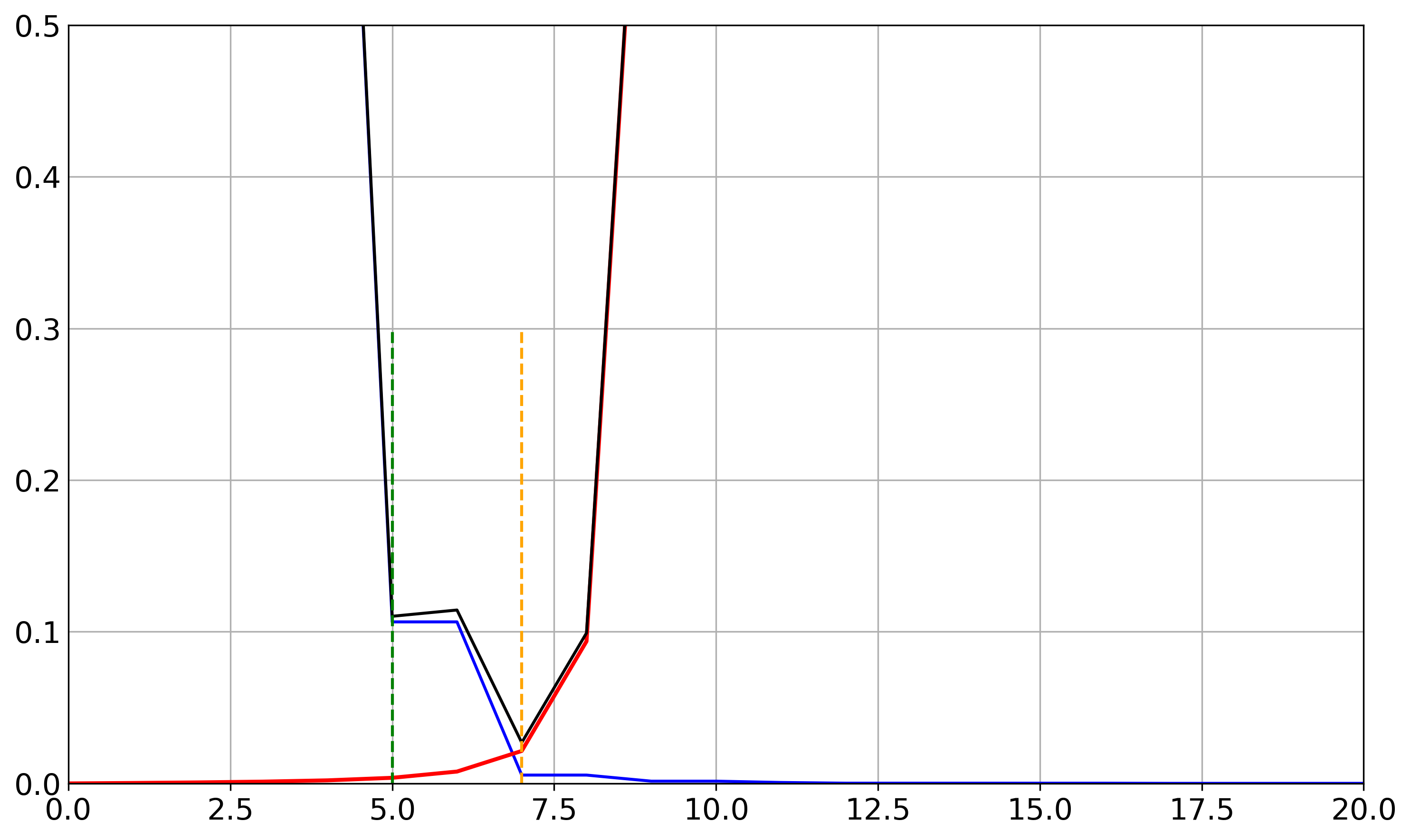
(a) tSVD in strong norm

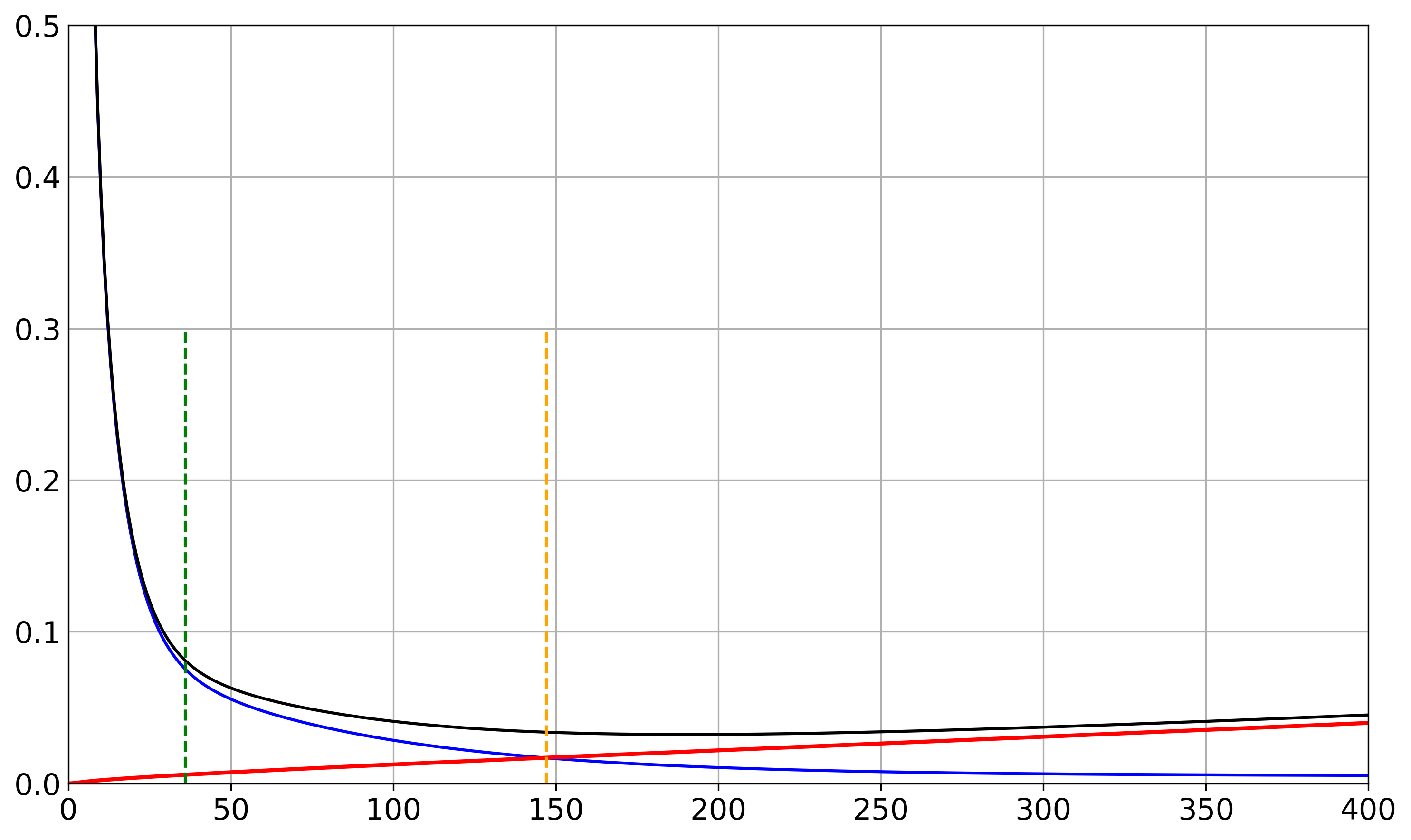
(b) Landweber in strong norm

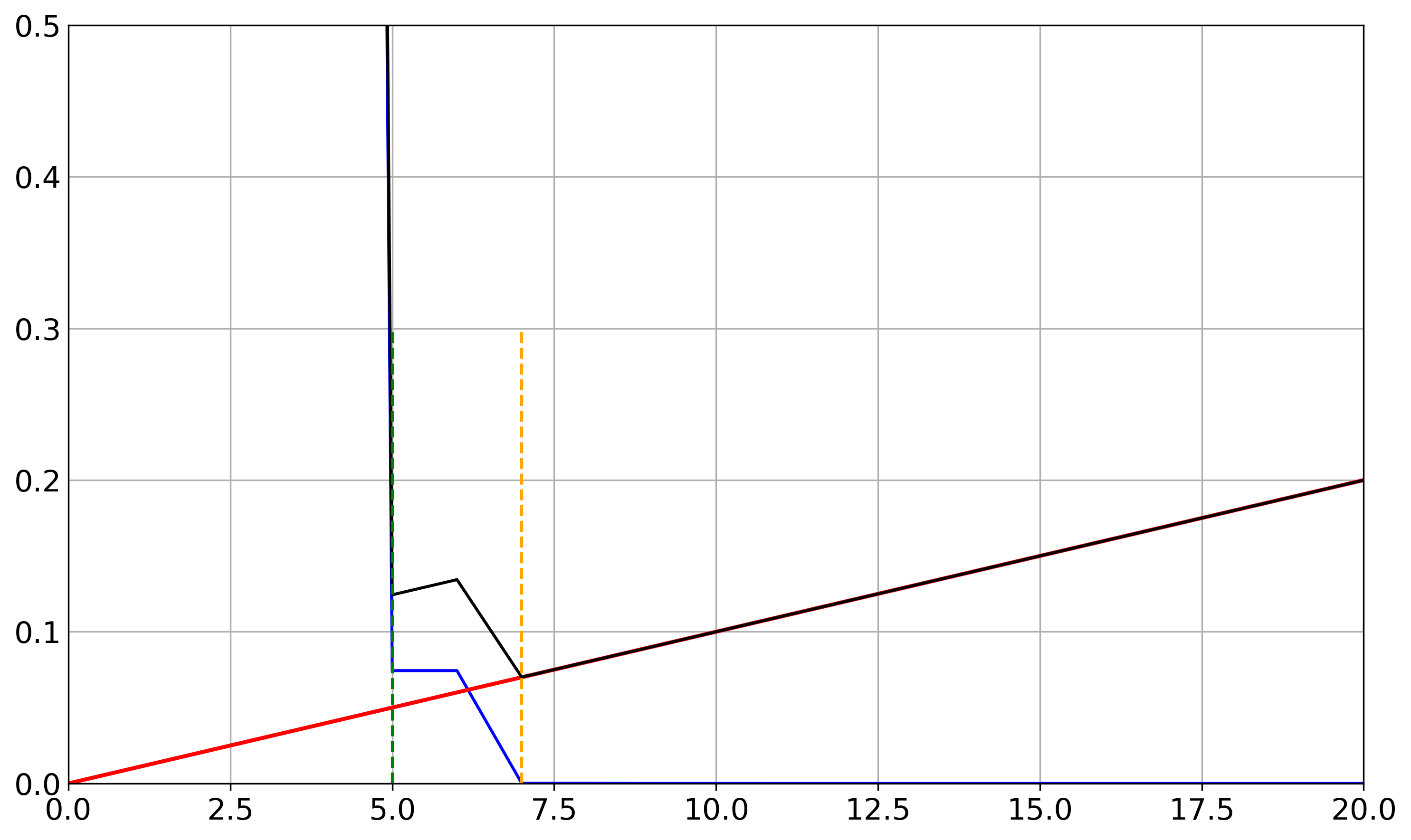
(c) tSVD in weak norm

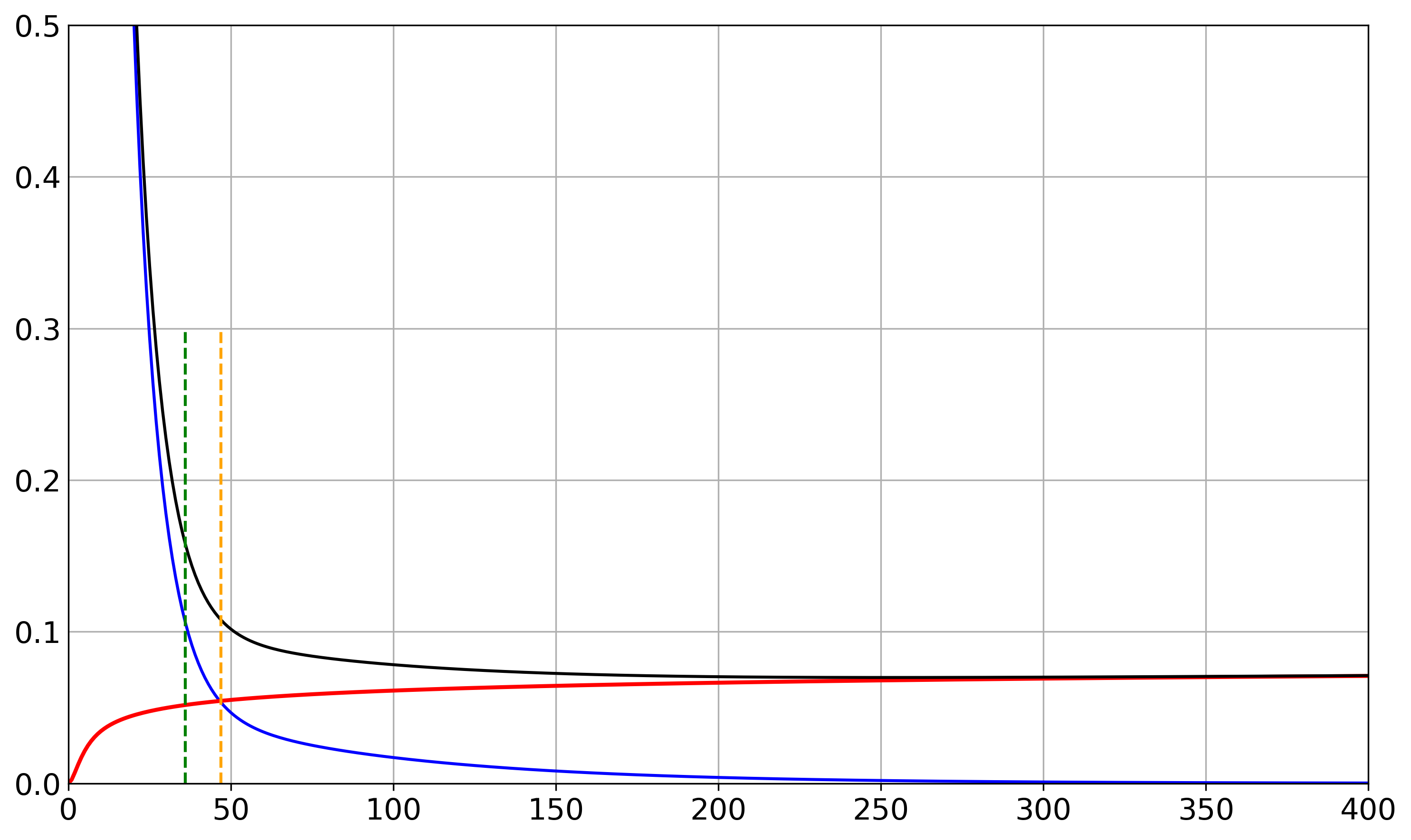
(d) Landweber in weak norm

Figure 12: Comparison of the risk (black), squared bias (blue), variance (red), discrepancy stop (green), balanced oracle (orange) in weak and strong norm for truncated SVD and the Landweber iteration for the Phillips example.

We conclude this section with a brief comparison of the average execution times for 100 iterations of Landweber, ConjugateGradients and TruncatedSVD compared across several different datasets given $n=1000$, see Table 1. Note that these values do not include the additional runtime required for the computation of the theoretical quantities.

References

- Arlot and Celisse [2010] S. Arlot and A. Celisse. A survey of cross-validation procedures for model selection. Statistics Surveys, 4:40–79, 2010.
- Björck [1996] Å. Björck. Numerical methods for least squares problems. Society for Industrial and Applied Mathematics, 1996.
- Blanchard and Mathé [2012] G. Blanchard and P. Mathé. Discrepancy principle for statistical inverse problems with application to conjugate gradient iteration. Inverse Problems, 28(11):115011/1–115011/23, 2012.
- Blanchard et al. [2018a] G. Blanchard, M. Hoffmann, and M. Reiß. Early stopping for statistical inverse problems via truncated svd estimation. Electronic Journal of Statistics, 12(2):3204–3231, 2018a.
- Blanchard et al. [2018b] G. Blanchard, M. Hoffmann, and M. Reiß. Optimal adaptation for early stopping in statistical inverse problems. SIAM/ASA Journal on Uncertainty Quantification, 6(3):1043–1075, 2018b.
- Breiman et al. [1984] L. Breiman, J. Friedman, R. Olshen, and C. J. Stone. Classification and regression trees. Wadsworth, 1984.
- Bühlmann [2006] P. Bühlmann. Boosting for high-dimensional linear models. The Annals of Statistics, 34(2):559–583, 2006.
- Celisse and Wahl [2021] A. Celisse and M. Wahl. Analyzing the Discrepancy Principle for Kernelized Spectral Filter Learning Algorithms. Journal of Machine Learning Research, 22(76):1–59, 2021.
- Chen and Guestrin [2016] T. Chen and C. Guestrin. XGBoost: A scalable tree boosting system. Proceedings of the 22nd ACM SIGKDD International Conference on Knowledge Discovery and Data Mining, 10:785–794, 2016. URL https://xgboost.readthedocs.io/en/stable/.
- Chollet et al. [2015] F. Chollet et al. Keras. https://keras.io, 2015.
- Devroye et al. [2018] L. Devroye, L. Györfi, G. Lugosi, and H. Walk. A nearest neighbor estimate of the residual variance. Electronic Journal of Statistics, 12(1):1752–1778, 2018.
- Engl et al. [1996] H. Engl, M. Hanke, and A. Neubauer. Regularisation of inverse problems. Mathematics and its applications. Kluwer Academic Publishers, 1996.
- Gazzola et al. [2019] S. Gazzola, P. C. Hansen, and J. G. Nagy. Ir tools: a matlab package of iterative regularization methods and large-scale test problems. Numerical Algorithms, 81(3):773–811, 2019. URL https://de.mathworks.com/matlabcentral/fileexchange/95008-irtools.
- Hansen [1994] P. C. Hansen. Regularization tools: A matlab package for analysis and solution of discrete ill-posed problems. Numerical algorithms, 6(1):1–35, 1994. URL https://de.mathworks.com/matlabcentral/fileexchange/52-regtools.
- Harris et al. [2020] C. R. Harris, K. J. Millman, S. J. van der Walt, R. Gommers, P. Virtanen, D. Cournapeau, E. Wieser, J. Taylor, S. Berg, N. J. Smith, R. Kern, M. Picus, S. Hoyer, M. H. van Kerkwijk, M. Brett, A. Haldane, J. F. del Río, M. Wiebe, P. Peterson, P. Gérard-Marchant, K. Sheppard, T. Reddy, W. Weckesser, H. Abbasi, C. Gohlke, and T. E. Oliphant. Array programming with NumPy. Nature, 585(7825):357–362, Sept. 2020. URL http://numpy.org/.
- Hucker and Reiß [2025] L. Hucker and M. Reiß. Early stopping for conjugate gradients in statistical inverse problems. arXiv:2503.05542, 2025.
- Hucker et al. [2025] L. Hucker, M. Reiß, and T. Stark. Comparing regularisation paths of (conjugate) gradient estimators in ridge regression. arXiv:2503.05542, 2025.
- Ing [2020] C. Ing. Model selection for high-dimensional linear regression with dependent observations. The Annals of Statistics, 48(4):1959–1980, 2020.
- Jahn [2022] T. Jahn. Optimal convergence of the discrepancy principle for polynomially and exponentially ill-posed operators for statistical inverse problems. Numerical Functional Analysis and Optimization, 42(2):145–167, 2022.
- Ke et al. [2017] G. Ke, Q. Meng, T. Finley, T. Wang, W. Chen, W. Ma, Q. Ye, and T.-Y. Liu. Lightgbm: A highly efficient gradient boosting decision tree. Advances in neural information processing systems, 30, 2017. URL https://lightgbm.readthedocs.io/en/stable/.
- Klusowski and Tian [2023] J. M. Klusowski and P. M. Tian. Large scale prediction with decision trees. Journal of the American Statistical Association, 119(545):1–27, 2023.
- Kück et al. [2023] J. Kück, Y. Luo, M. Spindler, and Z. Wang. Estimation and inference of treatment effects with l2-boosting in high-dimensional settings. Journal of Econometrics, 234(2):714–731, 2023.
- Lepski et al. [1997] O. V. Lepski, E. Mammen, and V. G. Spokoiny. Optimal spatial adaptation to inhomogeneous smoothness: an approach based on kernel estimates with variable bandwidth selectors. The Annals of Statistics, 25(3):929–947, 1997.
- McKinney et al. [2010] W. McKinney et al. Data structures for statistical computing in python. SciPy, 445(1):51–56, 2010. URL https://pandas.pydata.org/.
- Miftachov and Reiß [2025] R. Miftachov and M. Reiß. Early stopping for regression trees. arXiv:2502.04709, 2025.
- Mika and Szkutnik [2021] G. Mika and Z. Szkutnik. Towards adaptivity via a new discrepancy principle for poisson inverse problems. Electronic journal of statistics, 15:2029–2059, 2021.
- Pasha et al. [2024] M. Pasha, S. Gazzola, C. Sanderford, and U. O. Ugwu. Trips-py: Techniques for regularization of inverse problems in python. Numerical Algorithms, pages 1–38, 2024. URL https://github.com/mpasha3/trips-py.
- Paszke [2019] A. Paszke. Pytorch: An imperative style, high-performance deep learning library. arXiv:1912.01703, 2019. URL https://pytorch.org/.
- Pedregosa et al. [2011] F. Pedregosa, G. Varoquaux, A. Gramfort, V. Michel, B. Thirion, O. Grisel, M. Blondel, P. Prettenhofer, R. Weiss, V. Dubourg, et al. Scikit-learn: machine learning in python. Journal of Machine Learning Research, 12(10):2825–2830, 2011. URL https://scikit-learn.org/1.5/index.html.
- Prechelt [2002] L. Prechelt. Early stopping - but when? In Neural Networks: Tricks of the Trade, pages 55–69. Springer, 2002.
- Raskutti et al. [2011] G. Raskutti, M. Wainwright, and B. Yu. Minimax rates of estimation for high-dimensional linear regression over -balls. IEEE Transactions on Information Theory, 57(10):6976–6994, 2011.
- Scornet et al. [2015] E. Scornet, G. Biau, and J.-P. Vert. Consistency of random forests. The Annals of Statistics, 43(4):1716–1741, 2015.
- Stankewitz [2020] B. Stankewitz. Smoothed residual stopping for statistical inverse problems via truncated svd estimation. Electronic Journal of Statistics, 14(2):3396–3428, 2020.
- Stankewitz [2023] B. Stankewitz. Early stopping for iterative estimation procedures, 2023. PhD-Thesis, Humboldt-Universität zu Berlin.
- Stankewitz [2024] B. Stankewitz. Early stopping for -boosting in high-dimensional linear models. The Annals of Statistics, 52(2):491–518, 2024.
- Stoica and Selen [2004] P. Stoica and Y. Selen. Model-order selection: a review of information criterion rules. IEEE Signal Processing Magazine, 21(4):36–47, 2004.
- Sun and Zhang [2012a] T. Sun and C.-H. Zhang. Scaled sparse linear regression. Biometrika, 99(4):879–898, 2012a.
- Sun and Zhang [2012b] T. Sun and C.-H. Zhang. Scaled sparse linear regression. Biometrika, 99(4):879–898, 2012b.
- Tibshirani [1996] R. Tibshirani. Regression shrinkage and selection via the lasso. Journal of the Royal Statistical Society Series B: Statistical Methodology, 58(1):267–288, 1996.
- Virtanen et al. [2020] P. Virtanen, R. Gommers, T. E. Oliphant, M. Haberland, T. Reddy, D. Cournapeau, E. Burovski, P. Peterson, W. Weckesser, J. Bright, S. J. van der Walt, M. Brett, J. Wilson, K. J. Millman, N. Mayorov, A. R. J. Nelson, E. Jones, R. Kern, E. Larson, C. J. Carey, İ. Polat, Y. Feng, E. W. Moore, J. VanderPlas, D. Laxalde, J. Perktold, R. Cimrman, I. Henriksen, E. A. Quintero, C. R. Harris, A. M. Archibald, A. H. Ribeiro, F. Pedregosa, P. van Mulbregt, and SciPy 1.0 Contributors. SciPy 1.0: Fundamental algorithms for scientific computing in python. Nature Methods, 17:261–272, 2020. URL https://scipy.org/.
- Werner [2018] F. Werner. Adaptivity and oracle inequalities in linear statistical inverse problems: a (numerical) survey. In New trends in parameter identification for mathematical models, pages 291–316. Springer, 2018.