Optimal Nonlinear Online Learning under Sequential Price Competition via $s$-Concavity

Abstract

We consider price competition among multiple sellers over a selling horizon of $T$ periods. In each period, sellers simultaneously offer their prices and subsequently observe their respective demand that is unobservable to competitors. The demand function for each seller depends on all sellers’ prices through a private, unknown, and nonlinear relationship. To address this challenge, we propose a semi-parametric least-squares estimation of the nonlinear mean function, which does not require sellers to communicate demand information. We show that when all sellers employ our policy, their prices converge at a rate of $O(T^{-1/7})$ to the Nash equilibrium prices that sellers would reach if they were fully informed. Each seller incurs a regret of $O(T^{5/7})$ relative to a dynamic benchmark policy. A theoretical contribution of our work is proving the existence of equilibrium under shape-constrained demand functions via the concept of $s$-concavity and establishing regret bounds of our proposed policy. Technically, we also establish new concentration results for the least squares estimator under shape constraints. Our findings offer significant insights into dynamic competition-aware pricing and contribute to the broader study of non-parametric learning in strategic decision-making.

1 Introduction

Pricing plays a central role in competitive markets, where firms continuously adjust prices in response to demand fluctuations and rival strategies. With the rise of algorithmic pricing, companies are increasingly using data-driven methods to optimize pricing decisions. However, many existing pricing algorithms still operate under monopolistic assumptions (Fan et al., 2024; Javanmard & Nazerzadeh, 2019; Golrezaei et al., 2019; Bracale et al., 2025), treating demand as independent of competitors’ actions. This oversimplifies the strategic nature of pricing, where firms dynamically respond to each other in a competitive environment. In reality, pricing is not an isolated decision but an interactive process that requires firms to anticipate and react to competitors’ actions. As highlighted by Li et al. (2024), a major challenge in competition-aware pricing lies in inferring rivals’ pricing behavior from limited observations. Firms cannot easily estimate price sensitivity through controlled experiments since competitors do not coordinate to hold prices constant while one firm tests different price points. Also, designing models that effectively capture competitive effects remains difficult. Although numerous sequential pricing algorithms yield low regret and converge toward Nash equilibrium, they often rely on a linear demand framework (Li et al., 2024). Even approaches that incorporate nonlinear demand typically confine themselves to a specific parametric family with a predetermined nonlinear transformation (Goyal et al., 2023), thereby reducing their applicability.

Motivated by the fact that nonlinear demand models are more realistic and widely studied in various pricing applications (Gallego et al., 2006; Wan et al., 2022; 2023), we extend beyond these limitations by considering a more flexible semi-parametric model where both the parametric and nonparametric components are unknown. We propose a tuning-free algorithm, that achieves sublinear regret with respect to a dynamic benchmark.

In our work, we extend the conventional multi-period pricing framework by incorporating a nonlinear demand model. Here, $N$ sellers simultaneously set prices over $T$ periods, and each seller’s observed demand results from a complex interplay of their own pricing and that of their competitors – a feature that becomes even more pronounced when departing from linearity. Sellers are able to review the pricing history of their rivals, yet they remain unaware of the actual demand those competitors face. We assess performance by comparing the revenue outcomes of our policy against an idealized benchmark where full information is available.

Our study examines pricing policies with two key objectives: (1) assessing whether sellers maximize their revenue over time and (2) analyzing whether seller prices converge to the Nash equilibrium that would arise under full information. To evaluate performance, we measure cumulative regret, defined as the worst-case gap between a seller’s average revenue under our proposed pricing policy (where neither model parameters nor competitor demand is known) and an optimal policy in hindsight (which assumes fixed competitor prices and full knowledge of the demand model).

2 Related Literature and Contributions

2.1 Sequential Price Competition with Demand Learning

Over the past two decades, significant advancements have been made in demand learning within competitive pricing environments. A substantial body of literature exists on price competition under known demand, beginning with the early works of Cournot (1838) and Bertrand (1883), which introduced the classic static models for competition in production output and market price respectively; to different variations such as multinomial logit models (Gallego et al., 2006; Aksoy-Pierson et al., 2013; Gallego & Wang, 2014); fixed-point based methods for mixed-logit demands Morrow & Skerlos (2011); and price competition across multiple decision epochs (Gallego & Hu, 2014; Federgruen & Hu, 2015; Chen & Chen, 2021).

In this paper, we will instead focus on sequential price competition with demand learning. Early foundational work in this area by Kirman (1975) examined a symmetric two-seller competition with linear demand, focusing on unknown demand structures using a model where the expected demands of two firms, given their prices $p_{1}$ and $p_{2}$, are $\lambda_{1}(p_{1},p_{2})=\alpha-\beta p_{1}+\gamma p_{2}$, $\lambda_{2}(p_{1},p_{2})=\alpha-\beta p_{2}+\gamma p_{1}$; and symmetric means that the parameters $\alpha\in\mathbb{R}$ and, $\beta,\gamma\in[0,\infty)$ are shared for the two firms. The case of asymmetric sellers under noisy linear demand was first studied by Cooper et al. (2015) who allowed each seller to learn independently, as if operating like a monopolist. Equilibrium was shown to be attained assuming sellers knew individual price sensitivity, though this is rarely true in practice. In contrast, Li et al. (2024) addressed dynamic pricing with unknown price sensitivities, achieving the optimal regret rate $\sqrt{T}$, under a linear demand model: specifically, firm $i$’s expected demand is $\lambda_{i}(\mathbf{p})=\alpha_{i}-\beta_{i}p_{i}+\sum_{j\in\mathcal{N}\setminus\{i\}}\gamma_{ij}p_{j}$, where $\mathcal{N}=\{1,2,\dots,N\}$, $N$ is the number of firms in the market, $\mathbf{p}=(p_{i})_{i\in\mathcal{N}}$, and $\alpha_{i},\beta_{i},\gamma_{ij}$ are unknown for each $i\in\mathcal{N}$.

However, nonlinear demand models are more realistic and have been used and studied in several models and applications (see e.g. Gallego et al. (2006); Wan et al. (2022; 2023)). For example Gallego et al. (2006) considered the mean demand function $\lambda_{i}(\mathbf{p})\triangleq\frac{a_{i}\left(p_{i}\right)}{\sum_{j}a_{j}\left(p_{j}\right)+\kappa}$ for some known increasing functions $a_{i}$ and real value $\kappa\in(0,1]$. In contrast to prior studies (Li et al., 2024; Kachani et al., 2007; Gallego et al., 2006), we analyze the more general unknown monotone single index expected demand model

$$\lambda_{i}(\mathbf{p})=\psi_{i}\left(-\beta_{i}p_{i}+\sum_{j\in\mathcal{N}\setminus\{i\}}\gamma_{ij}p_{j}\right)=\psi_{i}(-\beta_{i}p_{i}+\bm{\gamma}_{i}^{\top}\mathbf{p}_{-i})=\psi_{i}(\theta_{i}^{\top}\mathbf{p}),$$

for $i\in\mathcal{N}$ where $\mathbf{p}_{-i}\triangleq(p_{j})_{j\in\mathcal{N}\backslash\{i\}}$ and $\theta_{i}$ is a vector of dimension $N$ with $i$-th entry equals to $-\beta_{i}$ and the rest of the entries are the values of $\bm{\gamma}_{i}$ ordered. Here the parameters $(\theta_{i},\psi_{i}(\cdot))_{i\in\mathcal{N}}$ are unknown. This model generalizes the linear demand model by Li et al. (2024); specifically, setting $\psi_{i}(u)=u+\alpha_{i}$ recovers their formulation. Differently from Kachani et al. (2007), the sellers do not share demand information to accomplish the estimation step. We analyze the existence and uniqueness of the Nash Equilibrium (NE) and we prove the convergence of the pricing policy to the NE as well as the rate of convergence of the regret of every single firm relative to a dynamic benchmark policy in our sequential price competition with an arbitrary number of sellers.

2.2 Monotone Single Index Models

Our work is related to the monotone single index model. Specifically, Section˜2.1 describes $N$ monotone single index models $\mathbb{E}(y_{i}|\mathbf{p})=\psi_{i}(\theta_{i}^{\top}\mathbf{p})$, $i\in\mathcal{N}$ with unknown $N$-dimensional parameters $\theta_{i}$ and unknown non-decreasing functions $\psi_{i}(\cdot)$. Unlike generalized linear models (GLMs), which assume that $\psi_{i}$ is known in advance, the single index model, where $\psi_{i}$ is more general a nonlinear function non-necessarily monotone, requires learning $\psi_{i}$ non-parametrically, offering additional flexibility while avoiding the “curse of dimensionality” of fully non-parametric models in high-dimensional settings Zhao (2008). In our setting, we add the requirement that $\psi_{i}$ be non-decreasing. The monotonicity assumption of $\psi_{i}$ here arises naturally: as seen in Section˜2.1, it ensures that demand $\lambda_{i}$ is non-increasing in $p_{i}$ uniformly in $\bm{\gamma}_{i}^{\top}\mathbf{p}_{-i}$. This assumption – namely, that the mean demand for a firm decreases with its own price – is common in economics (see e.g. Birge et al. (2024); Li et al. (2024)). Moreover, the monotonicity assumption of $\psi_{i}$ has a great advantage. Estimators based only on smoothness conditions on the ridge function typically depend on a tuning parameter that has to be chosen by the practitioner. The monotonicity assumption allows non-parametric estimators that are completely data-driven and do not involve any tuning parameters.

The monotone single index model has been studied intensively by Balabdaoui et al. (2019). They proved that the model is identifiable if, for example, $\psi_{i}$ is increasing and $\|\theta_{i}\|_{2}=1$, as long as $\mathbf{p}$ has a density with respect to Lebesgue measure which is strictly positive on its domain (see Balabdaoui et al. (2019, Proposition 5.1)), a condition that we will rely on in this work (see ˜4.1 and discussion in Section˜6.2). They also proposed a (joint) estimator $(\widehat{\theta}_{i,n},\widehat{\psi}_{i,n})$ based on $n$ i.i.d. data points $(y^{(t)},\mathbf{p}^{(t)})$, for which $\widehat{\psi}_{i}(\widehat{\theta}_{i}^{\top}\cdot)$ has rate of order $n^{-1/3}$ in the $L^{2}$ norm. Additionally, they analyze the well-known linear estimator $\widetilde{\theta}_{i,n}=\widehat{\theta}_{i,n}/\|\widehat{\theta}_{i,n}\|_{2}$, where

$$\widehat{\theta}_{i,n}=\ \operatorname{argmin}_{\theta\in\mathbb{R}^{N}}\sum_{t=1}^{n}(y_{i}^{(t)}-\theta^{\top}(\mathbf{p}^{(t)}-\bar{\mathbf{p}}))^{2},\quad\bar{\mathbf{p}}=\frac{1}{n}\sum_{i=1}^{n}\mathbf{p}^{(t)}.$$ (1)

The linear estimator $\widetilde{\theta}_{i}$, which dates back to Brillinger (2012), coincides with what one would use under a purely linear model and remains consistent if $\mathbf{p}^{(t)}$ is drawn from an elliptical distribution.

In this work, we utilize an exploration-exploitation algorithm, where the exploration phase is used to collect data to obtain consistent estimators for $(\theta_{i},\psi_{i})$. Since the data in the exploration phase has a different distribution from the data in the exploitation phase, it typically is not sufficient to have a convergence in $L^{2}$ of $x\mapsto\widehat{\psi}_{i}(\widehat{\theta}_{i}^{\top}x)$ to derive an upper bound on the total regret, while a supremum norm converge is sufficient for this scope. For this reason, we propose to split the exploration phase into two sub-phases for which we separately learn $\theta_{i}$ and $\psi_{i}$, and derive a supremum norm convergence. Concretely, in the first part, we estimate $\theta_{i}$ using the linear estimator in Equation˜1, for which we prove a concentration inequality (see Proposition 6.3), differently from Balabdaoui et al. (2019) that primarily studies convergence in probability and in distribution. In the second part of the exploration phase, we estimate $\psi_{i}$. While a natural choice would be the isotonic estimator (which enforces monotonicity), we impose the additional constraint that $\psi_{i}$ must be $s_{i}$-concave for some $s_{i}>-1$. This extra condition is sufficient for the existence of a Nash Equilibrium in our setting, as discussed below.

2.3 Connection with the Existence of NE, Virtual Valuation Function, and $s$-Concavity

In Lemma˜4.5 we establish the existence of an NE for model in Section˜2.1 under the condition that

$$\varphi_{i}(u)=u+\frac{\psi_{i}(u)}{\psi_{i}^{\prime}(u)},$$ (2)

(aka virtual valuation function) is increasing with derivative bounded away from zero, that is that $\varphi_{i}^{\prime}\geq c_{i}$ for some $c_{i}>0$. The same assumption found in several works with $N=1$, for example, Assumption 2.1 in Fan et al. (2024), Assumption 1 in Chen & Farias (2018), Equation 1 in Cole & Roughgarden (2014) and Golrezaei et al. (2019); Javanmard (2017); Javanmard & Nazerzadeh (2019) which assume $\psi_{i}$ and $1-\psi_{i}$ to be log-concave (which implies specifically $c_{i}\geq 1$), where $\psi_{i}$ here is bounded in $(0,1)$, i.e. it represents a survival function.

While log-concavity is a natural shape restriction, recent work in non-parametric shape-constrained inference has explored natural generalizations to classes of functions that exhibit concavity under transformation by a fixed function. Of particular interest is the notion of $s$-concavity, where the transforming function is driven by the real parameter $s$ and yields log-concavity as $s$ goes to 0 (see Section˜2.4 for more details). Our main observation to establish the existence of a NE in terms of shape constraints on $\psi_{i}$ is that $\varphi_{i}^{\prime}\geq c_{i}$ for some $c_{i}>0$ is equivalent to requiring that $\psi_{i}$ is $(c_{i}-1)$-concave (Lemma˜4.5 and Proposition˜4.3). This observation allows us to leverage the shape-constrained statistical inference for estimating $\psi_{i}$, and then a tuning-parameter-free algorithm. Specifically, we use non-parametric least squares estimation (NPLSE) to estimate $\psi_{i}$ under $s$-concavity. As must be clear from the above discussion but worth restating: this shape-constrained assumption is not an artificial imposition by us; rather, it is implicit in the work of previous researchers. A key advantage of our shape-constrained approach compared to common non-parametric approaches lies in that our estimate can be computed without needing to specify any tuning parameter and is entirely data-driven.

2.4 $s$-Concavity

A technical contribution of this work is the study of the uniform rate of convergence of the least-squares estimator of an $s$-concave regression function. This class of functions includes both concave functions ($s=1$) and log-concave functions ($s=0$). As defined in Han & Wellner (2016), a function $\psi:\mathbb{R}^{d}\rightarrow(0,\infty)$ is said to be $s$-concave for some $s\in\mathbb{R}$ and we write $\psi\in\mathcal{F}_{d,s}$ if

$$\psi\left((1-\theta)u_{0}+\theta u_{1}\right)\geq M_{s}\left(\psi\left(u_{0}\right),\psi\left(u_{1}\right);\theta\right),$$

for all $u_{0},u_{1}\in\mathbb{R}^{d}$ and $\theta\in(0,1)$, where

$$M_{s}(y_{0},y_{1};\theta)\triangleq\begin{cases}((1-\theta)y_{0}^{s}+\theta y_{1}^{s})^{1/s},&s\neq 0,y_{0},y_{1}>0\\ 0,&s<0,y_{0}=y_{1}=0\\ y_{0}^{1-\theta}y_{1}^{\theta},&s=0.\end{cases}$$

This notion generalizes log-concavity which holds for $s=0$, in the sense that $\lim_{s\rightarrow 0}M_{s}(y_{0},y_{1};\theta)=M_{0}(y_{0},y_{1};\theta)$. The class of log-concave densities has been extensively studied: see Bobkov & Madiman (2011); Dümbgen & Rufibach (2009); Cule & Samworth (2010); Borzadaran & Borzadaran (2011); Bagnoli & Bergstrom (2006); Doss & Wellner (2016); Brascamp & Lieb (1976); while Han & Wellner (2016); Doss & Wellner (2016); Chandrasekaran et al. (2009); Koenker & Mizera (2010) deal with general $s$-concavity. It’s easy to see that such functions $\psi$ have the form $\psi=(\phi_{+})^{1/s}$ for some concave function $\phi$ if $s>0$, where $x_{+}=\max\{0,x\}$, $\psi=e^{\phi}$ for some concave function $\phi$ if $s=0$, and $\psi=(\phi_{+})^{1/s}$ for some convex function $\phi$ if $s<0$. These classes are nested since $\mathcal{F}_{d,s}\subset\mathcal{F}_{d,0}\subset\mathcal{F}_{d,r}$, if $-\infty<r<0<s<\infty$. In this paper, we consider the unidimensional case, where $\psi$ represents a mean demand function on a set of prices $\mathcal{P}$ that is positive and strictly increasing, and then $\psi:\mathcal{P}\rightarrow(0,\infty)$ has the form $\psi=h_{s}\circ\phi$ where $\phi:\mathcal{P}\rightarrow\mathbb{R}$ is concave and

$$h_{s}(x)=d_{s}^{-1}(x)=\begin{cases}e^{x},&s=0,x\in\mathbb{R},\\ (-x)^{1/s},&s<0,x<0,\\ x^{1/s},&s>0,x>0,\end{cases}\qquad d_{s}(y)=\begin{cases}\log(y),&s=0,y>0,\\ -y^{s},&s<0,y>0,\\ y^{s},&s>0,y>0.\end{cases}$$ (3)

More precisely, we study the more general class $\mathcal{F}_{h}$ that contains functions of the form $\psi=h\circ\phi$, where $h:\mathbb{R}\rightarrow(0,\infty)$ is a known increasing twice differentiable function and $\phi$ is an unknown concave function. Differently from previous results, we focus on regression problems with mean function in $\mathcal{F}_{h}$. More precisely, in Appendix˜F, we consider i.i.d. observations $(U_{i},Y_{i})\sim(U,Y)$ for $i=1,2,\dots,n$ where $Y_{1},\dots,Y_{n}$ are noisy versions of the mean function $\psi_{0}(u)=\mathbb{E}\left(Y|U=u\right)=h(\phi_{0}(u))$ and $U_{1}\leq U_{2}\leq\dots\leq U_{n}$ for some unknown concave $\phi_{0}:\mathcal{U}\rightarrow\mathbb{R}$ and a known increasing twice differentiable transformation $h:\mathbb{R}\rightarrow(0,\infty)$ (i.e. $\psi_{0}\in\mathcal{F}_{h}$), where $\mathcal{U}$ is an interval containing $\mathcal{T}=\left\{U_{1},U_{2},\ldots,U_{n}\right\}$. We study the uniform convergence rate of $\widehat{\psi}_{n}=h\circ\widehat{\phi}_{n}$, where $\widehat{\phi}_{n}$ is the LSE

$$\widehat{\phi}_{n}\in\operatorname{argmin}_{\phi\text{ concave}}\,\sum_{i=1}^{n}\left(Y_{i}-h\circ\phi\left(U_{i}\right)\right)^{2}.$$

The uniform convergence of $\widehat{\psi}_{n}$ to $\psi_{0}$ plays a crucial role in establishing the convergence of our proposed pricing strategy to the Nash Equilibrium, as we will see later in the paper.

2.5 Summary of Key Contributions

We now provide a brief summary of our key contributions as follows.

A novel semiparametric pricing policy for nonlinear mean demand. We extend the standard approach to estimating the mean demand function of a firm $\lambda_{i}(\cdot)$ by introducing a monotone single index model $\lambda_{i}(\mathbf{p})\;=\;\psi_{i}\!\bigl{(}\theta_{i}^{\top}\mathbf{p}\bigr{)}$, where $\psi_{i}$ is increasing, providing substantially more flexibility than previous parametric models (Li et al. (2024); Kachani et al. (2007); Gallego et al. (2006)). Similar to Li et al. (2024) the (randomized) demand values $y_{i}^{(t)}$ are kept private, making it impossible for a given seller to anticipate any other seller’s strategy, or even to estimate their model parameters.

Existence of the NE in terms of shape constraints on the mean demand functions. To guarantee the existence of a Nash-equilibrium, many existing works implicitly assume that the virtual valuation function defined in Equation˜2 is increasing; often by invoking log-concavity or similar conditions as we discuss in Section˜2.3. We show how all such assumptions can be cast under the more general framework of $s$-concavity (Lemma˜4.5 and Proposition˜4.3), thereby providing a unified perspective on the existence of a Nash-Equilibrium (NE). This reformulation allows the development of a fully data-driven, tuning-parameter-free algorithm using shape constraints.

Regret upper bound and convergence to equilibrium. We establish an upper bound on the total expected regret and analyze the convergence to the Nash equilibrium (NE) for a general exploration length of $\tau\propto T^{\xi}$ for $\xi\in(0,1)$ (Theorem˜6.9). Our results reveal the existence of an optimal choice of $\xi$ that minimizes the total expected regret for each seller, leading to a regret of order $\widetilde{\mathcal{O}}(N^{1/2}T^{5/7})$, where $\widetilde{\mathcal{O}}$ excludes log factors. Moreover, we show that by the end of the selling horizon, the joint prices set by sellers converge to Nash equilibrium prices at a rate of $\widetilde{\mathcal{O}}(N^{1/4}T^{-1/7})$ (Corollary˜6.10).

Concentration inequality for $s$-concave regression function in the supremum norm. Our work involves establishing a concentration inequality for the LSE, under the supremum norm, for a large class of shape constraints that includes $s$-concavity (Appendix˜F). As a minor contribution, we derive a concentration inequality for the parametric component $\theta_{i}$ of the monotone single index model (Proposition˜6.3), while previous results show convergence in probability or distribution (Balabdaoui et al., 2019).

3 General Notation

We use $\|\cdot\|_{1},\|\cdot\|_{2}$, and $\|\cdot\|_{\infty}$ to denote the $L^{1}$ norm, the Euclidean norm, and the supremum norm, respectively. We denote the $(N-1)$ dimensional sphere as $\mathbb{S}_{N}=\{\mathbf{x}\in\mathbb{R}^{N}:\|\mathbf{x}\|_{2}=1\}$. The notation $\tilde{O}(\cdot)$ omits any logarithmic factors in $O(\cdot)$. A function $f(\mathbf{x}):\mathbb{R}^{N}\mapsto\mathbb{R}$ is $\gamma$-Hölder, for some $\gamma\in(0,1]$, if there exists a constant $C>0$ such that $|f\left(\mathbf{x}^{\prime}\right)-f(\mathbf{x})|\leq L\|\mathbf{x}^{\prime}-\mathbf{x}\|_{2}^{\gamma}$ for all $\mathbf{x},\mathbf{x}^{\prime}$ in the domain; $f$ is Lipschitz if $f$ is $1$-Hölder. We use $\nabla f(\mathbf{x})$ and $\nabla^{2}f(\mathbf{x})$ to denote the gradient vector and the Hessian matrix of $f$ at $\mathbf{x}$. We denote by $\mathrm{C}^{m}(\Omega)$ the set of $m$-th continuously differentiable function on $f:\Omega\rightarrow\mathbb{R}$. We denote by $L_{f}>0$ the Lipschitz constant of a Lipschitz function $f$. A vector field $\mathbf{F}(\mathbf{x}):\mathbb{R}^{N}\mapsto\mathbb{R}^{N}$ is a contraction if $\|\mathbf{F}\left(\mathbf{x}^{\prime}\right)-\mathbf{F}(\mathbf{x})\|_{2}\leq L_{\mathbf{F}}\|\mathbf{x}^{\prime}-\mathbf{x}\|_{2}$ for some $0<L_{\mathbf{F}}<1$. Following the definition in Delmas et al. (2024, Pag 86), a $N$-dimensional random variable $Z$ is distributed according to an elliptically symmetric distribution with density generator $g:[0,\infty)\rightarrow[0,\infty)$, location vector $\mathbf{m}$ and a positive-definite scale matrix $\Lambda$, and we denote $Z\sim\mathscr{E}(\mathbf{m},\Lambda,g)$ if the density of $Z$ has the form (up to a constant) $f(\mathbf{z})\propto g((\mathbf{z}-\mathbf{m})^{\top}\Lambda^{-1}(\mathbf{z}-\mathbf{m}))$.

4 Problem Formulation

We adopt a problem setup similar to that of Li et al. (2024). We consider $N$ sellers, each selling a single type of product with unlimited inventories and aiming to maximize individual cumulative revenue over a selling horizon of $T$ periods. We use $t\in$ $\mathcal{T}\triangleq\{1,2,\ldots,T\}$ to index time periods and $i\in\mathcal{N}\triangleq\{1,2,\ldots,N\}$ to index sellers. At the beginning of each period, each seller simultaneously selects their price. For seller $i,p_{i}^{(t)}\in\mathcal{P}_{i}\triangleq[\underline{p_{i}},\bar{p}_{i}]$, denotes the price that seller $i$ offers in period $t$, with price bounds $\underline{p_{i}}<\bar{p}_{i}$ and $\underline{p_{i}},\bar{p}_{i}\in[0,+\infty)$. Let $\mathbf{p}_{-i}^{(t)}\triangleq(p_{j}^{(t)})_{j\in\mathcal{N}\backslash\{i\}}$ denote the competitor prices at time $t$, $\mathbf{p}^{(t)}\triangleq(p_{j}^{(t)})_{j\in\mathcal{N}}$ denote the joint prices, and $\mathcal{P}\triangleq\prod_{i\in\mathcal{N}}[\underline{p_{i}},\bar{p}_{i}]$ denote the support of joint prices. We define the set

$$\mathcal{U}\triangleq[-p_{\max},p_{\max}],\quad p_{\max}=\sqrt{\sum_{i\in\mathcal{N}}\bar{p}_{i}^{2}}.$$ (4)

The demand $y_{i}^{(t)}$ of seller $i$ in period $t$ depends on the offered prices of all sellers, $\mathbf{p}^{(t)}\in\mathcal{P}$, following a nonlinear model:

$$y_{i}^{(t)}=\lambda_{i}(\mathbf{p}^{(t)})+\varepsilon_{i}^{(t)},$$

$$\lambda_{i}(\mathbf{p}^{(t)})\triangleq\psi_{i}(-\beta_{i}p_{i}^{(t)}+\bm{\gamma}_{i}^{\top}\mathbf{p}_{-i}^{(t)})=\psi_{i}(\theta_{i}^{\top}\mathbf{p}^{(t)}),\quad t\in\mathcal{T},$$ (5)

where $\{\varepsilon_{i}^{(t)}\}_{t\in\mathcal{T}}$ are (zero mean) sub-gaussian demand noises following independent and identical distributions ($\varepsilon_{i}^{(t)}$ and $\varepsilon_{j}^{(t)}$ can be correlated with $i\neq j$, $i,j\in\mathcal{N}$), and $\theta_{i}$ is a vector of dimension $N$ with $i$-th entry equal to $-\beta_{i}$ and the rest of the entries are the values of $\bm{\gamma}_{i}\in\mathbb{R}^{N-1}$, ordered. The parameter vector $\bm{\gamma}_{i}$ measures how seller $i$ ’s demand is affected by competitor prices. We assume that the parameter space is such that the average demand $\lambda_{i}$ is non-negative and $\partial_{p_{i}}\lambda_{i}<0$ among all values of $\{\theta_{i},\psi_{i}\}_{i\in\mathcal{N}}$; a similar assumption is found in Birge et al. (2024); Li et al. (2024). The above conditions hold if $\psi_{i}>0$ and $\beta>0$, which are explicitly assumed in ˜4.1.

Assumption 4.1.

For every $i\in\mathcal{N}$, $\psi_{i}$ is an unknown function in $\mathrm{C}^{2}(\mathbb{R})$ such that $0<\psi_{i}\leq B_{\psi_{i}}$ and $\psi_{i}^{\prime}\geq B_{\psi_{i}^{\prime}}$ on $\mathcal{U}$ for some $B_{\psi_{i}}>0$ and $B_{\psi_{i}^{\prime}}>0$. We also assume

$$\beta_{i}\geq\underline{\beta}_{i},\quad\|\theta_{i}\|_{2}^{2}=\beta_{i}^{2}+\|\bm{\gamma}_{i}\|_{2}^{2}=1,$$

where $\underline{\beta}_{i}\in(0,1]$ is an unknown constant.

The condition $\|\theta_{i}\|_{2}=1$ and the monotonicity of $\psi_{i}$ guarantees the identifiability of the monotone single index model (Chmielewski, 1981; Balabdaoui et al., 2019). Note that Section˜4 is well defined, that is $\theta_{i}^{\top}\mathbf{p}^{(t)}\in\mathcal{U}$, indeed from ˜4.1 we get that for every $\mathbf{p}\in\mathcal{P}$, $|\theta_{i}^{\top}\mathbf{p}|\leq\|\mathbf{p}\|_{2}\leq p_{\max}$ and then $\theta_{i}^{\top}\mathbf{p}\in\mathcal{U}$. Seller $i\in\mathcal{N}$ aims to maximize the individual (cumulative) revenue, which can be expressed as

$$\mathrm{R}_{i}(T) \triangleq\mathbb{E}\sum_{t=1}^{T}p_{i}^{(t)}y_{i}^{(t)}=\mathbb{E}\sum_{t=1}^{T}p_{i}^{(t)}\psi_{i}(-\beta_{i}p_{i}^{(t)}+\bm{\gamma}_{i}^{\top}\mathbf{p}_{-i}^{(t)})=\mathbb{E}\sum_{t=1}^{T}\operatorname{rev}_{i}(p_{i}^{(t)}\mid\mathbf{p}^{(t)}_{-i}),$$

$$\operatorname{rev}_{i}(p|\mathbf{x}) \triangleq p\psi_{i}(-\beta_{i}p+\bm{\gamma}_{i}^{\top}\mathbf{x}).$$

Each seller’s offered prices are public but their demand history is private; that is, when seller $i\in\mathcal{N}$ decides price $p_{i}^{(t)}$ in period $t\in\mathcal{T}$, they can utilize the information of joint price history $\{\mathbf{p}^{(u)}\}_{u<t}$ and individual demand history $\{y_{i}^{(u)}\}_{u<t}$.

Maximizing a seller’s revenue can be reframed as minimizing their regret. Each seller competes with a dynamic optimal sequence of prices in hindsight while assuming that the other sellers would not have responded differently if this sequence of prices had been offered. Under such a dynamic benchmark, the objective of each learner is to minimize the following regret metric in hindsight:

$$\operatorname{Reg}_{i}(T)=\mathbb{E}\sum_{t=1}^{T}\left[\operatorname{rev}_{i}(\Gamma_{i}(\mathbf{p}^{(t)})\mid\mathbf{p}^{(t)}_{-i})-\operatorname{rev}_{i}(p_{i}^{(t)}\mid\mathbf{p}^{(t)}_{-i})\right],$$ (6)

where $\Gamma_{i}:\mathcal{P}\rightarrow\mathcal{P}_{i}$,

$$\Gamma_{i}(\mathbf{p})\triangleq\operatorname{argmax}_{p_{i}\in\mathcal{P}_{i}}\,\operatorname{rev}_{i}(p_{i}\mid\mathbf{p}_{-i}),\quad i\in\mathcal{N},$$

where $\mathbf{p}_{-i}\triangleq(p_{j})_{j\in\mathcal{N}\backslash\{i\}}$. In addition to individual regret minimization, we also investigate whether sellers converge to equilibrium if each of them employs a regret-minimizing policy.

4.1 Nash Equilibrium (NE)

Our equilibrium prices are defined based on the static (one-shot) price competition. Consider a single period $(T=1)$, wherein superscript $t$ is omitted. The Nash equilibrium prices $\mathbf{p}^{*}=\left(p_{i}^{*}\right)_{i\in\mathcal{N}}\in\mathcal{P}$ are defined as a price vector under which unilateral deviation is not profitable for any seller. Specifically, $\mathbf{p}^{*}$ is a solution to the following balance equation (or fixed point equation):

$$\mathbf{p}^{*}=\mathbf{\Gamma}(\mathbf{p}^{*})=(\Gamma_{1}(\mathbf{p}^{*}),\dots,\Gamma_{N}(\mathbf{p}^{*})).$$ (7)

Under certain conditions, the map $\Gamma_{i}$ has a closed form expression given by

$$\Gamma_{i}(\mathbf{p})=\frac{g_{i}(\bm{\gamma}_{i}^{\top}\mathbf{p}_{-i})}{\beta_{i}},\quad g_{i}(u)\triangleq u-\varphi_{i}^{-1}(u),\quad\varphi_{i}(u)\triangleq u+\frac{\psi_{i}(u)}{\psi_{i}^{\prime}(u)},$$

(see the proof of Lemma˜4.5 for the derivation) where $\varphi_{i}$ is the virtual valuation function of firm $i$ as defined in Equation˜2. First, we guarantee the existence of $g_{i}$, i.e. of $\Gamma_{i}$, with ˜4.2, which states that the $\varphi_{i}$’s are increasing, and then invertible.

Assumption 4.2 (Existence of NE).

For every $i\in\mathcal{N}$, there exist constants $c_{i}>0$ such that $\varphi_{i}^{\prime}\geq c_{i}$. Moreover, $\Gamma_{i}(\mathbf{p}^{*})$ falls in the interior of $\mathcal{P}_{i}$ for all $i\in\mathcal{N}$.

The second part of ˜4.2, is a mild assumption and is guaranteed if each boundary action is dominated by some other action; see, e.g. Hsieh et al. (2021); Besbes et al. (2015); Chen et al. (2019).We now present an equivalent formulation of ˜4.2—or, equivalently, a sufficient condition for the existence of a Nash equilibrium—in terms of $s$-concavity. The proof is provided in Appendix˜A.

Proposition 4.3.

For every $i\in\mathcal{N}$, $\varphi_{i}^{\prime}\geq c_{i}$ iff $\psi_{i}$ is $(c_{i}-1)$-concave.

For the uniqueness of the Nash equilibrium (i.e., the fixed-point equation in Equation˜7), a sufficient condition is to ensure that the Lipschitz constant of $L_{\bm{\Gamma}}$ is strictly less than $1$ in $\mathcal{P}$. The following condition guarantees the uniqueness of the Nash equilibrium:

Assumption 4.4.

$\sup_{i\in\mathcal{N}}\|g_{i}^{\prime}\|_{\infty}\frac{\|\bm{\gamma}_{i}\|_{1}}{\beta_{i}}<1$.

Lemma 4.5 (Existence and Uniqueness of NE).

Suppose that ˜4.2 and ˜4.4 hold. Then, there exists a unique price vector $\mathbf{p}^{*}$ in the interior of $\mathcal{P}$ satisfying the balance equations in Equation˜7.

This result is based on the contraction mapping theorem. The proof is relegated to Appendix˜B.

Remark 4.6 (Special case for $c_{i}>1/2$).

In the specific case of $s$-concavity, if the $\psi_{i}$ are all $s_{i}$-concave for some $s_{i}>-1/2$ (i.e. $c_{i}>1/2$, which happens for example if the $\psi_{i}$ are log-concave, i.e. $c_{i}=1$, or concave, i.e. $c_{i}=2$), then

$$g_{i}^{\prime}(u)=1-\nicefrac{{1}}{{\varphi_{i}^{\prime}(\varphi_{i}^{-1}(u))}}\geq 1-\nicefrac{{1}}{{c_{i}}}>-1,\quad g_{i}^{\prime}(u)=1-\nicefrac{{1}}{{\varphi_{i}^{\prime}(\varphi_{i}^{-1}(u))}}<1,\quad\Rightarrow\|g_{i}^{\prime}\|_{\infty}<1,$$

then ˜4.4 reduces to $\beta_{i}>\|\bm{\gamma}_{i}\|_{1}$. Moreover, since $\beta_{i}=\sqrt{1-\|\bm{\gamma}_{i}\|_{2}^{2}}$, the condition becomes $\|\bm{\gamma}_{i}\|_{1}^{2}+\|\bm{\gamma}_{i}\|_{2}^{2}<1$. But since $|\gamma_{ij}|<1$ (by ˜4.1) we have $\|\bm{\gamma}_{i}\|_{2}\leq\|\bm{\gamma}_{i}\|_{1}$, and then a sufficient condition is $\|\bm{\gamma}_{i}\|_{1}<\nicefrac{{1}}{{\sqrt{2}}}$.

Remark 4.7.

Note that ˜4.4 coincides with Assumption 2 in Li et al. (2024) (with $\sup_{i\in\mathcal{N}}\|g_{i}^{\prime}\|_{\infty}\leq\sup_{i\in\mathcal{N}}(1+\nicefrac{{1}}{{c_{i}}})=\kappa$ which is greater than $1$ as in their definition) which guarantees the uniqueness of the NE as well. Similar assumptions are found in Kachani et al. (2007). Moreover, a market that does not satisfy ˜4.4 can yield impractical outcomes. For instance, consider the scenario where $c_{i}=1$ for some $i\in\mathcal{N}$ (i.e. the mean demand function $\psi_{i}$ is log-concave), $\gamma_{ij}\geq 0$ and $\beta_{i}<\sum_{j\in\mathcal{N}\backslash\{i\}}\left|\gamma_{ij}\right|=\sum_{j\in\mathcal{N}\backslash\{i\}}\gamma_{ij}$ for some $i\in\mathcal{N}$. In this case $\theta_{i}^{\top}\mathbf{p}^{*}$ would become excessively large, driving the $i$-th seller’s demand close to the market size. However, such a situation is infeasible when $N$ is sufficiently large, as it would exceed the natural upper bound of $\psi_{i}$. Indeed, $s$-concave functions are inherently bounded over any finite domain, making this scenario unrealistic.

5 Proposed Algorithm

Our Algorithm˜1 consists of an initial exploration phase for parameter estimation, followed by an exploitation phase where sellers set prices based on the learned demand model. For $i\in\mathcal{N}$, seller $i$ samples iid prices $p_{i}^{(t)}$ from a distribution $\mathscr{D}_{i}$, and for $t=1,2,\dots,\tau$, where $\tau\propto T^{\xi}$ is the common exploration length for some $\xi\in(0,1)$ that will be specified later (Corollary˜6.10). The random prices $p_{i}^{(t)}$ charged by different sellers in the exploration phase are not necessarily independent, and we will use $\mathscr{D}$ from now on to denote the joint distribution of the price vector in the exploration phase. At every time $t\leq\tau$, each firm $i$ observes their own (random) demand value $y_{i}^{(t)}$ while the prices $\mathbf{p}^{(t)}=(p_{1}^{(t)},p_{2}^{(t)},\dots,p_{N}^{(t)})^{\top}$ are made public. At the end of the exploration phase, firm $i$ estimates $(\theta_{i},\psi_{i})$ using data $\{(\mathbf{p}^{(t)},y_{i}^{(t)})\}_{t\leq\tau}$. More precisely, each firm $i$ chooses a proportion $\kappa_{i}$ of initial data points in the exploration phase $\mathcal{T}_{i}^{(1)}=\{1,2,\dots,\kappa_{i}\tau\}$ to estimate $\theta_{i}$, and subsequent time points $\mathcal{T}^{(2)}_{i}=\{\kappa_{i}\tau+1,\dots,\tau\}$ to estimate $\psi_{i}$ (a scheme in presented in Figure˜1). For simplicity of notation we define $n_{i}^{(1)}=|\mathcal{T}_{i}^{(1)}|=\tau\kappa_{i}$ and $n_{i}^{(2)}=|\mathcal{T}_{i}^{(2)}|=\tau(1-\kappa_{i})$.

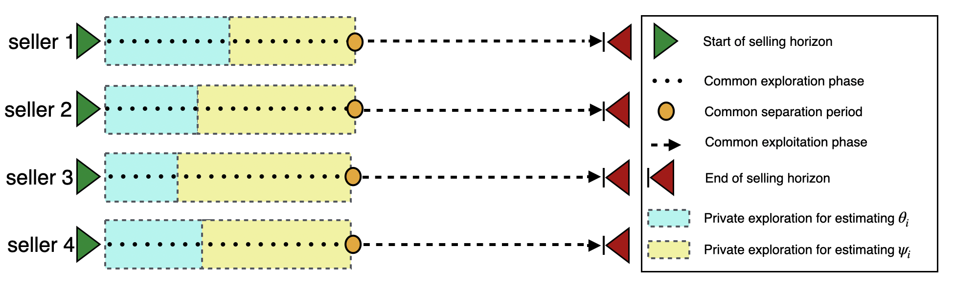
Figure 1: Illustration of our policy (Algorithm˜1) with $N=4$ sellers in sequential price competition under nonlinear demands. For each seller $i\in\{1,2,3,4\}$, in their exploration phase (dotted line) of length $\tau$, they offer randomized prices following their distribution $\mathscr{D}_{i}$. Within the exploration phase, each seller has a private phase for estimating $\theta_{i}$ (blue box), with length $\tau\kappa_{i}$ and a private phase for estimating $\psi_{i}$ (yellow box), with length $\tau(1-\kappa_{i})$. The seller’s price experiment ends at period $t=\tau$ (orange circle). Subsequently, in their exploitation phase (dashed line), seller $i$ offers prices using the estimators generated in the exploration phase.

1. Exploration phase part 1: $\mathcal{T}_{i}^{(1)}$. In this first part of the exploration phase, seller $i$ considers the estimator

   $$(\widetilde{\beta}_{i},\widetilde{\bm{\gamma}}_{i})=\widetilde{\theta}_{i}\triangleq\widehat{\theta}_{i}/\|\widehat{\theta}_{i}\|_{2},$$

   where

   $$\textstyle\widehat{\theta}_{i}=\operatorname{argmin}_{\theta\in\mathbb{R}^{N}}\mathscr{L}_{i}(\theta),\quad\mathscr{L}_{i}(\theta)\triangleq\sum_{t\in\mathcal{T}_{i}^{(1)}}(y_{i}^{(t)}-\theta^{\top}(\mathbf{p}^{(t)}-\bar{\mathbf{p}}))^{2},\quad\bar{\mathbf{p}}=\frac{1}{|\mathcal{T}_{i}^{(1)}|}\sum_{t\in\mathcal{T}_{i}^{(1)}}\mathbf{p}^{(t)}.$$ (8)

   The linear estimator $\widehat{\theta}_{i}$ goes back to Brillinger (2012) and it is exactly what one would use if the regression model were known to be linear.

2. Exploration phase part 2: $\mathcal{T}_{i}^{(2)}$. For the second part define $w^{(t)}_{i}\triangleq\widetilde{\theta}_{i}^{\top}\textbf{p}^{(t)}$ for $t\in\mathcal{T}_{i}^{(2)}$, and define the estimator:

   $$\textstyle\widehat{\psi}_{i,\widetilde{\theta}_{i}}\in\operatorname{argmin}_{\psi\in\mathcal{H}_{i}}\sum_{t\in\mathcal{T}_{i}^{(2)}}(y_{i}^{(t)}-\psi(w^{(t)}_{i}))^{2},$$ (9)

   where $\mathcal{H}_{i}$ is the class of $(c_{i}-1)$-concave functions $\psi:\mathcal{U}\rightarrow\mathbb{R}$, where $\mathcal{U}$ is defined in Equation˜4.

During the exploitation phase, every firm will obtain an estimated revenue function by plugging in its estimators from the exploration phase:

$$\widehat{\operatorname{rev}}_{i}(p_{i}|\mathbf{p}_{-i}^{(t-1)})\triangleq\widehat{\psi}_{i,\widetilde{\theta}_{i}}(-\widetilde{\beta}_{i}p_{i}+\widetilde{\bm{\gamma}}_{i}^{\top}\mathbf{p}_{-i}^{(t-1)}),$$ (10)

where $\mathbf{p}_{-i}^{(t-1)}$ are the prices of all the other firms at time $t-1$, that are made public. A price $p^{(t)}_{i}$ is then offered by firm $i$ as a maximizer of Equation˜10. We present the full algorithm in Algorithm˜1 and a scheme in Figure˜1.

Algorithm 1 SPE-BR (Semi-Parametric Estimation then Best-Response)

Input: the proportion $\xi\in(0,1)$ of time horizon corresponding to the exploration phase lengths $\tau\propto T^{\xi}\in\mathbb{N}$; the (joint) distributions of the exploration phase $\mathscr{D}$; $\kappa_{i}$ for $i\in\mathcal{N}$ the proportion of exploration phase used to estimate $\theta_{i}$.

Output: Price $p_{i}^{(t)}$ that seller $i\in\mathcal{N}$ offers in period $t\in\mathcal{T}$.

for $t=1,2,\dots,T$ do

  Sample i.i.d. $(\tilde{p}_{1}^{(t)},\tilde{p}_{2}^{(t)},\dots,\tilde{p}_{N}^{(t)})=\tilde{\mathbf{p}}^{(t)}\sim\mathscr{D}$.

  Each seller $i\in\mathcal{N}$ offers a price

$$p_{i}^{(t)}=\tilde{p}_{i}^{(t)}\mathbf{1}\{t\leq\tau\}+\mathbf{1}\{t>\tau\}\cdot\operatorname{argmax}_{p_{i}\in\mathcal{P}_{i}}\,p_{i}\widehat{\psi}_{i,\widetilde{\theta}_{i}}(-\widetilde{\beta}_{i}p_{i}+\widetilde{\bm{\gamma}}_{i}^{\top}\mathbf{p}_{-i}^{(t-1)}).$$

  Each seller $i\in\mathcal{N}$ observes individual realized demand $y_{i}^{(t)}$.

  When $t=\tau$, each seller $i\in\mathcal{N}$ construct an estimator $(\widetilde{\theta}_{i},\widehat{\psi}_{i,\widetilde{\theta}_{i}}(\cdot))$ using data $\{(\mathbf{p}^{(t)},y_{i}^{(t)})\}_{t=1,2,\ldots,\tau}$ as defined in Equation˜8 and Equation˜9.

end for

Remark 5.1 (The common exploration phase).

To highlight the importance of a common exploration phase, we demonstrate that no seller has an incentive to extend or shorten the exploration phase. If firm $i$ prolongs its exploration phase, it risks incomplete learning of its model parameters (Keskin & Zeevi, 2018), leading to inaccurate parameter estimation and, consequently, a loss in revenue. Conversely, if firm $i$ shortens its exploration phase, it may achieve consistent estimation but at the cost of higher regret due to insufficient exploratory data. For a better illustration, consider a scenario where firm $i$ extends its exploration phase to $\tau^{\prime}>\tau$ while all other firms use a phase of length $\tau$. When firm $i$ estimates its parameters using data $\{(\mathbf{p}^{(t)},y_{i}^{(t)})\}_{t\leq\tau^{\prime}}$, the data from times $\tau+1$ to $\tau^{\prime}$ are no longer iid. In this later period, all other firms have already started their exploration, causing the prices $\{\mathbf{p}_{-i}^{(t)}\}_{t=\tau+1,\dots,\tau^{\prime}}$ to be dependent on the earlier data $\{\mathbf{p}_{-i}^{(t)}\}_{t\leq\tau}$. This dependency can result in inconsistent parameter estimation and a loss of efficiency for firm $i$. Conversely, if firm $i$ opts for a shorter exploration phase than $\tau$, it may achieve consistent estimation, but the reduced amount of exploratory data could lead to lower efficiency compared to firms that adhere to the full exploration phase.

Remark 5.2 (Need for two different phases for model estimation).

In principle, one could estimate $(\theta_{i},\psi_{i})$ jointly using the full exploration phase. For instance, Balabdaoui et al. (2019) employ a profile least squares approach to achieve $L^{2}$ convergence for the joint LSE of $(\theta_{i},\psi_{i})$ based on the data $\{(y_{i}^{(t)},\mathbf{p}^{(t)})\}_{t\leq\tau}$. However, in our context, $L^{2}$ convergence alone does not suffice to establish an upper bound on the total expected regret. To elaborate, let $(\theta_{i}^{JLS},\psi_{i}^{JLS})$ denote the joint estimator proposed in Balabdaoui et al. (2019) based on the data $\{(y_{i}^{(t)},\mathbf{p}^{(t)})\}_{t\leq\tau}$. Their result applied to our setting gives the following $L^{2}$ convergence rate:

$$\left(\int_{\mathcal{P}}\left(\psi_{i}^{JLS}(\mathbf{p}^{\top}\theta_{i}^{JLS})-\psi_{i}(\mathbf{p}^{\top}\theta_{i})\right)^{2}d\mathscr{D}(\mathbf{p})\right)^{1/2}=O_{p}\left(\tau^{-1/3}\right).$$

Here, the convergence is measured with respect to the measure $\mathscr{D}$, which governs the distribution of prices during the exploration phase. Consequently, the $L^{2}$ distance between $(\theta_{i},\psi_{i})$ and $(\theta_{i}^{JLS},\psi_{i}^{JLS})$ can only be evaluated for prices distributed according to $\mathscr{D}$. This is problematic because, in the exploitation phase ($t\geq\tau+1$), the distribution of prices $\mathbf{p}^{(t)}$ may differ from $\mathscr{D}$. A uniform convergence result, which does not depend on any specific price distribution, is critical to our problem. However, achieving uniform convergence of the form

$$\sup_{\mathbf{p}\in\mathcal{P}}\left|\psi_{i}^{JLS}(\mathbf{p}^{\top}\theta_{i}^{JLS})-\psi_{i}(\mathbf{p}^{\top}\theta_{i})\right|$$ (11)

is challenging when $(\theta_{i}^{JLS},\psi_{i}^{JLS})$ are estimated jointly. To overcome this difficulty, our approach is to first estimate $\theta_{i}$ and then, conditional on this estimator, separately estimate $\psi_{i}$ using an independent dataset. This two-step procedure ensures conditional independence and yields consistent estimators, addressing the difficulties of the joint estimation strategy.

6 Convergence of NE and Regret Analysis

We first analyze, for every seller $i\in\mathcal{N}$, the convergence of the estimators $\widetilde{\theta}_{i}$ in Section˜6.1 and $\widehat{\psi}_{i,\widetilde{\theta}_{i}}$ in Section˜6.2, associated with the exploration phase. Then we analyze the convergence of the NE and the upper bound on the total regret in Section˜6.3.

6.1 Estimation of the Parametric Component

In a single-index model, the linear estimator in Equation˜8 converges to the true $\theta_{i}$ at a $\sqrt{n}$ rate and is asymptotically Gaussian (Chmielewski, 1981), provided that the covariates (in this case, the joint prices $\mathbf{p}^{(t)}$) follow an elliptical distribution (Balabdaoui et al., 2019; Brillinger, 2012). We adopt the same elliptical assumption to ensure the consistency of the estimator in Equation˜8. More specifically, and in contrast to earlier work, we establish a concentration inequality for this estimator (Proposition˜6.3), which serves as a key tool in deriving our regret upper bound.

We assume that in the exploration phase the distribution $\mathscr{D}$ of the covariates is elliptically symmetric with density generator $g$ supported on $[0,\infty)$, location vector $\mathbf{m}\in\mathbb{R}^{N}$, and a positive definite scale matrix $\Lambda$, i.e.

$$f_{\mathbf{p}}(\mathbf{p})\propto\,g((\mathbf{p}-\mathbf{m})^{T}\Lambda^{-1}(\mathbf{p}-\mathbf{m})),$$

and we denote the above distribution by $\mathscr{D}=\mathscr{E}(\mathbf{m},\Lambda,g)$. We denote $\operatorname{var}(\mathbf{p})$ by $\Sigma$, which is proportional to $\Lambda$.

Remark 6.1.

It should be noted that from a purely theoretical stand-point we do not restrict the domain of the price vector in the exploration phase to $\mathcal{P}$, but this has essentially no implication for the application of the pricing algorithm in practice. To ensure that the $i$’th seller’s exploration prices can, realistically, never lie outside $\mathcal{P}_{i}=[\underline{p_{i}},\bar{p}_{i}]$, all they need is to take $\mathscr{D}_{i}$ be a normal distribution (for example) centered at the midpoint of this interval with variance $\sigma_{i}^{2}$ taken to be an adequately small fraction of the length of $\mathcal{P}_{i}$. If the sellers function independently, as is generally the case, the joint distribution is certainly elliptically symmetric. More generally, view the parameters $\Lambda$, $\mathbf{m}$, and $g$ as concentrating the mass of $\mathscr{D}$ in $\mathcal{P}$ with overwhelmingly high probability. Theoretically, some proposed price in many thousands of time steps could lie outside $\mathcal{P}$, but realistically the procedure entails no financial consequence for them. Letting $\mathscr{D}$ belong to an infinitely supported elliptical distribution allows the implementation of a simple linear regression-based approach to learn $\theta_{i}$ which satisfies the useful concentration inequality proved in Proposition 6.3 below, and is also important for certain conditioning arguments involved in estimating appropriate surrogates for $\psi_{i}$ in the following subsection, while compromising nothing in terms of the core conceptual underpinnings of the problem.

Assumption 6.2.

$\mathscr{D}=\mathscr{E}(\mathbf{m},\Lambda,g)$, where $c_{\min}\mathbb{I}\preccurlyeq\Lambda\preccurlyeq c_{\max}\mathbb{I}$ for some $0<c_{\min}<c_{\max}<\infty$ and the density generator $g$ is such that $g(x+y)=g(x)g(y)$ for all $x,y\geq 0$.

˜6.2 holds for a wide range of distributions, including Gaussian distributions and, more generally, all elliptically symmetric distributions for which $g(x)=a^{-\gamma x}$, for $a>0$ and $\gamma>0$. This assumption on $g$ is instrumental in estimating $\theta_{i}$ since it guarantees that the sampled points are sub-Gaussian, a property that is essential for deriving the concentration inequality in Proposition˜6.3. Moreover, as we will discuss in Section˜6.2, this assumption is also beneficial for the estimation of $\psi_{i}$ because it ensures that $\psi_{i,\theta}(u)$ (defined in Equation˜12) depends on $u$ solely through the argument of $\psi_{i}$ rather than that of $g$, and this decoupling guarantees that $\psi_{i,\theta}$ inherits key properties from $\psi_{i}$, such as smoothness and adherence to the prescribed shape constraints, as highlighted in Proposition˜6.5.

Since the covariance matrix of an elliptically symmetric distribution $\mathscr{E}(\mathbf{m},\Lambda,g)$ is proportional to $\Lambda$, then there exists $0<\varsigma_{\min}<\infty$ such that $\varsigma_{\min}\preccurlyeq\Sigma$, where $\Sigma=\operatorname{var}(\mathbf{p})$, $\mathbf{p}\sim\mathscr{E}(\mathbf{m},\Lambda,g)$. These constant will appear in Proposition˜6.3, which proof is provided in Appendix˜C.

Proposition 6.3.

Under ˜6.2, there exist positive constants $c$ and $C$ (that depend solely on $(\theta_{i},\psi_{i})$ and the variance proxies of the sub-Gaussian random variables $y_{i}^{(t)}$ and $\mathbf{p}^{(t)}$) such that, for $n_{i}^{(1)}$ sufficiently large, with probability at least $1-2e^{-c\varsigma_{\min}^{2}n_{i}^{(1)}/16}-\nicefrac{{2}}{{n_{i}^{(1)}}}$, the estimator in Equation˜8 satisfies

$$\|\widetilde{\theta}_{i}-\theta_{i}\|_{2}\leq C\sqrt{\tfrac{N\log n_{i}^{(1)}}{n_{i}^{(1)}}}.$$

6.2 Estimation of the Link Function via s-Concavity

This section provides a uniform convergence result of $\widehat{\psi}_{i,\theta}$ to $\psi_{i}$ for any fixed $\theta\in\mathbb{S}_{N-1}$. In this section, all the results must be considered as conditioned on $\theta=\widetilde{\theta}_{i}$ estimated using data in $\mathcal{T}_{i}^{(1)}$ independent of data in $\mathcal{T}_{i}^{(2)}$. For simplicity of notation, we re-index $\mathcal{T}_{i}^{(2)}$ as $[n]=\{1,2,\dots,n\}$. To estimate $\psi_{i}$ we would need to know $\theta_{i}$ in advance, indeed we remind that $\mathbb{E}(y^{(t)}_{i}\mid\mathbf{p}^{(t)})=\psi_{i}(\theta_{i}^{\top}\mathbf{p}^{(t)})$. However, our knowledge is limited to an approximation $\theta$ of $\theta_{i}$, and the observable design points are $w^{(t)}_{i}\triangleq\theta^{\top}\mathbf{p}^{(t)}$. This implies that, with data $\{(w^{(t)}_{i},y^{(t)}_{i})\}_{t\in[n]}$, we are only able to estimate

$$\psi_{i,\theta}(u)\triangleq\mathbb{E}(y^{(t)}_{i}\mid w^{(t)}_{i}=u),\quad u\in\mathbb{R}.$$ (12)

We will now construct an estimator of $\psi_{i,\theta}$, and we will prove, in Theorem˜6.6, a uniform convergence result in the (bounded) set $\mathcal{U}\subset\mathbb{R}$ (where $\mathcal{U}$ defined on Equation˜4), however, the result holds for any bounded set $K\subset\mathbb{R}$. Indeed, from Mösching & Dümbgen (2020) we have that if the density of the design points $f_{w}$ is bounded away from $0$ on a set $U$, then $\{w^{(t)}_{i}\}_{t\in[n]}$ are “asymptotically dense” within each interval contained in $U$, which condition is sufficient to produce a uniform convergence result of our estimator of $\psi_{i,\theta}$ on any interval contained in $U$. In our case, $f_{w}$ is supported on all $\mathbb{R}$, and hence $f_{w}$ is bounded away from $0$ on any bounded set $K$, therefore the convergence result holds uniformly on any bounded set $K\subset\mathbb{R}$.

Remark 6.4.

Note that, since the NE $\mathbf{p}^{*}$ falls in the interior of $\mathcal{P}$, our algorithm will be able to converge to it if $\epsilon$ is sufficiently small to guarantee $\theta_{i}^{\top}\mathbf{p}^{*}\in\operatorname{int}(\mathcal{U})$ for all $i\in\mathcal{N}$.

A closed-form expression for $\psi_{i,\theta}(\cdot)$ and some of its properties are proved in Proposition˜6.5.

Proposition 6.5.

Under ˜4.1 and ˜6.2 we have the following properties:

1. $\psi_{i,\theta}(u)=\int_{\mathbb{R}^{N-1}}\psi_{i}\left(\theta_{i}^{\top}\mathbf{m}_{u}+\theta_{i}^{\top}A\bm{\alpha}\right)\tilde{g}(\bm{\alpha})d\bm{\alpha}$, $u\in\mathbb{R}$, $\theta\in\mathbb{S}_{N-1}$, where $\tilde{g}(\bm{\alpha})=\nicefrac{{g(\|\bm{\alpha}\|_{2}^{2})}}{{\int_{\mathbb{R}^{N-1}}g(\|\bm{\alpha}\|_{2}^{2})d\bm{\alpha}}}$ is independent of $u$, $\mathbf{m}_{u}$ is defined in Equation˜21, and $A$ is such that $AA^{\top}=\Lambda$.

2. $\psi_{i,\theta}$ is bounded uniformly in $\theta\in\mathbb{S}_{N-1}$.

3. $\psi_{i,\theta}\in\mathrm{C}^{2}(\mathcal{U})$ and $|\psi_{i,\theta}|$ is bounded from above uniformly in $\theta\in\mathbb{S}_{N-1}$.

4. $|\psi_{i}(u)-\psi_{i,\theta}(u)|\lesssim\|\theta-\theta_{i}\|_{2}$ for all $u\in\mathcal{U}$ and $\theta\in\mathbb{S}_{N-1}$.

5. If also ˜4.2 holds (i.e. $\psi_{i}$ is $s_{i}$-concave for some $s_{i}>-1$ as it arises from Proposition˜4.3) then $\psi_{i,\theta}$ is $s_{i}$-concave for any $\theta\in\mathbb{S}_{N-1}$.

Proposition˜6.5 is crucial because it tells us that if we had a (uniform) consistent estimate $\widehat{\psi}_{i,\theta}(u)$ of $\psi_{i,\theta}(u)$, then by point (4), $\widehat{\psi}_{i,\theta}(u)$ is close to $\psi_{i}$ as long as $\theta$ is close to $\theta_{i}$, which will be used to prove the regret upper bound. Moreover, guided by point (5) in Proposition˜6.5 we estimate $\psi_{i,\theta}(u)$ using LSE under $s_{i}$-concavity restriction, denoted as

$$\widehat{\phi}_{i,\theta}\triangleq\operatorname{argmin}_{\phi\in\mathcal{S}}\sum_{t\in[n]}(y_{i}^{(t)}-h_{s_{i}}\circ\phi(w_{i}^{(t)}))^{2},$$ (13)

where $\mathcal{S}$ is the set of concave functions $\phi:\mathcal{U}\rightarrow\mathbb{R}$. We are now prepared to demonstrate the convergence of $\widehat{\psi}_{i,\theta}$ to $\psi_{i,\theta}$, where

$$\widehat{\psi}_{i,\theta}\triangleq h_{s_{i}}\circ\widehat{\phi}_{i,\theta}.$$

Theorem 6.6.

Let ˜6.2 and ˜4.2 hold. Then, by Proposition˜4.3 and Proposition˜6.5, $\psi_{i,\theta}$ is $s_{i}$-concave for some $s_{i}>-1$. Let $m=\pi n$, where $\pi=\int_{\mathcal{U}}f_{w}(u)du$ is the proportion of data points $\{w_{i}^{(t)}\}_{t\in[n]}$ lying in the set $\mathcal{U}$ as $n\rightarrow\infty$. For every $\gamma>2$ there exists $m_{0}$, a constant $\kappa>0$ and $C>0$ depending only on constants in the assumptions such that

$$\mathbb{P}\left\{\sup_{\theta\in\mathbb{S}_{N-1}}\sup_{u\in\mathcal{U}_{m}}|\widehat{\psi}_{i,\theta}(u)-\psi_{i,\theta}(u)|\leq\kappa(\nicefrac{{\log(m)}}{{m}})^{2/5}\right\}\geq 1-\nicefrac{{1}}{{m^{\gamma-2}}},\quad m\geq m_{0},$$

where $\mathcal{U}_{m}=\{u\in\mathcal{U}:\left[u\pm\delta_{m}\right]\subset\mathcal{U}\}$, with $\delta_{m}=C(\nicefrac{{\log(m)}}{{m}})^{1/5}$.

Theorem˜6.6 is an application of our more general Theorem˜F.5 (and following Remark˜F.6). We defer to Appendix˜G for the proof.

6.3 NE and Regret

Recall that $\operatorname{rev}_{i}(p\mid\mathbf{p}_{-i})=p\psi_{i}(-\beta_{i}p+\bm{\gamma}_{i}^{\top}\mathbf{p}_{-i})$. Before stating our main theorem, we need the following assumption.

Assumption 6.7.

There exists $\mu_{i}>0$ such that $\operatorname{rev}_{i}(\Gamma_{i}(\mathbf{p})\mid\mathbf{p}_{-i})-\operatorname{rev}_{i}(q\mid\mathbf{p}_{-i})\geq\mu_{i}(\Gamma_{i}(\mathbf{p})-q)^{2}$ for all $\mathbf{p}=(p_{i},\mathbf{p}_{-i})\in\mathcal{P}$ and $q\in\mathcal{P}_{i}$.

Remark 6.8.

˜6.7 informally states that the revenue functions are smooth around the NE. ˜6.7 is satisfied in several scenarios, for example when $-\partial^{2}_{p^{2}}\operatorname{rev}_{i}(p\mid\mathbf{p}_{-i})\geq L$ for all $p\in\mathcal{P}_{i}$ for some $L>0$ independent of $\mathbf{p}_{-i}$. Indeed, in this case, since $\partial_{p}\operatorname{rev}_{i}(\Gamma_{i}(\mathbf{p})\mid\mathbf{p}_{-i})=0$ we have that $\operatorname{rev}_{i}(\Gamma_{i}(\mathbf{p})\mid\mathbf{p}_{-i})-\operatorname{rev}_{i}(p_{i}\mid\mathbf{p}_{-i})\geq L(p_{i}-\Gamma_{i}(\mathbf{p}))^{2}/2$. Examples where the condition $-\partial^{2}_{p^{2}}\operatorname{rev}_{i}(p\mid\mathbf{p}_{-i})\geq L$ for all $p\in\mathcal{P}_{i}$ for some $L>0$ independent of $\mathbf{p}_{-i}$ is satisfied are: the linear demand models (Li et al., 2024), the concave demand models, and the $s_{i}$-concave demand functions for some $s_{i}>-1$. For a more detailed description of these and more examples, we defer to Appendix˜H.

In Theorem˜6.9, we present our main result for a fixed value $\xi\in(0,1)$, which, we recall, represents the proportion of (common) exploration length $\tau\propto T^{\xi}$.

Theorem 6.9.

Suppose that ˜4.1, ˜4.2, ˜4.4, ˜6.2 and ˜6.7 hold. Then, Algorithm˜1 produces a policy such that, for each $i\in\mathcal{N}$:

1. Individual sub-linear regret: $\operatorname{Reg}_{i}(T)=O(T^{\xi}+T^{1-\nicefrac{{2\xi}}{{5}}}N^{\nicefrac{{1}}{{2}}}(\log T)^{\nicefrac{{2}}{{5}}})$.

2. Convergence to NE: $\mathbb{E}\left[\|\mathbf{p}^{(T)}-\mathbf{p}^{*}\|_{2}^{2}\right]=O(N^{\nicefrac{{1}}{{2}}}T^{-\nicefrac{{2\xi}}{{5}}}(\log T)^{\nicefrac{{2}}{{5}}})$. More precisely, we have

   $$\mathbb{E}\left[\|\mathbf{p}^{(t)}-\mathbf{p}^{*}\|_{2}^{2}\right]\lesssim N^{\nicefrac{{1}}{{2}}}T^{-\nicefrac{{2\xi}}{{5}}}(\log T)^{\nicefrac{{2}}{{5}}}+L^{2(t-\tau-1)}_{\bm{\Gamma}},\quad t\geq\tau+1.$$

In Corollary˜6.10, we provide the exploration-exploitation trade off for our Algorithm˜1. More specifically, we provide the optimal choice of $\xi$ that minimizes the expected regrets. Corollary˜6.10 follows immediately from Theorem˜6.9 by equalizing the exponents of $T$ in the regret upper bound (ignoring logarithmic factors)

$$T^{\xi}+T^{1-\nicefrac{{2\xi}}{{5}}},$$

which yields the value of $\xi=5/7$ that minimizes the total expected regret.

Corollary 6.10.

Suppose that the same assumption in Theorem˜6.9 holds. Then, the value of $\xi\in(0,1)$ that minimizes the expected regrets is $\xi=5/7$. With this choice, we get that for each $i\in\mathcal{N}$:

1. Individual sub-linear regret: $\operatorname{Reg}_{i}(T)=O(N^{\nicefrac{{1}}{{2}}}T^{\nicefrac{{5}}{{7}}}(\log T)^{\nicefrac{{2}}{{5}}})$.

2. Convergence to NE: $\mathbb{E}\left[\|\mathbf{p}^{(T)}-\mathbf{p}^{*}\|_{2}^{2}\right]=O(N^{\nicefrac{{1}}{{2}}}T^{-\nicefrac{{2}}{{7}}}(\log T)^{\nicefrac{{2}}{{5}}})$.

7 Numerical Experiments

We test the performance of our Algorithm˜1 in the sequential price competition with $N\in\{2,5,8\}$ sellers. For each seller $i\in\mathcal{N}=\{1,2,\dots,N\}$, the price is supported on $\mathcal{P}=[0,3]^{\times N}$. The link functions are defined as $\psi_{i}(u)=\Phi(u-i+1)$ where $\Phi$ is the cumulative distribution function of a standard Gaussian random variable which is log-concave and therefore $0$-concave. Their price sensitivities $\beta_{i}=[0.71,0.915,0.97]$ and $\gamma_{ij}=\sqrt{(1-\beta_{i}^{2})/(N-1)}$ are such that $\theta_{i}=(\beta_{i},\bm{\gamma}_{i})$ has unitary $L^{2}$-norm and satisfy ˜4.4, because, by Remark˜4.6, $\|\bm{\gamma}_{i}\|_{1}<\nicefrac{{1}}{{\sqrt{2}}}$. A fixed point exists and is unique by Lemma˜4.5 and is evaluated using Picard’s iteration, and we check that the fixed point falls in the interior of $\mathcal{P}$. The demand noise of firm $i$ follows a uniform distribution on $[-0.0.3,0.0.3]$. For every $T\in[100,200,400,800,1600]$, we apply Algorithm˜1. We independently repeat the simulation $35$ times to obtain average performances and $95\%$ of confidence intervals. In Figure˜2 we report the results: we display the convergence of the estimators $\theta_{i}$ and $\psi_{i}$, as well as the convergence to the Nash equilibrium $\mathbf{p}^{*}$, and the expected cumulative regret.

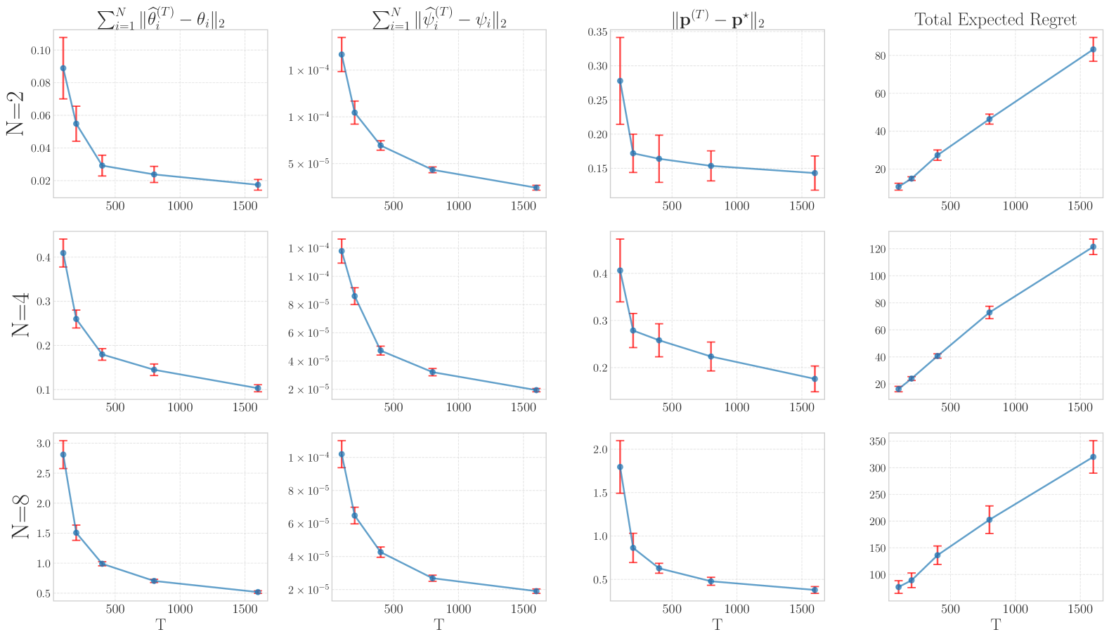
Figure 2: Performance of Algorithm 1 in sequential price competition with $N\in\{2,4,8\}$ sellers.

8 Conclusions

In this paper, we introduced an innovative online learning algorithm for sequential price competition, where each seller’s mean demand is modeled as a nonlinear function of joint prices. This departure from standard parametric models (Li et al. (2024); Kachani et al. (2007); Gallego et al. (2006)) not only broadens the scope of demand modeling but also enhances the realism of market interactions. Leveraging shape constraints on the mean demand function that arise naturally in the literature, we demonstrated the existence of the NE, provided an upper bound on the algorithm’s regret, and established a convergence rate for the joint prices to the Nash Equilibrium.

Future research directions. There are several promising avenues for further research. One direction is to design an algorithm that permits each seller to independently determine the length of their exploration phase, which is difficult in our setting for reasons elaborated in Remark˜5.1.

On the theoretical front, an important research direction is achieving uniform convergence of the joint estimator $(\theta_{i},\psi_{i})$. While this does not affect the theoretical convergence rate of the regret or the Nash equilibrium – since it influences only a constant factor (given that $\theta_{i}$ is estimated using $\kappa_{i}\tau$ data points and $\psi_{i}$ using $(1-\kappa_{i})\tau$, where $\tau$ is the length of the exploration phase, whereas a joint estimator would treat $\tau$ as a single sample size rather than splitting it) – it may yield practical improvements. Two existing theoretical results are relevant to the joint estimator: Balabdaoui et al. (2019) and Kuchibhotla et al. (2021). The former establishes $L^{2}$ convergence for the joint estimator, which is insufficient for deriving an upper bound on the expected regret. Notably, while Balabdaoui et al. (2019) imposes only a monotonicity constraint on $\psi_{i}$, our framework requires $s_{i}$-concavity to guarantee the existence of an equilibrium. The latter work, Kuchibhotla et al. (2021), provides a uniform convergence result for $(\theta_{i},\psi_{i})$, but under the assumption that $\psi_{i}$ is convex (or concave, i.e., $s_{i}=1$). Moreover, their result offers only an $O_{P}$ rate rather than a concentration inequality, making it insufficient for establishing a regret bound in expectation. Differently from these works, our framework would require a concentration inequality in the supremum norm of the joint estimator, i.e., deriving a probability tail bound of the event in Equation˜11.

Another theoretical challenge lies in estimating the $s_{i}$’s. In this work, we assume $s_{i}$ is known, but in practice, its true value may be uncertain. While our algorithms can be extended to estimating $\psi_{i}$ and $s_{i}$ simultaneously, the theoretical foundations for such an approach are a challenge in their own right and remain to be explored.

Finally, a compelling direction for future exploration is to develop an algorithm that foregoes the traditional exploration-exploitation trade-off. In a more realistic framework, each seller $i$ would utilize all past (public) price observations $\mathbf{p}^{(1)},\mathbf{p}^{(2)},\dots,\mathbf{p}^{(t-1)}$ and corresponding (private) demand data $y_{i}^{(1)},y_{i}^{(2)},\dots,y_{i}^{(t-1)}$ to set the price $p_{i}^{(t)}$ at every time $t$, such that $\mathbf{p}^{(T)}$ converges to the Nash Equilibrium as $T\rightarrow\infty$. A key challenge in this setting is to prevent incomplete learning of the model parameters (Keskin & Zeevi, 2018), which can lead to suboptimal parameter estimates and a consequential loss in revenue, manifested as higher regret.

Acronymous

Acronym	Full Form
NE	Nash Equilibrium
LSE	Least Squares Estimator
NPLSE	Non-Parametric Least Squares Estimator
NPLS	Non-Parametric Least Squares
GLM	Generalized Linear Model
MLE	Maximum Likelihood Estimator
UCB	Upper Confidence Bound
SPE-BR	Semi-Parametric Estimation then Best Response

Table 1: List of Acronyms Used in This Paper

Appendix Contents

• Proof of Proposition˜4.3

• Proof of Lemma˜4.5

• Proof of Proposition˜6.3

• Proof of Proposition˜6.5

• Proof of Theorem˜6.9

• NPLS for s-concave regression

  • Proof of Theorem˜F.5

Appendix A Proof of Proposition˜4.3

$\varphi_{i}^{\prime}=1+\frac{\psi_{i}^{\prime}\cdot\psi_{i}^{\prime}-\psi_{i}\cdot\psi_{i}^{\prime\prime}}{(\psi_{i}^{\prime})^{2}}=2-\frac{\psi_{i}\cdot\psi_{i}^{\prime\prime}}{(\psi_{i}^{\prime})^{2}}\geq c_{i}$ iff $\psi_{i}\cdot\psi_{i}^{\prime\prime}+(\mu-1)(\psi_{i}^{\prime})^{2}\leq 0$ with $\mu=c_{i}-1$. The statement follows by Proposition˜A.1.

Proposition A.1.

Let $\psi:(a,b)\rightarrow(0,\infty)$, a twice differentiable function. Then $\psi$ is $s$-concave iff $\psi\cdot\psi^{\prime\prime}+(s-1)(\psi^{\prime})^{2}\leq 0$ in $(a,b)$.

A.1 Proof of Proposition˜A.1

As for $s=0$ is a known result, we prove it for $s\neq 0$. A function $\psi$ is $s$-concave if and only if $d_{s}\circ\psi$ is concave, where $d_{s}$ is defined in Equation˜3. Then $\psi$ is $s$-concave if and only if

$$\frac{d^{2}}{du^{2}}d_{s}(\psi(u))=\frac{d}{du}\left[|s|\psi^{s-1}(u)\psi^{\prime}(u)\right]=|s|\frac{\psi(u)\psi^{\prime\prime}(u)+(s-1)(\psi^{\prime}(u))^{2}}{\psi^{2-s}(u)}\leq 0,\quad u\in(a,b).$$

Appendix B Proof of Lemma˜4.5

We first find an explicit solution of $\Gamma_{i}(\mathbf{p}^{*})$. We have $\lambda_{i}(\mathbf{p})=\psi_{i}(\theta_{i}(\mathbf{p}))$, where $\theta_{i}(\mathbf{p})=-\beta_{i}p_{i}+\bm{\gamma}_{i}^{\top}\mathbf{p}_{-i}$. By ˜4.2, the first order condition of Equation˜7 is

$$\psi_{i}(\theta_{i}(\mathbf{p}^{*}))-\beta_{i}p_{i}^{*}\psi^{\prime}_{i}(\theta_{i}(\mathbf{p}^{*}))=0 \Leftrightarrow\beta_{i}p_{i}^{*}-\frac{\psi_{i}(\theta_{i}(\mathbf{p}^{*}))}{\psi^{\prime}_{i}(\theta_{i}(\mathbf{p}^{*}))}=0$$

$$\Leftrightarrow\varphi_{i}(\theta_{i}(\mathbf{p}^{*}))=\bm{\gamma}_{i}^{\top}\mathbf{p}^{*}_{-i}$$

$$\Leftrightarrow\theta_{i}(\mathbf{p}^{*})=\varphi_{i}^{-1}(\bm{\gamma}_{i}^{\top}\mathbf{p}^{*}_{-i})$$

$$\Leftrightarrow p^{*}_{i}=\frac{\bm{\gamma}_{i}^{\top}\mathbf{p}^{*}_{-i}-\varphi_{i}^{-1}(\bm{\gamma}_{i}^{\top}\mathbf{p}^{*}_{-i})}{\beta_{i}},$$

or equivalently

$$\Gamma_{i}(\mathbf{p}^{*})\triangleq\frac{g_{i}(\bm{\gamma}_{i}^{\top}\mathbf{p}^{*}_{-i})}{\beta_{i}}.$$ (14)

In other words, $\mathbf{p}^{*}$ are a fixed point for the map $\bm{\Gamma}\triangleq\left(\Gamma_{i}\right)_{i\in\mathcal{N}}$ on the compact space $\mathcal{P}$; i.e., $\bm{\Gamma}\left(\mathbf{p}^{*}\right)=\mathbf{p}^{*}$. To show that Nash equilibrium prices $\mathbf{p}^{*}$ exist and are unique, we only need to prove that $\bm{\Gamma}$ is a contraction mapping. For any $\mathbf{p},\mathbf{p}^{\prime}\in\mathcal{P}$, we have

$$\|\bm{\Gamma}\left(\mathbf{p}\right)-\bm{\Gamma}(\mathbf{p}^{\prime})\|_{\infty} =\sup_{i\in\mathcal{N}}|\Gamma_{i}(\mathbf{p})-\Gamma_{i}(\mathbf{p}^{\prime})|=\sup_{i\in\mathcal{N}}\left|\frac{g_{i}(\bm{\gamma}_{i}^{\top}\mathbf{p}_{-i})-g_{i}(\bm{\gamma}_{i}^{\top}\mathbf{p}_{-i}^{\prime})}{\beta_{i}}\right|$$

$$\leq\sup_{i\in\mathcal{N}}\frac{1}{\beta_{i}}\|g_{i}^{\prime}\|_{\infty}\left|\bm{\gamma}_{i}^{\top}\mathbf{p}_{-i}-\bm{\gamma}_{i}^{\top}\mathbf{p}_{-i}^{\prime}\right|$$

$$\leq\sup_{i\in\mathcal{N}}\frac{1}{\beta_{i}}\|g_{i}^{\prime}\|_{\infty}\|\bm{\gamma}_{i}\|_{1}\|\mathbf{p}_{-i}-\mathbf{p}_{-i}^{\prime}\|_{\infty}$$

$$\leq\|\mathbf{p}-\mathbf{p}^{\prime}\|_{\infty}\sup_{i\in\mathcal{N}}\|g_{i}^{\prime}\|_{\infty}\frac{\|\bm{\gamma}_{i}\|_{1}}{\beta_{i}}$$

$$=L_{\bm{\Gamma}}\|\mathbf{p}-\mathbf{p}^{\prime}\|_{\infty},$$

where

$$L_{\bm{\Gamma}}\triangleq\sup_{i\in\mathcal{N}}\|g_{i}^{\prime}\|_{\infty}\frac{\|\bm{\gamma}_{i}\|_{1}}{\beta_{i}},$$

which is strictly less than $1$ by ˜4.4.

Appendix C Proof of Proposition˜6.3

For simplicity, we redefine $\mathcal{T}_{i}^{(1)}$ as $\{1,2,\dots,n\}$, $\mathbf{x}^{(t)}=\mathbf{p}^{(t)}-\bar{\mathbf{p}}$. The loss function $\mathscr{L}_{i}(\theta)$ is defined as

$$\mathscr{L}_{i}(\theta)=\frac{1}{n}\sum_{t=1}^{n}\left(y_{i}^{(t)}-\theta^{\top}\mathbf{x}^{(t)}\right)^{2}.$$

Then the gradient and Hessian of $\mathscr{L}_{i}(\theta)$ is given by

$$\nabla_{\theta}\mathscr{L}_{i}(\theta) =\frac{1}{n}\sum_{t=1}^{n}2\left(\theta^{\top}\mathbf{x}^{(t)}-y^{(t)}_{i}\right)\mathbf{x}^{(t)},$$

$$\nabla_{\theta}^{2}\mathscr{L}_{i}(\theta) =\nabla_{\theta}^{2}\mathscr{L}_{i}=\frac{1}{n}\sum_{t=1}^{n}2\mathbf{x}^{(t)}\mathbf{x}^{(t)\top}.$$

Let $\widehat{\theta}_{i}$ be the global minimizer of $\mathscr{L}_{i}(\theta)$. We do a Taylor expansion of $\mathscr{L}_{i}(\widehat{\theta}_{i})$ around $\lambda_{i}\theta_{i}$, with $\lambda_{i}$ to be determined:

$$\mathscr{L}_{i}(\widehat{\theta}_{i})-\mathscr{L}_{i}\left(\lambda_{i}\theta_{i}\right)=\left\langle\nabla\mathscr{L}_{i}\left(\lambda_{i}\theta_{i}\right),\widehat{\theta}_{i}-\lambda_{i}\theta_{i}\right\rangle+\frac{1}{2}\left\langle\widehat{\theta}_{i}-\lambda_{i}\theta_{i},\nabla_{\theta}^{2}\mathscr{L}_{i}\cdot(\widehat{\theta}_{i}-\lambda_{i}\theta_{i})\right\rangle.$$

As $\widehat{\theta}_{i}$ is the global minimizer of loss $\mathscr{L}_{i}(\theta)$, we have $\mathscr{L}_{i}(\widehat{\theta}_{i})\leq\mathscr{L}_{i}\left(\lambda_{i}\theta_{i}\right)$, that is

$$\left\langle\nabla\mathscr{L}_{i}\left(\lambda_{i}\theta_{i}\right),\widehat{\theta}_{i}-\lambda_{i}\theta_{i}\right\rangle+\frac{1}{2}\left\langle\widehat{\theta}_{i}-\lambda_{i}\theta_{i},\nabla_{\theta}^{2}\mathscr{L}_{i}\cdot(\widehat{\theta}_{i}-\lambda_{i}\theta_{i})\right\rangle\leq 0,$$

which implies

$$\left\langle\widehat{\theta}_{i}-\lambda_{i}\theta_{i},\frac{1}{n}\sum_{t=1}^{n}\mathbf{x}^{(t)}\mathbf{x}^{(t)\top}(\widehat{\theta}_{i}-\lambda_{i}\theta_{i})\right\rangle \leq\left\langle\nabla_{\theta}\mathscr{L}_{i}\left(\lambda_{i}\theta_{i}\right),\lambda_{i}\theta_{i}-\widehat{\theta}_{i}\right\rangle$$

$$\leq\left\|\nabla_{\theta}\mathscr{L}_{i}\left(\lambda_{i}\theta_{i}\right)\right\|_{2}\|\lambda_{i}\theta_{i}-\widehat{\theta}_{i}\|_{2}$$

$$\leq\sqrt{N}\left\|\nabla_{\theta}\mathscr{L}_{i}\left(\lambda_{i}\theta_{i}\right)\right\|_{\infty}\|\lambda_{i}\theta_{i}-\widehat{\theta}_{i}\|_{2}.$$

By Lemma˜C.1, the LHS satisfies

$$\left\langle\widehat{\theta}_{i}-\lambda_{i}\theta_{i},\frac{1}{n}\sum_{t=1}^{n}\mathbf{x}^{(t)}\mathbf{x}^{(t)\top}(\widehat{\theta}_{i}-\lambda_{i}\theta_{i})\right\rangle\geq\frac{\varsigma_{\min}}{2}\|\lambda_{i}\theta_{i}-\widehat{\theta}_{i}\|_{2}^{2},$$

w.p. at least $1-2e^{-c\varsigma_{\min}^{2}n/16}$ (as long as $n\geq N16C^{2}/\varsigma_{\min}$) for certain constants $c>0$ and $C>0$ that depend only on the variance proxy of the sub-Gaussian random variable $\mathbf{x}^{(t)}$ and, and by Lemma˜C.2 the RHS satisfies

$$\sqrt{N}\left\|\nabla_{\theta}\mathscr{L}_{i}\left(\lambda_{i}\theta_{i}\right)\right\|_{\infty}\|\lambda_{i}\theta_{i}-\widehat{\theta}_{i}\|_{2}\leq\mathscr{C}\sqrt{\frac{N\log n}{n}}\|\lambda_{i}\theta_{i}-\widehat{\theta}_{i}\|_{2},$$

with probability at least $1-\frac{2N}{n}$ (as long as $n\geq N$), where $\mathscr{C}$ is a constant that depends solely on $\lambda_{i}$ and the variance proxies of the sub-Gaussian random variables $y_{i}^{(t)}$ and $\mathbf{x}^{(t)}$. Putting the two inequalities together we get with probability at least $1-2e^{-c\varsigma_{\min}^{2}n/16}-\tfrac{2N}{n}$ that, for $n$ sufficiently large

$$\|\lambda_{i}\theta_{i}-\widehat{\theta}_{i}\|_{2}\leq C_{1}\sqrt{\frac{N\log n}{n}},$$

where $C_{1}=2\frac{\mathscr{C}}{\varsigma_{\min}}$. Now we conclude. Recall that from Equation˜15 we have that $\lambda_{i}\triangleq\frac{\operatorname{cov}\left(\psi_{i}(\theta_{i}^{\top}\mathbf{x}^{(t)}),\theta_{i}^{\top}\mathbf{x}^{(t)}\right)}{\operatorname{var}(\theta_{i}^{\top}\mathbf{x}^{(t)})}>0$. Let

$$\mathcal{W}_{n}=\left\{\theta:\|\lambda_{i}\theta_{i}-\theta\|_{2}\leq C_{1}\sqrt{\frac{N\log n}{n}}\right\}.$$

Let $n$ be large enough so that $C_{1}\sqrt{\frac{N\log n}{n}}\leq\lambda_{i}$: this guarantees that any $\theta\in\mathcal{W}_{n}$ is such that $\|\theta\|_{2}\neq 0$, which come from the fact that $\|\lambda_{i}\theta_{i}\|_{2}=\lambda_{i}$. Then for $\widehat{\theta}_{i}\in\mathcal{W}_{n}$ we can write

$$\|\theta_{i}-\widetilde{\theta}_{i}\|_{2}=\left\|\theta_{i}-\frac{\widehat{\theta}_{i}}{\|\widehat{\theta}_{i}\|_{2}}\right\|_{2} =\left\|\frac{\lambda_{i}\theta_{i}}{\lambda_{i}}-\frac{\widehat{\theta}_{i}}{\|\widehat{\theta}_{i}\|_{2}}\right\|_{2}$$

$$\lesssim\left\|\frac{\lambda_{i}\theta_{i}-\widehat{\theta}_{i}}{\lambda_{i}}\right\|_{2}+\left\|\widehat{\theta}_{i}\left(\frac{1}{\lambda_{i}}-\frac{1}{\|\widehat{\theta}_{i}\|_{2}}\right)\right\|_{2}$$

$$\lesssim\frac{\|\lambda_{i}\theta_{i}-\widehat{\theta}_{i}\|_{2}}{\lambda_{i}}+\|\widehat{\theta}_{i}\|_{2}\left|\frac{1}{\lambda_{i}}-\frac{1}{\|\widehat{\theta}_{i}\|_{2}}\right|$$

$$=\frac{\|\lambda_{i}\theta_{i}-\widehat{\theta}_{i}\|_{2}}{\lambda_{i}}+\|\widehat{\theta}_{i}\|_{2}\left|\frac{\lambda_{i}-\|\widehat{\theta}_{i}\|_{2}}{\|\widehat{\theta}_{i}\|_{2}\lambda_{i}}\right|$$

$$=\frac{\|\lambda_{i}\theta_{i}-\widehat{\theta}_{i}\|_{2}}{\lambda_{i}}+\frac{|\|\lambda_{i}\theta_{i}\|_{2}-\|\widehat{\theta}_{i}\|_{2}|}{\lambda_{i}}$$

$$\leq 2\frac{\|\lambda_{i}\theta_{i}-\widehat{\theta}_{i}\|_{2}}{\lambda_{i}},$$

and, as $\widehat{\theta}_{i}\in\mathcal{W}_{n}$ with probability at least $1-2e^{-c\varsigma_{\min}^{2}n/16}-\tfrac{2N}{n}$, for $n$ sufficiently large, this implies that with the same probability bound

$$\|\widetilde{\theta}_{i}-\theta_{i}\|_{2}\leq C_{2}\sqrt{\frac{N\log n}{n}},$$

where $C_{2}=2C_{1}/\lambda_{i}$ which concludes the proof.

Lemma C.1.

There exist $c>0$ such that with probability at least $1-2e^{-c\varsigma_{\min}^{2}n/16}$ we have $\left(\varsigma_{\min}/2\right)\mathbb{I}\preccurlyeq\Sigma_{n}$, where

$$\Sigma_{n}\triangleq\frac{1}{n}\sum_{t=1}^{n}\mathbf{x}^{(t)}\mathbf{x}^{(t)\top}.$$

Proof.

To get a lower bound of the minimum eigenvalue of $\Sigma_{n}$ we use the following remark 5.40 of Vershynin (2010): let $A$ be a $n\times N$ matrix whose rows $A_{i}$ are independent sub-gaussian random vectors in $\mathbb{R}^{N}$ with second moment matrix $\Sigma$ (non necessarily isotropic), then there exist $c,C>0$ depending only on the sub-gaussian norm, such that for every $r>0$ we have $\|\tfrac{1}{n}\sum_{i=1}^{n}A_{i}A_{i}^{\top}-\Sigma\|\leq\max\{\delta,\delta^{2}\}$ with probability at least $1-2e^{-cr^{2}}$, where $\delta=C\sqrt{\tfrac{N}{n}}+\tfrac{r}{\sqrt{n}}$. In our case, since $\Sigma_{n}$ is an average of $n$ i.i.d. random matrices with mean $\Sigma=\mathbb{E}\left[\mathbf{x}^{(t)}\mathbf{x}^{(t)\top}\right]$ and that $\left\{\mathbf{x}^{(t)}\right\}$ are sub-Gaussian random vectors (recall that $\mathbf{x}^{(t)}$ is sub-gaussian because the generator $g$ satisfies $g(x+y)=g(x)g(y)$ for all $x,y$), then there exist $c,C>0$ such that for each $r>0$ with probability at least $1-2e^{-cr^{2}}$,

$$\left\|\Sigma_{n}-\Sigma\right\|\leq\max\left\{\delta,\delta^{2}\right\},\text{ where }\delta\triangleq C\sqrt{\frac{N}{n}}+\frac{r}{\sqrt{n}}.$$

Here $c,C$ are both constants that are only related to $\sigma_{x}$ sub-Gaussian norm of $\mathbf{x}^{(t)}$. Now, choosing $r=\varsigma_{\min}\sqrt{n}/4$, then as long as $n\geq N16C^{2}/\varsigma_{\min}^{2}$ we have $\delta=C\sqrt{\frac{N}{n}}+\frac{\varsigma_{\min}}{4}\leq\frac{\varsigma_{\min}}{4}+\frac{\varsigma_{\min}}{4}=\frac{\varsigma_{\min}}{2}$. Thus with probability at least $1-2e^{-c\varsigma_{\min}^{2}n/16}$ we have

$$\left\|\Sigma_{n}-\Sigma\right\|\leq\max\left\{\delta,\delta^{2}\right\}\leq\max\left\{\frac{\varsigma_{\min}}{2},\frac{\varsigma_{\min}^{2}}{4}\right\},$$

and since $\varsigma_{\min}\mathbb{I}\preccurlyeq\Sigma\preccurlyeq\varsigma_{\max}\mathbb{I}$ we get $\varsigma_{\min}\mathbb{I}-\Sigma_{n}\preccurlyeq\Sigma-\Sigma_{n}\preccurlyeq\varsigma_{\max}\mathbb{I}-\Sigma_{n}\preccurlyeq\max\left\{\varsigma_{\min}/2,\varsigma_{\min}^{2}/4\right\}$, and considering the first and last term we get

$$\left(\varsigma_{\min}+\max\left\{\frac{\varsigma_{\min}}{2},\frac{\varsigma_{\min}^{2}}{4}\right\}\right)\mathbb{I}\preccurlyeq\Sigma_{n},$$

and since $\varsigma_{\min}+\max\left\{\frac{\varsigma_{\min}}{2},\frac{\varsigma_{\min}^{2}}{4}\right\}\geq\varsigma_{\min}/2$ we get $\left(\varsigma_{\min}/2\right)\mathbb{I}\preccurlyeq\Sigma_{n}$. ∎

Lemma C.2.

With probability at least $1-\tfrac{2}{n}$, for $n$ sufficiently large, we have $\left\|\nabla_{\theta}\mathscr{L}_{i}^{(n)}\left(\theta_{i}\right)\right\|_{\infty}\leq\mathscr{C}\sqrt{\log(n)/n}$, where $\mathscr{C}$is a constant that depends solely on $\lambda_{i}$ and the variance proxies of the sub-Gaussian random variables $y_{i}^{(t)}$ and $\mathbf{x}^{(t)}$.

We first prove that for all $t=1,2,\dots,n$,

$$\mathbb{E}\left[(\lambda_{i}\theta_{i}^{\top}\mathbf{x}^{(t)}-y_{i}^{(t)})\mathbf{x}^{(t)}\right]=0.$$

Using the known property of elliptically symmetric random variables (see, e.g. Li (1991, page 319, comment following Condition 3.1) or Balabdaoui et al. (2019, Section 9.1)) we have that

$$\mathbb{E}\left[\mathbf{x}^{(t)}\mid\theta_{i}^{\top}\mathbf{x}^{(t)}\right]=\theta_{i}^{\top}\mathbf{x}^{(t)}b,$$

where $b$ is a vector that has to satisfy $\mathbb{E}\left[\mathbf{x}^{(t)}\theta_{i}^{\top}\mathbf{x}^{(t)}\right]=\operatorname{var}(\theta_{i}^{\top}\mathbf{x}^{(t)})b$ or equivalently (using $\operatorname{var}(\mathbf{x}^{(t)})=\Sigma$), $b=\Sigma\theta_{i}(\theta_{i}^{\top}\Sigma\theta_{i})^{-1}$. We have

$$\mathbb{E}\left[\lambda_{i}\mathbf{x}^{(t)}\theta_{i}^{\top}\mathbf{x}^{(t)}-\mathbf{x}^{(t)}y_{i}^{(t)}\right] =\lambda_{i}\operatorname{var}(\theta_{i}^{\top}\mathbf{x}^{(t)})b-\mathbb{E}\left[y_{i}^{(t)}\mathbf{x}^{(t)}\right]$$

$$=\lambda_{i}\operatorname{var}(\theta_{i}^{\top}\mathbf{x}^{(t)})b-\mathbb{E}\left[\mathbb{E}\left[y_{i}^{(t)}\mathbf{x}^{(t)}\mid\theta_{i}^{\top}\mathbf{x}^{(t)}\right]\right]$$

$$=\lambda_{i}\operatorname{var}(\theta_{i}^{\top}\mathbf{x}^{(t)})b-\mathbb{E}\left[\psi_{i}(\theta_{i}^{\top}\mathbf{x}^{(t)})\mathbb{E}\left[\mathbf{x}^{(t)}\mid\theta_{i}^{\top}\mathbf{x}^{(t)}\right]\right]$$

$$=\lambda_{i}\operatorname{var}(\theta_{i}^{\top}\mathbf{x}^{(t)})b-\mathbb{E}\left[\psi_{i}(\theta_{i}^{\top}\mathbf{x}^{(t)})\theta_{i}^{\top}\mathbf{x}^{(t)}b\right]$$

$$=b\left(\lambda_{i}\operatorname{var}(\theta_{i}^{\top}\mathbf{x}^{(t)})-\operatorname{cov}\left[\psi_{i}(\theta_{i}^{\top}\mathbf{x}^{(t)}),\theta_{i}^{\top}\mathbf{x}^{(t)}\right]\right),$$

which is equal to $0$ as long as we choose

$$\lambda_{i}\triangleq\frac{\operatorname{cov}\left[\psi_{i}(\theta_{i}^{\top}\mathbf{x}^{(t)}),\theta_{i}^{\top}\mathbf{x}^{(t)}\right]}{\operatorname{var}(\theta_{i}^{\top}\mathbf{x}^{(t)})}.$$

Note that $\lambda_{i}>0$: indeed, as $\psi_{i}$ is increasing, it implies that, given $\mathbf{z}^{(t)}$ independent copy of $\mathbf{x}^{(t)}$

$$0<\mathbb{E}\left[\left(\psi_{i}\left(\theta_{i}^{\top}\mathbf{z}^{(t)}\right)-\psi_{i}\left(\theta_{i}^{\top}\mathbf{x}^{(t)}\right)\right)\left(\theta_{i}^{\top}\mathbf{z}^{(t)}-\theta_{i}^{\top}\mathbf{x}^{(t)}\right)\right]=2\operatorname{cov}\left(\psi_{i}\left(\theta_{i}^{\top}\mathbf{x}^{(t)}\right),\theta_{i}^{\top}\mathbf{x}^{(t)}\right).$$ (15)

Thus, $\mathbb{E}\left[\nabla_{\theta}\mathscr{L}_{i}\left(\lambda_{i}\theta_{i}\right)\right]=0$, then every entry of $\nabla_{\theta}\mathscr{L}_{i}\left(\lambda_{i}\theta_{i}\right)$ is mean zero, i.e.

$$\mathbb{E}\left[(\lambda_{i}\theta_{i}^{\top}\mathbf{x}^{(t)}-y_{i}^{(t)})\mathbf{x}_{i}^{(t)}\right]=0,\quad i=1,\dots,N.$$

Now, since $y_{i}^{(t)}$ is sub-gaussian (because $\varepsilon^{(t)}_{i}$ is sub-gaussian) with variance proxy denoted as $\sigma_{y}$ and $\mathbf{x}^{(t)}$ is sub-gaussian (because the generator $g$ satisfies $g(x+y)=g(x)g(y)$ for all $x,y$) with variance proxy denoted as $\sigma_{x}$, $\lambda_{i}\theta_{i}^{\top}\mathbf{x}^{(t)}-y_{i}^{(t)}$ is sub-gaussian, and given that $\mathbf{x}_{i}^{(t)}$ is sub-gaussian, the product $(\lambda_{i}\theta_{i}^{\top}\mathbf{x}^{(t)}-y_{i}^{(t)})\mathbf{x}_{i}^{(t)}$ is sub-exponential. More specifically

$$\|(\lambda_{i}\theta_{i}^{\top}\mathbf{x}^{(t)}-y_{i}^{(t)})\mathbf{x}_{i}^{(t)}\|_{\psi_{1}} \leq\|\lambda_{i}\theta_{i}^{\top}\mathbf{x}^{(t)}-y_{i}^{(t)}\|_{\psi_{2}}\|\mathbf{x}_{i}^{(t)}\|_{\psi_{2}}$$

$$\leq(\lambda_{i}\|\theta_{i}^{\top}\mathbf{x}^{(t)}\|_{\psi_{2}}+\|y_{i}^{(t)}\|_{\psi_{2}})\|\mathbf{x}_{i}^{(t)}\|_{\psi_{2}}$$

$$\leq(\lambda_{i}\sigma_{x}+\sigma_{y})\sigma_{x}\triangleq\nu_{i},$$ (16)

where $\|\cdot\|_{\psi_{p}}$ is the Orlicz norm associated to $\psi_{p}(x)=e^{x^{p}}-1$, with $p\geq 1$. For $p=1$, $\|X\|_{\psi_{1}}<\infty$ is equivalent to $X$ belonging to the class of sub-exponential distributions, while with $p=2$, $\|X\|_{\psi_{2}}<\infty$ is equivalent to $X$ belonging to the class of sub-gaussian distributions. Then $(\lambda_{i}\theta_{i}^{\top}\mathbf{x}^{(t)}-y_{i}^{(t)})\mathbf{x}_{i}^{(t)}\sim\operatorname{SE}(\nu_{i}^{2},\nu_{i})$ for $i=1,\dots,N$, that is

$$\mathbb{P}\left(\left|2\left(\lambda_{i}\theta_{i}^{\top}\mathbf{x}^{(t)}-y_{i}^{(t)}\right)\mathbf{x}_{i}^{(t)}\right|\geq u\right)\leq 2\exp\left(-\frac{1}{2}\min\left\{\frac{u^{2}}{\nu_{i}^{2}},\frac{u}{\nu_{i}}\right\}\right).$$

Now, using that $X_{t}=2(\lambda_{i}\theta_{i}^{\top}\mathbf{x}^{(t)}-y_{i}^{(t)})\mathbf{x}_{i}^{(t)}\sim\operatorname{SE}(\nu_{i}^{2},\nu_{i})$ are independent for all $t$, with $\mathbb{E}(X_{t})=0$ we get

$$\mathbb{P}\left(\left\|\nabla_{\theta}\mathscr{L}_{i}^{(n)}\left(\theta_{i}\right)\right\|_{\infty}\geq u\right) =\mathbb{P}\left(\bigcup_{i=1}^{N}\left|\frac{1}{n}\sum_{t=1}^{n}2(\lambda_{i}\theta_{i}^{\top}\mathbf{x}^{(t)}-y_{i}^{(t)})\mathbf{x}_{i}^{(t)}\right|\geq u\right)$$

$$\leq N\mathbb{P}\left(\left|\frac{1}{n}\sum_{t=1}^{n}2(\lambda_{i}\theta_{i}^{\top}\mathbf{x}^{(t)}-y_{i}^{(t)})\mathbf{x}_{i}^{(t)}\right|\geq u\right)$$

$$\leq 2N\exp\left(-\frac{n}{2}\min\left\{\frac{u^{2}}{\nu_{i}^{2}},\frac{u}{\nu_{i}}\right\}\right),$$

By taking $u=\sqrt{2}\nu_{i}\sqrt{\log n/n}$, for sufficiently large $n$ we have that

$$\min\left\{\frac{u^{2}}{\nu_{i}^{2}},\frac{u}{\nu_{i}}\right\}=\frac{u^{2}}{\nu_{i}^{2}},$$

and then

$$\left\|\nabla_{\theta}\mathscr{L}\left(\theta_{i}\right)\right\|_{\infty}\leq\sqrt{2}\nu_{i}\sqrt{\frac{\log n}{n}},$$

with probability at least $1-2Ne^{-\log(n)}=1-2\tfrac{N}{n}$.

Appendix D Proof of Proposition˜6.5

We start by proving point (1). We have $\mathbf{p}\sim\mathscr{E}_{N}(\mathbf{m},\Lambda,g)$ be an elliptically symmetric random vector with density

$$f_{\mathbf{p}}(\mathbf{p})=k\,g((\mathbf{p}-\mathbf{m})^{\top}\Lambda^{-1}(\mathbf{p}-\mathbf{m})),$$

where $\mathbf{m}$ is the location vector, $\Lambda$ is a positive-definite scatter matrix, $g$ is the density generator, and $k$ is a normalizing constant. We wish to find the conditional density of $\mathbf{p}$ given $\theta^{\top}\mathbf{p}=u$, where $\theta\in\mathbb{R}^{N}$ is a fixed vector. The constraint defines a hyperplane:

$$H_{u}=\{\mathbf{p}\in\mathbb{R}^{N}:\theta^{\top}\mathbf{p}=u\}.$$

The conditional density satisfies:

$$f_{\mathbf{p}\mid\theta^{\top}\mathbf{p}=u}(\mathbf{p})\propto f_{\mathbf{p}}(\mathbf{p}),\quad\mathbf{p}\in H_{u},$$

that is,

$$f_{\mathbf{p}\mid\theta^{\top}\mathbf{p}=u}(\mathbf{p})=\frac{1}{Z(u)}\,g((\mathbf{p}-\mathbf{m})^{\top}\Lambda^{-1}(\mathbf{p}-\mathbf{m})),\quad\text{for }\mathbf{p}\text{ such that }\theta^{\top}\mathbf{p}=u,$$

where $Z(u)$ is the normalizing constant. Define the transformation:

$$\mathbf{y}=A^{-1}(\mathbf{p}-\mathbf{m}),$$

where $A$ satisfies $\Lambda=AA^{\top}$. Then, since $(\mathbf{p}-\mathbf{m})^{\top}\Lambda^{-1}(\mathbf{p}-\mathbf{m})=\mathbf{y}^{\top}\mathbf{y}$, the density becomes:

$$f_{\mathbf{y}}(\mathbf{y})\propto g(\mathbf{y}^{\top}\mathbf{y}).$$

The constraint transforms as:

$$u=\theta^{\top}\mathbf{p}=\theta^{\top}(\mathbf{m}+A\mathbf{y})=\theta^{\top}\mathbf{m}+(A^{\top}\theta)^{\top}\mathbf{y}.$$

Define $\bm{v}=A^{\top}\theta$, so that the constraint simplifies to:

$$\bm{v}^{\top}\mathbf{y}=u-\theta^{\top}\mathbf{m}.$$ (17)

Decomposing $\mathbf{y}$ into components parallel and perpendicular to $\bm{v}$, we write:

$$\mathbf{y}=\frac{\bm{v}}{\|\bm{v}\|_{2}}y_{1}+\bm{\alpha},\quad\text{with }\bm{v}^{\top}\bm{\alpha}=0.$$ (18)

Then $\mathbf{y}^{\top}\mathbf{y}=y_{1}^{2}+\|\bm{\alpha}\|_{2}^{2}$. From the constraint in Equation˜17:

$$u-\theta^{\top}\mathbf{m}=\bm{v}^{\top}\left(\frac{\bm{v}}{\|\bm{v}\|_{2}}y_{1}+\bm{\alpha}\right)\quad\Rightarrow\quad u-\theta^{\top}\mathbf{m}=\|\bm{v}\|_{2}y_{1}\quad\Rightarrow\quad y_{1}=\frac{u-\theta^{\top}\mathbf{m}}{\|\bm{v}\|_{2}}.$$

Since the original density in the $\mathbf{y}$-space is

$$f_{\mathbf{y}}(\mathbf{y})\propto g(y_{1}^{2}+\|\bm{\alpha}\|^{2}_{2}),$$

when conditioning on $y_{1}$, the conditional density on the $(N-1)$-dimensional space of $\bm{\alpha}$ is:

$$f_{\bm{\alpha}|\bm{v}^{\top}\mathbf{y}=u-\theta^{\top}\mathbf{m}}(\bm{\alpha})\propto g\Biggl{(}\left(\frac{u-\theta^{\top}\mathbf{m}}{\|\bm{v}\|_{2}}\right)^{2}+\|\bm{\alpha}\|_{2}^{2}\Biggr{)}.$$

Now, using the assumption that $g(x+y)=g(x)g(y)$ we have that

$$f_{\bm{\alpha}|\bm{v}^{\top}\mathbf{y}=u-\theta^{\top}\mathbf{m}}(\bm{\alpha})\propto g(\|\bm{\alpha}\|_{2}^{2}).$$ (19)

Now, recall that

$$\mathbf{p}=\mathbf{m}+A\mathbf{y}=\mathbf{m}+A\left(\frac{\bm{v}}{\|\bm{v}\|_{2}}\frac{u-\theta^{\top}\mathbf{m}}{\|\bm{v}\|_{2}}+\bm{\alpha}\right)=\mathbf{m}_{u}+A\bm{\alpha},$$ (20)

where we defined the conditional center (the "shift")

$$\mathbf{m}_{u}=\mathbf{m}+A\frac{\bm{v}}{\|\bm{v}\|_{2}}\frac{u-\theta^{\top}\mathbf{m}}{\|\bm{v}\|_{2}}=\mathbf{m}+\Lambda\theta\frac{\left(u-\theta^{\top}\mathbf{m}\right)}{\theta^{\top}\Lambda\theta}.$$ (21)

Thus,

$$\psi_{i,\theta}(u) =\mathbb{E}_{(\varepsilon_{i},\mathbf{p})}(y_{i}\mid w_{i}=u)$$

$$=\mathbb{E}_{\mathbf{p}}(\mathbb{E}_{\varepsilon_{i}}(y_{i}\mid\mathbf{p})\mid w_{i}=u)$$

$$=\mathbb{E}_{\mathbf{p}}(\psi_{i}(\theta_{i}^{\top}\mathbf{p})\mid w_{i}=u)$$

$$=\mathbb{E}_{\mathbf{p}}\left(\psi_{i}\left(\theta_{i}^{\top}\mathbf{p}\right)\mid\mathbf{p}^{\top}\theta=u\right)$$

$$\underset{\lx@cref{creftype~refnum}{eq:m_u}}{=}\mathbb{E}_{\bm{\alpha}}\left(\psi_{i}\left(\theta_{i}^{\top}\mathbf{m}_{u}+\theta_{i}^{\top}A\bm{\alpha}\right)\mid\bm{v}^{\top}\mathbf{y}=u-\theta^{\top}\mathbf{m}\right)$$

$$\underset{\lx@cref{creftype~refnum}{eq:g_alpha}}{=}\int_{\mathbb{R}^{N-1}}\psi_{i}\left(\theta_{i}^{\top}\mathbf{m}_{u}+\theta_{i}^{\top}A\bm{\alpha}\right)\frac{g(\|\bm{\alpha}\|_{2}^{2})}{\int_{\mathbb{R}^{N-1}}g(\|\bm{\alpha}\|_{2}^{2})d\bm{\alpha}}d\bm{\alpha}$$ (22)

This completes the proof of (1). We now prove point (2). By Appendix˜D we have

$$\psi_{i,\theta}(u)=\int_{\mathbb{R}^{N-1}}\psi_{i}\left(\theta_{i}^{\top}\mathbf{m}_{u}+\theta_{i}^{\top}A\bm{\alpha}\right)\tilde{g}(\bm{\alpha})d\bm{\alpha},\quad u\in\mathcal{U},\,\theta\in\mathbb{S}_{N-1},$$

where $\tilde{g}(\bm{\alpha})=\frac{g(\|\bm{\alpha}\|_{2}^{2})}{\int_{\mathbb{R}^{N-1}}g(\|\bm{\alpha}\|_{2}^{2})d\bm{\alpha}}$ is independent of $u$. We note that $\psi_{i,\theta}$ is bounded, because $\psi_{i}$ is bounded, proving point (2). Now we prove point (3). We first define

$$c(\theta)\triangleq\frac{d}{du}\theta_{i}^{\top}\mathbf{m}_{u}=\frac{\theta_{i}^{\top}\Lambda\theta}{\theta^{\top}\Lambda\theta},$$ (23)

where we recall from Equation˜21 that $\mathbf{m}_{u}=\mathbf{m}+\Lambda\theta\frac{\left(u-\theta^{\top}\mathbf{m}\right)}{\theta^{\top}\Lambda\theta}$. Note that

$$|c(\theta)|\leq\frac{c_{\min}}{c_{\max}}\sum_{j\in\mathcal{N}}|\theta_{i,j}\theta_{j}|\leq\frac{c_{\min}}{c_{\max}}\|\theta_{i}\|_{2}\|\theta\|_{2}\leq\frac{c_{\min}}{c_{\max}}.$$

Assume that $|\psi_{i}^{(k)}|\leq L_{\psi_{i}^{(k)}}$ for some $L_{\psi_{i}^{(k)}}>0$, then

$$\psi^{(k)}_{i,\theta}(u)=c(\theta)^{k}\int_{\mathbb{R}^{N-1}}\psi_{i}^{(k)}\left(\theta_{i}^{\top}\mathbf{m}_{u}+\theta_{i}^{\top}A\bm{\alpha}\right)\tilde{g}(\bm{\alpha})d\bm{\alpha},$$

and if $\psi_{i}^{(k)}$ is $\gamma$-Hölder we have

$$|\psi^{(k)}_{i,\theta}(u)-\psi^{(k)}_{i,\theta}(v)| \leq|c(\theta)|^{k}\int_{\mathbb{R}^{N-1}}|\psi_{i}^{(k)}\left(\theta_{i}^{\top}\mathbf{m}_{u}+\theta_{i}^{\top}A\bm{\alpha}\right)-\psi_{i}^{(k)}\left(\theta_{i}^{\top}\mathbf{m}_{v}+\theta_{i}^{\top}A\bm{\alpha}\right)|\,\tilde{g}(\bm{\alpha})d\bm{\alpha}$$

$$\lesssim\int_{\mathbb{R}^{N-1}}|\mathbf{m}_{u}-\mathbf{m}_{v}|^{\gamma}\tilde{g}(\bm{\alpha})d\bm{\alpha}$$

$$\lesssim|u-v|^{\gamma},$$

where we used that

$$|\mathbf{m}_{u}-\mathbf{m}_{v}|=\left|\frac{\Lambda\theta}{\theta^{\top}\Lambda\theta}(u-v)\right|\leq\frac{c_{\min}}{c_{\max}}|u-v|\lesssim|u-v|.$$

Moreover $|\psi^{(k)}_{i,\theta}(u)|\lesssim\int_{\mathbb{R}^{N-1}}|\psi_{i}^{(k)}\left(\theta_{i}^{\top}\mathbf{m}_{u}+\theta_{i}^{\top}A\bm{\alpha}\right)|\,\tilde{g}(\bm{\alpha})d\bm{\alpha}\lesssim L_{\psi_{i}^{(k)}}$. Now we proove point (4). We can write

$$|\psi_{i,\theta}(u)-\psi_{i}(u)| =\int_{\mathbb{R}^{N-1}}|\psi_{i}\left(\theta_{i}^{\top}\mathbf{m}_{u}+\theta_{i}^{\top}A\bm{\alpha}\right)-\psi_{i}(u)|\,\tilde{g}(\bm{\alpha})d\bm{\alpha}$$

$$\leq\int_{\mathbb{R}^{N-1}}|\theta_{i}^{\top}\mathbf{m}_{u}+\theta_{i}^{\top}A\bm{\alpha}-u|\tilde{g}(\bm{\alpha})d\bm{\alpha}.$$

Note that

$$|\theta_{i}^{\top}\mathbf{m}_{u}+\theta_{i}^{\top}A\bm{\alpha}-u| =\left|\theta_{i}\left(\mathbf{m}+\Lambda\theta\frac{\left(u-\theta^{\top}\mathbf{m}\right)}{\theta^{\top}\Lambda\theta}\right)+\theta_{i}^{\top}A\bm{\alpha}-u\right|$$

$$\overset{\theta^{\top}A\bm{\alpha}=0\text{ by }\lx@cref{creftype~refnum}{eq:v_transp_alpha}}{=}\left|\theta_{i}\left(\mathbf{m}+\Lambda\theta\frac{\left(u-\theta^{\top}\mathbf{m}\right)}{\theta^{\top}\Lambda\theta}\right)+(\theta_{i}-\theta)^{\top}A\bm{\alpha}-u\right|$$

$$\lesssim\|\theta_{i}-\theta\|_{2}\|A\bm{\alpha}\|_{2}+\|\mathbf{m}\|_{2}\left\|\theta_{i}-\frac{\theta_{i}^{\top}\Lambda\theta}{\theta^{\top}\Lambda\theta}\theta\right\|_{2}+|u|\left\|\frac{\theta_{i}^{\top}\Lambda\theta}{\theta^{\top}\Lambda\theta}-1\right\|_{2}$$

$$\lesssim\|\theta_{i}-\theta\|_{2}\|\bm{\alpha}\|_{2}+\left\|\theta_{i}-\theta+\theta\left(1-\frac{\theta_{i}^{\top}\Lambda\theta}{\theta^{\top}\Lambda\theta}\right)\right\|_{2}+\left\|\frac{\theta_{i}^{\top}\Lambda\theta}{\theta^{\top}\Lambda\theta}-1\right\|_{2}$$

$$\lesssim\|\theta_{i}-\theta\|_{2}\|\bm{\alpha}\|_{2}+\|\theta\|_{2}\left\|1-\frac{\theta_{i}^{\top}\Lambda\theta}{\theta^{\top}\Lambda\theta}\right\|_{2}+\left\|\frac{\theta_{i}^{\top}\Lambda\theta}{\theta^{\top}\Lambda\theta}-1\right\|_{2}$$

$$\lesssim\|\theta_{i}-\theta\|_{2}\|\bm{\alpha}\|_{2}+\left\|\frac{(\theta_{i}-\theta)^{\top}\Lambda\theta}{\theta\Lambda\theta}\right\|_{2}$$

$$\lesssim\|\theta_{i}-\theta\|_{2}\|\bm{\alpha}\|_{2}+\|\theta_{i}-\theta\|_{2}\left\|\frac{\Lambda\theta}{\theta^{\top}\Lambda\theta}\right\|_{2}$$

$$\lesssim\|\theta_{i}-\theta\|_{2}\|\bm{\alpha}\|_{2}+\|\theta_{i}-\theta\|_{2}\left\|\frac{\Lambda\theta}{\theta^{\top}\Lambda\theta}\right\|_{2}$$

$$\lesssim\|\theta_{i}-\theta\|_{2}\|\bm{\alpha}\|_{2}+\|\theta_{i}-\theta\|_{2}\frac{c_{\max}\left\|\theta\right\|_{2}}{c_{\min}\|\theta\|_{2}}$$

$$\lesssim\|\theta_{i}-\theta\|_{2}(c+\|\bm{\alpha}\|_{2}),$$

for some $c>0$, where we used that $\|\theta_{i}\|_{2}=\|\theta\|_{2}=1$ and that $u\in\mathcal{U}$, which is a bounded set. We then have

$$|\psi_{i,\theta}(u)-\psi_{i}(u)| \leq\int_{\mathbb{R}^{N-1}}|\theta_{i}^{\top}\mathbf{m}_{u}+\theta_{i}^{\top}A\bm{\alpha}-u|\tilde{g}(\bm{\alpha})d\bm{\alpha}$$

$$\lesssim\|\theta_{i}-\theta\|_{2}\left(c+\int_{\mathbb{R}^{N-1}}\|\bm{\alpha}\|_{2}\tilde{g}(\bm{\alpha})d\bm{\alpha}\right)\lesssim\|\theta_{i}-\theta\|_{2},$$

where we have used that

$$\int_{\mathbb{R}^{N-1}}\|\bm{\alpha}\|_{2}\tilde{g}(\bm{\alpha})d\bm{\alpha}=\frac{1}{\int_{\mathbb{R}^{N-1}}g(\|\bm{\alpha}\|_{2}^{2})d\bm{\alpha}}\int_{\mathbb{R}^{N-1}}\|\bm{\alpha}\|_{2}g(\|\bm{\alpha}\|_{2}^{2})d\bm{\alpha},$$

is finite because since $g(x+y)=g(x)g(y)$, then $g$ has exponential decay. Now we prove point (5). Recall that

$$\psi_{i,\theta}(u) =\int_{\mathbb{R}^{N-1}}\psi_{i}\left(\theta_{i}^{\top}\mathbf{m}_{u}+\theta_{i}^{\top}A\bm{\alpha}\right)\tilde{g}(\bm{\alpha})d\bm{\alpha}$$

$$=\int_{\mathbb{R}^{N-1}}\psi_{i}\left(\xi(\bm{\alpha},u)\right)\tilde{g}(\bm{\alpha})d\bm{\alpha},$$

where

$$\xi(\bm{\alpha},u)=\theta_{i}^{\top}\mathbf{m}_{u}+\theta_{i}^{\top}A\bm{\alpha}.$$

First note that if $\theta=\theta_{i}$, we have $\xi(\bm{\alpha},u)=u$, since $\theta^{\top}A\bm{\alpha}=0$, and then $\psi_{i,\theta_{i}}=\psi_{i}$. Now suppose $\theta_{i}\neq\theta$. More generally, we will prove that for non-negative functions $h,f_{1},f_{2}$ integrable in $\mathbb{R}$ that satisfy

$$h((1-\lambda)x+\lambda y)\geq M_{s}(f_{1}(x),f_{2}(y);1-\lambda,\lambda),\quad x,y\in\mathbb{R},$$

then

$$H\left((1-\lambda)u_{1}+\lambda u_{2}\right)\geq M_{s}\left(F_{1}\left(u_{1}\right),F_{2}\left(u_{2}\right);1-\lambda,\lambda\right),\quad u_{1},u_{2}\in\mathbb{R},$$

where

$$H(u) \triangleq\int h(\xi(\bm{\alpha},u))dP(\bm{\alpha})$$

$$F_{j}(u) \triangleq\int f_{j}(\xi(\bm{\alpha},u))dP(\bm{\alpha}),\quad j=1,2,$$

where $P$ is a probability measure.

Lemma D.1.

Let $0<\lambda<1$, $-1<s\leq\infty$, and $f,g$, and let $h$ nonnegative be integrable functions on $\mathbb{R}$ satisfying

$$h((1-\lambda)x+\lambda y)\geq M_{s}(f_{1}(x),f_{2}(y);1-\lambda,\lambda),\quad x,y\in\mathbb{R},$$

For every fixed $u\in\mathbb{R}$ define $H,F_{1}$ and $F_{2}$ as

$$H(u) \triangleq\int h(\xi(\bm{\alpha},u))dP(\bm{\alpha})$$

$$F_{j}(u) \triangleq\int f_{j}(\xi(\bm{\alpha},u))dP(\bm{\alpha}),\quad j=1,2,$$

where $\xi(\bm{\alpha},u)=\bm{\alpha}^{\top}b+cu+a$ for a non zero vector $b$, a nonzero real value $c$ and a constant $a$, and $P$ is a probability measure, then

$$H\left((1-\lambda)u_{1}+\lambda u_{2}\right)\geq M_{s/(s+1)}\left(F_{1}\left(u_{1}\right),F_{2}\left(u_{2}\right);1-\lambda,\lambda\right),\quad u_{1},u_{2}\in\mathbb{R},$$

where we have defined

$$M_{s}(x,y;a,b)\triangleq\begin{cases}\left(ax^{s}+by^{s}\right)^{1/s},&s\neq 0\\ x^{a}y^{b},&s=0.\end{cases}$$

Proof.

We have

$$H((1-\lambda)u_{1}+\lambda u_{2}) =\int h(\xi(\bm{\alpha},(1-\lambda)u_{1}+\lambda u_{2}))dP(\bm{\alpha}).$$

We can write

$$\xi(\bm{\alpha},(1-\lambda)u_{1}+\lambda u_{2}) =\bm{\alpha}^{\top}b+a+c((1-\lambda)u_{1}+\lambda u)$$

$$=(1-\lambda)[cu_{1}+a+\bm{\alpha}^{\top}b]+\lambda[cu_{2}+a+\bm{\alpha}^{\top}b]$$

$$=(1-\lambda)\xi(\bm{\alpha},u_{1})+\lambda\xi(\bm{\alpha},u_{2}),$$

and by assumption on $h$ we have that

$$h(\xi(\bm{\alpha},(1-\lambda)u_{1}+\lambda u_{2}))\geq M_{s}(f_{1}(\xi(\bm{\alpha},u_{1})),f_{2}(\xi(\bm{\alpha},u_{2}));1-\lambda,\lambda),$$

and then

$$H((1-\lambda)u_{1}+\lambda u_{2}) \geq\int M_{s}(f_{1}(\xi(\bm{\alpha},u_{1})),f_{2}(\xi(\bm{\alpha},u_{2}));1-\lambda,\lambda)dP(\bm{\alpha})$$

$$=M_{s}\left(\int f_{1}(\xi(\bm{\alpha},u_{1}))dP(\bm{\alpha}),\int f_{2}(\xi(\bm{\alpha},u_{2}))dP(\bm{\alpha});1-\lambda,\lambda\right)$$

$$\overset{(\star)}{\geq}M_{s}\left(F_{1}(u_{1}),F_{2}(u_{2});1-\lambda,\lambda\right),$$

where in $(\star)$ we used that for $s>-1$ the map

$$(x,y)\mapsto M_{s}(x,y;1-\lambda,\lambda)=\left[(1-\lambda)x^{s}+\lambda y^{s}\right]^{1/s}$$

is convex on $(0,\infty)\times(0,\infty)$, and then we can apply Niculescu & Persson (2006, Theorem 3.5.3), which is an extension of the Jensen’s inequality for in $2$ variables. ∎

Appendix E Proof of Theorem˜6.9

Now we compute the regret upper bound of a single firm $i$. Recall the definitions

$$\operatorname{rev}_{i}(p\mid\mathbf{p}_{-i})=p\psi_{i}(-\beta_{i}p+\bm{\gamma}_{i}^{\top}\mathbf{p}_{-i}),\quad\widehat{\operatorname{rev}}_{i}(p\mid\mathbf{p}_{-i})=p\widehat{\psi}_{i,\widetilde{\theta}_{i}}(-\widetilde{\beta}_{i}p+\widetilde{\bm{\gamma}}_{i}^{\top}\mathbf{p}_{-i}),$$

so that $\operatorname{Reg}_{i}(T)=\mathbb{E}\sum_{t=1}^{T}[\operatorname{rev}_{i}(\Gamma_{i}(\mathbf{p}^{(t)})\mid\mathbf{p}_{-i}^{(t)})-\operatorname{rev}_{i}(p^{(t)}_{i}\mid\mathbf{p}_{-i}^{(t)})]$, where

$$\Gamma_{i}(\mathbf{p}^{(t)})=\operatorname{argmax}_{p_{i}\in\mathcal{P}_{i}}\operatorname{rev}_{i}(p_{i}\mid\mathbf{p}_{-i}^{(t)}),\quad p_{i}^{(t)}=\operatorname{argmax}_{p_{i}\in\mathcal{P}_{i}}\widehat{\operatorname{rev}}_{i}(p_{i}\mid\mathbf{p}_{-i}^{(t-1)}).$$

By first order condition, we have that

$$\operatorname{rev}_{i}(\Gamma_{i}(\mathbf{p}^{(t)})\mid\mathbf{p}_{-i}^{(t)})-\operatorname{rev}_{i}(p^{(t)}_{i}\mid\mathbf{p}_{-i}^{(t)})\lesssim(\Gamma_{i}(\mathbf{p}^{(t)})-p_{i}^{(t)})^{2} \lesssim\|\bm{\Gamma}(\mathbf{p}^{(t)})-\mathbf{p}^{(t)}\|_{2}^{2}$$

$$\lesssim\|\bm{\Gamma}(\mathbf{p}^{(t)})-\mathbf{p}^{*}\|_{2}^{2}+\|\mathbf{p}^{*}-\mathbf{p}^{(t)}\|_{2}^{2}$$

$$=\|\bm{\Gamma}(\mathbf{p}^{(t)})-\bm{\Gamma}(\mathbf{p}^{*})\|_{2}^{2}+\|\mathbf{p}^{*}-\mathbf{p}^{(t)}\|_{2}^{2}$$

$$\lesssim\|\mathbf{p}^{(t)}-\mathbf{p}^{*}\|_{2}^{2}+\|\mathbf{p}^{*}-\mathbf{p}^{(t)}\|_{2}^{2}$$

$$\lesssim\|\mathbf{p}^{(t)}-\mathbf{p}^{*}\|_{2}^{2}$$ (24)

where in the first inequality we used that

$$\partial^{2}_{p^{2}}\operatorname{rev}_{i}(p\mid\mathbf{p}_{-i}^{(t)})_{|p=p^{\prime}}=-2\beta_{i}\psi_{i}^{\prime}(-\beta_{i}p^{\prime}+\bm{\gamma}_{i}^{\top}\mathbf{p}_{-i}^{(t)})+\beta_{i}^{2}p^{\prime}\psi_{i}^{\prime\prime}(-\beta_{i}p^{\prime}+\bm{\gamma}_{i}^{\top}\mathbf{p}_{-i}^{(t)})$$

for some $p^{\prime}$ in the segment between the points $p_{i}^{(t)}$ and $\Gamma_{i}(\mathbf{p}^{(t)})$, and then, since $\psi_{i}\in\mathrm{C}^{2}(\mathcal{U})$, we have $\psi_{i}^{\prime}\leq B_{\psi_{i}^{\prime}}$ and $|\psi_{i}^{\prime\prime}|\leq B_{\psi_{i}^{\prime\prime}}$ for some $B_{\psi_{i}^{\prime}},B_{\psi_{i}^{\prime\prime}}>0$, which implies

$$|\partial^{2}_{p^{2}}\operatorname{rev}_{i}(p\mid\mathbf{p}_{-i}^{(t)})_{|p=p^{\prime}}|\leq 2\beta_{i}B_{\psi_{i}^{\prime}}+\beta_{2}\underline{p_{i}}B_{\psi_{i}^{\prime\prime}}.$$

Lemma E.1.

If Assumptions in the Theorem hold, for $T$ sufficiently large we have $\mathbb{E}[\sup_{\mathbf{p}\in\mathcal{P}}|\psi_{i}(\theta_{i}^{\top}\mathbf{p})-\widehat{\psi}_{i,\widetilde{\theta}_{i}}(\widetilde{\theta}_{i}^{\top}\mathbf{p})|]\lesssim\sqrt{N}(\tfrac{\log\tau}{\tau})^{2/5}$ for any $t\geq\tau+1$.

Lemma E.2.

If Assumptions in the Theorem hold, for $T$ sufficiently large, $\sup_{\mathbf{p}\in\mathcal{P}}|\psi_{i}(\theta_{i}^{\top}\mathbf{p})-\widehat{\psi}_{i,\widetilde{\theta}_{i}}(\widetilde{\theta}_{i}^{\top}\mathbf{p})|\leq\epsilon$ implies $\|\mathbf{p}^{(t)}-\mathbf{p}^{*}\|_{2}^{2}\lesssim\epsilon+L^{2(t-\tau-1)}_{\bm{\Gamma}}$ for every $t\geq\tau+1$.

By Lemma˜E.1, Lemma˜E.2 have that for $t\geq\tau+1$ with $\tau$ sufficiently large,

$$\mathbb{E}[\operatorname{rev}_{i}(\Gamma_{i}(\mathbf{p}^{(t)})\mid\mathbf{p}_{-i}^{(t)})-\operatorname{rev}_{i}(p^{(t)}_{i}\mid\mathbf{p}_{-i}^{(t)})] \overset{\lx@cref{creftype~refnum}{eq:rev_diff}}{\lesssim}\mathbb{E}[\|\mathbf{p}^{(t)}-\mathbf{p}^{*}\|_{2}^{2}]$$

$$\overset{\lx@cref{creftype~refnum}{lem:J2J3},\lx@cref{creftype~refnum}{lem:conv-epsilon}}{\lesssim}N^{1/2}\left(\frac{\log\tau}{\tau}\right)^{2/5}+L^{2(t-\tau-1)}_{\bm{\Gamma}},\quad t\geq\tau+1,$$

and as a consequence, give that $\tau\propto T^{\xi}$, for every $t\geq T^{\xi}+1$

$$\operatorname{Reg}_{i}(T) =\mathbb{E}\sum_{t=1}^{\tau}[\operatorname{rev}_{i}(\Gamma_{i}(\mathbf{p}^{(t)})\mid\mathbf{p}_{-i}^{(t)})-\operatorname{rev}_{i}(p^{(t)}_{i}\mid\mathbf{p}_{-i}^{(t)})]+\mathbb{E}\sum_{t=\tau+1}^{T}[\operatorname{rev}_{i}(\Gamma_{i}(\mathbf{p}^{(t)})\mid\mathbf{p}_{-i}^{(t)})-\operatorname{rev}_{i}(p^{(t)}_{i}\mid\mathbf{p}_{-i}^{(t)})]$$

$$\lesssim\tau+(T-\tau)N^{1/2}\left(\frac{\log\tau}{\tau}\right)^{2/5}+\sum_{t=\tau+1}^{T}L^{2(t-\tau-1)}_{\bm{\Gamma}}$$

$$\lesssim\tau+TN^{1/2}\left(\frac{\log\tau}{\tau}\right)^{2/5}+\sum_{j=0}^{T-\tau-1}L^{2j}_{\bm{\Gamma}}$$

$$=T^{\xi}+TN^{1/2}\left(\frac{\log T^{\xi}}{T^{\xi}}\right)^{2/5}+\frac{1-L^{2(T-\tau)}_{\bm{\Gamma}}}{1-L^{2}_{\bm{\Gamma}}}$$

$$\leq T^{\xi}+T^{1-2\xi/5}N^{1/2}\left(\log T\right)^{2/5}+1.$$

Then we get

$$\operatorname{Reg}_{i}(T)\lesssim T^{\xi}+T^{1-\nicefrac{{2\xi}}{{5}}}N^{\nicefrac{{1}}{{2}}}(\log T)^{\nicefrac{{2}}{{5}}}.$$

As a consequence, by Lemma˜E.2 and Lemma˜E.1 for $t\geq\tau+1$ we have

$$\mathbb{E}[\|\mathbf{p}^{(t)}-\mathbf{p}^{*}\|_{2}^{2}] \lesssim N^{\nicefrac{{1}}{{2}}}(\tfrac{\log\tau}{\tau})^{\nicefrac{{2}}{{5}}}+L^{2(t-\tau-1)}_{\bm{\Gamma}}$$

$$\lesssim N^{\nicefrac{{1}}{{2}}}(\tfrac{\log T^{\xi}}{T^{\xi}})^{\nicefrac{{2}}{{5}}}+L^{2(t-T^{\xi}-1)}_{\bm{\Gamma}}$$

$$=N^{\nicefrac{{1}}{{2}}}T^{-\nicefrac{{2\xi}}{{5}}}(\log T)^{\nicefrac{{2}}{{5}}}+L^{2(t-T^{\xi}-1)}_{\bm{\Gamma}},$$

and for $t=T$

$$\mathbb{E}[\|\mathbf{p}^{(T)}-\mathbf{p}^{*}\|_{2}^{2}]\lesssim N^{\nicefrac{{1}}{{2}}}T^{-\nicefrac{{2\xi}}{{5}}}(\log T)^{\nicefrac{{2}}{{5}}}+L^{2(T-T^{\xi}-1)}_{\bm{\Gamma}}.$$

E.1 Proof of Lemma˜E.1

Let $\tau$ be the minimum exploration phase among the $N$ firms and $t\in\{\tau+1,\tau+2,\dots,T\}$. Let $n$ be the length of the exploration phase to estimate $\theta_{i}$ and $\widetilde{n}$ the remaining length for estimating the link function $\psi_{i}$. Define the event $\mathcal{E}_{i}=\{\|\widetilde{\theta}_{i}-\theta_{i}\|\leq R_{n}\}$ where $R_{n}=\sqrt{\frac{N\log n}{n}}$ as defined in Proposition˜6.3, and

$$\mathscr{R}_{i}(p_{i}|\mathbf{p}_{-i})\triangleq|\psi_{i}(-\beta_{i}p_{i}+\bm{\gamma}_{i}^{\top}\mathbf{p}_{-i})-\widehat{\psi}_{i,\widetilde{\theta}_{i}}(-\widetilde{\beta}_{i}p_{i}+\widetilde{\bm{\gamma}}_{i}^{\top}\mathbf{p}_{-i})|,\quad p_{i}\in\mathcal{P}_{i},\mathbf{p}_{-i}\in\mathcal{P}_{-i},$$

We can write

$$\mathscr{R}_{i}(p_{i}|\mathbf{p}_{-i})=\mathscr{R}_{i}(p_{i}|\mathbf{p}_{-i})\mathbb{I}(\mathcal{E}_{i})+\mathscr{R}_{i}(p_{i}|\mathbf{p}_{-i})\mathbb{I}(\mathcal{E}_{i}^{c}).$$

Analyzing the $\mathscr{R}_{i}(p_{i}|\mathbf{p}_{-i})\mathbb{I}(\mathcal{E}_{i}^{c})$:

By Proposition˜6.3 we have $\mathbb{E}[\mathscr{R}_{i}(p_{i}|\mathbf{p}_{-i})\mathbb{I}(\mathcal{E}_{i}^{c})]\lesssim\mathbb{P}(\mathcal{E}_{i}^{c})=Q_{n}=2e^{-c_{1}\varsigma_{\min}^{2}n/16}+\frac{2}{n}$.

Analyzing the $\mathscr{R}_{i}(p_{i}|\mathbf{p}_{-i})\mathbb{I}(\mathcal{E}_{i})$:

$$\mathscr{R}_{i}(p_{i}|\mathbf{p}_{-i})\mathbb{I}(\mathcal{E}_{i}) \lesssim\underset{=A}{\underbrace{|\widehat{\psi}_{i,\widetilde{\theta}_{i}}(-\widetilde{\beta}_{i}p_{i}+\widetilde{\bm{\gamma}}_{i}^{\top}\mathbf{p}_{-i})-\psi_{i,\widetilde{\theta}_{i}}(-\widetilde{\beta}_{i}p_{i}+\widetilde{\bm{\gamma}}_{i}^{\top}\mathbf{p}_{-i})|\mathbb{I}(\mathcal{E}_{i})}}$$

$$\quad+\underset{=B}{\underbrace{|\psi_{i,\widetilde{\theta}_{i}}(-\widetilde{\beta}_{i}p_{i}+\widetilde{\bm{\gamma}}_{i}^{\top}\mathbf{p}_{-i})-\psi_{i,\widetilde{\theta}_{i}}(-\beta_{i}p_{i}+\bm{\gamma}_{i}^{\top}\mathbf{p}_{-i})|\mathbb{I}(\mathcal{E}_{i})}}$$

$$\quad+\underset{=C}{\underbrace{|\psi_{i,\widetilde{\theta}_{i}}(-\beta_{i}p_{i}+\bm{\gamma}_{i}^{\top}\mathbf{p}_{-i})-\psi_{i}(-\beta_{i}p_{i}+\bm{\gamma}_{i}^{\top}\mathbf{p}_{-i})|\mathbb{I}(\mathcal{E}_{i})}}.$$

Analyzing $A$ on $\mathcal{E}_{i}$: Define the event $\mathcal{S}_{i}=\{\sup_{u\in\mathcal{U}}|\widehat{\psi}_{i,\widetilde{\theta}_{i}}(u)-\psi_{i,\widetilde{\theta}_{i}}(u)|\leq C\rho_{\widetilde{n}}^{2/5}\}$. For $\widetilde{n}$ sufficiently large, by Theorem˜6.6 we have that

$$\mathbb{E}(A) =\mathbb{E}(A\mathbb{I}(\mathcal{S}_{i},\cap\mathcal{E}_{i}))+\mathbb{E}(A\mathbb{I}(\mathcal{S}_{i}^{c}\cap\mathcal{E}_{i}))$$

$$\leq\mathbb{E}\left(\sup_{u\in\mathcal{U}}|\widehat{\psi}_{i,\widetilde{\theta}_{i}}(u)-\psi_{i,\widetilde{\theta}_{i}}(u)|\mathbb{I}(\mathcal{S}_{i}\cap\mathcal{E}_{i})\right)+2\mathbb{P}(\mathcal{S}_{i}^{c})\mathbb{P}(\mathcal{E}_{i})$$

$$=C\left(\frac{\log\widetilde{n}}{\widetilde{n}}\right)^{2/5}\mathbb{P}(\mathcal{S}_{i}\cap\mathcal{E}_{i})+2\mathbb{P}(\mathcal{S}_{i}^{c})$$

$$\lesssim\left(\frac{\log\widetilde{n}}{\widetilde{n}}\right)^{2/5}+2\frac{1}{\widetilde{n}^{\gamma-2}}$$

$$\lesssim\left(\frac{\log\widetilde{n}}{\widetilde{n}}\right)^{2/5},$$

where we chose $\gamma\geq 3$.

Analyzing $B$ on $\mathcal{E}_{i}$: By Proposition˜6.5, $\psi_{i,\widetilde{\theta}_{i}}$ is Lipschitz, then $\mathbb{E}[B\mathbb{I}(\mathcal{E}_{i})]\lesssim\|\widetilde{\theta}_{i}-\theta_{i}\|_{2}\leq R_{n}$.

Analyzing $C$ on $\mathcal{E}_{i}$: By Proposition˜6.5 we have $|\psi_{i,\widetilde{\theta}_{i}}(u)-\psi_{i}(u)|\mathbb{I}(\mathcal{E}_{i})\lesssim\|\widetilde{\theta}_{i}-\theta_{i}\|_{2}\leq R_{n}$.

Combining the terms $\mathscr{R}_{i}(p_{i}|\mathbf{p}_{-i})\mathbb{I}(\mathcal{E}_{i}^{c})$ and $\mathscr{R}_{i}(p_{i}|\mathbf{p}_{-i})\mathbb{I}(\mathcal{E}_{i})$: Given that $n=\widetilde{n}$ and that $R_{n}$ carries the $\sqrt{N}$ factor, the dominating term turns out to be $\sqrt{N}\left(\frac{\log\widetilde{n}}{\widetilde{n}}\right)^{2/5}$.

E.2 Proof of Lemma˜E.2

Recall the definition

$$\operatorname{rev}_{i}(p\mid\mathbf{p}_{-i})=p\psi_{i}(-\beta_{i}p+\bm{\gamma}_{i}^{\top}\mathbf{p}_{-i}),\quad\widehat{\operatorname{rev}}_{i}(p\mid\mathbf{p}_{-i})=p\widehat{\psi}_{i,\widetilde{\theta}_{i}}(-\widetilde{\beta}_{i}p+\widetilde{\bm{\gamma}}_{i}^{\top}\mathbf{p}_{-i}),$$

and

$$\Gamma_{i}(\mathbf{p})=\operatorname{argmax}_{p_{i}\in\mathcal{P}_{i}}\operatorname{rev}_{i}(p_{i}\mid\mathbf{p}_{-i}),\quad\widehat{\Gamma}_{i}(\mathbf{p})=\operatorname{argmax}_{p_{i}\in\mathcal{P}_{i}}\widehat{\operatorname{rev}}_{i}(p_{i}\mid\mathbf{p}_{-i}).$$

We have

$$\sup_{\mathbf{p}\in\mathcal{P}}|\operatorname{rev}_{i}(p_{i}\mid\mathbf{p}_{-i})-\widehat{\operatorname{rev}}_{i}(p_{i}\mid\mathbf{p}_{-i})|\lesssim\sup_{\mathbf{p}\in\mathcal{P}}|\psi_{i}(\theta_{i}^{\top}\mathbf{p})-\widehat{\psi}_{i,\widetilde{\theta}_{i}}(\widetilde{\theta}_{i}^{\top}\mathbf{p})|\leq\epsilon.$$

Then we have that for every $\mathbf{p}\in\mathcal{P}$,

$$\operatorname{rev}_{i}(\Gamma_{i}(\mathbf{p})\mid\mathbf{p}_{-i})\leq\widehat{\operatorname{rev}}_{i}(\Gamma_{i}(\mathbf{p})\mid\mathbf{p}_{-i})+\epsilon,\quad\operatorname{rev}_{i}(\widehat{\Gamma}_{i}(\mathbf{p})\mid\mathbf{p}_{-i})\geq\widehat{\operatorname{rev}}_{i}(\widehat{\Gamma}_{i}(\mathbf{p})\mid\mathbf{p}_{-i})-\epsilon,$$

that implies

$$\operatorname{rev}_{i}(\Gamma_{i}(\mathbf{p})\mid\mathbf{p}_{-i})-\operatorname{rev}_{i}(\widehat{\Gamma}_{i}(\mathbf{p})\mid\mathbf{p}_{-i})\leq\underset{\leq 0}{\underbrace{\widehat{\operatorname{rev}}_{i}(\Gamma_{i}(\mathbf{p})\mid\mathbf{p}_{-i})-\widehat{\operatorname{rev}}_{i}(\widehat{\Gamma}_{i}(\mathbf{p})\mid\mathbf{p}_{-i})}}+2\epsilon\leq 2\epsilon.$$

Moreover, by ˜6.7 we have

$$\operatorname{rev}_{i}(\Gamma_{i}(\mathbf{p})\mid\mathbf{p}_{-i})-\operatorname{rev}_{i}(\widehat{\Gamma}_{i}(\mathbf{p})\mid\mathbf{p}_{-i})\gtrsim(\Gamma_{i}(\mathbf{p})-\widehat{\Gamma}_{i}(\mathbf{p}))^{2}\geq\|\bm{\Gamma}(\mathbf{p})-\widehat{\bm{\Gamma}}(\mathbf{p})\|_{2}^{2}.$$

This implies that $\sup_{\mathbf{p}\in\mathcal{P}}\|\bm{\Gamma}(\mathbf{p})-\widehat{\bm{\Gamma}}(\mathbf{p})\|_{2}^{2}\lesssim\epsilon$. For every $t\geq\tau+1$ we have

$$\|\mathbf{p}^{(t)}-\mathbf{p}^{*}\|_{2}^{2} =\|\widehat{\bm{\Gamma}}(\mathbf{p}^{(t-1)})-\mathbf{p}^{*}\|_{2}^{2}$$

$$\leq\|\widehat{\bm{\Gamma}}(\mathbf{p}^{(t-1)})-\bm{\Gamma}(\mathbf{p}^{(t-1)})\|_{2}^{2}+\|\bm{\Gamma}(\mathbf{p}^{(t-1)})-\bm{\Gamma}(\mathbf{p}^{*})\|_{2}^{2}$$

$$\leq\epsilon+L_{\bm{\Gamma}}^{2}\|\mathbf{p}^{(t-1)}-\mathbf{p}^{*}\|_{2}^{2}$$

$$\leq\epsilon+L_{\bm{\Gamma}}^{2}(\epsilon+L_{\bm{\Gamma}}^{2}\|\mathbf{p}^{(t-2)}-\mathbf{p}^{*}\|_{2}^{2})$$

$$=\epsilon(1+L_{\bm{\Gamma}}^{2})+L^{4}_{\bm{\Gamma}}\|\mathbf{p}^{(t-2)}-\mathbf{p}^{*}\|_{2}^{2}$$

$$=\epsilon\left(\sum_{j=0}^{\ell-1}L^{2j}_{\bm{\Gamma}}\right)+L^{2\ell}_{\bm{\Gamma}}\|\mathbf{p}^{(t-\ell)}-\mathbf{p}^{*}\|_{2}^{2},\qquad\ell\in\{1,2,\dots,t-\tau-1\}$$

$$\leq\epsilon\tfrac{1}{1-L^{2}_{\bm{\Gamma}}}+L^{2(t-\tau-1)}_{\bm{\Gamma}}\|\mathbf{p}^{(t-(t-\tau-1))}-\mathbf{p}^{*}\|_{2}^{2}$$

$$\lesssim\epsilon+L^{2(t-\tau-1)}_{\bm{\Gamma}}\|\mathbf{p}^{(\tau+1)}-\mathbf{p}^{*}\|_{2}^{2}$$

$$\lesssim\epsilon+L^{2(t-\tau-1)}_{\bm{\Gamma}}.$$

We conclude that $\|\mathbf{p}^{(t)}-\mathbf{p}^{*}\|_{2}^{2}\lesssim\epsilon+L^{2(t-\tau-1)}_{\bm{\Gamma}}$ for every $t\geq\tau+1$.

Appendix F NPLS for $s$-concave regression

Inspired by the work of Dümbgen et al. (2004), we prove a uniform convergence result for the NPLSE of a mean function that can be written as an increasing function $h$ composed with a concave function $\phi_{0}$. Suppose that we observe $\left(U_{1},Y_{1}\right),\left(U_{2},Y_{2}\right),\ldots,\left(U_{n},Y_{n}\right)$ with fixed numbers $U_{1}\leq U_{2}\leq$ $\cdots\leq U_{n}$ and independent random variables $Y_{1},Y_{2},\ldots,Y_{n}$ with

$$\mathbb{E}\left(Y\mid U=u\right)=\psi_{0}\left(u\right),$$

for unknown function $\psi_{0}:\mathcal{U}\rightarrow(0,\infty)$, where $\mathcal{U}$ is an known interval containing $\mathcal{T}=\left\{U_{1},U_{2},\ldots,U_{n}\right\}$. Assume that

$$\psi_{0}=h\circ\phi_{0},$$ (25)

for some known increasing twice differentiable function $h:\mathbb{R}\rightarrow(0,\infty)$ and unknown concave function $\phi_{0}:\mathcal{U}\rightarrow\mathbb{R}$. We denote the class of functions $\psi_{0}$ that can be written as $h\circ\phi_{0}$ with $\mathcal{F}_{h}$, which includes log-concave functions ($h(x)=e^{x}$) and more generally $s$-concave functions for every real $s$ ($h(x)=(-x)^{1/s}$ if $s<0$ and $h(x)=x^{1/s}$ if $s>0$).

Now we go back to general transformation $h$. We assume that $\psi_{0}\in[l_{\psi},u_{\psi}]$ for some $0<l_{\psi}<u_{\psi}<\infty$, so that $\mathcal{U}=\{u:l_{\psi}\leq\psi_{0}(u)\leq u_{\psi}\}$. Let $[a^{\prime},b^{\prime}]\subseteq\mathbb{R}$ such that $[l_{\psi},u_{\psi}]=h([a^{\prime},b^{\prime}])$. Then $h^{\prime}\in[l_{h},u_{h}]$ on $[a^{\prime},b^{\prime}]$ for some $0<l_{h}<u_{h}<\infty$, where $l_{h}$ and $u_{h}$ depend on $l_{\psi}$ and $u_{\psi}$. Note that $l_{h},u_{h}$ are well defined, indeed, by Weierstrass theorem, $h^{\prime}$ is locally bounded, that is for every compact set $K$ there exists $0<l_{h}<u_{h}<+\infty$ such that $l_{h}\leq h^{\prime}\leq u_{h}$ in $K$. Then we can write

$$\widehat{\phi}_{n}\in\arg\min_{\phi\in\mathcal{C}}\left\{\mathcal{L}(\phi)\triangleq\sum_{i=1}^{n}\left(Y_{i}-h\circ\phi\left(U_{i}\right)\right)^{2}\right\},$$ (26)

where $\mathcal{C}$ is the set of all concave functions $\phi:\mathcal{U}\rightarrow[a^{\prime},b^{\prime}]$. When $h(x)=x$ (or equivalently for $1$-concave functions), Equation˜26 was studied by Dümbgen et al. (2004), for which $\widehat{\phi}_{n}$ exists and is unique and doesn’t need restrictions on the codomain of $\phi_{0}$, that is $[a^{\prime},b^{\prime}]$ can be the whole $\mathbb{R}$. Proposition˜F.1, which is followed by Lemma˜F.7, shows the constraints on the codomain of $\phi_{0}$ when $\psi_{0}$ is $s$-concave for $s\neq 1$.

Proposition F.1 (Constraints for $s$-concave transformations).

Suppose that $\psi_{0}$ is $s$-concave, that is $\psi_{0}=h_{s}\circ\psi_{0}$ for some $s\neq 1$, where $h_{s}=d_{s}^{-1}$ as defined in Equation˜3. Then

$$\phi_{0}\in[a^{\prime},b^{\prime}]\triangleq d_{s}([l_{\psi},u_{\psi}])=\begin{cases}[\log(l_{\psi}),\log(u_{\psi})]&s=0\\ [-l_{\psi}^{s},-u_{\psi}^{s}],&s<0\\ [l_{\psi}^{s},u_{\psi}^{s}],&s>0.\end{cases}$$

By Weierstrass’ theorem, a solution of Equation˜26 exists, but might not be unique. Let $\widehat{\psi}_{n}\triangleq h\circ\widehat{\phi}_{n}$ be a solution of Equation˜26. We consider a triangular scheme of observations $U_{i}=U_{n,i}$ and $Y_{i}=Y_{n,i}$ but suppress the additional subscript $n$ for notation simplicity. Let $\mathscr{M}_{n}$ be the empirical distribution of the design points $U_{i}$, i.e.

$$\mathscr{M}_{n}(B)\triangleq\frac{1}{n}\sum_{i=1}^{n}\mathbf{1}\left\{U_{i}\in B\right\},\quad B\subset\mathbb{R}.$$

We analyze the asymptotic behavior of $\widehat{\psi}_{n}$ on a fixed compact interval

$$[a,b]\subset\mathcal{U},$$

under certain conditions on $\mathscr{M}$, the probability measure of the design points, and the errors

$$E_{i}\triangleq Y_{i}-\psi_{0}\left(U_{i}\right),\quad i=1,2,\dots,n.$$

Assumption F.2.

The probability measure $\mathscr{M}$ of the design points satisfies $\mathscr{M}([u,v])\geq C_{2}(v-u)$ for some $C_{2}>0$ and for all $u<v$ with $u,v\in\mathcal{U}$.

Assumption F.3.

For some constant $\sigma>0$,

$$\max_{i=1,\dots,n}\mathbb{E}\exp\left(\mu E_{i}\right)\leq\exp\left(\sigma^{2}\mu^{2}/2\right)\quad\text{for all }\mu\in\mathbb{R}.$$

Assumption F.4.

There exists a $\alpha\in[1,2]$ and $L>0$ such that for all $u,v\in[a,b]$

$$\left\{\begin{array}[]{cl}|\phi_{0}(u)-\phi_{0}(v)|\leq L|u-v|&\text{ if }\alpha=1\\ \left|\phi_{0}^{\prime}(u)-\phi_{0}^{\prime}(v)\right|\leq L|u-v|^{\alpha-1}&\text{ if }\alpha>1.\end{array}\right.$$ (27)

˜F.2 holds if the density $f_{U}$ of the measure $\mathscr{M}$ is bounded away from zero, that is $f_{U}\geq C_{2}$, which is a standard assumption for uniform convergence of non-parametric functions (see e.g. Dümbgen et al. (2004); Mösching & Dümbgen (2020)) as well as for $L^{2}$ convergence (see e.g. Groeneboom & Hendrickx (2018); Balabdaoui et al. (2019)).

Theorem F.5.

Suppose that ˜F.2, ˜F.3 and ˜F.4 are satisfied. Let $\widehat{\phi}_{n}$ be a solution of Equation˜26, and let $\widehat{\psi}_{n}=h\circ\widehat{\phi}_{n}$. Then, for all $\gamma>4$ there exists a integer $n_{0}$ and a real value $\kappa>0$ such that

$$\mathbb{P}\left\{\sup_{u\in[a+\delta_{n},b-\delta_{n}]}|\psi_{0}(u)-\widehat{\psi}_{n}(u)|\leq\kappa\left(\frac{\log n}{n}\right)^{\nicefrac{{\alpha}}{{2\alpha+1}}}\right\} \geq 1-2n^{2-\gamma},\quad n\geq n_{0},$$

where $\kappa$ depends on $C_{2}$, $u_{h}$, $l_{h}$, $L$, $\alpha$, $\sigma$ and $\gamma$, and $\delta_{n}=K(\log(n)/n)^{\nicefrac{{1}}{{2\alpha+1}}}$ for some $K=K(L,\alpha)$.

Remark F.6.

If $\psi_{0}$ and $\widehat{\psi}_{n}$ depends also on a parameter $\theta\in\Theta$, $\psi_{0,\theta}$ and $\widehat{\psi}_{n,\theta}$, for which the domain $\mathcal{U}$ does not depend on $\theta$ and such that ˜F.2 and ˜F.4 hold uniformly in $\theta\in\Theta$ and all the constants $C_{2},u_{h},l_{h},L,\alpha,\gamma,a,b$ are independent of $\theta$, then

$$\mathbb{P}\left\{\sup_{u\in[a+\delta_{n},b-\delta_{n}]}\sup_{\theta\in\Theta}|\psi_{0,\theta}(u)-\widehat{\psi}_{n,\theta}(u)|\leq\kappa\left(\frac{\log n}{n}\right)^{\nicefrac{{\alpha}}{{2\alpha+1}}}\right\} \geq 1-2n^{2-\gamma}.$$

F.1 Tecnical Lemma 1

Lemma F.7.

Recall the definition

$$d_{s}(y)=\begin{cases}\log(y),&s=0,y>0\\ -y^{s},&s<0,y>0\\ y^{s},&s>0,y>0.\end{cases}$$

Then it holds

$$0<C^{\prime}_{s}(l_{\psi})\leq d^{\prime}_{s}\leq C^{\prime}_{s}(u_{\psi})\text{ and }C^{\prime\prime}_{s}(l_{\psi})\leq d^{\prime\prime}_{s}\leq C^{\prime\prime}_{s}(u_{\psi}),\text{ uniformly on }[l_{\psi},u_{\psi}],$$

where

$$C^{\prime}_{s}(l_{\psi})=\begin{cases}d_{s}^{\prime}(l_{\psi}),\quad&s>1,\\ 1,\quad&s=1,\\ d_{s}^{\prime}(u_{\psi}),\quad&s<1\end{cases}\quad\text{ and }\quad C^{\prime\prime}_{s}(l_{\psi})=\begin{cases}d_{s}^{\prime\prime}(l_{\psi}),\quad&1<s<2\\ \{0\},\quad&s=1\\ \{2\},\quad&s=2\\ d_{s}^{\prime\prime}(l_{\psi}),\quad&s\in(1,2)^{c},\end{cases}$$ (28)

$C_{s}^{\prime\prime}<0$ for $s<1$ and $C_{s}^{\prime\prime}>0$ for $s>1$. As a consequence, for every real $s$, the function $h_{s}=d_{s}^{-1}$ is increasing on $[l_{\psi},u_{\psi}]$ with the following bounds

$$0<\frac{1}{C^{\prime}_{s}(u_{\psi})}\leq h_{s}^{\prime}\leq\frac{1}{C^{\prime}_{s}(l_{\psi})}.$$

Proof.

$$d_{s}^{\prime}(y)=\begin{cases}\frac{1}{y},&s=0,y>0\\ |s|y^{s-1},&s\neq 0,y\geq 0\end{cases},\qquad d_{s}^{\prime\prime}(y)=\begin{cases}-\frac{1}{y^{2}},&s=0,y>0\\ |s|(s-1)y^{s-2},&s\neq 0,y\geq 0.\end{cases}$$

Case 1. $s>1$. Then $d_{s}^{\prime}$ is increasing and $d_{s}^{\prime\prime}$ is increasing for $s>2$, $d_{s}^{\prime\prime}=2$ for $s=2$ and $d_{s}^{\prime\prime}$ is decreasing for $s\in(1,2)$.

Case 2. $s=1$. Then $d_{s}^{\prime}=1$ and $d_{s}^{\prime\prime}=0$.

Case 3. $s<1$. Then $d_{s}^{\prime}$ is decreasing and $d_{s}^{\prime\prime}$ increasing.

Conclusion. If $0<\epsilon<u<1-\epsilon$, then we

$$d_{s}^{\prime}\in\begin{cases}(d_{s}^{\prime}(l_{\psi}),d_{s}^{\prime}(u_{\psi}),\quad&s>1\\ \{1\},\quad&s=1\\ (d_{s}^{\prime}(u_{\psi}),d_{s}^{\prime}(l_{\psi})),\quad&s<1\end{cases}\quad\text{ and }\quad d_{s}^{\prime\prime}\in\begin{cases}(d_{s}^{\prime\prime}(l_{\psi}),d_{s}^{\prime\prime}(u_{\psi})),\quad&1<s<2\\ \{0\},\quad&s=1\\ \{2\},\quad&s=2\\ (d_{s}^{\prime\prime}(u_{\psi}),d_{s}^{\prime\prime}(l_{\psi})),\quad&s\in(1,2)^{c},\end{cases}$$

and specifically

$$0<C^{\prime}_{s}(l_{\psi})\leq d^{\prime}_{s}\leq C^{\prime}_{s}(u_{\psi})\text{ and }C^{\prime\prime}_{s}(l_{\psi})\leq d^{\prime\prime}_{s}\leq C^{\prime\prime}_{s}(u_{\psi}),\text{ uniformly on }[l_{\psi},u_{\psi}],$$

where

$$C^{\prime}_{s}(l_{\psi})=\begin{cases}d_{s}^{\prime}(l_{\psi}),\quad&s>1,\\ 1,\quad&s=1,\\ d_{s}^{\prime}(u_{\psi}),\quad&s<1\end{cases}\quad\text{ and }\quad C^{\prime\prime}_{s}(l_{\psi})=\begin{cases}d_{s}^{\prime\prime}(l_{\psi}),\quad&1<s<2\\ \{0\},\quad&s=1\\ \{2\},\quad&s=2\\ d_{s}^{\prime\prime}(u_{\psi}),\quad&s\in(1,2)^{c}\end{cases}$$

$C_{s}^{\prime\prime}<0$ for $s<1$ and $C_{s}^{\prime\prime}>0$ for $s>1$. ∎

F.2 Technical Lemma 2

˜F.2 implies the following Lemma˜F.8 that will be used to prove the uniform convergence consistency in Theorem˜F.5.

Lemma F.8.

Let $\rho_{n}\triangleq\frac{\log n}{n}$ and $\text{Leb}(\cdot)$ stands for Lebesgue measure and $U_{1},U_{2},\dots,U_{n}$ i.i.d. points with probability measure $M$ that satisfies ˜F.2, then for a given constant $C_{3}>0$, and for any $\gamma>2$ there exists $n_{0}\in\mathbb{N}$ and a sequence $\epsilon_{n}=\epsilon_{n}(\gamma,C_{3},\alpha)>0$, $\epsilon_{n}\rightarrow 0$ such that

$$\mathbb{P}\left(A_{n,\gamma}\right)>1-\frac{1}{2(n+2)^{\gamma-2}},\quad n\geq n_{0},$$

where $A_{n,\gamma}$ is the event

$$\inf\left\{\frac{\mathscr{M}_{n}\left(\mathcal{U}_{n}\right)}{\text{Leb}\left(\mathcal{U}_{n}\right)}:\mathcal{U}_{n}\subset\mathcal{U},\text{Leb}\left(\mathcal{U}_{n}\right)\geq\delta_{n}:=C_{3}\rho_{n}^{1/(2\alpha+1)}\right\}\geq C_{2}(1-\epsilon_{n}).$$

This result immediately follos from the proof of the more general result by Mösching & Dümbgen (2020, Section 4.3) which can be stated as follows:

Lemma F.9.

Let $\delta_{n}>0$ such that $\delta_{n}\rightarrow 0$ while $n\delta_{n}/\log(n)\rightarrow\infty$ (as $n\rightarrow\infty$). Then for every $\gamma>2$, there exists $n_{0}=n_{0}(\gamma,\delta_{n})$ and $\epsilon_{n}=\epsilon_{n}(\gamma,\delta_{n})>0$, $\epsilon_{n}\rightarrow 0$ such that

$$\mathbb{P}\left(\inf\left\{\frac{P_{n}\left(\mathcal{U}_{n}\right)}{P\left(\mathcal{U}_{n}\right)}:\mathcal{U}_{n}\subset\mathcal{U},P\left(\mathcal{U}_{n}\right)\geq\delta_{n}\right\}\geq 1-\epsilon_{n}\right)>1-\frac{1}{2(n+2)^{\gamma-2}},\quad n\geq n_{0},$$

where $P(\cdot),P_{n}(\cdot)$ are respectively the probability measure and the empirical probability measure of the design points $U_{1},U_{2},\dots,U_{n}$, that is

$$P(B)\triangleq\int_{B}f_{U}(u)du,\quad P_{n}(B)\triangleq\frac{1}{n}\sum_{t=1}^{n}\mathbf{1}\{U_{i}\in B\},\quad\text{ for }B\subset\mathcal{U},$$

and

$$\epsilon_{n}\triangleq\max\left(c_{n}/\delta_{n},\sqrt{2c_{n}/\delta_{n}}\right)+\left(n\delta_{n}\right)^{-1}\rightarrow 0,$$

where $c_{n}\triangleq\gamma\log(n+2)/(n+1)$. The value $n_{0}$ is the smallest integer $n$ that satisfies $\epsilon_{n}<1$.

F.3 Proof of Theorem˜F.5

First note that for every $\phi\in\mathcal{C}$, since $\phi\in[a^{\prime},b^{\prime}]$, then $h\circ\phi\in[l_{\psi},u_{\psi}]$. By assumption we also have $h^{\prime}\in[l_{h},u_{h}]$ for some $0<l_{h}<u_{h}<\infty$. Let $\widehat{\phi}_{n}$ be a solution of Equation˜26, i.e. the LS estimate of $\phi_{0}$. Then, being $\widehat{\phi}_{n}$ a minimizer, we have that for any direction $\Delta$ such that $\widehat{\phi}_{n}+\delta\Delta\in\mathcal{C}$ for $\delta\geq 0$ sufficiently small, $\mathcal{L}(\widehat{\phi}_{n}+\delta\Delta)\geq\mathcal{L}(\widehat{\phi}_{n})$. Hence the directional derivative at $\widehat{\phi}_{n}$ along direction $\Delta$ satisfies

$$\left.\frac{d}{d\delta}\right|_{\delta=0}\mathcal{L}(\widehat{\phi}_{n}+\delta\Delta)=\lim_{\delta\downarrow 0}\frac{\mathcal{L}(\widehat{\phi}_{n}+\delta\Delta)-\mathcal{L}(\widehat{\phi}_{n})}{\delta}\geq 0.$$

Fix such a direction $\Delta:\mathbb{R}\rightarrow\mathbb{R}$ that will be selected later. We have

$$0\leq\left.\frac{d}{d\delta}\right|_{\delta=0}\mathcal{L}(\widehat{\phi}+\delta\Delta) =\left.\frac{d}{d\delta}\right|_{\delta=0}\sum_{i=1}^{n}\left(Y_{i}-h(\widehat{\phi}_{n}\left(U_{i}\right)+\delta\Delta\left(U_{i}\right))\right)^{2}$$

$$=2\sum_{i=1}^{n}\Delta\left(U_{i}\right)h^{\prime}(\widehat{\phi}_{n}\left(U_{i}\right))\left(h(\widehat{\phi}_{n}\left(U_{i}\right))-Y_{i}\right).$$

Adding and subtracting $\psi_{0}(U_{i})=h(\phi_{0}(U_{i}))$ we get

$$-\sum_{i=1}^{n}\Delta\left(U_{i}\right)h^{\prime}(\widehat{\phi}_{n}\left(U_{i}\right))E_{i}\geq\sum_{i=1}^{n}\Delta\left(U_{i}\right)h^{\prime}(\widehat{\phi}_{n}\left(U_{i}\right))\left[h\circ\phi_{0}\left(U_{i}\right)-h\circ\widehat{\phi}_{n}\left(U_{i}\right)\right].$$ (29)

In what follows we apply Equation˜29 to a special class of perturbation functions $\Delta$ and write

$$\|\Delta\|_{n}\triangleq\left(\sum_{i=1}^{n}\Delta\left(U_{i}\right)^{2}\right)^{1/2},\quad\|o_{h}\|\triangleq\sqrt{l_{h}^{2}+u_{h}^{2}},\text{ where }o_{h}=(l_{h},u_{h})^{\top}.$$

The next Lemma˜F.10 is proved in Section˜F.4

Lemma F.10.

For an integer $m\geq 0$, let $\mathcal{D}_{m}$ be the family of all continuous, piece-wise linear functions on $\mathbb{R}$ with at most $m$ knots. Then for any fixed $\gamma>4$,

$$B_{m,n,\lambda}\triangleq\left\{S_{n}(m)\triangleq\sup_{\Delta\in\mathcal{D}_{m}}\frac{\left|\sum_{i=1}^{n}\Delta\left(U_{i}\right)h^{\prime}(\widehat{\phi}_{n}\left(U_{i}\right))E_{i}\right|}{\|\Delta\|_{n}\|o_{h}\|}\leq\gamma\sigma(m+1)^{1/2}(\log n)^{1/2}\right\}\quad\text{ for all }m\geq 0,$$

with probability at least $1-2n^{\frac{16-\gamma^{2}}{8}}$.

The next ingredient for our proof is a result concerning the difference of two concave functions, which can be found in Dümbgen et al. (2004, Lemma 5.2) and we report the proof in Section˜F.5 for completeness.

Lemma F.11.

Let $\phi$ satisfy ˜F.4. There is a universal constant $K=K(L,\alpha)$ with the following property: for any $\xi>0$, let $\delta\leq K\min\left(b-a,\xi^{1/\alpha}\right)$. Then, for any concave function $\hat{\phi}$

$$\sup_{t\in[a,b]}(\widehat{\phi}-\phi)\geq\xi\quad\text{ or }\quad\sup_{t\in[a+\delta,b-\delta]}(\phi-\widehat{\phi})\geq\xi,$$

implies

$$\inf_{t\in[c,c+\delta]}(\widehat{\phi}-\phi)\geq\xi/4\quad\text{ or }\quad\inf_{t\in[c,c+\delta]}(\phi-\widehat{\phi})\geq\xi/4,$$

for some $c\in[a,b-\delta]$. More specifically we have $K^{\alpha}=\min\left\{\frac{3\alpha}{4L},\frac{\alpha}{4^{1+\alpha}L}\right\}=\frac{\alpha}{4^{1+\alpha}L}$.

Now, we have to show that one of our classes $\mathcal{D}_{m}$ does indeed contain useful perturbation functions $\Delta$. We denote with $\check{\phi}$ the unique continuous and piecewise linear function with knots in $\mathcal{T}\cap\left(U_{1},U_{n}\right)$ such that $\check{\phi}_{n}=\widehat{\phi}_{n}$ on $\mathcal{T}=\{U_{1},U_{2},\dots,U_{n}\}$. Thus $\check{\phi}_{n}$ is one particular LS estimator for $\phi_{0}$. The following technical Lemma˜F.12 can be found in Dümbgen et al. (2004, Lemma 3).

Lemma F.12.

For $0<u\leq b-a$ let

$$\widetilde{\mathscr{M}}_{n}(u):=\min_{c\in[a,b-u]}\mathscr{M}_{n}[c,c+u].$$

Suppose that $|\widehat{\phi}_{n}-\phi_{0}|\geq\xi$ on some interval $[c,c+\delta]\subset[a,b]$ with length $\delta>0$. Then there is a function $\Delta\in\mathcal{D}_{6}$ such that

$$\check{\phi}_{n}+\lambda\Delta\text{ is concave for some }\lambda>0,$$

$$\Delta(\phi_{0}-{\widehat{\phi}}_{n})\geq\xi\Delta^{2}\quad\text{ on }\mathcal{T},$$

$$\|\Delta\|_{n}^{2}\geq n\widetilde{\mathscr{M}}_{n}(\delta/2)/4.$$ (30)

Now we prove the theorem. Consider the event

$$\mathcal{V}_{n}(\kappa)=\left\{\frac{\sup_{\left[a+\delta_{n},b-\delta_{n}\right]}|\psi_{0}-\widehat{\psi}_{n}|}{\delta_{n}^{\alpha}}\geq\kappa\right\},$$

for some (random) $\kappa>0$ that we aim to prove to be $O_{p}(1)$. Then we have $|\psi_{0}-\widehat{\psi}_{n}|=|v\circ\phi_{0}-v\circ\widehat{\phi}_{n}|\leq u_{h}|\phi_{0}-\widehat{\phi}_{h}|$. It follows that

$$\sup_{u\in\left[a+\delta_{n},b-\delta_{n}\right]}|\phi_{0}-\widehat{\phi}|(u)\geq\frac{\kappa}{u_{h}}\delta_{n}^{\alpha}.$$

From Lemma˜F.11, replacing

$$\begin{cases}\delta\leftarrow\delta_{n}\\ \xi\leftarrow\frac{\kappa}{u_{h}}\delta_{n}^{\alpha},\end{cases}$$

there is a (random) interval $\left[c_{n},c_{n}+\delta_{n}\right]\subset$ $[a,b]$ on which $|\phi_{0}-\widehat{\phi}_{n}|\geq\frac{\kappa}{4u_{h}}\delta_{n}^{\alpha}$, provided that

• $n$ is sufficiently large to guarantee that $\xi^{1/\alpha}\leq b-a$, so that $\min\{b-a,K\xi^{1/\alpha}\}=K\xi^{1/\alpha}$.

• $\frac{\kappa}{u_{h}}\geq K^{-{\alpha}}$. This condition comes from the fact that $\delta\leq K\xi^{1/\alpha}$ that is $\delta_{n}\leq K\left(\frac{\kappa}{u_{h}}\delta^{\alpha}\right)^{1/\alpha}$.

Because $[c_{n},c_{n}+\delta_{n}]$ is a sub-interval of $\mathcal{U}$ on length $\delta_{n}$, Lemma˜F.8 (which holds by ˜F.2) guarantees that this interval contains at least one observation $U_{i}$. This implies Lemma˜F.12. For any $\Delta\in\mathcal{D}_{6}$ define $I_{\Delta}=\{i:\Delta(U_{i})<0\}$. Define also $J=\{i:\phi_{0}(U_{i})-\widehat{\phi}_{n}(U_{i})>0\}$. Using that $0<h^{\prime}\in[l_{h},u_{h}]$ with $l_{h},u_{h}>0$ (which comes from Lemma˜F.7) we have that

$$0<l_{h}(\phi_{0}-\widehat{\phi}_{n})\leq h(\phi_{0})-h(\widehat{\phi}_{n})\leq u_{h}(\phi_{0}-\widehat{\phi}_{n})\quad\text{on points }U_{i}\text{ with }i\in J,$$

$$u_{h}(\phi_{0}-\widehat{\phi}_{n})\leq h(\phi_{0})-h(\widehat{\phi}_{n})\leq l_{h}(\phi_{0}-\widehat{\phi}_{n})\leq 0\quad\text{on points }U_{i}\text{ with }i\in J^{c},$$

and as a consequence, using that $0<h^{\prime}\in[l_{h},u_{h}]$ we have

$$0<l_{h}^{2}(\phi_{0}-\widehat{\phi}_{n})\leq h^{\prime}(\widehat{\phi}_{n})(h(\phi_{0})-h(\widehat{\phi}_{n}))\leq u_{h}^{2}(\phi_{0}-\widehat{\phi}_{n})\quad\text{on points }U_{i}\text{ with }i\in J,$$

$$u_{h}^{2}(\phi_{0}-\widehat{\phi}_{n})\leq h^{\prime}(\widehat{\phi}_{n})(h(\phi_{0})-h(\widehat{\phi}_{n}))\leq l_{h}^{2}(\phi_{0}-\widehat{\phi}_{n})<0\quad\text{on points }U_{i}\text{ with }i\in J^{c}.$$ (31)

Recall that $o_{h}=(l_{h},u_{h})^{\top}$. By the definition of $S_{n}(6)$ and Lemma˜F.12, there is a (random) function $\Delta\in\mathcal{D}_{6}$ such that

$$S_{n}(6) \geq-\frac{\sum_{i=1}^{n}\Delta\left(U_{i}\right)h^{\prime}(\widehat{\phi}_{n}\left(U_{i}\right))E_{i}}{\|\Delta\|_{n}\|o_{h}\|}$$

$$\stackrel{{\scriptstyle(\ref{thm:characterization})}}{{\geq}}\frac{\sum_{i=1}^{n}\Delta\left(U_{i}\right)h^{\prime}(\widehat{\phi}_{n}\left(U_{i}\right))\left[h(\phi_{0}\left(U_{i}\right))-h(\widehat{\phi}_{n}\left(U_{i}\right))\right]}{\|\Delta\|_{n}\|o_{h}\|}$$

$$=(\|\Delta\|_{n}\|o_{h}\|)^{-1}\left[\sum_{i\in I_{\Delta}\cap J}+\sum_{i\in I_{\Delta}\cap J^{c}}+\sum_{i\in I_{\Delta}^{c}\cap J}+\sum_{i\in I_{\Delta}^{c}\cap J^{c}}\right]$$

$$\stackrel{{\scriptstyle(\ref{inv_Lipsh:improve})}}{{\geq}}(\|\Delta\|_{n}\|o_{h}\|)^{-1}\left[u_{v}^{2}\sum_{i\in I_{\Delta}\cap J}\Delta(U_{i})(\phi_{0}(U_{i})-\widehat{\phi}_{n}(U_{i}))+l_{h}^{2}\sum_{i\in I_{\Delta}^{c}\cap J}\Delta(U_{i})(\phi_{0}(U_{i})-\widehat{\phi}_{n}(U_{i}))\right.+$$

$$\quad+\left.l_{h}^{2}\sum_{i\in I_{\Delta}\cap J^{c}}\Delta(U_{i})(\phi_{0}(U_{i})-\widehat{\phi}_{n}(U_{i}))+u_{h}^{2}\sum_{i\in I_{\Delta}^{c}\cap J^{c}}\Delta(U_{i})(\phi_{0}(U_{i})-\widehat{\phi}_{n}(U_{i}))\right]$$

$$\stackrel{{\scriptstyle(\ref{conditions:improve})}}{{\geq}}\frac{\kappa}{4u_{h}}\delta_{n}^{\alpha}(\|\Delta\|_{n}\|o_{h}\|)^{-1}\left[u_{h}^{2}\sum_{i\in I_{\Delta}\cap J}\Delta(U_{i})^{2}+l_{h}^{2}\sum_{i\in I_{\Delta}^{c}\cap J}\Delta(U_{i})^{2}+\right.$$

$$\quad\left.+l_{h}^{2}\sum_{i\in I_{\Delta}\cap J^{c}}\Delta(U_{i})^{2}+u_{h}^{2}\sum_{i\in I_{\Delta}^{c}\cap J^{c}}\Delta(U_{i})^{2}\right]$$

$$\geq\frac{\kappa}{4u_{h}}\delta_{n}^{\alpha}\left\|\Delta\right\|_{n}\|o_{h}\|^{-1}l_{h}^{2}$$

$$\stackrel{{\scriptstyle(\ref{conditions:improve})}}{{\geq}}\frac{\kappa}{4u_{v}}\delta_{n}^{\alpha}\left(n\widetilde{\mathscr{M}}_{n}\left(\delta_{n}/2\right)/4\right)^{1/2}\|o_{h}\|^{-1}l_{h}^{2}.$$

Consequently,

$$\kappa \leq 4l_{h}^{-2}\|o_{h}\|\delta_{n}^{-{\alpha}}\left(n\widetilde{\mathscr{M}}_{n}\left(\delta_{n}/2\right)/4\right)^{-1/2}S_{n}(6).$$

Now consider the event $B_{6,n,m}$ in Lemma˜F.10 and the event $A_{n,\gamma}$ in Lemma˜F.8. For $\gamma>4$ define

$$G_{n,\gamma}=A_{n,\gamma}\cap B_{6,n,\gamma},$$

which holds with probability at least $1-2n^{2-\gamma}$. In $G_{n,\gamma}$ we have

$$\kappa \leq 4u_{h}\|o_{h}\|l_{h}^{-2}\delta_{n}^{-{\alpha}}\left((C_{2}(1-\epsilon_{n})/8+o(1))n\delta_{n}\right)^{-1/2}S_{n}(6)$$

$$=4u_{h}\|o_{h}\|l_{h}^{-2}\left((C_{2}(1-\epsilon_{n})/8+o(1))\right)^{-1/2}(\log(n))^{-1/2}S_{n}(6)$$

$$\lesssim 4u_{h}\|o_{h}\|l_{h}^{-2}\left(C_{2}/8\right)^{-1/2}(\log(n))^{-1/2}S_{n}(6),$$

where we used that $o(1)$ is a positive quantity appearing in the denominator. More precisely we have that

$$\mathcal{V}_{n}(\kappa)=\left\{\frac{\sup_{\left[a+\delta_{n},b-\delta_{n}\right]}|\psi_{0}-\widehat{\psi}_{n}|}{\delta_{n}^{\alpha}}\geq\kappa\right\}\subseteq\{S_{n}(6)\geq\kappa(4u_{h})^{-1}\|o_{h}\|^{-1}l_{h}^{2}\left(C_{2}/8\right)^{1/2}(\log n)^{1/2}\},$$

then with probability less than $2n^{2-\gamma}$ we have $\sup_{\left[a+\delta_{n},b-\delta_{n}\right]}|\psi_{0}-\widehat{\psi}_{n}|\geq C_{\kappa}\gamma\delta_{n}^{\alpha}$ provided (by Lemma˜F.10)

$$\kappa(4u_{h})^{-1}\|o_{h}\|^{-1}l_{h}^{2}\left(C_{2}/8\right)^{1/2}\geq\gamma\sigma\sqrt{7},$$

More precisely, the condition on $\kappa$ is that $\kappa\geq\max\left\{K^{-\alpha}u_{h},\frac{\gamma\sigma\sqrt{7}}{(4u_{h})^{-1}\|o_{h}\|^{-1}l_{h}^{2}\left(C_{2}/8\right)^{1/2}}\right\}$, where $\gamma>4$.

F.4 Proof of Lemma˜F.10

˜F.3 implies the following inequality

$$\mathbb{P}\left\{\frac{\left|\sum_{i=1}^{n}\zeta\left(U_{i}\right)h^{\prime}(\widehat{\phi}_{n}\left(U_{i}\right))E_{i}\right|}{\|\zeta\|_{n}\|o_{h}\|}\geq\eta\right\}\leq 2\exp\left(-\frac{\eta^{2}}{2\sigma^{2}}\right),$$ (32)

for any function $\zeta$ with $\|\zeta\|_{n}>0$ and arbitrary $\eta\geq 0$. Indeed, since $0<l_{h}\leq h^{\prime}(\widehat{\phi}_{n}\left(U_{i}\right))\leq u_{h}$, we have

$$\sum_{i=1}^{n}\zeta\left(U_{i}\right)h^{\prime}(\widehat{\phi}_{n}\left(U_{i}\right))E_{i}\leq u_{h}\sum_{i\in I}\zeta\left(U_{i}\right)E_{i}+l_{h}\sum_{i\in I^{c}}\zeta\left(U_{i}\right)E_{i},$$ (33)

where $I=\{i:\zeta\left(U_{i}\right)E_{i}>0\}$ and $I^{c}=\{i:\zeta\left(U_{i}\right)E_{i}\leq 0\}$. We get

$$\mathbb{P}\left\{\frac{\sum_{i=1}^{n}\zeta\left(U_{i}\right)h^{\prime}(\widehat{\phi}_{n}\left(U_{i}\right))E_{i}}{\|\zeta\|_{n}\|o_{n}\|}\geq\eta\right\} \leq\mathbb{P}\left\{u_{h}\sum_{i\in I}\zeta\left(U_{i}\right)E_{i}+l_{h}\sum_{i\in I^{c}}\zeta\left(U_{i}\right)E_{i}\geq\eta\|\zeta\|_{n}\|o_{h}\|\right\}$$

$$\leq\exp\left(-\eta\|\zeta\|_{n}\|o_{h}\|\right)\mathbb{E}\left[\exp\left\{u_{h}\sum_{i\in I}\zeta\left(U_{i}\right)E_{i}+l_{h}\sum_{i\in I^{c}}\zeta\left(U_{i}\right)E_{i}\right\}\right]$$

$$=\exp\left(-\eta\|\zeta\|_{n}\|o_{h}\|\right)\prod_{i\in I}\mathbb{E}\left[\exp\left\{u_{h}\zeta\left(U_{i}\right)E_{i}\right\}\right]\prod_{i\in I^{c}}\mathbb{E}\left[\exp\left\{l_{h}\zeta\left(U_{i}\right)E_{i}\right\}\right]$$

$$\leq\exp\left(-\eta\|\zeta\|_{n}\|o_{h}\|\right)\prod_{i\in I}\left[\exp\left\{u_{h}^{2}\zeta^{2}\left(U_{i}\right)\sigma^{2}/2\right\}\right]\prod_{i\in I^{c}}\left[\exp\left\{l_{h}^{2}\zeta^{2}\left(U_{i}\right)\sigma^{2}/2\right\}\right]$$

$$\leq\exp\left(-\eta\|\zeta\|_{n}\|o_{h}\|\right)\exp\left\{\|o_{h}\|^{2}\|\zeta\|_{n}^{2}\sigma^{2}/2\right\}$$

$$\leq\exp\left(-\eta^{2}/(2\sigma^{2})\right),$$

where we used that $-\eta x\|o_{h}\|+\|o_{h}\|^{2}x^{2}\sigma^{2}/2$ is maximized at $x=\eta/(\sigma^{2}\|o_{h}\|)$. Equivalently we get

$$\mathbb{P}\left\{-\frac{\sum_{i=1}^{n}\zeta\left(U_{i}\right)h^{\prime}(\widehat{\phi}_{n}\left(U_{i}\right))E_{i}}{\|\zeta\|_{n}\|o_{n}\|}\geq\eta\right\}\leq\exp\left(-\frac{\eta^{2}}{2\sigma^{2}}\right),$$

and

$$\mathbb{P}\left\{\frac{\left|\sum_{i=1}^{n}\zeta\left(U_{i}\right)h^{\prime}(\widehat{\phi}_{n}\left(U_{i}\right))E_{i}\right|}{\|\zeta\|_{n}\|o_{h}\|}\geq\eta\right\}\leq 2\exp\left(-\frac{\eta^{2}}{2\sigma^{2}}\right).$$

For $1\leq j\leq k\leq n$, let

$$h_{jk}^{(1)}(u):=1\left\{u\in\left[U_{j},U_{k}\right]\right\}\frac{u-U_{j}}{U_{k}-U_{j}}\quad\text{ and }\quad h_{jk}^{(2)}(u):=1\left\{u\in\left[U_{j},U_{k}\right]\right\}\frac{U_{k}-u}{U_{k}-U_{j}},$$

if $U_{j}<U_{k}$. Otherwise let $\zeta_{jk}^{(1)}(u):=1\left\{u=U_{k}\right\}$ and $\zeta_{jk}^{(2)}(u):=0$.

Figure 3:

This defines a collection $\Phi$ of at most $n^{2}$ different nonzero functions $\zeta_{jk}^{(e)}$. Then for any fixed $\gamma_{o}>2$, Equation˜32 implies

$$\mathbb{P}\left\{S_{n}\leq\gamma_{o}\sigma(\log n)^{1/2}\right\}\geq 1-\frac{2}{n^{\gamma_{o}^{2}/2}},$$

where

$$S_{n}:=\max_{\zeta\in\Phi}\frac{\left|\sum_{i=1}^{n}\zeta\left(U_{i}\right)h^{\prime}(\widehat{\phi}_{n}\left(U_{i}\right))E_{i}\right|}{\|\zeta\|_{n}\|o_{h}\|}.$$

For let $G_{n}(\zeta):=\|\zeta\|_{n}^{-1}\sum_{i=1}^{n}h\left(U_{i}\right)E_{i}$. Then by Equation˜32,

$$\mathbb{P}\left\{S_{n}\geq\gamma_{o}\sigma(\log n)^{1/2}\right\} \leq\sum_{\zeta\in\Phi}\mathbb{P}\left\{\left|G_{n}(\zeta)\right|\geq\gamma_{o}\sigma(\log n)^{1/2}\right\}$$ (34)

$$\leq 2n^{2}\exp\left(-\gamma_{o}^{2}\log(n)/2\right)$$

$$=2n^{-\frac{4-\gamma_{o}^{2}}{2}}$$

$$\rightarrow 0\text{ as }n\rightarrow\infty,$$

because $\gamma_{o}>2$. Recall that $\mathcal{D}_{m}$ is the family of all continuous, piecewise linear functions on $\mathbb{R}$ with at most $m$ knots. For any $\Delta\in\mathcal{D}_{m}$, there are $m^{\prime}\leq 2m+2$ disjoint intervals on which $\Delta$ is either linear and non-negative, or linear and non-positive. For one such interval $B$ with $\mathscr{M}_{n}(B)>0$ let $\left\{U_{1},\ldots,U_{n}\right\}\cap B=\left\{U_{j},\ldots,U_{k}\right\}$. Then

$$\Delta(u)=\Delta\left(U_{k}\right)\zeta_{jk}^{(1)}(u)+\Delta\left(U_{j}\right)\zeta_{jk}^{(2)}(u)\quad\text{ for }u\in\left[U_{j},U_{k}\right].$$

Figure 4:

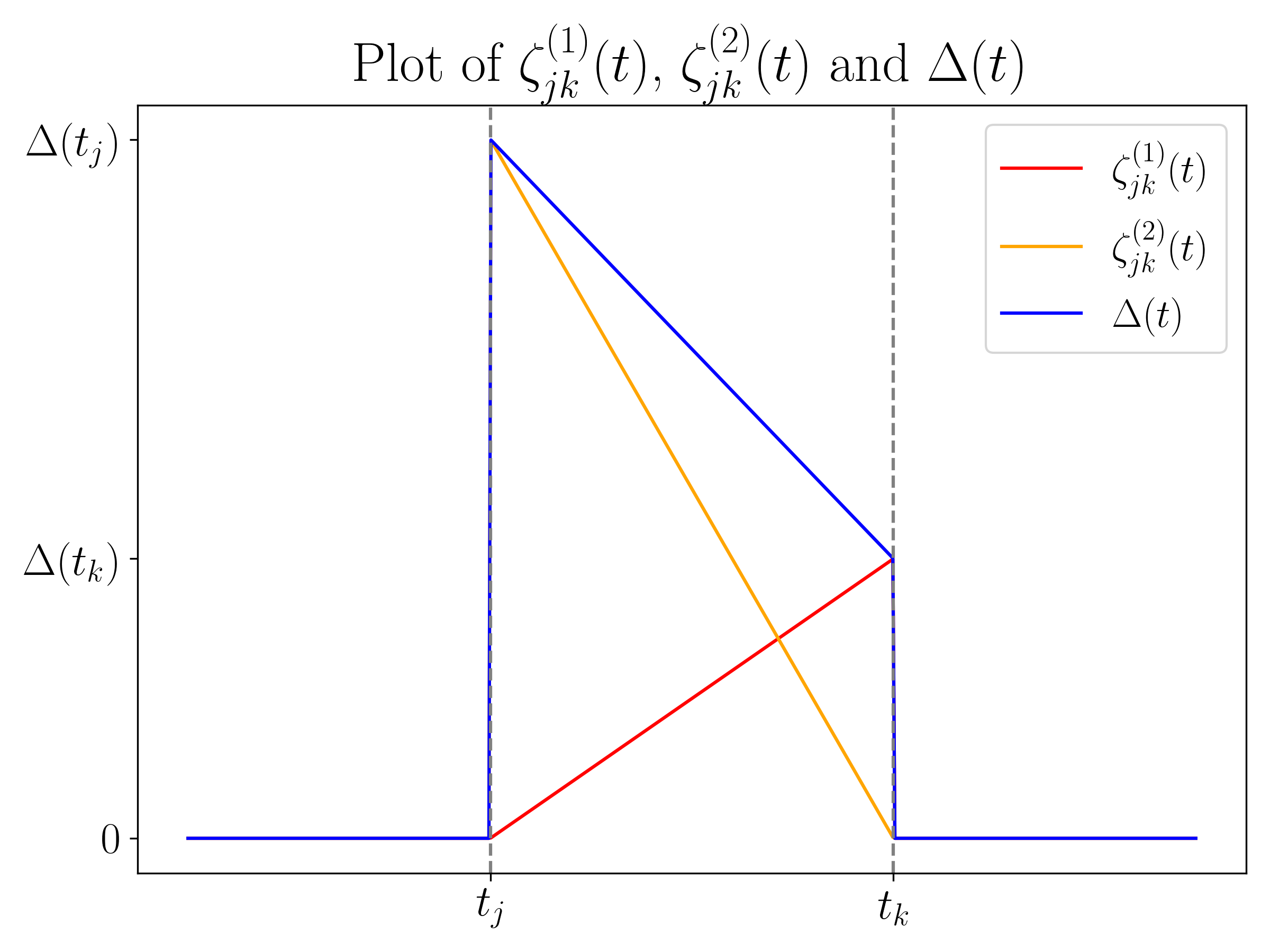
Figure 5:

This shows that there are real coefficients $\lambda_{1},\ldots,\lambda_{4m+4}$ and functions $\zeta_{1},\ldots,\zeta_{4m+4}$ in $\Phi$ such that $\Delta=\sum_{j=1}^{4m+4}\lambda_{j}\zeta_{j}$ on $\left\{U_{1},\ldots,U_{n}\right\}$, and $\lambda_{j}\lambda_{k}\zeta_{j}\zeta_{k}\geq 0$ for all pairs $(j,k)$. Consequently,

$$\frac{\left|\sum_{i=1}^{n}\Delta\left(U_{i}\right)h^{\prime}(\widehat{\phi}_{n}\left(U_{i}\right))E_{i}\right|}{\|\Delta\|_{n}\|o_{h}\|} \leq\frac{\sum_{j=1}^{4m+4}\left|\lambda_{j}\right|\left|\sum_{i=1}^{n}\zeta_{j}\left(U_{i}\right)h^{\prime}(\widehat{\phi}_{n}\left(U_{i}\right))E_{i}\right|}{\left(\sum_{j=1}^{4m+4}\lambda_{j}^{2}\left\|\zeta_{j}\right\|_{n}^{2}\right)^{1/2}\|o_{h}\|}$$

$$\leq\frac{\sum_{j=1}^{4m+4}\left|\lambda_{j}\right|\left\|\zeta_{j}\right\|_{n}}{\left(\sum_{j=1}^{4m+4}\lambda_{j}^{2}\left\|\zeta_{j}\right\|_{n}^{2}\right)^{1/2}}S_{n}$$

$$\leq(4m+4)^{1/2}S_{n}.$$

The last inequality is due to Cauchy-Schwarz inequality

$$\sum_{j=1}^{4m+4}\left|\lambda_{j}\right|\left\|h_{j}\right\|_{n}\times 1=\left(\sum_{j=1}^{4m+4}\lambda_{j}^{2}\left\|h_{j}\right\|_{n}^{2}\right)^{1/2}\left(\sum_{j=1}^{4m+4}1^{2}\right)^{1/2}.$$

Thus by Equation˜34 we have that

$$\mathbb{P}\left\{\sup_{m>0}\sup_{\Delta\in\mathcal{D}_{m}}\frac{\left|\sum_{i=1}^{n}\Delta\left(U_{i}\right)h^{\prime}(\widehat{\phi}_{n}\left(U_{i}\right))E_{i}\right|}{\|\Delta\|_{n}\|o_{h}\|(m+1)^{1/2}}\leq 2\gamma_{o}\sigma(\log n)^{1/2}\right\}\geq 1-2n^{-\frac{4-\gamma_{o}^{2}}{2}},$$

Setting $\gamma=2\gamma_{o}$ we get the result.

F.5 Proof of Lemma˜F.11

We divide the proof in 2 parts. Part A: $(\widehat{\phi}-\phi)\left(t_{o}\right)\geq\xi$ for some $t_{o}\in[a,b]$. Part B: $(\widehat{\phi}-\phi)\left(t_{o}\right)\geq\xi$ for some $t_{o}\in[a+\delta,b-\delta]$.

Part A

Suppose that $(\widehat{\phi}-\phi)\left(t_{o}\right)\geq\xi$ for some $t_{o}\in[a,b]$. Without loss of generality let $t_{o}\leq(a+b)/2$. Define the linear function

$$\widetilde{\phi}(\cdot):=\left\{\begin{array}[]{cc}\phi\left(t_{o}\right)&\text{ if }\alpha=1\\ \phi\left(t_{o}\right)+\phi^{\prime}\left(t_{o}\right)\left(\cdot-t_{o}\right)&\text{ if }\alpha>1,\end{array}\right.$$

where $\sum_{1}^{0}=0$. Define the concave function $\Phi:=\widehat{\phi}-\widetilde{\phi}$. Now, note that by ˜F.4 we have

$$|\widetilde{\phi}-\phi|\leq L|t-t_{o}|^{\alpha}/\alpha,$$ (35)

Now, since by assumption $\sup_{t\in[a,d]}\widehat{\phi}-\phi\geq\xi$ we have

$$\Phi(t_{o})=\widehat{\phi}(t_{o})-\phi(t_{o})\geq\xi.$$ (36)

Now let $0<\delta\leq(b-a)/8$.

• Step 1.A. Since $\Phi$ is concave, it follows that if $\Phi\left(t_{o}+\delta\right)\geq\xi/2$ then, joint with Equation˜36, $\Phi\geq\xi/2$ on $\left[t_{o},t_{o}+\delta\right]$.

• Step 2.A. Now assume $\Phi\left(t_{o}+\delta\right)<\xi/2$. By concavity of $\Phi$ we have

  $$\Phi(t_{o})\underset{\Phi\text{ concave}}{\underbrace{\leq}}\Phi(t_{o}+\delta)-\delta\Phi^{\prime}(t_{o}+\delta)\Rightarrow\Phi^{\prime}(t_{o}+\delta)\leq\delta^{-1}(\underset{<\xi/2}{\underbrace{\Phi(t_{o}+\delta)}}-\underset{\geq\xi}{\underbrace{\Phi(t_{o})}})<-\delta^{-1}\xi/2.$$

  Consequently, for $t\geq t_{o}+3\delta$

  $$\Phi(t) \underset{\Phi\text{ concave}}{\underbrace{\leq}}\underset{<\xi/2}{\underbrace{\Phi(t_{o}+\delta)}}+\underset{\geq 2\delta}{\underbrace{(t-t_{o}-\delta)}}\underset{<-\delta^{-1}\xi/2}{\underbrace{\Phi^{\prime}(t_{o}+\delta)}}$$

  $$<\xi/2-2\delta\delta^{-1}(\xi/2)=-\xi/2.$$

• Step 1.A + 2.A: $\Phi\geq\xi/2$ or $\Phi\leq\xi/2$ on some interval $J\subset\left[t_{o},t_{o}+4\delta\right]$ with length $\delta$. Using this fact and Equation˜35, we have that $t\in J$

  $$\widehat{\phi}-\phi=\Phi+\widetilde{\phi}-\phi\quad\text{ or }\quad\phi-\widehat{\phi}=\phi-\widetilde{\phi}-\Phi,$$

  is greater or equal than

  $$\xi/2-L(t-t_{o})^{\alpha}/\alpha\geq\xi/2-L(4\delta)^{\alpha}/\alpha,$$

  which is greater or equal than $\xi/4$ provided that $\delta\leq\frac{1}{4}\left(\frac{\alpha\xi}{4L}\right)^{1/\alpha}$.

  Part B

  Now suppose that $(\phi-\widehat{\phi})\left(t_{o}\right)\geq\xi$ for some $\xi>0$ and $t_{o}\in[a+\delta,b-\delta]$, where $0<\delta\leq(b-a)/2$. By ˜F.4 and concavity of both $\phi,\widehat{\phi}$ there exist numbers $\gamma,\widehat{\gamma}$ such that

  $$\phi(t)\geq\phi\left(t_{o}\right)+\gamma\left(t-t_{o}\right)-L\left|t-t_{o}\right|^{\alpha}/\alpha,$$

  and

  $$\widehat{\phi}(t)\leq\widehat{\phi}\left(t_{o}\right)+\widehat{\gamma}\left(t-t_{o}\right).$$

  Thus

  $$(\phi-\widehat{\phi})(t)\geq\xi+(\gamma-\widehat{\gamma})\left(t-t_{o}\right)-L\left|t-t_{o}\right|^{\alpha}/\alpha\geq\xi-L\delta^{\alpha},$$

  for all $t$ in the interval $\left[t_{o},t_{o}+\delta\right]$ or $\left[t_{o}-\delta,t_{o}\right]$, depending on the sign of $\gamma-\widehat{\gamma}$. Moreover, $\xi-L\delta^{\alpha}/\alpha\geq\xi/4$, provided that $\delta\leq\left(\frac{3\alpha\xi}{4L}\right)^{1/\alpha}$.

Appendix G Proof of Theorem˜6.6

Let $m=\pi n$ be the asymptotic fraction of points lying in $\mathcal{U}$, where $n$ is the sample size and $\pi=\int_{\mathcal{U}}f_{w}(w)\,dw$. Define the empirical fraction of points in $\mathcal{U}$ as the random quantity

$$\hat{\pi}_{n}=\frac{1}{n}\sum_{t=1}^{n}\mathbf{1}\{w^{(t)}_{i}\in\mathcal{U}\}.$$

By Lemma˜F.9, the event

$$\mathscr{Q}=\left\{\frac{\pi}{\hat{\pi}_{n}}>1-\epsilon_{n}\right\},$$

holds with probability at least $1-1/2(n+2)^{\gamma}$ for some $\gamma>0$, provided that $n$ is sufficiently large and $\epsilon_{n}\to 0$ as $n\to\infty$. Now, we apply Theorem˜F.5, using Remark˜F.6, with the following substitutions:

$$\psi_{0}\leftarrow\psi_{i,\theta},\quad\widehat{\psi}\leftarrow\widehat{\psi}_{i,\theta},\quad\alpha\leftarrow 2,\quad s\leftarrow s_{i},\quad h\leftarrow h_{s_{i}}=d_{s_{i}}^{-1},$$

where $h_{s_{i}}$ is defined in Equation˜3. Intersecting $\mathscr{Q}$ with the high-probability event in Theorem˜F.5 yields the desired result. The only remaining step is to verify that the assumptions of Theorem˜6.6 imply those of Theorem˜F.5.

1. $\psi_{i,\theta}$ is $s_{i}$-concave for some $s_{i}>-1$. According to Proposition˜6.5, this condition is satisfied provided $\psi_{i}$ is $s_{i}$-concave for some $s_{i}>-1$, which holds by Proposition˜4.3 and ˜4.2.

2. ˜F.2 holds uniformly in $\theta\in\mathbb{S}_{N-1}$ because the design points are drawn from an i.i.d. truncated elliptically symmetric distribution with density generator $g>0$ and then $f_{\mathbf{p}}>0$ on any bounded interval, then $\inf_{u\in\mathcal{U}}\inf_{\theta\in\mathbb{S}_{N-1}}f_{\theta^{\top}\mathbf{p}}(u)\geq C$ for some $C=C(\epsilon)>0$.

3. ˜F.3 holds because $y_{i}^{(t)}$ are sub-gaussian (indeed $\psi_{i}$ is bounded and $\varepsilon_{i}^{(t)}$ are sub-gaussian) and $\psi_{i,\theta}$ is bounded uniformly in $\theta\in\mathbb{S}_{N-1}$ by point (2) of Proposition˜6.5.

4. ˜F.4 holds uniformly in $\theta$ because by point (3) of Proposition˜6.5, $\psi_{i,\theta}\in\mathrm{C}^{2}(\mathcal{U})$ which implies $\phi_{i,\theta}=d_{s_{i}}\circ\psi_{i,\theta}\in\mathrm{C}^{2}(\mathcal{U})$ where $d_{s_{i}}\triangleq h^{-1}_{s_{i}}$, defined in Equation˜3.

Appendix H Remark on ˜6.7

˜6.7 informally states that the revenue functions are smooth around the NE. ˜6.7 is satisfied in several scenarios, for example when $-\partial^{2}_{p^{2}}\operatorname{rev}_{i}(p\mid\mathbf{p}_{-i})\geq L$ for all $p\in\mathcal{P}_{i}$ for some $L>0$ independent of $\mathbf{p}_{-i}$. Indeed, in this case, since $\partial_{p}\operatorname{rev}_{i}(\Gamma_{i}(\mathbf{p})\mid\mathbf{p}_{-i})=0$ we have that $\operatorname{rev}_{i}(\Gamma_{i}(\mathbf{p})\mid\mathbf{p}_{-i})-\operatorname{rev}_{i}(p_{i}\mid\mathbf{p}_{-i})\geq L(p_{i}-\Gamma_{i}(\mathbf{p}))^{2}/2$. Now we give some examples where the condition $-\partial^{2}_{p^{2}}\operatorname{rev}_{i}(p\mid\mathbf{p}_{-i})\geq L$ for all $p\in\mathcal{P}_{i}$ for some $L>0$ independent of $\mathbf{p}_{-i}$ is satisfied:

1. Linear demand models (Li et al., 2024). In this case $\operatorname{rev}_{i}(p\mid\mathbf{p}_{-i})=p(\alpha_{i}-\beta_{i}p+\bm{\gamma}_{i}^{\top}\mathbf{p}_{-i})$, and $-\partial^{2}_{p^{2}}\operatorname{rev}_{i}(p\mid\mathbf{p}_{-i})=2\beta_{i}>0$.

2. Concave demand models. If $\psi_{i}$ is such that $\psi_{i}^{\prime}\geq B_{\psi_{i}^{\prime}}$ for some $B_{\psi_{i}^{\prime}}>0$ as in ˜4.1 and is concave, then $\partial_{p}\operatorname{rev}_{i}(p\mid\mathbf{p}_{-i})=\psi_{i}(-\beta_{i}p+\bm{\gamma}_{i}^{\top}\mathbf{p}_{-i})-\beta_{i}p\psi_{i}^{\prime}(-\beta_{i}p+\bm{\gamma}_{i}^{\top}\mathbf{p}_{-i})$, then

   $$-\partial_{p^{2}}^{2}\operatorname{rev}_{i}(p\mid\mathbf{p}_{-i})=2\psi_{i}^{\prime}(-\beta_{i}p+\bm{\gamma}_{i}^{\top}\mathbf{p}_{-i})-\beta_{i}^{2}p\psi_{i}^{\prime\prime}(-\beta_{i}p+\bm{\gamma}_{i}^{\top}\mathbf{p}_{-i})\geq 2\psi_{i}^{\prime}(-\beta_{i}p+\bm{\gamma}_{i}^{\top}\mathbf{p}_{-i})\geq 2B_{\psi_{i}^{\prime}}>0.$$

   Note that, since $\psi_{i}$-concave is equivalent to $1$-concavity, then, by the inclusion property of $s$-concave functions, any (positive and strictly increasing) $s_{i}$-concave $\psi_{i}$ with $s_{i}\geq 1$ satisfies ˜6.7.

3. s-concave demand functions. Suppose that $\psi_{i}$ satisfies ˜4.1 and ˜4.2. Then, by Proposition˜4.3, $\psi_{i}$ is $s_{i}$-concave for some $s_{i}>-1$, and by Proposition˜A.1 this is equivalent to $\psi_{i}^{\prime\prime}\leq(1-s_{i})(\psi_{i}^{\prime})^{2}/\psi_{i}$. This implies that

   $$-\partial_{p^{2}}^{2}\operatorname{rev}_{i}(p\mid\mathbf{p}_{-i}) =2\psi_{i}^{\prime}(-\beta_{i}p+\bm{\gamma}_{i}^{\top}\mathbf{p}_{-i})-\beta_{i}^{2}p\psi_{i}^{\prime\prime}(-\beta_{i}p+\bm{\gamma}_{i}^{\top}\mathbf{p}_{-i})$$

   $$\geq 2\psi_{i}^{\prime}(-\beta_{i}p+\bm{\gamma}_{i}^{\top}\mathbf{p}_{-i})-\beta_{i}^{2}p(1-s_{i})[\psi_{i}^{\prime}(-\beta_{i}p+\bm{\gamma}_{i}^{\top}\mathbf{p}_{-i})]^{2}/\psi_{i}(-\beta_{i}p+\bm{\gamma}_{i}^{\top}\mathbf{p}_{-i})$$

   $$=\psi_{i}^{\prime}(-\beta_{i}p+\bm{\gamma}_{i}^{\top}\mathbf{p}_{-i})\left\{2-\beta_{i}^{2}p(1-s_{i})\psi_{i}^{\prime}(-\beta_{i}p+\bm{\gamma}_{i}^{\top}\mathbf{p}_{-i})/\psi_{i}(-\beta_{i}p+\bm{\gamma}_{i}^{\top}\mathbf{p}_{-i})\right\},$$

   and since $\psi_{i}^{\prime}\geq B_{\psi_{i}^{\prime}}>0$ a sufficient condition is that

   $$2-\beta_{i}^{2}p(1-s_{i})\psi_{i}^{\prime}(-\beta_{i}p+\bm{\gamma}_{i}^{\top}\mathbf{p}_{-i})/\psi_{i}(-\beta_{i}p+\bm{\gamma}_{i}^{\top}\mathbf{p}_{-i})\geq C,$$

   for some constant $C>0$. Note that since $\psi_{i}^{\prime}/\psi_{i}$ is non-negative, for $s_{i}\geq 1$ the condition is trivially satisfied with $C=2$, indeed this condition coincides with the case studied before for concave demand functions. When $s_{i}\in(-1,1)$ the condition becomes

   $$p\frac{d}{dp}\left\{\log\circ\psi_{i}(-\beta_{i}p+\bm{\gamma}_{i}^{\top}\mathbf{p}_{-i})\right\}=-\beta_{i}p\frac{\psi_{i}^{\prime}(-\beta_{i}p+\bm{\gamma}_{i}^{\top}\mathbf{p}_{-i})}{\psi_{i}(-\beta_{i}p+\bm{\gamma}_{i}^{\top}\mathbf{p}_{-i})}\geq-K,$$

   where we set $K=\frac{2-C}{\beta_{i}(1-s_{i})}$. Note that the left-hand side is always negative, then the inequality makes sense if the right-hand side is negative too, i.e. if $0<C\leq 2$, or $K>0$. For example, suppose that $\psi_{i}$ is $0$-concave (i.e. log-concave), that is $\psi_{i}=e^{\phi_{i}}$ for some increasing concave function $\phi_{i}$, where $\phi_{i}$ needs to be increasing in order to guarantee that $\psi_{i}$ is increasing. The condition becomes

   $$\beta_{i}p\phi^{\prime}(-\beta_{i}p+\bm{\gamma}_{i}^{\top}\mathbf{p}_{-i})=p\frac{d}{dp}\log\psi_{i}(-\beta_{i}p+\bm{\gamma}_{i}^{\top}\mathbf{p}_{-i})\leq K,$$

   and it’s easy to see that any $\phi_{i}(x)=ax$ for $a>0$ sufficiently small, indeed the condition becomes $p\leq K/(\beta_{i}a)$ which holds in $\mathcal{P}_{i}$ as long as $K/(\beta_{i}a)\geq\overline{p}_{i}$, or $a\leq K/(\beta_{i}\overline{p}_{i})$. Another example is $\psi_{i}(x)=-1/(x+b)$ for $b$ sufficiently large, indeed the condition becomes $\frac{p}{(-\beta_{i}p+\bm{\gamma_{i}^{\top}\mathbf{p}_{-i}}+b)^{2}}\leq K/\beta_{i}$ or $p\leq K^{*}$ for some $K^{*}(b)>0$, and $b$ mast by such that $K^{*}\geq\overline{p}_{i}$.

4. General condition on derivatives. The condition $-\partial^{2}_{p^{2}}\operatorname{rev}_{i}(p\mid\mathbf{p}_{-i})\geq L$ is satisfied if $|\psi_{i}^{\prime\prime}|\leq B_{\psi_{i}^{\prime\prime}}$ and $2B_{\psi_{i}^{\prime}}>\beta_{i}\bar{p}_{i}B_{\psi_{i}^{\prime\prime}}$, indeed we have

   $$-\partial^{2}_{p^{2}}\operatorname{rev}_{i}(p\mid\mathbf{p}_{-i}) =2\beta_{i}\psi_{i}^{\prime}(-\beta_{i}p+\bm{\gamma}_{i}^{\top}\mathbf{p}_{-i})-\beta_{i}^{2}p\psi_{i}^{\prime\prime}(-\beta_{i}p+\bm{\gamma}_{i}^{\top}\mathbf{p}_{-i})\geq 2\beta_{i}B_{\psi_{i}^{\prime}}-\beta_{i}^{2}\bar{p}_{i}B_{\psi_{i}^{\prime\prime}}>0.$$

References

• Aksoy-Pierson et al. (2013) Margaret Aksoy-Pierson, Gad Allon, and Awi Federgruen. Price competition under mixed multinomial logit demand functions. Management Science, 59(8):1817–1835, 2013.
• Bagnoli & Bergstrom (2006) Mark Bagnoli and Ted Bergstrom. Log-concave probability and its applications. In Rationality and Equilibrium: A Symposium in Honor of Marcel K. Richter, pp.  217–241. Springer, 2006.
• Balabdaoui et al. (2019) Fadoua Balabdaoui, Cécile Durot, and Hanna Jankowski. Least squares estimation in the monotone single index model. Bernoulli, 25(4B):3276–3310, 2019.
• Bertrand (1883) Joseph Bertrand. Review of “theorie mathematique de la richesse sociale” and of “recherches sur les principles mathematiques de la theorie des richesses.”. Journal de savants, 67:499, 1883.
• Besbes et al. (2015) Omar Besbes, Yonatan Gur, and Assaf Zeevi. Non-stationary stochastic optimization. Operations research, 63(5):1227–1244, 2015.
• Birge et al. (2024) John R Birge, Hongfan Chen, N Bora Keskin, and Amy Ward. To interfere or not to interfere: Information revelation and price-setting incentives in a multiagent learning environment. Operations Research, 2024.
• Bobkov & Madiman (2011) Sergey Bobkov and Mokshay Madiman. Concentration of the information in data with log-concave distributions. The Annals of Probability, 39(4):1528–1543, 2011.
• Borzadaran & Borzadaran (2011) GR Mohtashami Borzadaran and HA Mohtashami Borzadaran. Log-concavity property for some well-known distributions. Surveys in Mathematics and its Applications, 6:203–219, 2011.
• Bracale et al. (2025) Daniele Bracale, Moulinath Banerjee, Yuekai Sun, Kevin Stoll, and Salam Turki. Dynamic pricing in the linear valuation model using shape constraints. arXiv preprint arXiv:2502.05776, 2025.
• Brascamp & Lieb (1976) Herm Jan Brascamp and Elliott H Lieb. On extensions of the brunn-minkowski and prékopa-leindler theorems, including inequalities for log concave functions, and with an application to the diffusion equation. Journal of functional analysis, 22(4):366–389, 1976.
• Brillinger (2012) David R Brillinger. A generalized linear model with “gaussian” regressor variables. Selected Works of David Brillinger, pp.  589–606, 2012.
• Chandrasekaran et al. (2009) Karthekeyan Chandrasekaran, Amit Deshpande, and Santosh Vempala. Sampling s-concave functions: The limit of convexity based isoperimetry. In International Workshop on Approximation Algorithms for Combinatorial Optimization, pp.  420–433. Springer, 2009.
• Chen & Chen (2021) Ningyuan Chen and Ying-Ju Chen. Duopoly competition with network effects in discrete choice models. Operations Research, 69(2):545–559, 2021.
• Chen et al. (2019) Xi Chen, Yining Wang, and Yu-Xiang Wang. Nonstationary stochastic optimization under l p, q-variation measures. Operations Research, 67(6):1752–1765, 2019.
• Chen & Farias (2018) Yiwei Chen and Vivek F Farias. Robust dynamic pricing with strategic customers. Mathematics of Operations Research, 43(4):1119–1142, 2018.
• Chmielewski (1981) Margaret Ann Chmielewski. Elliptically symmetric distributions: A review and bibliography. International Statistical Review/Revue Internationale de Statistique, pp.  67–74, 1981.
• Cole & Roughgarden (2014) Richard Cole and Tim Roughgarden. The sample complexity of revenue maximization. In Proceedings of the forty-sixth annual ACM symposium on Theory of computing, pp.  243–252, 2014.
• Cooper et al. (2015) William L Cooper, Tito Homem-de Mello, and Anton J Kleywegt. Learning and pricing with models that do not explicitly incorporate competition. Operations research, 63(1):86–103, 2015.
• Cournot (1838) AA Cournot. Recherches sur les principes mathématiques de la théorie des richesses par augustin cournot (paris, france: chez l. hachette). 1838.
• Cule & Samworth (2010) Madeleine Cule and Richard Samworth. Theoretical properties of the log-concave maximum likelihood estimator of a multidimensional density. Electronic Journal of Statistics, 4:254–270, 2010.
• Delmas et al. (2024) Jean-Pierre Delmas, Mohammed Nabil El Korso, Stefano Fortunati, and Frédéric Pascal. Elliptically symmetric distributions in signal processing and machine learning. Springer, 2024.
• Doss & Wellner (2016) Charles R Doss and Jon A Wellner. Global rates of convergence of the mles of log-concave and s-concave densities. Annals of statistics, 44(3):954, 2016.
• Dümbgen & Rufibach (2009) Lutz Dümbgen and Kaspar Rufibach. Maximum likelihood estimation of a log-concave density and its distribution function: Basic properties and uniform consistency. Bernoulli, 15(1):40–68, 2009.
• Dümbgen et al. (2004) Lutz Dümbgen, Sandra Freitag, and Geurt Jongbloed. Consistency of concave regression with an application to current-status data. Mathematical methods of statistics, 13:69–81, 2004.
• Fan et al. (2024) Jianqing Fan, Yongyi Guo, and Mengxin Yu. Policy optimization using semiparametric models for dynamic pricing. Journal of the American Statistical Association, 119(545):552–564, 2024.
• Federgruen & Hu (2015) Awi Federgruen and Ming Hu. Multi-product price and assortment competition. Operations Research, 63(3):572–584, 2015.
• Gallego & Hu (2014) Guillermo Gallego and Ming Hu. Dynamic pricing of perishable assets under competition. Management Science, 60(5):1241–1259, 2014.
• Gallego & Wang (2014) Guillermo Gallego and Ruxian Wang. Multiproduct price optimization and competition under the nested logit model with product-differentiated price sensitivities. Operations Research, 62(2):450–461, 2014.
• Gallego et al. (2006) Guillermo Gallego, Woonghee Tim Huh, Wanmo Kang, and Robert Phillips. Price competition with the attraction demand model: Existence of unique equilibrium and its stability. Manufacturing & Service Operations Management, 8(4):359–375, 2006.
• Golrezaei et al. (2019) Negin Golrezaei, Adel Javanmard, and Vahab Mirrokni. Dynamic incentive-aware learning: Robust pricing in contextual auctions. Advances in Neural Information Processing Systems, 32, 2019.
• Goyal et al. (2023) Vineet Goyal, Shukai Li, and Sanjay Mehrotra. Learning to price under competition for multinomial logit demand. Available at SSRN 4572453, 2023.
• Groeneboom & Hendrickx (2018) Piet Groeneboom and Kim Hendrickx. Current status linear regression. The Annals of Statistics, 46(4):1415–1444, 2018.
• Han & Wellner (2016) Qiyang Han and Jon A Wellner. Approximation and estimation of s-concave densities via rényi divergences. Annals of statistics, 44(3):1332, 2016.
• Hsieh et al. (2021) Yu-Guan Hsieh, Kimon Antonakopoulos, and Panayotis Mertikopoulos. Adaptive learning in continuous games: Optimal regret bounds and convergence to nash equilibrium. In Conference on Learning Theory, pp.  2388–2422. PMLR, 2021.
• Javanmard (2017) Adel Javanmard. Perishability of data: dynamic pricing under varying-coefficient models. Journal of Machine Learning Research, 18(53):1–31, 2017.
• Javanmard & Nazerzadeh (2019) Adel Javanmard and Hamid Nazerzadeh. Dynamic pricing in high-dimensions. Journal of Machine Learning Research, 20(9):1–49, 2019.
• Kachani et al. (2007) Soulaymane Kachani, Georgia Perakis, and Carine Simon. Modeling the transient nature of dynamic pricing with demand learning in a competitive environment. Network science, nonlinear science and infrastructure systems, pp.  223–267, 2007.
• Keskin & Zeevi (2018) N Bora Keskin and Assaf Zeevi. On incomplete learning and certainty-equivalence control. Operations Research, 66(4):1136–1167, 2018.
• Kirman (1975) Alan P Kirman. Learning by firms about demand conditions. In Adaptive economic models, pp.  137–156. Elsevier, 1975.
• Koenker & Mizera (2010) Roger Koenker and Ivan Mizera. Quasi-concave density estimation. 2010.
• Kuchibhotla et al. (2021) Arun K Kuchibhotla, Rohit K Patra, and Bodhisattva Sen. Semiparametric efficiency in convexity constrained single-index model. Journal of the American Statistical Association, pp.  1–15, 2021.
• Li (1991) Ker-Chau Li. Sliced inverse regression for dimension reduction. Journal of the American Statistical Association, 86(414):316–327, 1991.
• Li et al. (2024) Shukai Li, Cong Shi, and Sanjay Mehrotra. LEGO: Optimal online learning under sequential price competition. Major Revision at Operations Research. Available at SSRN 4803002, 2024.
• Morrow & Skerlos (2011) W Ross Morrow and Steven J Skerlos. Fixed-point approaches to computing bertrand-nash equilibrium prices under mixed-logit demand. Operations research, 59(2):328–345, 2011.
• Mösching & Dümbgen (2020) Alexandre Mösching and Lutz Dümbgen. Monotone least squares and isotonic quantiles. 2020.
• Niculescu & Persson (2006) Constantin Niculescu and Lars-Erik Persson. Convex functions and their applications, volume 23. Springer, 2006.
• Vershynin (2010) Roman Vershynin. Introduction to the non-asymptotic analysis of random matrices. arXiv preprint arXiv:1011.3027, 2010.
• Wan et al. (2022) Yi Wan, Tom Kober, and Martin Densing. Nonlinear inverse demand curves in electricity market modeling. Energy Economics, 107:105809, 2022.
• Wan et al. (2023) Yi Wan, Tom Kober, Tilman Schildhauer, Thomas J Schmidt, Russell McKenna, and Martin Densing. Conditions for profitable operation of p2x energy hubs to meet local demand with energy market access. Advances in Applied Energy, 10:100127, 2023.
• Zhao (2008) Zhibiao Zhao. Parametric and nonparametric models and methods in financial econometrics. 2008.