000–000
0000 xxxx
Leveraging Two-Phase Data for Improved Prediction of Survival Outcomes with Application to Nasopharyngeal Cancer
Abstract
Accurate survival predicting models are essential for improving targeted cancer therapies and clinical care among cancer patients. In this article, we investigate and develop a method to improve predictions of survival in cancer by leveraging two-phase data with expert knowledge and prognostic index. Our work is motivated by two-phase data in nasopharyngeal cancer (NPC), where traditional covariates are readily available for all subjects, but the primary viral factor, Human Papillomavirus (HPV), is substantially missing. To address this challenge, we propose an expert-guided method that incorporates prognostic index based on the observed covariates and clinical importance of key factors. The proposed method makes efficient use of available data, not simply discarding patients with unknown HPV status. We apply the proposed method and evaluate it against other existing approaches through a series of simulation studies and real data example of NPC patients. Under various settings, the proposed method consistently outperforms competing methods in terms of c-index, calibration slope, and integrated Brier score.
By efficiently leveraging two-phase data, the model provides a more accurate and reliable predictive ability of survival models.
keywords:
Nasopharyngeal cancer; Penalized Cox regression; Prognostic index; Survival modeling; Two-phase data1 Introduction
Human papillomavirus (HPV) has been recognized as an important prognostic indicator in head and neck cancer, particularly oropharyngeal cancer (OPC) (Ang et al., 2010). The importance of HPV as a prognostic factor in OPC was found to be significant enough to update the prognostic staging system for OPC to include HPV status, within the latest American Joint Committee on Cancer (AJCC) 8th Edition Cancer Staging System (Lydiatt et al., 2017). However, the prognostic role of HPV in other head and neck sites, such as within the nasopharynx, have not been as well studied. Both the nasopharynx and oropharynx subsites are anatomically contiguous within Waldeyer’s Ring, which is a ring of lymphoid-rich tissue located in the upper aerodigestive tract. Sites within Waldeyer’s ring are postulated to serve as ideal sites for HPV-driven carcinogenesis (Maxwell et al., 2010; Huang et al., 2022). In this context, several studies (Verma et al., 2018; Wotman et al., 2019; Jiang et al., 2016; Wu et al., 2021) have attempted to investigate the prognostic role of HPV in nasopharyngeal carcinoma (NPC). However, a common problem in recent studies on characterizing HPV-induced NPC (Verma et al., 2018; Wotman et al., 2019) is the substantial proportion of unknown HPV status. Wotman et al. (2019) utilized the Surveillance, Epidemiology and End Results (SEER) database in which 70% of the NPC patients had unknown HPV status. Similarly, in the National Cancer Data Base (NCDB) study by Verma et al. (2018), 11,126 patients had unknown HPV status out of a total of 12,389 NPC patients, indicating a nearly 90% rate of missing HPV status.
Although it is possible to analyze the patients with known HPV status only, such an analysis is likely to cause biased estimation and reduce statistical efficiency (Seaman and White, 2013). Alternatively, an imputation method can be applied to handle unknown HPV status. However, while there is no recognized threshold for an acceptable percentage of missing data in imputation approaches, extra caution is warranted given such a high proportion of unknown HPV status in NPC studies. Among different imputation methods, multiple imputation (MI) (Rubin, 2004) has been commonly used in various applications, yet the challenge of consistent variable selection across multiply imputed datasets complicates model interpretation and inference. Several authors (Chen and Wang, 2013; Wood et al., 2008; Wan et al., 2015; Yang et al., 2005) have proposed to tackle the issue of consistent variable selection with MI. Furthermore, a few studies (White and Royston, 2009; Bartlett et al., 2015) have proposed the MI method for survival outcomes; however, there is a lack of methodology and easy-to-use software tools that address consistent variable selection across multiply imputed datasets in survival settings.
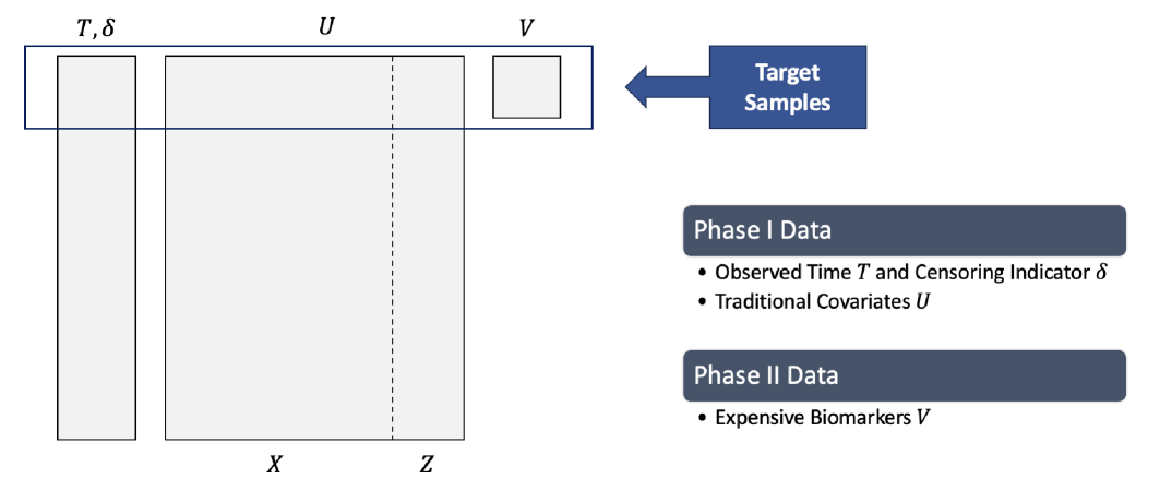
The missing pattern largely coincides with “two-phase” data where a majority of variables are readily available for all subjects with a few covariates of interest being missing. This happens when all patients information on traditional risk factors are gathered, but expensive biomarkers could only be collected on a much smaller cohort. A few studies have considered the use of survival models when data is collected based on a two-phase design (Pal Choudhury et al., 2020; Lumley and Scott, 2013; Breslow and Wellner, 2007). There is, however, scarce literature on efficient use of the two-phase data for survival outcomes with the goal of improving discrimination and calibration.
To address the aforementioned issue, we propose an expert-guided method for the two-phase data. Our goal is to enhance not only discriminatory ability but also calibration of a survival prediction model by efficiently leveraging data, rather than discarding patients with missing data. The proposed method is articulated through a two-stage procedure designed to improve the prediction of survival models. Specifically, we first develop a partially penalized Cox regression model using the full sample and observed variables (e.g., traditional covariates), while allowing covariates identified as crucial based on domain knowledge to be unpenalized. Next, we apply the model obtained from the first stage to the target samples (i.e., a cohort of patients with observed HPV status) to generate predicted risk scores for each individual. These predicted risk scores are referred to as the prognostic index. Finally, we fit the Cox model on the target samples using the prognostic index and key factors (e.g., HPV status) as covariates. This step integrates key expensive biomarkers while adjusting for the prognostic index, which represents a summary measure of an individual’s risk of the event based on the observed covariates.
The prognostic index has been widely adopted for assessing the calibration of validated prognostic models (Mallett et al., 2010; Rahman et al., 2017; Van Houwelingen, 2000). The use of prognostic index also has a close connection to a transfer learning approach which aims to borrow information across different data sources. Recently, Li et al. (2023) adopted transfer learning in the time-to-event outcome framework to transfer knowledge from the source cohort (i.e., large cancer registries) to the target cohort (i.e., a single cancer center). However, such an approach assumes that the same set of variables are available for both cohorts, and thus, is not applicable to our motivating example. In contrast, our proposed method allows the prognostic index to be re-calibrated along with the key factors for further adjustment to the target samples. Re-calibration is a statistical process allows to adapt a risk function to a different population, aiming to eliminate the over- or under-estimation of risk in the importing population (Harrell, 2001; Royston and Altman, 2013). In the extreme scenario where the missingness of HPV status does not depend on any other information (i.e., missing completely at random) and the HPV status itself is not correlated with observed covariates, the estimated slope for the prognostic index will be close to 1, and thus the re-calibrated slope will remain similar. In other cases, including when data is missing at random, the re-calibrated slope will be shifted due to systematic differences by the missing data mechanism (if applicable) and collinearity between the prognostic index and key factors (if present).
The rest of this paper is organized as follows. We briefly present the Cox model and describe the proposed expert-guided method for the two-phase data. We then apply the proposed approach and compare with other existing alternatives through simulation studies and a real data example of NPC patients using the SEER database. In the end, conclusions and discussion are provided.
2 Methods
2.1 Cox regression model and penalization
Assume we observe data from patients, where is the observed time, is the censoring indicator, and is the -dimensional covariates or predictors. In the proportional hazards model, also known as the Cox model (Cox and Oakes, 1984; Cox, 1972), the hazard function is expressed as
| (1) |
where is an unspecified non-negative baseline hazard function and is the parameter vector. The corresponding Cox’s partial likelihood is
where is the index set of death times and is the index set of patients at risk for death at time . The model is assumed to be sparse; that is, a partial set of the contains zero regression coefficients. Then a natural goal is to correctly identify the set of relevant (nonzero) variables.
Penalized methods adopt a shrinkage penalty to combine variable selection with parameter fitting. Denote . The penalized estimates of are obtained by minimizing the following objective function
where is the penalty function which depends on a tuning parameter . There are plenty of choices for the penalty function, including Lasso (Tibshirani, 1996), adaptive Lasso (Zou, 2006), elastic net (Zou and Hastie, 2005), SCAD (Fan and Li, 2001), and Dantzig selector (Candes and Tao, 2007).
2.2 Expert-guided method for two-phase data
For the two-phase data, let and , where denotes the -dimensional traditional variables that are mostly observable and denotes a few expensive -dimensinoal biomarkers which may only be measured on a subsample of patients . Usually, the dimension of is moderate or high, while is low-dimensional. In the example of NPC data, is HPV status which is only observed for a small subset of cohort, and contains baseline covariates, including age, gender, marital status, and so forth. In the following, we introduce an expert-guided method to efficiently handle the two-phase data. The procedure is as follows:
-
I.
In the initial stage, we develop a penalized Cox regression model on the full samples of size using . To reflect domain knowledge in the variable selection process, we decompose into two parts, and , such that , where contains a few key variables that one wishes to retain and contains candidate predictors that are considered for variable selection in a data-driven manner. The hazard function that we consider is
(2) where is the parameter vector. To simultaneously keep in the model and perform variable selection on , we impose a penalty on only. Specifically, we estimate using the partially penalized Cox regression model with adaptive Lasso which minimizes
(3) where is a tuning parameter which controls model complexity and is a vector of weights that are used to adjust a level of penalization on individual covariates. The weights are constructed by for some , where is a root-(/)-consistent estimator. The 5- or 10-fold cross-validation can be used to select an optimal pair of .
-
II.
Next, the model obtained in the initial stage is applied to the target samples of size to generate the prognostic index for each individual. We then fit the Cox model on the target samples using and as covariates. That is, we consider
(4) where the parameter vector is estimated by maximizing the corresponding Cox’s partial likelihood.
The expert-guided method for two-phase data is a two-stage procedure, contrasting with complete case analysis that ignores patients with observed and missing . We consider adaptive Lasso for the penalization in (3) as it ensures that the set of non-zero coefficients is correctly identified with probability converging to one, and the estimated coefficients within this set are asymptotically normal (Zou, 2006). Different procedures have been proposed for constructing adaptive Lasso weights in the literature, including univariable regression (Huang et al., 2008; Sampson et al., 2013) in a low-dimensional setting and a ridge regression (Zou, 2006; Zhang and Lu, 2007) or a preliminary regular Lasso (Benner et al., 2010; Van de Geer et al., 2011; Bühlmann and Van De Geer, 2011) in a high-dimensional setting. However, no consensus has been reached. In the present article, we use perturbed elastic net estimates (Zou and Zhang, 2009) for adaptive Lasso weights. For implementation of the proposed method, we use the R package glmnet (Friedman et al., 2010) in the first stage and survival (Therneau, 2023) in the second stage. Figure 1 below provides an overview of two-phase data and its connection to the proposed expert-guided method. The underlying assumptions regarding the missing mechanism are discussed in Web Appendix A.
Remarks.
-
1.
The prognostic index is a linear combination of selected predictors among weighted by the estimated regression coefficients. It is essentially the log of relative hazard, , which is often utilized for assessing calibration of the predictive models (Mallett et al., 2010; Rahman et al., 2017; Van Houwelingen, 2000). A higher value indicates a worse prognosis when the event is an adverse outcome, such as death or relapse of disease.
-
2.
It is straightforward that the estimated log of relative hazard in (4) becomes equivalent to , since and .
-
3.
In the absence of domain knowledge in the first stage, which precludes the decomposition of into two parts, one may use the model instead of (2). In this case, the penalized Cox regression model is fitted by shrinking all coefficients associated with .
-
4.
All variables are included as covariates in (4), since is usually low-dimensional and contains key variables. However, if a partial set of is known to be clinically irrelevant, one can drop such variables from the model. When there is no prior knowledge about the clinical importance of the entire variables, a simple remedy is to perform a partially penalized Cox regression, similar to the first stage, to retain the prognostic index and assess in a data-driven manner. In the extreme case where is not only one-dimensional but also known to be clinically irrelevant, we suggest merely taking in the second stage.
3 Simulation experiments
In this section, simulation studies are conducted to compare the proposed approach to other existing methods and to evaluate the model performance using various metrics.
3.1 A binary missing covariate
3.1.1 Simulation setup
The survival data are generated from a Weibull distribution with shape parameter 1 and scale parameter 1, following the method of Bender et al. (2005), based on (1). The censoring times are simulated according to an exponential distribution with parameter , which corresponds to a censoring rate of 80%. Traditional covariates are -dimensional standard normal random vector. A binary indicator is randomly generated with success probability conditional on the first variable of , which varies as follows: if ; if ; and if . Data-generating coefficients are set as , along with three different cases: for weak dense (Scenario I); for strong signal (Scenario II); and for moderate concentration (Scenario III). To create two-phase data with being partially available such that , we consider three settings for the missing mechanism: (i) missing completely at random (MCAR); (ii) missing at random (MAR); and (iii) MAR with a mild-to-moderate violation. Details of these settings are provided in Web Appendix B.
For comparison, we analyze the data using our proposed expert-guided (EG) method, complete-case analysis (CCA), naïve imputation (NI) with mode imputation, multiple imputation (MI) following Wood et al. (2008) (hereafter referred to as MI-Wood), and improved MI by Bartlett et al. (2015) using rejection sampling (hereafter referred to as MI-Bartlett). For the MI methods, we consider , where a variable is considered selected if it appears in at least half of the five imputed datasets. The penalty function that we consider across all methods is adaptive Lasso. The 5-fold cross-validation is used to select an optimal for each penalization method. For the proposed EG method, we assume the existence of domain knowledge regarding the clinical importance of and the first two variables in . The predictive model performance is mainly assessed using the c-index, calibration slope, and integrated Brier score (IBS). Variable selection performance on is evaluated by the Matthews correlation coefficient (MCC). A detailed description of each metric is provided in Web Appendix C. The performance measures are evaluated on an independent test set of size . In Web Appendix D, we repeat the analysis by applying domain knowledge to the comparison methods as well.
3.1.2 Simulation results
Model performance metrics are presented with and based on 100 replications. Under the MCAR setting (Table 1), in almost all cases, our proposed EG method outperformed its counterparts in terms of a higher c-index, better calibration, lower IBS, and higher MCC. In contrast, while the NI and the two MI approaches generally performed better than the CCA in terms of c-index, their calibration slopes deviated from the ideal value of 1, signaling inaccurate risk estimates. The MI-Bartlett method outperformed the MI-Wood method in terms of c-index, IBS, and MCC, as missing values were imputed from models which are compatible with the substantive model using rejection sampling. However, the MI-Bartlett method had an issue of overfitting, as indicated by a calibration slope greater than 1 with increased variability. For example, in Scenario I, the MI-Bartlett method produced a calibration slope of 4.72, which deviates substantially from the ideal value of 1. The superiority of the proposed EG method was most apparent in Scenario I, followed by a smaller, yet still noticeable, improvement in Scenario II. In Scenario III, the MI-Bartlett method showed a similar c-index to the EG method, with better IBS and/or MCC. This was expected, as the first two variables of were included in the model based on domain knowledge, making the proposed method less suitable when had no effect. Nonetheless, the EG method consistently provided the best calibration, along with its lower standard deviation, which was nearly one-tenth that of the MI-Bartlett method. Calibration was consistently enhanced using the EG method across various scenarios by integrating the prognostic index and effectively utilizing two-phase data.
| Scenario | Method | c-index | Calibration | IBS | MCC |
|---|---|---|---|---|---|
| slope | |||||
| I | CCA | 0.56 (0.11) | 1.29 (1.64) | 2.25 (0.58) | 0.10 (0.19) |
| NI | 0.61 (0.13) | 1.98 (3.16) | 2.19 (0.62) | 0.25 (0.27) | |
| MI-Wood | 0.59 (0.11) | 2.39 (3.71) | 2.22 (0.56) | 0.20 (0.22) | |
| MI-Bartlett | 0.62 (0.12) | 4.72 (11.3) | 2.21 (0.60) | 0.31 (0.24) | |
| EG | 0.71 (0.11) | 0.94 (0.86) | 2.07 (0.67) | 0.62 (0.11) | |
| II | CCA | 0.66 (0.15) | 1.61 (1.51) | 2.12 (0.80) | 0.34 (0.33) |
| NI | 0.81 (0.09) | 1.91 (1.30) | 1.75 (0.76) | 0.72 (0.19) | |
| MI-Wood | 0.80 (0.09) | 2.30 (2.04) | 1.78 (0.75) | 0.68 (0.15) | |
| MI-Bartlett | 0.81 (0.09) | 2.24 (1.61) | 1.75 (0.78) | 0.74 (0.17) | |
| EG | 0.82 (0.09) | 0.96 (0.54) | 1.74 (0.98) | 0.85 (0.09) | |
| III | CCA | 0.60 (0.12) | 1.56 (1.29) | 2.27 (0.81) | 0.24 (0.32) |
| NI | 0.68 (0.14) | 2.17 (2.15) | 2.07 (0.73) | 0.54 (0.33) | |
| MI-Wood | 0.67 (0.14) | 2.64 (3.86) | 2.05 (0.66) | 0.50 (0.29) | |
| MI-Bartlett | 0.71 (0.14) | 4.14 (7.40) | 1.99 (0.67) | 0.62 (0.28) | |
| EG | 0.72 (0.12) | 0.84 (0.65) | 2.01 (0.78) | 0.56 (0.18) |
Under the setting of MAR (Table 2), the proposed EG method still outperformed the other alternatives in most cases, demonstrating a higher c-index, a calibration slope closer to 1, a smaller IBS, and a higher MCC. Additionally, lower variability in the calibration slope was observed for the EG method. In contrast, the NI and the two MI approaches exhibited poor calibration, with an increased standard deviation observed particularly for both the MI-Wood and MI-Bartlett methods. Substantial variation in the final model with the MI approaches might have been caused by large fluctuations in variable selection results across multiply imputed datasets, in the coefficients of selected variables, or in both. This highlights a major challenge for MI methods when variable selection is involved.
| Scenario | Method | c-index | Calibration | IBS | MCC |
|---|---|---|---|---|---|
| slope | |||||
| I | CCA | 0.57 (0.11) | 2.27 (4.97) | 2.25 (0.77) | 0.09 (0.19) |
| NI | 0.59 (0.13) | 2.06 (3.14) | 2.14 (0.69) | 0.23 (0.26) | |
| MI-Wood | 0.57 (0.11) | 1.93 (3.41) | 2.22 (0.66) | 0.18 (0.23) | |
| MI-Bartlett | 0.60 (0.13) | 5.51 (16.6) | 2.21 (0.73) | 0.29 (0.24) | |
| EG | 0.71 (0.12) | 0.88 (0.75) | 1.94 (0.84) | 0.63 (0.12) | |
| II | CCA | 0.73 (0.15) | 2.42 (4.63) | 1.79 (0.78) | 0.44 (0.28) |
| NI | 0.84 (0.08) | 3.05 (9.57) | 1.41 (0.69) | 0.70 (0.17) | |
| MI-Wood | 0.83 (0.09) | 3.30 (9.57) | 1.46 (0.71) | 0.67 (0.16) | |
| MI-Bartlett | 0.84 (0.08) | 3.20 (9.42) | 1.44 (0.71) | 0.73 (0.15) | |
| EG | 0.85 (0.08) | 1.05 (0.76) | 1.36 (0.64) | 0.85 (0.09) | |
| III | CCA | 0.60 (0.14) | 1.05 (1.69) | 2.12 (0.79) | 0.27 (0.28) |
| NI | 0.69 (0.15) | 2.05 (1.78) | 1.86 (0.78) | 0.52 (0.34) | |
| MI-Wood | 0.68 (0.15) | 2.84 (3.31) | 1.85 (0.70) | 0.49 (0.31) | |
| MI-Bartlett | 0.71 (0.13) | 3.92 (9.29) | 1.84 (0.76) | 0.61 (0.30) | |
| EG | 0.73 (0.13) | 0.81 (0.70) | 1.81 (0.84) | 0.55 (0.18) |
Table 3 presents the performance metrics under a mild-to-moderate violation of the MAR assumption. The c-index for the CCA, NI, and the two MI methods remained similar or had a slight decrease compared to the MAR setting, while the calibration slope increased in nearly all cases, particularly for MI-Bartlett, which deviated further from 1. In contrast, the EG method maintained consistent performance, preserving its superior performance.
| Scenario | Method | c-index | Calibration | IBS | MCC |
|---|---|---|---|---|---|
| slope | |||||
| I | CCA | 0.56 (0.10) | 3.66 (15.4) | 2.28 (0.76) | 0.11 (0.20) |
| NI | 0.58 (0.12) | 1.42 (1.84) | 2.19 (0.66) | 0.23 (0.26) | |
| MI-Wood | 0.58 (0.11) | 2.31 (3.79) | 2.20 (0.65) | 0.19 (0.22) | |
| MI-Bartlett | 0.61 (0.13) | 6.97 (17.5) | 2.22 (0.87) | 0.30 (0.24) | |
| EG | 0.71 (0.12) | 0.91 (0.88) | 1.93 (0.80) | 0.63 (0.12) | |
| II | CCA | 0.72 (0.15) | 2.04 (3.39) | 1.83 (0.78) | 0.40 (0.29) |
| NI | 0.84 (0.09) | 3.58 (13.9) | 1.43 (0.69) | 0.70 (0.17) | |
| MI-Wood | 0.83 (0.09) | 3.14 (9.24) | 1.48 (0.72) | 0.68 (0.13) | |
| MI-Bartlett | 0.83 (0.09) | 3.37 (11.3) | 1.47 (0.71) | 0.73 (0.17) | |
| EG | 0.85 (0.08) | 1.06 (0.77) | 1.40 (0.66) | 0.85 (0.09) | |
| III | CCA | 0.62 (0.14) | 1.65 (2.96) | 2.13 (0.90) | 0.28 (0.28) |
| NI | 0.69 (0.14) | 2.07 (1.83) | 1.87 (0.76) | 0.51 (0.33) | |
| MI-Wood | 0.69 (0.15) | 2.79 (2.87) | 1.87 (0.74) | 0.50 (0.30) | |
| MI-Bartlett | 0.72 (0.14) | 4.24 (10.1) | 1.85 (0.76) | 0.60 (0.27) | |
| EG | 0.73 (0.14) | 0.75 (0.67) | 1.90 (0.95) | 0.56 (0.18) |
3.1.3 Impact of the sample size ratio in two-phase data
We conduct additional simulations to further illustrate the impact of the sample size ratio in two-phase data, i.e., . Due to the characteristics of two-phase data (see Figure 1), is expected to be low, as it typically involves expensive biomarkers. To investigate this, we increase the sample size to , allowing to vary within a reasonable range that ensures both sufficient number of samples and number of events, where (see Web Appendix E). When (Web Table 4), our EG method performed the best. The benefit of our proposed method as compared to the method that discards individuals with missing information (e.g., CCA) was especially evident when the number of the target samples is substantially limited. As increased to (Web Table 5) and (Web Table 6), the difference between our method and the competing methods gradually decreased. However, our method consistently outperformed the alternative approaches in terms of c-index, calibration slope, IBS, and MCC. Additionally, it had a calibration slope very close to 1, regardless of the value of . Thus, the prognostic index contributes to well-calibrated risk predictions, a feature that none of the competing methods achieved.
3.2 A continuous missing covariate
Additional simulations are conducted to evaluate our proposed method in comparison to other methods with a continuous missing covariate. The data-generating distribution and setup resembles Section 3.1 except for , where , and the types of models to be used for imputing variables, including mean imputation for NI and the default imputation methods for MI approaches. Under this simulation design (Web Appendix F), the results remained largely the same as in the binary missing covariate case, demonstrating that our proposed method outperformed its alternatives in terms of a higher c-index, calibration slope closer to 1, lower IBS, and higher MCC in a majority of cases (Web Tables 7–9).
4 Real data application
In this section, we apply our proposed model to the data from Wotman et al. (2019), which comprises patients diagnosed with NPC between 2013–2015 with 3 years of follow-up extracted from the SEER database. Histologically confirmed NPC patients were included using the International Classification of Diseases for Oncology, Third Edition (ICD-O-3), with topography codes for histologic types including 8070, 8071, 8072, 8073, 8020, 8021, and 8082, and site of origin codes including 110, 111, 112, 113, 118, and 119. Patients having malignancies of other head and neck subsites and those with missing follow-up information were excluded from the analysis. Thus, a total of 1,762 NPC patients were included in this analysis with a median follow-up time of 11 months, in which 266 of them died due to NPC. There were 1,245 NPC patients whose HPV status was unknown, leaving only 517 with known HPV status, of whom 180 were tested positive for HPV. Outcome of interest was cause-specific survival in months, which is time from cancer diagnosis to death due to NPC. Patients who died of a cause other than NPC or who were alive by the end of study or lost to follow-up were considered censored at the last date on which they were known to be alive.
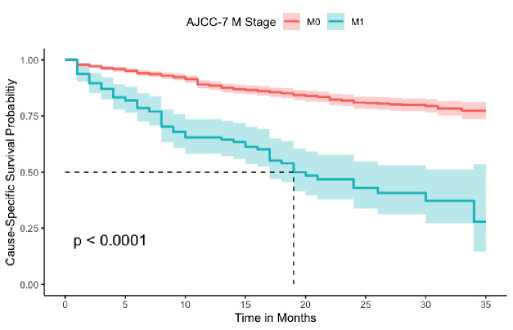
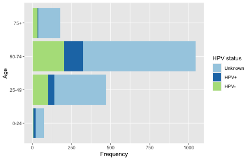
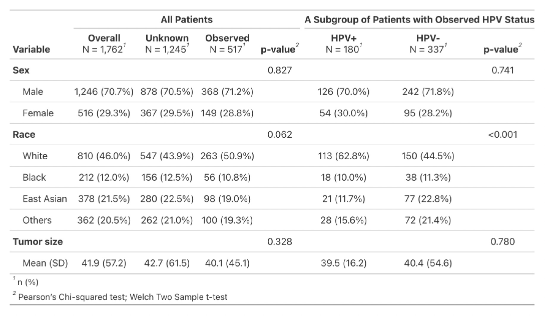
Traditional baseline covariates included gender (male or female), age (25, 25–39, 40–54, 55–69, 70–84, or 85+), marital status (married, single, or other), race (White, Black, East Asians, or other), histology (keratinizing or non-keratinizing), AJCC-7 stage (I/II or III/IV), AJCC-7 T stage (early or advanced), AJCC-7 N stage (0 or 1+), AJCC-7 M stage (M0 or M1), sequence of primary disease (one primary only or other), and tumor size. The HPV status with nearly a 70% missing rate is denoted as in this example. Figure 2 presents clinical and demographic characteristics of the study cohort in terms of age, race, sex, HPV status, AJCC-7 M stage, and tumor size. Figure 2(A) depicts a naïve comparison of cause-specific survival between two groups of AJCC-7 M stage. Figure 2(B) demonstrates that age distribution by HPV status. Figure 2(C) characterizes differences in sex, race, and tumor size using all patients stratified by whether HPV status was observed or not and using a subgroup of patients with observed HPV stratified by whether a patient is HPV+ or HPV–. A full descriptive statistics of the study samples are provided in Web Appendix I.
The proposed method was applied and compared with other methods as in Section 3. The c-index, calibration slope, and IBS were assessed to compare the predictive ability of different models for cause-specific survival in NPC patients. We used 5-fold cross-validation on the target samples of size to create a hold-out test set (20%) for each fold. The remaining 80% of samples, along with samples that had missing HPV status, constituted the training set. We developed a model on each training set and evaluated the performance metrics on each test set. The performance measures were then averaged to obtain an overall estimate of the model performance. For our method, we penalized all variables except for AJCC-7 stage in the first stage based on discussions with domain experts in nasopharyngeal oncology. Additionally, since the existing studies (Verma et al., 2018; Wotman et al., 2019; Jiang et al., 2016; Wu et al., 2021) have linked the prognostic role of HPV to NPC, the HPV status, denoted as , was included in the second stage along with the prognostic index.
The results are summarized in Table 4. Notably, our proposed EG method achieved a higher c-index, a calibration slope closer to 1, and a lower IBS compared to the other methods. The largest difference was observed between the CCA and EG methods, highlighting the disadvantage of analyzing patients with known HPV status only, which incurs a substantial loss of information. The NI the MI methods achieved a c-index of 0.76 and 0.77, respectively. In contrast, the CCA had the lowest c-index of 0.53, while the EG method outperformed all others with the highest c-index of 0.81. The CCA and all three imputation methods did not produce well-calibrated risk estimates, as indicated by the calibration slope deviated from the target value of 1. In particular, the unbiasedness of risk estimation was notable with the proposed EG method which had a calibration slope of 1.07.
| CCA | NI | MI-Wood | MI-Bartlett | EG | |
|---|---|---|---|---|---|
| c-index | 0.53 | 0.76 | 0.77 | 0.77 | 0.81 |
| Calibration slope | 2.67 | 1.14 | 1.20 | 1.20 | 1.07 |
| IBS | 1.30 | 1.23 | 1.21 | 1.21 | 1.14 |
The proposed EG method, which has shown good discrimination and reliable risk estimates, can serve as a key to successful risk stratification and risk-guided clinical decision-making for NPC patients. To demonstrate its utility for risk stratification, we trained our proposed model using the entire dataset and finally applied it to the target samples to divide them into low-, medium-, and high-risk groups. As shown in Web Figure 1, there was a significant difference in cause-specific survival probabilities across these groups () based on the log-rank test. The estimated 2-year cause-specific survival (95% CI) was 93.3% (85.8%, 100.0%) for the low-risk group, 85.1% (79.0%, 91.7%) for the medium-risk group, and 58.7% (46.9%, 73.5%) for the high-risk group. A pairwise log-rank test with the Bonferroni-Holm method of adjustment indicated that there were significant pairwise differences between all three groups. Our study results will help guide therapeutic strategies in clinical practice, including radiation therapy, chemotherapy, or a combination of both, as well as different follow-up care options (e.g., intensive vs. regular monitoring) across various risk groups.
5 Discussion
Accurate survival predictions based on a stable and efficient model enable cancer patients to proactively make plans for their death and achieve goal-concordant care. However, limited efforts have been made towards model updating or leveraging information especially for the two-phase data with survival outcomes. In this paper, we proposed the expert-guided penalized Cox regression model to address several important issues pertinent to the NPC data. Using this method, we efficiently leveraged two-phase data and incorporated domain knowledge into a data-driven variable selection procedure which led to improved prediction of survival outcomes. Additionally, the re-calibration process helped eliminate the over- or under-estimation of risk in the target samples. In contrast, the MI-Bartlett method had overfitting issues, demonstrated by a calibration slope substantially greater than 1, despite having better discriminatory ability compared to the MI-Wood method. While increasing the complexity of the imputation method may improve the model, it also introduces the risk of overfitting when applied to new datasets. It is important to note that when the model fits the training data extremely well with increased complexity, its ability to perform effectively on the independent test data may be compromised.
Through a series of numerical studies and real data application, we have observed that our proposed method achieve a higher c-index, a calibration slope in close proximity of the ideal value of 1, and a lower IBS. To further demonstrate the utility of our approach, we conducted additional simulations with two missing covariates (Web Appendix G). The results largely remained consistent, demonstrating that our proposed method outperformed its alternatives. Additional simulations are warranted to gain a comprehensive understanding of the impact of the missing covariate dimension in two-phase data, by further increasing the number of missing covariates. However, continuously expanding the dimension of becomes less practical in real-world clinical settings, as the resources required to obtain expensive biomarkers may often be limited, not only by the number of individuals that are available for the study, but also by the number of variables that can feasibly be retrieved.
While the prognostic index is re-calibrated along with key factors to adapt to the target samples, a more refined version of the proposed method could allow the prognostic index to differ between the target samples and the remaining ones in the initial step. It is also crucial to recognize that the proposed method can accommodate a variety of penalty functions, although we have primarily focused on adaptive Lasso due to its oracle property. Furthermore, in the absence of domain knowledge about the clinical importance of some variables, the proposed model can still be applied with a slight modification, as illustrated in the Remarks in Section 2.2. The flexibility is one of the major advantages of the proposal.
The proposed method with more reliable and accurate risk estimates can lead to the successful risk-stratified care and clinical support. Especially for cancer patients at the terminal stage, accurate survival estimation will help prevent the overuse of aggressive treatments and reduce unnecessary toxicity. Improved survival estimation is guaranteed only when the proportional hazards assumption holds, which we have assumed throughout the paper. To evaluate the impact of non-proportionality of hazards, additional simulations were conducted (see Web Appendix H). The results showed a reduced c-index and biased risk estimates across all methods, as expected, although the overall impact on our method was relatively small. The variable selection performance was significantly impacted for all methods except our method. Our proposed method experienced only a minimal decrease in MCC, due to the benefit of incorporating domain knowledge and prognostic index. Future research could explore more flexible models that do not rely on the proportional hazards assumption. More complex missing data patterns would further complicate model building and evaluation. We plan to pursue extensions of our proposed work along these lines in future research.
Acknowledgements
We thank the reviewers, the associate editor, and the co-editor for their careful review and thoughtful feedback.
Funding
None declared.
Conflict of interest
None declared.
Data availability
The data that supports the findings in this paper were obtained from the Surveillance, Epidemiology, and End Results (SEER) database of the National Cancer Institute. The SEER data are publicly available at https://seer.cancer.gov. Interested researchers can request access by signing a SEER Research Data Agreement.
Supplementary data
References
- Ang et al. (2010) Ang, K. K., Harris, J., Wheeler, R., Weber, R., Rosenthal, D. I., Nguyen-Tân, P. F., et al. (2010). Human papillomavirus and survival of patients with oropharyngeal cancer. New England Journal of Medicine 363, 24–35.
- Bartlett et al. (2015) Bartlett, J. W., Seaman, S. R., White, I. R., Carpenter, J. R., and Initiative*, A. D. N. (2015). Multiple imputation of covariates by fully conditional specification: accommodating the substantive model. Statistical methods in medical research 24, 462–487.
- Bender et al. (2005) Bender, R., Augustin, T., and Blettner, M. (2005). Generating survival times to simulate cox proportional hazards models. Statistics in medicine 24, 1713–1723.
- Benner et al. (2010) Benner, A., Zucknick, M., Hielscher, T., Ittrich, C., and Mansmann, U. (2010). High-dimensional cox models: the choice of penalty as part of the model building process. Biometrical Journal 52, 50–69.
- Breslow and Wellner (2007) Breslow, N. E. and Wellner, J. A. (2007). Weighted likelihood for semiparametric models and two-phase stratified samples, with application to cox regression. Scandinavian Journal of Statistics 34, 86–102.
- Bühlmann and Van De Geer (2011) Bühlmann, P. and Van De Geer, S. (2011). Statistics for high-dimensional data: methods, theory and applications. Springer Science & Business Media.
- Candes and Tao (2007) Candes, E. and Tao, T. (2007). The dantzig selector: Statistical estimation when p is much larger than n.
- Chen and Wang (2013) Chen, Q. and Wang, S. (2013). Variable selection for multiply-imputed data with application to dioxin exposure study. Statistics in medicine 32, 3646–3659.
- Cox (1972) Cox, D. R. (1972). Regression models and life-tables. Journal of the Royal Statistical Society: Series B (Methodological) 34, 187–202.
- Cox and Oakes (1984) Cox, D. R. and Oakes, D. (1984). Analysis of survival data, volume 21. CRC press.
- Fan and Li (2001) Fan, J. and Li, R. (2001). Variable selection via nonconcave penalized likelihood and its oracle properties. Journal of the American statistical Association 96, 1348–1360.
- Harrell (2001) Harrell, F. E. (2001). Regression modeling strategies: with applications to linear models, logistic regression, and survival analysis, volume 608. Springer.
- Huang et al. (2008) Huang, J., Ma, S., and Zhang, C.-H. (2008). Adaptive lasso for sparse high-dimensional regression models. Statistica Sinica pages 1603–1618.
- Huang et al. (2022) Huang, S. H., Jacinto, J. K., O’Sullivan, B., Su, J., Kim, J., Ringash, J., et al. (2022). Clinical presentation and outcome of human papillomavirus-positive nasopharyngeal carcinoma in a north american cohort. Cancer 128, 2908–2921.
- Jiang et al. (2016) Jiang, W., Chamberlain, P. D., Garden, A. S., Kim, B. Y., Ma, D., Lo, E. J., et al. (2016). Prognostic value of p16 expression in epstein-barr virus–positive nasopharyngeal carcinomas. Head & neck 38, E1459–E1466.
- Li et al. (2023) Li, Z., Shen, Y., and Ning, J. (2023). Accommodating time-varying heterogeneity in risk estimation under the cox model: a transfer learning approach. Journal of the American Statistical Association pages 1–19.
- Lumley and Scott (2013) Lumley, T. and Scott, A. (2013). Partial likelihood ratio tests for the cox model under complex sampling. Statistics in Medicine 32, 110–123.
- Lydiatt et al. (2017) Lydiatt, W. M., Patel, S. G., O’Sullivan, B., Brandwein, M. S., Ridge, J. A., Migliacci, J. C., Loomis, A. M., and Shah, J. P. (2017). Head and neck cancers—major changes in the american joint committee on cancer eighth edition cancer staging manual. CA: a cancer journal for clinicians 67, 122–137.
- Mallett et al. (2010) Mallett, S., Royston, P., Waters, R., Dutton, S., and Altman, D. G. (2010). Reporting performance of prognostic models in cancer: a review. BMC medicine 8, 1–11.
- Maxwell et al. (2010) Maxwell, J. H., Kumar, B., Feng, F. Y., McHugh, J. B., Cordell, K. G., Eisbruch, A., et al. (2010). Hpv-positive/p16-positive/ebv-negative nasopharyngeal carcinoma in white north americans. Head & neck 32, 562–567.
- Pal Choudhury et al. (2020) Pal Choudhury, P., Chaturvedi, A. K., and Chatterjee, N. (2020). Evaluating discrimination of a lung cancer risk prediction model using partial risk-score in a two-phase study. Cancer Epidemiology, Biomarkers & Prevention 29, 1196–1203.
- Rahman et al. (2017) Rahman, M. S., Ambler, G., Choodari-Oskooei, B., and Omar, R. Z. (2017). Review and evaluation of performance measures for survival prediction models in external validation settings. BMC medical research methodology 17, 1–15.
- Royston and Altman (2013) Royston, P. and Altman, D. G. (2013). External validation of a cox prognostic model: principles and methods. BMC medical research methodology 13, 1–15.
- Rubin (2004) Rubin, D. B. (2004). Multiple imputation for nonresponse in surveys, volume 81. John Wiley & Sons.
- Sampson et al. (2013) Sampson, J. N., Chatterjee, N., Carroll, R. J., and Müller, S. (2013). Controlling the local false discovery rate in the adaptive lasso. Biostatistics 14, 653–666.
- Seaman and White (2013) Seaman, S. R. and White, I. R. (2013). Review of inverse probability weighting for dealing with missing data. Statistical methods in medical research 22, 278–295.
- Tibshirani (1996) Tibshirani, R. (1996). Regression shrinkage and selection via the lasso. Journal of the Royal Statistical Society Series B: Statistical Methodology 58, 267–288.
- Van de Geer et al. (2011) Van de Geer, S., Bühlmann, P., and Zhou, S. (2011). The adaptive and the thresholded lasso for potentially misspecified models (and a lower bound for the lasso). Electronic Journal of Statistics 5, 688–749.
- Van Houwelingen (2000) Van Houwelingen, H. C. (2000). Validation, calibration, revision and combination of prognostic survival models. Statistics in medicine 19, 3401–3415.
- Verma et al. (2018) Verma, V., Simone, C. B., and Lin, C. (2018). Human papillomavirus and nasopharyngeal cancer. Head & Neck 40, 696–706.
- Wan et al. (2015) Wan, Y., Datta, S., Conklin, D., and Kong, M. (2015). Variable selection models based on multiple imputation with an application for predicting median effective dose and maximum effect. Journal of statistical computation and simulation 85, 1902–1916.
- White and Royston (2009) White, I. R. and Royston, P. (2009). Imputing missing covariate values for the cox model. Statistics in medicine 28, 1982–1998.
- Wood et al. (2008) Wood, A. M., White, I. R., and Royston, P. (2008). How should variable selection be performed with multiply imputed data? Statistics in medicine 27, 3227–3246.
- Wotman et al. (2019) Wotman, M., Oh, E. J., Ahn, S., Kraus, D., Costantino, P., and Tham, T. (2019). Hpv status in patients with nasopharyngeal carcinoma in the united states: A seer database study. American Journal of Otolaryngology 40, 705–710.
- Wu et al. (2021) Wu, Q., Wang, M., Liu, Y., Wang, X., Li, Y., Hu, X., et al. (2021). HPV positive status is a favorable prognostic factor in non-nasopharyngeal head and neck squamous cell carcinoma patients: a retrospective study from the surveillance, epidemiology, and end results database. Frontiers in oncology 11, 688615.
- Yang et al. (2005) Yang, X., Belin, T. R., and Boscardin, W. J. (2005). Imputation and variable selection in linear regression models with missing covariates. Biometrics 61, 498–506.
- Zhang and Lu (2007) Zhang, H. H. and Lu, W. (2007). Adaptive lasso for cox’s proportional hazards model. Biometrika 94, 691–703.
- Zou (2006) Zou, H. (2006). The adaptive lasso and its oracle properties. Journal of the American statistical association 101, 1418–1429.
- Zou and Hastie (2005) Zou, H. and Hastie, T. (2005). Regularization and variable selection via the elastic net. Journal of the Royal Statistical Society Series B: Statistical Methodology 67, 301–320.
- Zou and Zhang (2009) Zou, H. and Zhang, H. (2009). On the adaptive elastic-net with a diverging number of parameters. Annals of Statistics 37, 1733–1751.