Scalable community detection in massive networks via predictive assignment
Abstract
Massive network datasets are becoming increasingly common in scientific applications. Existing community detection methods encounter significant computational challenges for such massive networks due to two reasons. First, the full network needs to be stored and analyzed on a single server, leading to high memory costs. Second, existing methods typically use matrix factorization or iterative optimization using the full network, resulting in high runtimes. We propose a strategy called predictive assignment to enable computationally efficient community detection while ensuring statistical accuracy. The core idea is to avoid large-scale matrix computations by breaking up the task into a smaller matrix computation plus a large number of vector computations that can be carried out in parallel. Under the proposed method, community detection is carried out on a small subgraph to estimate the relevant model parameters. Next, each remaining node is assigned to a community based on these estimates. We prove that predictive assignment achieves strong consistency under the stochastic blockmodel and its degree-corrected version. We also demonstrate the empirical performance of predictive assignment on simulated networks and two large real-world datasets: DBLP (Digital Bibliography & Library Project), a computer science bibliographical database, and the Twitch Gamers Social Network.
Keywords: Spectral Clustering, Bias-adjusted Spectral Clustering, Stochastic Block Model, Degree Corrected Stochastic Block Model, Computational Efficiency, Scalable Inference
1 Introduction
Community structure is a common feature of networks, where the nodes in a network belong to clusters or communities that exhibit similar behavior [7, 38]. Numerous community detection methods have been developed and studied in the statistics literature, e.g., spectral methods [14, 26, 29], modularity based methods [4, 40], and likelihood based methods [2, 30]. These community detection methods are statistically sound, with rigorous theoretical guarantees, making them valuable tools for network analysis. However, applying these existing methods becomes computationally challenging in many scientific fields where massive networks are becoming increasingly common, e.g., epidemic modeling [33], brain networks [24, 27], online social networks [10, 20], and biomedical text networks [11, 16].
How serious is this problem? To illustrate this, we report a brief computational experiment. Consider an undirected network of nodes with no self-loops, represented by an adjacency matrix , where for . Suppose the network has communities, where is known, with membership vector and membership matrix , where . Under the stochastic block model (SBM) [12], we set , where defines block interactions:
with density parameter and homophily factor . We generated balanced SBMs (each community has nodes) under five scenarios: (i) , (ii) , (iii) , (iv) , (v) . For each scenario, we generated 30 networks and performed community detection using spectral clustering and bias-adjusted spectral clustering [26, 32, 17].
| Spectral Clustering | Bias-adjusted Spectral Clustering | ||||||
|---|---|---|---|---|---|---|---|
| Error (%) | Memory (Mb.) | Runtime (min) | Error (%) | Memory (Mb.) | Runtime (min) | ||
| Memory Overload | |||||||
| Memory Overload | |||||||
| Memory Overload | |||||||
| Memory Overload | |||||||
In Table 1, we report the runtime (in minutes) and memory usage (MB), in addition to the Hamming loss community detection error. We observe that while spectral clustering and its bias-adjusted version are statistically very accurate, with errors close to zero, the computational costs are rather high. Spectral clustering takes 20 minutes for and over 28 minutes for . For bias-adjusted spectral clustering, memory exceeds 8000 MB for (exceeding the 8000 MB RAM of a typical laptop) and 16 GB for , causing a “memory overload” error on the server since it exceeds the 16 GB memory allocation. We would like to point out that the statistical literature on scalable inference tends to focus on runtime as the only measure of computational cost [15, 23, 31]. But in practice, the memory requirement of a statistical method is also a critical component of computational cost. Also note that spectral clustering is one of the fastest community detection algorithms [23, 34], especially with our fast implementation using irlba. Other community detection algorithms, e.g., likelihood-based methods, are likely to fare worse.
In this paper, we introduce predictive assignment, a new technique designed to scale up community detection. The key idea is that if we can have reasonably accurate estimates of the model parameters, we can assign the nodes to communities individually, eliminating the need for clustering. These estimates can be efficiently obtained via community detection on a small subgraph of the network, significantly reducing computational costs compared to community detection on the full network, in the spirit of randomized sketching [35].
Predictive assignment consists of three steps. In Step 1, we select a subsample of nodes from the network. In Step 2, we implement a standard community detection algorithm
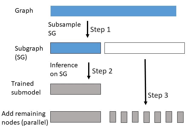
(such as spectral clustering) on the subgraph formed by the subsampled nodes. When the subsample size is small compared to the full network size, this step drastically reduces runtime and memory usage. For example, if the subsample comprises of the nodes, an algorithm would run approximately times faster than on the full network. In Step 3, we assign the remaining nodes to communities by exploiting the mathematical structure of the model. A model assumption (e.g., SBM) provides a structural link between the community memberships of the subgraph nodes (which have already been estimated) and the community memberships of the rest of the nodes (which still need to be estimated). We leverage this structural link to formulate a decision rule that assigns each remaining node to its community using only vector computations. See Figure 1 for a visual illustration.
Predictive assignment is highly versatile as it can accommodate any reasonably accurate community detection method in Step 2 while offering theoretical guarantees of asymptotic accuracy. In this paper, we theoretically analyze predictive assignment under the stochastic blockmodel (defined earlier) as well as the degree corrected blockmodel (DCBM). In Section 3, we prove that under certain mild assumptions, predictive assignment achieves strong consistency in Step 3 (i.e., perfect community assignment with probability tending to 1), even when subgraph community detection in Step 2 is not strongly consistent. Notably, strong consistency holds for any community detection method in Step 2 that meets a specific error bound, making predictive assignment highly robust. Since Step 2 operates on a much smaller subgraph, the overall error rate is primarily influenced by the error from Step 3. Therefore, one could use a fast but relatively less accurate community detection method in Step 2, and still achieve high overall accuracy due to the strong consistency of predictive assignment. In other words, the proposed technique, remarkably, can achieve higher overall accuracy than the underlying community detection method. This phenomenon is further reinforced in our empirical results.
The rest of the paper is organized as follows. In Section 1.1 we describe prior work on scalable community detection. In Section 2, we describe the methodological details of predictive assignment under the SBM and the DCBM, and in Section 3, we study its theoretical properties. In Section 4, we report the computational and statistical performance of predictive assignment in numerical experiments compared to standard community detection as well as existing scalable algorithms. In Section 5, we illustrate the algorithm using two real-world networks: the Digital Bibliography & Library Project (DBLP) database and the Twitch Gamers Social Network. In Section 6 we conclude the paper with a discussion. A supplementary file contains technical proofs of the theoretical results.
1.1 Prior methodologies
In related work, Amini et al., [2] developed a pseudo-likelihood approach to improve the computational efficiency of community detection, and their work was further refined by Wang et al., [34]. Although these methods are highly innovative and have excellent theoretical properties, they rely on a likelihood-based approach that is slower than spectral clustering on the full network, as demonstrated by [23]. Indeed, Wang et al., [34] recommend using spectral clustering on the full network as the initialization step of their algorithm. Since our algorithm is significantly faster than spectral clustering, it is already faster than their initialization step, with subsequent steps only adding to the runtime.
Another approach to scalable community detection is distributed computation. Zhang et al., [39] proposed a distributed community detection algorithm for large networks specifically designed for block models with a grouped community structure. In their model assumption, the group structure overlaps with the community structure such that nodes and communities within the same group have higher link probabilities than those in different groups. While the proposed distributed algorithm in [39] is effective in this setting, their method is limited by this structural assumption. In contrast, our method applies to a broader class of models without requiring such constraints.
Divide-and-conquer strategies have also gained attention as a scalable alternative to direct community detection on large networks [5, 23, 36]. Mukherjee et al., [23] introduced two notable algorithms: PACE (Piecewise Averaged Community Estimation) and GALE (Global Alignment of Local Estimates). The core idea behind both PACE and GALE is a divide and conquer strategy, where subgraphs are sampled from the given network. Community detection is carried out on the subgraphs using some standard community detection method, and the resulting community assignments are aggregated to obtain communities for the full network. Under PACE, this aggregation is carried out in a piecewise manner by considering each pair of nodes and averaging their estimated communities over the subgraphs where both nodes were selected. Under GALE, the aggregation is carried out by using a traversal through the subgraphs. Chakrabarty et al., [5] proposed a divide and conquer strategy using overlapping subgraphs, while Wu et al., [36] developed a distributed computational framework for spectral decomposition under the SBM framework.
Although these divide-and-conquer methods improve scalability, they still require matrix computations for community detection on each subgraph, leading to substantial computational overhead. In contrast, our predictive assignment approach requires matrix computations for only a single subgraph. The remaining nodes are assigned to communities individually through efficient vector-based operations, significantly reducing computational complexity. Morever, predictive assignment also offers stronger theoretical guarantees than the divide-and-conquer methods, as the divide-and-conquer methods can only provide convergence rates of the same order as the underlying community detection algorithm applied to the subgraphs. For predictive assignment, we show in Section 3 that the node assignment in Step 3 can yield strongly consistent community estimates even if the community detection algorithm applied on the single subgraph is weakly consistent. In Section 4.2, we provide a numerical comparison against the methods of Mukherjee et al., [23], highlighting the advantages of our approach in terms of both speed and accuracy.
2 Predictive assignment
We start with some notation. Let denote the set . For any matrix , we use the notation to denote its element and (resp. ) to denote its row (resp. column). For index sets , denotes the sub-matrix of containing the corresponding rows and columns. Let be the diagonal matrix of node degrees, i.e., , and be the diagonal matrix of community sizes from the full network, such that is the number of nodes in the community.
-
1.
Choose via uniform random sampling
-
2.
-
(a)
Carry out community detection on the subgraph .
-
1(b)
Compute the estimates and for . Under SBM,
-
(a)
Assign the remaining nodes to communities (preferably in parallel)
2.1 Steps 1 and 2: subgraph selection and clustering
Let () be the given subsample size. In Step 1, we use some suitable sampling scheme to select a subsample of nodes , where , and select the subgraph spanned by the nodes in . Let be the set of subgraph nodes in the community for . Let be the subgraph version of , such that the diagonal entry of is . We have considered uniform random sampling to select for our theoretical analysis in this paper.
For Step 2, any consistent community detection algorithm under the SBM and DCBM can be used for the subgraph. We recommend the use of fast community detection methods such as spectral clustering and its variants [26, 32]. The chosen community detection method is implemented on the subgraph adjacency matrix to obtain community estimates for all , and, subsequently, the estimates and .
2.2 Step 3: Predictive assignment of the remaining nodes
Next, we use and from Step 2 to estimate a “structural link” parameter, and estimate for .
2.2.1 Closest community approach under SBM
Under the SBM, consider the matrix parameter
| (1) |
and its “plug-in” estimator
| (2) |
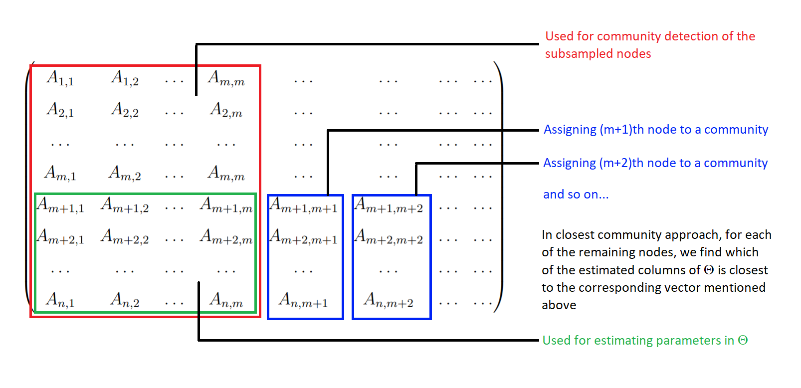
Note that the estimation of via (2) uses community detection results only from the subgraph. Furthermore, this estimator can be computed efficiently since the matrix dimensions in (2) are much smaller than the full adjacency matrix. Consider the node in , and note that its connections to are given by the column vector of the matrix . See Figure 2 for a visual illustration. Denote this column vector as . Then
where is the th column of the identity matrix. Thus, the parameter has two useful properties: it governs the behavior of the non-subgraph nodes, and via (2) it can be estimated using community detection results only from the subgraph. Therefore acts as the “structural link” between the subgraph nodes and the non-subgraph nodes.
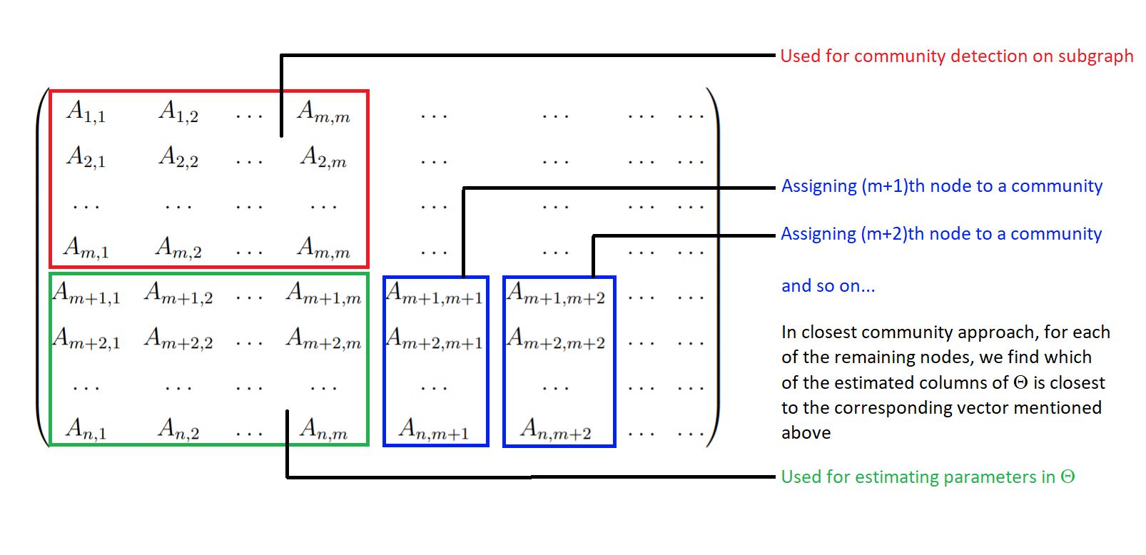
Note that has unique columns, one for each community. Consider the quantity , the distance between and the column of , for . Intuitively, when , represents only the “noise”, whereas when , it represents noise plus bias. Therefore, we expect to have, in a stochastic sense, for any , which implies, heuristically speaking, If we had access to , we could assign the node to its community by simply finding the column of closest to (hence the name closest community). Since we do not observe , we use its estimate from (2) as a proxy. Formally, the assignment rule is
| (3) |
In the top panel of Figure 2, we provide a visual schematic of how the different parts of the adjacency matrix are utilized in this method. From a statistical perspective, the success of this strategy hinges on how accurately we can estimate . In Section 3, we prove that the estimator (2) is indeed sufficiently accurate.
2.2.2 Node popularity approach under DCBM
The DCBM has additional node-specific degree parameters such that . Therefore, for involves the degree parameter , which cannot be estimated from the output of Step 2, which means that the closest community approach no longer works under the DCBM. We propose an alternative approach for predictive assignment based on the concept of node popularity introduced by [30]. The node popularity of the node with respect to the community is defined as the number of edges between the node and the community, i.e., . If is the degree of the th node, then we have
| (4) |
The node-popularity-to-degree ratio within the subgraph is given by
| (5) |
and, the subgraph analogue of the quantity on the right-hand side of (4) is given by
| (6) |
Note that, the ’s defined in (6) are random variables. To estimate the quantities in (6) from the subgraph, observe that can be written as , where is defined as
| (7) |
Thus, under the DCBM, acts as the “structural link” between and . We can estimate from the output of Step 2 as follows:
| (8) |
Then, the community assignment rule is
| (9) |
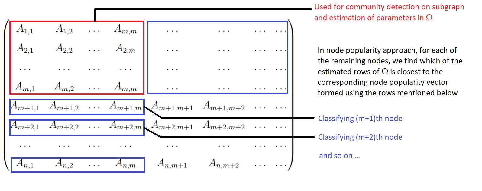
The bottom panel of Figure 2 shows how the different sections of the adjacency matrix are utilized under the node popularity approach. The use of the submatrix in Step 2 is identical to the closest community approach. In Step 3, the blue-bordered vectors are used one by one to assign the remaining nodes to communities. A key difference from the closest community approach is that here we never use the sub-matrix .
We conclude this section with some methodological remarks.
Remark 2.1.
Algorithmic randomness: The random subsampling in Step 1 introduces variability in the estimated subgraph communities, which in turn affects the final community assignments. Theorems 3.1 and 3.2 show that the impact of this algorithmic randomness is negligible as the subgraph retains the necessary properties of the full network with a high probability. One potential strategy to further mitigate the effects of this randomness would be to implement multiple independent runs of the algorithm and then aggregate the results through majority voting. While such an extension would increase computational cost, it may still be more efficient than running full-network community detection while improving robustness. We leave a detailed exploration of this approach for future work.
Remark 2.2.
Out-of-sample extensions of graph embeddings: Predictive assignment is conceptually similar to out-of-sample extensions of graph embeddings [3, 21]. Bengio et al., [3] introduced a framework that interprets these embeddings as eigenfunctions of data-dependent kernels, enabling the extension of learned mappings to new data without recomputing the entire eigendecomposition. Similarly, Levin et al., [21] developed out-of-sample extension methods for incorporating new vertices into existing graph embeddings within the Random Dot Product Graph (RDPG) model, providing theoretical guarantees. A key distinction, however, is that predictive assignment directly estimates community memberships rather than extending a continuous embedding. Our method exploits model-based structural relationships to derive a decision rule for assigning the remaining nodes to communities, whereas out-of-sample graph embedding methods typically extend node positions in an embedding space, which may then be used for clustering or classification.
Remark 2.3.
Semi-supervised community detection: Suppose there exists a set of labeled nodes whose true communities are known, while the remaining nodes in have unknown community labels. The goal of semi-supervised community detection is to estimate the community membership of a new node given its connections to . Jiang and Ke, [13] proposed the Anglemin+ algorithm to address this problem. The algorithm first applies a community detection method to the submatrix to estimate . For a new node , define as , where
Similarly, for each community , define as , where
The new node is assigned to the community which minimizes the angle between and .
To compare this with predictive assignment, note that predictive assignment does not assume the knowledge of a labeled set whose true communities are known. Therefore, we should consider in the context of predictive assignment. However, since the definition of depends on the true communities, Anglemin+ cannot be applied when .
In order to construct a connection between predictive assignment and semi-supervised community detection, one could consider an extension of Anglemin+ that replaces the true community labels in the definitions of and with their estimated versions, i.e.,
and minimizes the angle between the -dimensional vectors and , instead of the -dimensional vectors and . In the notation of predictive assignment, if we put , then becomes (before adjustment) and is the row of in (8). While predictive assignment via node popularity minimizes the Euclidean distance between these vectors (after appropriate scaling), the extended Anglemin+ algorithm would minimize the angle between and . Thus, there are two key distinctions between predictive assignment and Anglemin+. First, predictive assignment relies entirely on estimated communities from the subgraph, whereas Anglemin+ assumes the knowledge of true community labels. Second, the set in predictive assignment is chosen randomly via subsampling, while the labeled set in Anglemin+ is deterministic.
Remark 2.4.
Computational Complexity: Suppose that the complexity of community detection on the full network is given by for some . Extracting the subgraph in Step 1 of predictive assignment requires operations. In Step 2, the complexity of subgraph-based community detection is . The estimation and predictive assignment tasks have a complexity of , which dominates the Step 1 complexity of . Therefore, the complexity of predictive assignment is , compared to for community detection on the full network.
3 Theoretical results
This section describes the theoretical properties of predictive assignment under the SBM and DCBM. We follow the definitions from Sections 1 and 2. In particular, let be the number of nodes and be the number of subsampled nodes. In addition, let and be the size of the th community in the full and subsampled network, respectively, and . Following the standard framework for introducing sparsity into the model [30, 40], we assume that where and is the sparsity parameter such that the expected number of edges in the network is . For the DCBM, following [18], we assume the identifiability constraint for all . We also define , and where is defined in (6). We use , , , , and for absolute constants independent of and ; note that can depend on but not on and . Here, , , , , and can take different values at different instances.
Next, we define error metrics for the different steps of predictive assignment. Assuming optimal label permutation, the average community detection error , and the maximum community-specific error for subgraph community detection in Step 2 are defined as
| (10) |
respectively. The average error in the set of remaining nodes in Step 3 of predictive assignment and the overall error rate (aggregated across Steps 2 and 3) are defined as
| (11) |
respectively. Note that since is much smaller than , the overall error (11) is largely determined by . Next, make the following assumptions:
A1(a). There exists such that
A1(b). Under the DCBM, define . Then, for some constants and
| (12) |
A2. The smallest singular value of is bounded below by a constant .
A3. We have , where for the SBM and for the DCBM.
A4. The sparsity parameter where is a contant and in the case of the SBM.
Here A1(a) is the balanced communities assumption, which states that the community sizes are of the same order of magnitude. A1(b) controls the degree heterogeneity under the DCBM and allows variability of the node degree parameters . Observe that, if the ’s are of the same order of magnitude, A1(b) simply follows from A1(a). Assumption A2 is necessary for identifiability of communities (see, e.g., [18]). Assumption A3 sets lower bounds on the subsample size, which are needed for achieving the required clustering accuracy in the subsample under the SBM and DCBM, respectively. Assumption A4 imposes a lower bound on the sparsity of the sub-network. Under the SBM, we need the subsample size to satisfy . The first condition is satisfied for any reasonably large and small enough , since as . The second condition is only a little stronger than the well-known necessary condition for perfect community detection in an SBM. The full network version of A4, which requires that for some , is a standard assumption in the literature, and is a kind of a necessary condition since leads to impossibility of recovering communities [17, 18]. In A4 we have instead of since this sparsity restriction needs to be imposed on the subgraph. Therefore, A4 seems to be close to the “optimal” fundamental limit under the SBM if is a constant or grows slowly with . Under the DCBM, we impose the additional condition on the degree parameters, given by Noting that by the identifiability constraint for the DCBM, the condition states that there is a trade-off between the sparsity and the degree heterogeneity in the network. If the network is sparse, then the degree heteregeneity in the network should be sufficiently controlled to recover communities.
We are now ready to state our theoretical results. We first need to ensure that a subgraph in Step 1 inherits analogs of the full-sample balance conditions A1(a, b). The next two theorems formalize this and ensure that algorithmic randomness due to subsampling vanishes asymptotically (see Remark 2.1). All technical proofs are in the Appendix.
Theorem 3.1.
Let Assumptions A1(a) and A3 hold. Then,
| (13) |
Theorem 3.1 ensures that, with high probability, the true community proportions of the subgraph adequately represent the true community proportions of the full network.
Theorem 3.2.
Theorem 3.2 ensures that, under the DCBM, the degree parameter-weighted community proportions of the subgraph adequately represent their full-sample counterparts.
Next, we present three “master” theorems that characterize the consistency of parameter estimation and the accuracy of predictive assignment under the SBM and DCBM. These results hold independently of any specific community detection method used in Step 2, thus demonstrating the flexibility of predictive assignment. Suppose that are estimated communities obtained by applying any community detection algorithm to the subgraph such that the maximum community-specific error satisfies
| (16) |
where may depend on and , for some constant , and are constants. In this general framework, the next three theorems provide error bounds for estimating the link parameters and under the SBM and the DCBM. Theorem 3.3 establishes the consistency of parameter estimation under the SBM for both weakly and strongly consistent subgraph community detection. Similarly, Theorem 3.4 establishes parameter estimation consistency under the DCBM for weakly and strongly consistent subgraph community detection.
Theorem 3.3.
(Concentration of ) Suppose that the network is generated from the SBM, and Assumptions A1(a), A2, A3 and A4 hold. If the community detection algorithm on the subgraph satisfies (16), then one has
| (17) |
where , be defined in (1) and (2) respectively. Furthermore, if the community detection algorithm on the subgraph is strong consistent with high probability, that is, , then
| (18) |
Theorem 3.4.
Note that setting to 0 in (19), leads to with probability at least . The sharper error bound in (20) is obtained by more nuanced calculations.
Building on Theorems 3.3 and 3.4, we now present our main result in Theorem 3.5, which establishes that predictive assignment achieves strong consistency for the nodes in under both the SBM and the DCBM.
Theorem 3.5.
Suppose that the network is generated from the SBM or DCBM, and Assumptions A1(a,b), A2, A3 and A4 hold. Assume that
| (21) | |||||
| (22) |
If the constant in Assumption A4 is sufficiently large and for the SBM, or for the DCBM, then for some absolute positive constant , one has
A remarkable implication of Theorem 3.5 is that predictive assignment achieves strong consistency even when subgraph community detection in Step 2 is only weakly consistent, provided that satisfies (21) under the SBM and the (22) under the DCBM. This highlights a key strength of the method: predictive assignment is both computationally efficient and statistically accurate. It allows the use of a fast but less precise community detection algorithm in Step 2, and even if this results in only moderate accuracy for subgraph nodes, Theorem 3.5 guarantees strong consistency for the remaining nodes. Since most nodes in the full network are not part of the subgraph, overall accuracy is determined primarily by the predictive assignment step rather than subgraph community detection. Consequently, because predictive assignment is strongly consistent, the overall accuracy remains high even when subgraph community detection is only moderately accurate.
A natural question at this point is whether there is any advantage in using a strongly consistent community detection method in Step 2. More broadly, does employing a community detection method that achieves better accuracy than (21) or (22) provide any benefits? At first glance, the answer appears to be no, as Theorem 3.5 suggests that additional accuracy is unnecessary. However, the answer is more nuanced and hinges on the lower-bound requirement for . Specifically, the required magnitude of depends on the absolute constants such as , , , , and . When subgraph community detection is strongly consistent, the lower bound requirement on is reduced compared to the weak consistency case, as shown in the proof of Theorem 3.5. A smaller value of would imply that Assumption A4 would be satisfied for smaller values of , meaning a strongly consistent community detection algorithm in Step 2 can help achieve strong consistency on the full network with a lower computational cost. Additionally, increasing allows Assumption A4 to hold for a larger , which leads to faster convergence to perfect clustering. Thus, increasing sharpens the rate at which strong consistency is achieved.
Also note that condition (22) is stricter than condition (21). This implies that, compared to the SBM, more accurate subgraph community detection is needed under the DCBM to achieve strong consistency for predictive assignment.
Finally, we establish in Theorem 3.6 that strong consistency in subgraph community detection is indeed achieved by two well-known algorithms: spectral clustering under the SBM and regularized spectral clustering under the DCBM. While strong consistency for these methods is well established in the literature when applied to the full network [22, 32], this theorem shows that this property extends to the case where the methods are applied to a subgraph spanning randomly subsampled nodes from the full network.
Theorem 3.6.
Suppose that the network is generated from the SBM and Assumptions A1(a), A2, A3 and A4 hold, and spectral clustering is applied to the subgraph; OR, the network is generated from the DCBM and Assumptions A1(a,b), A2, A3 and A4 hold, and regularized spectral clustering is applied to the subgraph. Then, for any , if the constant in Assumption A4 is sufficiently large, there exists an absolute positive constant such that
| (23) |
We conclude this section with the following remark.
Remark 3.1.
Based on the theoretical results, we recommend setting such that , i.e., with . Spectral clustering on the full network achieves strong consistency under the SBM when . In contrast, predictive assignment requires the stronger condition . This highlights the trade-off for scalability when using predictive assignment: achieving strong consistency requires a stricter condition.
4 Simulation studies
We now examine the performance of predictive assignment in synthetic networks generated from the SBM and the DCBM. We compared predictive assignment with community detection on the full network and the two scalable algorithms proposed in [23].
We use the following performance metrics to quantify computational cost and statistical accuracy. For computational performance, the CPU running time and the peak RAM utilization are used to quantify runtime and memory cost, respectively. Note that the peak RAM utilization represents the true memory cost associated with any statistical method and it can be much larger than the size of the input dataset. If the peak RAM value exceeds the computer’s available RAM, it is impossible to execute the code. The proportions of wrongly clustered/assigned nodes , , and , as defined in equations (10) and (11), are used to quantify the statistical performance for the subsampled nodes, the remaining nodes, and the entire set of nodes, respectively. We also report , the percentage of the adjacency matrix used for subgraph clustering in Step 2. Our experiments were performed in R 4.0.2 on a state-of-the-art university high-performance research computing Linux cluster with Intel Xeon processors.
4.1 Predictive assignment vs. full network under the SBM
We first compared the performance of predictive assignment to the benchmark of community detection on the full network. We generated network data from balanced SBMs with block probability matrix such that for ,
where is the overall expected density of the network and is the homophily factor that determines the strength of community structure. We set , , and considered four scenarios: (i) , (ii) , (iii) , and (iv) . We generated random graphs under each case.
We considered two community detection methods for subgraph community detection in Step 2: spectral clustering (SC) and bias-adjusted spectral clustering (BASC). For SC, we compute the orthonormal eigenvectors corresponding to the largest (in absolute value) eigenvalues of the subgraph adjacency matrix , and put them in an matrix. K-means clustering is applied on the matrix rows to estimate the subgraph communities [26, 32]. BASC was proposed by [17], where -means clustering is carried out on the dominant eigenvectors of the “bias-adjusted” matrix instead of . While BASC was proposed for multi-layer networks, we adapt it to single-layer networks in this paper, and extend the method to rectangular (i.e., non-square) submatrices of the adjacency matrix. The key difference between SC and BASC is that they use different portions of the adjacency matrix for subgraph community detection (see Figure 3 in the Appendix for a visual illustration). Note that for SC but for BASC, i.e., BASC uses a much larger proportion of the adjacency matrix. We used for SC, and for BASC. Following Section 2, we used simple random sampling in Step 1 for subgraph selection and the closest community approach in Step 3 for predictive assignment.
| Mem | ||||||
| Bias Adjusted Spectral Clustering | ||||||
| 0.7 | 7.63 | 538.3 | 12.7 1.9 | 9.9 3.8 | 10.0 3.7 | 20.61 |
| 0.75 | 12.93 | 595.0 | 1.0 0.2 | 0.5 0.2 | 0.5 0.1 | 25.32 |
| 0.8 | 21.65 | 725.9 | 0.1 0.0 | 0.1 0.0 | 0.1 0.0 | 37.97 |
| 0.85 | 35.57 | 2038.5 | 0.0 0.0 | 0.0 0.0 | 0.0 0.0 | 70.58 |
| Spectral Clustering | ||||||
| 0.85 | 3.89 | 555.1 | 38.7 3.2 | 6.5 3.5 | 12.9 3.4 | 194.79 |
| 0.9 | 11.49 | 555.1 | 2.9 0.2 | 0.0 0.0 | 1.0 0.1 | 146.84 |
| 0.95 | 33.89 | 555.1 | 0.1 0.0 | 0.4 0.0 | 0.2 0.0 | 150.46 |
| 1 | 100.00 | 555.0 | 0.0 0.0 | 0.0 0.0 | 0.0 0.0 | 233.30 |
| Mem | ||||||
| Bias Adjusted Spectral Clustering | ||||||
| 0.7 | 6.22 | 2175.8 | 2.9 0.6 | 2.0 1.0 | 2.1 1.0 | 46.79 |
| 0.75 | 10.93 | 2212.9 | 0.0 0.0 | 0.0 0.0 | 0.0 0.0 | 61.32 |
| 0.8 | 19.00 | 2556.8 | 0.0 0.0 | 0.0 0.0 | 0.0 0.0 | 108.77 |
| 0.85 | 32.40 | 6634.9 | 0.0 0.0 | 0.0 0.0 | 0.0 0.0 | 231.55 |
| Spectral Clustering | ||||||
| 0.85 | 3.16 | 1907 | 19.7 1.3 | 0.0 0.0 | 3.5 0.2 | 328.76 |
| 0.9 | 10.00 | 1907 | 0.5 0.0 | 0.0 0.0 | 0.2 0.0 | 335.14 |
| 0.95 | 31.62 | 1907 | 0.0 0.0 | 0.0 0.0 | 0.0 0.0 | 437.21 |
| 1 | 100.00 | 1907 | 0 0 | 0.0 0.0 | 0.0 0.0 | 773.96 |
| Mem | ||||||
| Bias Adjusted Spectral Clustering | ||||||
| 0.7 | 5.52 | 4883.9 | 0.0 0.0 | 0.0 0.1 | 0.0 0.1 | 78.68 |
| 0.75 | 9.90 | 4895.8 | 0.0 0.0 | 0.0 0.0 | 0.0 0.0 | 113.83 |
| 0.8 | 17.59 | 5416.4 | 0.2 1.3 | 0.2 1.2 | 0.2 1.2 | 207.30 |
| 0.85 | 30.67 | 13219.3 | 0.0 0.0 | 0.0 0.0 | 0.0 0.0 | 483.47 |
| Spectral Clustering | ||||||
| 0.85 | 2.80 | 4283 | 2.8 0.1 | 0.0 0.0 | 0.5 0.0 | 354.71 |
| 0.9 | 9.22 | 4280 | 0.0 0.0 | 0.0 0.0 | 0.0 0.0 | 364.09 |
| 0.95 | 30.37 | 4284 | 0.0 0.0 | 0.0 0.0 | 0.0 0.0 | 629.26 |
| 1 | 100.00 | 4284 | 0.2 1.4 | 0.0 0.0 | 0.2 1.4 | 1195.43 |
| Mem | ||||||
|---|---|---|---|---|---|---|
| Bias Adjusted Spectral Clustering | ||||||
| 0.7 | 5.07 | 8635.2 | 0.0 0.0 | 0.0 0.0 | 0.0 0.0 | 94.49 |
| 0.75 | 9.23 | 8638.5 | 0.0 0.0 | 0.0 0.0 | 0.0 0.0 | 139.77 |
| 0.8 | 16.65 | 9256.9 | 0.0 0.0 | 0.0 0.0 | 0.0 0.0 | 267.36 |
| Spectral Clustering | ||||||
| 0.85 | 2.57 | 7632 | 0.5 0.0 | 0.0 0.0 | 0.1 0.0 | 346.41 |
| 0.9 | 8.71 | 7632 | 0.0 0.0 | 0.0 0.0 | 0.0 0.0 | 464.65 |
| 0.95 | 29.51 | 7632 | 0.2 1.3 | 0.3 1.4 | 0.2 1.4 | 823.02 |
| 1 | 100.00 | 7632 | 0.2 1.4 | 0.0 0.0 | 0.2 1.4 | 1698.00 |
Overall performance: The results are reported in Tables 2 and 3. Note that represents the baseline setting where spectral clustering is carried out on the full network, as previously reported in Table 1. We observe that predictive assignment is 1.5 times to 18 times faster than SC on the full network. In most cases, predictive assignment also achieves low error rates comparable to the full network. Also note that the choice of affects the memory cost for BASC but not for SC.
Accuracy of predictive assignment: In all cases, we observe that , meaning the predictive assignment in Step 3 is uniformly more (or equally) accurate than subgraph community detection in Step 2. In several cases, such as SC with in Table 2, Case (ii), is much smaller than . Even when using a smaller that results in only a moderately accurate assignment for (e.g., with in Table 2, Case (ii)), predictive assignment can still achieve perfect results ( error) for . This is in line with our theoretical results that predictive assignment is strongly consistent (i.e., even when subgraph community detection is weakly consistent (i.e., ). This highlights the key advantage of our method — predictive assignment is both computationally more efficient and statistically more accurate than direct community detection on the full network. Thus, a fast but moderately accurate community detection method in Step 2 suffices to achieve highly accurate overall results via predictive assignment.
SC or BASC? We next consider the choice of subgraph community detection method in Step 2. BASC was proposed by [17] as a more accurate version of SC when applied to the full network. One would expect this advantage in statistical accuracy to hold for subgraph community detection as well, since BASC uses a much higher proportion of the adjacency matrix () than SC for the same value of and . We observe that this is indeed true; BASC is both faster and more accurate than SC for subgraph community detection. However, BASC is much more expensive than SC in terms of memory. Therefore, we recommend using BASC when it is feasible in terms of storage cost, and using SC otherwise.
4.2 Comparison with existing methods
We now compare the performance of our algorithm with two state-of-the-art algorithms for scalable community detection proposed in [23]: PACE (Piecewise Averaged Community Estimation) and GALE (Global Alignment of Local Estimates). To make the comparison as fair as possible, we used the MATLAB code published by the authors [23] and the SBM model setting from their simulation study. We built a MATLAB implementation of the predictive assignment algorithm specifically for this comparison. Note that elsewhere we used the R implementation of our algorithm, therefore, the runtimes and storage costs reported in this subsection are different from the rest of the paper. We consider the following model settings under the SBM: (i) , average degree , and community proportions (this is the same setup as Table 5 of [23]) ; (ii) , average degree , and balanced communities ; and (iii) , average degree , and balanced communities . Following [23], we used SC (unregularized spectral clustering) and RSC-A (regularized spectral clustering with Amini-type regularization) as the parent algorithms for PACE and GALE and for Step 2 of predictive assignment, with for and for . We used algorithmic hyperparameters recommended by [23] for PACE and GALE, and implemented their code in parallel in MATLAB R2019b with 18 workers.
Table 4 reports community detection error (mean standard error) and average runtime from 50 networks under each model setting. The top panel presents results from SC as the parent algorithm for PACE or GALE and as the community detection algorithm in Step 2 for predictive assignment, and the bottom panel presents results from RSC-A. We observe that predictive assignment is much faster than both PACE and GALE, with runtime savings between 50% and 96%. Predictive assignment also provides higher or similar accuracy as PACE and GALE in most cases.
| Algorithm | s.e. | time | s.e. | time | s.e. | time |
|---|---|---|---|---|---|---|
| SC+PACE | 17.06 0.66 | 4.03 | 0.01 0.01 | 12.29 | 2.37 0.31 | 12.92 |
| SC+GALE | 10.50 0.58 | 5.18 | 1.30 0.29 | 8.51 | 74.68 27.25 | 2.99 |
| SC+Predictive Assignment | 13.55 1.97 | 0.19 | 0.03 0.03 | 0.76 | 1.27 0.20 | 1.00 |
| RSC-A+PACE | 17.09 0.65 | 19.91 | 0.01 0.01 | 24.14 | 2.11 0.26 | 29.32 |
| RSC-A+GALE | 34.02 2.85 | 19.63 | 1.26 0.11 | 20.54 | 25.87 19.48 | 21.05 |
| RSC-A+Predictive Assignment | 27.40 15.52 | 3.13 | 0.02 0.02 | 9.47 | 1.26 0.23 | 8.98 |
4.3 Predictive assignment vs. full network under the DCBM
Similar to Section 4.1, here we compared predictive assignment to community detection on the full network under the DCBM. We generated networks from the DCBM with block probability matrix such that for . As before, is the sparsity parameter and is the homophily factor. The degree parameters were generated from the Beta(1,5) distribution to ensure a positively-skewed degree distribution. The resultant probability matrix was scaled to make the networks 1% dense in expectation. This might make a few ’s greater than 1; while sampling edges, we simply cap such ’s to 1. We considered two settings: (i) , , , and (ii) , , , and generated 30 random graphs under each setting.
To implement predictive assignment, we used simple random sampling (SRS) and random walk sampling (RWS) in Step 1. In RWS, we first sample a node uniformly, then choose one of its neighbors at random to be included in the subgraph [6, 19]. In Step 2, we carried out community detection via regularized spectral clustering (RSC). We compute the dominant eigenvectors of and put them in an matrix, similar to SC. But unlike SC, here we first normalize the rows with respect to the respective Euclidean norms and then apply -means clustering on the normalized rows to estimate the subgraph communities [22]. The node popularity rule (9) was used in Step 3.
We used , and as before represents the full network as baseline. The results in Table 5 are generally in line with the SBM simulation study. We observe that predictive assignment is much faster and requires much less memory than community detection on the full network, with little loss of accuracy. While both SRS and RWS lead to accurate and fast community detection, RWS is generally more accurate and faster but requires more memory. The RWS sampling method leads to denser subgraphs than SRS since higher-degree nodes are more likely to be selected, which requires higher memory but also produces greater accuracy and lower runtime.
| Regularized Spectral clustering | ||||||||||||
| Sampling: SRS | Sampling: RWS | |||||||||||
| Mem | Mem | |||||||||||
| 3 | 0.8 | 1.00 | 877 | 75.6 2.1 | 74.4 2.6 | 74.6 2.6 | 481.4 | 877 | 12.7 0.5 | 16.8 0.2 | 16.4 0.2 | 120.5 |
| 3 | 0.85 | 3.16 | 877 | 32.1 1.6 | 19.1 1.6 | 21.4 1.6 | 318.5 | 877 | 4.7 0.2 | 6.8 0.1 | 6.4 0.1 | 199.0 |
| 3 | 0.9 | 10.00 | 877 | 12.1 0.3 | 5.0 0.1 | 7.2 0.1 | 376.4 | 1288 | 1.4 0.1 | 1.9 0.1 | 1.8 0.0 | 358.0 |
| 3 | 0.95 | 31.62 | 1288 | 3.1 0.1 | 0.8 0.0 | 2.1 0.1 | 661.8 | 1781 | 0.4 0.0 | 0.4 0.0 | 0.4 0.0 | 524.6 |
| 3 | 1 | 100.00 | 2372 | 0.3 0.0 | 0.0 0.0 | 0.3 0.0 | 927.9 | 2372 | 0.3 0.0 | 0.0 0.0 | 0.3 0.0 | 927.9 |
| 5 | 0.8 | 1.00 | 877 | 14.1 0.9 | 7.1 0.6 | 7.8 0.6 | 120.8 | 877 | 1.4 0.1 | 2.1 0.0 | 2.0 0.0 | 102.65 |
| 5 | 0.85 | 3.16 | 877 | 4.3 0.2 | 1.4 0.1 | 1.9 0.1 | 203.5 | 877 | 0.2 0.0 | 0.3 0.0 | 0.3 0.0 | 143.6 |
| 5 | 0.9 | 10.00 | 877 | 0.6 0.1 | 0.1 0.0 | 0.3 0.0 | 289.1 | 1288 | 0.0 0.0 | 0.0 0.0 | 0.0 0.0 | 234.8 |
| 5 | 0.95 | 31.62 | 1288 | 0.0 0.0 | 0.0 0.0 | 0.0 0.0 | 434.7 | 1781 | 0.0 0.0 | 0.0 0.0 | 0.0 0.0 | 414.6 |
| 5 | 1 | 100.00 | 2372 | 0.0 0.0 | 0.0 0.0 | 0.0 0.0 | 696.1 | 2372 | 0.0 0.0 | 0.0 0.0 | 0.0 0.0 | 696.1 |
5 Real-data Applications: DBLP and Twitch networks
The DBLP network consists of computer scientists belonging to communities representing research areas. Two researchers are connected if they published at the same conference [8]. The Twitch user network was curated from the popular streaming service [28]. An edge connects the users if they follow each other. To the extent of our knowledge, this network dataset has not been previously studied in the statistics literature. The dataset has 168k nodes, and the users are labeled with one of the 15 languages based on their primary language of streaming. To avoid working with heavily unbalanced data, we excluded the English-language streamers, who comprised about 122k users. We also removed all users with dead accounts, users with views less than the median views for the entire network, and users with a lifetime less than the median lifetime. Finally, we extracted the largest connected component with nodes and combined the languages into language groups to obtain the communities.
To implement predictive assignment on the DBLP network, we used SC (both adjacency matrix version and Laplacian matrix version) in Step 2 to be consistent with prior SBM-based analysis of this dataset [29]. There is no prior analysis of the Twitch network in the statistics literature, and we used RSC in Step 2 given the extent of degree heterogeneity. Thus, the two networks complement the simulation studies by providing real-world examples under the SBM and DCBM frameworks. For the DBLP network, we used , and, for the Twitch network, we used . 100 random subgraphs were generated for each value of . The results are in Table 6, where represents the full network.
For the DBLP network, SC (adjacency version) on the full network took 3.36 seconds with an error of 10.65. Predictive assignment is approximately two times faster and achieves slightly higher accuracy. SC (Laplacian version) on the DBLP network took 25.90 seconds with an error of 9.96. Predictive assignment is approximately 10 times faster with comparable accuracy. For the Twitch network, RSC on the full network took about 21 seconds with an error of 36.81 for the adjacency version of RSC and an error of 21.14 for the Laplacian version of RSC. Predictive assignment has similar accuracy that varies with , while being 3 to 6 times faster.
These two real-world examples attest that the proposed algorithm achieves accuracy at par with community detection on the full network, but requires runtimes that are only a small fraction of the runtime needed for community detection on the full network.
| DBLP | Twitch | ||||||||
| SC | SC-laplacian | RSC | RSC-laplacian | ||||||
| time | time | time | time | ||||||
| 0.7 | 10.42 1.40 | 1.61 | 10.41 0.29 | 1.68 | 0.8 | 36.28 5.59 | 3.36 | 28.52 3.78 | 3.42 |
| 0.75 | 10.15 0.26 | 1.70 | 10.38 0.26 | 2.01 | 0.85 | 33.61 5.77 | 4.81 | 24.99 2.36 | 4.65 |
| 0.8 | 10.13 0.24 | 1.86 | 10.35 0.20 | 2.39 | 0.9 | 34.74 4.35 | 6.89 | 22.11 1.72 | 6.95 |
| 1 | 10.65 | 3.36 | 9.96 | 22.90 | 1 | 36.81 | 21.25 | 21.14 | 21.22 |
6 Discussion
We propose the predictive assignment algorithm for scalable community detection in massive networks. The theoretical results ascertain the statistical guarantees of the proposed method while the numerical experiments demonstrate that it can substantially reduce computation costs (both runtime and memory) while producing accurate results. In particular, the node assignment in Step 3 has strong consistency, leading to highly accurate overall results even when the subgraph community detection in Step 2 has some errors.
We believe that the key idea of predictive assignment, which is to replace a large-scale matrix computation with a smaller matrix computation plus a large number of vector computations, can be used in other network inference problems beyond community detection, such as model fitting and two-sample testing. This will be an important avenue for future research. Future directions of research also include extending the predictive assignment method to weighted networks, heterogeneous networks, and multilayer networks.
References
- Agterberg et al., [2022] Agterberg, J., Lubberts, Z., and Arroyo, J. (2022). Joint spectral clustering in multilayer degree-corrected stochastic blockmodels. ArXiv: 2212.05053.
- Amini et al., [2013] Amini, A. A., Chen, A., Bickel, P. J., and Levina, E. (2013). Pseudo-likelihood methods for community detection in large sparse networks. Ann. Statist., 41(4):2097–2122.
- Bengio et al., [2003] Bengio, Y., Paiement, J.-f., Vincent, P., Delalleau, O., Roux, N., and Ouimet, M. (2003). Out-of-sample extensions for lle, isomap, mds, eigenmaps, and spectral clustering. Advances in neural information processing systems, 16.
- Bickel and Chen, [2009] Bickel, P. J. and Chen, A. (2009). A nonparametric view of network models and Newman–Girvan and other modularities. Proceedings of the National Academy of Sciences, 106:21068–21073.
- Chakrabarty et al., [2025] Chakrabarty, S., Sengupta, S., and Chen, Y. (2025). Subsampling based community detection for large networks. Statistica Sinica, 35(3):1–42.
- Dasgupta and Sengupta, [2022] Dasgupta, A. and Sengupta, S. (2022). Scalable estimation of epidemic thresholds via node sampling. Sankhya A, 84:321–344.
- Fortunato, [2010] Fortunato, S. (2010). Community detection in graphs. Physics Reports, 486(3):75–174.
- Gao et al., [2009] Gao, J., Liang, F., Fan, W., Sun, Y., and Han, J. (2009). Graph-based consensus maximization among multiple supervised and unsupervised models. Advances in Neural Information Processing Systems, 22:585–593.
- Greene and Wellner, [2017] Greene, E. and Wellner, J. A. (2017). Exponential bounds for the hypergeometric distribution. Bernoulli, 23(3):1911–1950.
- Guo et al., [2022] Guo, Z., Cho, J.-H., Chen, R., Sengupta, S., Hong, M., and Mitra, T. (2022). Safer: Social capital-based friend recommendation to defend against phishing attacks. In Proceedings of the International AAAI Conference on Web and Social Media, volume 16, pages 241–252.
- Gurtcheff and Sharp, [2003] Gurtcheff, S. E. and Sharp, H. T. (2003). Complications associated with global endometrial ablation: the utility of the maude database. Obstetrics & Gynecology, 102(6):1278–1282.
- Holland et al., [1983] Holland, P., Laskey, K., and Leinhardt, S. (1983). Stochastic blockmodels: first steps. Social Networks, 5:109–137.
- Jiang and Ke, [2023] Jiang, Y. and Ke, T. (2023). Semi-supervised community detection via structural similarity metrics. In The Eleventh International Conference on Learning Representations.
- Jin, [2015] Jin, J. (2015). Fast community detection by SCORE. The Annals of Statistics, 43(1):57–89.
- Kleiner et al., [2014] Kleiner, A., Talwalkar, A., Sarkar, P., and Jordan, M. I. (2014). A scalable bootstrap for massive data. Journal of the Royal Statistical Society: Series B (Statistical Methodology), 76(4):795–816.
- Komolafe et al., [2022] Komolafe, T., Fong, A., and Sengupta, S. (2022). Scalable community extraction of text networks for automated grouping in medical databases. Journal of Data Science, 21(3):470–489.
- Lei and Lin, [2023] Lei, J. and Lin, K. Z. (2023). Bias-adjusted spectral clustering in multi-layer stochastic block models. Journal of the American Statistical Association, 118(544):2433–2445.
- Lei and Rinaldo, [2015] Lei, J. and Rinaldo, A. (2015). Consistency of spectral clustering in stochastic block models. The Annals of Statistics, 43(1):215–237.
- Leskovec and Faloutsos, [2006] Leskovec, J. and Faloutsos, C. (2006). Sampling from large graphs. In Proceedings of the 12th ACM SIGKDD international conference on Knowledge discovery and data mining, pages 631–636.
- Leskovec and Mcauley, [2012] Leskovec, J. and Mcauley, J. (2012). Learning to discover social circles in ego networks. Advances in neural information processing systems, 25.
- Levin et al., [2021] Levin, K. D., Roosta, F., Tang, M., Mahoney, M. W., and Priebe, C. E. (2021). Limit theorems for out-of-sample extensions of the adjacency and laplacian spectral embeddings. Journal of Machine Learning Research, 22(194):1–59.
- Lyzinski et al., [2014] Lyzinski, V., Sussman, D. L., Tang, M., Athreya, A., and Priebe, C. E. (2014). Perfect clustering for stochastic blockmodel graphs via adjacency spectral embedding. Electronic journal of statistics, 8(2):2905–2922.
- Mukherjee et al., [2021] Mukherjee, S. S., Sarkar, P., and Bickel, P. J. (2021). Two provably consistent divide-and-conquer clustering algorithms for large networks. Proceedings of the National Academy of Sciences, 118(44):e2100482118.
- Penny et al., [2011] Penny, W. D., Friston, K. J., Ashburner, J. T., Kiebel, S. J., and Nichols, T. E. (2011). Statistical Parametric Mapping: the Analysis of Functional Brain Images. Elsevier.
- Pensky, [2024] Pensky, M. (2024). Davis- kahan theorem in the two-to-infinity norm and its application to perfect clustering. arXiv preprint arXiv:2411.11728.
- Rohe et al., [2011] Rohe, K., Chatterjee, S., and Yu, B. (2011). Spectral clustering and the high-dimensional stochastic blockmodel. The Annals of Statistics, 39(4):1878–1915.
- Roncal et al., [2013] Roncal, W. G., Koterba, Z. H., Mhembere, D., Kleissas, D. M., Vogelstein, J. T., Burns, R., Bowles, A. R., Donavos, D. K., Ryman, S., and Jung, R. E. (2013). MIGRAINE: MRI graph reliability analysis and inference for connectomics. In 2013 IEEE Global Conference on Signal and Information Processing, pages 313–316. IEEE.
- Sarkar and Rózemberczki, [2021] Sarkar, R. and Rózemberczki, B. (2021). Twitch gamers: a dataset for evaluating proximity preserving and structural role-based node embeddings. In Workshop on Graph Learning Benchmarks @TheWebConf 2021, GLB 2021.
- Sengupta and Chen, [2015] Sengupta, S. and Chen, Y. (2015). Spectral clustering in heterogeneous networks. Statistica Sinica, 25:1081–1106.
- Sengupta and Chen, [2018] Sengupta, S. and Chen, Y. (2018). A block model for node popularity in networks with community structure. Journal of the Royal Statistical Society: Series B (Statistical Methodology), 80(2):365–386.
- Sengupta et al., [2016] Sengupta, S., Volgushev, S., and Shao, X. (2016). A subsampled double bootstrap for massive data. Journal of the American Statistical Association, 111(515):1222–1232.
- Sussman et al., [2012] Sussman, D. L., Tang, M., Fishkind, D. E., and Priebe, C. E. (2012). A consistent adjacency spectral embedding for stochastic blockmodel graphs. Journal of the American Statistical Association, 107(499):1119–1128.
- Venkatramanan et al., [2021] Venkatramanan, S., Sadilek, A., Fadikar, A., Barrett, C. L., Biggerstaff, M., Chen, J., Dotiwalla, X., Eastham, P., Gipson, B., Higdon, D., Kucuktunc, O., Lieber, A., Lewis, B. L., Reynolds, Z., Vullikanti, A. K., Wang, L., and Marathe, M. (2021). Forecasting influenza activity using machine-learned mobility map. Nature communications, 12(1):1–12.
- Wang et al., [2023] Wang, J., Zhang, J., Liu, B., Zhu, J., and Guo, J. (2023). Fast network community detection with profile-pseudo likelihood methods. Journal of the American Statistical Association, 118(542):1359–1372.
- Woodruff et al., [2014] Woodruff, D. P. et al. (2014). Sketching as a tool for numerical linear algebra. Foundations and Trends® in Theoretical Computer Science, 10(1–2):1–157.
- Wu et al., [2020] Wu, S., Li, Z., and Zhu, X. (2020). Distributed community detection for large scale networks using stochastic block model. arXiv preprint arXiv:2009.11747.
- Xie, [2024] Xie, F. (2024). Entrywise limit theorems for eigenvectors of signal-plus-noise matrix models with weak signals. Bernoulli, 30:388–418.
- Yanchenko and Sengupta, [2024] Yanchenko, E. and Sengupta, S. (2024). A generalized hypothesis test for community structure in networks. Network Science, page 1–17.
- Zhang et al., [2023] Zhang, S., Song, R., Lu, W., and Zhu, J. (2023). Distributed community detection in large networks. Journal of Machine Learning Research, 24(401):1–28.
- Zhao et al., [2012] Zhao, Y., Levina, E., and Zhu, J. (2012). Consistency of community detection in networks under degree-corrected stochastic block models. The Annals of Statistics, 40:2266–2292.
Supplementary material for “Scalable community detection in massive networks via predictive assignment”: Technical Proofs
A1 Proof of Theorem 3.1
We know that for all . Let and . Corollary 1 of Greene and Wellner, [9] yields that for , , one has
and similarly,
Then, for , since, under Assumption A1(a), , one has
Similarly, one has
Therefore, by Assumption A1(a),
Due to the Assumption A3, one has , which yields
| (A1) |
A2 Proof of Theorem 3.2
From Eq. 2.12 of Greene and Wellner, [9], we have the following result.
Consider a population containing elements, . Let and let be the draw without replacement from this population. Let . Then,
| (A2) |
where and .
Now, using , obtain
since from Assumption A1(b). Therefore,
| (A3) |
due to Assumption A3(b). Hence, (14) is proved.
A3 Proof of Theorem 3.3
For any , one has
| (A5) |
Also, and,
| (A6) |
Note that
| (A7) | ||||
Given , is fixed, and is a function of independent Bernoulli random variables . Therefore, using Bernstein’s inequality, for any , derive
Choosing
yields that with probability at least ,
which implies, with probability at least ,
| (A8) |
invoking (A5) in the final step above.
A4 Proof of Theorem 3.4
Let be the column of the identity matrix. Then,
Derive
| (A13) |
Bounding :
The last step above follows from the definition of .
Bounding : Note that, the -th element of is
This implies,
Hence
| (A15) |
Conclusion: Combining (A13), (A14) and (A15), obtain
| (A16) |
We can construct probability bound for the quantity on the right-hand side above as follows.
First, we have assumed that
Next, from Theorem 3.1, one has
Finally, Theorem 5.2 of [18] yields that under Assumption A4,
Combining together, one has that with probability at least ,
for some positive constant depending on .
Now, we prove the second part of Theorem 3.4. We expand as
| (A17) |
Consider the set in the sample space with . Note that for one has correct community assignments for all nodes in , so that, for any , one has and , which implies that
| (A18) |
Now, concerning the second term on the right-hand side of (A17),
| (A19) |
Using Hoeffding’s inequality, we have
Applying Theorem 3.1 and taking the union bound, we obtain
Combining terms, we conclude
| (A20) |
which completes the proof.
A5 Proof of Theorem 3.5
Case 1: Closest community approach under the SBM
Recall that and are the columns of and respectively. Then, for the closest community approach, can be written as,
Consider a node . Then , and the node is correctly clustered if
| (A21) |
Fix some and . Then,
since for any and . Denoting , obtain
| (A22) |
Bounding : We establish a lower bound for . Let be the diagonal matrix of the true community sizes for the sub-graph . Now,
Now, due to ,
with probability at least , by Assumption A1(a) and Theorem 3.1. Hence, for some positive constant , one has
| (A23) |
Bounding : Let us examine the expression . It is easy to see that given , vectors are constants and the term is only a function of . Then,
The -th summand is bounded above by . Also, note that
Therefore, using Bernstein’s inequality, for any , derive
Choosing
yields that, with probability at least , one has
Note that,
and,
Therefore, with probability at least , one has
since , and is dominated by due to Assumption A4.
Conclusion: Combination of the above inequality and (A22) yields
| (A24) |
Now, it follows from (A23) and Theorem 3.3 that, with probability at least , one has
Here, the right-hand side of the inequality is bounded below by
Therefore, if and the constant in Assumption A4 is sufficiently large, then the quantity above is positive, and one has
which completes the proof.
Case 2: Node popularity approach under the DCBM
For the node popularity approach, can be written as,
The node is correctly clustered if
| (A25) |
Fix some and . Then, by repeated application of the triangle inequality, we obtain
| (A26) |
Bounding :
First, we establish a lower bound for .
Recall that, for any ,
Define diagonal matrices and such that
Let be the column of the identity matrix. Then, can be written as . For , obtain
since by Assumption A2. Therefore,
with probability at least , by Theorem 3.2. Hence, for some positive constant , one has
| (A27) |
Next, we establish upper bounds for and .
Bounding :
Leveraging Theorems 3.2 and 3.4, one has that with probability at least ,
where the final step follows from by Assumption A4.
Now, if , and , then for all sufficiently large , the numerator on the right-hand side above is upper-bounded by for some positive constant . If satisfies , then one has
| (A28) |
Bounding :
Observe that
So, we have
| (A29) |
| (A30) |
Bounding the first term on the right-hand side of (A30): Using Bernstein’s inequality, one has
since . Choosing
yields that, with probability at least ,
Now, for all ,
| (A31) |
with probability at least , using Theorem 3.2. Noting that dominates by Assumption A4, one has
| (A32) |
where is a positive constant depending on .
Bounding the second term on the right-hand side of (A30): Note that is independent of , since . Using Bernstein’s inequality, one has
since . Choosing
one can follow the same argument as before to obtain
| (A34) |
where is a positive constant depending on .
Bounding the third term on the right-hand side of (A30): Recall equations (A5) and (A6) from the proof of Theorem 3.3.
We have assumed that
| (A35) |
which implies
Combining the above inequality with (A31), one has
Note that we did not take an union bound to obtain the above result, as the probability inequality in (A31) considers all and is free from , and the probability inequality in (A35) is free from both and .
A6 Proof of Theorem 3.6
Define , so that , the identity matrix.
Case 1: Spectral clustering under the SBM
Let be
matrices consisting of the leading eigenvectors of and respectively,
and let be the smallest non-zero eigenvalue of .
We first establish a high-probability lower bound on :
using the fact that by Assumption A2.
By Theorem 3.1, obtain that with probability at least ,
| (A38) |
Thereofore, by Corollary 4.1 of Xie, [37], we obtain that under Assumption A4, there exists a orthogonal matrix such that
| (A39) |
with probability at least .
Next, note that if is rank , we can consider for a orthogonal matrix , since , and is a matrix with full rank. So,
Again, applying Theorem 3.1, obtain that with probability at least ,
| (A40) |
Combining (A38), (A39) and (A40), obtain that with probability at least ,
| (A41) |
Note that, the probability statement in Theorem 3.1 concerns with the randomly chosen subsample which is independent of , and hence, independent of .
Now, by Lemma 1 of Pensky, [25], the number of misclassified nodes obtained from estimating the row clusters of by an -approximate solution to K-means problem with input , i.e. the number of misclustered nodes in step 2, is bounded above by
| (A42) |
provided there exists such that
| (A43) |
Here, is the minimum pairwise Euclidean norm separation among the distinct rows of , which doesn’t depend on . Note that by Theorem 3.1 and (A41), one has, with probability at least
| (A44) |
Then, on the same set, due to Assumption A4, one has
Note that, when , inequality (A43) holds if
Hence, if the constant in Assumption A4(a) is large enough, one can choose , so that (A43) holds. Therefore, the events in (A44) imply that
| (A45) |
Now, since and , there will be no such that , if the constant in Assumption A4 is large enough, and perfect clustering is guaranteed, that is, . Finally, we note that by Theorem 3.1 and (A41), the events in (A44) hold with probability at least . This concludes the proof of the first part of the theorem.
Case 2: Regularized spectral clustering under the DCBM
Let be the diagonal matrix containing the degree parameters as its diagonal elements.
Define and ,
and observe that matrix is diagonal and , the identity matrix.
Note that, the -th diagonal element of is
Also define
Let and be matrices, consisting of the leading eigenvectors of and respectively, and be the corresponding diagonal matrices consisting of the leading eigenvalues. Let be the smallest non-zero eigenvalue of . We first establish a high-probability lower bound on :
due to the fact that by Assumption A2.
Let be the orthogonal matrix for which is minimized, and let and be the regularized versions of and respectively, that is,
Note that if is of rank , we can write with a orthogonal matrix , since , and is a matrix of full rank. Choosing yields that , so that, for nodes within the same community, the corresponding rows of matrix will be the same.
Now, by Lemma 1 of Pensky, [25], the number of misclustered nodes in step 2, obtained from estimating the row clusters of by an -approximate solution to K-means problem with input , is bounded above by
| (A47) |
provided there exists such that
| (A48) |
Here is the minimum pairwise Euclidean norm separation between the distinct rows of . Observe that
Defining as the -dimensional unit vector with the -th element equal to 1, derive
| (A49) |
Note that can be expanded as
Therefore,
In the final step above, we used the fact that and by Weyl’s inequality.
Consider the following events:
| (A50) |
The event implies that (A46) holds, that is is bounded away from zero. From Lemma C.3 of [1],
| (A51) |
provided that and are bounded above by a constant. Both of these conditions hold due to Assumption A4 and since is bounded away from zero. Since , one has
So, and together also imply that
| (A52) |
Therefore, the event implies that
| (A53) |
since under Assumption A4.
Since , we have . Noting that since for all , the event implies that
| (A54) |
Plugging (A53) and (A54) into (A49), we obtain
due to Assumption A4.
Note that under the event , (A48) holds if
Also, Since , we have . Therefore, if the constant in Assumption A4 is large enough, we can choose so that (A48) holds. Hence, the event , which constitutes the intersection of all events in in (A44), implies that
| (A55) |
Now, since and , there will not be any such that , if the constant in Assumption A4(b) is large enough. Then, we have perfect clustering, that is, .
Finally, it remains to show that the event occurs with high probability. It follows from Theorems 3.1 and 3.2 that the events and occur with probability at least . By Theorem 5.2 of [18], the event holds with probability at least under Assumption A4. To obtain the lower probability bound for the event , first apply Lemma C.5 of [1] , which states that with probability at least one has
Next, note that , and from Lemma C.6 of [1], with probability at least . Finally, the quantity is bounded above by a constant, as argued earlier. Thus, the event also holds with probability at least . This concludes the proof.
A7 Schematic for predictive assignment under the SBM using BASC for subgraph community detection