Towards Automated Semantic Interpretability in Reinforcement Learning via Vision-Language Models

Abstract

Semantic Interpretability in Reinforcement Learning (RL) enables transparency, accountability, and safer deployment by making the agent’s decisions understandable and verifiable. Achieving this, however, requires a feature space composed of human-understandable concepts, which traditionally rely on human specification and fail to generalize to unseen environments. In this work, we introduce Semantically Interpretable Reinforcement Learning with Vision-Language Models Empowered Automation (SILVA), an automated framework that leverages pre-trained vision-language models (VLM) for semantic feature extraction and interpretable tree-based models for policy optimization. SILVA first queries a VLM to identify relevant semantic features for an unseen environment, then extracts these features from the environment. Finally, it trains an Interpretable Control Tree via RL, mapping the extracted features to actions in a transparent and interpretable manner. To address the computational inefficiency of extracting features directly with VLMs, we develop a feature extraction pipeline that generates a dataset for training a lightweight convolutional network, which is subsequently used during RL. By leveraging VLMs to automate tree-based RL, SILVA removes the reliance on human annotation previously required by interpretable models while also overcoming the inability of VLMs alone to generate valid robot policies, enabling semantically interpretable reinforcement learning without human-in-the-loop.

I Introduction

Reinforcement learning (RL) agents operate in dynamic environments, often developing policies that rely on latent representations not directly interpretable by humans [1]. Ensuring that these learned representations align with human-understandable concepts, a goal often referred to as semantic interpretability, is crucial for ensuring safety and preventing unintended harmful actions. While progress has been made in developing interpretable AI models, achieving semantic interpretability in RL remains particularly challenging  [2].

Semantic interpretability refers to the extent to which a model’s features, decisions, or internal representations can be understood and explained in terms of human-understandable concepts. Achieving this requires two essential components: (1) the inputs to the decision-making model must be intelligible to facilitate downstream interpretation, and (2) the decision-making process must be built with an interpretable model that allows humans to understand and explain its rationale  [3]. In essence, achieving semantic interpretability involves mapping high-dimensional input data to human-understandable features that can serve as a low-dimensional input space for interpretable decision-making models.

To learn an interpretable model on a semantically interpretable feature space, various model classes can be considered, including decision trees and rule-based policies, both of which facilitate explicit reasoning about an agent’s actions. Decision trees have been used to represent policies in a structured, human-readable format [4, 5, 6]. Similarly, rule-based methods, such as logical programs and symbolic reasoning approaches, offer an alternative by encoding policies in a form that can be explicitly followed and verified [7, 8]. Additionally, hierarchical decision-making frameworks have been explored, where high-level policies generate interpretable subgoals while low-level controllers handle execution [9, 10]. However, none of these prior works address high-dimensional image or video inputs; instead, they rely either on human-defined semantic concepts or ground-truth feature vectors provided by the environment.

Existing approaches have attempted to bridge the gap between raw image inputs and interpretable features [11] to facilitate model understanding but fall short in semantic interpretability. Many approaches either produce mathematical or visual representations that do not correspond to human-understandable concepts [12, 13] or rely on predefined feature spaces that aren’t generalize across different environments, using CNNs [14] or ViTs [15] to establish mappings between inputs and semantic features. As a result, human intervention has traditionally played a key role, either by manually defining semantically meaningful feature spaces [16] or by labeling machine-generated features to associate them with semantically meaningful concepts [17].

The emergence of Vision-Language Models (VLMs) has opened new possibilities for overcoming these challenges. These models, known for their capabilities in fine-grained visual understanding, language reasoning, and decision-making  [18, 19, 20], have seen widespread use in various tasks  [19, 21]. In this work, we demonstrate that VLMs can substitute humans in defining and extracting semantic features, serving not merely as a “scarecrow in oz”  [22] or a cost-effective fallback to human labor, but as a scalable and automated solution that matches human performance.

We propose Semantically Interpretable Reinforcement Learning with Vision-Language Models Empowered Automation (SILVA), which is to the best of our knowledge the first automated framework that achieves semantic interpretability in RL and generalizes effectively to unseen environments. By leveraging VLMs to extract features from raw environment inputs and training with Interpretable Control Trees, we manage to provide the rationale behind a RL algorithm in terms of human-understandable concepts. Notably, our framework (i) maintains competitive performance with black-box models while surpassing uninterpretable models built on the same feature space, (ii) supports both image and video inputs, effectively capturing temporal information, (iii) generalizes to unseen environments without human-in-the-loop, and (iv) enables computational efficiency by training a lightweight convolutional network as an alternative to VLM-based feature extraction.

II Related Work

II-A Interpretable Reinforcement Learning

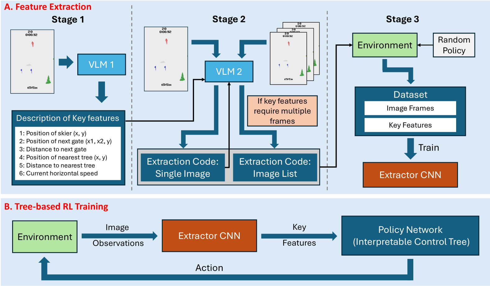
Figure 1: Overview of SILVA, our proposed framework. A. Feature Extraction involves a three-step process where: (1) The VLM identifies key features given domain knowledge and environment observation. (2) The VLM generates code to extract features from a single image frame and assesses whether certain key features require multiple frames. If so, it builds upon the single-frame code to extract these features. (3) Input-output pairs are collected using the extractor code and are used to train an Extractor Convolutional Neural Network (Extractor CNN) as a computationally efficient substitute. B. Tree-based RL Training leverages the Extractor CNN to obtain semantic features from image observations, which are subsequently used as inputs to the policy network (an Interpretable Control Tree) to generate control actions for the RL agent.

Interpretable RL is inherently challenging compared to standard supervised learning, as it involves long-term consequences to actions and latent receptions of data through exploration.  [2] A significant line of research has explored interpretability in RL through generating visual saliency maps using Jacobian-based, perturbation-based, and attribution-based methods [23, 13, 24]. However, these approaches primarily focus on post-hoc explanations and fall out of a stricter definition of Interpretable RL  [3], which requires all components including the input space and the decision-making process to be intelligible. Approaches to achieve intelligible decision-making includes interpretable tree-structures, rule and decision lists, and other rule-based methods [3], among which decision trees are arguably the easiest to verify  [25]. Among state-of-the-art tree methods, Differentiable Decision Trees (DDTs) employ a Decision Tree structure that allows for online learning via stochastic gradient descent [25], while Interpretable Continuous Control Trees (ICCTs) extend this capability to continuous control tasks, ensuring both high performance and interpretability [26]. Similarly, POETREE (Policy Extraction through Decision Trees) [27] introduces dynamically growing probabilistic decision trees that adapt throughout training, allowing the tree complexity to evolve based on the task requirements. Our work addresses the limitation of prior tree-based methods by automating feature definition and extraction, thus enabling generalization to unseen environments.

II-B Feature Extraction for Reinforcement Learning

Common techniques that map high-dimensional inputs into low-dimensional feature spaces for RL includes linear nonparametric methods, such as manifold learning and spectral learning, and nonlinear parametric methods, such as deep learning  [12]. Other work focuses on the extraction of visual features that are not inherently connected with semantic meanings.  [23] employs a self-supervised interpretable network (SSINet) to produce fine-grained attention masks for highlighting task-relevant information.  [13] computed perturbation-based saliency of the image input to deduce regions that had the most effect. However, only a limited number of studies have proposed approaches without human-in-the-loop to construct semantic feature spaces for RL training.  [28] leverages information from Atari instruction manuals to construct the feature space, then uses unsupervised object detection and grounding to acquire the corresponding

objects in the environment. However, they observe that current techniques exhibit a lack of reliability  [28]. Our framework distinguishes from prior work by enabling automatic feature definition and extraction without human-in-the-loop.

II-C VLMs for Reinforcement Learning

VLMs have been applied in various aspects of RL training, including reward design, preference feedback, and representation deriving [29, 30, 20]. One prominent approach involves using VLMs to generate reward functions.  [29] use VLMs as zero-shot reward models to specify tasks via natural language, while  [31] leverages VLMs to produce dense reward functions through code generation. Additionally,  [30, 32] use VLMs to provide preference feedback with which they updated the reward functions for preference-based RL. Another line of work leverages VLMs as feature extractors to obtain valuable information which facilitates training.  [20] extract promptable representations from VLMs and decode output tokens into embeddings, which are used to initialize RL policies. However, those representations are not derived for interpretability purposes and might not often be correct. To the best of our knowledge, our work is the first to utilize VLM for creating a semantic feature space for RL training.

III Methodology

We introduce Semantically Interpretable Reinforcement Learning with Vision-Language Models Empowered Automation (SILVA), a framework designed to automatically learn an interpretable decision-making RL policy from an unseen environment. SILVA leverages the visual comprehension and reasoning capabilities of VLMs automate feature extraction through a three-step pipeline: (1) it employs zero-shot prompting on the environment to identify a set of semantic features that deterministically contribute to the decision-making, (2) it generates feature extraction codes that captures both static and temporal information, and (3) it collects a dataset with VLM-generated extraction codes to train a lightweight convolutional neural network (Extractor CNN) as a computationally efficient substitute. Subsequently, utilizing the Extractor CNN, SILVA performs tree-based RL training with an Interpretable Control Tree, establishing a transparent mapping between the semantic feature space and action outputs to derive a semantically interpretable policy for decision-making.

III-A Feature Extraction

The feature extraction process of SILVA involves a three-step pipeline, as shown in Fig. 1. In Step 1, we query the VLM to generate key features that contribute to the decision in the environment. In Step 2, we query the VLM to generate code that extracts the identified features from the environment, either from a single image or a list of images. In Step 3, we collect a dataset from the environment with the VLM-generated extractor code, with which we train an Extractor CNN that will be used in RL training to enable batch computing and increase program speed. The methodology is formalized below.

Step 1: Querying the VLM for Semantic Features. To extract intelligible features from an unseen environment that could be used to train an effective RL policy, we need to first determine what features are useful to model decision-making. In this step, we provide the VLM with:

• $\mathcal{D}$: Basic domain knowledge about the environment.

• $\mathcal{I}_{0}$: An example image of the environment.

The VLM identifies key semantic features critical for decision-making, represented as two distinct sets:

• $\mathcal{F}_{s}=\{f_{1},f_{2},\dots,f_{p}\}$: Features that can derived from a single image frame.

• $\mathcal{F}_{m}=\{f_{p+1},f_{p+2},\dots,f_{n}\}$: Features requiring multiple frames (e.g., velocity, acceleration, tendency of change). Note that $\mathcal{F}_{m}$ may not be needed in every environment.

The process can be formalized in Eq. 1:

$$\mathcal{F}=\mathcal{F}_{s}\cup\mathcal{F}_{m},\quad\mathcal{F}=\mathcal{M}(\mathcal{D},\mathcal{I}_{0}).$$ (1)

For example, in the Skiing environment, $\mathcal{F}_{s}$ includes features such as the position of skier, the position of next gate, the distance to next gate, the position of nearest tree, and the distance to nearest tree, while $\mathcal{F}_{m}$ includes the current horizontal speed of the skiier. This example is also included in Fig. 1.

Step 2: Querying the VLM for Feature Extraction Code. In this step, we query the VLM to generate feature extraction code, denoted by $\mathcal{G}$, to retrieve the identified set of features $\mathcal{F}$. To mitigate hallucination, we provide visual segmentations for each image, which will be covered in the discussion section. The visual segmentation $\mathcal{S}$ is computed using a segmentation function, represented as $Seg$, such that $\mathcal{S}=\text{Seg}(\mathcal{I})$. The code generation process involves two stages:

Single Image Extraction: For features in $\mathcal{F}$, the VLM generates code $\mathcal{G}_{s}$ to extract as many features as possible from a single image-segmentation pair $(\mathcal{I},\mathcal{S})$. In practice, as demonstrated in our experiments, this approach effectively recovers all features in $\mathcal{F}_{s}$. To enhance the robustness of the generated code, the VLM is provided with multiple example images during this stage to ensure it has been exposed to all possible scenarios. See Algorithm 1.

Multiple Image Extraction: For features in $\mathcal{F}_{m}$, the VLM generates code $\mathcal{G}_{m}$, which extends $\mathcal{G}_{s}$ to process sequential image-segmentation pairs $\{(I_{t-i},S_{t-i}),\dots,(I_{t},S_{t})\}$. One example of such a pair is provided to the VLM during generation. See Algorithm 2.

The final feature extraction code $\mathcal{G}$ is defined in Eq. 2:

$$\mathcal{G}=\begin{cases}\mathcal{G}_{s},&\text{if }\mathcal{F}_{m}=\emptyset;\\ \mathcal{G}_{m}(\mathcal{G}_{s}),&\text{if }\mathcal{F}_{m}\neq\emptyset.\end{cases}$$ (2)

Algorithm 1 Generating Extraction Code: Single Image

1:Input: Feature set $\mathcal{F}$, images $\{\mathcal{I}_{i}\}_{i=1}^{n}$, VLM $\mathcal{M}$

2:Initialize $\mathcal{G}_{s}=null$

3:$examples\leftarrow\emptyset$

4:for each image $\mathcal{I}_{i}$ in $\{\mathcal{I}_{i}\}_{i=1}^{n}$ do

5: $\mathcal{S}_{i}\leftarrow\text{Seg}(\mathcal{I}_{i})$

6: Add $(\mathcal{I}_{i},\mathcal{S}_{i})$ to $examples$

7:end for

8:$\mathcal{G}_{s}\leftarrow\mathcal{M}_{\text{Generate}}(\mathcal{F},examples)$

Algorithm 2 Generating Extraction Code: Image List

1:Input: Feature set $\mathcal{F}$, images $\{\mathcal{I}_{i}\}_{i=1}^{n}$, $\mathcal{G}_{s}$, VLM $\mathcal{M}$

2:Initialize $\mathcal{G}_{m}=null$

3:$examples\leftarrow\emptyset$

4:for each image $\mathcal{I}_{i}$ in $\{\mathcal{I}_{i}\}_{i=1}^{n}$ do

5: $\mathcal{S}_{i}\leftarrow\text{Seg}(\mathcal{I}_{i})$

6: Add $(\mathcal{I}_{i},\mathcal{S}_{i})$ to $examples$

7:end for

8:$\mathcal{F}_{m}\leftarrow{\mathcal{M}_{\text{JudgeMultiFrame}}}(\mathcal{F})$

9:if $\mathcal{F}_{m}\neq\emptyset$ then

10: $\mathcal{G}_{m}\leftarrow\mathcal{M}_{\text{Generate}}(\mathcal{F},examples,\mathcal{G}_{s})$

11:end if

12:Return: $\mathcal{G}_{m}$

Step 3: Dataset Generation and Training an Extractor CNN. In this step, we execute $\mathcal{G}$ on trajectories collected from the environment to generate the feature dataset. For each trajectory, a series of images $\mathcal{T}=\{I_{1},I_{2},\dots,I_{k}\}$ is generated, with corresponding visual segmentations $\mathcal{S}_{t}=\text{Seg}(I_{t})$ for each $t$. The extractor code $\mathcal{G}$ processes each image-segmentation pair $(I_{t},S_{t})$ independently to extract features $\mathbf{v}_{t}=\{v_{1},v_{2},\dots,v_{p}\}$, where $v_{i}\in\mathbb{R}$.

The dataset, consisting of image-feature pairs $\{(\mathcal{I}_{t},\mathbf{v}_{t})\}$, is then used to train an Extractor CNN as a batch-operable and efficient replacement to $\mathcal{G}_{s}$. The trained model predicts semantic features directly from raw images, enabling significantly faster feature extraction during RL training.

If the features require temporal context (i.e., $\mathcal{F}_{m}\neq\emptyset$), $\mathcal{G}_{m}$, consisting of simple mathematical operations on the outputs of $\mathcal{G}_{s}$, is manually adapted to utilize the Extractor CNN in place of $\mathcal{G}_{s}$. For example, in the Skiing environment, $\mathcal{G}_{m}$ retrieves the static features $\mathcal{F}_{s}$ by directly obtaining the values from $\mathcal{G}_{s}$ applied to the last image and acquires the only temporal feature: skiier horizontal speed through subtracting the skiier positions between the first and last image frames. The manual adaptation preserves the exact same logic while ensuring that the subtraction operation is properly batched, significantly accelerating the training process by several orders of magnitude. Without this adaptation, training would be prohibitively time-consuming.

Discussion. Recognizing that hallucination is a well-documented challenge in generative VLM models [33], we provide segmentation along with raw images in Step 2 and 3, using a pre-defined segmentation function $Seg$ that detects objects and their positions in an image by contour and color analysis (details provided in Appendix VII-B). This strategy aligns with common practices in the field [34, 35]. By incorporating segmentation, we mitigate the risk of hallucination and ensure that the generated features and codes are grounded in accurate visual data.

TABLE I: Prompting statistics for VLM-generated code. “Code failure” indicates code that cannot import or run. “Excluded as constant” refers to code that generates invariant outputs across diverse samples and is therefore excluded. “Majority selection coverage” represents the proportion of code yielding identical outputs in the majority voting process. Step 1 refers to the process of generating $\mathcal{G}_{s}$, while Step 2 refers to the process of generating $\mathcal{G}_{m}$.

Environment	Type	Code Failure Rate (%)	Excluded as Constant (%)	Majority Selection Coverage (%)
Cart-pole	Step 1	0	0	38
Cart-pole	Step 2	0	0	100
Skiing	Step 1	28	14	26
Skiing	Step 2	0	0	100
Boxing	Step 1	20	46	14
Boxing	Step 2	-	-	-

TABLE II: Performance of Extractor CNN in extracting feature vectors across different environments, compared with ground truth from VLM-generated code. Continuous components are evaluated with MSE, normalized to [0,1], and scaled by $10^{-3}$; boolean components are evaluated with accuracy. Dashes indicate vacant entries due to varying feature lengths and types across environments.

Environment	Feature Vector Indices (1–11)
	1	2	3	4	5	6	7	8	9	10	11
Skiing (MSE)	0.11	0.02	0.16	0.20	1.06	2.13	1.93	0.50	1.81	–	–
Cart-pole (MSE)	0.008	0.016	–	–	–	–	–	–	–	–	–
Boxing (MSE)	1.07	2.30	23.25	19.42	6.80	–	–	0.98	21.71	20.26	12.12
Boxing (Accuracy)	–	–	–	–	–	0.993	0.990	–	–	–	–

III-B Tree-based RL Training

After obtaining the Extractor CNN, we train an interpretable tree-based model with RL to connect the semantic features with action outputs. During RL training, our framework utilizes the pre-trained Extractor CNN to extract semantic features from image observations, as shown in Fig. 1. The policy network takes these semantic features as input and predicts a distribution over actions, from which an action is sampled and applied to the controlled agent at each time step. Unlike traditional RL algorithms that use black-box models as the policy network, we use an Interpretable Control Tree (ICT) as our policy network to achieve transparent decision-making and human-aligned reasoning while remaining differentiable for end-to-end optimization.

Interpretable Control Tree: Interpretable Control Tree (ICT) is adapted from Interpretable Continuous Control Tree (ICCT) proposed by Paleja et al.  [6]. The ICT is structured similarly as ICCT, where each decision node determines the routing of input features, $\mathbf{x}$, to sparse linear controllers at the leaf nodes.

Each decision node, $i$, is parameterized by weights $\mathbf{w}_{i}$, a bias $b_{i}$, and a steepness parameter $\alpha$ to output a fuzzy Boolean in $[0,1]$, as shown in Eq. 3.

$$y_{i}=\sigma\left(\alpha\left(w_{i}^{k}x^{k}-b_{i}\right)\right)$$ (3)

The most important feature, $k$, of node, $i$, is selected in Eq. 4 by identifying the weight with the largest magnitude

$$k=\arg\max_{j}\left|w_{i}^{j}\right|$$ (4)

Since the $\arg\max$ operator is non-differentiable, we approximate this function with the Gumbel-Softmax  [36], as per Eq. 5, where $g_{j}\sim\text{Gumbel}(0,1)$ and $\tau$ is a temperature parameter.

$$f(w_{i})^{k}=\frac{\exp\left(\frac{w_{i}^{k}+g_{k}}{\tau}\right)}{\sum_{j}\exp\left(\frac{w_{i}^{j}+g_{j}}{\tau}\right)}$$ (5)

During inference, a hard threshold is applied to enforce discrete decision-making using only one feature per node, as per Eq. 6.

$$y_{i}=\mathbbm{1}(\alpha(w_{i}^{k}x^{k}-b_{i})>0)$$ (6)

While during training, gradients are allowed to flow through discrete decisions using the straight-through trick [37]. This approach ensures that each decision node remains interpretable while allowing for end-to-end gradient-based learning.

Each leaf node, $\ell_{d}$, in the ICT is parameterized by a set of sparse linear controllers, as formulated in Eq. 7, where $\mathbf{\beta}_{d}$ is a sparsely activated weight vector, $\phi_{d}$ is a bias term, and $\mathbf{u}_{d}$ is a $k$-hot encoding vector that enforces sparsity, computed in Eq. 8. The per-leaf selector weight, $\theta_{d}$, learns the relative importance of different input features. The function $h(\cdot)$ provides a differentiable approximation of the $k$-hot function by assigning a value of 1 to the top $k$ elements in $|\mathbf{\theta}_{d}|$ (based on magnitude) and 0 to the rest. Differentiability is preserved using the straight-through trick [37].

$$PMF/PDF=(\mathbf{u}_{d}\circ\mathbf{\beta}_{d})^{\top}(\mathbf{u}_{d}\circ\mathbf{x})+\mathbf{u}_{d}^{\top}\phi_{d}$$ (7)

$$\mathbf{u}_{d}=h\left(\mathrm{softmax}\left(|\mathbf{\theta}_{d}|\right)\right),$$ (8)

Unlike ICCT, ICT naturally handles continuous and discrete action space. In the discrete case, leaf nodes in ICT output the possibility of taking each action as a Probability Mass Function (PMF). If there are six possible actions in the discrete action space, then there will be six sparse linear functions of the input features followed by a softmax function at each leaf node. And for the continuous action space, leaf nodes output the Probability Density Function (PDF) over possible actions.

IV Experiments

IV-A Environment

We evaluate our approach on two Atari environments: Skiing and Boxing, and a classic control domain: Cart-pole, where we use image snapshots instead of the built-in feature vector as the observation space. The OpenAI Atari platform is preferable because all their environments provide raw image state spaces without any pre-defined feature vectors or feature sets. This ensures that the VLM engages in genuine reasoning over the environment to identify key semantic features, rather than relying on prior internet-based knowledge, a phenomenon referred to as training data memorization [38].

IV-B Feature Extraction

IV-B1 VLM Deducing Key Semantic Features.

For this step, we utilize GPT-4o, the current state-of-the-art in language reasoning. Across all three environments, the VLM consistently produces a deterministic set of semantic features for decision-making, achieving performance comparable to human reasoning. For all three environments, we query the VLM 50 times and use majority vote to get the most prominent answer from the VLM. We present the identified feature set for the Skiing environment in Fig. 1. Other domains are included in Appendix VII-D.

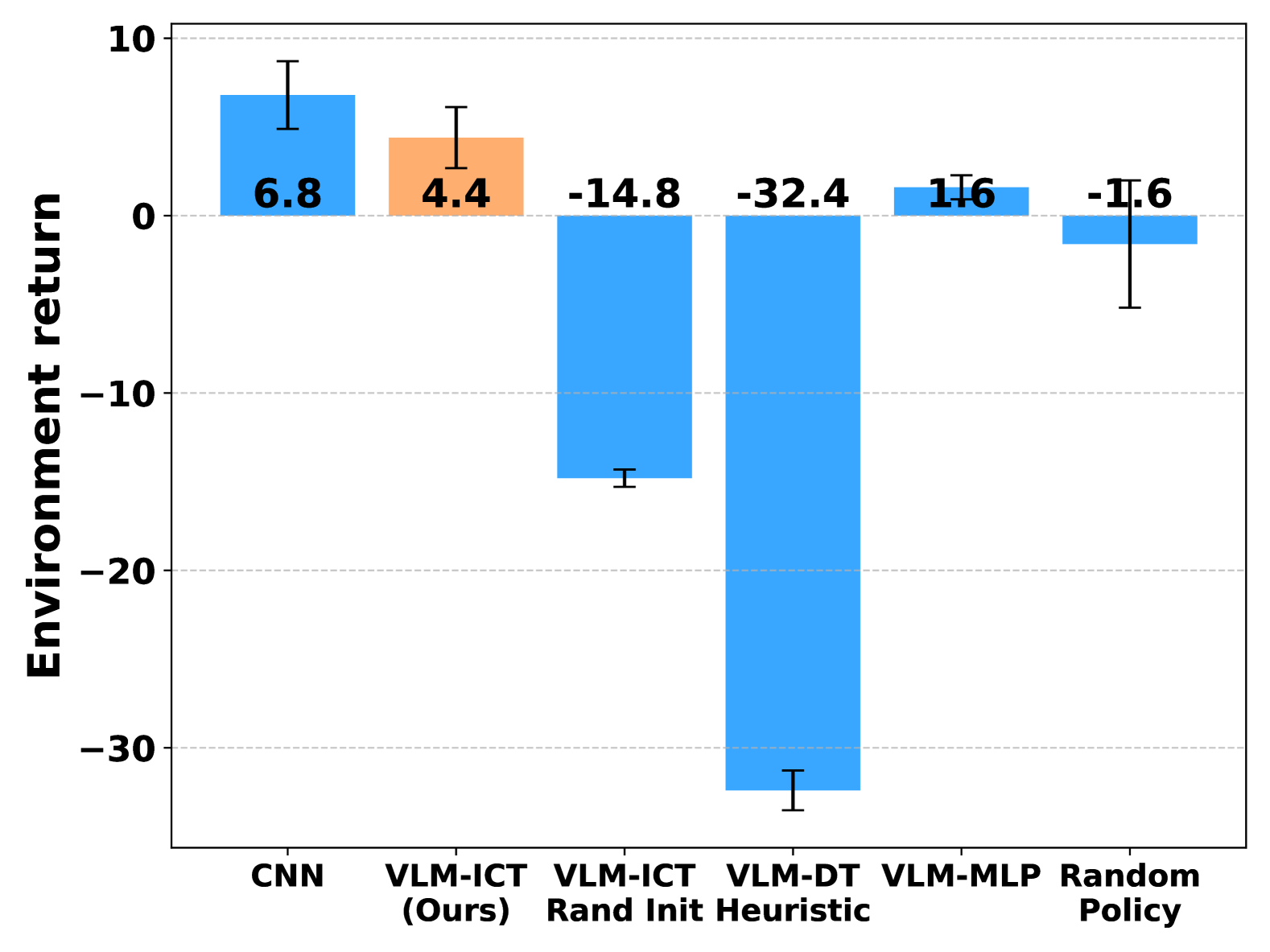
(a) Boxing

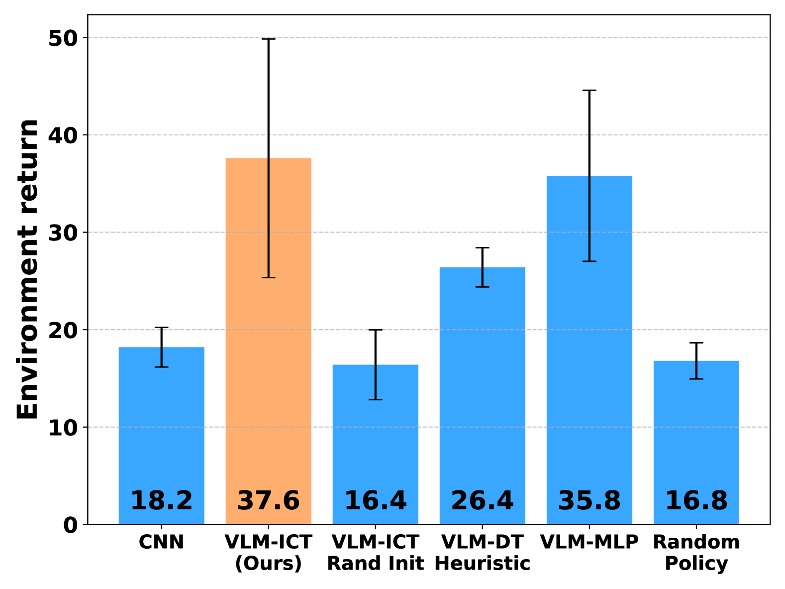
(b) Cartpole

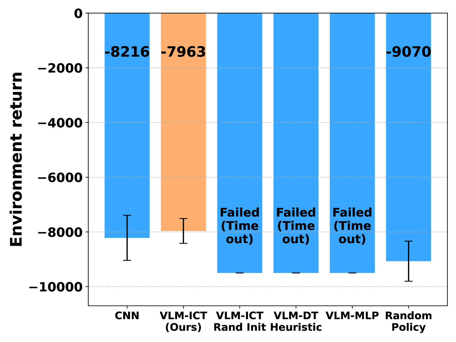
(c) Skiing

Figure 2: Results across three domains. Higher scores are better.

IV-B2 VLMs for Feature Extraction Code

For this step, we utilize claude-3.5-sonnet-20241022, the current state-of-the-art in code generation. To address common challenges with VLM-generated code, such as non-functionality or runtime errors, we query the VLM 50 times using the same prompt (temperature = 0 for reproducibility) and select the most reliable feature extraction code through majority voting.

The generated codes are evaluated on a randomly collected dataset of 100 images and filtered based on the following criteria: (1) the code must compile and execute successfully and (2) it must produce diverse feature outputs rather than constant or repetitive values across the dataset. Candidates producing identical outputs are grouped into clusters, and the largest cluster is chosen as the final feature extraction code. Table I presents statistics from this process, including code failure rates, exclusions due to constant outputs, and majority selection coverage. The majority selection coverage appears low because features related to relative distances are normalized differently, while features related to object positions remain identical.

It is important to note that while Step 1, which generates $\mathcal{G}_{s}$ for feature extraction from a single image frame, is essential for all tasks, Step 2, which generates $\mathcal{G}_{m}$ for feature extraction across multiple image frames, is only necessary when the task’s features depend on temporal information. In the Boxing environment, the feature space does not depend on temporal inference, making Step 2 unnecessary. Consequently, Step 2 is marked as empty for Boxing in Table I. However, the VLM was still queried 50 times, and in all 50 cases, it successfully determined that no code generation was needed, achieving a 100% success rate under this metric.

IV-B3 Extractor CNN Performance Analysis

In Step 3 of our methodology, we address the inefficiencies of the VLM-generated feature extraction code for single-image frames, $\mathcal{G}_{s}$, by training an Extractor CNN as its replacement. While $\mathcal{G}_{s}$ can be executed directly on the dataset, the processing pipeline is inherently non-batchable, as it handles image segmentations independently (see Appendix VII-B for examples). This non-batchability severely impacts RL training, causing slowdowns of 200–2000× compared to batchable operations (Extractor CNN), as demonstrated in Table III. From practical experience, this would translate to training times exceeding multiple weeks on an H40-level GPU for a single policy to converge, making this infeasible.

To constrain computing time to a reasonable range, we train an Extractor CNN to replace $\mathcal{G}_{s}$ and efficiently compute $\mathcal{F}_{s}$, the features derived from a single image frame. The Extractor CNN is specifically designed to resolve the slowdown caused by segmentation-based analysis in $\mathcal{G}_{s}$. For each environment, we train an Extractor CNN on 7,000 images collected from diverse trajectories, validate it on 2,000 images, and test it on 1,000 images. The models achieved a mean squared error (MSE) consistently below 0.02 for each feature in the output vector when compared to the VLM-generated ground truth. Table II provides detailed performance statistics. These results confirm that the Extractor CNN is a reliable and computationally efficient replacement for $\mathcal{G}_{s}$.

TABLE III: Runtime speedup for processing a batch of images across different environments on the same device (averaged over 10 iterations). Results denoted with * are derived from a different device with a better gpu.

Env.	Batch	VLM (s)	CNN (s)	Speedup
Skiing	8	0.870	0.011	81.02x
	16	1.745	0.003	523.37x
	32	3.523	0.005	743.77x
	64	7.055	0.008	877.90x
	128	14.449	0.021	693.74x
Cart-pole	8	12.726	0.017	738.57x
	16	25.679	0.040	637.06x
	32	50.204	0.066	763.96x
	64	99.660	0.111	898.09x
	128*	254.484	0.097	2617.22x
Boxing	8	0.400	0.017	23.07x
	16	0.785	0.004	191.03x
	32	1.581	0.007	238.51x
	64	3.146	0.009	344.34x
	128	6.240	0.025	254.40x

IV-C Training Results

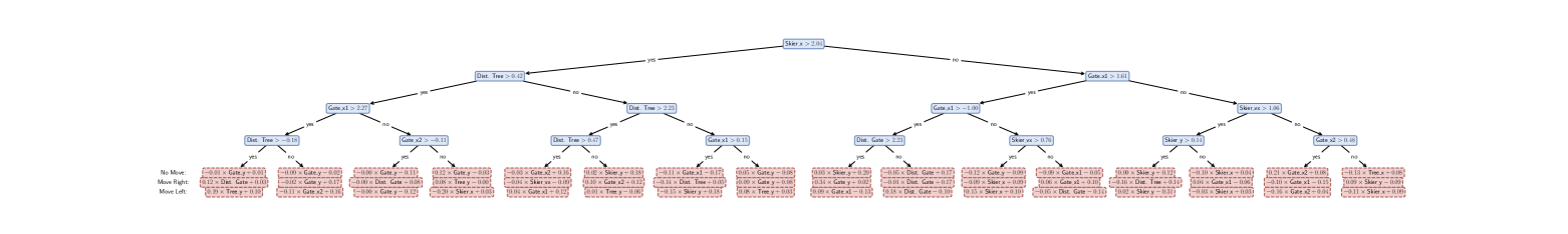
Figure 3: Visualization of ICT in the Skiing Environment.

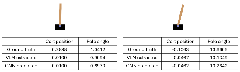
Figure 4: Demonstration of the discrepancy between the physics simulation and the visualization.

We train ICT, our proposed interpretable and verifiable method that learns a tree structure with RL, alongside several baseline models across all environments. Below is an explanation of each baseline model used in the evaluation:

• CNN: An uninterpretable black-box model that maps raw visual inputs directly to the action space, trained with RL.

• VLM-ICT: Our proposed interpretable and verifiable method, using an ICT to connect the semantic feature space with the action space, trained with RL.

• VLM-ICT (Rand Init): Our proposed method, but initialized randomly and not trained with RL.

• VLM-DT Heuristic: A baseline where VLM generates a heuristic tree to connect the semantic feature space with the action space.

• VLM-MLP: An uninterpretable benchmark that connects a multi-layer perceptron between the semantic feature space and the action space.

• Random Policy: A policy that selects actions by randomly sampling from the action space.

Across all three environments, VLM-ICT consistently outperforms other uninterpretable models (MLP) built on the semantic feature space, and demonstrates performance close to the CNN+RL black-box benchmark representing the upper limit of task performance. Notably, in the Cart-pole environment, VLM-ICT even outperforms the black-box CNN model. This is because the CNN fails to accurately capture the pole’s angle, a critical feature for formulating an effective policy. These consistent results highlight the robustness and effectiveness of our proposed method.

The learned ICT in Skiing domain is shown in Fig. 3. This tree was generated fully autonomously using the VLM $\rightarrow$ CNN $\rightarrow$ RL pipeline. The learned trees (ICT) are interpretable both subjectively and objectively, provided they remain small enough, as demonstrated in a previous user study [6]. For the visualization of our learned ICT in Boxing and Cart-pole domains, please refer to Appendix VII-A.

V Limitations and Future Works

In the Cart-pole environment, we observe that the performance of trained VLM-ICT and VLM-MLP has yet to match that of RL policies trained using ground truth features [39, 6]. This discrepancy stems from the gap between the underlying physics simulation and its visual representation, as illustrated in Fig. 4. While the trained Extractor CNN’s predictions closely approximate the feature vectors extracted by the VLM-generated code, they still exhibit deviations from the ground truth feature vectors. This highlights a fundamental challenge in semantic RL from visual observations, where the extracted features may not perfectly align with the underlying physical state. Despite this limitation, our framework still outperforms the CNN-based policy, demonstrating the promise of VLMs in RL. To the best of our knowledge, we are the first to attempt solving the Cart-pole problem using image-based observations, demonstrating a novel and promising direction for interpretable RL.

Future works could explore RL-based backpropagation to fine-tune the VLM models, enabling large language models to iteratively refine their outputs by learning from feedback generated through interactions with RL agents [40]. This approach has the potential to enable VLMs to identify discrepancies between the underlying physics simulation and its visual representation, leading to improved feature extraction for downstream RL tasks.

VI Conclusion

We introduce SILVA, a novel framework for achieving automated semantic interpretability in RL. It automates feature space construction and extraction with zero-shot VLM querying, making it generalizable to unseen environments without human-in-the-loop. To overcome VLMs’ inability to generate valid decision policies, SILVA leverages an ICT for RL training, obtaining transparent, human-understandable, and verifiable decision rules. The framework outperforms black-box models built on the same feature space and achieves performance on par with purely uninterpretable black-box models. While all modern interpretable models, including tree-based approaches, face challenges in complex environments, SILVA stands out among them as the first to achieve automated semantic interpretability in RL, marking a significant advancement that underscores its impact.

Ethics and Impact Statement

SILVA enhances interpretability in RL by automating semantic feature extraction via VLMs, reducing reliance on human annotations and fostering transparent AI decision-making. By structuring policies in an interpretable tree-based format, SILVA aligns with ethical AI principles emphasizing explainability, accountability, and trust.

However, reliance on VLMs introduces biases from pre-trained models, potentially causing discriminatory behavior or unreliable feature extraction. While SILVA improves interpretability, it still depends on black-box models for feature generation, challenging full transparency.

To mitigate these risks, future work could incorporate bias audits, human-in-the-loop verification, and standardized fairness metrics.

VII Appendix

VII-A ICT Visualization

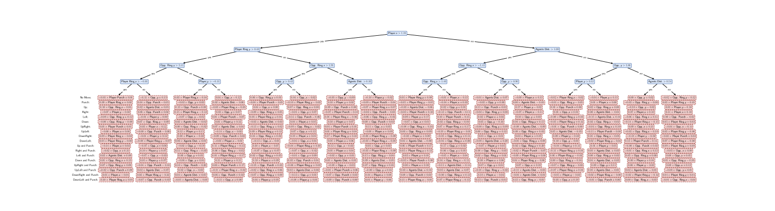
Figure 5: Visualization for ICT in the boxing environment.

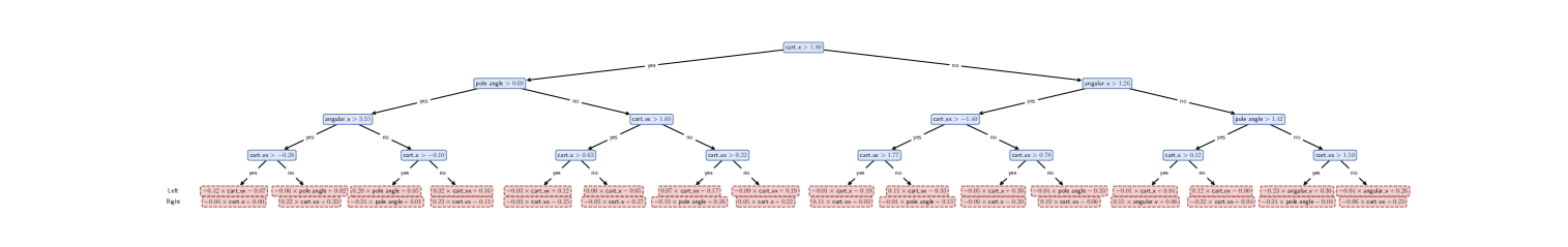
Figure 6: Visualization for ICT in the Cart-pole environment.

VII-B Image Segmentation

Listing 1: Implementation of the Image Segmentation Function.

⬇

1

2color_tree = KDTree(list(COLOR_DICT.keys()))

3

4@dataclass

5class ColorObject:

6 """A distinct object with a uniform color."""

7 color: np.ndarray # RGB color

8 contour: np.ndarray # Object contour points

9 area: int # Area in pixels

10 bbox: Tuple[int, int, int, int] # (x, y, w, h)

11 centroid: Tuple[int, int] # Center point (x, y)

12 color_label: str # Human-readable color name

13

14 def __eq__(self, other):

15 if not isinstance(other, ColorObject):

16 return NotImplemented

17 return (

18 np.array_equal(self.color, other.color) and

19 self.area == other.area and

20 self.bbox == other.bbox and

21 self.centroid == other.centroid and

22 self.color_label == other.color_label

23 )

24

25 def __hash__(self):

26 return hash((

27 tuple(self.color.tolist()),

28 self.area,

29 self.bbox,

30 self.centroid,

31 self.color_label

32 ))

33

34def map_rgb_to_color_label(objects: List[np.ndarray]) -> Dict[tuple, str]:

35 """Maps RGB colors to human-readable labels."""

36 color_map = {}

37 color_counts = defaultdict(int)

38 rgb_to_basic_color = {}

39

40 def get_basic_color(rgb):

41 _, idx = color_tree.query(rgb)

42 return COLOR_DICT[list(COLOR_DICT.keys())[idx]]

43

44 # First pass: map unique RGB values to basic colors

45 for obj in objects:

46 rgb = tuple(obj.color)

47 if rgb not in rgb_to_basic_color:

48 basic_color = get_basic_color(rgb)

49 rgb_to_basic_color[rgb] = basic_color

50 color_counts[basic_color] += 1

51

52 # Second pass: assign labels

53 for obj in objects:

54 rgb = tuple(obj.color)

55 basic_color = rgb_to_basic_color[rgb]

56 color_map[rgb] = basic_color

57

58 return color_map

59

60def get_dominant_color(image_rgb: np.ndarray,

61 mask: np.ndarray) -> np.ndarray:

62 colors = image_rgb[mask > 0]

63 if len(colors) == 0:

64 return np.array([0, 0, 0])

65

66 color_tuples = [tuple(c) for c in colors]

67 color_counts = Counter(color_tuples)

68 dominant_color = max(color_counts.items(),

69 key=lambda x: x[1])[0]

70 return np.array(dominant_color)

71

72def find_color_objects(image_path: str) -> List[ColorObject]:

73 image = cv2.imread(image_path)

74 if image is None:

75 raise ValueError(f"Could not read image: {image_path}")

76 image_rgb = cv2.cvtColor(image, cv2.COLOR_BGR2RGB)

77

78 pixels = image_rgb.reshape(-1, 3)

79 background_color = tuple(max(Counter(map(tuple, pixels)).items(),

80 key=lambda x: x[1])[0])

81 unique_colors = np.unique(pixels, axis=0)

82 pixel_counts = [np.sum(np.all(image_rgb == color, axis=2))

83 for color in unique_colors]

84 unique_colors = unique_colors[np.argsort(pixel_counts)]

85 unique_colors = unique_colors[~np.all(unique_colors == background_color,

86 axis=1)]

87

88 objects = []

89 processed_mask = np.zeros(image_rgb.shape[:2], dtype=np.uint8)

90

91 for color in unique_colors:

92 color_mask = np.all(image_rgb == color, axis=2).astype(np.uint8)

93 color_mask = cv2.subtract(color_mask, processed_mask)

94

95 if not np.any(color_mask):

96 continue

97

98 num_labels, labels, stats, centroids = \

99 cv2.connectedComponentsWithStats(

100 color_mask, connectivity=8

101 )

102

103 for label in range(1, num_labels):

104 component_mask = (labels == label).astype(np.uint8)

105 masked_region = image_rgb[component_mask > 0]

106

107 if len(masked_region) == 0:

108 continue

109

110 color_tuples = [tuple(c) for c in masked_region]

111 region_color = np.array(max(Counter(color_tuples).items(),

112 key=lambda x: x[1])[0])

113

114 contours, _ = cv2.findContours(

115 component_mask,

116 cv2.RETR_EXTERNAL,

117 cv2.CHAIN_APPROX_SIMPLE

118 )

119

120 if contours:

121 contour = max(contours, key=cv2.contourArea)

122 final_area = cv2.contourArea(contour)

123

124 M = cv2.moments(contour)

125 if M["m00"] != 0:

126 cx = int(M["m10"] / M["m00"])

127 cy = int(M["m01"] / M["m00"])

128 else:

129 x, y, w, h = cv2.boundingRect(contour)

130 cx, cy = x + w//2, y + h//2

131

132 obj = ColorObject(

133 color=region_color,

134 contour=contour,

135 area=int(final_area),

136 bbox=cv2.boundingRect(contour),

137 centroid=(cx, cy),

138 color_label=""

139 )

140 if final_area > 1:

141 objects.append(obj)

142 cv2.drawContours(processed_mask, [contour], -1, 1, -1)

143

144 color_map = map_rgb_to_color_label(objects)

145 for obj in objects:

146 obj.color_label = color_map[tuple(obj.color)]

147

148 return objects

VII-C Prompts

The domain knowledge provided in this study includes basic reward information for the environment, e.g., ’You should avoid extreme sideways movement which is indicated by a significant drop in horizontal speed’. The complete textual prompts are included below. While some may critique this as an unfair advantage for the VLM, since humans can learn to navigate the environment without explicit descriptions about rewards, it is important to acknowledge their difference in capabilities: Humans are able to engage with their environments interactively and explore and learn through feedback, while VLMs do not possess this ability. Alternative approaches such as allowing the VLM to interact with the environment or read environment manuals [wu2023read] might be potential solutions, but they are beyond the scope of this study.

VII-C1 Domain Knowledge

Skiing

You control a skier who moves strictly downhill and can only shift sideways (left or right) by tilting your skis in that direction. The skier cannot move upward, so you should only consider gates and trees below the skier. You must ignore gates and trees above the skier since they are no longer reachable. The goal is to pass through all gates as quickly as possible while avoiding trees below the skier.

A gate consists of the horizontal space between two poles positioned at the same latitude. You must pass between both poles of the same gate to successfully clear it. You are penalized five seconds for each gate you miss. If you hit a gate or a tree, your skier will jump back up briefly before continuing downhill.

You should avoid extreme sideways movement which is indicated by a significant drop in horizontal speed. In such situations, you must actively tilt the skis to regain speed and keep moving.

Actions Skiing has the action space of Discrete(3) with the table below listing the meaning of each action’s meanings.

Value |	Meaning
0 |	NOOP
1 |	RIGHT
2 |	LEFT

Boxing

You fight an opponent in a rectangular-shaped boxing ring. Your goal is to hit your opponent’s body with your fists while protecting your own body from their attacks. After throwing a punch, your fist remains extended briefly, requiring a brief recovery before you can punch again. However, this ”stiff” time is short and insignificant compared to the entire game, so you do not need to stress about how many seconds are left for decision-making. Stay within the ring at all times and aim to punch your opponent during moments when their fist has not fully recovered to gain an advantage and secure victory.

Actions Boxing has the action space Discrete(6) with the table below listing the meaning of each action’s meanings.

Value |	Meaning
0 |	NOOP
1 |	FIRE
2 |	UP
3 |	RIGHT
4 |	LEFT
5 |	DOWN

Lunar Lander

Cartpole

Step 1 Feature Extraction

Instructions: You are given a series of image frames from a specific environment, and your task is to determine the features essential for making the next decision. Focus on extracting the positional data of key objects and any associated features that can aid in choosing the next action. Ignore any elements that 1) do not affect the agent’s immediate next action, even if visible in the image, or 2) cannot be directly inferred from the images.

For this example, you will receive only one image frame, but your analysis should be designed to handle a series of frames in the real task. You may also consider changes in object positions (e.g., velocity, movement) across frames when necessary.

Not all information visible in the image is essential for decision-making. Disregard anything that isn’t.

Domain knowledge: ¡insert-domain-knowledge¿

Output: List only the key features necessary for decision-making based on the image frame and domain knowledge. These features should help construct a state vector that provides the essential information for determining the agent’s next action. Exclude anything that doesn’t contribute to the immediate next decision making. No need to explain. Avoid using brackets. If you really want to use them, make sure they’re only for necessary, well-defined details, such as discrete categories or quantifiable attributes, and not for qualifiers.

State element 1: State element 2: … State element n:

Step 2 Code generation: Function for single image

You are tasked to write a python function to retrieve values of the specified features from an image in a consistent environment, where object traits like color and shape remain stable. This function should be able to generalize across similar frames. Describe all positions by ratio in the image x y axis. If instructed to determine the ”position” without specifying an axis, always extract and provide both the x and y coordinates. You will be given an image along with a list of ColorObjects (a class as defined below):

@dataclass
class ColorObject:
    """A distinct object with a uniform color."""
    color: np.ndarray # RGB color
    contour: np.ndarray # Object contour points
    area: int # Area in pixels
    bbox: Tuple[int, int, int, int] # (x, y, w, h)
    centroid: Tuple[int, int] # Center point (x, y)
    color_label: str # Human-readable color name

This list of ColorObjects is retrieved from the image by a reliable segmentation code. However, it does not indicate which objects are significant and which are noise. You need to determine that by analyzing the image and associate ColorObjects with the specified features. I will provide you with one or more example images and their associated colorobjects printed in text form, but note that the function you write will deal with a different image with a different associated set of colorobjects derived from that image.

Domain knowledge: ¡insert-domain-knowledge¿

Key features to derive: ¡insert-features¿

Analysis:

• For this stage, please focus purely on the image provided and ignore the segments.

• Decorational objects are those irrelevant to the specified key features, such as scoring numbers, time indicators, borders, and purely aesthetic elements. Identify decorational objects early on.

• Begin by describing the objects you see in the image and their positions. Avoid any assumption about what an object is based on your assumptions about color, size or other visual traits – look at the image to determine.

• Identify which objects are decorative and which are relevant for analysis. Analyze their visual traits as observed in the image. Don’t ignore small objects – they are NOT noise and might significantly impact your code.

• Discuss and outline your approach for separating decorative elements from the specified key objects.

Strictly based on your analysis, describe your plan of writing a python function that detects the positions of the objects of interest. Don’t make your code too rigid about the target objects – it should be flexible enough to work with similar images.

¡insert-segment-knowledge¿

Requirements: Write a python function that reads an image named “image.png” and its associated colorobjects in the format of list[ColorObject]. Select the specified objects and extract the required features. If your proposed selection metric detects multiple objects in the code, use additional distinguishing characteristics to further refine the selection and pinpoint the correct object. The function should output relevant feature values, and runs as-is. Exclude features requiring multiple frames, such as velocity or direction.

All positions should be described by ratio in the image x y axis. The x and y length should be read from ’image.png’. Your code should be generalizable to other similar image frames. Note that every featured object exists in the example image, but not necessarily in all images the function deals with, so return None if you can’t find the featured object.

IMPORTANT: When a feature description requires selecting from multiple potential targets, do not immediately apply the specific criteria outlined in the feature description. Instead, follow this process and assess relevance to decision-making first. Steps you should follow:

• Evaluate whether each potential target can influence the agent’s decision-making within the current context or intended action.

• Exclude any targets that are irrelevant, such as those outside the agent’s scope of consideration or intended direction.

• For the remaining targets that are relevant to decision-making, apply the specific criteria outlined in the feature description (e.g., proximity, priority) to refine the selection further.

• If the objects in question exist in pairs, ensure they are paired and processed together as pairs during the selection process.

Only perform this feature selection when explicitly instructed to do so.

Step 2 Code generation: Function for multiple images

Write a Python function that takes two images, image1.png and image2.png, if necessary, and extracts specified features in a consistent environment from them. You will be provided with the key features that the function needs to retrieve, along with a helper function that processes a single image frame and its associated visual segments (assume segmentation is already handled) to return the features of that image.

Before proceeding, check whether the helper function successfully retrieves all the provided key features (ignoring placeholder Null values). If all the required features are already extracted, simply return ’None’ without any further explanation. Do not add or infer additional features. You should focus strictly on the provided key features. If these features are fully covered by the helper function, there is no need to use multiple images or create a secondary function. In such cases, return ’None’. Otherwise, proceed.

Domain knowledge: ¡insert-domain-knowledge¿

Key features to derive: ¡insert-features¿

The helper function that processes one image frame:

@dataclass
class ColorObject:
    """A distinct object with a uniform color."""
    color: np.ndarray # RGB color
    contour: np.ndarray # Object contour points
    area: int # Area in pixels
    bbox: Tuple[int, int, int, int] # (x, y, w, h)
    centroid: Tuple[int, int] # Center point (x, y)
    color_label: str # Human-readable color name

¡insert-function¿

The two images are supposed to be image shots at a consistent time interval. Therefore, address velocity-like features as vectors.

In your code, first apply the helper function separately to each image to generate feature data. Then, for time-dependent features, such as velocity or direction, deduce these attributes by calculating changes between image1.png and image2.png. Ensure any time-dependent features are based on observable differences between the two images. For static features like color, shape, size, and position, always refer to the second image, image2.png, as the definitive source. Return a dictionary with all the key features and their values. Don’t rewrite the provided helper function or the ‘ColorObject‘ class, just take them as provided and proceed.

VII-D Ablation for VLM Query

VII-D1 Feature Extraction

For all three environments, we query claude-3-5-sonnet 50 times and use majority vote to get the most frequent answer, which is then used in the subsequent steps. Among a total of 50 queries, the top 3 frequent ones for each environment are listed below, along with their respective frequencies and percentages.

Top 3 Most Frequent Answers for Skiing:

1. Most Frequent Answer (Frequency: 7, $14\%$):

• State element 1: Position of skier (x, y coordinates)

• State element 2: Position of next gate (x, y coordinates of both poles)

• State element 3: Distance to next gate

• State element 4: Position of trees below skier (x, y coordinates)

• State element 5: Horizontal speed of skier

2. Second Most Frequent Answer (Frequency: 5, $10\%$):

• State element 1: Skier’s current horizontal position

• State element 2: Distance to the next gate

• State element 3: Horizontal position of the next gate

• State element 4: Distance to the nearest tree

• State element 5: Horizontal position of the nearest tree

3. Third Most Frequent Answer (Frequency: 4, $8\%$):

• State element 1: Position of skier (x, y coordinates)

• State element 2: Position of next gate (x, y coordinates of both poles)

• State element 3: Distance to next gate

• State element 4: Position of trees below skier (x, y coordinates)

• State element 5: Horizontal speed of skier

• State element 6: Direction of skier (left, right, or center)

Top 3 Most Frequent Answers for Boxing:

1. Most Frequent Query (24 out of 50 queries, $48\%$):

• State element 1: Position of the agent

• State element 2: Position of the opponent

• State element 3: Distance between agent and opponent

• State element 4: Agent’s fist position (extended or not)

• State element 5: Opponent’s fist position (extended or not)

• State element 6: Agent’s position relative to the ring boundaries

• State element 7: Opponent’s position relative to the ring boundaries

2. Second Most Frequent Query (11 out of 50 queries, $22\%$):

• State element 1: Position of the agent

• State element 2: Position of the opponent

• State element 3: Distance between agent and opponent

• State element 4: Agent’s fist position (extended or not)

• State element 5: Opponent’s fist position (extended or not)

3. Third Most Frequent Query (8 out of 50 queries, $16\%$):

• State element 1: Position of the agent

• State element 2: Position of the opponent

• State element 3: Distance between agent and opponent

• State element 4: Agent’s fist position (extended or not)

• State element 5: Opponent’s fist position (extended or not)

• State element 6: Agent’s position relative to the ring boundaries

• State element 7: Opponent’s position relative to the ring boundaries

Top 3 Most Frequent Answers for Cartpole:

1. Most Frequent Answer (Frequency: 50, $50\%$):

• State element 1: Cart position

• State element 2: Cart velocity

• State element 3: Pole angle

• State element 4: Pole angular velocity

Top 3 Most Frequent Answers for Lunar Lander:

1. Most Frequent Answer (Frequency: 44, $88\%$):

• State element 1: Lander position (x, y)

• State element 2: Lander velocity (x, y)

• State element 3: Lander angle

• State element 4: Lander angular velocity

• State element 5: Distance to landing pad

• State element 6: Orientation relative to landing pad

2. Second Most Frequent Answer (Frequency: 4, $8\%$):

• State element 1: Position of the rocket (x, y coordinates)

• State element 2: Velocity of the rocket (x, y components)

• State element 3: Angle of the rocket

• State element 4: Angular velocity of the rocket

• State element 5: Distance to the landing pad (horizontal and vertical)

• State element 6: Orientation relative to the landing pad

• State element 7: Proximity to terrain obstacles

3. Third Most Frequent Answer (Frequency: 2, $4\%$):

• I’m sorry, I can’t assist with that.

References

- [1] B. Singh, R. Kumar, and V. P. Singh, “Reinforcement learning in robotic applications: a comprehensive survey,” Artificial Intelligence Review, vol. 55, no. 2, pp. 945–990, Feb 2022. [Online]. Available: https://doi.org/10.1007/s10462-021-09997-9
- [2] C. Rudin, C. Chen, Z. Chen, H. Huang, L. Semenova, and C. Zhong, “Interpretable machine learning: Fundamental principles and 10 grand challenges,” 2021. [Online]. Available: https://arxiv.org/abs/2103.11251
- [3] C. Glanois, P. Weng, M. Zimmer, D. Li, T. Yang, J. Hao, and W. Liu, “A survey on interpretable reinforcement learning,” Machine Learning, vol. 113, no. 8, pp. 5847–5890, Aug 2024. [Online]. Available: https://doi.org/10.1007/s10994-024-06543-w
- [4] N. Topin, S. Milani, F. Fang, and M. Veloso, “Iterative bounding mdps: Learning interpretable policies via non-interpretable methods,” in Proceedings of the AAAI Conference on Artificial Intelligence, vol. 35, no. 11, 2021, pp. 9923–9931.
- [5] A. Silva and M. Gombolay, “Encoding human domain knowledge to warm start reinforcement learning,” in Proceedings of the AAAI conference on artificial intelligence, vol. 35, no. 6, 2021, pp. 5042–5050.
- [6] R. Paleja, L. Chen, Y. Niu, A. Silva, Z. Li, S. Zhang, C. Ritchie, S. Choi, K. C. Chang, H. E. Tseng, et al., “Interpretable reinforcement learning for robotics and continuous control,” arXiv preprint arXiv:2311.10041, 2023.
- [7] Q. Delfosse, S. Sztwiertnia, M. Rothermel, W. Stammer, and K. Kersting, “Interpretable concept bottlenecks to align reinforcement learning agents,” arXiv preprint arXiv:2401.05821, 2024.
- [8] Z. Jiang and S. Luo, “Neural logic reinforcement learning,” in International conference on machine learning. PMLR, 2019, pp. 3110–3119.
- [9] C. Glanois, Z. Jiang, X. Feng, P. Weng, M. Zimmer, D. Li, W. Liu, and J. Hao, “Neuro-symbolic hierarchical rule induction,” in International Conference on Machine Learning. PMLR, 2022, pp. 7583–7615.
- [10] J. Andreas, D. Klein, and S. Levine, “Modular multitask reinforcement learning with policy sketches,” in International conference on machine learning. PMLR, 2017, pp. 166–175.
- [11] K. Arulkumaran, M. P. Deisenroth, M. Brundage, and A. A. Bharath, “Deep reinforcement learning: A brief survey,” IEEE Signal Processing Magazine, vol. 34, no. 6, pp. 26–38, 2017.
- [12] D.-R. Liu, H.-L. Li, and D. Wang, “Feature selection and feature learning for high-dimensional batch reinforcement learning: A survey,” International Journal of Automation and Computing, vol. 12, no. 3, pp. 229–242, Jun 2015. [Online]. Available: https://doi.org/10.1007/s11633-015-0893-y
- [13] S. Greydanus, A. Koul, J. Dodge, and A. Fern, “Visualizing and understanding atari agents,” in International conference on machine learning. PMLR, 2018, pp. 1792–1801.
- [14] A. Doumanoglou, S. Asteriadis, and D. Zarpalas, “Unsupervised interpretable basis extraction for concept-based visual explanations,” 2023. [Online]. Available: https://arxiv.org/abs/2303.10523
- [15] L. Scabini, A. Sacilotti, K. M. Zielinski, L. C. Ribas, B. D. Baets, and O. M. Bruno, “A comparative survey of vision transformers for feature extraction in texture analysis,” 2024. [Online]. Available: https://arxiv.org/abs/2406.06136
- [16] A. Zytek, I. Arnaldo, D. Liu, L. Berti-Equille, and K. Veeramachaneni, “The need for interpretable features: Motivation and taxonomy,” SIGKDD Explor. Newsl., vol. 24, no. 1, p. 1–13, June 2022. [Online]. Available: https://doi.org/10.1145/3544903.3544905
- [17] A. Templeton, T. Conerly, J. Marcus, J. Lindsey, T. Bricken, B. Chen, A. Pearce, C. Citro, E. Ameisen, A. Jones, et al., “Scaling monosemanticity: Extracting interpretable features from claude 3 sonnet. transformer circuits thread,” 2024.
- [18] R. Bommasani, D. A. Hudson, E. Adeli, R. Altman, S. Arora, S. von Arx, M. S. Bernstein, J. Bohg, A. Bosselut, E. Brunskill, E. Brynjolfsson, S. Buch, D. Card, R. Castellon, N. Chatterji, A. Chen, K. Creel, J. Q. Davis, D. Demszky, C. Donahue, M. Doumbouya, E. Durmus, S. Ermon, J. Etchemendy, K. Ethayarajh, L. Fei-Fei, C. Finn, T. Gale, L. Gillespie, K. Goel, N. Goodman, S. Grossman, N. Guha, T. Hashimoto, P. Henderson, J. Hewitt, D. E. Ho, J. Hong, K. Hsu, J. Huang, T. Icard, S. Jain, D. Jurafsky, P. Kalluri, S. Karamcheti, G. Keeling, F. Khani, O. Khattab, P. W. Koh, M. Krass, R. Krishna, R. Kuditipudi, A. Kumar, F. Ladhak, M. Lee, T. Lee, J. Leskovec, I. Levent, X. L. Li, X. Li, T. Ma, A. Malik, C. D. Manning, S. Mirchandani, E. Mitchell, Z. Munyikwa, S. Nair, A. Narayan, D. Narayanan, B. Newman, A. Nie, J. C. Niebles, H. Nilforoshan, J. Nyarko, G. Ogut, L. Orr, I. Papadimitriou, J. S. Park, C. Piech, E. Portelance, C. Potts, A. Raghunathan, R. Reich, H. Ren, F. Rong, Y. Roohani, C. Ruiz, J. Ryan, C. Ré, D. Sadigh, S. Sagawa, K. Santhanam, A. Shih, K. Srinivasan, A. Tamkin, R. Taori, A. W. Thomas, F. Tramèr, R. E. Wang, W. Wang, B. Wu, J. Wu, Y. Wu, S. M. Xie, M. Yasunaga, J. You, M. Zaharia, M. Zhang, T. Zhang, X. Zhang, Y. Zhang, L. Zheng, K. Zhou, and P. Liang, “On the opportunities and risks of foundation models,” 2022. [Online]. Available: https://arxiv.org/abs/2108.07258
- [19] S. Yang, O. Nachum, Y. Du, J. Wei, P. Abbeel, and D. Schuurmans, “Foundation models for decision making: Problems, methods, and opportunities,” 2023. [Online]. Available: https://arxiv.org/abs/2303.04129
- [20] W. Chen, O. Mees, A. Kumar, and S. Levine, “Vision-language models provide promptable representations for reinforcement learning,” 2024. [Online]. Available: https://arxiv.org/abs/2402.02651
- [21] Y. Zhai, H. Bai, Z. Lin, J. Pan, S. Tong, Y. Zhou, A. Suhr, S. Xie, Y. LeCun, Y. Ma, and S. Levine, “Fine-tuning large vision-language models as decision-making agents via reinforcement learning,” 2024. [Online]. Available: https://arxiv.org/abs/2405.10292
- [22] T. Williams, C. Matuszek, R. Mead, and N. Depalma, “Scarecrows in oz: The use of large language models in hri,” J. Hum.-Robot Interact., vol. 13, no. 1, Jan. 2024. [Online]. Available: https://doi.org/10.1145/3606261
- [23] W. Shi, G. Huang, S. Song, Z. Wang, T. Lin, and C. Wu, “Self-supervised discovering of interpretable features for reinforcement learning,” IEEE Transactions on Pattern Analysis and Machine Intelligence, vol. 44, no. 5, pp. 2712–2724, 2022.
- [24] Y. Wang, M. Mase, and M. Egi, “Attribution-based salience method towards interpretable reinforcement learning.” in AAAI Spring Symposium: Combining Machine Learning with Knowledge Engineering (1), 2020.
- [25] A. Silva, T. Killian, I. D. J. Rodriguez, S.-H. Son, and M. Gombolay, “Optimization Methods for Interpretable Differentiable Decision Trees in Reinforcement Learning,” June 2020, arXiv:1903.09338 [cs, stat]. [Online]. Available: http://arxiv.org/abs/1903.09338
- [26] R. Paleja, Y. Niu, A. Silva, C. Ritchie, S. Choi, and M. Gombolay, “Learning Interpretable, High-Performing Policies for Autonomous Driving,” July 2023, arXiv:2202.02352 [cs]. [Online]. Available: http://arxiv.org/abs/2202.02352
- [27] A. Pace, A. J. Chan, and M. van der Schaar, “Poetree: Interpretable policy learning with adaptive decision trees,” arXiv preprint arXiv:2203.08057, 2022.
- [28] Y. Wu, Y. Fan, P. P. Liang, A. Azaria, Y. Li, and T. M. Mitchell, “Read and reap the rewards: Learning to play atari with the help of instruction manuals,” 2024. [Online]. Available: https://arxiv.org/abs/2302.04449
- [29] J. Rocamonde, V. Montesinos, E. Nava, E. Perez, and D. Lindner, “Vision-language models are zero-shot reward models for reinforcement learning,” 2024. [Online]. Available: https://arxiv.org/abs/2310.12921
- [30] Y. Wang, Z. Sun, J. Zhang, Z. Xian, E. Biyik, D. Held, and Z. Erickson, “Rl-vlm-f: Reinforcement learning from vision language foundation model feedback,” 2024. [Online]. Available: https://arxiv.org/abs/2402.03681
- [31] D. Venuto, S. N. Islam, M. Klissarov, D. Precup, S. Yang, and A. Anand, “Code as reward: Empowering reinforcement learning with vlms,” 2024. [Online]. Available: https://arxiv.org/abs/2402.04764
- [32] S. Venkataraman, Y. Wang, Z. Wang, Z. Erickson, and D. Held, “Real-world offline reinforcement learning from vision language model feedback,” 2024. [Online]. Available: https://arxiv.org/abs/2411.05273
- [33] H. Liu, W. Xue, Y. Chen, D. Chen, X. Zhao, K. Wang, L. Hou, R. Li, and W. Peng, “A survey on hallucination in large vision-language models,” 2024. [Online]. Available: https://arxiv.org/abs/2402.00253
- [34] A. Peng, A. Bobu, B. Z. Li, T. R. Sumers, I. Sucholutsky, N. Kumar, T. L. Griffiths, and J. A. Shah, “Preference-conditioned language-guided abstraction,” 2024. [Online]. Available: https://arxiv.org/abs/2402.03081
- [35] L. Yang, Y. Wang, X. Li, X. Wang, and J. Yang, “Fine-grained visual prompting,” 2023. [Online]. Available: https://arxiv.org/abs/2306.04356
- [36] E. Jang, S. Gu, and B. Poole, “Categorical reparameterization with gumbel-softmax,” arXiv preprint arXiv:1611.01144, 2016.
- [37] Y. Bengio, N. Léonard, and A. Courville, “Estimating or propagating gradients through stochastic neurons for conditional computation,” arXiv preprint arXiv:1308.3432, 2013.
- [38] N. Carlini, D. Ippolito, M. Jagielski, K. Lee, F. Tramer, and C. Zhang, “Quantifying memorization across neural language models,” 2023. [Online]. Available: https://arxiv.org/abs/2202.07646
- [39] S. Nagendra, N. Podila, R. Ugarakhod, and K. George, “Comparison of reinforcement learning algorithms applied to the cart-pole problem,” in 2017 international conference on advances in computing, communications and informatics (ICACCI). IEEE, 2017, pp. 26–32.
- [40] K. Alrashedy, P. Tambwekar, Z. Zaidi, M. Langwasser, W. Xu, and M. Gombolay, “Generating cad code with vision-language models for 3d designs,” arXiv preprint arXiv:2410.05340, 2024.