Fine structure of phase diagram for social impact theory

Abstract

In this paper, the social impact theory introduced by Latané is reconsidered. A fully differentiated society is considered; that is, initially every actor has their own opinion. The equivalent of Muller’s ratchet guards that—even for the non-deterministic case (with a positive social temperature)—any opinion once removed from the opinion space does not appear again. With computer simulation, we construct the phase diagram for Latané model based on the number of surviving opinions after various evolution times. The phase diagram is constructed on the two-dimensional plane of model control parameters responsible for the effective range of interaction among actors and the social temperature. Introducing the Muller’s ratchet-like mechanism gives a non-zero chance for any opinion to be removed from the system. We believe that in such a case, for any positive temperature, ultimately a consensus is reached. However, even for a moderate system size, the time to reach consensus is very long. In contrast, for the deterministic case (without social temperature), the system may be frozen with clusters of actors having several different opinions, or even reach the cycle limit (with blinking structures).

I Introduction

The opinion dynamics remains a vivid part of sociophysics [1, 2, 3, 4]—the interdisciplinary branch of science that uses tools and methods of statistical physics to solve the problems with which sociologists fight in their everyday activities.

The models of opinion formation and dynamics [5, 6, 7] may be divided into two main groups with respect to the spectrum of opinions: with continuous or discrete opinions available in an artificial society. Among the latter, the models most studied are: voter model [8, 9, 10, 11], majority-rule model [12], Sznajd model [13] or models based on social impact [14].

The latter is based on Latané theory of social impact [15, 16]. By the way, the publication of Latané paper [16] coincides with the birth of sociophysics, which is believed to be forty years old [17]. Latané himself liked to think of this theory as ‘a light bulb theory of social relations’ [16], unintentionally making a contribution to the development of sociophysics. In this approach, every actor at the site $i$ in every discrete time step $t$ plays a role:

• of a monochrome light source (the actor illuminates others in one of $K$ available colors $\Lambda_{k}$, i.e., shows and sends opinion $\lambda_{i}(t)=\Lambda_{k}$);

• and a full-spectrum light decoder (the actor detects which color $\Lambda_{k}$ gives the highest light illuminance at the site $i$).

Based on these observed illuminances (impacts), the actors can change their opinion in the subsequent time step $(t+1)$ to that which has the strongest illuminance (impact) on them. Boltzmann-like factors yield probabilities of selecting $\Lambda_{k}$ as the opinion adopted by the agent in the $(t+1)$ time step in the non-deterministic version of algorithm [18], when the non-zero social temperature [19, 20] (information noise) is considered.

The earlier computerized model applications deal with:

• observation of a phase transition from unanimity of opinions to disordered state [21, 22];

• impact of a strong leader [23, 24] and social media influencers [25] on opinion dynamics;

• simulation of language change [26];

• modeling individual vaccination decision making [27];

• modeling bullying phenomenon in classrooms [28];

• impact of in-person closures on non-medical prescription opioid use among pupils [29], etc.

Malarz and Masłyk introduced an initially fully differentiated society [30] to Latané model, but small steps in this direction—with a system containing more than two opinions—were also made earlier for Latané model [18, 31, 32, 33, 34], voter model [35, 36, 37, 38, 39, 40, 41, 34], Sznajd model [42, 43, 44, 34], majority-rule model [45, 46, 47, 48, 49] and other [50, 51, 52, 53, 54].

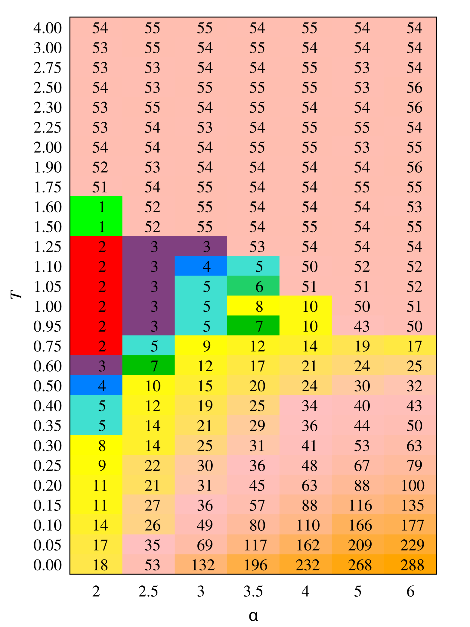
(a)

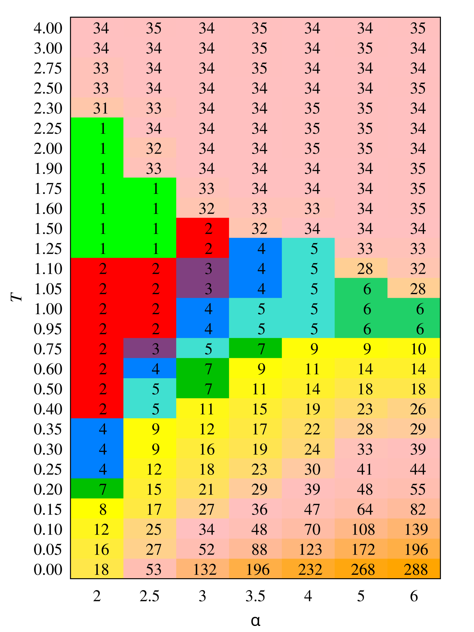
(b)

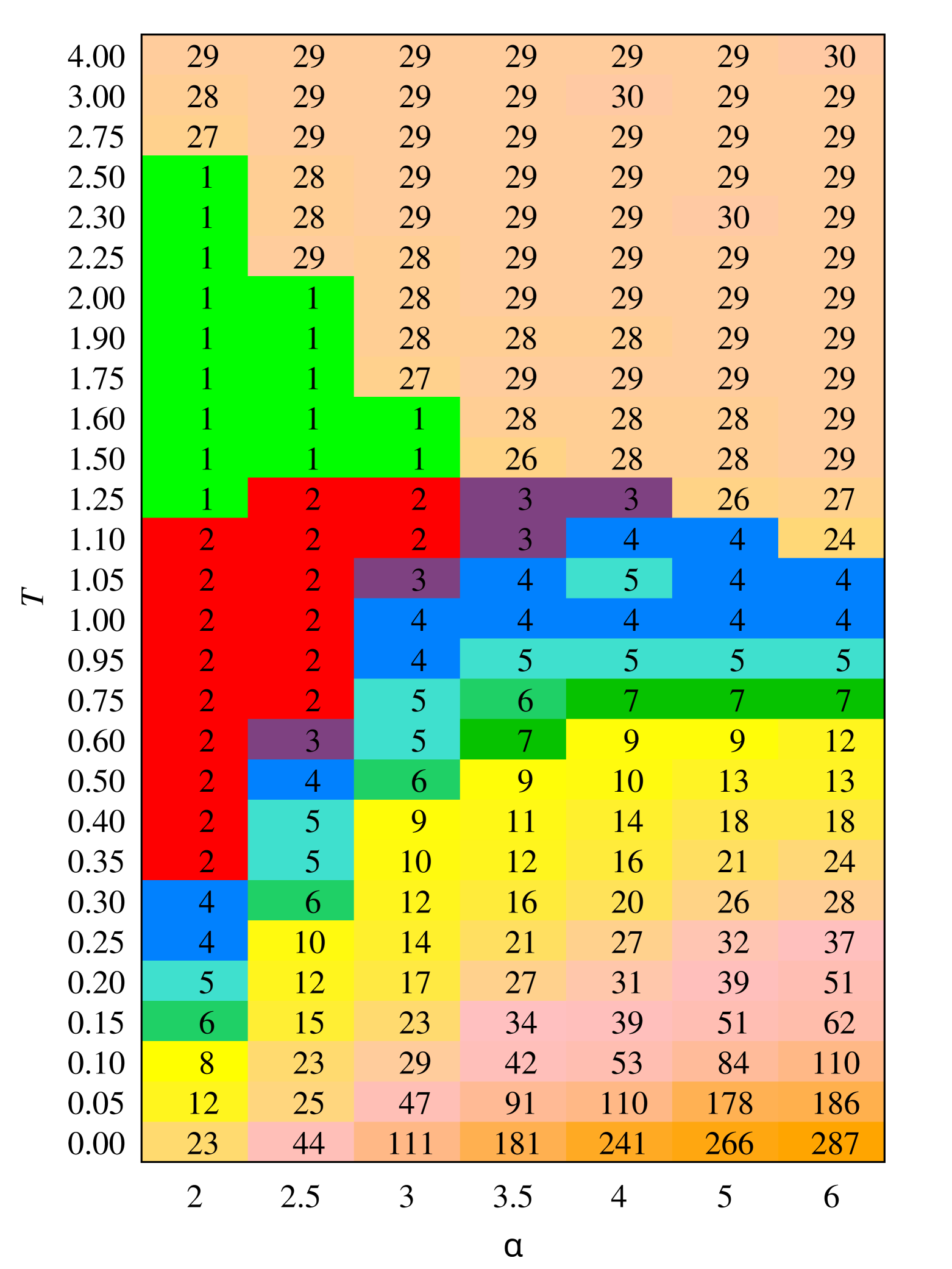
(c)

Figure 3: The largest number of surviving opinions $\max(n^{\text{u}}_{\text{o}})$ after 3(a) $t_{\textrm{max}}=10^{3}$, 3(b) $t_{\textrm{max}}=10^{5}$, 3(c) $t_{\textrm{max}}=10^{6}$ MCS. The results are gathered from $R=10^{3}$ simulations

Very recently, the preliminary shape of the phase diagram for Latené model was obtained in the $(\alpha,T)$ parameter plane [30, see Figure 3], where $\alpha$ is responsible for the effective range of interaction between actors, and social temperature $T$ measures the level of information noise.

The earlier attempts to predict this diagram were initiated in terms of:

• the size of the largest cluster [31, 33, 30];

• number of small clusters [31];

• the most probable number of surviving opinions [33];

• and the number of observed opinions [30, 34],

but also other parameters may parametrize emergent social phenomena [55].

In this paper, we return to this problem with a much more systematic approach in scanning both the model parameter responsible for the level of social noise ($T$) and the effective range of interactions ($\alpha$). The construction of the phase diagram is based solely on the number of ultimately observed (surviving) opinions. The initial number of opinions is exactly equal to the number of actors; in other words, initially every actor has their own unique opinion.

We note, however, that the meaning of the ‘phase diagram’ term in the paper title is a rather attractive marketing hook—as even defining the ordering parameter here is rather hard task [55]. In our opinion, the system governed by social impact theory tends ultimately to the consensus, (un)fortunately the time of reaching this consensus is extremely large even for relatively not too large system sizes.

II Model

We adopt the original formulation of the computerized version of the social impact model proposed by Nowak et al. [14] after its modification [18, 31, 33] to allow for a multitude of opinions $\Lambda_{k}$ and $k=1,\cdots,K$. The opinion of the actor $i$ at time $t$ is $\lambda_{i}(t)$. We assume $L^{2}$ actors that occupy nodes of the square lattice. Every actor $i$ is characterized by two parameters:

• supportiveness $s_{i}\in[0,1]$, which describes the intensity of interaction with actors currently sharing opinion $\lambda_{i}$,

• and persuasiveness $p_{i}\in[0,1]$—describing the intensity of interaction with believers of different opinions than currently adopted by the actor $i$.

The supportiveness $s_{i}$ and the persuasiveness $p_{i}$ parameters are equivalents of the powers of the light bulbs in terms of ‘a light bulb theory of social relations’ [16].

The social impact exerted on the actor $i$ by the actors $j=1,\ldots,L^{2}$, sharing the opinion $\Lambda_{k}$, is

$$\mathcal{I}_{i;k}(t)=$$

$$\quad\sum_{j=1}^{L^{2}}{\frac{4s_{j}}{g(d_{i,j})}\cdot\delta(\Lambda_{k},\lambda_{j}(t))\cdot\delta(\lambda_{j}(t),\lambda_{i}(t))}$$ (1a)

$$+\sum_{j=1}^{L^{2}}{\frac{4p_{j}}{g(d_{i,j})}\cdot\delta(\Lambda_{k},\lambda_{j}(t))\cdot[1-\delta(\lambda_{j}(t),\lambda_{i}(t))}],$$ (1b)

where $g(\cdot)$ is an arbitrarily chosen function that scales the Euclidean distance $d_{i,j}$ between agents $i$ and $j$, and the Kronecker delta $\delta(x,y)=0$ when $x\neq y$ and $\delta(x,y)=1$ when $x=y$. The combination of Kronecker deltas prevents the occurrence of terms describing the interaction between actors with different opinions in the summation (1a). Thus, we have such terms only if $\lambda_{i}(t)=\lambda_{j}(t)$, and we use actors’ supportiveness $s_{j}$ to calculate the social impact. It also prevents the appearance of terms that describe interaction between actors with the same opinions (1b) and thus we have nonzero terms only if $\lambda_{i}(t)\neq\lambda_{j}(t)$ and we use actors’ persuasiveness $p_{j}$ to calculate the social impact.

According to the social impact theory [16], the impact of the more distant actors should be smaller than that of the closest ones. Thus, the $g(\cdot)$ function should be an increasing function of its argument. Here, we assume that

$$g(x)=1+x^{\alpha},$$ (2)

where the exponent $\alpha$ is a model control parameter while the first additive component ensures finite self-supportiveness.

Dworak and Malarz showed that for $\alpha=2$, roughly 25% of the impact comes from nine nearest neighbors (when the investigated actor occupies the center of a $3\times 3$ square). This ratio increases to $\approx 59\%$, $\approx 80\%$ and $\approx 96\%$ for $\alpha=3$, 4 and 6. Calculating the relative impact exerted by actors from the neighborhood reduced to $5\times 5$ square gives roughly 39%, 76%, 92%, and 99% of the total social impact for $\alpha=2$, 3, 4, and 6, respectively [see Ref. 33, pp. 5–6, Fig. 2, Tab. 1]. Dworak and Malarz concluded that “the $\alpha$ parameter says how influential the nearest neighbors are with respect to the entire population: the larger $\alpha$, the more influential the nearest neighbors are”.

Here, we decided to use random values of $p_{i}$ and $s_{i}$. Initially, at $t=0$, each actor has their own unique opinion $\lambda_{i}(t=0)=\Lambda_{i}$.

In the deterministic version of the algorithm, social impacts (1) yield the opinion of the agent $i$ in time $(t+1)$,

$$\begin{split}\lambda_{i}(t+1)=\Lambda_{k}\\ \iff\mathcal{I}_{i,k}(t)=\max(\mathcal{I}_{i,1}(t),\mathcal{I}_{i,2}(t),\cdots,\mathcal{I}_{i,K}(t)),\end{split}$$ (3)

In other words, the actor $i$ adopts the opinion that exerts the largest social impact on them.

In the probabilistic version of the algorithm, the social impacts (1) imply Boltzmann-like probabilities

$$p_{i,k}(t)= 0 \iff\mathcal{I}_{i,k}=0$$ , (4a)

$$p_{i,k}(t)= \exp(\mathcal{I}_{i,k}(t)/T) \iff\mathcal{I}_{i,k}>0$$ , (4b)

that the actor $i$ adopts the opinion $\Lambda_{k}$. The parameter $T$ plays a role of social temperature [19, 20]. Similarly to earlier approaches [30, 34], opinions with zero impact cannot be adopted by any of the actors. In other words, according to Equation˜4a, the opinions with zero impact are not available.

Probabilities (4b) require proper normalization ensured by

$$P_{i,k}(t)=\frac{p_{i,k}(t)}{\sum^{K}_{j=1}p_{i,j}(t)}.$$ (5)

Then, the time evolution of the opinion of actor $i$ is

$$\lambda_{i}(t+1)=\Lambda_{k}\text{ with the probability }P_{i,k}(t).$$ (6)

An example of deterministic evolution for a small system (with $L^{2}=9$ actors and $K=3$ opinions) and exact calculations of social impacts are given in Appendix˜A.

III Computations

We implement Equations˜1, 2, 3, 4b, 5 and 6 as a Fortran95 code (see LABEL:lst:code in Appendix˜D). In a single Monte Carlo step (MCS), every actor has a chance to change their opinion according to Equation˜3 or Equation˜6. The system evolution takes $t_{\text{max}}$ MCS. The update of actors’ opinions is performed synchronously. The results are averaged over $R$ independent simulations, which allows for relatively easy parallelization of the computations, for example on multiple cores of the used CPU.

Figure˜1 shows the parallel speedup and calculation time for two test cases ($L=21$ and $L=51$) executed on a 32-core Intel Xeon(R) Platinum 8562Y+ CPU, with $t_{\textrm{max}}$ values chosen to have similar sequential times. The speedup $S_{q}$ for calculations running in parallel on $q$ cores is $S_{q}=t_{q}/t_{s}$, where $t_{s}$ is the sequential time (one-core calculation), and $t_{q}$ is the time of the same calculation executed on $q$ cores. For each system size, measurements were repeated three times and the averages $\bar{S}_{q}$ and $\bar{t}_{q}$ are presented in Figure˜1.

For $L=21$, the speedup is initially almost ideal, which results from the fact that all data from all threads can be stored in the cache of the processor, without the need to copy it from RAM. However, this is true only when the number of threads and used cores is below ca. 12. In the case of $L=51$, even a single thread requires a large amount of memory, beyond the available cache of the CPU, which results in the speedup characteristics typical for Amdahl’s law [56].

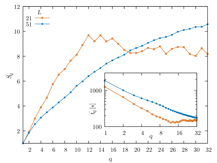
Figure 1: Average speedup $\bar{S}_{q}$ of the used code running in parallel on $q$ cores for $L=21$ with $t_{\textrm{max}}=10^{4}$ and $L=51$ with $t_{\textrm{max}}=10$; calculations consisting of $R=1680$ simulations repeated three times to obtain the average value. The inset shows the corresponding average wall-clock times $\bar{t}_{q}$ in a log-log plot

IV Results

The simulations are carried out on a square lattice with open boundary conditions and with size $L=21$, that is, for an artificial society of 441 actors. We assume random values of $s_{i}$ and $p_{i}$ taken uniformly from the interval $[0,1]$.

In Figure˜2 the phase diagram of the Latané model is presented in the $(\alpha,T)$ parameter plane. The different colors of ‘bricks’ and different numerical sequences on them correspond to different final (that is, at the time $t=t_{\text{max}}$) states of the system observed in simulation. The presence of number ‘1’ in a sequence informs on the possibility of observation of opinion unanimity; ‘2’—on system polarization; ‘3’, ‘4’ and ‘5’—on

$$n_{\text{o}}^{\text{u}}\equiv n_{\text{o}}(t\to\infty)$$ (7)

equal to 3, 4, and 5, respectively. The ‘6’ indicates that finally more than five opinions were observed ($n_{\text{o}}^{\text{u}}>5$). The mixture of labels, for instance ‘12’, indicates co-existence of phases ‘1’ and ‘2’, ‘1234’, indicates co-existence of phases ‘1’, ‘2’, ‘3’ and ‘4’, etc. The subsequent diagrams show the evolution of the system after $t_{\text{max}}=10^{3}$ [Figure˜2(a)], $t_{\text{max}}=10^{5}$ [Figure˜2(b)] and $t_{\text{max}}=10^{6}$ [Figure˜2(c)] MCS.

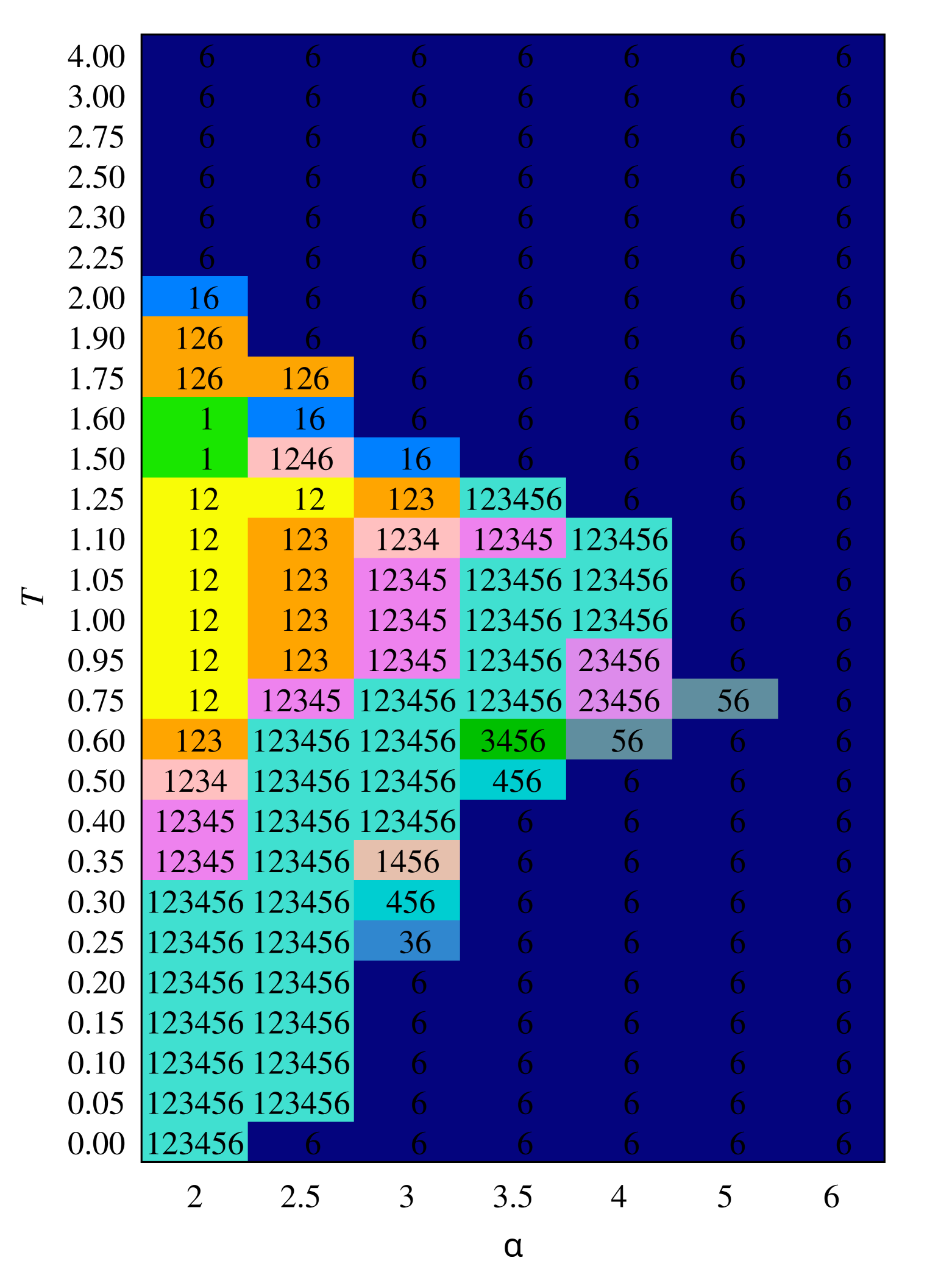
(a)

(b)

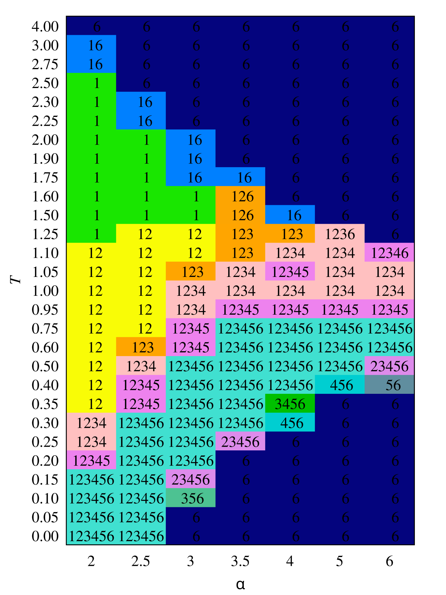
(c)

Figure 2: Phase diagram of Latané model: ‘1’ = unanimity; ‘2’ = polarization; ‘3’ = three opinions; ‘4’ = four opinions; ‘5’ = five opinions; ‘6’ = more than five opinions; ‘12’ = co-existence phases 1 and 2; ‘16’ = co-existence phases 1 and 6; ‘1234’ = co-existence phases 1, 2, 3, 4; ‘12345’ = co-existence phases 1, 2, 3, 4, 5; ‘123456’ = co-existence phases 1, 2, 3, 4, 5, 6, etc. The results are gathered from $R=10^{3}$ simulations. In subsequent diagrams evolution after 2(a) $t_{\text{max}}=10^{3}$, 2(b) $t_{\text{max}}=10^{5}$, 2(c) $t_{\text{max}}=10^{6}$ MCS are presented

In Figure˜3 the largest numbers $\max(n^{\text{u}}_{\text{o}})$ of surviving opinions after $t_{\textrm{max}}=10^{3}$ [Figure˜3(a)], $t_{\textrm{max}}=10^{5}$ [Figure˜3(b)], $t_{\textrm{max}}=10^{6}$ [Figure˜3(c)] are presented. This allows us to distinguish various system behaviors and provide more detailed information on the final state of the system when the label ‘6’ is indicated in the phase diagram given in Figure˜2.

Figure˜4 shows frequency $f$ (in per mille) of ultimately surviving $n_{\textrm{o}}^{\textrm{u}}$ opinions obtained in $R=10^{3}$ simulations after performing $t_{\textrm{max}}=10^{5}$ MCS. The subsequent figures indicate frequencies for $n_{\textrm{o}}^{\textrm{u}}=1$ [Figure˜4(a)], $n_{\textrm{o}}^{\textrm{u}}=2$ [Figure˜4(b)], $n_{\textrm{o}}^{\textrm{u}}=3$ [Figure˜4(c)], $n_{\textrm{o}}^{\textrm{u}}=4$ [Figure˜4(d)], $n_{\textrm{o}}^{\textrm{u}}=5$ [Figure˜4(e)] and $n_{\textrm{o}}^{\textrm{u}}>5$ [Figure˜4(f)].

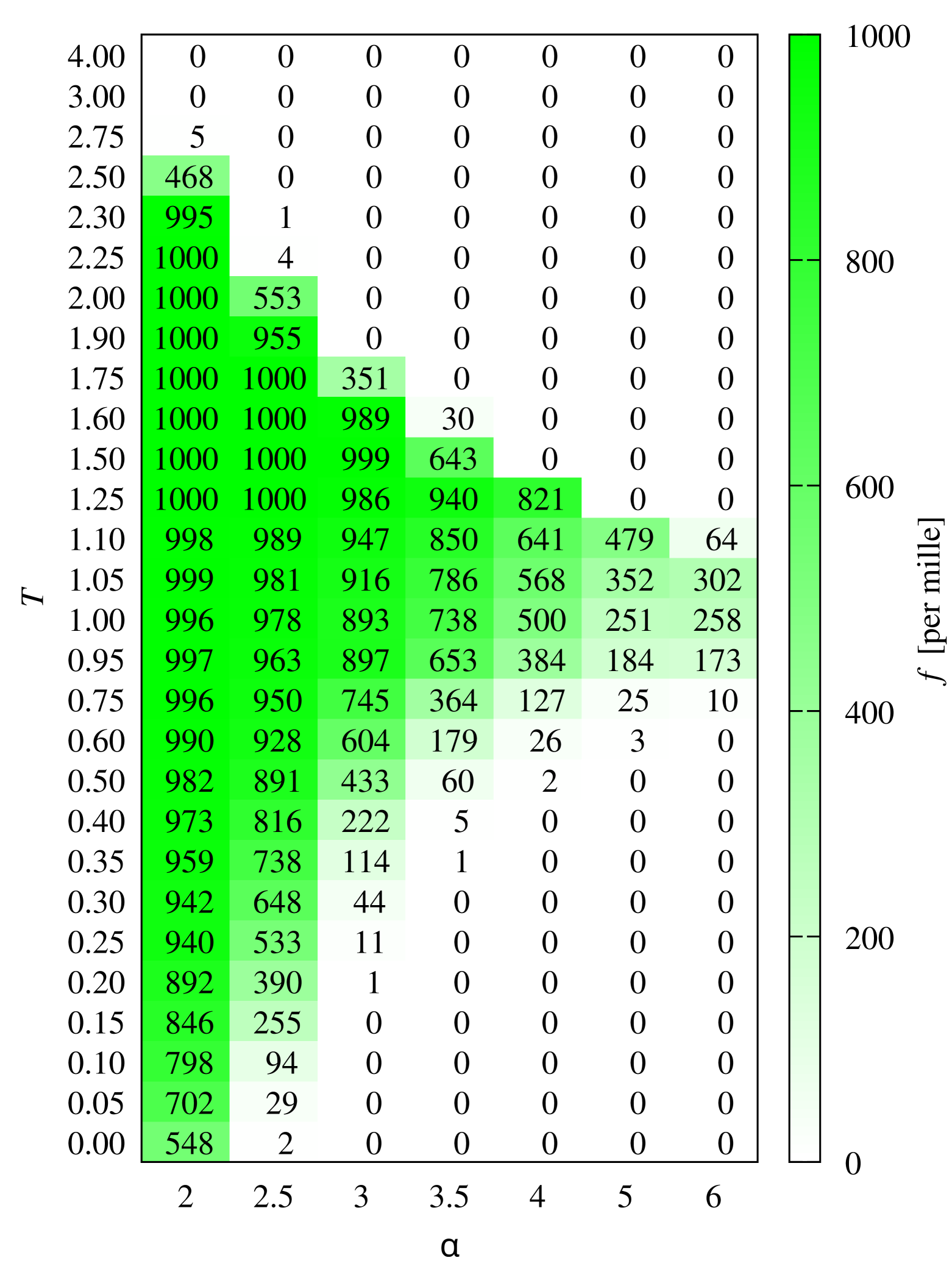
(a) $n_{\text{o}}^{\textrm{u}}=1$

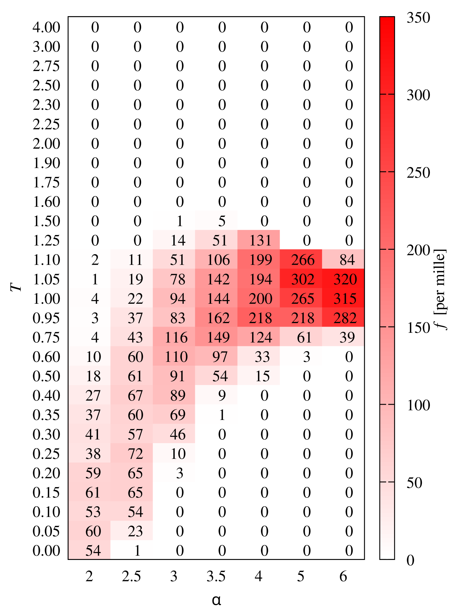
(b) $n_{\text{o}}^{\textrm{u}}=2$

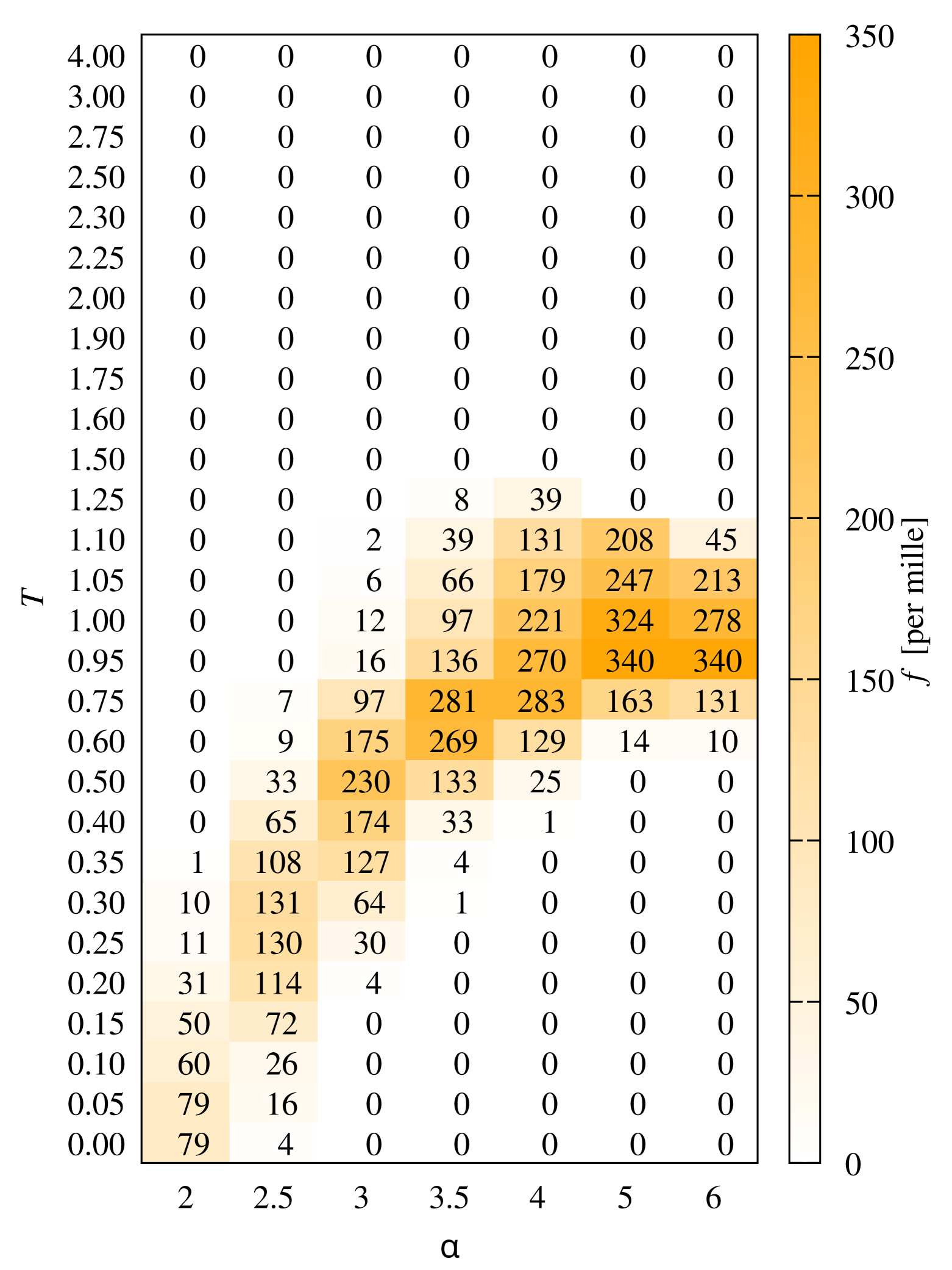
(c) $n_{\text{o}}^{\textrm{u}}=3$

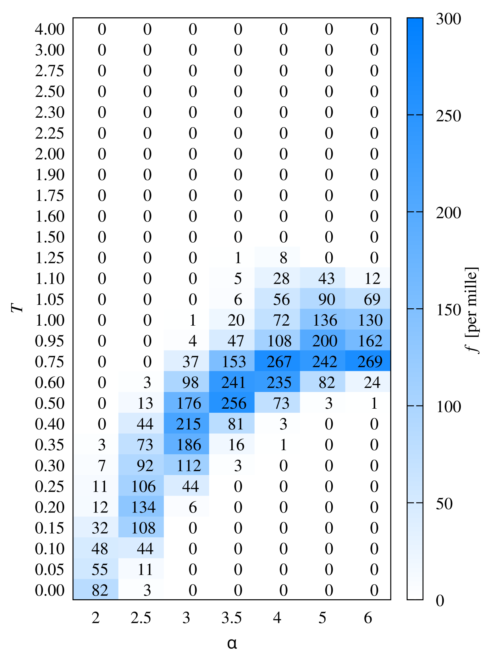
(d) $n_{\text{o}}^{\textrm{u}}=4$

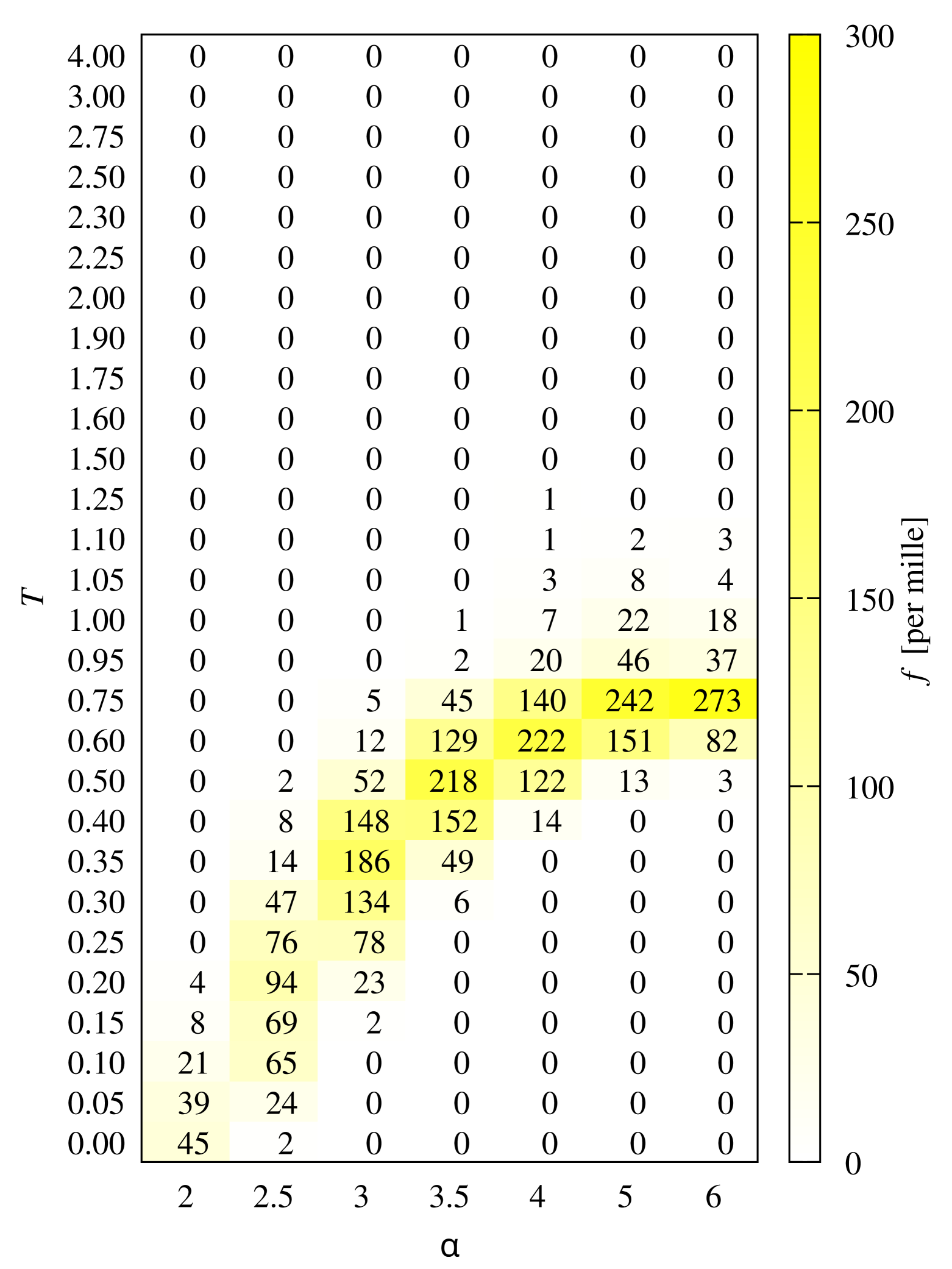
(e) $n_{\text{o}}^{\textrm{u}}=5$

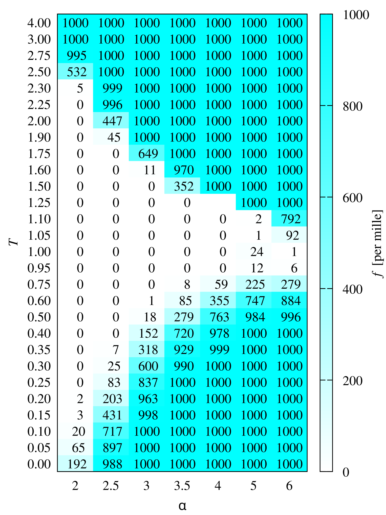
(f) $n_{\text{o}}^{\textrm{u}}>5$

Figure 4: Frequency $f$ (in per mille) of ultimately surviving $n_{\textrm{o}}^{\textrm{u}}$ opinions. 4(a) $n_{\textrm{o}}^{\textrm{u}}=1$, 4(b) 2, 4(c) 3, 4(d) 4, 4(e) 5 and 4(f) more than 5. The results are gathered from $R=10^{3}$ simulations after completing $t_{\textrm{max}}=10^{5}$ MCS

The detailed distributions of $n_{\textrm{o}}^{\text{u}}$ as functions of the social temperature $T$ for various parameters $\alpha$ after $t_{\textrm{max}}=10^{3}$ (see Figure˜9), $t_{\textrm{max}}=10^{5}$ (see Figure˜10) and $t_{\textrm{max}}=10^{6}$ (see Figure˜11) are presented in Appendix˜B.

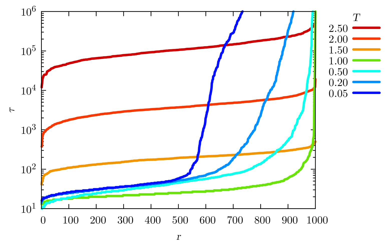
(a) $\alpha=2$

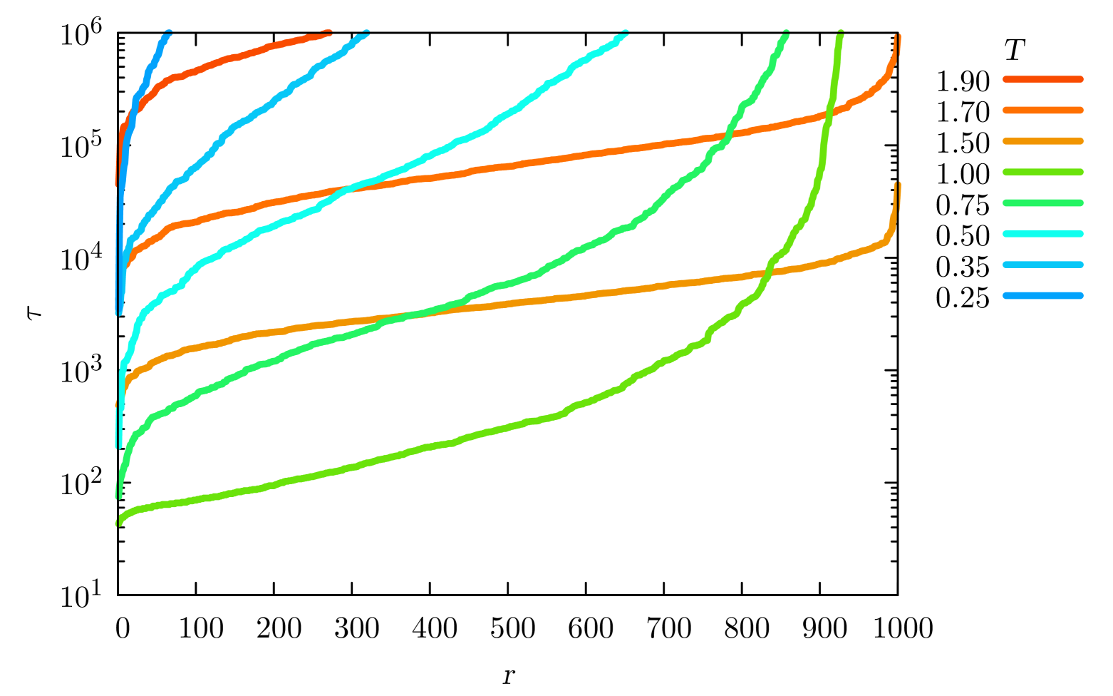
(b) $\alpha=3$

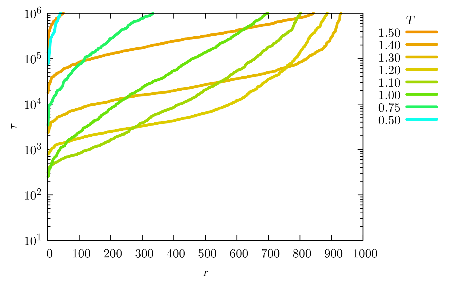
(c) $\alpha=4$

Figure 5: Examples of the time $\tau$ of reaching the consensus ($n_{\text{o}}^{\text{u}}=1$) as dependent on the number $r$ of the performed simulation (ranked in ascending order) for 5(a) $\alpha=2$, 5(b) $\alpha=3$, 5(c) $\alpha=4$ and various temperatures $T$ after $t_{\textrm{max}}=10^{6}$

V Discussion

In Figure˜2 we can observe the time evolution of the phase diagram for the social impact model. During this evolution, subsequently the area covered with bricks labeled with ‘1’ increases while area covered with bricks labeled ‘6’ decreases. This tendency is also reflected in Figure˜3, as the area covered by bricks labeled ‘1’, ‘2’ and ‘3’ increases at the expense of reducing the volume of bricks with higher labels. This means a subsequent reduction of the number of opinions available in the system. Unfortunately (for computational sociologists), the rate of this reduction is very slow: The snapshots of the phase diagram presented in Figures˜2(a) and 2(c) [and also in Figures˜3(a) and 3(c)] are separated by three orders of magnitude in the simulation time $t_{\textrm{max}}$.

In Figure˜4 we see details of the phase diagram presented in Figure˜2(b) in terms of the frequency $f$ (in per mille) of ultimately surviving $n_{\textrm{o}}^{\textrm{u}}$ opinions after completing $t_{\textrm{max}}=10^{5}$ MCS for $n_{\textrm{o}}^{\textrm{u}}=1$ [Figure˜4(a)], $n_{\textrm{o}}^{\textrm{u}}=2$ [Figure˜4(b)], $n_{\textrm{o}}^{\textrm{u}}=3$ [Figure˜4(c)], $n_{\textrm{o}}^{\textrm{u}}=4$ [Figure˜4(d)], $n_{\textrm{o}}^{\textrm{u}}=5$ [Figure˜4(e)] and more than five opinions ($n_{\textrm{o}}^{\textrm{u}}\geq 6$) [Figure˜4(f)]. As we can see in Figure˜4(a) the social temperature $T\approx 1$ is conducive to reaching consensus as we observe $f>0$ even for $\alpha>4$. On the other hand, the comparison of Figure˜4(a), Figure˜4(b) and Figure˜4(c) shows that for $0.95\leq T\leq 1$ and $5\leq\alpha\leq 6$ the chance of system polarization outperforms the chance of reaching consensus although surviving of three opinions in this region is the most probable.

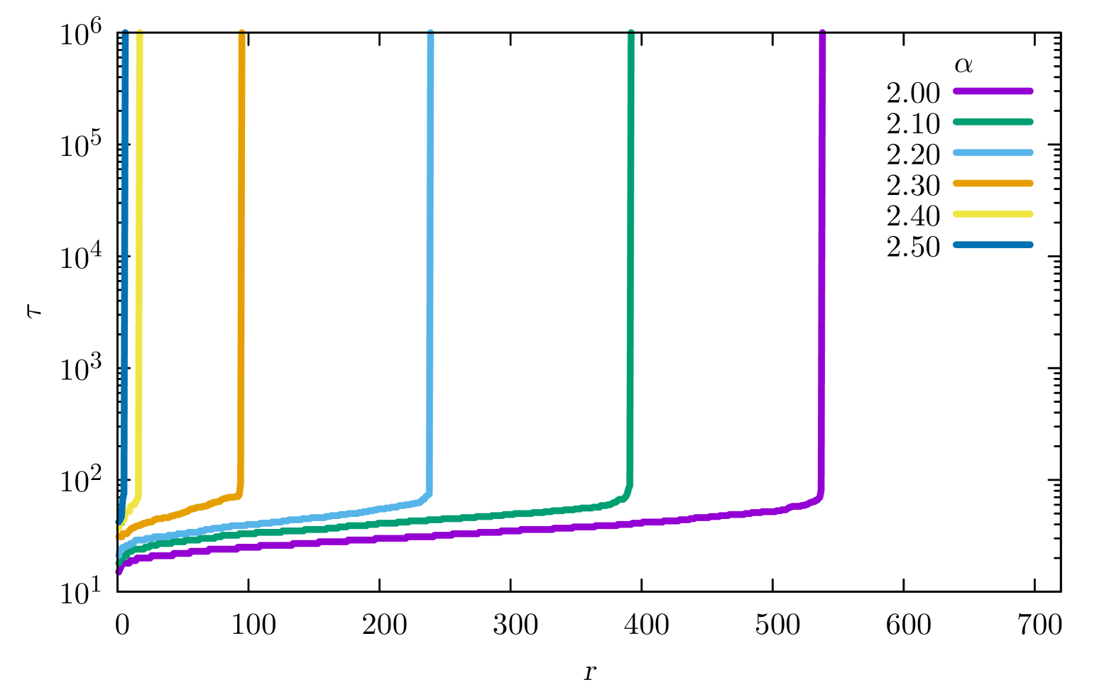
(a)

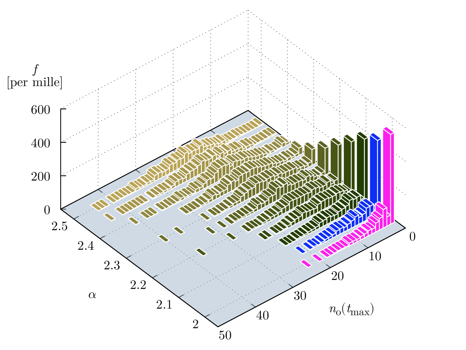
(b)

Figure 6: 6(a) The time $\tau$ of reaching the consensus as dependent on the number $r$ of the performed simulation (ranked in ascending order) for various values of $\alpha$. 6(b) Distribution of $n^{\textrm{u}}_{\textrm{o}}$. For both sub-figures the deterministic case is considered ($T=0$). The simulations are carried out for $L=21$, until $t_{\textrm{max}}=10^{6}$ MCS are performed and the results are averaged over $R=1000$ simulations

Figure˜5 shows time $\tau$ of reaching the consensus as dependent on the number of simulations (here with numeric label $r$ of the simulation sorted accordingly to the increasing time $\tau$ of reaching the consensus) for $\alpha=2$ [Figure˜5(a)], $\alpha=3$ [Figure˜5(b)], $\alpha=4$ [Figure˜5(c)] and various temperatures $T$. As we can see, the times $\tau$ of reaching consensus are limited by the assumed maximal simulation time (here $t_{\textrm{max}}=10^{6}$) for $\alpha=2$ and $T<1$ [Figure˜5(a)], $\alpha=3$ except for $1.5<T<1.7$ [Figure˜5(b)] and for all temperatures $T$ presented for $\alpha=4$ [Figure˜5(c)]. The similar restriction of time to reach the consensus $\tau\leq t_{\textrm{max}}=10^{6}$ is also observed for the deterministic version of the algorithm (for $T=0$) as presented in Figure˜6(a) for various values of $\alpha$. The fraction of simulations leading to $\tau\leq t_{\textrm{max}}=10^{6}$ monotonically decreases with the effective range of interactions expressed by the values of $\alpha$. This is even more apparent in Figure˜6(b), where the distribution of $n^{\textrm{u}}_{\textrm{o}}$ is presented. The increase in the parameter $\alpha$ reduces the effective range of interaction, which successfully improves the chance of reaching a consensus.

In the non-deterministic case ($T>0$), for a finite system (finite $L$) the presence of Muller’s ratchet in the model rules [restriction (4a)] makes the probability of any opinion vanishing finite. In principle, it is only a matter of time that just one opinion survives. However, the time to reach the consensus in Latané model seems to be extremely long. When Muller’s ratchet is excluded from the model rules [absence of restriction (4a)], at high temperatures ($T\to\infty$) the appearance of every opinion $\Lambda_{k}$ becomes equally probable, and its abundance in the system in the limit of $t\to\infty$ is $L^{2}/K$ [18].

In the deterministic version of the algorithm ($T=0$) the situation is quite opposite: the stable (long-lived states) of the system with $n^{\textrm{u}}_{\textrm{o}}>1$ are possible as shown by Lewenstein et al. in Reference 57. Examples of such states are presented in Figure˜12 in Appendix˜C.

Therefore, at the lowest temperatures ($T\to 0$) we observe remnants of this stability and a multitude of observed opinions. However, even after $10^{6}$ MCS the non-zero probability of changes in the state of the system is observed. In Figure˜13 in Appendix˜C we show examples of maps of opinions for $t_{\textrm{max}}=10^{6}$ (in the left column) and associated probabilities $P$ of sustaining opinions (in the right column). As one may expect, these probabilities are finite ($P<1$) at the boundaries between various opinions.

It seems that the most intriguing result is the insensibility of the largest number of surviving opinions ($\approx 55$, 34 and 29 for $t_{\text{max}}=10^{3}$, $10^{5}$ and $10^{6}$, respectively) on the parameters $\alpha$ and $T$ when they are high enough (see upper right corners in Figure˜3). The border line of appearance of these numbers on the maps presented in Figure˜3 is also clearly visible on the maps of frequencies $f$ of ultimately surviving opinions (Figure˜4) for $n^{\text{u}}_{\text{o}}=1$ [Figure˜4(a)] and $n^{\text{u}}_{\text{o}}>5$ [Figure˜4(f)] but totally undetectable for maps for $2\leq n^{\text{u}}_{\text{o}}\leq 5$ [Figures˜4(b), 4(c), 4(d) and 4(e)].

VI Conclusion

In this paper, the opinion dynamics model based on the social impact theory of Latané enriched with Muller’s ratchet is reconsidered. With computer simulation, we check the time evolution of the phase diagram for this model, when the fully differentiated society at initial time is assumed (that is, every actor starts with their own opinion).

When the observation time $t_{\text{max}}$ increases, consensus is reached in a systematically wider range of parameters $(\alpha,T)$. However, this consensus is only partial in some cases, depending on the exact position in the $(\alpha,T)$-space. Except for the lowest studied values of the parameter $\alpha$ the characteristic pattern of the thermal evolution is observed: for both low and high temperature the phase labeled ‘6’ prevails. However, the sources of this prevalence have totally different grounds. For low values of $T$ the system is ‘frozen’ far from consensus, while for high temperatures the Boltzmann-like factors (4b) for selecting any of still available opinions become roughly equal, although the number of available opinions decreases.

It is clear that the possibility of reaching consensus is limited only by the assumed simulation time $t_{\text{max}}$ (in our case set to $10^{3}$, $10^{5}$ and $10^{6}$ MCS). The further extension of this time, let us say for next decade, that is up to $t_{\text{max}}=10^{7}$—even for such moderate system size as $L^{2}=441$ agents—excludes possibility of accomplishing simulations in a reasonable real-world time, even with parallelization of code and access to TOP500 most powerful supercomputers. In our opinion, the system governed by the theory of social impact in the presence of finite social temperature $T>0$ ultimately tends to consensus. However, the time to reach this consensus is extremely long even for relatively small system sizes.

In contrast to earlier approaches [18, 31, 33], in this study we maintain the genetically motivated sociological equivalent of Muller’s ratchet [58, 59] introduced in Reference 30. As we deal with finite-size systems, the probability of vanishing of any opinion $\Lambda_{k}$ ($k=1,\cdots,K$) available in the system is also finite. In other words, it is only a matter of time when all—except one—opinions will disappear, and ultimately the consensus will take place. In contrast, for the deterministic version stable clusters of various opinions emerge.

After $t_{\textrm{max}}=10^{5}$ MCS for $\alpha=6$ and $1\leq T\leq 1.05$, and also for $\alpha=5$ and $T=1$, we observe $f(n_{\textrm{o}}^{\textrm{u}}=2)>f(n_{\textrm{o}}^{\textrm{u}}=1)$, which means that in this range of parameters the system polarization is more probable than reaching consensus. We conclude that the intermediate social noise $T\approx 1$ and low effective range of interaction $\alpha>4$ favor opinion polarization in society.

Appendix A Examples of small system evolution

(a)

(b)

Figure 7: Example of agents’ 7(a) persuasiveness $p_{x,y}$ and 7(b) supportiveness $s_{x,y}$ for small system of nine agents

Let us calculate some impacts $\mathcal{I}$ for a toy system of nine actors with $K=3$ opinions marked ‘red’ ($R$), ‘green’ ($G$) and ‘blue’ ($B$) and perform step-by-step system evolution with the deterministic version of the algorithm ($T=0$). Actors’ supportiveness $s_{x,y}$ and persuasiveness $p_{x,y}$ are indicated on Figure˜7. We assume $\alpha=2$ in the distance scaling function (2). Here, $\mathcal{I}_{(x,y);C}$ represents the social impact on the actor in the position $(x,y)$ exerted by the actors who have the opinion $C$. Let us start with calculation of the social impact exerted by believers of each opinion available in the system at three arbitrarily selected positions $(1,1)$, $(1,3)$ and $(3,3)$. Initially, at $t=0$, the actors have opinions presented in Figure˜8(a).

According to Equation˜1a, the impact of (the single) believer of opinion $B$ at position $(3,3)$ and at time $t=0$ is

$$\mathcal{I}_{(3,3);B}=4\left(\frac{s_{3,3}}{1+d_{(3,3);(3,3)}^{2}}\right)=\frac{4\cdot 0.1}{1+0^{2}}=0.4$$ (8)

(since any single believer has no more supporters than themself) and at coordinates $(1,1)$, $(1,3)$—according to Equation˜1b

$$\mathcal{I}_{(1,1);B}=4\left(\frac{p_{3,3}}{1+d_{(3,3);(1,1)}^{2}}\right)=\frac{4\cdot 0.9}{1+(2\sqrt{2})^{2}}=0.4,$$ (9)

and

$$\mathcal{I}_{(1,3);B}=4\left(\frac{p_{3,3}}{1+d_{(3,3);(1,3)}^{2}}\right)=\frac{4\cdot 0.9}{1+2^{2}}=0.72.$$ (10)

The impacts on these three positions by other opinions (‘red’ and ‘green’) at time $t=0$ are

$$\begin{split}\mathcal{I}_{(3,3);R}=4\left(\frac{p_{1,3}}{1+d_{(3,3);(1,3)}^{2}}+\frac{p_{1,1}}{1+d_{(3,3);(1,1)}^{2}}+\frac{p_{2,1}}{1+d_{(3,3);(2,1)}^{2}}+\frac{p_{3,1}}{1+d_{(3,3);(3,1)}^{2}}\right)\\ =4\left(\frac{0.3}{1+2^{2}}+\frac{0.1}{1+(2\sqrt{2})^{2}}+\frac{0.4}{1+\sqrt{5}^{2}}+\frac{0.7}{1+2^{2}}\right)\approx 1.11,\end{split}$$ (11)

$$\begin{split}\mathcal{I}_{(3,3);G}=4\left(\frac{p_{2,3}}{1+d_{(3,3);(2,3)}^{2}}+\frac{p_{1,2}}{1+d_{(3,3);(1,2)}^{2}}+\frac{p_{2,2}}{1+d_{(3,3);(2,2)}^{2}}+\frac{p_{3,2}}{1+d_{(3,3);(3,2)}^{2}}\right)\\ =4\left(\frac{0.6}{1+1^{2}}+\frac{0.2}{1+\sqrt{5}^{2}}+\frac{0.5}{1+\sqrt{2}^{2}}+\frac{0.8}{1+1^{2}}\right)=3.6,\end{split}$$ (12)

$$\begin{split}\mathcal{I}_{(1,1);R}=4\left(\frac{s_{1,1}}{1+d_{(1,1);(1,1)}^{2}}+\frac{s_{1,3}}{1+d_{(1,1);(1,3)}^{2}}+\frac{s_{2,1}}{1+d_{(1,1);(2,1)}^{2}}+\frac{s_{3,1}}{1+d_{(1,1);(3,1)}^{2}}\right)\\ =4\left(\frac{0.9}{1+0^{2}}+\frac{0.7}{1+2^{2}}+\frac{0.6}{1+1^{2}}+\frac{0.3}{1+2^{2}}\right)=5.6,\end{split}$$ (13)

$$\begin{split}\mathcal{I}_{(1,1);G}=4\left(\frac{p_{1,2}}{1+d_{(1,1);(1,2)}^{2}}+\frac{p_{2,2}}{1+d_{(1,1);(2,2)}^{2}}+\frac{p_{2,3}}{1+d_{(1,1);(2,3)}^{2}}+\frac{p_{3,2}}{1+d_{(1,1);(3,2)}^{2}}\right)\\ =4\left(\frac{0.2}{1+1^{2}}+\frac{0.5}{1+\sqrt{2}^{2}}+\frac{0.6}{1+\sqrt{5}^{2}}+\frac{0.8}{1+\sqrt{5}^{2}}\right)=2,\end{split}$$ (14)

$$\begin{split}\mathcal{I}_{(1,3);R}=4\left(\frac{s_{1,3}}{1+d_{(1,3);(1,3)}^{2}}+\frac{s_{1,1}}{1+d_{(1,3);(1,1)}^{2}}+\frac{s_{2,1}}{1+d_{(1,3);(2,1)}^{2}}+\frac{s_{3,1}}{1+d_{(1,3);(3,1)}^{2}}\right)\\ =4\left(\frac{0.7}{1+0^{2}}+\frac{0.9}{1+2^{2}}+\frac{0.6}{1+\sqrt{5}^{2}}+\frac{0.3}{1+\sqrt{8}^{2}}\right)\approx 4.05,\end{split}$$ (15)

$$\begin{split}\mathcal{I}_{(1,3);G}=4\left(\frac{p_{1,2}}{1+d_{(1,3);(1,2)}^{2}}+\frac{p_{2,2}}{1+d_{(1,3);(2,2)}^{2}}+\frac{p_{3,2}}{1+d_{(1,3);(3,2)}^{2}}+\frac{p_{2,3}}{1+d_{(1,3);(2,3)}^{2}}\right)\\ =4\left(\frac{0.2}{1+1^{2}}+\frac{0.5}{1+\sqrt{2}^{2}}+\frac{0.8}{1+\sqrt{5}^{2}}+\frac{0.6}{1+1^{2}}\right)=2.8.\end{split}$$ (16)

Thus, in the next step the actors at positions $(1,1)$ and $(1,3)$ will sustain their ‘red’ opinion as $\mathcal{I}_{(1,1);R}>\mathcal{I}_{(1,1);G}>\mathcal{I}_{(1,1);B}$ and $\mathcal{I}_{(1,3);R}>\mathcal{I}_{(1,3);G}>\mathcal{I}_{(1,3);B}$. In contrast, the actor at position $(3,3)$ will change their opinion from ‘blue’ to ‘green’—as $\mathcal{I}_{(3,3);G}>\mathcal{I}_{(3,3);R}>\mathcal{I}_{(3,3);B}$.

The subsequent time steps (up to $t=5$) are presented in the following rows of Figure˜8. The first column shows the time evolution of the opinions $\lambda_{(x,y)}$ of agents at sites $(x,y)$, while the second, third, and fourth columns indicate social impacts $\mathcal{I}_{(x,y);C}$ for opinions $C$ (here colored as: ‘red’, ‘green’ and ‘blue’), respectively.

At $t=1$ the impacts on ‘red’ actor at position $(3,1)$ are

$$\mathcal{I}_{(3,1);B}=0,$$ (17)

$$\begin{split}\mathcal{I}_{(3,1);R}=4\left(\frac{s_{1,1}}{1+d_{(3,1);(1,1)}^{2}}+\frac{s_{2,1}}{1+d_{(3,1);(2,1)}^{2}}+\frac{s_{3,1}}{1+d_{(3,1);(3,1)}^{2}}+\frac{s_{1,3}}{1+d_{(3,1);(1,3)}^{2}}\right)\\ =4\left(\frac{0.9}{1+2^{2}}+\frac{0.6}{1+1^{2}}+\frac{0.3}{1+0^{2}}+\frac{0.7}{1+(2\sqrt{2})^{2}}\right)\approx 3.43,\end{split}$$ (18)

$$\begin{split}\mathcal{I}_{(3,1);G}=4\left(\frac{p_{1,2}}{1+d_{(3,1);(1,2)}^{2}}+\frac{p_{2,2}}{1+d_{(3,1);(2,2)}^{2}}+\frac{p_{3,2}}{1+d_{(3,1);(3,2)}^{2}}+\frac{p_{2,3}}{1+d_{(3,1);(2,3)}^{2}}+\frac{p_{3,3}}{1+d_{(3,1);(3,3)}^{2}}\right)\\ =4\left(\frac{0.2}{1+\sqrt{5}^{2}}+\frac{0.5}{1+\sqrt{2}^{2}}+\frac{0.8}{1+1^{2}}+\frac{0.6}{1+\sqrt{5}^{2}}+\frac{0.9}{1+2^{2}}\right)=3.52\end{split}$$ (19)

and as $\mathcal{I}_{(3,1);G}>\mathcal{I}_{(3,1);R}>\mathcal{I}_{(3,1);B}$ the actor at site $(3,1)$ changes their opinion from ‘red’ (Figure˜8(e)) to ‘green’ (Figure˜8(i)).

At $t=2$ the impacts on ‘red’ actor at position $(2,1)$ are

$$\mathcal{I}_{(2,1);B}=0,$$ (20)

$$\begin{split}\mathcal{I}_{(2,1);R}=4\left(\frac{s_{1,1}}{1+d_{(2,1);(1,1)}^{2}}+\frac{s_{2,1}}{1+d_{(2,1);(2,1)}^{2}}+\frac{s_{1,3}}{1+d_{(2,1);(1,3)}^{2}}\right)\\ =4\left(\frac{0.9}{1+1^{2}}+\frac{0.6}{1+0^{2}}+\frac{0.7}{1+\sqrt{5}^{2}}\right)\approx 4.67,\end{split}$$ (21)

$$\begin{split}\mathcal{I}_{(2,1);G}=4\left(\frac{p_{3,1}}{1+d_{(2,1);(3,1)}^{2}}+\frac{p_{1,2}}{1+d_{(2,1);(1,2)}^{2}}+\frac{p_{2,2}}{1+d_{(2,1);(2,2)}^{2}}+\frac{p_{3,2}}{1+d_{(2,1);(3,2)}^{2}}+\frac{p_{2,3}}{1+d_{(2,1);(2,3)}^{2}}+\frac{p_{3,3}}{1+d_{(2,1);(3,3)}^{2}}\right)\\ =4\left(\frac{0.7}{1+1^{2}}+\frac{0.2}{1+\sqrt{2}^{2}}+\frac{0.5}{1+1^{2}}+\frac{0.8}{1+\sqrt{2}^{2}}+\frac{0.6}{1+2^{2}}+\frac{0.9}{1+\sqrt{5}^{2}}\right)\approx 4.81\end{split}$$ (22)

and as $\mathcal{I}_{(2,1),G}>\mathcal{I}_{(2,1),R}>\mathcal{I}_{(2,1),B}$ the actor at site $(2,1)$ changes their opinion from ‘red’ (Figure˜8(i)) to ‘green’ (Figure˜8(m)).

At $t=3$ the impacts on ‘red’ actor at position $(1,3)$ are

$$\mathcal{I}_{(1,3);B}=0,$$ (23)

$$\begin{split}\mathcal{I}_{(1,3);R}=4\left(\frac{s_{1,3}}{1+d_{(1,3);(1,3)}^{2}}+\frac{s_{1,1}}{1+d_{(1,1);(1,3)}^{2}}\right)=4\left(\frac{0.7}{1+0^{2}}+\frac{0.9}{1+2^{2}}\right)=3.52,\end{split}$$ (24)

$$\begin{split}\mathcal{I}_{(1,3);G}=4\Bigg{(}\frac{p_{2,1}}{1+d_{(1,3);(2,1)}^{2}}+\frac{p_{3,1}}{1+d_{(1,3);(2,3)}^{2}}+\frac{p_{1,2}}{1+d_{(1,3);(1,2)}^{2}}+\frac{p_{2,2}}{1+d_{(1,3);(2,2)}^{2}}+\\ \frac{p_{3,2}}{1+d_{(1,3);(3,2)}^{2}}+\frac{p_{2,3}}{1+d_{(1,3);(2,3)}^{2}}+\frac{p_{3,3}}{1+d_{(1,3);(3,3)}^{2}}\Bigg{)}\\ =4\left(\frac{0.4}{1+\sqrt{5}^{2}}+\frac{0.7}{1+(2\sqrt{2})^{2}}+\frac{0.2}{1+1^{2}}+\frac{0.5}{1+\sqrt{2}^{2}}+\frac{0.8}{1+\sqrt{5}^{2}}+\frac{0.6}{1+1^{2}}+\frac{0.9}{1+2^{2}}\right)\approx 4.10\end{split}$$ (25)

and as $\mathcal{I}_{(1,3);G}>\mathcal{I}_{(1,3);R}>\mathcal{I}_{(1,3);B}$ the actor at site $(1,3)$ changes their opinion from ‘red’ (Figure˜8(m)) to ‘green’ (Figure˜8(q)).

At $t=4$ the impacts on ‘red’ actor at position $(1,1)$ are

$$\mathcal{I}_{(1,1);B}=0,$$ (26)

$$\begin{split}\mathcal{I}_{(1,1);R}=4\left(\frac{s_{1,1}}{1+d_{(1,1);(1,1)}^{2}}\right)=4\left(\frac{0.9}{1+0^{2}}\right)=3.6,\end{split}$$ (27)

$$\begin{split}\mathcal{I}_{(1,1);G}=4\Bigg{(}\frac{p_{2,1}}{1+d_{(1,1);(2,1)}^{2}}+\frac{p_{2,3}}{1+d_{(1,1);(2,3)}^{2}}+\frac{p_{1,2}}{1+d_{(1,1);(1,2)}^{2}}+\frac{p_{2,2}}{1+d_{(1,1);(2,2)}^{2}}+\\ \frac{p_{3,2}}{1+d_{(1,1);(3,2)}^{2}}+\frac{p_{1,3}}{1+d_{(1,1);(1,3)}^{2}}+\frac{p_{2,3}}{1+d_{(1,1);(2,3)}^{2}}+\frac{p_{3,3}}{1+d_{(1,1);(3,3)}^{2}}\Bigg{)}\\ =4\left(\frac{0.4}{1+1^{2}}+\frac{0.7}{1+2^{2}}+\frac{0.2}{1+1^{2}}+\frac{0.5}{1+\sqrt{2}^{2}}+\frac{0.8}{1+\sqrt{5}^{2}}+\frac{0.3}{1+2^{2}}+\frac{0.6}{1+\sqrt{5}^{2}}+\frac{0.9}{1+(2\sqrt{2})^{2}}\right)=4\end{split}$$ (28)

and as $\mathcal{I}_{(1,1);G}>\mathcal{I}_{(1,1);R}>\mathcal{I}_{(1,1);B}$ the actor at site $(1,1)$ changes their opinion from ‘red’ [Figure˜8(q)] to ‘green’ [Figure˜8(u)].

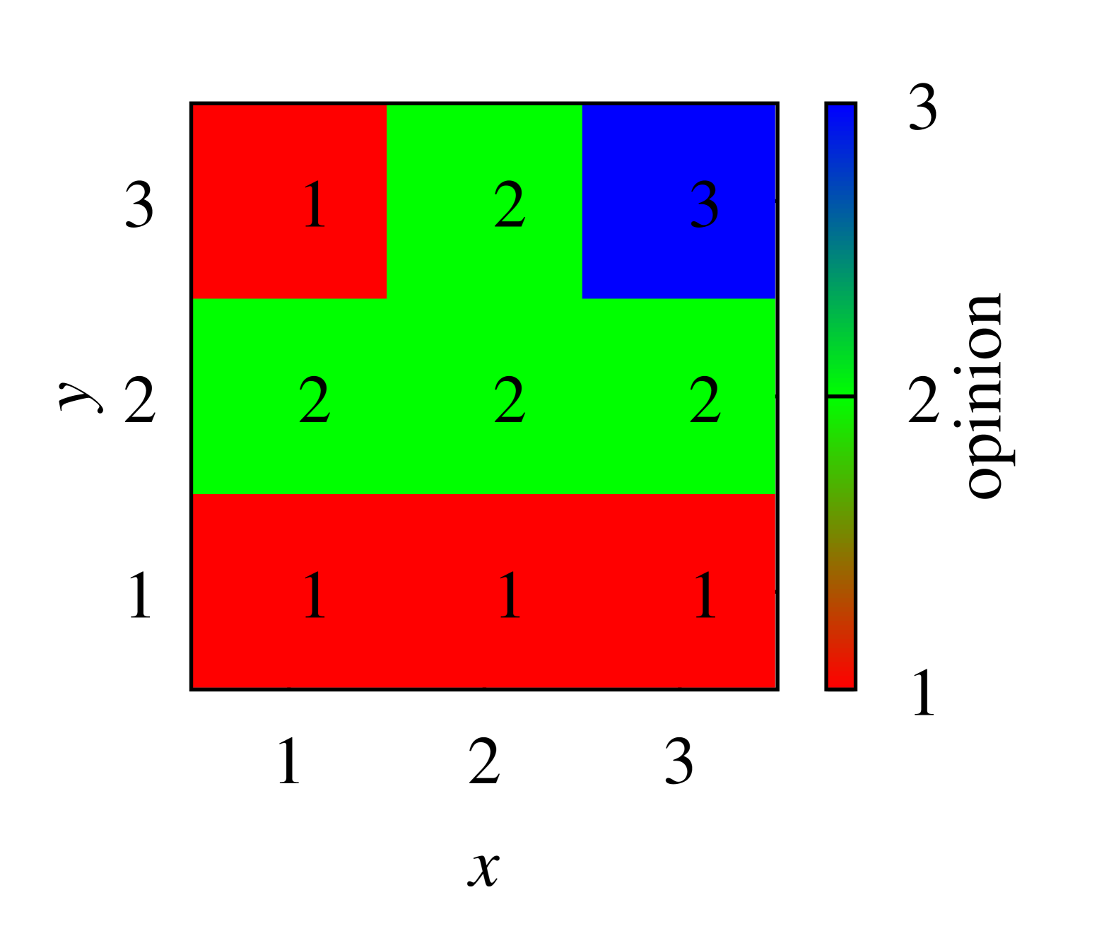
(a) $\lambda_{(x,y)}$, $t=0$

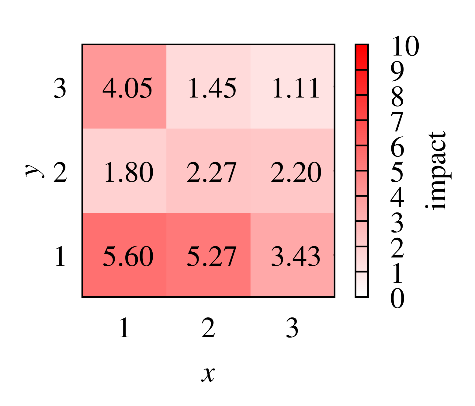
(b) $\mathcal{I}_{(x,y),R}$, $t=0$

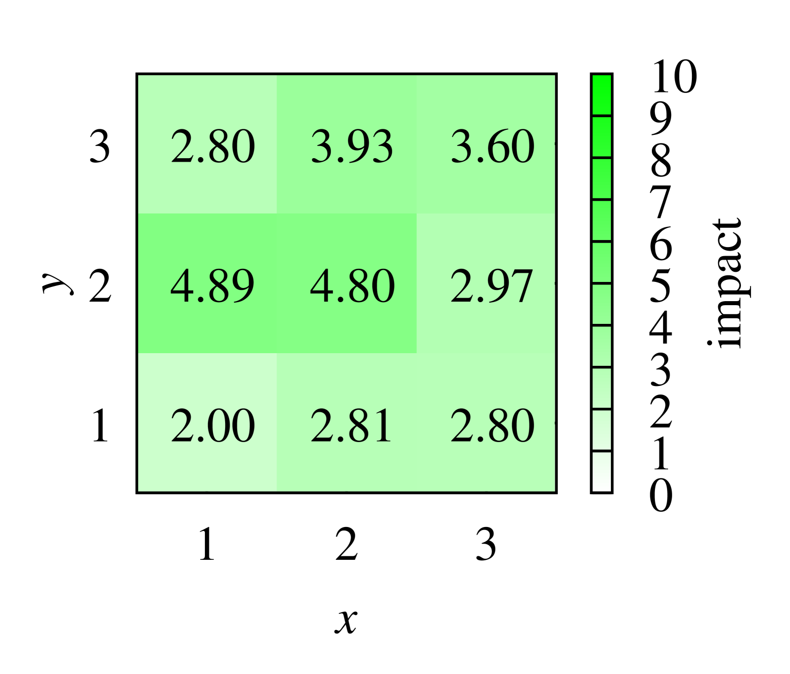
(c) $\mathcal{I}_{(x,y),G}$, $t=0$

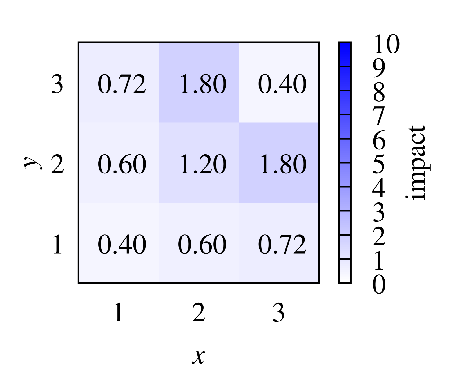
(d) $\mathcal{I}_{(x,y),B}$, $t=0$

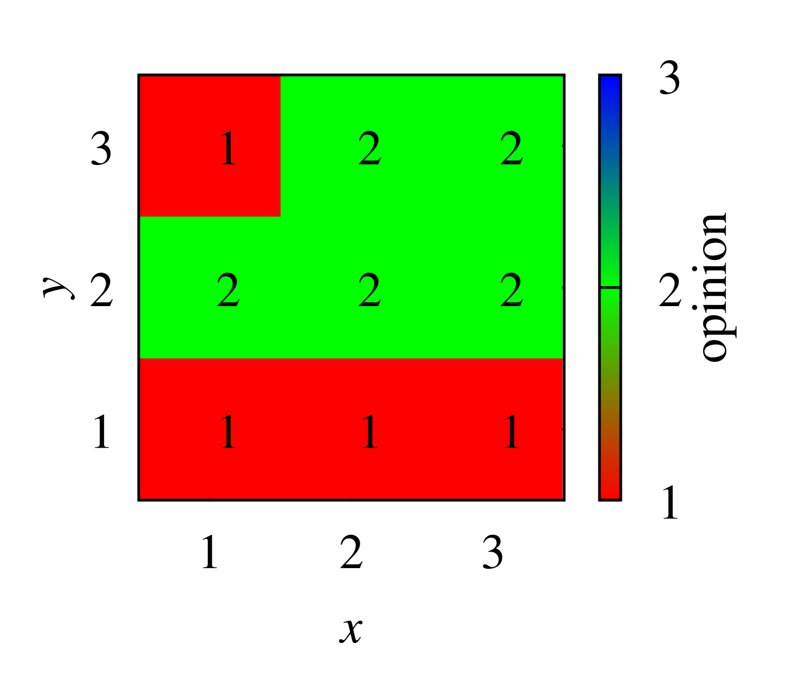
(e) $\lambda_{(x,y)}$, $t=1$

(f) $\mathcal{I}_{(x,y),R}$, $t=1$

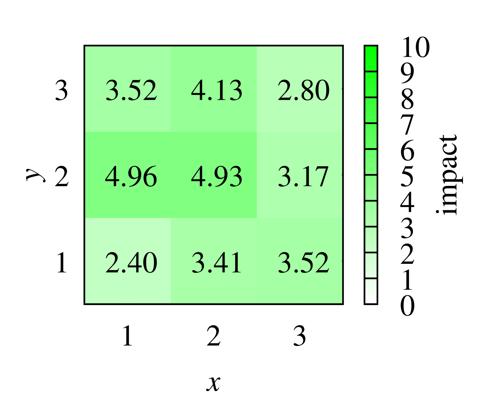
(g) $\mathcal{I}_{(x,y),G}$, $t=1$

(h) $\mathcal{I}_{(x,y),B}$, $t=1$

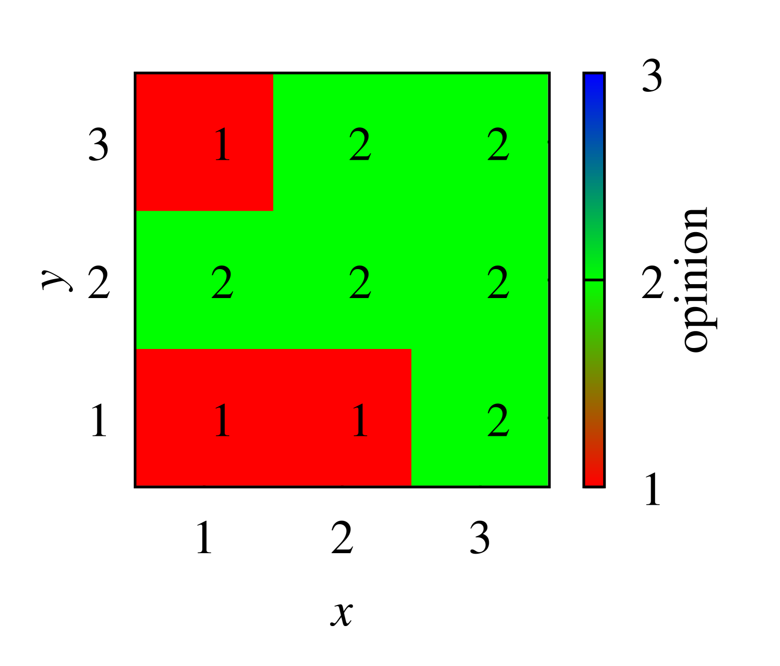
(i) $\lambda_{(x,y)}$, $t=2$

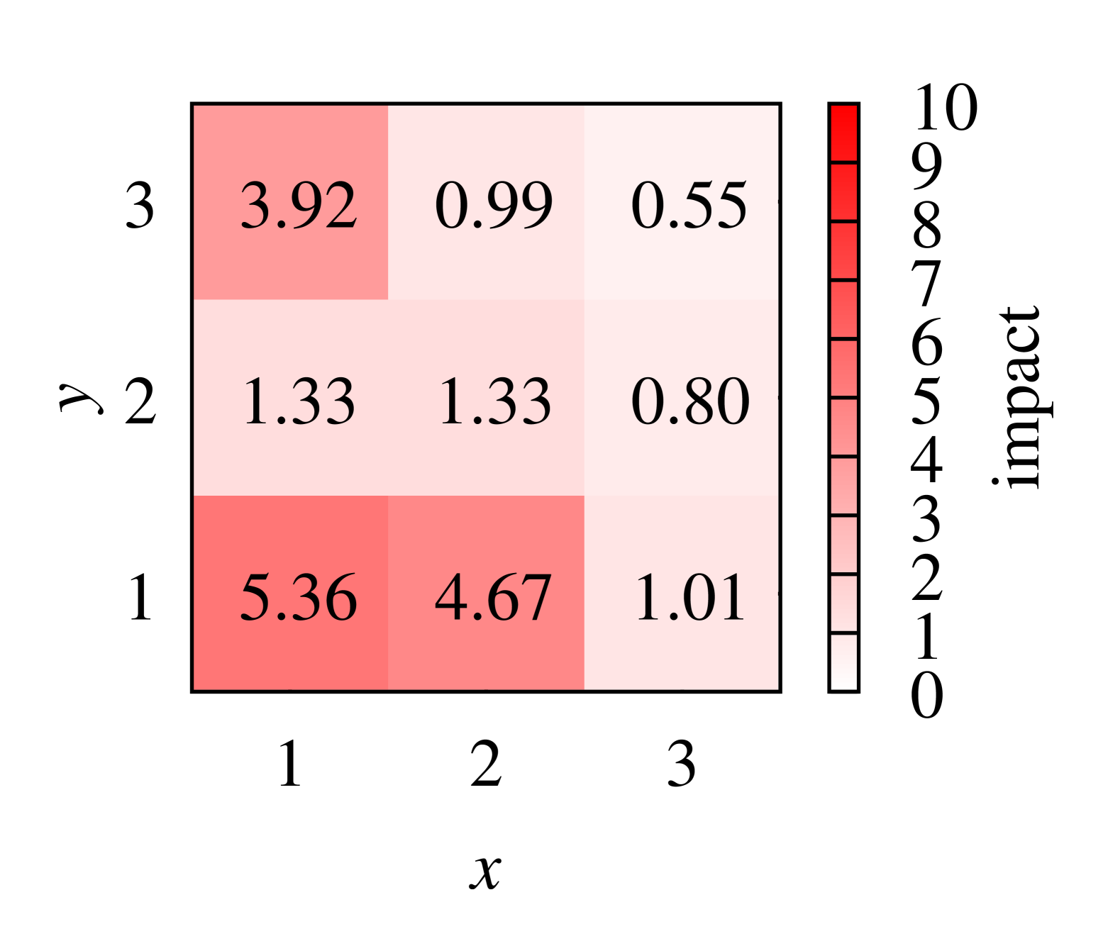
(j) $\mathcal{I}_{(x,y),R}$, $t=2$

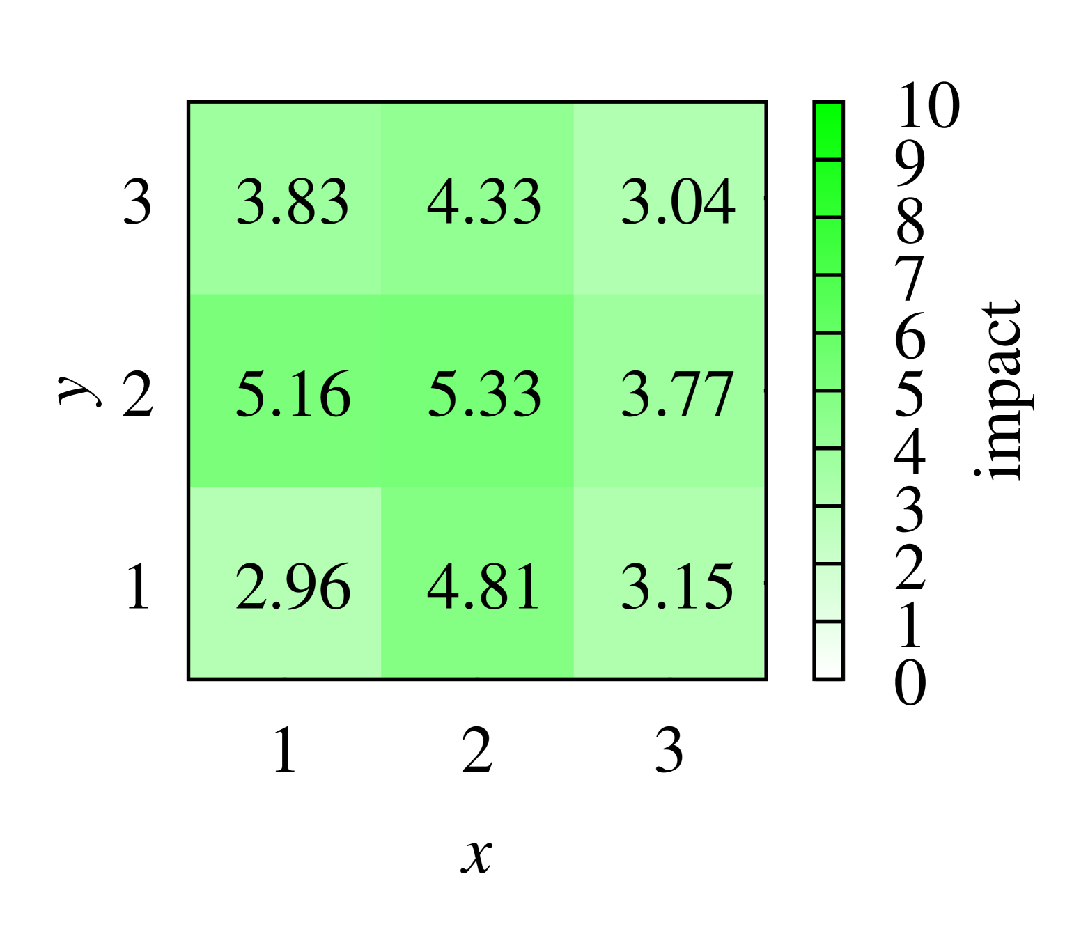
(k) $\mathcal{I}_{(x,y),G}$, $t=2$

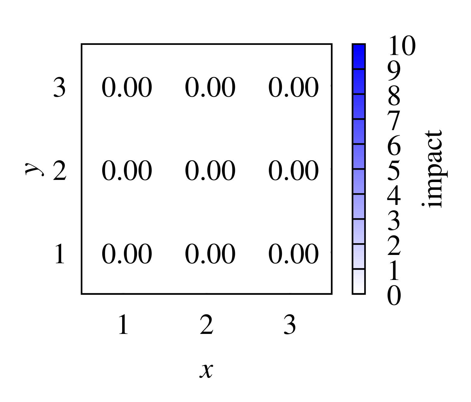
(l) $\mathcal{I}_{(x,y),B}$, $t=2$

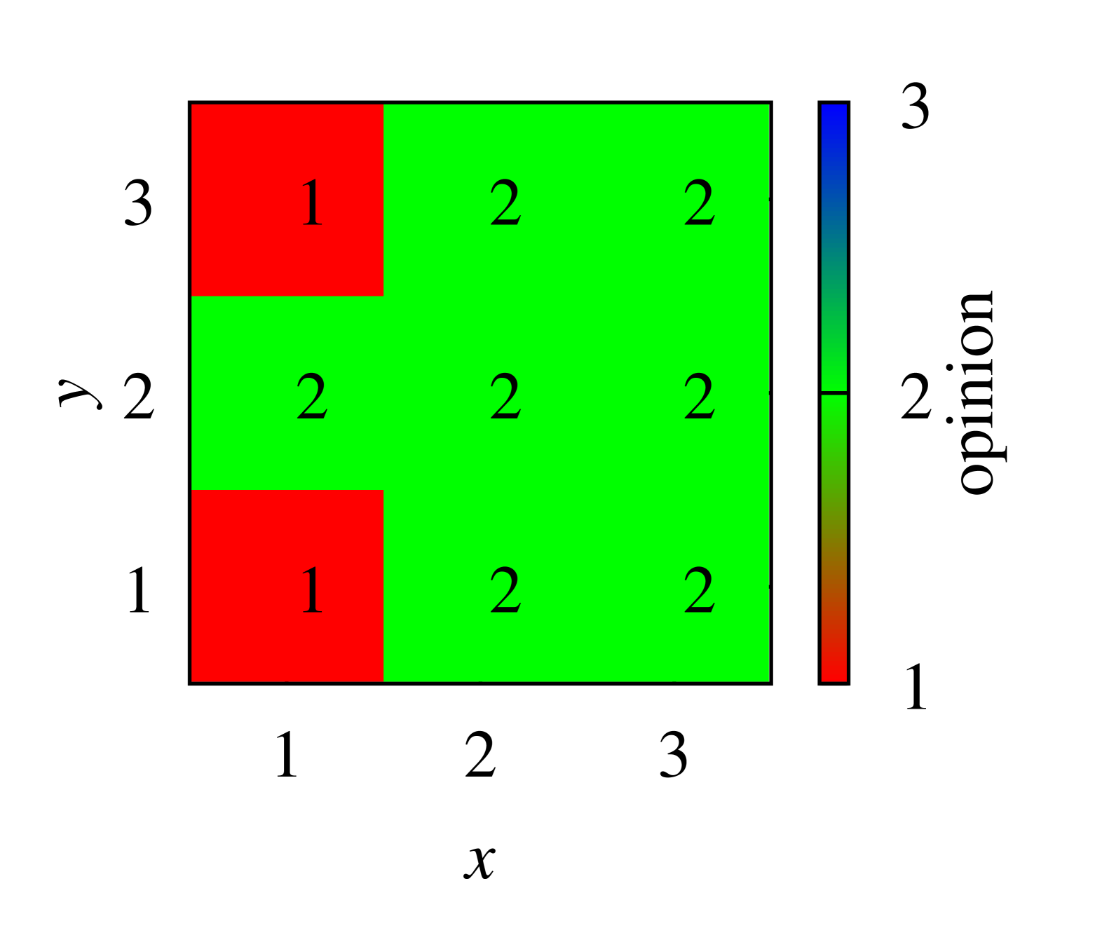
(m) $\lambda_{(x,y)}$, $t=3$

(n) $\mathcal{I}_{(x,y),R}$, $t=3$

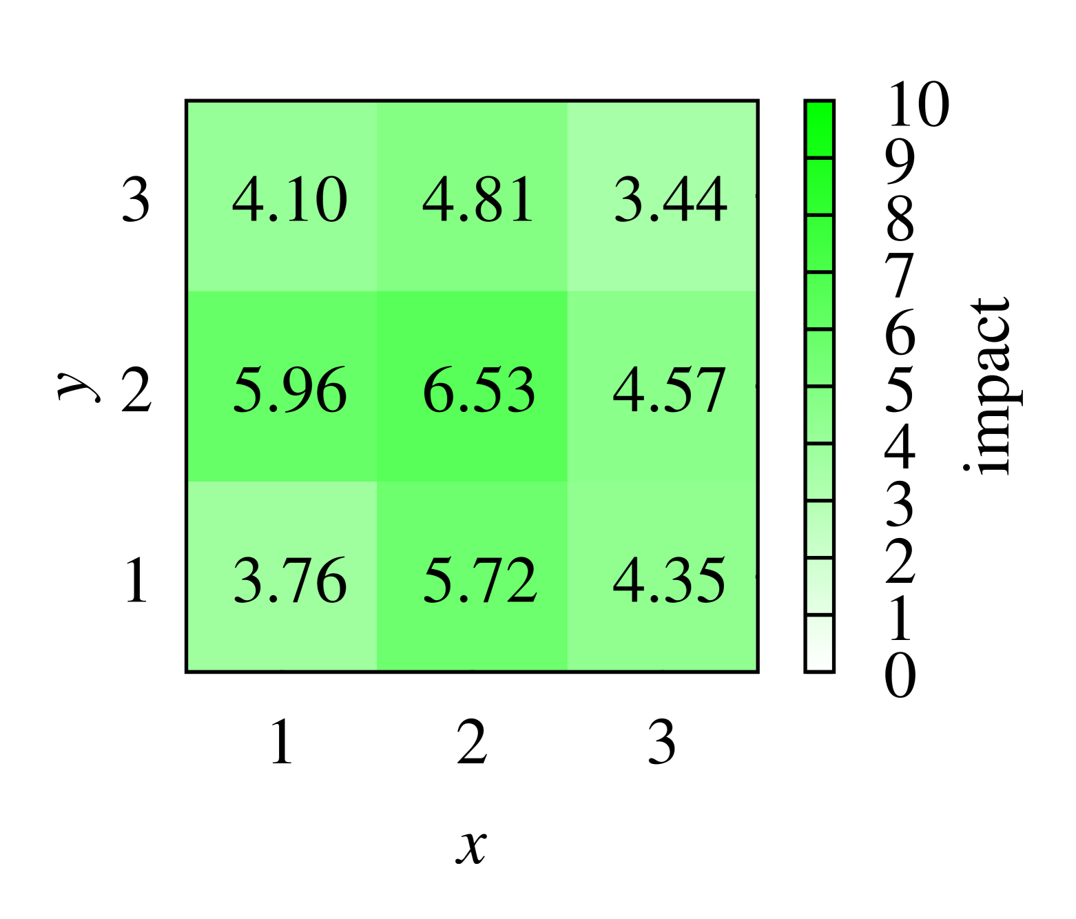
(o) $\mathcal{I}_{(x,y),G}$, $t=3$

(p) $\mathcal{I}_{(x,y),B}$, $t=3$

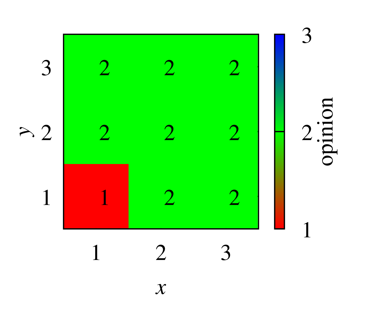
(q) $\lambda_{(x,y)}$, $t=4$

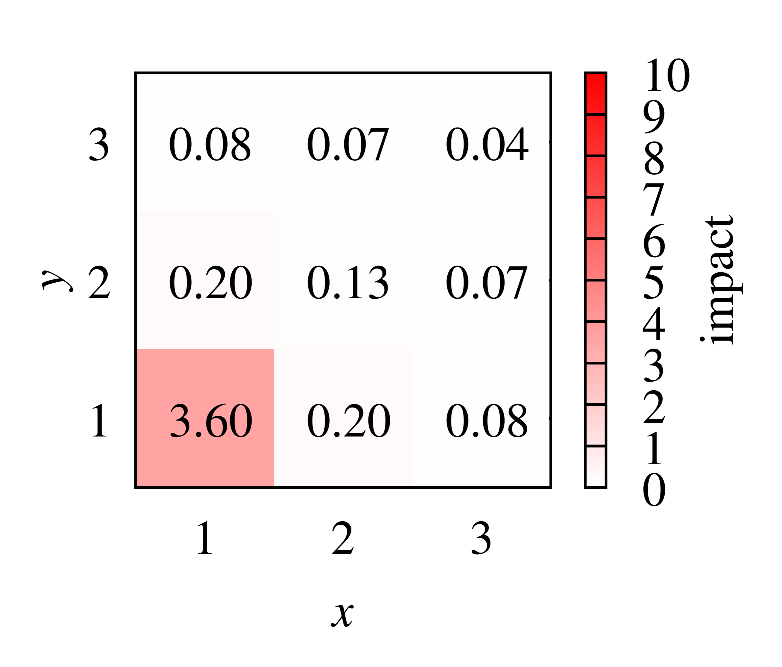
(r) $\mathcal{I}_{(x,y),R}$, $t=4$

(s) $\mathcal{I}_{(x,y),G}$, $t=4$

(t) $\mathcal{I}_{(x,y),B}$, $t=4$

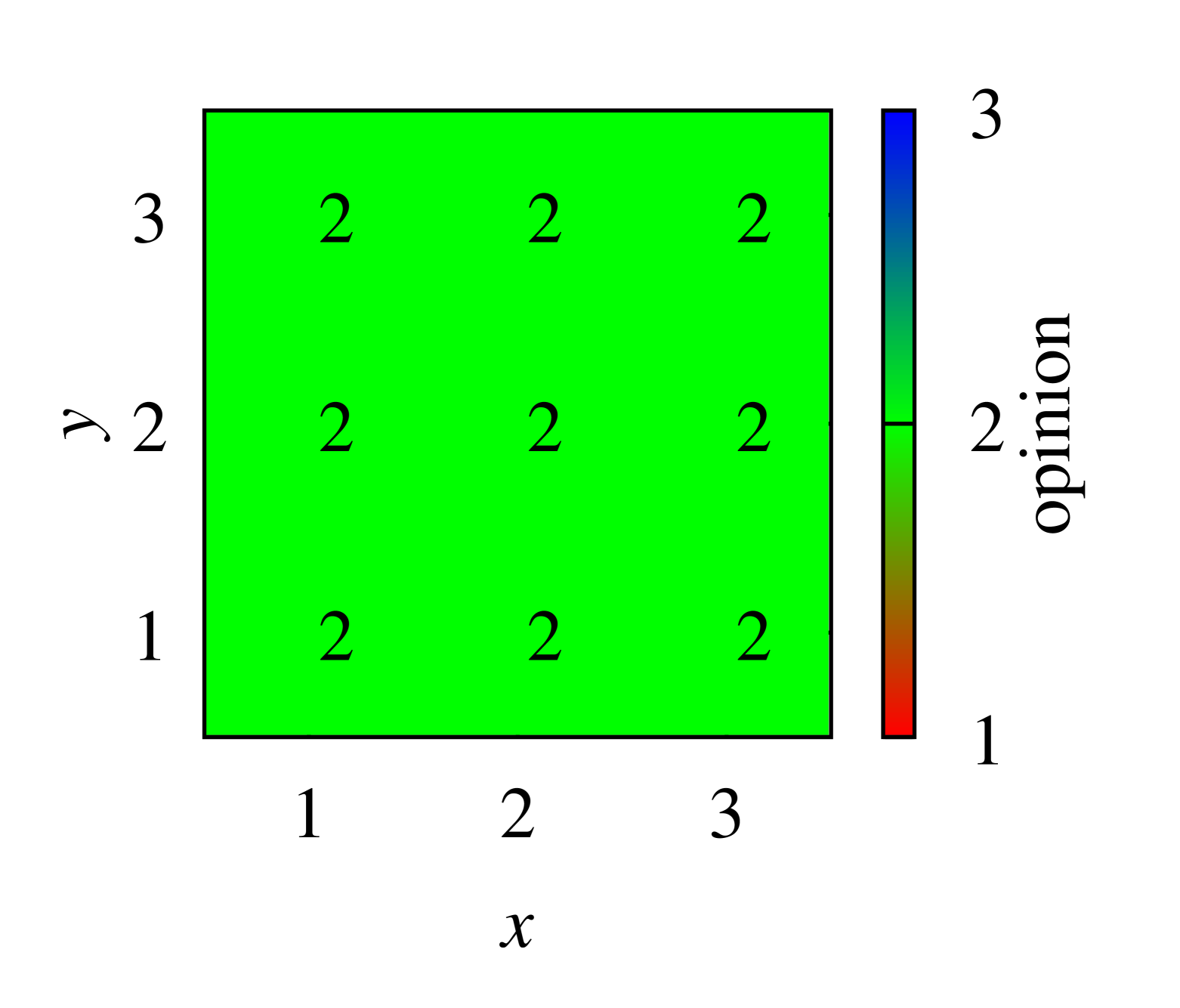
(u) $\lambda_{(x,y)}$, $t=5$

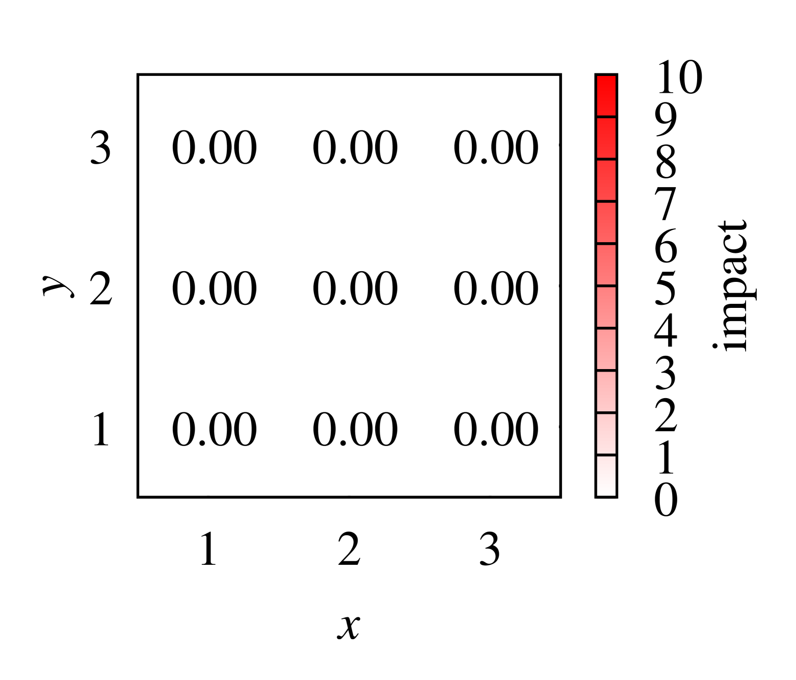
(v) $\mathcal{I}_{(x,y),R}$, $t=5$

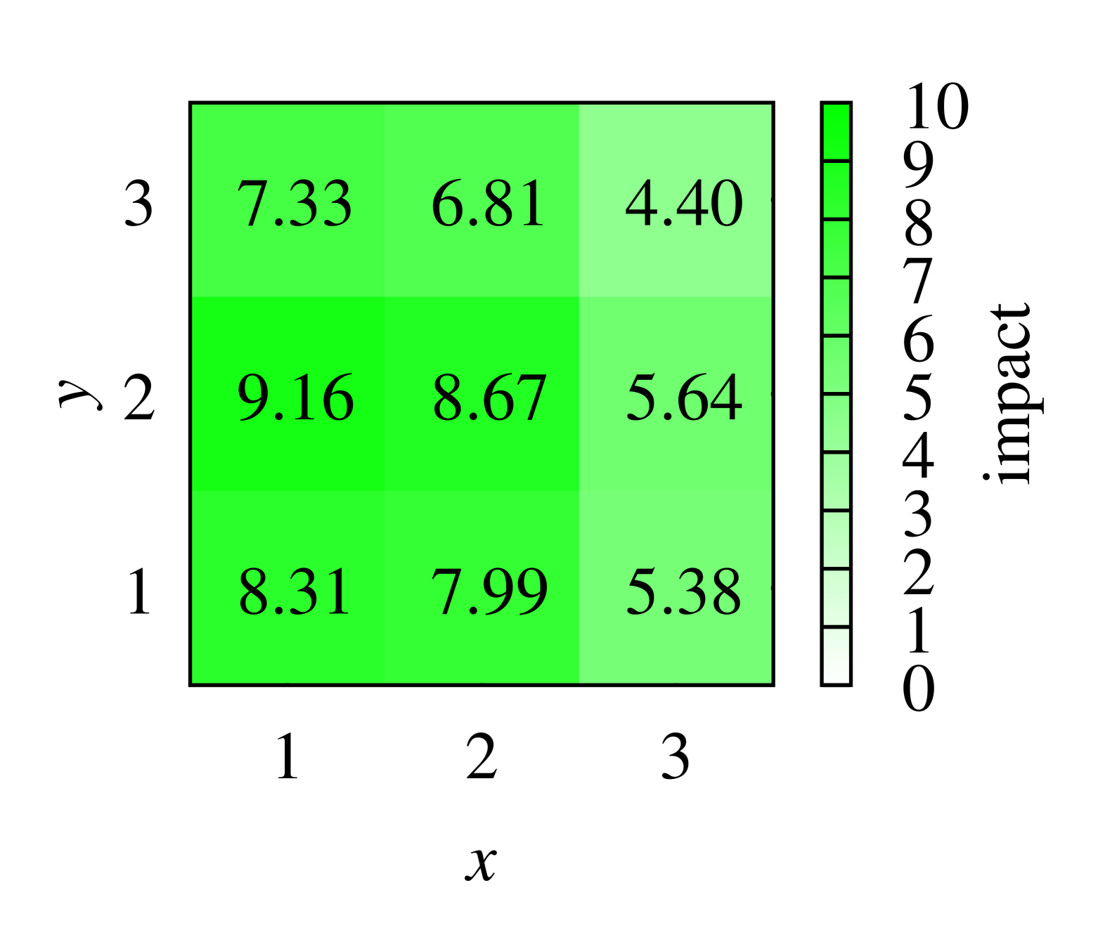
(w) $\mathcal{I}_{(x,y),G}$, $t=5$

(x) $\mathcal{I}_{(x,y),B}$, $t=5$

Figure 8: Example of time evolution of opinions in small system of nine actors. Their opinions $\lambda_{xy}$ are presented in the first column. The second, third, and fourth columns indicate social impacts $\mathcal{I}_{(x,y),C}$ for opinion $C$ equal to ‘red’, ‘green’ and ‘blue’ opinions, respectively

Finally, after completing five time steps, all actors share ‘green’ opinion and the consensus takes place (see Figure˜8(u)). The presence of a sociological equivalent of Muller’s ratchet successfully prevents the restoration of any opinion previously removed from the system. Thus after eliminating the ‘blue’ opinion, it will never have a chance to appear again, and thus we see zeros in matrices Figures˜8(h), 8(l), 8(p), 8(t) and 8(x) and ultimately also on Figure˜8(v)—for impact from eliminated ‘red’ opinions.

Appendix B Distribution of numbers of opinions $n_{\textrm{o}}^{\textrm{u}}$ observed in the system

Figures˜9, 10 and 11 show detailed distribution of $n_{\textrm{o}}^{\textrm{u}}$ on the social temperature $T$ for various parameters $\alpha$ after $t_{\textrm{max}}=10^{3}$, $10^{5}$ and $10^{6}$, respectively.

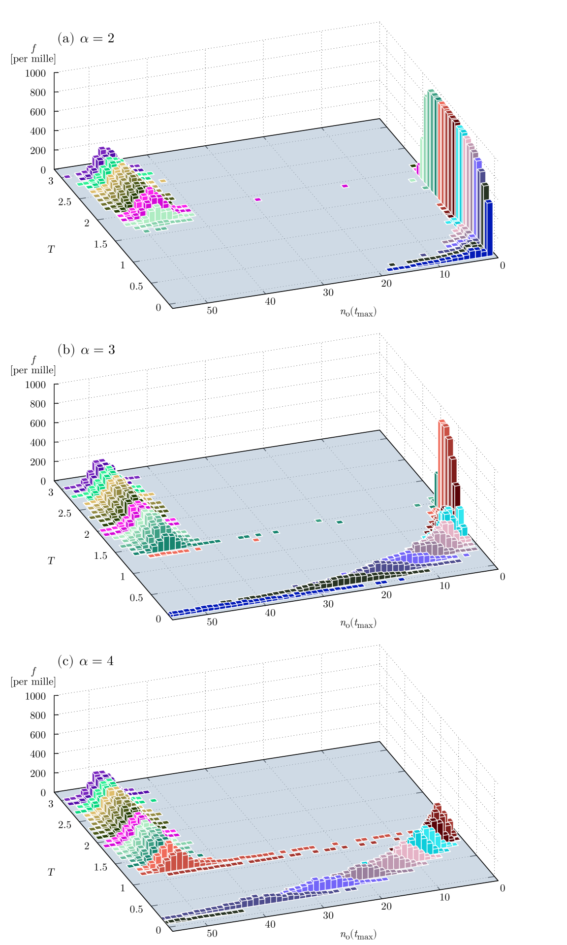
Figure 9: Distribution of $n_{\textrm{o}}(t_{\textrm{max}}=10^{3}$). (a) $\alpha=2$; (b) $\alpha=3$, note: $n_{\textrm{o}}(T=0)\in[16;132]$ (partly visible); (c) $\alpha=4$, note: $n_{\textrm{o}}(T=0)\in[104;232]$ (not visible), $n_{\textrm{o}}(T=0.1)\in[43;115]$ (partly visible)

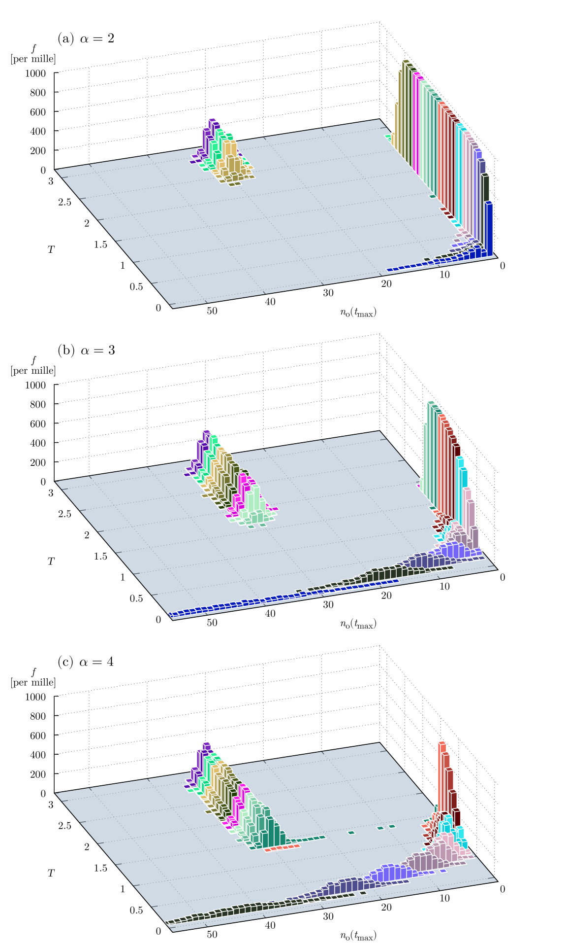
Figure 10: Distribution of $n_{\textrm{o}}(t_{\textrm{max}}=10^{5}$). (a) $\alpha=2$; (b) $\alpha=3$, note: $n_{\textrm{o}}(T=0)\in[17;113]$ (partly visible); (c) $\alpha=4$, note: $n_{\textrm{o}}(T=0)\in[100;244]$ (not visible), $n_{\textrm{o}}(T=0.1)\in[22;70]$ (partly visible)

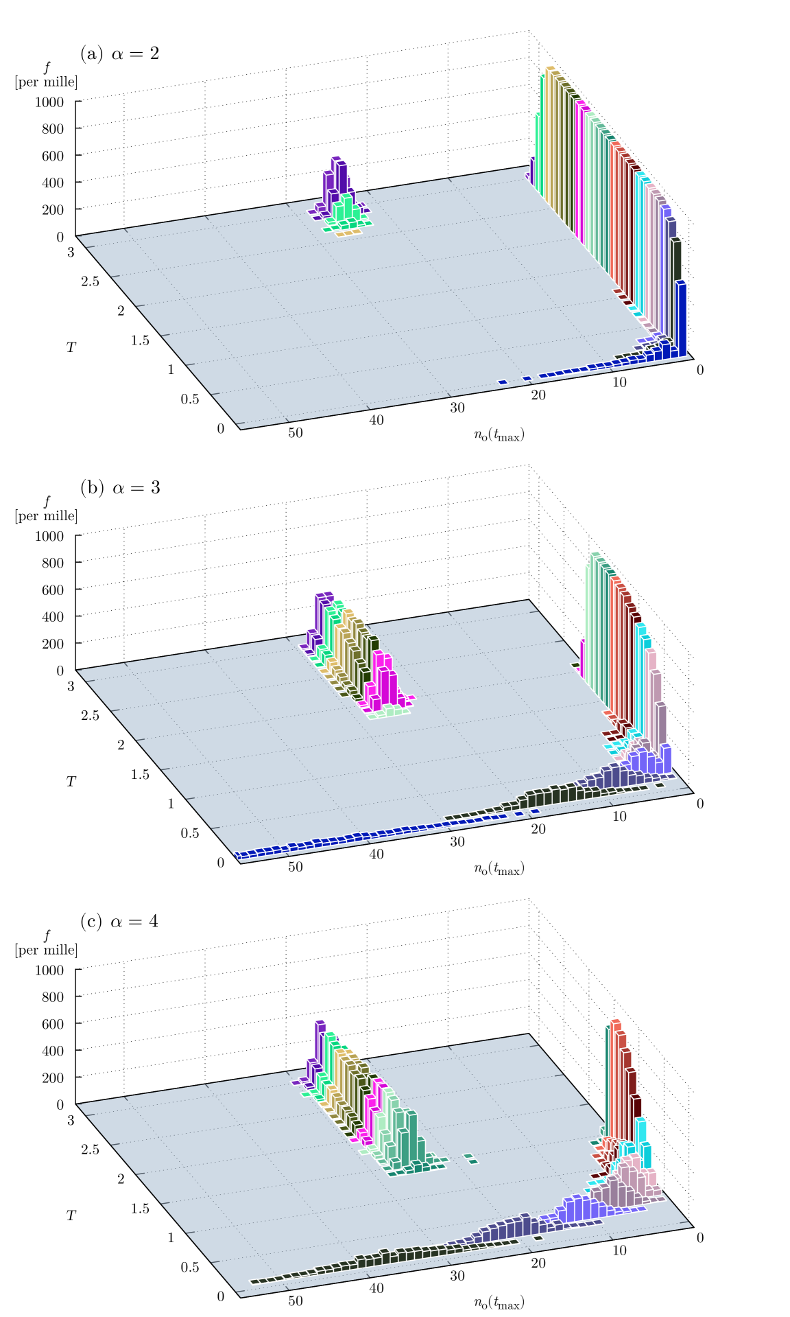
Figure 11: Distribution of $n_{\textrm{o}}(t_{\textrm{max}}=10^{6}$). (a) $\alpha=2$; (b) $\alpha=3$, note: $n_{\textrm{o}}(T=0)\in[19;111]$ (partly visible); (c) $\alpha=4$, note: $n_{\textrm{o}}(T=0)\in[105;241]$ (not visible)

Appendix C Examples of long-time system behavior

In Figure˜12 examples of maps $\lambda$ of opinions frozen in $T=0$ for $\alpha=2$ [Figure˜12(a)], $\alpha=3$ [Figure˜12(b)] and $\alpha=4$ [Figure˜12(c)] are presented.

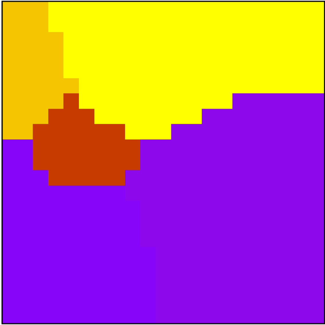
(a)

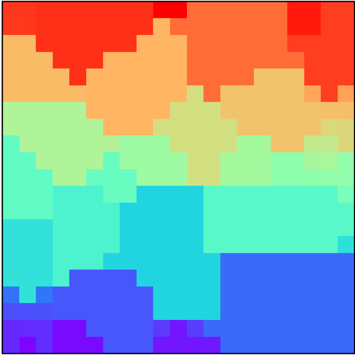
(b)

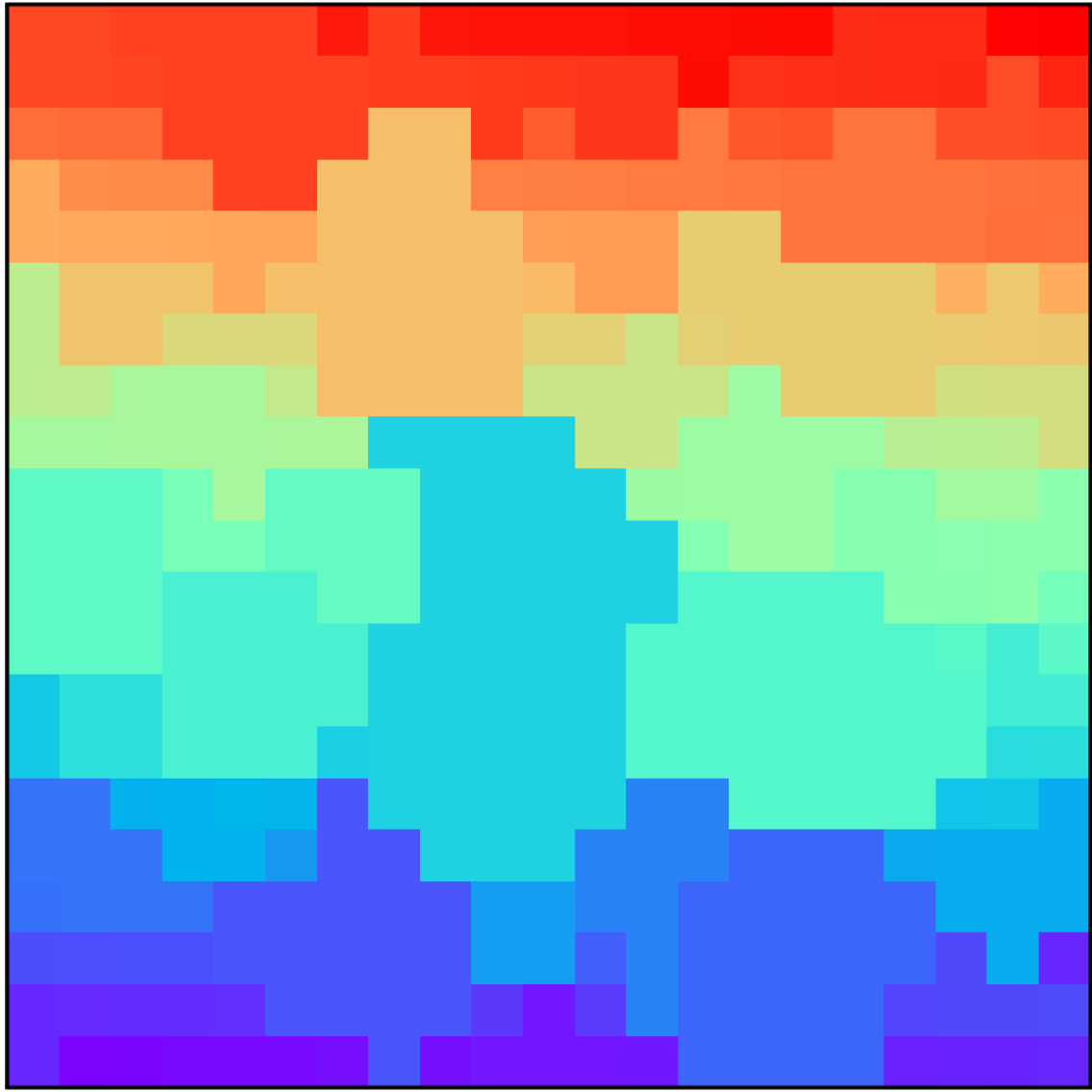
(c)

Figure 12: Examples of maps $\lambda$ frozen at $T=0$ for 12(a) $\alpha=2$, $n_{\textrm{o}}^{\textrm{u}}=4$, 12(b) $\alpha=3$, $n_{\textrm{o}}^{\textrm{u}}=52$ and 12(c) $\alpha=4$, $n_{\textrm{o}}^{\textrm{u}}=146$

In Figure˜13 examples of maps of opinions $\lambda$ [Figures˜13(a), 13(c), 13(e), 13(g), 13(i) and 13(k)] and probabilities of sustaining the opinions $\mathcal{P}$ [Figures˜13(b), 13(d), 13(f), 13(h), 13(j) and 13(l)] after $t_{\textrm{max}}=10^{6}$ for various sets of parameters ($\alpha,T$) are presented.

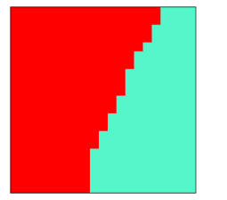
(a)

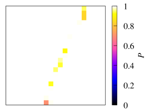
(b)

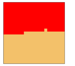
(c)

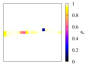
(d)

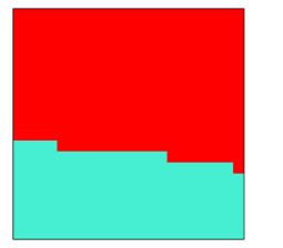
(e)

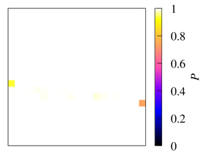
(f)

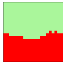
(g)

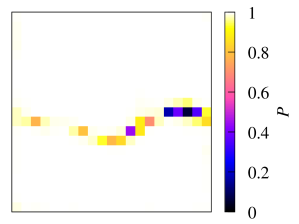
(h)

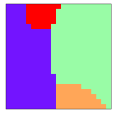
(i)

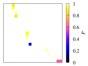
(j)

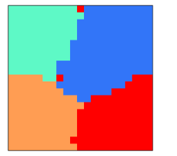
(k)

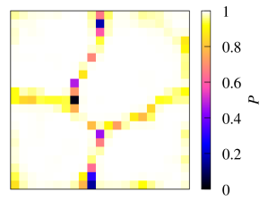
(l)

Figure 13: Examples of maps $\lambda$ and $\mathcal{P}$ after $t_{\textrm{max}}=10^{6}$ for $\alpha=2$, $T=0.5$: 13(a) $\lambda$ 13(b) $\mathcal{P}$; $\alpha=2$, $T=1.1$: 13(c) $\lambda$ 13(d) $\mathcal{P}$; $\alpha=3$, $T=0.5$: 13(e) $\lambda$ 13(f) $\mathcal{P}$; $\alpha=3$, $T=1.1$: 13(g) $\lambda$ 13(h) $\mathcal{P}$; $\alpha=4$, $T=0.5$: 13(i) $\lambda$ 13(j) $\mathcal{P}$; $\alpha=4$, $T=1.1$: 13(k) $\lambda$ 13(l) $\mathcal{P}$;

Appendix D

In LABEL:lst:code the implementation of Latané model rules defined by Equations˜1, 3, 6, 4b and 5 with distance scaling function (2) as Fortran95 code is presented. To compile it with GNU Fortran for multi-threaded execution type
gfortran -fopenmp -O3 latane.f90
in the command line.

Listing 1: Source of Fortran95 code implementing Latané model

⬇

1!!! Latane-Nowak-Szamrej model

!!!

3!!! compile with GNU Fortran with -fopenmp

!!! for multi-threaded execution, e.g.:

5!!! gfortran -O3 -fopenmp latane.f90

7

!!! ###########################################

9module settings

!!! ###########################################

11implicit none

integer, parameter :: seed = 1

13logical, parameter :: randompisi=.true.

integer, parameter :: Xmax=21,Ymax=21,tmax=1e3,L2=(Xmax+1)*(Ymax+1),Run=100,Kmax=Xmax*Ymax

15real*8, parameter :: alpha=2.0d0, T=0.40d0

end module settings

17

!!! ###########################################

19module utils

!!! ###########################################

21use settings

implicit none

23contains

25real*8 function g(x)

real*8 :: x

27 g=1.0d0+x**alpha

end function

29!!! -------------------------------------------

31real*8 function q(x)

real*8 :: x

33 q=x

end function

35!!! -------------------------------------------

37real*8 function d(x1,y1,x2,y2)

integer :: x1,y1,x2,y2

39 d=dsqrt((1.d0*x1-1.d0*x2)**2 + (1.d0*y1-1.d0*y2)**2)

end function

41!!! -------------------------------------------

43end module utils

45!!! ###########################################

program Social_impact

47!!! ###########################################

use settings

49use utils

use omp_lib

51implicit none

integer :: x,y,xx,yy,x1,y1,x2,y2,it,k,irun,no,counter,tau

53real*8 :: r

real*8 :: sump,maxI

55

real*8, dimension (:,:,:,:), allocatable :: gdistance

57integer, dimension (:), allocatable :: histogramno

real*8, dimension (:,:,:), allocatable :: I

59real*8, dimension (:,:,:), allocatable :: prob

integer, dimension (:), allocatable :: ispresent

61integer, dimension (:,:), allocatable :: lambda

real*8, dimension (:,:), allocatable :: p

63real*8, dimension (:,:), allocatable :: s

65allocate( gdistance(Xmax,Ymax,Xmax,Ymax) )

allocate( histogramno(L2) )

67

call srand(seed)

69

histogramno=0

71

!$ write ( *, ’(a,i8)’ ) &

73!$ ’### OpenMP: the number of processors available = ’, omp_get_num_procs ( )

!$ write ( *, ’(a,i8)’ ) &

75!$ ’### OpenMP: the number of threads available = ’, omp_get_max_threads ( )

77if(T.eq.0.0d0) then

print ’(A17)’,"### deterministic"

79else

print ’(A17)’,"### probabilistic"

81endif

83if(randompisi) then

print ’(A18)’,"### random s and p"

85else

print ’(A18)’,"### s_i=p_i=1/2 "

87endif

89print *,’# seed=’,seed

91print ’(A3,7A11)’,’###’,’Xmax’,’Ymax’,’K’,’alpha’,’T’,’tmax’,’Run’

print ’(A3,3I11,2F11.3,2I11)’,’###’,Xmax,Ymax,Kmax,alpha,T,tmax,Run

93print *,’######################################’

95do x1=1,Xmax

do y1=1,Ymax

97do x2=1,Xmax

do y2=1,Ymax

99 gdistance(x1,y1,x2,y2)=g(d(x1,y1,x2,y2))

enddo

101enddo

enddo

103enddo

105!$OMP PARALLEL SHARED(gdistance,histogramno) DEFAULT(PRIVATE)

107allocate( I(Xmax,Ymax,Kmax) )

allocate( prob(Xmax,Ymax,Kmax) )

109allocate( ispresent(Kmax) )

allocate( lambda(0:Xmax,0:Ymax) )

111allocate( p(Xmax,Ymax) )

allocate( s(Xmax,Ymax) )

113

histogramno=0

115

!$OMP DO SCHEDULE(DYNAMIC)

117do 777 irun=1,Run

tau=tmax

119

do x=1,Xmax

121 do y=1,Ymax

if(randompisi) then

123!! random values of s and p

s(x,y)=rand()

125 p(x,y)=rand()

else

127!! homogenous values of s and p

s(x,y)=0.5d0

129 p(x,y)=0.5d0

endif

131 enddo

enddo

133

it=0

135 lambda=0

137 counter=1

do x=1,Xmax

139 do y=1,Ymax

!! random initial opinions

141 ! lambda(x,y)=1+Kmax*rand()

!! every agent has their own opinion

143 lambda(x,y)=counter

counter=counter+1

145 enddo

enddo

147

!! count opinions

149 ispresent=0

do x=1,Xmax

151 do y=1,Ymax

ispresent(lambda(x,y))=1

153 enddo

enddo

155 no=sum(ispresent)

157!! printing system evolution

if(irun.eq.1) then

159 print *,’# irun=’,irun,’it=’,it,’lambda:’

do x=1,Xmax

161 print ’(41I5)’,(lambda(x,y),y=1,Ymax)

enddo

163 print *,"# no=",no

print *,’######################################’

165 endif

167 do 88 it=1,tmax !! starting time evolution

I=0.0d0

169

!! evaluate social impact I(x,y,\lambda) for agent at (x,y) excerted by belivers of \lambda

171 do x=1,Xmax

do y=1,Ymax

173 do xx=1,Xmax

do yy=1,Ymax

175 if(lambda(x,y).eq.lambda(xx,yy)) then

I(x,y,lambda(xx,yy))=I(x,y,lambda(xx,yy))+q(s(xx,yy))/gdistance(x,y,xx,yy)

177 else

I(x,y,lambda(xx,yy))=I(x,y,lambda(xx,yy))+q(p(xx,yy))/gdistance(x,y,xx,yy)

179 endif

enddo

181 enddo

enddo

183 enddo

185 do x=1,Xmax

do y=1,Ymax

187 do k=1,Kmax

I(x,y,k)=4.0d0*I(x,y,k)

189 enddo

enddo

191 enddo

193!! evaluate a probability that agent at (x,y) will take opinion \lambda

do x=1,Xmax

195 do y=1,Ymax

sump=0.0d0

197 do k=1,Kmax

prob(x,y,k)=0.d0 !! new

199 if(I(x,y,k).gt.0.0d0) prob(x,y,k)=dexp(I(x,y,k)/T) !! new if

sump=sump+prob(x,y,k)

201 enddo

do k=1,Kmax

203 prob(x,y,k)=prob(x,y,k)/sump

enddo

205 enddo

enddo

207

!! set (new) opinion of an agent at (x,y)

209 if(T.eq.0.0d0) then !! deterministic case

do x=1,Xmax

211 do y=1,Ymax

maxI=I(x,y,1)

213 lambda(x,y)=1

do k=2,Kmax

215 if(I(x,y,k).gt.maxI) then

maxI=I(x,y,k)

217 lambda(x,y)=k

endif

219 enddo

enddo

221 enddo

else !! probabilistic case

223 do x=1,Xmax

do y=1,Ymax

225 r=rand()

sump=0.0d0

227 do k=1,Kmax

sump=sump+prob(x,y,k)

229 if(r.lt.sump) goto 666

enddo

231666 lambda(x,y)=k

enddo

233 enddo

endif

235

!! count opinions

237 ispresent=0

do x=1,Xmax

239 do y=1,Ymax

ispresent(lambda(x,y))=1

241 enddo

enddo

243 no=sum(ispresent)

if(no.eq.1) goto 22

245

88 enddo !! ending time evolution

247

22 continue

249

!$omp critical(hist)

251histogramno(no)=histogramno(no)+1

!$omp end critical(hist)

253

!! printing system evolution

255 if(irun.eq.1) then

print *,’# irun=’,irun,’it=’,it,’lambda:’

257 do x=1,Xmax

print ’(21I5)’,(lambda(x,y),y=1,Ymax)

259 enddo

print *,"# no=",no

261 print *,’######################################’

endif

263

777 enddo

265!$OMP END DO

267deallocate( I )

deallocate( prob )

269deallocate( ispresent )

deallocate( lambda )

271deallocate( p )

deallocate( s )

273

!$OMP END PARALLEL

275

print ’(A2,A4,4A11)’,"#","K","T","alpha"

277print ’(A2,I4,4F11.3)’,"#",Kmax,T,alpha

279print *, "# histogram of the final number of opinions n_o^u"

do k=1,L2

281 if(histogramno(k).gt.0) print *,k,histogramno(k)

enddo

283

deallocate( gdistance )

285deallocate( histogramno )

287end program Social_impact