Depth Matters: Multimodal RGB-D Perception
for Robust Autonomous Agents

Abstract

Autonomous agents that rely purely on perception to make real-time control decisions require efficient and robust architectures. In this work, we demonstrate that augmenting RGB input with depth information significantly enhances our agents’ ability to predict steering commands compared to using RGB alone. We benchmark lightweight recurrent controllers that leverage the fused RGB-D features for sequential decision-making. To train our models, we collect high-quality data using a small-scale autonomous car controlled by an expert driver via a physical steering wheel, capturing varying levels of steering difficulty. Our models, trained under diverse configurations, were successfully deployed on real hardware. Specifically, our findings reveal that the early fusion of depth data results in a highly robust controller, which remains effective even with frame drops and increased noise levels, without compromising the network’s focus on the task.

I INTRODUCTION

Contemporary approaches to autonomous driving agents use both unimodal and multimodal input for machine learning models in order to provide accurate controls. However, when deploying the agents in the real world, the sim-to-real gap becomes an issue. This is caused by noise affecting sensor readings and computational delays from heavy processing that can significantly impair agent performance.

On the one hand, unimodal RGB input has been successfully used in real-time applications in prior work [1], where a hybrid architecture of convolutional-head with biologically inspired Liquid Time-Constant (LTC) [2] networks was used. They demonstrated exceptional performance in autonomous lane-keeping tasks by directly mapping raw RGB camera inputs to steering commands, outperforming conventional deep networks in both interpretability and resilience to sensor noise. One of the goals is to replicate the model architecture used here as closely as possible, with the necessary adjustments. However, it is known that differential equation (DE) solvers used in their model can cause longer computation times. In recent work, [3] introduced Closed-form Continuous-time Neural Network (CfC), a variant of the ODE-based continuous LTC network. Another efficient extension is by introducing a liquid capacitance term into the model [4] on top of saturation [5], called Liquid Resistance Liquid Capacitance Network (LRC). These solutions can be beneficial in more lightweight hardware setups, ensuring faster reaction times, which we implement and test in this paper.

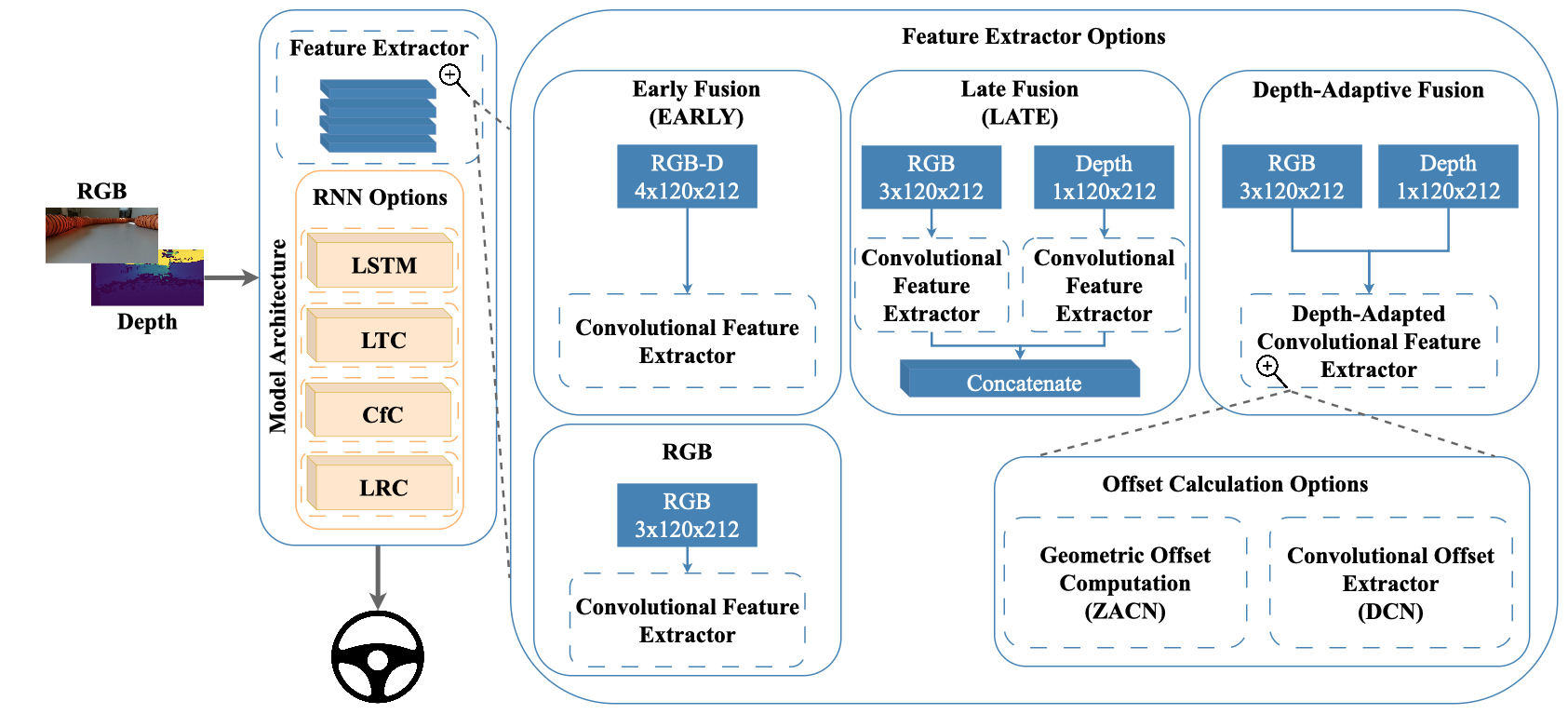
Figure 1: High-level overview of the model architectures deployed on our hardware, following a channels-first configuration

On the other hand, unimodal approaches face inherent limitations in complex real-world scenarios where depth perception is critical for obstacle avoidance and path planning. To tackle this challenge, we employ multimodal sensory fusion. RGB-D input is used in simulation both in [6] and  [7]. Although these approaches demonstrate success in simulated environments, their applicability to real-world scenarios remains unexplored, especially on small-scale platforms like roboracer [8]. This paper seeks to bridge that gap through its real-world application.

In addition, the fusion of RGB-D information has been widely researched in computer vision, mainly using Convolutional Neural Networks (CNN)[9]. A widely used approach is introducing depth information as a new channel to the input of 2D convolutions, which yields the best results in [7]. Alternatively, the authors of [10] use depth information in the computation of Deformable CNNs [11, 12], which aim to enhance spatial flexibility. Their approach leads to more accurate object classification than with RGB alone. We aim to test these more advanced approaches not in computer vision but in a control task.

This paper aims to investigate the integration of RGB-D data for autonomous driving in a lightweight real-world scenario. In this way, we can achieve optimized multimodal models for the small-scale autonomous system roboracer with fast reaction times and behavior comparable to that of an experienced human driver.

In summary, our contributions in this paper are as follows:

• We show that depth information is crucial, RGB alone is not enough for robust navigation.

• A systematic comparison of RGB-D fusion architectures for autonomous driving, evaluating depth-as-channel (early fusion and late fusion) and depth-aware deformable CNNs (DCN [11] and ZACN[13]) to optimize feature extraction for robust perception in noisy real-world environments.

• Lightweight recurrent controller benchmarking for real-time efficiency, which uses the extracted features from our multimodal vision block from the previous point for control.

• Bridging the sim-to-real gap for RGB-D multimodal models with recurrent controllers: the first deployment of a depth-enhanced network on a physical roboracer vehicle, achieving a smooth and noise-robust controller.

The rest of the paper is organized as follows. Section II reviews prior work on multimodal perception and autonomous driving architectures. In Section III, we describe our hardware configuration and dataset collection process. Section IV summarizes our proposed model architectures integrating RGB-D fusion. In Section V, we evaluate the impact of depth-aware feature extraction via vision fusion heads paired with recurrent controllers for sequential steering prediction. Finally, we discuss our results in Section VI.

II RELATED WORK

In this section, we review recent studies in autonomous steering control using deep-learning methods, focusing on RGB-based approaches, depth modality fusion, as well as state-of-the-art methods for the roboracer platform. We highlight key advancements, limitations in real-world deployment and the gap in efficient resource-constrained solutions.

II-A Unimodal RGB Input

A critical achievement in the context of end-to-end autonomous driving is [14], in which a 9-layer Convolutional Neural Network (CNN) trained on RGB input successfully predicted steering commands on a drive-by-wire vehicle. Although it is shown the model learned useful road features, it remained impossible to assess which segments of the network contributed to its decisions due to the large scale of the network.

Alternatively, [15] tackled the limitations of traditional CNN-based steering models by introducing a temporal dependency-aware approach. They propose a C-LSTM network architecture with CNN for feature extraction, followed by Long Short-Term Memory (LSTM) [16]. After training with RGB images obtained from a simulated environment, the evaluation of the model revealed effective feature extraction and autonomy in mostly obstacle-free scenarios. However, real-world deployment remained untested.

Addressing the issues of interpretability and real-time use that such traditional deep learning methods pose, the authors of [1] introduced a compact bio-inspired neural controller, called Neural Circuit Policy (NCP). Their model significantly out-performed purely CNN methods both in simulation and hardware deployment, using RGB data.

Another study incorporates optical flow extracted from RGB frames to improve steering estimation [17]. Their approach integrates CNN-based feature extraction with Recurrent Neural Network (RNN)’s, including LSTM and NCP. By employing both early and hybrid fusion techniques, they demonstrated that incorporating optical flow significantly reduces steering estimation error compared to RGB-only methods in dataset-only evaluation. Nevertheless, the results are limited to dataset experiments, without on-board evaluation.

II-B Multimodal Input

Even though several studies have explored different approaches to improve the performance of autonomous driving models by leveraging RGB-D information, many of them lack real-world testing to confirm practical viability.

Notably, [6] presents a Recurrent CNN (RCNN) trained by fusing camera and LiDAR data. Their results accentuate the importance of multimodal perception for enhancing autonomy, outperforming RGB-only models. However, despite its strong performance in simulation, the model was not evaluated in a real-world driving scenario, leaving its practical deployment untested.

Similarly, another study investigates the impact of multimodal perception on fully autonomous driving, particularly focusing on early, mid, and late fusion techniques [7]. Using the CARLA simulator, the authors compare the performance of single-modality (RGB/depth) and multimodality. Their results indicate that early fusion multimodality significantly outperforms single-modality models, especially under challenging driving conditions. However, real-world validation was not performed, limiting its practical insights.

II-C State-of-the-Art of roboracer

End-to-end (E2E) deep learning approaches have been widely explored for autonomous racing on the roboracer platform, with multiple works leveraging Deep Reinforcement Learning (DRL) for control [18, 19, 20]. In contrast, supervised learning-based approaches for roboracer are relatively unexplored, with TinyLidarNet [21] being a key recent contribution. TinyLidarNet introduces a lightweight LiDAR-based CNN model, which maintains fast inference efficiency on low-end microcontrollers. However, its reliance on LiDAR raises concerns about robustness in challenging environments. As a separate study [22] has shown, LiDAR performance drops to 33% while depth cameras maintain full-ranging capabilities in adverse conditions. Given these findings, our work diverges from TinyLidarNet by adopting an RGB-D-based supervised learning approach, aiming to benefit from stereoscopic camera sensing’s robustness and resilience to lighting variations.

Collectively, these studies highlight the shift in autonomous systems toward multimodal learning and compact neural controllers, yet real-world deployment remains limited. Our goal is to enable autonomous agents to navigate their environment reliably on low-cost, resource-constrained hardware. By deploying efficient RGB-D-based models, we ensure practicality and robustness in real-world scenarios.

III METHODS

In this section, we present the methodology used to develop and evaluate our model architectures. We start by describing the hardware setup and our data collection process, followed by outlining the dataset creation pipeline, including the measures implemented to ensure high-quality training data.

III-A Hardware Setup and Data Collection

The platform we used in this paper is a one-tenth-scaled car, referred to as roboracer in the autonomous driving research community. Further details about the roboracer platform, including in-depth hardware description and state-of-the-art applications are detailed by the platform creators in [23].

The major hardware components of the roboracer platform include a lower-level chassis, an upper-level chassis, and several autonomy elements. The embedded computing platform is a 13th Gen Intel(R) Core(TM) i7-1360P. Most importantly for optical vision, we integrated a stereoscopic depth camera (Intel RealSense D435i) into the hardware stack. According to the datasheet, key application-specific properties of the camera include a range of 10m (best performance between 0.3m and 3m), and 69$\degree$$\times$42$\degree$ RGB FOV, 87$\degree$$\times$58$\degree$ Depth FOV.

Given the 30fps limitation of the RGB camera, the same number of fps was used for the depth stream. Furthermore, both camera streams were configured to 848$\times$480px resolution, which is the optimal recommended resolution for the depth camera.

We set up the driving area indoors, using standard roboracer pipes to build different track configurations. Our choice was motivated by the pipes typically used during competitions, which provide an excellent application for using a multimodal optical stream to control the steering.

We built a series of 5 tracks to offer a variation of successive turns, either of different curvatures or lengths before, during, and after each turn, as seen in Figure 2. In order to increase the dataset size, all tracks were driven both clockwise and anti-clockwise.

A driver with 10 years of frequent driving experience was chosen to control the car on different tracks. The driver was given control of the vehicle through a racing steering wheel and pedals, with a speed cap of 0.9 m/s. We introduced the speed cap after several trials were made by the human driver around track Figure 2(a) without any speed restrictions. We found that due to the narrow FOV of the camera, the driver was most comfortable driving with a maximum speed of 0.9m/s.

The data flow of the driving stack during data collection is illustrated in Figure 3. In order to simulate a first-person point of view, we redirected the RGB stream from the onboard camera via the network to a second device with a monitor placed in front of the driver. While driving, rosbags were being recorded on all available car topics, excluding the RGB topic. The RGB data stream was saved as videos while driving on the support device connected to the monitor.

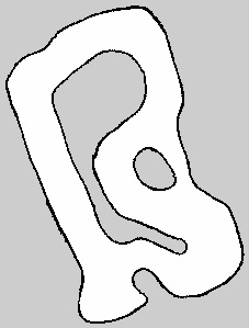
(a)

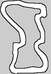
(b)

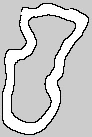
(c)

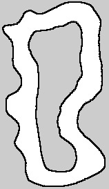
(d)

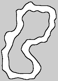
(e)

Figure 2: Tracks built for human expert data collection.

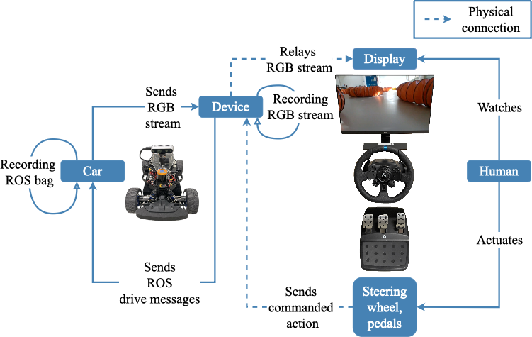
Figure 3: Overview of our driving stack used during the data collection step.

The driver was allowed a few trial runs on each track before the data recording was started in order to get accustomed to the camera’s field of view and the difficulty of the track. For Figure 2(a), we instructed the driver to take the longer route at the intersection.

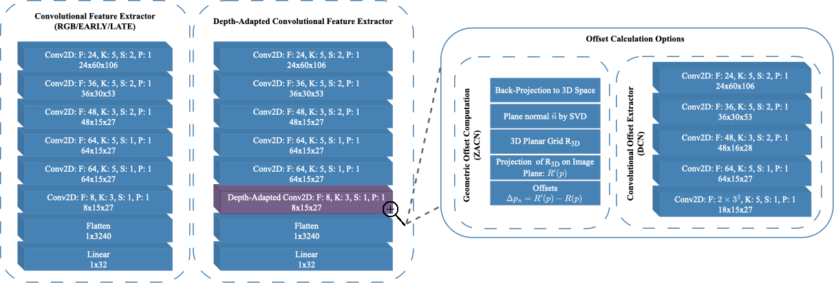
Figure 4: The sequence of layers in the convolutional heads is as follows. The Convolutional Feature Extractor is used with an RGB input of size 3×120×212. In the early fusion (EARLY) method, it processes an input of size 4×120×212. In the late fusion (LATE) method, it is used twice, treating RGB and depth as two separate input streams of sizes 3×120×212 and 1×120×212, respectively, and concatenating their features after the last layer. The Depth-Adapted Convolutional Feature Extractor has two versions: (1) the DCN, which includes a Convolutional Offset Extractor, and (2) the ZACN [13], which incorporates Geometric Offset Computation. In the hyperparameters section: F denotes the number of filters, K the kernel size, S the stride, and P the padding.

III-B Dataset Collected for Open-Loop Training

To synchronize the rosbags and RGB frames, we leveraged the mutual 30fps rate chosen to configure the camera.

Firstly, the messages on the depth topic were extracted from each rosbag [24]. Their content consists of uint16 1-channel images representing the measured distance for each pixel. We parsed each frame to RGB by creating a colormap on the pixels based on their distance with respect to the maximum measured value. Then, we generated depth videos from each rosbag and stamped every frame with its corresponding number.

As a second step, we manually synchronized the original videos with the depth. The original videos were also broken down and stamped by frame number as a preparatory procedure. Before the start of each recording session, we presented visual cues to the camera to synchronize the streams. In this way, we were able to log the frame number corresponding to each visual cue for both the RGB and depth streams. Furthermore, we logged frame numbers corresponding to the start and end of every lap in all recordings.

Thirdly, the resolution of the streams was downscaled to 1/4th of the initial scale. For this purpose, we tested several rescaling algorithms: nearest neighbor, Gaussian, Lanczos [25], and Catmull-Rom [26]. As expected, nearest neighbor downsampling produced grainier results, while Gaussian downsampling blurred the stream. As neither was desirable, Lanczos-3 was chosen over Catmull-Rom for producing overall sharper results.

Lastly, the depth topic messages were iterated over based on the lap frame intervals in each recording. This led to obtaining the timestamp of each frame message, which we then used to find the corresponding steering commands as in [24] by interpolating the values between two timestamps. In this way, each RGB frame and depth message was labeled with the commanded steering angle and saved as .npz files. Through this approach, we obtained a dataset of approximately $100\,000$ labeled frames from all collected data.

III-C Work Environment

The machine used for training the models runs Ubuntu 20.04.6 and has $3\,072$ CUDA cores and 12 GB of GDDR5 memory. Due to its out-of-the-box interoperability and wide range of packages in the area of computer vision, we chose PyTorch as a framework, and configured a Conda virtual environment. Code is available in our GitHub repository.

IV EXPERIMENTAL SETUP

In total, 20 model architectures were designed and implemented. We focused on one unimodal and 4 multimodal approaches for feature extraction.

IV-A Unimodal RGB Setup

The implemented unimodal architecture closely follows [1], with a convolutional head illustrated in Figure 4 consisting of 6 convolutional layers which feed their final output to the RNN of choice. This approach aims to extract relevant features of the RGB input and use them as input to RNN s, which make memory-based steering commands. We refer to this method as RGB in the next sections.

IV-B Multimodal RGB-D Setups

(i) The first multimodal approach is an early fusion approach (referred to as EARLY), introducing the depth values as a fourth channel to the RGB input of the previously described convolutional head. This type of method for CNN’s achieved the best results in [6] and [7]. This architecture is shown in Figure 4 as the Convolutional Feature Extractor.

(ii) Similarly to [27], the second multimodal architectural method is a late fusion method (referred to as LATE). This essentially presents a two-stream architecture, where different CNN’s are used for each of the inputs.

(iii) The final chosen approach illustrated in Figure 4 as Depth-Adapted Convolutional Feature Extractor, is processing the multimodal input using Deformable CNN. As the goal of deformable convolutions is to hone spatial adaptation of kernels, we only use the operation once, in the last layer. In this way, we ensure that the most relevant features extracted from RGB using standard convolution are simply enhanced by offsets that are extracted from depth information. To this end, two techniques were utilized for calculating the convolutional offsets for the deformable layer.

(iii-a) The first technique in this subcategory relies on extracting the offsets from the single-channel depth data using CNN. We refer to this as DCN.

(iii-b) The second technique, which we refer to as ZACN, is based on [13]. The intrinsic camera parameters used by this method were obtained from the device used during data collection.

IV-C Recurrent Models

The feature extractor models are further differentiated from each other based on 4 RNN backbone choices: LSTM, LTC, CfC and LRC.

The LTC and CfC backbones use a NCP of 19 neurons, i.e., 12 inter-neurons, 6 command neurons, and 1 motor neuron, as LTCs were configured in [1]. We adapted CfCs to this setup as they are the closed-form solutions of LTCs. The LSTM and LRC architectures are configured to have a standard size of 64 features in the hidden state. All RNN’s use a sequence length of 16 frames.

IV-D Training and Metrics

Regarding the dataset, the order of the 10 recordings (2 directions for each track) was shuffled. Starting from this randomized order, we split the dataset into a 60/20/20 ratio representing training, validation, and test data. The split datasets are further shuffled before being fed to the models.

All run configurations include modifiable arguments for the RNN model, input mode, the type of per-channel normalization in the normalization layer, padding, and learning rates. We experimented with Min-Max normalization, Z-Score normalization, and Min-Max followed by Z-Score. During training, we set the maximum epoch number to 100 epochs with a batch size of 20, constrained by the available computational resources. To prevent overfitting, training stops early if the validation loss does not improve for three consecutive epochs. We used Tensorboard to log and analyze all models’ training, validation, and testing results.

We used the Adam optimization algorithm  [28] with learning rates of $\{10^{-3},10^{-4},10^{-5}\}$ and $\epsilon=10^{-7}$ for numerical stability. To predict continuous steering commands from multi-dimensional input, we used the Mean Squared Error (MSE) as loss function. Since MSE produces strictly positive values, losses closest to 0 indicate the most accurate estimations.

V RESULTS

In this section, we summarize our findings on the various model architectures presented in Section IV. First, we describe the results from the passive test using the collected dataset, followed by the deployment results of the best models.

V-A Open-loop Results

We follow the training procedure described in Section IV-D. Since we use supervised learning at each timestep, the next input frame is not influenced by the model’s previous decision, which is known as an open-loop setting.

Table I presents our best open-loop test loss results using the recorded dataset. We found that for each feature extractor, the two best-performing models are LSTM and LRC, except for RGB, where CfC performed better than LRC.

TABLE I: Test results, averaged over 3 seeds. Models were trained, validated, and tested on the collected dataset. Loss values are scaled by $\times 10^{-3}$. The two best-performing recurrent models for each feature extractor are highlighted.

	LSTM	LTC	CfC	LRC
EARLY	$\mathbf{7.53\pm 0.49}$	$11.73\pm 3.82$	$12.60\pm 4.42$	$\mathbf{8.23\pm 1.71}$
LATE	$\mathbf{5.93\pm 0.77}$	$9.93\pm 1.02$	$8.97\pm 1.63$	$\mathbf{7.80\pm 0.92}$
ZACN	$\mathbf{8.27\pm 1.22}$	$10.27\pm 0.90$	$9.53\pm 1.17$	$\mathbf{8.07\pm 1.10}$
DCN	$\mathbf{8.77\pm 1.63}$	$22.50\pm 9.75$	$11.65\pm 1.85$	$\mathbf{9.37\pm 1.88}$
RGB	$\mathbf{9.57\pm 2.37}$	$13.30\pm 1.91$	$\mathbf{11.87\pm 1.74}$	$12.00\pm 2.14$

V-B Closed-loop Results

After training and evaluating the models on the passive dataset, we were interested in how they would adapt to a closed-loop setting when deployed on hardware. Since we had a total of 20 models (5 feature extractors × 4 RNN options), we chose to test only the most promising ones that demonstrated good performance on the dataset.

To ensure a balanced evaluation of both the feature extractors and the RNNs, we created test groups based on both components. Specifically, we selected the best two recurrent models for each feature extractor and the best two feature extractors for each recurrent model across all seeds. The results are presented in Table II.

TABLE II: The summary of the closed-loop testing is presented, with results grouped by different feature extractors on the left and by recurrent models on the right. For each feature extractor, we deployed the two best-performing RNN options. Similarly, for each RNN, we deployed the two best-performing feature extractor options based on the test results from the recorded passive dataset. S denotes success of 5 consecutive laps on the test track.

Feat.-Extr.	RNN	S
EARLY	LSTM	✓
	LRC	✗
LATE	LSTM	✗
	LRC	✗
ZACN	LRC	✓
	LSTM	✗
DCN	LSTM	✓
	LRC	✗
RGB	LSTM	✗
	LRC	✗

RNN	Feat.-Extr.	S
LSTM	LATE	✗
	EARLY	✓
LTC	LATE	✗
	ZACN	✗
CfC	LATE	✓
	ZACN	✓
LRC	LATE	✗
	ZACN	✓

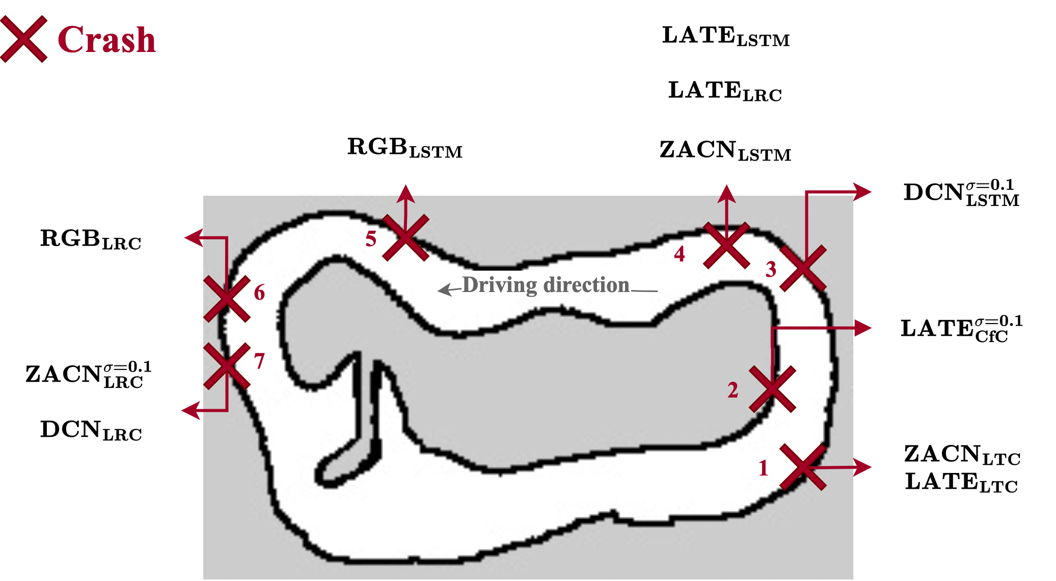
Figure 5: Extraction of the map used during closed-loop active testing. Problematic turns are marked with an ’X’ to indicate crashes. Labels specify which model crashed at each point.

We found that this closed-loop setup is very challenging for many of the trained models, with only a subset successfully completing 5 continuous laps without crashing. We marked the sections in Figure 5 where crashes occurred. Interestingly, the LATE feature extractor only succeeded with the CfC model, even though it was not among the two best recurrent models for the LATE type in the passive open-loop test (as shown in Table I). However, we evaluated it because CfCs demonstrated the best performance with this feature extractor method, which highlights the effectiveness of our double grouping approach for feature extractors and recurrent models, respectively. This also illustrates the sim-to-real gap, highlighting the performance mismatch between the open-loop setup and real hardware deployment.

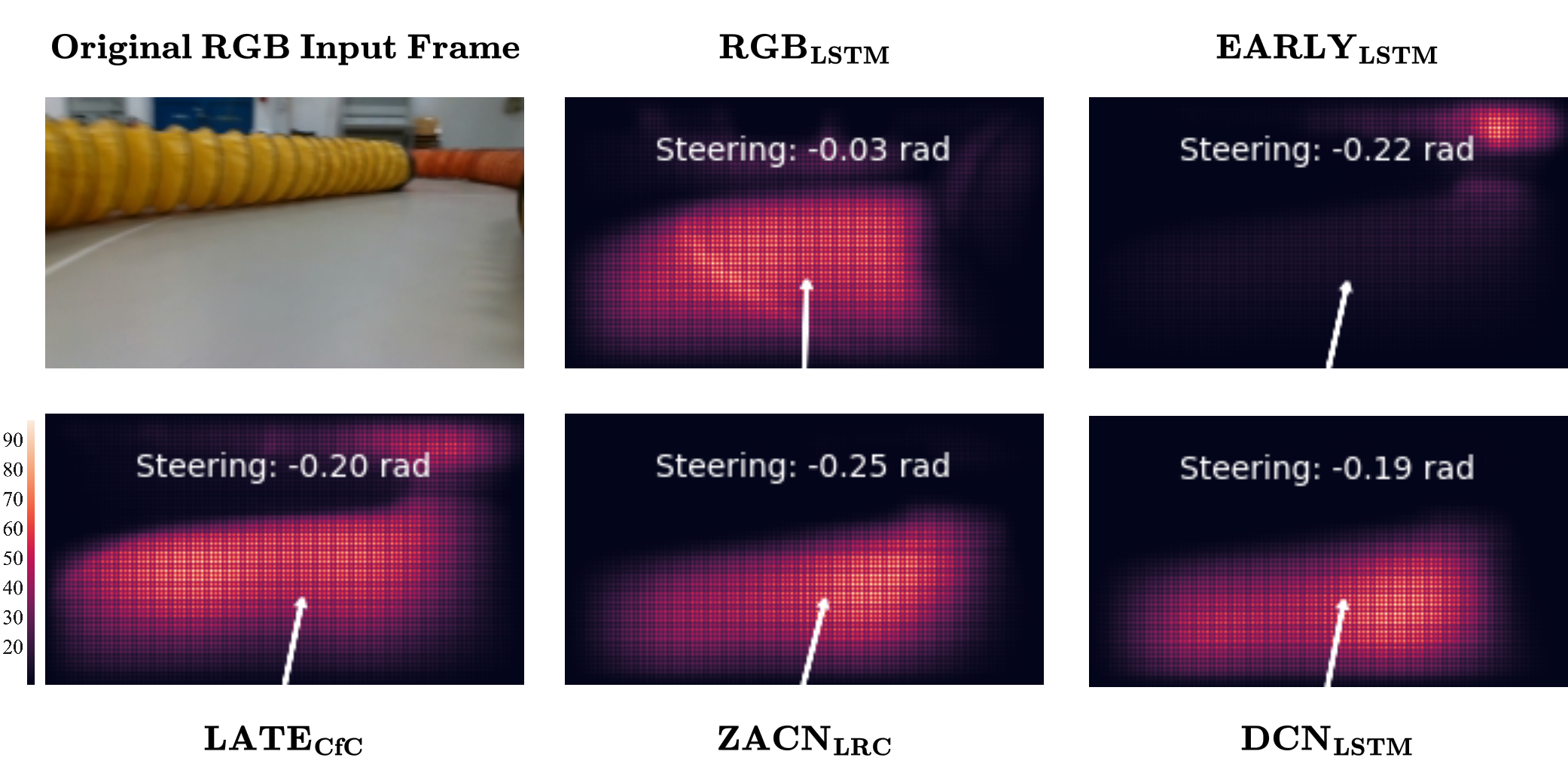
Figure 6: Attention maps during closed-loop testing, evaluated on RGB_LSTM, and the models that achieved full autonomy for 5 consecutive laps. The chosen frame is prior to the RGB_LSTM model crash at landmark 5 of Figure 5.

We explored the underlying attention mechanism of these models to gain insight into which parts of the input they focus on the most. To calculate this, we used the VisualBackProp method [29], where bright regions indicate where the model focused its attention. The attention maps are displayed in Figure 6. We found that the EARLY_LSTM maintains its focus on the more distant regions, while the other models focus more on the road directly ahead. The attention of the LATE_CfC, ZACN_LRC, and DCN_LSTM models tends to explore the right side of the road more, while the RGB_LSTM model keeps its attention more evenly in front, without focusing on the turn. We hypothesize that this lack of focus on the turn contributed to the RGB_LSTM’s crash.

V-C How Robust Are the Deployed Models?

We selected models that completed 5 consecutive laps on the track without crashing for further evaluation under noisy conditions. These models include EARLY_LSTM, LATE_CfC, ZACN_LRC, and DCN_LSTM. To test their robustness, we added additional Gaussian noise with a mean of 0 and a variance of 0.1 to the input stream. Only the EARLY_LSTM model handled successfully this challenging condition, while the others failed, resulting in crashes at Points 2, 7, and 3, as shown in Figure 5, respectively.

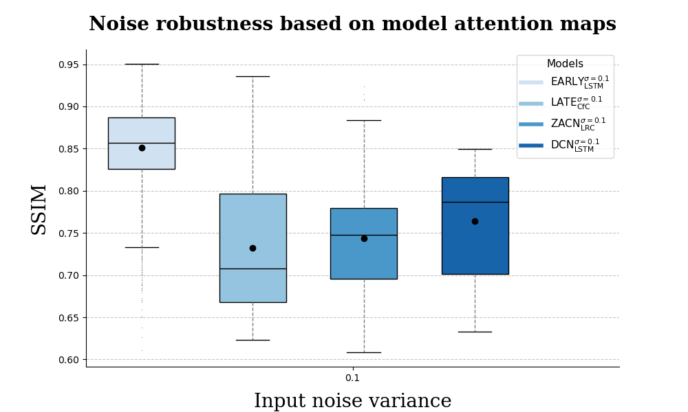
Figure 7: The Structural Similarity Index (SSIM) values for the EARLY_LSTM, LATE_CfC, ZACN_LRC, and DCN_LSTM models measure the networks’ attention robustness under noise. EARLY_LSTM performed the best, with values close to 1, indicating stronger resilience against noisy input than the rest of the models analysed.

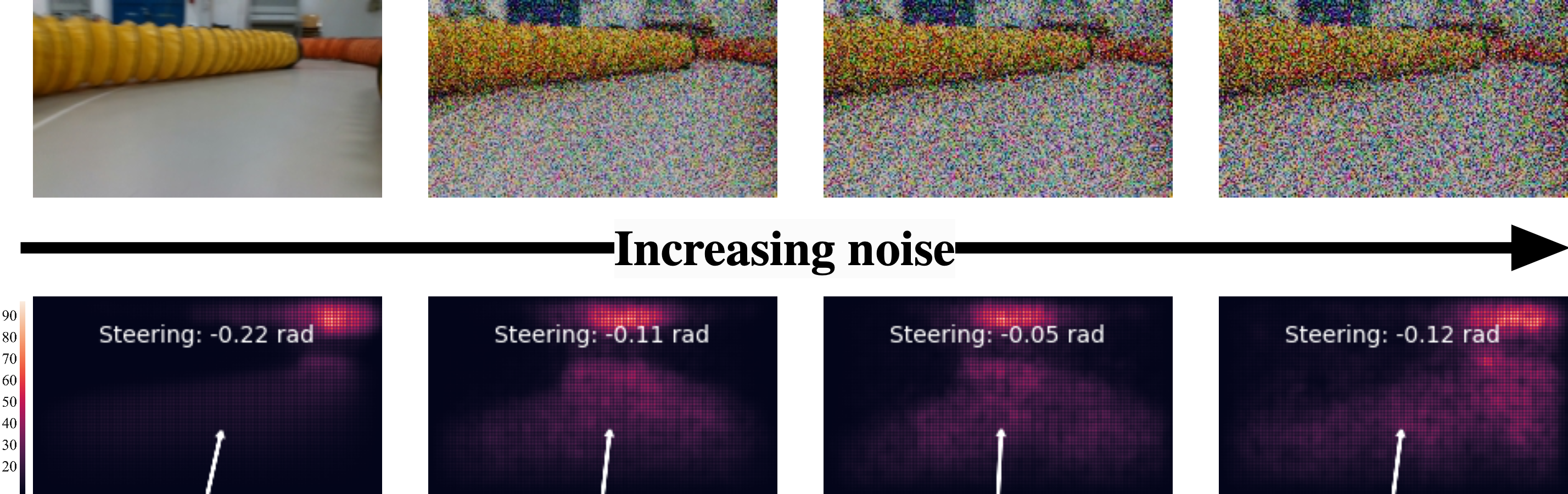
Figure 8: Attention maps during closed-loop testing, for input with no-noise and increased Gaussian noise with variance of $\sigma=0.1$, $0.2$ and $0.3$, respectively. Evaluated on the EARLY_LSTM model, as it was the best-performing model being able to receive additional increasing input noise. It demonstrates that the model could consistently maintain its attention on the same region.

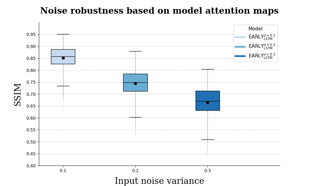
Figure 9: Robustness against noise during closed-loop testing, evaluated on the EARLY_LSTM model, which managed to maintain 100% autonomy without crashing, under increased noise. Here, we illustrate the SSIM index for attention maps between no-noise and increased Gaussian noise with variance of $\sigma=0.1$, $0.2$ and $0.3$, respectively.

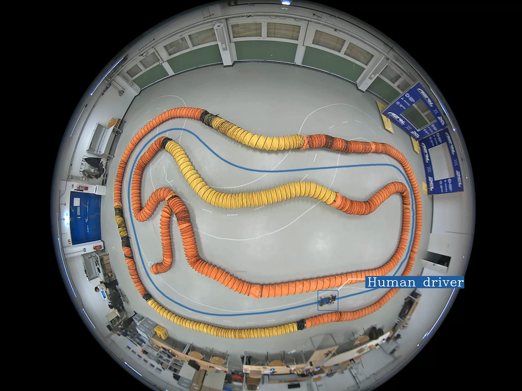
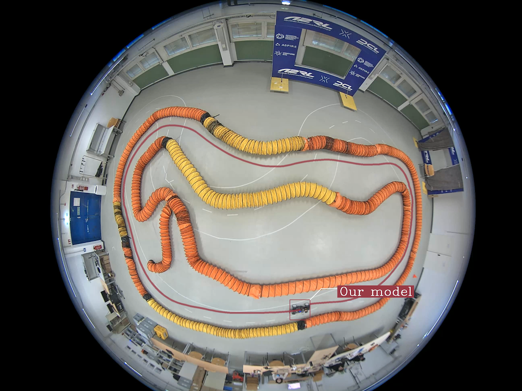
Figure 10: The trajectory of the human driver on the test track is shown on the left, while the trajectory of our best model, EARLY_LSTM, is shown on the right, both plotted using object tracking. While the model exhibits a smooth trajectory, it does not fully match the driving style of the human driver.

To analyze this quantitatively, we want to see how much the attention of these models gets distorted when extra noise is introduced. For this, we used the Structural Similarity Index (SSIM) [30], which assigns a score between 0 and 1 to measure the similarity between two images. In our case, these images represent pairwise comparisons of attention maps under noise-free and noisy conditions. SSIM values close to 1 indicate that the network’s attention remained unchanged, demonstrating its resilience. The SSIM values between the no-noise and $\sigma=0.1$-variance noise for these models are shown in Figure 7. The significantly higher SSIM value of the EARLY_LSTM supports our finding that it can tackle noise with more robust attention, while the other models failed under this condition.

To further assess the robustness of the promising EARLY_LSTM model, we gradually increased the noise level to 0.2 and then to 0.3. Impressively, the model remained robust even at these high noise levels. We were particularly interested in how this resilience relates to the model’s attention maps - specifically, how well it maintains focus on key input features without being distracted by noise during steering. This is shown in Figure 8.

The corresponding SSIM values are presented in Figure 9, which demonstrates that even with a high level of noise, the EARLY_LSTM managed to keep its attention similarity close to 1, with $86\%,75\%$ and $67\%$, respectively. Although there is a decrease in SSIM values as noise increases, the rate of decrease is not linear, it slows down progressively, with values decreasing by $-14\%$, $-11\%$, and $-8\%$, respectively. This suggests that while the model is affected by noise, it retains much of its attention stability even at higher noise levels. This resilience could be a key factor in its consistent performance under these challenging, noisy conditions.

V-D Comparison with Human Expert Driver

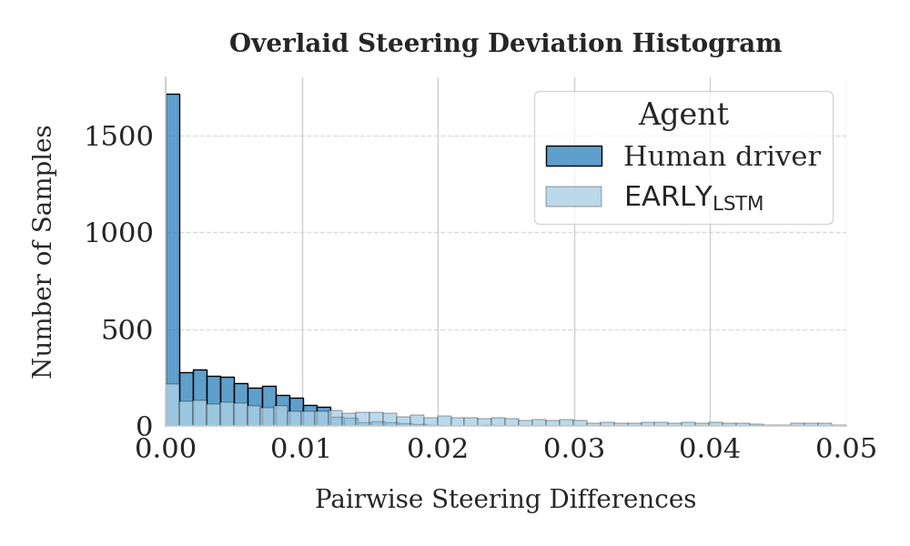
Figure 11: Histogram of steering differences between consecutive predictions, showing the smoothness of steering behavior. Values closer to zero indicate smoother steering. The plots compare the distribution between model predictions and human-commanded steering during closed-loop testing. On the left, the histogram represents real-time inference where $\approx 7$fps were being dropped due to hardware limitations. On the right, we plot the post-hoc inference results. The similarity between the two distributions suggests that frame drops did not significantly affect the model’s overall behavior.

After successfully deploying and testing the EARLY_LSTM model under various noisy conditions, we raised the question of how this model compares to human expert driver behavior. To explore this, we recorded a driving session of 5 continuous laps with the human driver on the test track.

To compare the driving trajectory of the human driver and the EARLY_LSTM model, we implemented an object tracking algorithm using OpenCV [31] that tracks the agent over time and plots its trajectory on the static test layout. This is shown in Figure 10. Although the model produces a very smooth trajectory, it does not fully replicate the exact human driver’s driving style. We hypothesize that this difference may be due to the experience the human driver possesses. Even though we used 5 different track layouts for training, we believe that incorporating even more layouts into the training pipeline could improve generalization, enabling the model to more closely match the performance of the human driver.

V-E Impact of Frame Drops on Model Performance

During real-time inference, our model experienced frame drops due to hardware limitations, resulting in a drop of approximately 7fps. Despite this, the model successfully completed 5 fully autonomous laps, including three test scenarios with added noise, all in a consistent manner.

To assess whether these frame drops influenced the model’s behavior, we reprocessed the recorded data offline on a virtual machine, ensuring that all frames were used for inference. Figure 11 compares the histogram of pairwise absolute steering differences between the model and the human driver under both conditions: (1) real-time inference with dropped frames and (2) post-hoc inference using all recorded frames. The similarity between the two distributions suggests that even frame drops did not introduce significant erratic behavior or deviation in the model’s predictions.

VI CONCLUSION

Overcoming the sim-to-real gap for autonomous agents poses many challenges. In our paper, we provided an in-depth analysis of our successful deployment of a multimodal RGB-D recurrent controller. During deployment, we found that depth information is crucial – the unimodal RGB feature extractor was insufficient for autonomous navigation, whereas we could successfully deploy a controller for each multimodal RGB-D feature extractor. Our early fusion LSTM agent maintained 100% autonomy in previously unseen scenarios and high resilience to both unpredictable data loss and increased input noise. In order to interpret the model behavior, we employed various numerical and visual techniques, which reinforced our observations from the closed-loop tests.

References

- [1] M. Lechner, R. Hasani, A. Amini, T. A. Henzinger, D. Rus, and R. Grosu, “Neural circuit policies enabling auditable autonomy,” Nature Machine Intelligence, vol. 2, no. 10, p. 642–652, Oct. 2020.
- [2] R. Hasani, M. Lechner, A. Amini, D. Rus, and R. Grosu, “Liquid time-constant networks,” in Proceedings of the AAAI Conference on Artificial Intelligence, vol. 35, no. 9, 2021, pp. 7657–7666.
- [3] R. Hasani, M. Lechner, A. Amini, L. Liebenwein, A. Ray, M. Tschaikowski, G. Teschl, and D. Rus, “Closed-form continuous-time neural networks,” Nature Machine Intelligence, vol. 4, no. 11, p. 992–1003, Nov. 2022. [Online]. Available: http://dx.doi.org/10.1038/s42256-022-00556-7
- [4] M. Farsang, S. A. Neubauer, and R. Grosu, “Liquid resistance liquid capacitance networks,” arXiv preprint arXiv:2403.08791, 2024.
- [5] M. Farsang, M. Lechner, D. Lung, R. Hasani, D. Rus, and R. Grosu, “Learning with chemical versus electrical synapses does it make a difference?” in 2024 IEEE International Conference on Robotics and Automation (ICRA), 2024, pp. 15 106–15 112.
- [6] D. Mújica-Vargas, A. Luna-Álvarez, M. Castro Bello, and A. A. Arenas Muñiz, RGB-D Convolutional Recurrent Neural Network to Control Simulated Self-driving Car. Cham: Springer Nature Switzerland, 2024, pp. 395–416. [Online]. Available: https://doi.org/10.1007/978-3-031-69769-2˙16
- [7] Y. Xiao, F. Codevilla, A. Gurram, O. Urfalioglu, and A. M. López, “Multimodal end-to-end autonomous driving,” CoRR, vol. abs/1906.03199, 2019. [Online]. Available: http://arxiv.org/abs/1906.03199
- [8] Ese6150: Roboracer autonomous racing cars. [Online]. Available: https://roboracer.ai/course
- [9] Y. Lecun, L. Bottou, Y. Bengio, and P. Haffner, “Gradient-based learning applied to document recognition,” Proceedings of the IEEE, vol. 86, no. 11, pp. 2278–2324, 1998.
- [10] W. Wang and U. Neumann, “Depth-aware CNN for RGB-D segmentation,” CoRR, vol. abs/1803.06791, 2018. [Online]. Available: http://arxiv.org/abs/1803.06791
- [11] J. Dai, H. Qi, Y. Xiong, Y. Li, G. Zhang, H. Hu, and Y. Wei, “Deformable convolutional networks,” CoRR, vol. abs/1703.06211, 2017. [Online]. Available: http://arxiv.org/abs/1703.06211
- [12] X. Zhu, H. Hu, S. Lin, and J. Dai, “Deformable convnets v2: More deformable, better results,” 2018. [Online]. Available: https://arxiv.org/abs/1811.11168
- [13] Z. Wu, G. Allibert, C. Stolz, and C. Demonceaux, “Depth-adapted cnn for rgb-d cameras,” 2020. [Online]. Available: https://arxiv.org/abs/2009.09976
- [14] M. Bojarski, D. D. Testa, D. Dworakowski, B. Firner, B. Flepp, P. Goyal, L. D. Jackel, M. Monfort, U. Muller, J. Zhang, X. Zhang, J. Zhao, and K. Zieba, “End to end learning for self-driving cars,” CoRR, vol. abs/1604.07316, 2016. [Online]. Available: http://arxiv.org/abs/1604.07316
- [15] Y. Zhang, R. Ge, L. Lyu, J. Zhang, C. Lyu, and X. Yang, “A virtual end-to-end learning system for robot navigation based on temporal dependencies,” IEEE Access, vol. 8, pp. 134 111–134 123, 2020.
- [16] S. Hochreiter and J. Schmidhuber, “Long short-term memory,” Neural computation, vol. 9, pp. 1735–80, 12 1997.
- [17] F. Makiyeh, M. Bastourous, A. Bairouk, W. Xiao, M. Maras, T.-H. Wangb, M. Blanchon, R. Hasani, P. Chareyre, and D. Rus, “Optical flow matters: an empirical comparative study on fusing monocular extracted modalities for better steering,” 2024. [Online]. Available: https://arxiv.org/abs/2409.12716
- [18] B. D. Evans, J. Betz, H. Zheng, H. A. Engelbrecht, R. Mangharam, and H. W. Jordaan, “Bypassing the simulation-to-reality gap: Online reinforcement learning using a supervisor,” 2023. [Online]. Available: https://arxiv.org/abs/2209.11082
- [19] B. D. Evans, H. W. Jordaan, and H. A. Engelbrecht, “Safe reinforcement learning for high-speed autonomous racing,” Cognitive Robotics, vol. 3, pp. 107–126, 2023. [Online]. Available: https://www.sciencedirect.com/science/article/pii/S2667241323000125
- [20] H. W. J. Benjamin David Evans and H. A. Engelbrecht, “Comparing deep reinforcement learning architectures for autonomous racing,” Machine Learning with Applications, vol. 14, p. 100496, 2023. [Online]. Available: https://www.sciencedirect.com/science/article/pii/S266682702300049X
- [21] M. M. Zarrar, Q. Weng, B. Yerjan, A. Soyyigit, and H. Yun, “Tinylidarnet: 2d lidar-based end-to-end deep learning model for f1tenth autonomous racing,” 2024. [Online]. Available: https://arxiv.org/abs/2410.07447
- [22] M. Loetscher, N. Baumann, E. Ghignone, A. Ronco, and M. Magno, “Assessing the robustness of lidar, radar and depth cameras against ill-reflecting surfaces in autonomous vehicles: An experimental study,” 2023. [Online]. Available: https://arxiv.org/abs/2309.10504
- [23] J. Betz, H. Zheng, F. Jahncke, Z. Zang, F. Sauerbeck, Y. R. Zheng, J. Biswas, V. Krovi, and R. Mangharam, “F1tenth: Enhancing autonomous systems education through hands-on learning and competition,” IEEE Transactions on Intelligent Vehicles, pp. 1–13, 2024.
- [24] F. Resch, “Autonomous racing with attention-based neural networks,” Master’s thesis, Technische Universität Wien, 2023.
- [25] C. Lanczos, “An iteration method for the solution of the eigenvalue problem of linear differential and integral operators,” Journal of research of the National Bureau of Standards, vol. 45, no. 4, pp. 255–282, 1950.
- [26] E. Catmull and R. Rom, “A class of local interpolating splines,” in Computer aided geometric design. Elsevier, 1974, pp. 317–326.
- [27] A. Eitel, J. T. Springenberg, L. Spinello, M. A. Riedmiller, and W. Burgard, “Multimodal deep learning for robust RGB-D object recognition,” CoRR, vol. abs/1507.06821, 2015. [Online]. Available: http://arxiv.org/abs/1507.06821
- [28] D. P. Kingma and J. Ba, “Adam: A method for stochastic optimization,” arXiv preprint arXiv:1412.6980, 2014.
- [29] M. Bojarski, A. Choromanska, K. Choromanski, B. Firner, L. D. Jackel, U. Muller, and K. Zieba, “Visualbackprop: visualizing cnns for autonomous driving,” CoRR, vol. abs/1611.05418, 2016. [Online]. Available: http://arxiv.org/abs/1611.05418
- [30] Z. Wang, A. Bovik, H. Sheikh, and E. Simoncelli, “Image quality assessment: from error visibility to structural similarity,” IEEE Transactions on Image Processing, vol. 13, no. 4, pp. 600–612, 2004.
- [31] G. Bradski, “The OpenCV Library,” Dr. Dobb’s Journal of Software Tools, 2000.