Lower limit of percolation threshold on a square lattice with complex neighborhoods

Abstract

In this paper, the 60-year-old concept of long-range interaction in percolation problems introduced by Dalton, Domb, and Sykes, is reconsidered. With Monte Carlo simulation—based on Newman–Ziff algorithm and finite-size scaling hypothesis—we estimate 64 percolation thresholds for random site percolation problem on a square lattice with neighborhoods that contain sites from the 7th coordination zone. The percolation thresholds obtained range from $0.27013$ (for the neighborhood that contains only sites from the 7th coordination zone) to $0.11535$ (for the neighborhood that contains all sites from the 1st to the 7th coordination zone). Similarly to neighborhoods with smaller ranges, the power-law dependence of the percolation threshold on the effective coordination number with exponent close to $-1/2$ is observed. Finally, we empirically determine the limit of the percolation threshold on square lattices with complex neighborhoods. This limit scales with the inverse square of the mean radius of the neighborhood. The boundary of this limit is touched for threshold values associated with extended (compact) neighborhoods.

I Introduction

The percolation [1, 2, 3, 4] (see References [5, 6] for recent reviews) is one of the core topics in statistical physics providing the possibility to look at the critical phenomena occurring at phase transition solely on the geometrical basis, without samples heating, cooling, inserting in a magnetic field, etc. Some problems with respect to percolation can be treated analytically [7, 8, 9, 10, 11, 12], but most studies are computational.

Originating from works by Broadbent and Hammersley [13, 14] devoted to rheology (and still applied there [15, 16, 17, 18]), it quickly found plenty of applications in physics, including magnetic [19, 20, 21, 22, 23] and electric [24, 25, 26] properties of solids or nano-engineering [27].

However, the application of percolation theory is not restricted to physics alone. Such examples (mainly two-dimensional systems [28, 29, 30, 31, 32]) can also be found in epidemiology [33, 34, 35], forest fires [36, 37, 38, 39, 40], agriculture [41, 42, 43], urbanization [44, 45], materials chemistry [46], sociology [47], psychology [48], information transfer [49], finances [50], or dentistry [51].

On the other hand, some effort was put into studying percolation on cubic ($d=3$ [52, 53, 54, 55, 56, 57]) and hyper-cubic lattices, also for non-physical dimensions ($d=4$ [58, 52, 59, 60], $d=5$ [61, 52, 60] and higher $d\geq 6$ [62, 52, 63]). Simultaneously, the complex [6, 49, 64], distorted [65, 66, 67] and fractal [68] networks were studied.

Recently, the 60-year-old concept of long-range interaction [69, 70] has sparked renewed interest. The neighborhood that contains sites that are not nearest-neighbors on assumed lattice are called extended neighborhoods (when they are compact) or complex (when they are non-compact, that is, they contain ‘wholes’)—to keep the nomenclature from Reference [71]. Many papers were devoted to studies of the percolation thresholds on the extended [72, 73, 59, 74, 49, 61] and the complex [75, 76, 77, 57, 78, 58, 79, 80, 81, 82, 71] neighborhoods.

The particular neighborhoods names—now keeping the convention proposed in Reference [83]—are combination of alphanumeric strings. The first two letters identify the underlying lattice (for example: sq for square, tr for triangular, hc for honeycomb, and sc for simple cubic lattices) then they are accompanied with numerical string indicating coordination zones which constitute the neighborhood. In this convention, the von Neumann neighborhood on the square lattice (with only the nearest neighbors) is called sq-1, while Moore’s neighborhood on square lattice (containing sites from the first and the second coordination zones) is called sq-1,2.

In this paper we are closer to the theoretical studies of percolation phenomena than to its application. That is, our studies focus on the influence of long-range interactions on the percolation threshold $p_{c}$. The percolation threshold is the equivalent of the critical point in the phase-transition phenomena. For the random site percolation problem, we deal with the nodes of the lattice that are occupied (with probability $p$) or empty (with probability $1-p$). Occupied sites, in assumed neighborhood, are considered to form a cluster. Depending on the sites occupation probability $p$ such cluster may span (or not) the system edges. The percolation threshold $p_{c}$ is such an occupation probability $p$, that for $p<p_{c}$ a spanning cluster is absent (and the system behaves as an insulator), while for $p>p_{c}$ a spanning cluster is present (and the system behaves as a conductor). Thus, $p_{c}$ separates two phases: isolating and conducting, and at $p=p_{c}$ the (second-order) phase transition takes place.

Here, we calculate the percolation thresholds $p_{c}$ for random site percolation in the square lattice for neighborhoods containing sites from the 7th coordination zone. There are 64 such neighborhoods, from sq-7 to sq-1,2,3,4,5,6,7, and they are presented in Figure˜1.

The paper is organized as follows: in Section˜II we recall the finite-size scaling hypothesis, present basics of the effective Newman–Ziff Monte Carlo algorithm for the percolation problem, define the effective coordination number and give some details regarding technicalities of computations. In Section˜III we show the results of Monte Carlo simulations which allow for the estimation of 64 values of $p_{c}$ for various neighborhoods together with their geometrical characteristics, such as total and effective coordination numbers. Finally, Section˜IV is devoted to a discussion of the obtained results.

(a)

(b)

(c)

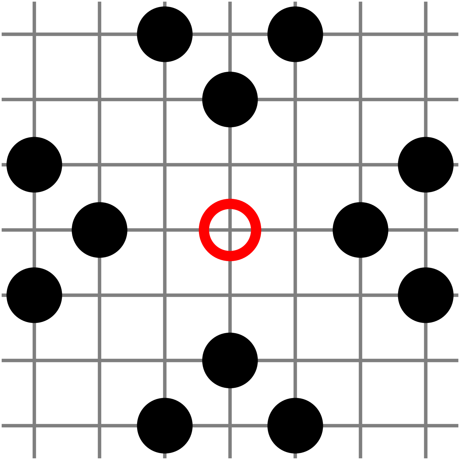
(d)

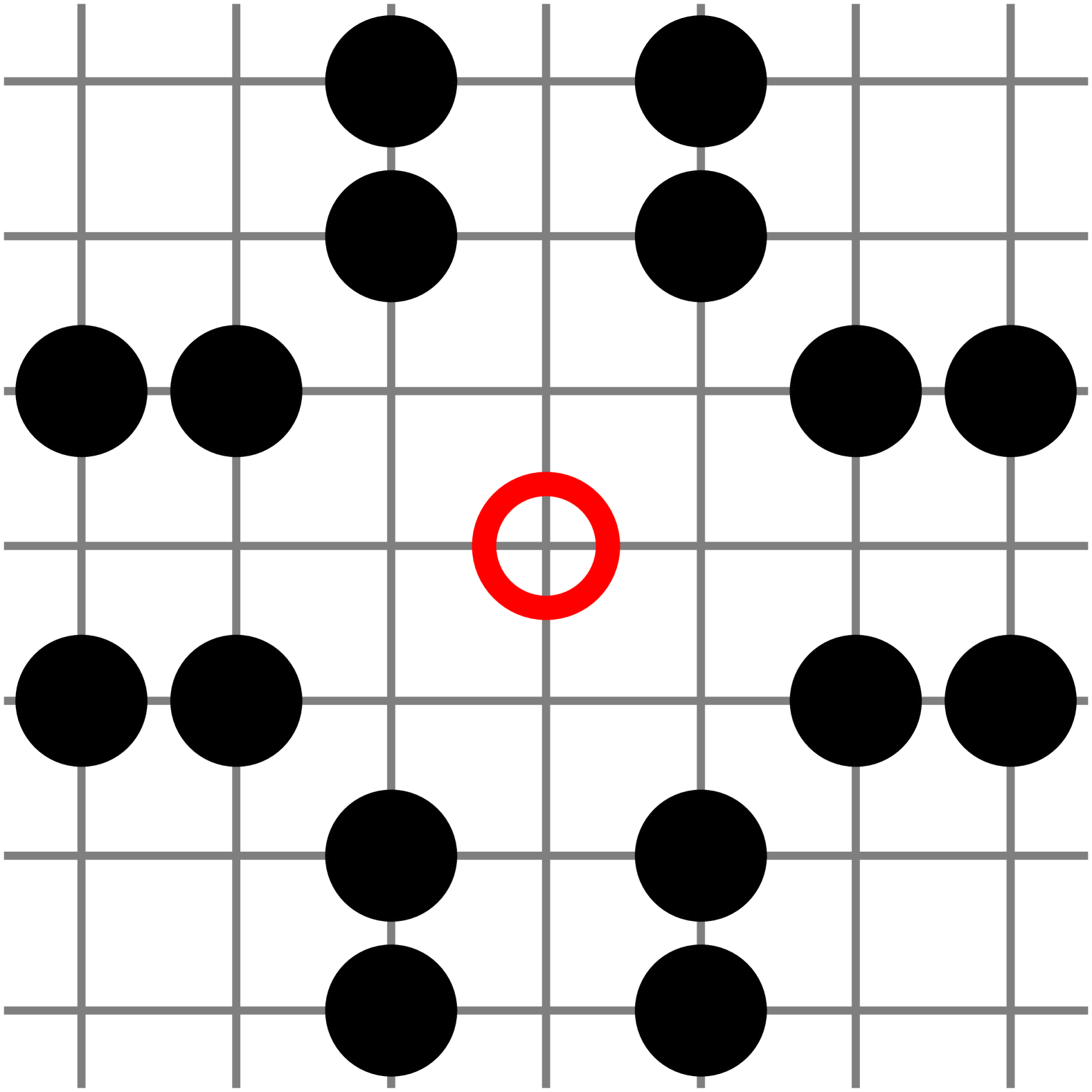
(e)

(f)

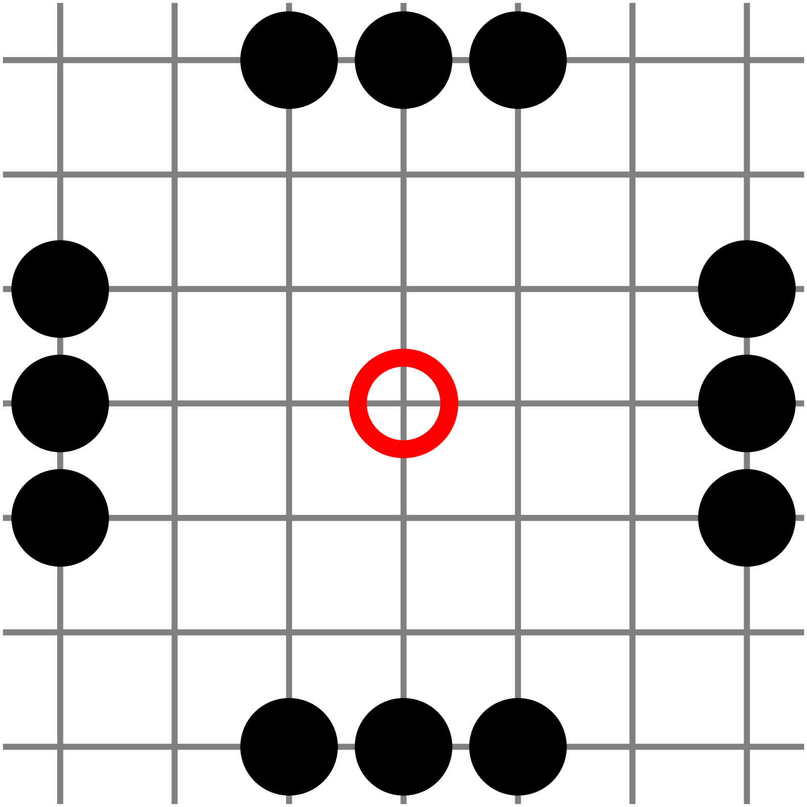
(g)

(h)

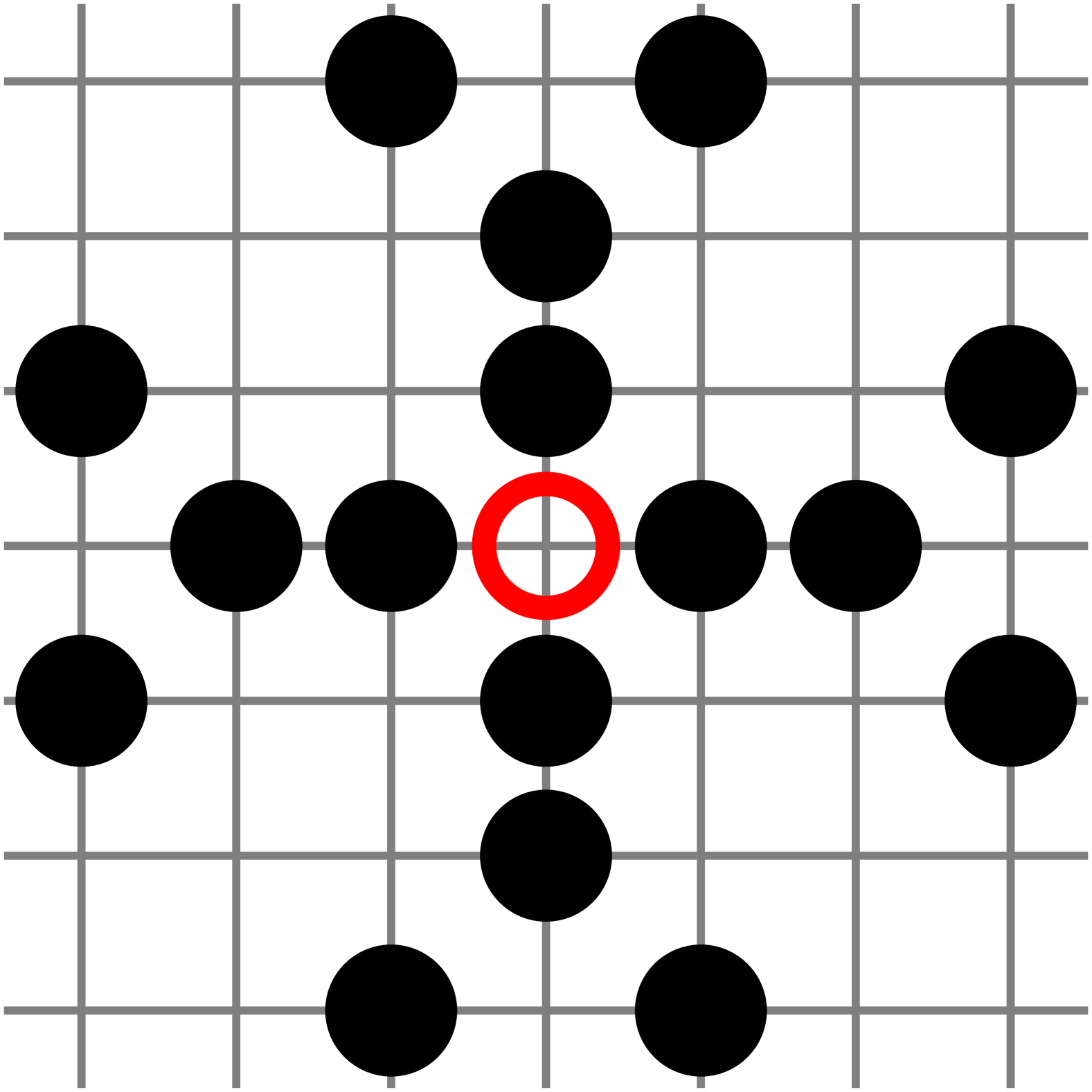
(i)

(j)

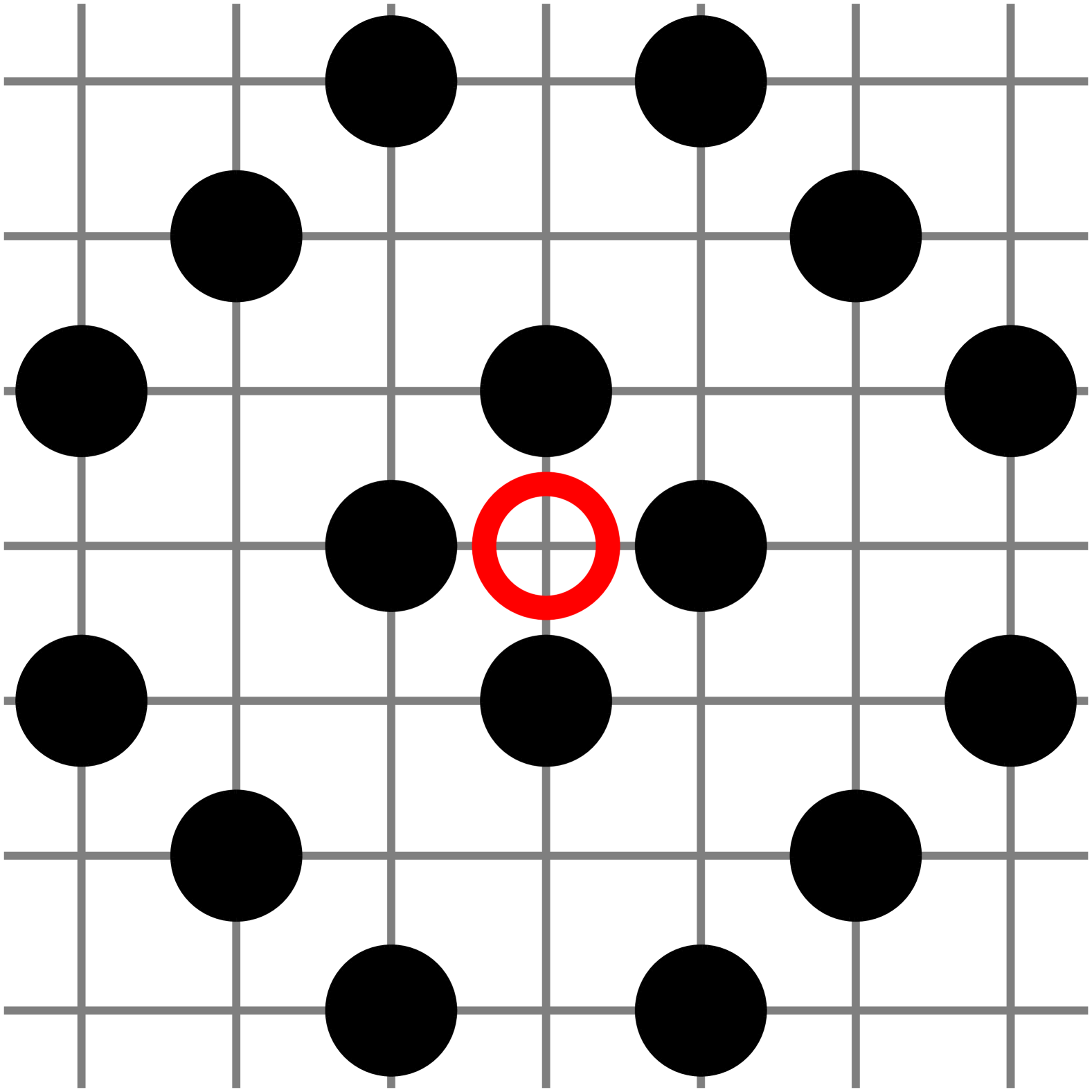
(k)

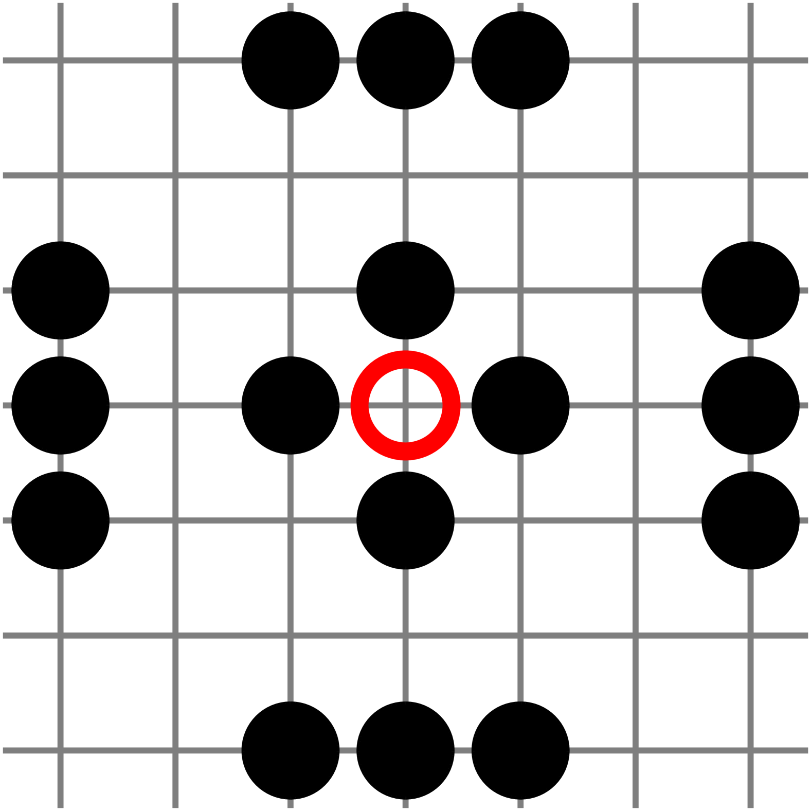
(l)

(m)

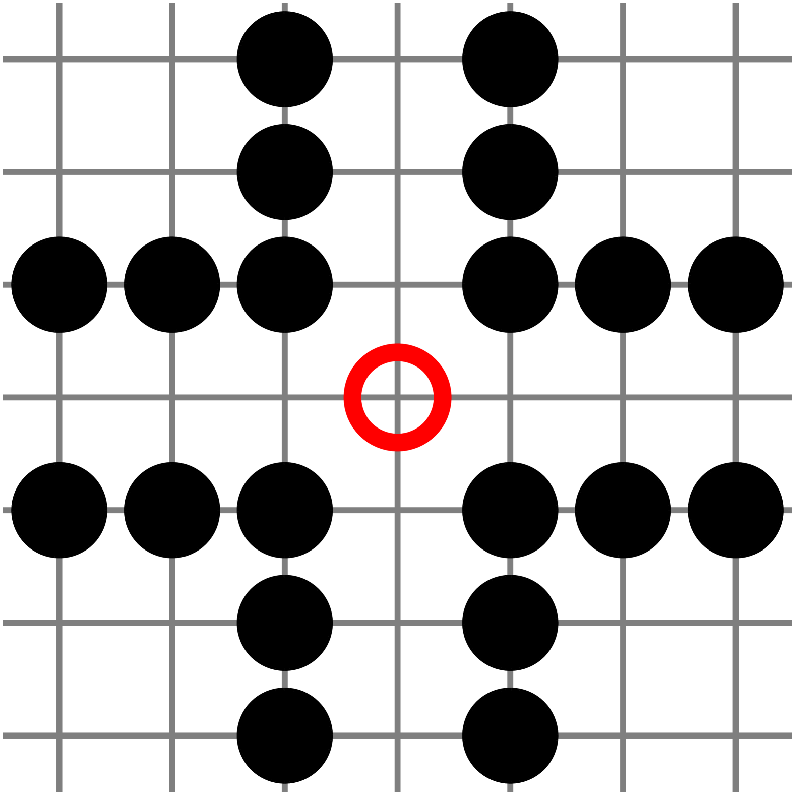
(n)

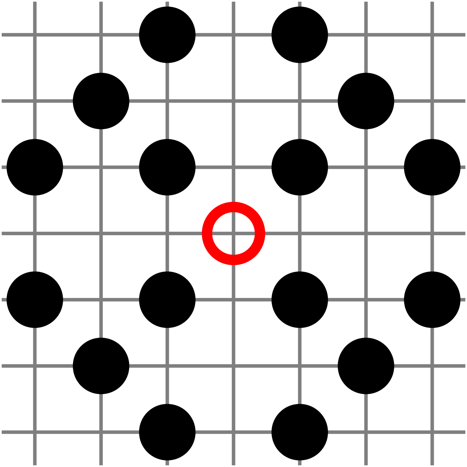
(o)

(p)

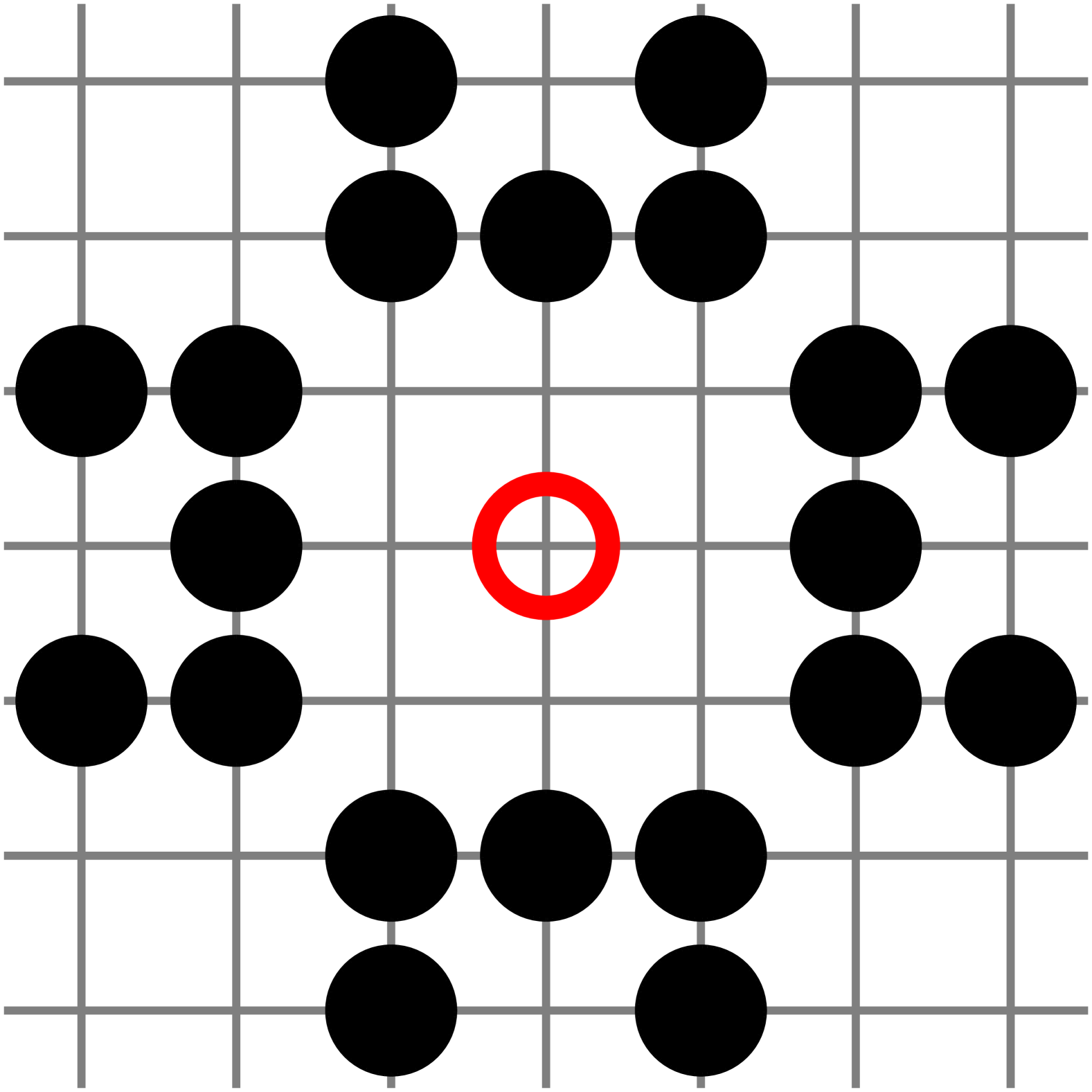
(q)

(r)

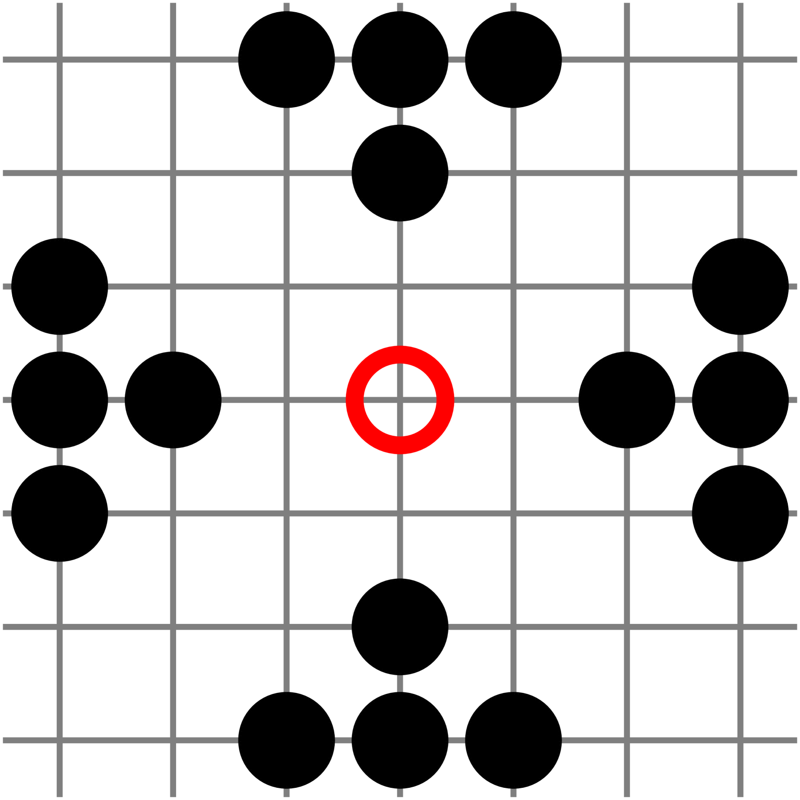
(s)

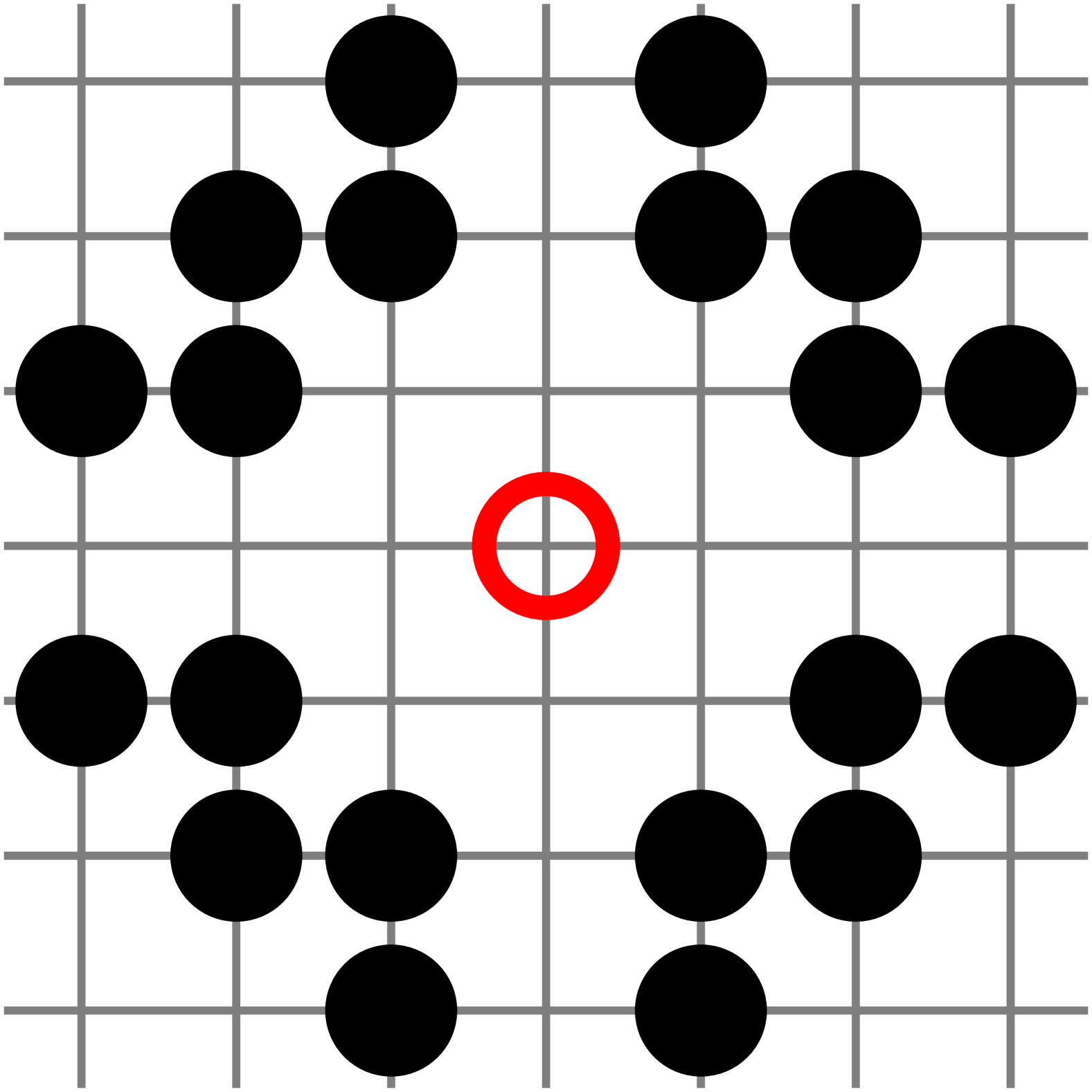
(t)

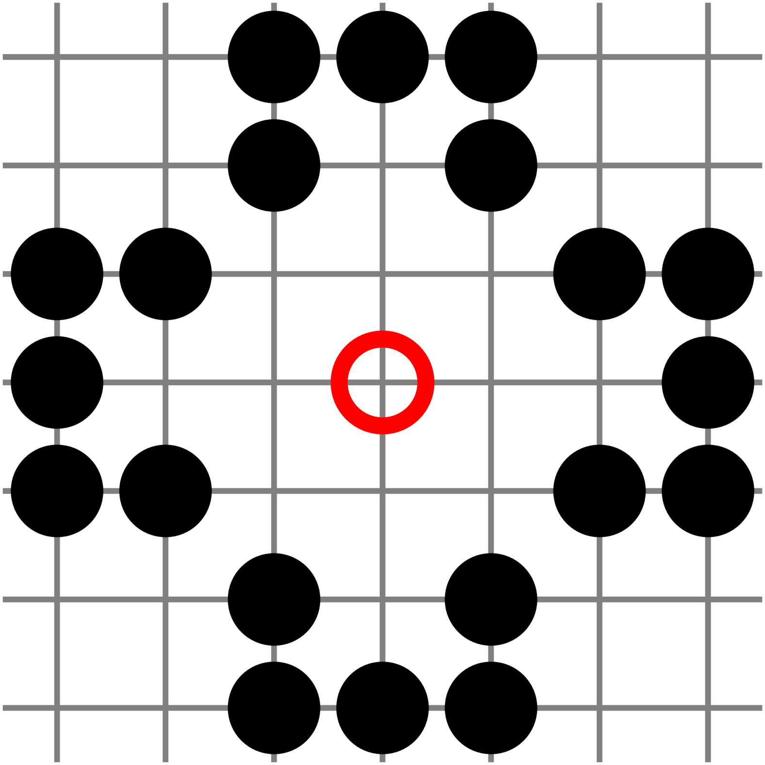
(u)

(v)

(w)

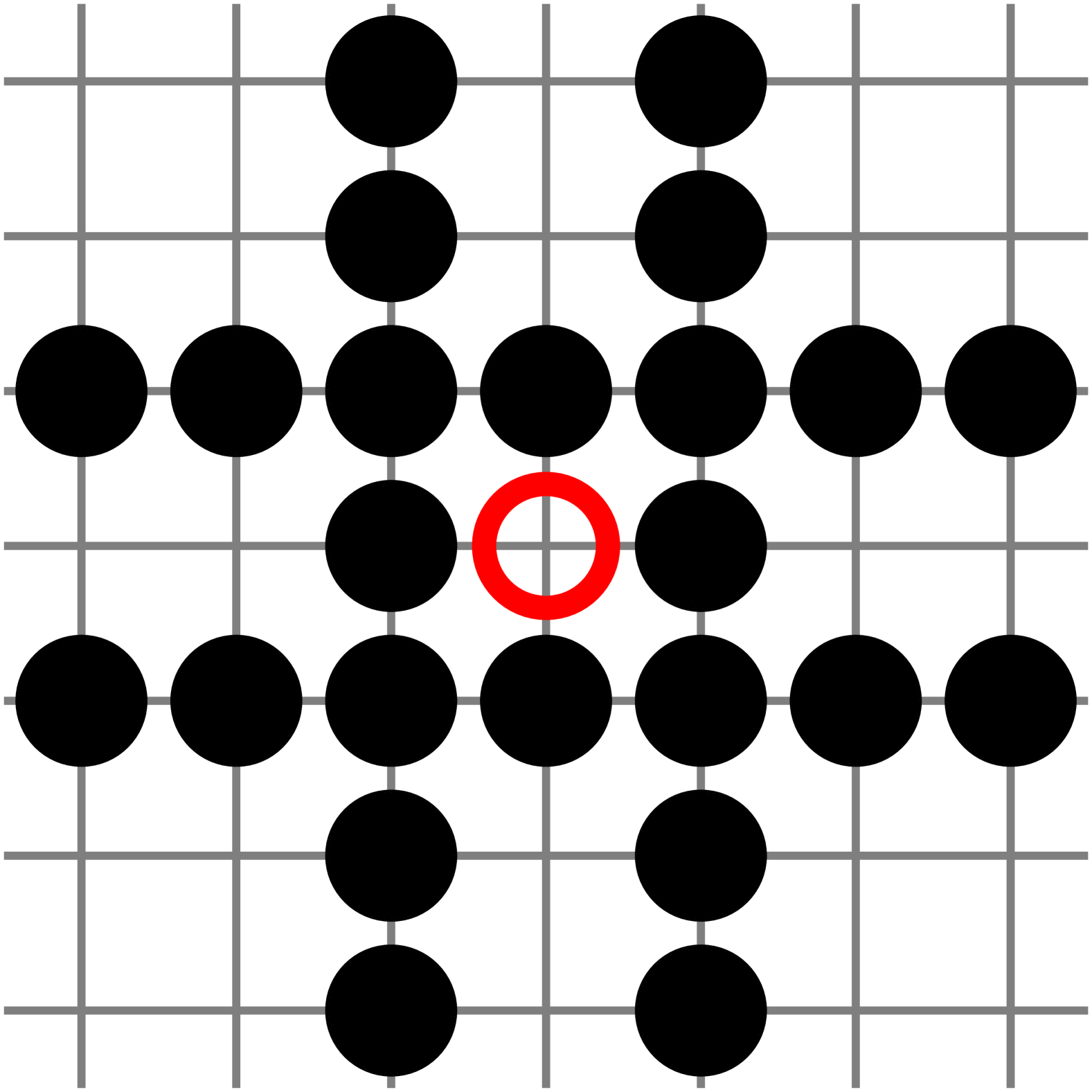
(x)

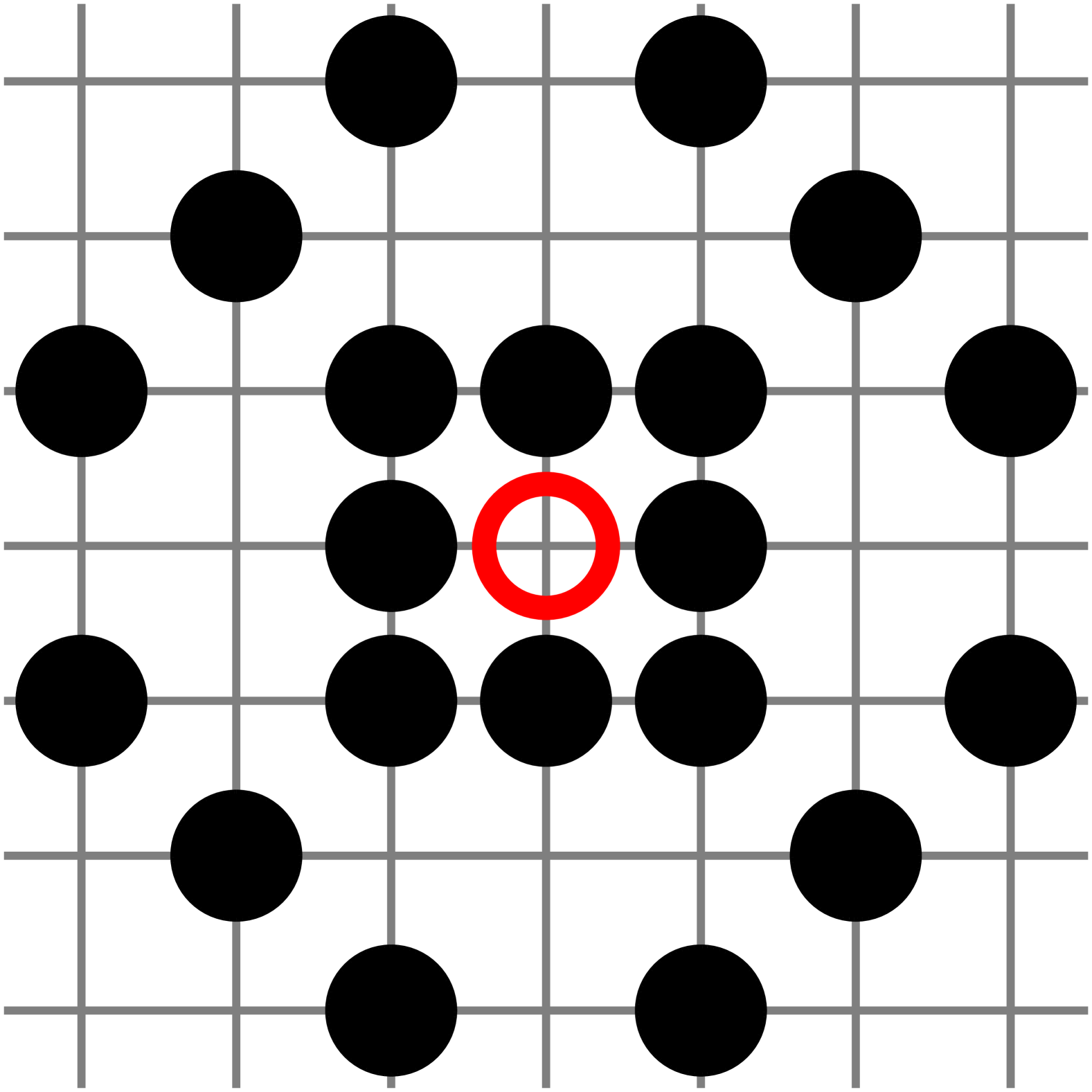
(y)

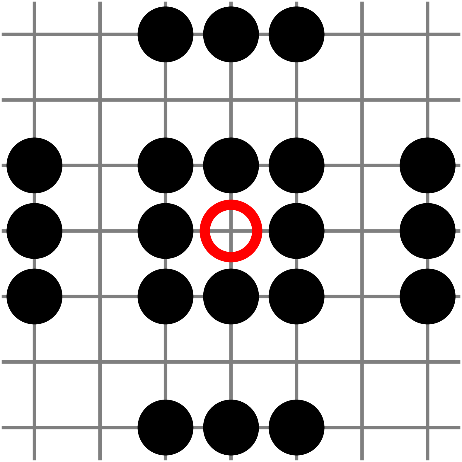
(z)

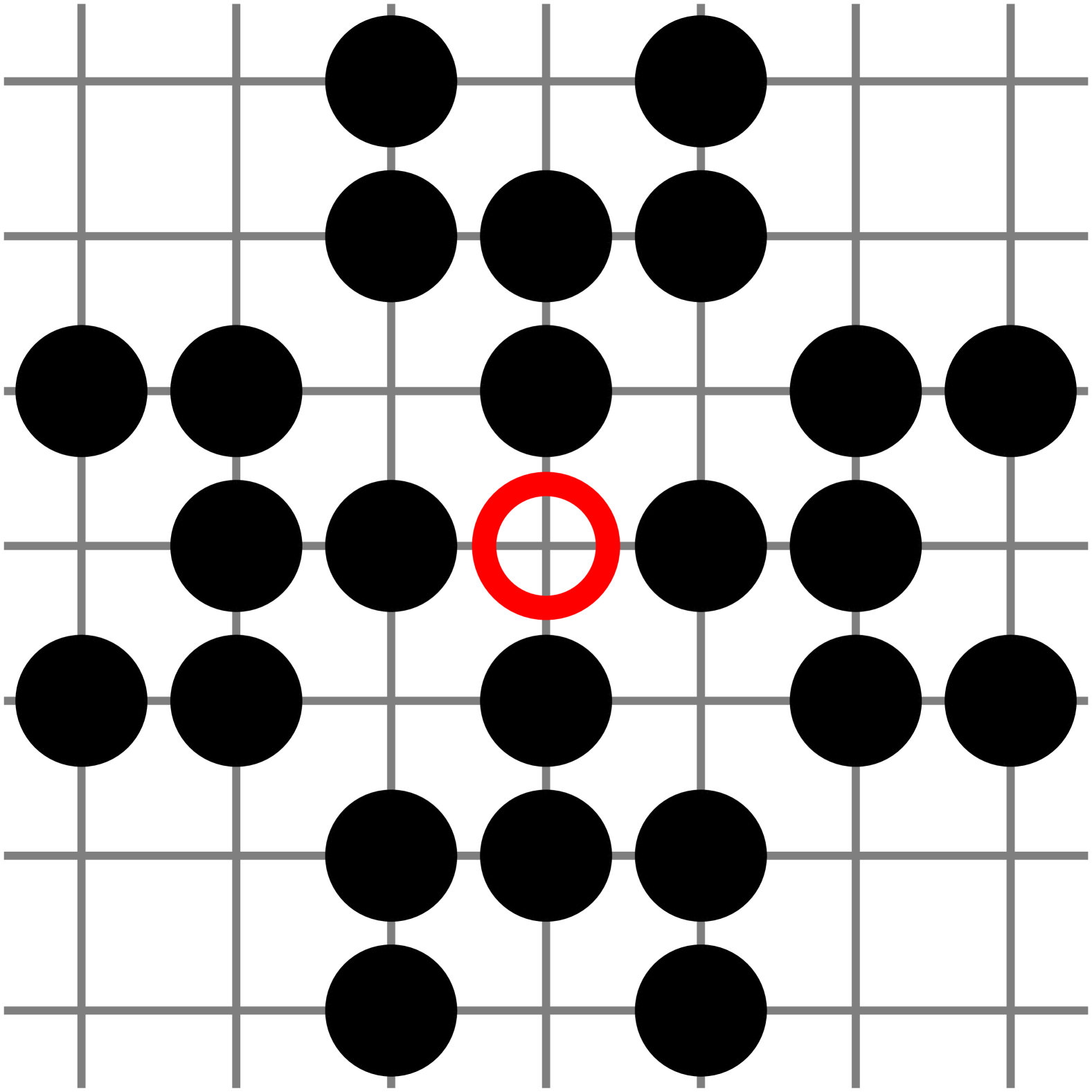
(aa)

(ab)

(ac)

(ad)

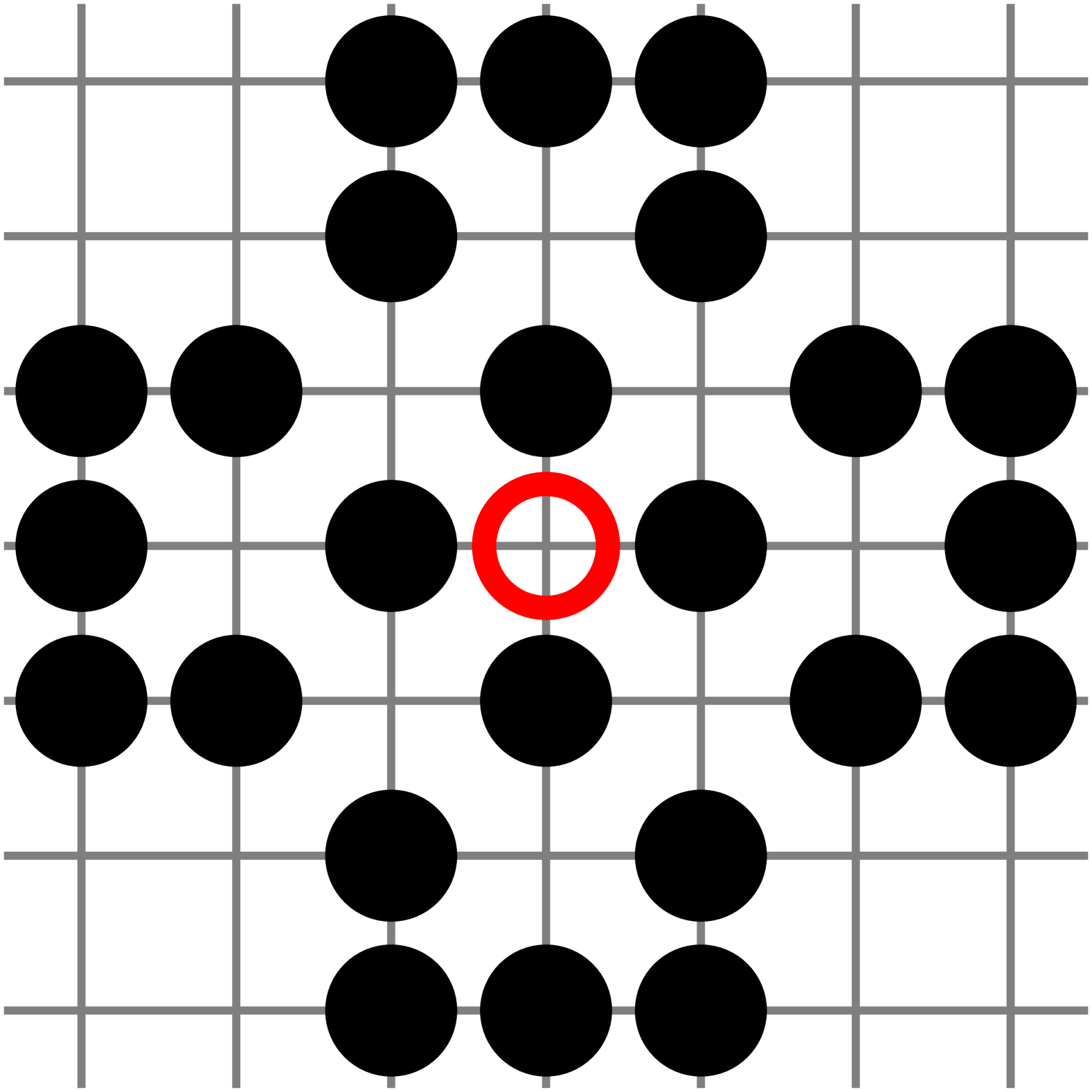
(ae)

(af)

(ag)

(ah)

(ai)

(aj)

(ak)

(al)

(am)

(an)

(ao)

(ap)

(aq)

(ar)

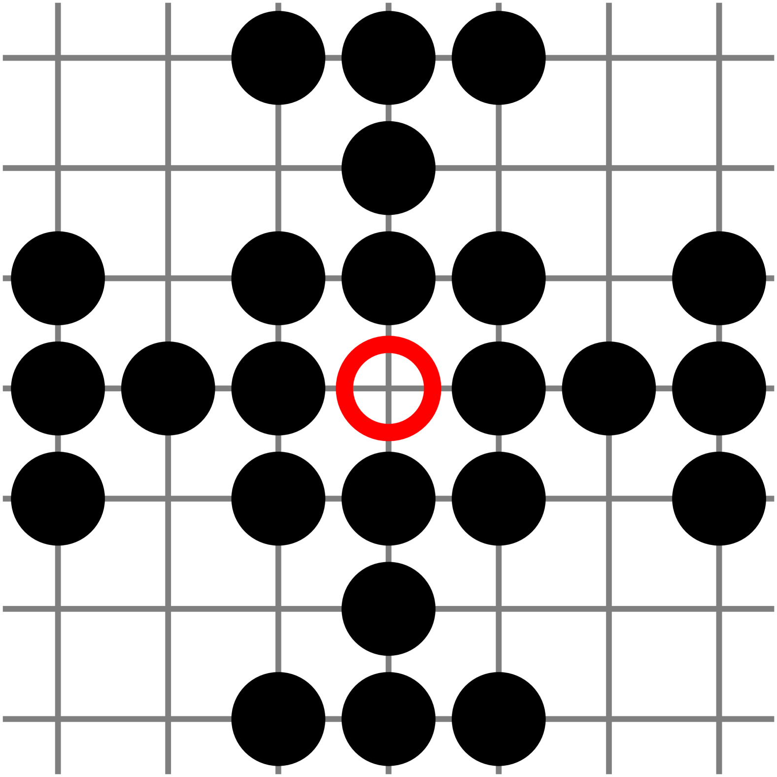
(as)

(at)

(au)

(av)

(aw)

(ax)

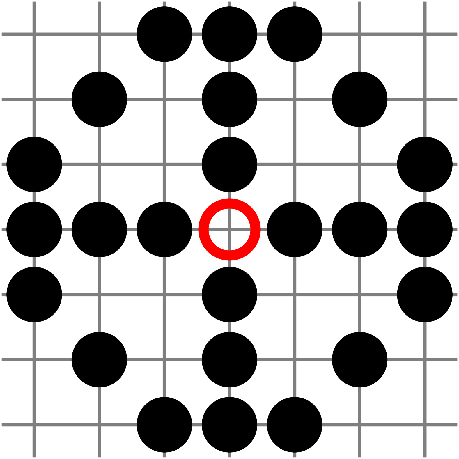
(ay)

(az)

(ba)

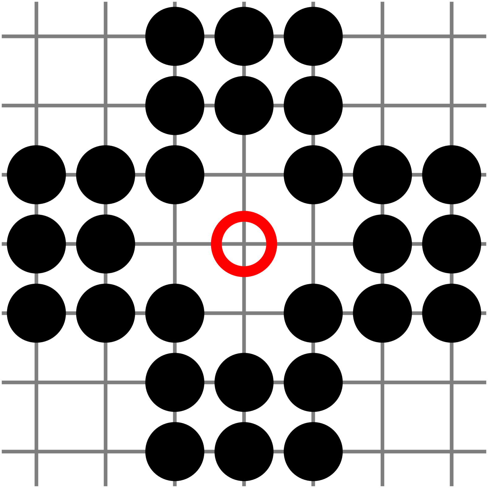
(bb)

(bc)

(bd)

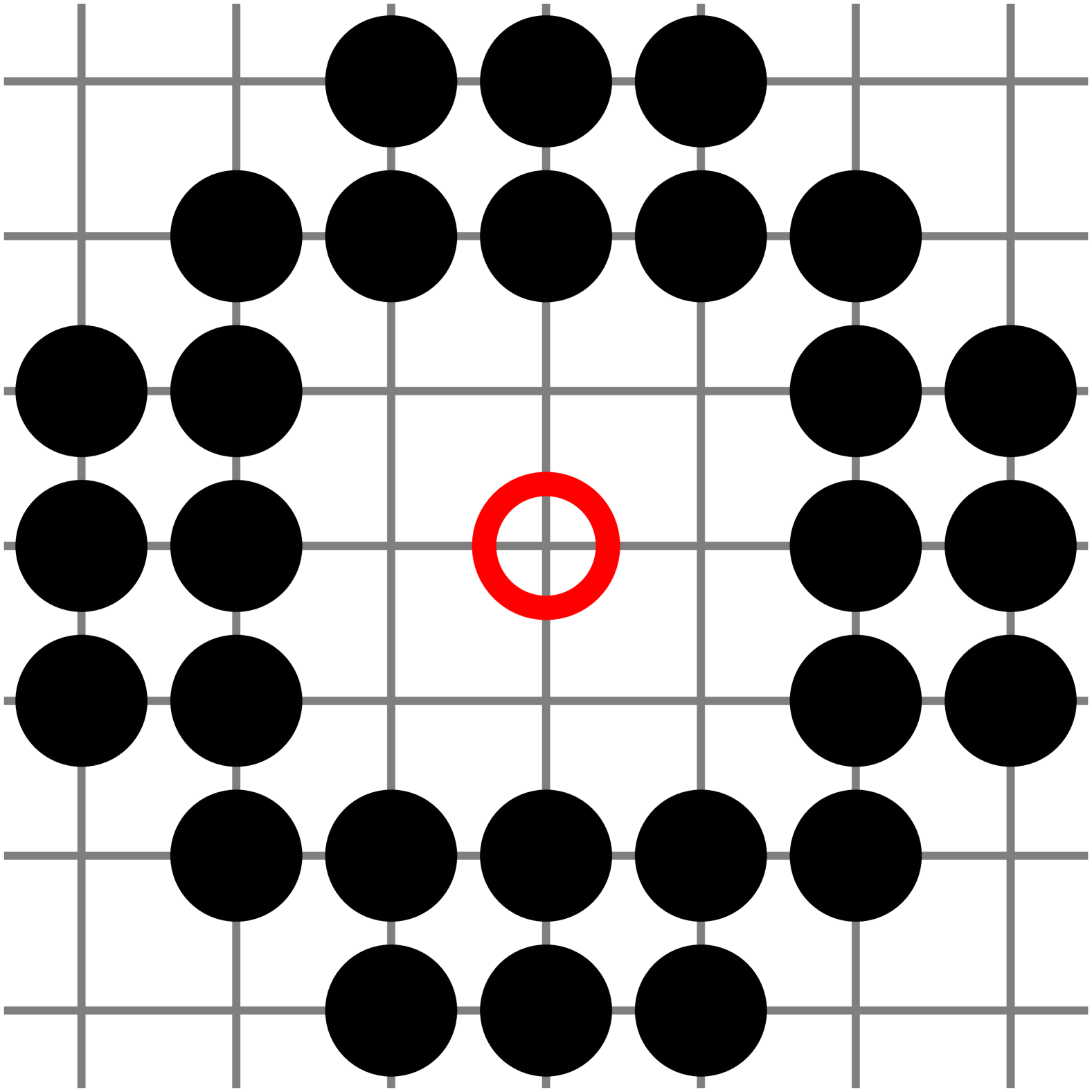
(be)

(bf)

(bg)

(bh)

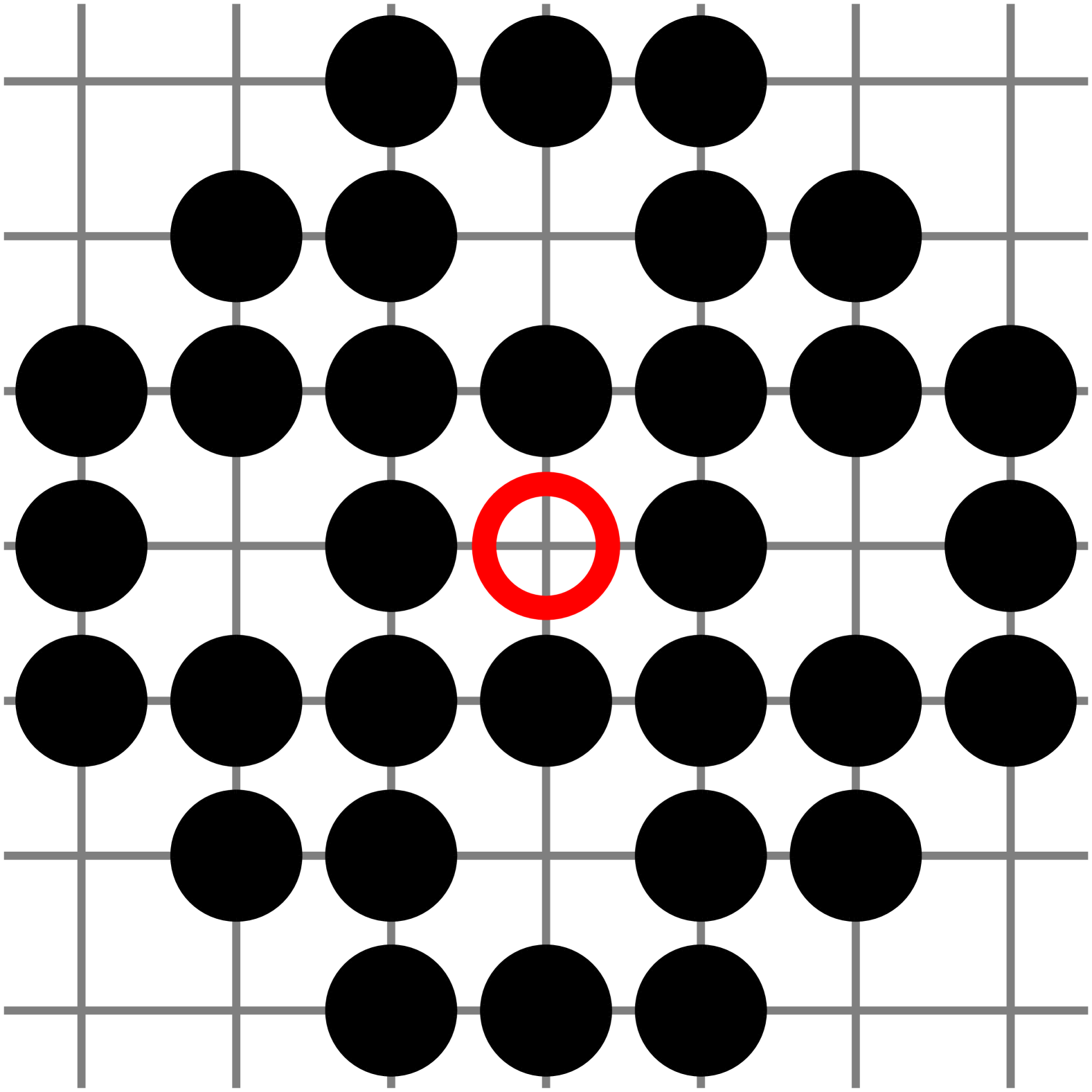
(bi)

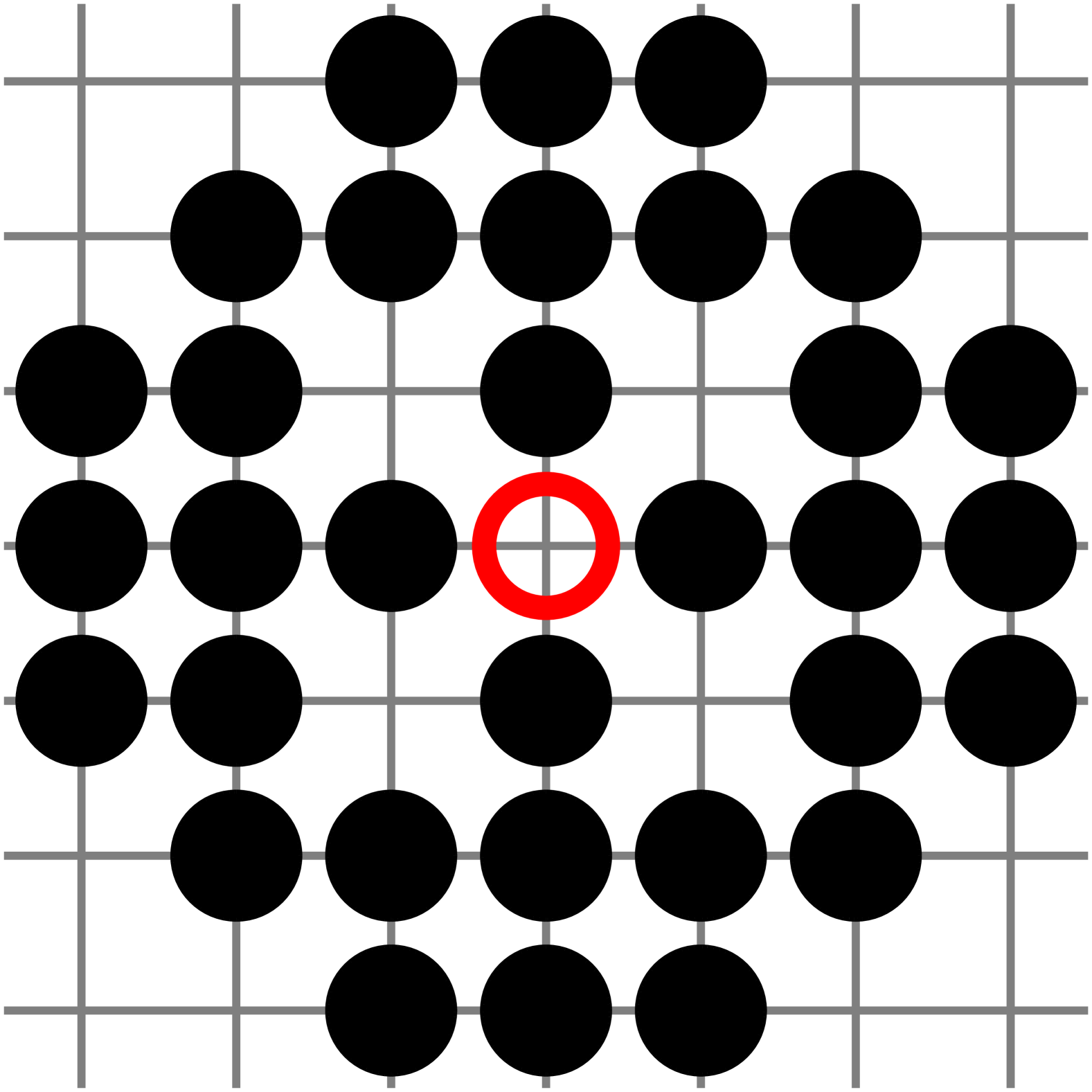
(bj)

(bk)

(bl)

Figure 1: Neighborhoods on square lattice containing sites from the 7-th coordination zone: (1(a)) sq-7, (1(b)) sq-1,7, (1(c)) sq-2,7, (1(d)) sq-3,7, (1(e)) sq-4,7, (1(f)) sq-5,7, (1(g)) sq-6,7, (1(h)) sq-1,2,7, (1(k)) sq-1,5,7, (1(l)) sq-1,6,7, (1(m)) sq-2,3,7, (1(n)) sq-2,4,7, (1(o)) sq-2,5,7, (1(p)) sq-2,6,7, (1(q)) sq-3,4,7, (1(r)) sq-3,5,7, (1(s)) sq-3,6,7, (1(t)) sq-4,5,7, (1(u)) sq-4,6,7, (1(v)) sq-5,6,7, (1(w)) sq-1,2,3,7, (1(x)) sq-1,2,4,7, (1(y)) sq-1,2,5,7, (1(z)) sq-1,2,6,7, (1(aa)) sq-1,3,4,7, (1(ab)) sq-1,3,5,7, (1(ac)) sq-1,3,6,7, (1(ad)) sq-1,4,5,7, (1(ae)) sq-1,4,6,7, (1(af)) sq-1,5,6,7, (1(ag)) sq-2,3,4,7, (1(ah)) sq-2,3,5,7, (1(ai)) sq-2,3,6,7, (1(aj)) sq-2,4,5,7, (1(ak)) sq-2,4,6,7, (1(al)) sq-2,5,6,7, (1(am)) sq-3,4,5,7, (1(an)) sq-3,4,6,7, (1(ao)) sq-3,5,6,7, (1(ap)) sq-4,5,6,7, (1(aq)) sq-1,2,3,4,7, (1(ar)) sq-1,2,3,5,7, (1(as)) sq-1,2,3,6,7, (1(at)) sq-1,2,4,5,7, (1(au)) sq-1,2,4,6,7, (1(av)) sq-1,2,5,6,7, (1(aw)) sq-1,3,4,5,7, (1(ax)) sq-1,3,4,6,7, (1(ay)) sq-1,3,5,6,7, (1(az)) sq-1,4,5,6,7, (1(ba)) sq-2,3,4,5,7, (1(bb)) sq-2,3,4,6,7, (1(bc)) sq-2,3,5,6,7, (1(bd)) sq-2,4,5,6,7, (1(be)) sq-3,4,5,6,7, (1(bf)) sq-1,2,3,4,5,7, (1(bg)) sq-1,2,3,4,6,7, (1(bh)) sq-1,2,3,5,6,7, (1(bi)) sq-1,2,4,5,6,7, (1(bj)) sq-1,3,4,5,6,7, (1(bk)) sq-2,3,4,5,6,7, (1(bl)) sq-1,2,3,4,5,6,7

II Methods

II.1 Finite-Size Scaling Hypothesis

In the vicinity of the critical point $x_{c}$, many observables $X$ obey the finite-size scaling [84, 1, 85] relation

$$X(x;L)=L^{-\varepsilon_{1}}\cdot\mathcal{F}\big{(}(x-x_{c})L^{\varepsilon_{2}}\big{)},$$ (1)

where $x$ reflects the level of system disorder, $\mathcal{F}$ is the scaling function (usually analytically unknown), and $\varepsilon_{1,2}$ are universal exponents. These exponents depend only on the physical dimension of the system $d$. Knowing $\varepsilon_{1,2}$ and plotting $X(x;L)$ leads to the collapse of many curves (for various $L$) into a single one.

At the critical point $x=x_{c}$, the value of

$$X(x=x_{c};L)\cdot L^{\varepsilon_{1}}=\mathcal{F}\big{(}0\big{)}$$ (2)

does not depend on the size of the system $L$, which opens a computationally feasible way of searching for both the critical point $x_{c}$ and the critical exponents $\varepsilon_{1,2}$.

For the random site percolation problem, the probability

$$P_{\text{max}}=S_{\text{max}}/L^{2},$$ (3)

that the randomly chosen site belongs to the largest cluster (with size $S_{\text{max}}$), may play the role of the quantity $X$. Then, the exponents $\varepsilon_{1,2}$ are known analytically, and $\varepsilon_{1}=5/48$ while $\varepsilon_{2}=3/4$.

II.2 Efficient Newman–Ziff Algorithm

To calculate the probability $P_{\text{max}}$ mentioned above we use Newman and Ziff algorithm [86]. The algorithm is fast as it is based on the concept of calculating desired quantities only after adding a single occupied site to the so far existing system. This allows us to construct the dependence of $X(n)$, where $n$ is the number of occupied sites.

The second part of the algorithm is the transformation of $X(n)$ values from the space of the integer number $n$ of occupied sites to $X(p)$ in the space of the real numbers of probabilities $p$ of sites occupation

$$X(p;N)=\sum_{n=0}^{N}\bar{X}(n;N)\mathcal{B}(n;N,p),$$ (4)

where $N=L^{2}$ stands for the size of the system. This conversion requires knowing the Bernoulli (binomial) probability distribution

$$\mathcal{B}(n;N,p)=\binom{N}{n}p^{n}(1-p)^{N-n}$$ (5)

and Reference [86] provides an efficient way of recursive calculation of the binomial distribution coefficients in Equation˜5.

We implement the Newman and Ziff algorithm as a computer program written in C language. This requires modification of the original boundaries() procedure provided in Reference [86] beyond the nearest neighbors. In Listing LABEL:lst:code, available in Appendix A, we show an example of such modification for the sq-7 neighborhood presented in LABEL:{fig:sq-7}.

II.3 Effective Coordination Number

The values of $p_{c}$ usually degenerate strongly with respect to the neighborhood coordination number $z$. Degeneration means that for a given coordination number (number of sites in the neighborhood), many various values of $p_{c}$ are associated with this coordination number $z$. This degeneration may be removed (at least partially) when instead of dealing with the coordination number $z$, we use the effective coordination number

$$\zeta=\sum_{i}z_{i}r_{i},$$ (6)

where $z_{i}$ and $r_{i}$ are the number of sites and their distance from the central site in the neighborhood in the $i$-th coordination zone [81, 82], respectively. Very recently, it was shown that for square, honeycomb and triangular lattices

$$p_{c}(\zeta)\propto\zeta^{-w}$$ (7)

and exponent $w\approx 1/2$ [71].

III Results

In Figure˜2 we present the dependencies of the probabilities $P_{\text{max}}$ of belonging to the largest cluster on sites occupation probability $n/L^{2}$. $P_{\text{max}}$ values are defined by geometrical probability as the size of the largest cluster $S_{\text{max}}$ per the system size $L^{2}$. The results are averaged over $R=10^{5}$ realizations of systems that contain $128^{2}$, $256^{2}$, $512^{2}$, $1024^{2}$, $2048^{2}$ and $4096^{2}$ sites. The examples correspond to the neighborhoods sq-7 (Figure˜2(a)) and sq-1,2,3,4,5,6,7 (Figure˜2(b)).

In Figure˜3 examples of dependencies of $P_{\text{max}}L^{\beta/\nu}$ versus $p$ are presented for various linear system sizes $L$. The examples correspond to the neighborhoods sq-1 (Figure˜3(a)) and sq-1,2,3,4,5,6,7 (Figure˜3(b)). These dependencies for 64 neighborhoods containing sites from the 7th coordination zone are presented in Figure 1 in the Supplemental Material [87]. The common cross-point for various lattice sizes predicts the percolation threshold $p_{c}$.

The evaluated percolation thresholds $p_{c}$, the total ($z$) and the effective ($\zeta$) coordination numbers for various neighborhoods are collected in Table˜1.

In Figure˜4 the dependencies of the percolation threshold $p_{c}$ on the total ($z$, Figure˜4(a)) and effective ($\zeta$, Figure˜4(b)) are presented. Figure˜4(c) shows $p_{c}(\zeta)$ with additional data also for neighborhoods containing sites up to the 6th coordination zone [71]. The inflated neighborhoods (marked by $\times$) are excluded from the fitting procedure. The data are accompanied by the least squares method fit to the power law (7). The estimated value of the exponent $w\approx 0.5552(42)$.

(a)

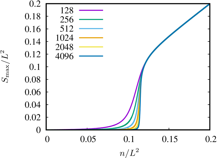
(b)

Figure 2: Examples of dependencies of $S_{\text{max}}/L^{2}$ versus $n/L^{2}$ for various linear system sizes $L=128$, 256, 512, 1024, 2048 and 4096 from top to bottom. (2(a)) sq-7, (2(b)) sq-1,2,3,4,5,6,7

(a)

(b)

Figure 3: Examples of dependencies of $P_{\text{max}}L^{\beta/\nu}$ versus $p$ for various linear system sizes $L=128$, 256, 512, 1024, 2048 and 4096 from top to bottom. (3(a)) sq-7, $p_{c}(\textsc{sq-7})=0.27013$, (3(b)) sq-1,2,3,4,5,6,7, $p_{c}(\textsc{sq-1,2,3,4,5,6,7})=0.11535$

(a)

(b)

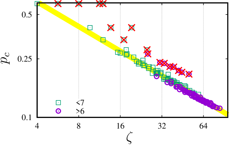
(c)

Figure 4: Dependencies of $p_{c}$ on (4(a)) the total ($z$) and (4(b)) effective ($\zeta$) coordination number for neighborhoods presented in Figure˜1. (4(c)) $p_{c}(\zeta)$ with additional data also for neighborhoods (marked by $\square$) containing sites up to the 6th coordination zone (after Reference [71] and references therein). The inflated neighborhoods (marked by $\times$) are excluded from the fitting procedure. The least-squares fit gives exponent $w\approx 0.5552(42)$

Table 1: Percolation thresholds $p_{c}$ for a square lattice with complex neighborhoods (and their characteristics $z$, $\zeta$) containing sites from the 7th coordination zone presented in Figure˜1

lattice	z	ζ	p_c
lattice	z	ζ	p_c
sq-1,2,3,4,5,6,7	$36$	$84.157$	$0.11535$
sq-2,3,4,5,6,7	$32$	$80.157$	$0.11636$
sq-1,3,4,5,6,7	$32$	$78.500$	$0.11719$
sq-1,2,4,5,6,7	$32$	$76.157$	$0.11949$
sq-1,2,3,5,6,7	$28$	$66.269$	$0.12725$
sq-1,2,3,4,6,7	$32$	$72.844$	$0.12358$
sq-1,2,3,4,5,7	$32$	$72.157$	$0.12562$
sq-3,4,5,6,7	$28$	$74.500$	$0.11859$
sq-2,4,5,6,7	$28$	$72.157$	$0.12132$
sq-2,3,5,6,7	$24$	$62.269$	$0.13241$
sq-2,3,4,6,7	$28$	$68.844$	$0.12488$
sq-2,3,4,5,7	$28$	$68.157$	$0.12770$
sq-1,4,5,6,7	$28$	$70.500$	$0.12236$
sq-1,3,5,6,7	$24$	$60.612$	$0.13112$
sq-1,3,4,6,7	$28$	$67.187$	$0.12644$
sq-1,3,4,5,7	$28$	$66.500$	$0.12830$
sq-1,2,5,6,7	$24$	$58.269$	$0.13339$
sq-1,2,4,6,7	$28$	$64.844$	$0.12864$
sq-1,2,4,5,7	$28$	$64.157$	$0.13089$
sq-1,2,3,6,7	$24$	$54.955$	$0.13973$
sq-1,2,3,5,7	$24$	$54.269$	$0.14470$
sq-1,2,3,4,7	$28$	$60.844$	$0.13718$
sq-4,5,6,7	$24$	$66.500$	$0.12513$
sq-3,5,6,7	$20$	$56.612$	$0.13689$
sq-3,4,6,7	$24$	$63.187$	$0.12848$
sq-3,4,5,7	$24$	$62.500$	$0.13121$
sq-2,5,6,7	$20$	$54.269$	$0.13959$
sq-2,4,6,7	$24$	$60.844$	$0.13104$
sq-2,4,5,7	$24$	$60.157$	$0.13386$
sq-2,3,6,7	$20$	$50.955$	$0.14523$
sq-2,3,5,7	$20$	$50.269$	$0.19672$
sq-2,3,4,7	$24$	$56.844$	$0.14015$
sq-1,5,6,7	$20$	$52.612$	$0.13998$
sq-1,4,6,7	$24$	$59.187$	$0.13298$
sq-1,4,5,7	$24$	$58.500$	$0.13515$
sq-1,3,6,7	$20$	$49.298$	$0.14760$
sq-1,3,5,7	$20$	$48.612$	$0.14876$
sq-1,3,4,7	$24$	$55.187$	$0.14187$
sq-1,2,6,7	$20$	$46.955$	$0.14814$
sq-1,2,5,7	$20$	$46.269$	$0.15298$
sq-1,2,4,7	$24$	$52.844$	$0.14423$
sq-1,2,3,7	$20$	$42.955$	$0.16125$
sq-5,6,7	$16$	$48.612$	$0.14848$
sq-4,6,7	$20$	$55.187$	$0.13708$
sq-4,5,7	$20$	$54.500$	$0.14008$
sq-3,6,7	$16$	$45.298$	$0.15503$
sq-3,5,7	$16$	$44.612$	$0.20250$
sq-3,4,7	$20$	$51.187$	$0.14709$
sq-2,6,7	$16$	$42.955$	$0.15461$
sq-2,5,7	$16$	$42.269$	$0.20831$
sq-2,4,7	$20$	$48.844$	$0.14868$
sq-2,3,7	$16$	$38.955$	$0.21963$
sq-1,6,7	$16$	$41.298$	$0.16193$
sq-1,5,7	$16$	$40.612$	$0.16095$
sq-1,4,7	$20$	$47.187$	$0.15157$
sq-1,3,7	$16$	$37.298$	$0.16973$
sq-1,2,7	$16$	$34.955$	$0.17278$
sq-6,7	$12$	$37.298$	$0.17497$
sq-5,7	$12$	$36.612$	$0.22190$
sq-4,7	$16$	$43.187$	$0.16171$
sq-3,7	$12$	$33.298$	$0.23288$
sq-2,7	$12$	$30.955$	$0.23619$
sq-1,7	$12$	$29.298$	$0.18976$
sq-7	$8$	$25.298$	$0.27013$

IV Discussion

In this paper, the estimation of $p_{c}$ for random site percolation on the square lattice for neighborhoods containing sites from the 7th coordination zone is presented. Monte Carlo simulation with $R=10^{5}$ system realizations for the system sizes from $128^{2}$ to $4096^{2}$ sites allowed us to estimate the percolation thresholds to the $10^{-5}$ accuracy.

The obtained percolation thresholds range from $0.27013$ (for the neighborhood that contains solely sites from the 7th coordination zone) to $0.11535$ (for the neighborhood that contains all sites from the 1st to the 7th coordination zone). The latter agrees perfectly (with the accuracy obtained here, that is $10^{-5}$) with the earlier results of the extensive Monte Carlo simulation (with $L=16384$ and $R>3\cdot 10^{8}$ independent samples produced for each lattice) where $p_{c}(\textsc{sq-1,2,3,4,5,6,7})\approx 0.1153481(9)$ [72].

Capturing the intersection of the rescaled probabilities of belonging to the largest cluster $L^{\beta/\nu}\cdot P_{\text{max}}(p)$ numerically for finite systems is quite challenging as the curves for various $L$ rather seldom intersect exactly at one point (as predicted theoretically by Equation˜2). Also in our case, in Figure˜3, we do not have the intersection of the $L^{\beta/\nu}\cdot P_{\text{max}}(p)$ curves for different $L$ occurring at one point, but rather we can easily identify the value of $p^{*}$ for which the mutual squared differences

$$\delta^{2}(p)=\sum_{i,j}\left[L_{i}^{\beta/\nu}\cdot P_{\text{max}}(p;L_{i})-L_{j}^{\beta/\nu}\cdot P_{\text{max}}(p;L_{j})\right]^{2}$$

between the $L^{\beta/\nu}\cdot P_{\text{max}}(p)$ values—for all studied $L$—is the smallest. This value of $p^{*}$ for which the mutual squared differences $\delta^{2}(p)$ reaches its minimum estimates the percolation threshold $p_{c}\approx p^{*}$ [88]. The convolution (4) can be performed for any arbitrary value of $p$, but the secret of achieving such a small $\delta^{2}$ value that one has the impression it tends to zero lies in the reasonable assumption of the separation $\Delta p$ with which we scan $p$ values. In Figure˜5 we show examples of $L^{\beta/\nu}\cdot P_{\text{max}}(p)$ for $\Delta p=10^{-4}$, $10^{-5}$ and $10^{-6}$. As can be seen, these dependencies allow us to easily indicate the “intersection point” for $\Delta p=10^{-4}$ (Figure˜5(a)) and $10^{-5}$ (Figure˜5(b)). That is, just by inspection, even without calculating $\delta^{2}$, one can see a higher dispersion of the values $L^{\beta/\nu}\cdot P_{\text{max}}(p)$ for the considered values of $L$ and thus larger $\delta^{2}(p)$ at points $p=(p^{*}-\Delta p)$ and $p=(p^{*}+\Delta p)$ than at $p=p^{*}$. This means that the true value of $p_{c}$ is somewhere inside the interval $(p^{*}-\Delta p,p^{*}+\Delta p)$.

On the other hand, for $\Delta p=10^{-6}$ (see Figure˜5(c)) we cannot easily identify the “intersection point”. The reason for this lies in too weak statistics, i.e., too small number $R$ of the simulation repetition. The precision of determining the value of $P_{\text{max}}(n)$—i.e. $\bar{X}(n;N)$ in Equation˜4–is $1/R$ and affects the selection of $\Delta p$ value, which allows observing a clear $\delta^{2}(p)$ minimum for $p=p^{*}$, with a simultaneous clear spread of points $L^{\beta/\nu}\cdot P_{\text{max}}(p)$ for various $L$ at $p=p^{*}-\Delta p$ and $p=p^{*}+\Delta p$. Hence, we consider $\Delta p=10^{-5}$ as the uncertainty of the determined $p_{c}$. Moreover, plotting $L^{\beta/\nu}\cdot P_{\text{max}}(p)$ for finite $L$ according to Equation˜1 allows us to eliminate, at least partially, the effect of finite sizes on the accuracy of determining $p_{c}$.

In Figure˜4(b) we clearly observe two series of data, roughly for $p_{c}$ below and above 0.2. The latter correspond to sq-7, sq-2,7, sq-3,7, sq-5,7, sq-2,3,7, sq-2,5,7, sq-3,5,7 and sq-2,3,5,7. These neighborhoods are the so-called inflated neighborhoods, which means that they have partners with lower indexed neighborhoods with the same $p_{c}$ and $z$. These partners are presented in Figure˜6.

Similarly to neighborhoods with smaller ranges, the power-law dependence of the percolation threshold on the effective coordination number with exponent $w$ close to $-1/2$ is observed. The power law is obtained after excluding $p_{c}$ of the inflated neighborhoods (marked by $\times$ in Figure˜4(c)) from the fitting procedure.

Introducing the effective coordination number $\zeta$ partially eliminates the degeneration (see Figure˜4(b)) strongly observed in the dependence on $p_{c}(z)$ (see Figure˜4(a)). For $p_{c}(\zeta)$, we still observe this degeneration in several cases, such as

• $\zeta(\textsc{sq-1,3,7})=\zeta(\textsc{sq-6,7})$,

• $\zeta(\textsc{sq-1,2,3,7})=\zeta(\textsc{sq-2,6,7})$,

• $\zeta(\textsc{sq-1,3,5,7})=\zeta(\textsc{sq-5,6,7})$,

• $\zeta(\textsc{sq-1,3,4,7})=\zeta(\textsc{sq-4,6,7})$,

• $\zeta(\textsc{sq-1,2,3,4,7})=\zeta(\textsc{sq-2,4,6,7})$,

• $\zeta(\textsc{sq-1,3,4,5,7})=\zeta(\textsc{sq-4,5,6,7})$,

• $\zeta(\textsc{sq-1,2,3,4,5,7})=\zeta(\textsc{sq-2,4,5,6,7})$.

This degeneration in distinguishing neighborhoods based only on the scalar variable can be resolved after normalization of $\zeta$ to the total number of sites in the neighborhood $z$. The fraction $\zeta/z$ is nothing else but the mean distance

$$\bar{r}=\frac{1}{z}\sum_{i}z_{i}r_{i}$$ (8)

of sites in the neighborhood to the central site. We can call it the mean radius of the neighborhood.

(a)

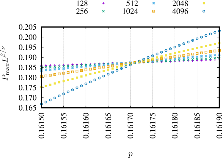
(b)

(c)

Figure 5: Dependencies $L^{\beta/\nu}\cdot P_{\text{max}}(p)$ for various values of the separation $\Delta p$: (5(a)) $10^{-4}$, (5(b)) $10^{-5}$, (5(c)) $10^{-6}$. With assumed number of repetition of simulations ($R=10^{5}$) value $\Delta p=10^{-6}$ is insufficient to see clear “single crossing-point” and to identify $p=p^{*}$

(a)

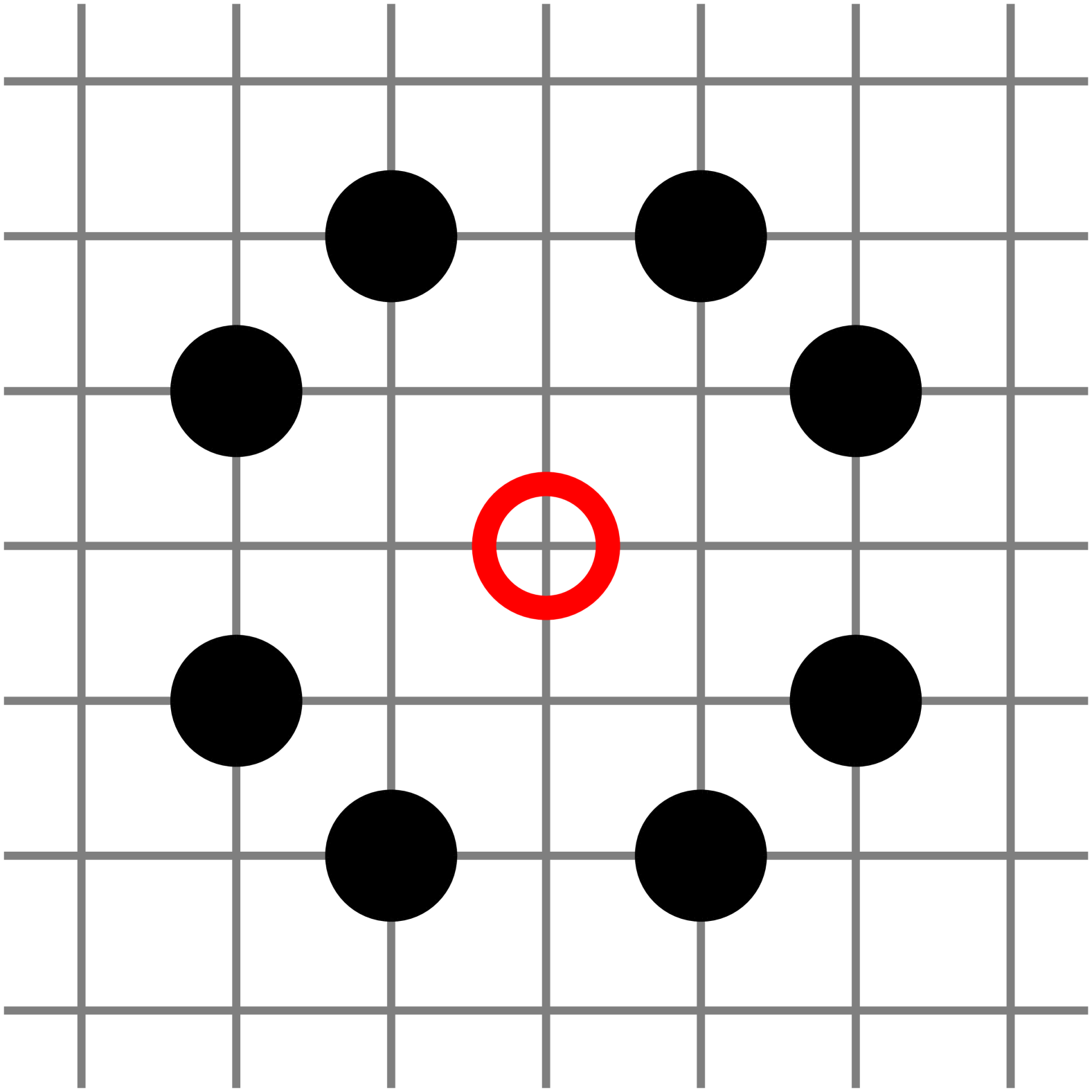
(b)

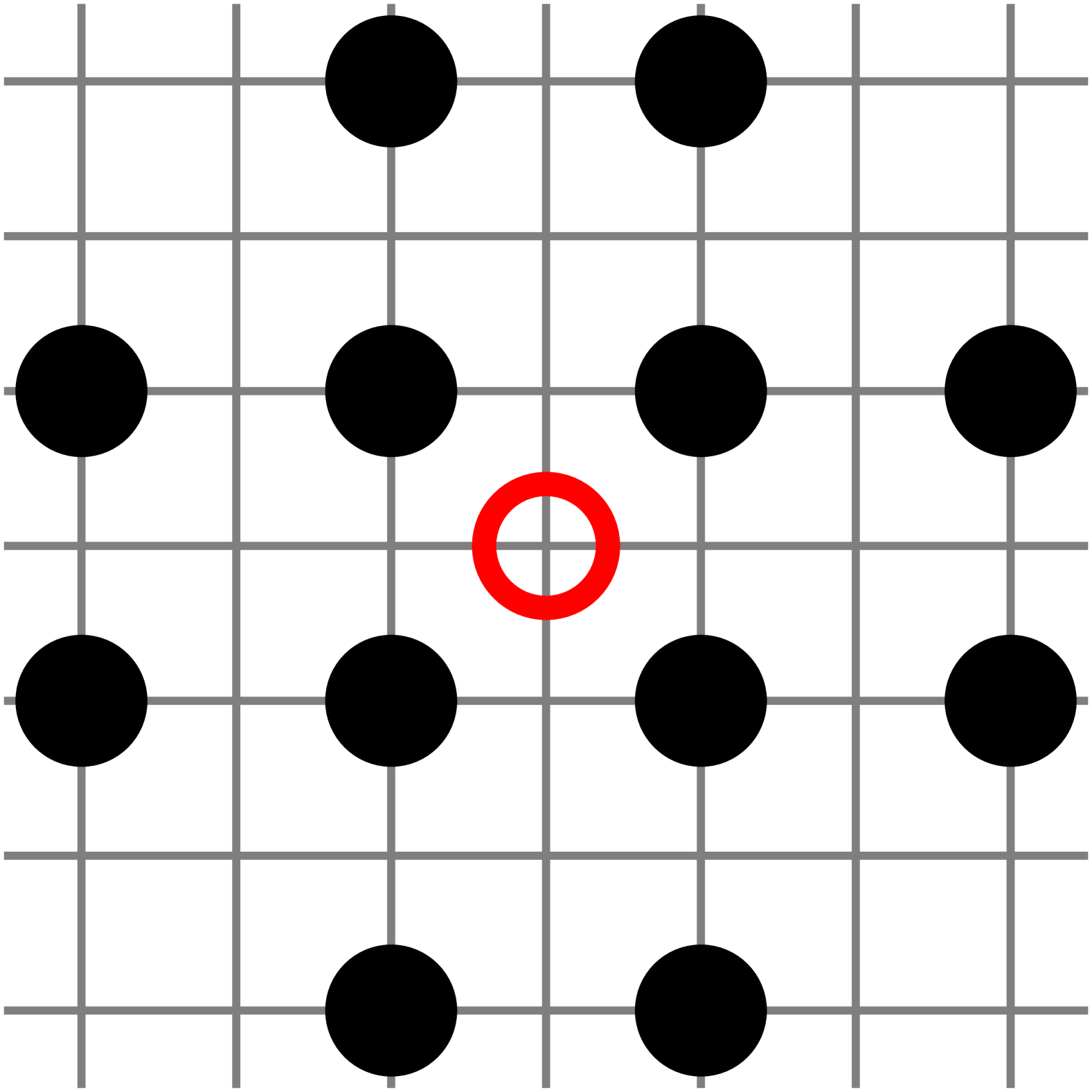
(c)

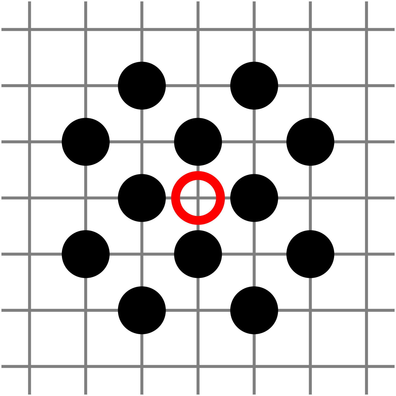
(d)

(e)

(f)

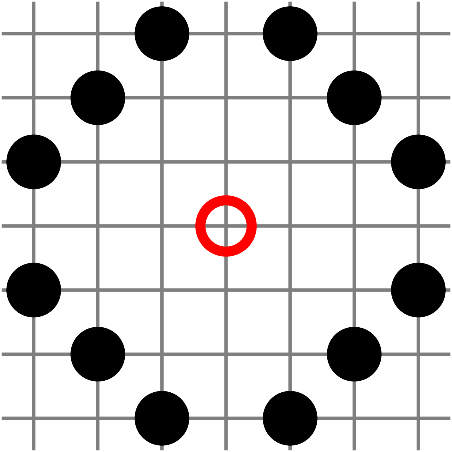
(g)

(h)

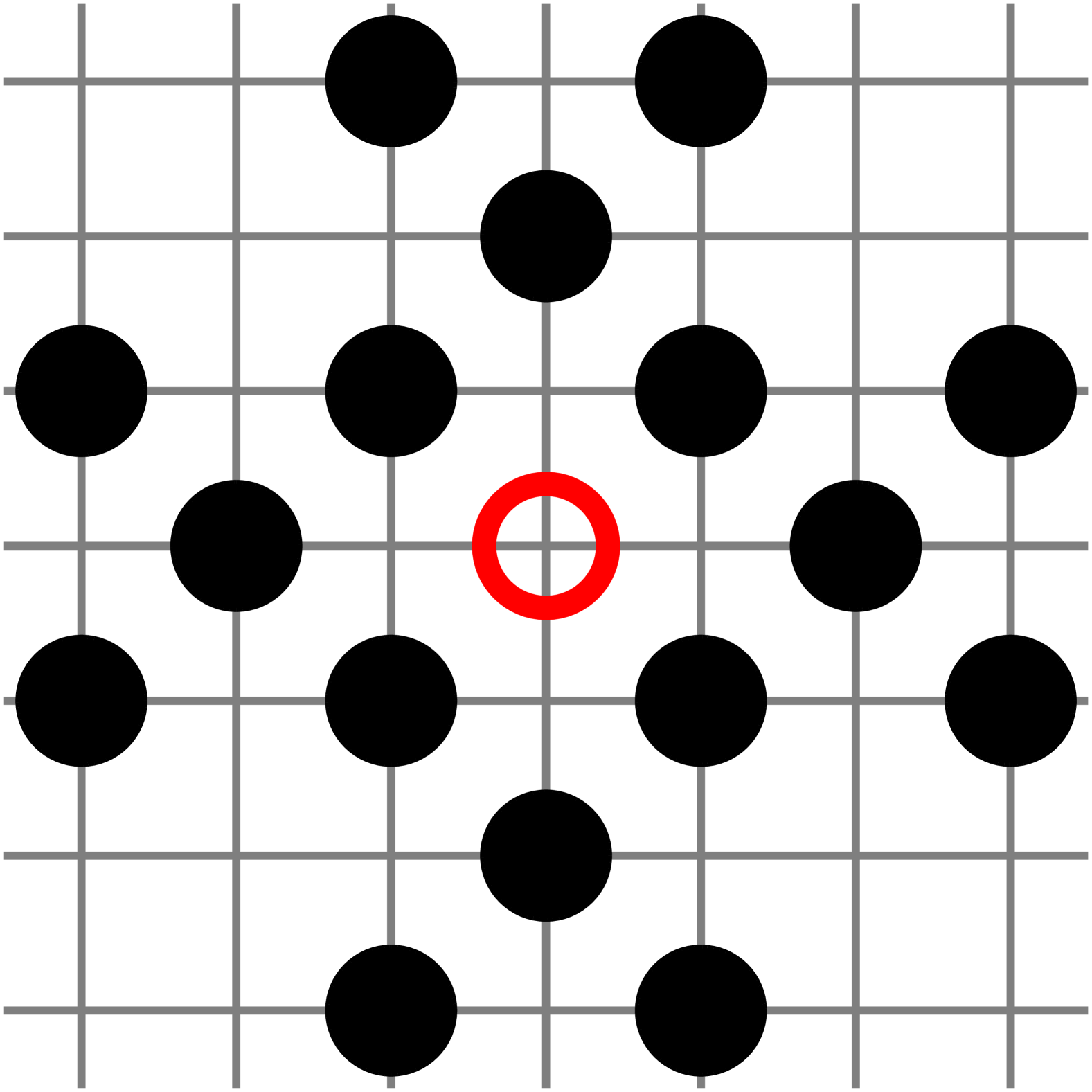
(i)

(j)

(k)

(l)

(m)

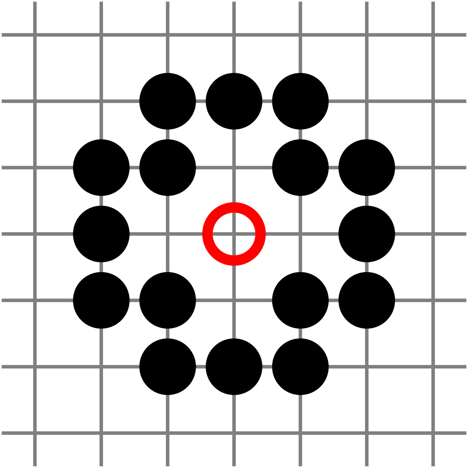
(n)

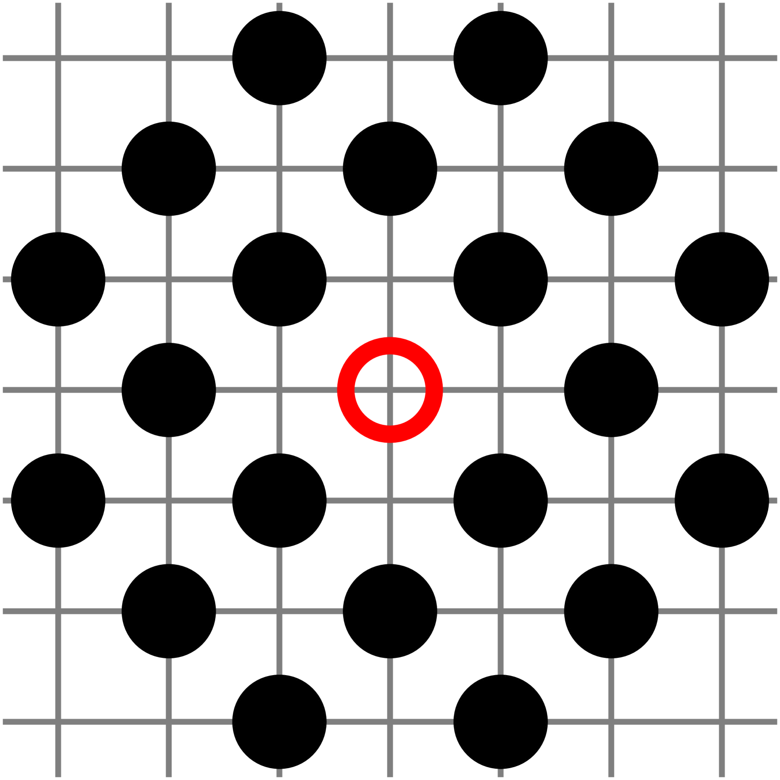
(o)

(p)

Figure 6: Inflated neighborhoods (6(a)) sq-7, (6(c)) sq-2,7, (6(e)) sq-3,7, (6(g)) sq-5,7, (6(i)) sq-2,3,7, (6(k)) sq-2,5,7, (6(m)) sq-3,5,7, (6(o)) sq-2,3,5,7 and their lower indexed partners (6(b)) sq-4, (6(d)) sq-1,4, (6(f)) sq-2,4, (6(h)) sq-3,4, (6(j)) sq-1,2,4, (6(l)) sq-1,3,4, (6(n)) sq-2,3,4, (6(p)) sq-1,2,3,4

In Figure˜7 we show the dependence $p_{c}$ on the mean radius $\bar{r}$ for the 131 neighborhoods that contain sites in the range smaller than or equal to $\bar{r}(\textsc{sq-7})=\sqrt{10}$. In this plot, only three neighborhoods have identical mean radius $\bar{r}(\textsc{sq-3})=\bar{r}(\textsc{sq-1,6})=\bar{r}(\textsc{sq-1,3,6})=2$ (these three neighborhoods are marked by $\times$). Furthermore, we can empirically determine the lower limit of the percolation threshold for complex neighborhoods as

$$p_{c}(\textsc{sq})\geq\frac{p_{c}(\textsc{sq-1})}{\bar{r}^{2}}.$$ (9)

This limit also holds for extended neighborhoods with sites beyond the 7th coordination zone, for example sq-1,2,3,4,5,6,7,8, sq-1,2,3,4,5,6,7,8,9 and sq-1,2,3,4,5,6,7,8,9,10 ($p_{c}$ values for these neighborhoods are taken after Reference [73]). The results for extended neighborhoods (which are both complex and compact, marked by $+$ in Figure˜7) touch the boundary line of inequality (9).

Figure 7: Dependence of percolation threshold $p_{c}$ on mean radius $\bar{r}$ of the neighborhoods. The mean radius $\bar{r}$ uniquely identifies neighborhoods except of three neighborhoods sq-3, sq-1,6 and sq-1,3,6 all with mean radius equal to two. These three neighborhoods are marked by crosses ($\times$). The open squares ($\square$) correspond to sq-1,2,3,4,5,6,7,8, sq-1,2,3,4,5,6,7,8,9, sq-1,2,3,4,5,6,7,8,9,10 neighborhoods (after Reference [73]). Pluses ($+$) show $p_{c}$ associated with compact neighborhoods

Also in Reference [73]—from which we took values of $p_{c}$ for sq-1,2,3,4,5,6,7,8, sq-1,2,3,4,5,6,7,8,9, sq-1,2,3,4,5,6,7,8,9,10 neighborhoods—Xun et al. studied, among other things, also the percolation thresholds for regular lattices with compact extended-range neighborhoods in two dimensions. For all Archimedean lattices and up to the 10th nearest neighbors, they show the dependence $z$ versus $1/p_{c}$ (Figure 7 in Reference [73]) and $-1/\ln(1-p_{c})$ (Figure 8 in Reference [73]). For new variables $y=z$ and $x=1/p_{c}$ or $x=-1/\ln(1-p_{c})$ in both cases the slope of the straight line close to the experimental points is $y=4.521x$ and the value of $4.521=4\eta_{c}$ comes from the critical filling factor of circular neighborhoods in two dimensions (i.e. for continuous percolation of discs, where $\eta_{c}=1.12808737(6)$ [89]). The experimental data for $z$ vs. $1/p_{c}$ lie below this straight line as compact neighborhoods become solid discs in the limit of $z\to\infty$. In Figure˜8 the reciprocal of $p_{c}$ both from our work (against $r^{2}$) and the continuous percolation limit (from Reference [73], against $z$) are presented. As we can see, for compact neighborhoods (at least for the square lattice and site percolation problem), we can confine percolation thresholds $p_{c}$ between two curves.

To conclude, we calculated 64 percolation thresholds for neighborhoods containing sites from the 7th coordination zone, of which 63 are evaluated for the first time. The obtained values of $p_{c}$ follow the early prediction of $p_{c}(\zeta)$, which is given by the power law $p_{c}\propto\zeta^{-w}$ with the exponent $w$ close to $1/2$. Investigating the degeneration of $p_{c}$ versus $\zeta$ allowed us to determine the lower limit $p_{c}$ as dependent on the inverse square of the mean distance $\bar{r}$ of sites in the neighborhoods. The latter touches the boundary line for the extended (compact) neighborhoods. These results enrich earlier studies of site percolation for compact neighborhoods [73] where $p_{c}$ values were restricted by the limitation predicted by $1/p_{c}>z/(4\eta_{c})$, where $\eta_{c}$ is the critical filling factor for the continuous percolation of discs. Finally, we also recalculated $p_{c}(\textsc{sq-2,4})=0.23288$, which means that its value provided in Reference [77] as $p_{c}(\textsc{sq-2,4})=0.225$ was clearly underestimated.

Figure 8: Dependence of reciprocal percolation threshold $1/p_{c}$ on $\bar{r}^{2}$ and $z$ of the neighborhoods. Data for sq-1,2,3,4,5,6,7,8, sq-1,2,3,4,5,6,7,8,9, sq-1,2,3,4,5,6,7,8,9,10 neighborhoods are taken from Reference [73] together with the continuous percolation limit of the discs ($4\eta_{c}$)

Further studies may concentrate on the estimation of the percolation thresholds $p_{c}$ for triangular or honeycomb lattices with complex neighborhoods containing sites from the 7th coordination zone or validation of Equation˜9 for other lattices.

Appendix A

In Listing LABEL:lst:code the boundaries() procedure to be replaced in the original program published in Reference [86] is presented. The example corresponds to the sq-7 neighborhood.

Listing 1: boundaries() procedure for sq-7 neighborhood to be inserted in Newman–Ziff algorithm code published in Reference [86]

⬇

1// SQ-7

2#define L 9 /* Linear dimension */

3#define Z 8

4#define N (L*L)

5

6int nn[N][Z]; /* Nearest neighbors */

7

8void boundaries() {

9 int i,j;

10 for(i=0; i<N; i++) {

11 // 7nn core:

12 nn[i][0] = (N+i +L+3)%N;

13 nn[i][1] = (N+i +L-3)%N;

14 nn[i][2] = (N+i -L+3)%N;

15 nn[i][3] = (N+i -L-3)%N;

16 nn[i][4] = (N+i +3*L+1)%N;

17 nn[i][5] = (N+i +3*L-1)%N;

18 nn[i][6] = (N+i -3*L+1)%N;

19 nn[i][7] = (N+i -3*L-1)%N;

20 // 7nn left border:

21 if(i%L==0) {

22 nn[i][1] = (N+L+i +L-3)%N;

23 nn[i][3] = (N+L+i -L-3)%N;

24 nn[i][5] = (N+L+i +3*L-1)%N;

25 nn[i][7] = (N+L+i -3*L-1)%N; }

26 if(i%L==1 || i%L==2) {

27 nn[i][1] = (N+L+i +L-3)%N;

28 nn[i][3] = (N+L+i -L-3)%N; }

29 // 7nn right border:

30 if((i+3)%L==0 || (i+2)%L==0) {

31 nn[i][0] = (N-L+i +L+3)%N;

32 nn[i][2] = (N-L+i -L+3)%N; }

33 if((i+1)%L==0) {

34 nn[i][0] = (N-L+i +L+3)%N;

35 nn[i][2] = (N-L+i -L+3)%N;

36 nn[i][4] = (N-L+i +3*L+1)%N;

37 nn[i][6] = (N-L+i -3*L+1)%N; }

38 }

39}

References

- Stauffer and Aharony [1994] D. Stauffer and A. Aharony, Introduction to Percolation Theory, 2nd ed. (Taylor and Francis, London, 1994).
- Bollobás and Riordan [2006] B. Bollobás and O. Riordan, Percolation (Cambridge UP, Cambridge, 2006).
- Sahimi [1994] M. Sahimi, Applications of Percolation Theory (Taylor and Francis, London, 1994).
- Kesten [1982] H. Kesten, Percolation Theory for Mathematicians (Brikhauser, Boston, 1982).
- Saberi [2015] A. A. Saberi, Recent advances in percolation theory and its applications, Physics Reports 578, 1 (2015).
- Li et al. [2021] M. Li, R.-R. Liu, L. Lü, M.-B. Hu, S. Xu, and Y.-C. Zhang, Percolation on complex networks: Theory and application, Physics Reports 907, 1 (2021).
- Sykes and Essam [1964a] M. F. Sykes and J. W. Essam, Exact critical percolation probabilities for site and bond problems in two dimensions, Journal of Mathematical Physics 5, 1117 (1964a).
- Ziff and Scullard [2006] R. M. Ziff and C. R. Scullard, Exact bond percolation thresholds in two dimensions, Journal of Physics A: Mathematical and General 39, 15083 (2006).
- Scullard [2006] C. R. Scullard, Exact site percolation thresholds using a site-to-bond transformation and the star-triangle transformation, Physical Review E 73, 016107 (2006).
- Jacobsen [2014] J. L. Jacobsen, High-precision percolation thresholds and Potts-model critical manifolds from graph polynomials, Journal of Physics A: Mathematical and Theoretical 47, 135001 (2014).
- Coupette and Schilling [2022] F. Coupette and T. Schilling, Exactly solvable percolation problems, Physical Review E 105, 044108 (2022).
- Akhunzhanov et al. [2022] R. K. Akhunzhanov, A. V. Eserkepov, and Y. Y. Tarasevich, Exact percolation probabilities for a square lattice: Site percolation on a plane, cylinder, and torus, Journal of Physics A: Mathematical and Theoretical 55, 204004 (2022).
- Broadbent and Hammersley [1957] S. R. Broadbent and J. M. Hammersley, Percolation processes: I. Crystals and mazes, Mathematical Proceedings of the Cambridge Philosophical Society 53, 629 (1957).
- Hammersley [1957] J. M. Hammersley, Percolation processes: II. The connective constant, Mathematical Proceedings of the Cambridge Philosophical Society 53, 642 (1957).
- Soto-Gomez et al. [2020] D. Soto-Gomez, L. Vazquez Juiz, P. Perez-Rodriguez, J. Eugenio Lopez-Periago, M. Paradelo, and J. Koestel, Percolation theory applied to soil tomography, Geoderma 357, 113959 (2020).
- Bolandtaba and Skauge [2011] S. F. Bolandtaba and A. Skauge, Network modeling of eor processes: A combined invasion percolation and dynamic model for mobilization of trapped oil, Transport in Porous Media 89, 357 (2011).
- Mun et al. [2014] S. C. Mun, M. Kim, K. Prakashan, H. J. Jung, Y. Son, and O. O. Park, A new approach to determine rheological percolation of carbon nanotubes in microstructured polymer matrices, Carbon 67, 64 (2014).
- Ghanbarian et al. [2020] B. Ghanbarian, F. Liang, and H.-H. Liu, Modeling gas relative permeability in shales and tight porous rocks, Fuel 272, 117686 (2020).
- Ueland et al. [2018] B. G. Ueland, N. H. Jo, A. Sapkota, W. Tian, M. Masters, H. Hodovanets, S. S. Downing, C. Schmidt, R. J. McQueeney, S. L. Bud’ko, A. Kreyssig, P. C. Canfield, and A. I. Goldman, Reduction of the ordered magnetic moment and its relationship to Kondo coherence in Ce1-xLaxCu2Ge2, Physical Review B 97, 165121 (2018).
- Keeney et al. [2017] L. Keeney, C. Downing, M. Schmidt, M. E. Pemble, V. Nicolosi, and R. W. Whatmore, Direct atomic scale determination of magnetic ion partition in a room temperature multiferroic material, Scientific Reports 7, 1737 (2017).
- Buczek et al. [2016] P. Buczek, L. M. Sandratskii, N. Buczek, S. Thomas, G. Vignale, and A. Ernst, Magnons in disordered nonstoichiometric low-dimensional magnets, Physical Review B 94, 054407 (2016).
- Yiu et al. [2014] Y. Yiu, P. Bonfá, S. Sanna, R. De Renzi, P. Carretta, M. A. McGuire, A. Huq, and S. E. Nagler, Tuning the magnetic and structural phase transitions of PrFeAsO via Fe/Ru spin dilution, Physical Review B 90, 064515 (2014).
- Grady [2023] M. Grady, Possible new phase transition in the 3D Ising model associated with boundary percolation, Journal of Physics: Condensed Matter 35, 285401 (2023).
- Jeong et al. [2018] J. Jeong, K. J. Park, E.-J. Cho, H.-J. Noh, S. B. Kim, and H.-D. Kim, Electronic structure change of NiS2-xSex in the metal-insulator transition probed by X-ray absorption spectroscopy, Journal of the Korean Physical Society 72, 111 (2018).
- Avella et al. [2019] A. Avella, A. M. Oles, and P. Horsch, Defect-induced orbital polarization and collapse of orbital order in doped vanadium perovskites, Physical Review Letters 122, 127206 (2019).
- Cheng et al. [2020] L. Cheng, P. Yan, X. Yang, H. Zou, H. Yang, and H. Liang, High conductivity, percolation behavior and dielectric relaxation of hybrid ZIF-8/CNT composites, Journal of Alloys and Compounds 825, 154132 (2020).
- Xu et al. [2014] F. Xu, Z. Xu, and B. I. Yakobson, Site-percolation threshold of carbon nanotube fibers—Fast inspection of percolation with Markov stochastic theory, Physica A 407, 341 (2014).
- Sykes and Glen [1976] M. Sykes and M. Glen, Percolation processes in 2 dimensions. 1. Low-density series expansions, Journal of Physics A: Mathematical & General 9, 87 (1976).
- Sykes et al. [1976a] M. Sykes, D. Gaunt, and M. Glen, Percolation processes in 2 dimensions. 2. Critical concentrations and mean size index, Journal of Physics A: Mathematical & General 9, 97 (1976a).
- Sykes et al. [1976b] M. Sykes, D. Gaunt, and M. Glen, Percolation processes in 2 dimensions. 3. High-density series expansions, Journal of Physics A: Mathematical & General 9, 715 (1976b).
- Sykes et al. [1976c] M. Sykes, D. Gaunt, and M. Glen, Percolation processes in 2 dimensions. 4. Percolation probability, Journal of Physics A: Mathematical & General 9, 725 (1976c).
- Gaunt and Sykes [1976] D. Gaunt and M. Sykes, Percolation processes in 2 dimensions. 5. Exponent and scaling theory, Journal of Physics A: Mathematical & General 9, 1109 (1976).
- Meyers [2007] L. A. Meyers, Contact network epidemiology: Bond percolation applied to infectious disease prediction and control, Bulletin of the American Mathematical Society 44, 63 (2007).
- Lee and Zhu [2021] D.-S. Lee and M. Zhu, Epidemic spreading in a social network with facial masks wearing individuals, IEEE Transactions on Computational Social Systems 8, 1393 (2021).
- Ziff [2021] R. M. Ziff, Percolation and the pandemic, Physica A 568, 125723 (2021).
- Malarz et al. [2002] K. Malarz, S. Kaczanowska, and K. Kułakowski, Are forest fires predictable?, International Journal of Modern Physics C 13, 1017 (2002).
- Guisoni et al. [2011] N. Guisoni, E. S. Loscar, and E. V. Albano, Phase diagram and critical behavior of a forest-fire model in a gradient of immunity, Physical Review E 83, 011125 (2011).
- Simeoni et al. [2011] A. Simeoni, P. Salinesi, and F. Morandini, Physical modelling of forest fire spreading through heterogeneous fuel beds, International Journal of Wildland Fire 20, 625 (2011).
- Camelo-Neto and Coutinho [2011] G. Camelo-Neto and S. Coutinho, Forest-fire model with resistant trees, Journal of Statistical Mechanics—Theory and Experiments 2011, P06018 (2011).
- Abades et al. [2014] S. R. Abades, A. Gaxiola, and P. A. Marquet, Fire, percolation thresholds and the savanna forest transition: A neutral model approach, Journal of Ecology 102, 1386 (2014).
- Ramírez et al. [2020] J. E. Ramírez, C. Pajares, M. I. Martínez, R. Rodríguez Fernández, E. Molina-Gayosso, J. Lozada-Lechuga, and A. Fernández Téllez, Site-bond percolation solution to preventing the propagation of Phytophthora zoospores on plantations, Physical Review E 101, 032301 (2020).
- Rosales Herrera et al. [2021] D. Rosales Herrera, J. E. Ramírez, M. I. Martínez, H. Cruz-Suárez, A. Fernández Téllez, J. F. López-Olguín, and A. Aragón García, Percolation-intercropping strategies to prevent dissemination of phytopathogens on plantations, Chaos 31, 063105 (2021).
- Herrera et al. [2024] D. R. Herrera, J. Velázquez-Castro, A. F. Téllez, J. F. López-Olguín, and J. E. Ramírez, Site percolation threshold of composite square lattices and its agroecology applications, Physical Review E 109, 014304 (2024).
- Cao et al. [2020] W. Cao, L. Dong, L. Wu, and Y. Liu, Quantifying urban areas with multi-source data based on percolation theory, Remote Sensing of Environment 241, 111730 (2020).
- Ng et al. [2024] M. K. M. Ng, Z. Shabrina, S. Sarkar, H. Han, and C. Pettit, From urban clusters to megaregions: mapping Australia’s evolving urban regions, Computational Urban Science 4, 28 (2024).
- Alguero et al. [2020] M. Alguero, M. Perez-Cerdan, R. P. del Real, J. Ricote, and A. Castro, Novel Aurivillius Bi4Ti3-2xNbxFexO12 phases with increasing magnetic-cation fraction until percolation: A novel approach for room temperature multiferroism, Journal of Materials Chemistry C 8, 12457 (2020).
- Moreira et al. [2001] A. Moreira, J. Andrade, and D. Stauffer, Sznajd social model on square lattice with correlated percolation, International Journal of Modern Physics C 12, 39 (2001).
- Malarz and Wołoszyn [2023] K. Malarz and M. Wołoszyn, Thermal properties of structurally balanced systems on classical random graphs, Chaos 33, 073115 (2023).
- Cirigliano et al. [2023] L. Cirigliano, C. Castellano, and G. Timár, Extended-range percolation in complex networks, Physical Review E 108, 044304 (2023).
- Bartolucci et al. [2020] S. Bartolucci, F. Caccioli, and P. Vivo, A percolation model for the emergence of the Bitcoin Lightning Network, Scientific Reports 10, 4488 (2020).
- Beddoe et al. [2023] M. Beddoe, T. Gölz, M. Barkey, E. Bau, M. Godejohann, S. A. Maier, F. Keilmann, M. Moldovan, D. Prodan, N. Ilie, and A. Tittl, Probing the micro- and nanoscopic properties of dental materials using infrared spectroscopy: A proof-of-principle study, Acta Biomaterialia 168, 309 (2023).
- Grassberger [2003] P. Grassberger, Critical percolation in high dimensions, Physical Review E 67, 036101 (2003).
- Sykes and Essam [1964b] M. F. Sykes and J. W. Essam, Critical percolation probabilities by series methods, Physical Review 133, A310 (1964b).
- Sur et al. [1976] A. Sur, J. L. Lebowitz, J. Marro, M. H. Kalos, and S. Kirkpatrick, Monte carlo studies of percolation phenomena for a simple cubic lattice, Journal of Statistical Physics 15, 345 (1976).
- Gaunt and Sykes [1983] D. Gaunt and M. Sykes, Series study of random percolation in 3 dimensions, Journal of Physics A: Mathematical & General 16, 783 (1983).
- Lorenz and Ziff [1998] C. Lorenz and R. Ziff, Universality of the excess number of clusters and the crossing probability function in three-dimensional percolation, Journal of Physics A: Mathematical & General 31, 8147 (1998).
- Kurzawski and Malarz [2012] Ł. Kurzawski and K. Malarz, Simple cubic random-site percolation thresholds for complex neighbourhoods, Reports on Mathematical Physics 70, 163 (2012).
- Kotwica et al. [2019] M. Kotwica, P. Gronek, and K. Malarz, Efficient space virtualisation for Hoshen–Kopelman algorithm, International Journal of Modern Physics C 30, 1950055 (2019).
- Zhao et al. [2022] P. Zhao, J. Yan, Z. Xun, D. Hao, and R. M. Ziff, Site and bond percolation on four-dimensional simple hypercubic lattices with extended neighborhoods, Journal of Statistical Mechanics: Theory and Experiment 2022, 033202 (2022).
- Paul et al. [2001] G. Paul, R. M. Ziff, and H. E. Stanley, Percolation threshold, Fisher exponent, and shortest path exponent for four and five dimensions, Physical Review E 64, 026115 (2001).
- Xun et al. [2023] Z. Xun, D. Hao, and R. M. Ziff, Extended-range percolation in five dimensions (2023), arXiv:2308.15719 [cond-mat.stat-mech] .
- Van der Marck [1998] S. Van der Marck, Calculation of percolation thresholds in high dimensions for FCC, BCC and diamond lattices, International Journal of Modern Physics C 9, 529 (1998).
- Koza and Poła [2016] Z. Koza and J. Poła, From discrete to continuous percolation in dimensions 3 to 7, Journal of Statistical Mechanics: Theory and Experiment 2016, 103206 (2016).
- Haji-Akbari and Ziff [2009] A. Haji-Akbari and R. M. Ziff, Percolation in networks with voids and bottlenecks, Physical Review E 79, 021118 (2009).
- Mitra et al. [2019] S. Mitra, D. Saha, and A. Sensharma, Percolation in a distorted square lattice, Physical Review E 99, 012117 (2019).
- Mitra et al. [2022] S. Mitra, D. Saha, and A. Sensharma, Percolation in a simple cubic lattice with distortion, Physical Review E 106, 034109 (2022).
- Mitra and Sensharma [2023] S. Mitra and A. Sensharma, Site percolation in distorted square and simple cubic lattices with flexible number of neighbors, Physical Review E 107, 064127 (2023).
- Cruz et al. [2023] M.-A. M. Cruz, J. P. Ortiz, M. P. Ortiz, and A. Balankin, Percolation on fractal networks: A survey, Fractal and Fractional 7, 231 (2023).
- Dalton et al. [1964] N. W. Dalton, C. Domb, and M. F. Sykes, Dependence of critical concentration of a dilute ferromagnet on the range of interaction, Proceedings of the Physical Society 83, 496 (1964).
- Domb and Dalton [1966] C. Domb and N. W. Dalton, Crystal statistics with long-range forces: I. The equivalent neighbour model, Proceedings of the Physical Society 89, 859 (1966).
- Malarz [2024] K. Malarz, Universality of percolation thresholds for two-dimensional complex non-compact neighborhoods, Physical Review E 109, 034108 (2024).
- Xun et al. [2021a] Z. Xun, D. Hao, and R. M. Ziff, Site percolation on square and simple cubic lattices with extended neighborhoods and their continuum limit, Physical Review E 103, 022126 (2021a).
- Xun et al. [2022] Z. Xun, D. Hao, and R. M. Ziff, Site and bond percolation thresholds on regular lattices with compact extended-range neighborhoods in two and three dimensions, Physical Review E 105, 024105 (2022).
- Xun and Hao [2022] Z. Xun and D. Hao, Monte Carlo simulation of bond percolation on square lattice with complex neighborhoods, Acta Physica Sinica 71, 066401 (2022), in Chinese.
- Malarz and Galam [2005] K. Malarz and S. Galam, Square-lattice site percolation at increasing ranges of neighbor bonds, Physical Review E 71, 016125 (2005).
- Galam and Malarz [2005] S. Galam and K. Malarz, Restoring site percolation on damaged square lattices, Physical Review E 72, 027103 (2005).
- Majewski and Malarz [2007] M. Majewski and K. Malarz, Square lattice site percolation thresholds for complex neighbourhoods, Acta Physica Polonica B 38, 2191 (2007).
- Malarz [2015] K. Malarz, Simple cubic random-site percolation thresholds for neighborhoods containing fourth-nearest neighbors, Physical Review E 91, 043301 (2015).
- Malarz [2020] K. Malarz, Site percolation thresholds on triangular lattice with complex neighborhoods, Chaos 30, 123123 (2020).
- Malarz [2021] K. Malarz, Percolation thresholds on triangular lattice for neighbourhoods containing sites up to the fifth coordination zone, Physical Review E 103, 052107 (2021).
- Malarz [2022] K. Malarz, Random site percolation on honeycomb lattices with complex neighborhoods, Chaos 32, 083123 (2022).
- Malarz [2023] K. Malarz, Random site percolation thresholds on square lattice for complex neighborhoods containing sites up to the sixth coordination zone, Physica A 632, 129347 (2023).
- Xun et al. [2021b] Z. Xun, D. Hao, and R. M. Ziff, Site percolation on square and simple cubic lattices with extended neighborhoods and their continuum limit, Physical Review E 103, 022126 (2021b).
- Privman [1990] V. Privman, Finite-size scaling theory, in Finite size scaling and numerical simulation of statistical systems, edited by V. Privman (World Scientific, Singapore, 1990) pp. 1–98.
- Landau and Binder [2009] D. P. Landau and K. Binder, A Guide to Monte Carlo Simulations in Statistical Physics, 3rd ed. (Cambridge University Press, Cambridge, 2009).
- Newman and Ziff [2001] M. E. J. Newman and R. M. Ziff, Fast Monte Carlo algorithm for site or bond percolation, Physical Review E 64, 016706 (2001).
- [87] See Supplemental Material at https://doi.org/10.58032/AGH/SWJZKD for dependencies for all neighborhoods containg sites from the 7th coordination zone.
- Bastas et al. [2014] N. Bastas, K. Kosmidis, P. Giazitzidis, and M. Maragakis, Method for estimating critical exponents in percolation processes with low sampling, Physical Review E 90, 062101 (2014).
- Mertens and Moore [2012] S. Mertens and C. Moore, Continuum percolation thresholds in two dimensions, Physical Review E 86, 061109 (2012).