Leveraging Code Structure to Improve Soft Output for GRAND, GCD, OSD, and SCL

Abstract

In addition to a proposed codeword, error correction decoders that provide blockwise soft output (SO) return an estimate of the likelihood that the decoding is correct. Following Forney, such estimates are traditionally only possible for list decoders where the soft output is the likelihood that a decoding is correct given it is assumed to be in the list. Recently, it has been established that Guessing Random Additive Noise Decoding (GRAND), Guessing Codeword Decoding (GCD), Ordered Statistics Decoding (OSD), and Successive Cancellation List (SCL) decoding can provide more accurate soft output, even without list decoding. Central to the improvement is a per-decoding estimate of the likelihood that a decoding has not been found that can be readily calculated during the decoding process. Here we explore how linear codebook constraints can be employed to further enhance the precision of such SO. We evaluate performance by adapting a forecasting statistic called the Brier Score. Results indicate that the SO generated by the approach is essentially as accurate as the maximum a posteriori estimate.

I Introduction

For any soft input (SI) error correction decoder, it would be desirable if, in addition to a codeword, it returned blockwise soft output (SO) in the form of an accurate a posteriori likelihood that the proposed decoding is correct. Blockwise SO could be leveraged to decide whether retransmission is necessary, or to calculate bitwise SO and so enable iterative decoding of long, powerful codes. The first blockwise SO formula was established by Forney [1]. It necessitates a list decoder as the SO is approximated by the conditional probability that each codeword in a list is correct given the transmitted codeword is assumed to be in the list. The same approximation underlies the celebrated Chase-Pyndiah iterative SISO decoder of turbo product codes [2] and subsequent alternatives [3, 4, 5, 6, 7].

Recently, it was established that SI Guessing Random Additive Noise Decoding (GRAND) algorithms [8, 9, 10, 11, 12] can produce accurate blockwise SO, even for a single decoding [13, 14]. The key advance is the derivation of an estimate of the likelihood that the correct decoding has not been yet found that can be readily evaluated during decoding, which removes Forney’s conditioning. That feature enables SO without list decoding while also improving SO for list decoding. Adapting the derivation of that estimate for GRAND, it has since been shown that accurate blockwise SO can also be extracted from Guessing Codeword Decoding (GCD) [15, 16] or any version of Ordered Statistics Decoding (OSD) [17], as well as Successive Cancellation List decoding [18], resulting in SO-GRAND, SO-GCD, and SO-SCL, respectively, [14, 19, 20]. Use of them as SISO decoders has shown, for example, that turbo product codes can outperform LDPC codes in standards while requiring fewer iterations to decode.

While a general formulation for the SO is provided in [13, 14], the approximation used in [14, 19, 20] is based on the assumption that the code is constructed uniformly at random. Extending considerations, here we theoretically establish that it is possible to leverage linear codebook constraints to further enhance blockwise SO accuracy. Blockwise SO can be thought of as a forecast in the form of a predicted probability that a decoding is correct. To quantitatively assess the quality of SO, we use a variant of a metric from the forecasting literature called the Brier Score (BS) that enables empirical evaluation of the quality of probabilistic predictions from data [21, 22, 23]. Unlike many BS applications where forecasts are often highly uncertain, in practical decoding applications error rates are typically small. Thus, we report a modified BS score that is normalized against a naive SO estimate that always predicts the decoding is correct, for which we show the BS corresponds to the decoder’s Block Error Rate (BLER).

The remainder of this paper is organized as follows. Section II introduces the basic setup of the decoding scheme including SO formulas. Section III establishes the modification to SO that leverages binary linear codebook structure. Section IV provides theoretical analysis for the performance gain for ORBGRAND. Section V introduces BS, its modification for SO decoders and reports empirical results. Section VI provides concluding remarks.

II Soft output formulae

Consider a binary, non-necessarily linear, code, $\mathcal{C}\subset\{0,1\}^{n}$, consisting of $2^{k}$ binary strings of length $n$. Codewords, $X^{n}$, are assumed to be selected uniformly at random from the codebook. A modulated codeword $X^{n}$ is sent through a noisy channel and the detector receives the signal $R^{n}=(R_{1},...,R_{n})$. Given knowledge of the channel and assuming bits are impacted independently, the conditional pdf of $R$ given $X$, $f_{R|X}$, can be calculated. The log-likelihood ratio (LLR) of a received signal $r$ is then defined to be

$$\text{LLR}(r)=\log\frac{f_{R|X}(r|1)}{f_{R|X}(r|0)}.$$ (1)

From eq. (1), we set $\Gamma(R_{i})=|\text{LLR}(R_{i})|$ to be the reliability of $R_{i}$. Defining $Y_{i}=(\text{sign}(\text{LLR}(R_{i}))+1)/2$, we use $Y^{n}=(Y^{n}_{1},Y^{n}_{2},...,Y^{n}_{n})$ to denote hard demodulated bits extracted from $R^{n}$. With $\oplus$ representing addition in $\mathbb{F}_{2}$, defining $Z^{n}=Y^{n}\oplus X^{n}$, $Z^{n}$ represents the binary difference between the transmitted codeword and the hard decision bits.

The likelihood that a hard decision bit $Y_{i}$ is in error can be identified as $B_{i}={e^{-\Gamma(R_{i})}}/(1+e^{-\Gamma(R_{i})})$, from which we can evaluate the posterior likelihood of a binary noise effect sequence, $z^{n}$:

$$p_{Z^{n}|R^{n}}(z^{n}|r^{n})=\prod_{i=1}^{n}{(1-B_{i})}\prod_{i:z_{i}=1}{\frac{B_{i}}{1-B_{i}}}$$

$$\propto\prod_{i:z_{i}=1}{\frac{B_{i}}{1-B_{i}}}=\exp\left({-\sum_{i=1}^{n}\Gamma(r_{i})z_{i}}\right).$$ (2)

Given $R^{n}$, decoders provide an estimate, $x^{n,*}\in\mathcal{C}$, of the transmitted $x^{n}$. A blockwise SO-decoder also provides an estimate of the probability that $x^{n,*}$ is the correct decoding, $S\in[0,1]$. The optimal $S$ is the maximum a posteriori likelihood that a given codeword $x^{n,*}\in\mathcal{C}$ is the transmitted one, which is given by

$$p_{X^{n}|R^{n}}(x^{n,*}|r^{n})=\frac{f_{R^{n}|X^{n}}(r^{n}|x^{n,*})}{\sum_{x^{n}\in\mathcal{C}}f_{R^{n}|X^{n}}(r^{n}|x^{n})}$$ (3)

where $f_{R^{n}|X^{n}}$ is the conditional pdf of the received signal $R^{n}$ conditioned on the transmitted codeword $X^{n}\in\mathcal{C}$. As the denominator has $2^{k}$ terms, however, it is not computationally viable to calculate for values of $k$ used in practice. When a decoder provides a list of $L>1$ codewords $\mathcal{L}\subset\mathcal{C}$, Forney [1] introduced the following approximation

$$p_{X^{n}|R^{n}}(x^{n,*}|r^{n})\approx\frac{f_{R^{n}|X^{n}}(r^{n}|x^{n,*})}{\sum_{x^{n}\in\mathcal{L}}f_{R^{n}|X^{n}}(r^{n}|x^{n})}$$ (4)

where the term $\sum_{x^{n}\in\mathcal{C}\setminus\mathcal{L}}f_{R^{n}|X^{n}}(r^{n}|x^{n})$ is assumed to be zero, resulting in the approximation being the conditional probability that $x^{n,*}$ is the correct decoding given the correct decoding is the list.

GRAND algorithms [24] operate by generating putative noise effects, inverting their effect from demodulated signal, and querying if what remains is in the codebook. The first instance where this is correct is a maximum likelihood decoding if queries are from most likely to least likely. By analysing that process, a better estimate of eq. (3) has been developed [13, 14] that naturally includes an approximation to the omitted term in eq. (4). Crucially, the derivation of the SO formula that results does not require that noise effects are queried in any order, but instead applies to any query order. The principle behind that development has been adapted to SCL [20] and GCD [19], which can be used with any Ordered Statistics Decoding (OSD) variant, but is, perhaps, most readily understood in the original context of its derivation.

GRAND generates putative noise effects $z^{n,1},z^{n,2},...\in\{0,1\}^{n}$, inverts them from the demodulated sequence, and outputs a decoded codeword whenever $\hat{x}^{n,i}=z^{n,i}\oplus y^{n}\in\mathcal{C}$. Suppose $L$ codewords are identified at query numbers $q_{1},q_{2},...,q_{L}$ and the decoder stops querying further noise effects at the $q_{L}$-th query. Defining $\phi(j)=p_{Z^{n}|R^{n}}(z^{n,j}|r^{n})$, in the work [13, 14], eq. (3) is approximated by $p_{X^{n}|R^{n}}(\hat{x}^{n,q_{i}}|r^{n})$

$$\approx {\phi(q_{i})}\bigg{/}\left[{\sum\limits_{j=1}^{L}\phi(q_{j})+\left(1-\sum\limits_{j=1}^{q_{L}}\phi(j)\right)\left(\frac{2^{k}-1}{2^{n}-1}\right)}\right].$$ (5)

The second term in the denominator approximates the omitted term in (4), essentially by assuming that the unvisited codewords in $\mathcal{C}\setminus\mathcal{L}$ are uniformly distributed among the noise effects that have not yet been queried. Variants of that approximation have been used in both [20, 19].

III Leveraging Binary Linear Codebook Structure for SO

Prior work has considered the use of binary linear codebook structure to inform guesswork orders for GRAND [25, 26, 27] and for GCD [28]. Here we consider its use to inform revisions to eq. (5). Essentially, knowledge of binary linear code constraints impacts the evaluation of $\phi(j)=p_{Z^{n}|R^{n}}(z^{n,j}|r^{n})$ by adding conditioning and changing the proportion of remaining noise-effects that could result in a codeword.

The principle is most readily introduced with an example. For any binary sequences $z^{n}$, we define $\Phi(z^{n})=\bigoplus_{i=1}^{n}z_{i}$ to be its parity. A code is called even if all codewords have even parity, i.e. $\Phi(X^{n})=0$ for all $X^{n}\in\mathcal{C}$. Many well-known binary linear codes, including extended BCH (eBCH) codes, Polar codes [29], polarization-adjusted convolutional codes, as well as Koopman’s CRC codes [30] with certain dimensions, are even codes. For any $x^{n}$ chosen from an even code

$$\Phi(Y_{i}) =\Phi(x_{i}\oplus Z_{i})=\Phi(x_{i})\oplus\,\Phi(Z_{i})=\Phi(Z_{i}),$$

as $\Phi(x_{i})=0$, and thus the parity of the demodulated bits at the receiver, $Y^{n}$, must be the same as the parity of the noise-effect $Z^{n}$ that has impacted the codeword $x^{n}$.

As a result, for an even code, only query noise effects that have the same parity as $Y^{n}$ can result in the identification of a codeword. As a complexity reduction technique for GRAND, this results in the number of queries required to identify a codework being reduced by a factor of up to $1/2$ without any sacrifice in precision [25, 26, 27]. Further use of linear codebook structure can reduce query numbers further [25, 26, 27].

Whether one uses the even code property to inform query order or not, or whichever of the SO algorithms is used, it can be exploited to enhance SO. Note that for an even code one has that $p_{Z^{n}|R^{n}}(z^{n}|r^{n})$

$$=\begin{cases}0&\text{ if }\Phi(z^{n})\neq\Phi(y^{n})\\ \displaystyle\frac{p_{Z^{n}|R^{n}}(z^{n}|r^{n})}{P(\Phi(Z^{n})=\Phi(y^{n})|R^{n}=r^{n})}&\text{ if }\Phi(z^{n})=\Phi(y^{n}).\end{cases}$$

That is, knowing that the code is even, noise effects that cannot lead to a codeword have no probability, while those that can lead to a codeword are inflated by the likelihood that the parity of the noise effect is consistent with the demodulated sequence. The latter can be calculated explicitly via Lemma 1. of [31], which is well known from its use in the decoding of Low Density Parity Check Codes:

$$P(\Phi(Z^{n})=\Phi(y^{n})|R^{n}=r^{n})$$

$$=\begin{cases}\left(1+\prod_{i=1}^{n}(1-2B_{i})\right)&\text{if }\Phi(y^{n})=0\\ \left(1-\prod_{i=1}^{n}(1-2B_{i})\right)&\text{if }\Phi(y^{n})=1.\end{cases}$$

Using this evaluation in eq. (5), only one further correction is required. For a uniform at random codebook, eq. (5) assumes that the $2^{k}-1$ non-transmitted codewords are uniformly distributed in the $2^{n}-1$ possible noise effect sequences. For an even code, the latter is changed to $2^{n-1}-1$ as half of all strings have the wrong parity. This results in the following theorem for GRAND.

Theorem 1.

Assuming a GRAND decoder is used to decode an even code. Define $I_{i}=1$ if the $i$-th queried noise effect has the same parity as $y^{n}$ and $I_{i}=0$ if otherwise. Since the code is even, assuming that the unvisited codewords are uniformly distributed within the noise effects that have not been generated and have the same parity as $y^{n}$, then an approximation of (3) can be given by $p_{X^{n}|R^{n}}(\hat{x}^{n,q_{i}}|r^{n})$

$$\approx\frac{\phi(q_{i})}{\sum\limits_{j=1}^{L}\phi(q_{j})+\left(\psi-\sum\limits_{j=1}^{q_{L}}\phi(j)I_{j}\right)\displaystyle\frac{2^{k}-1}{2^{n-1}-1}}$$ (6)

where $\phi(j)=p_{Z^{n}|R^{n}}(z^{n,j}|r^{n})$ and

$$2\psi=\begin{cases}\left(1+\prod_{i=1}^{n}(1-2B_{i})\right)&\text{if }\sum_{i=1}^{n}y^{n}_{i}\equiv 0\mod 2\\ \left(1-\prod_{i=1}^{n}(1-2B_{i})\right)&\text{if }\sum_{i=1}^{n}y^{n}_{i}\equiv 1\mod 2\end{cases}$$

The same idea can be applied to SO-GCD and SO-SCL, resulting in the following.

Theorem 2.

Let $\psi$ be defined as in Theorem 1. Assume the first $k$ bits in $y^{n},r^{n},x^{n},z^{n}$ are related to the $k$ information bits. In the GCD context, let $z^{n,j}$ record the $j$-th noise effect within the decoded list, and $z^{k,j}$ record the $k$ information bits of the $j$-th noise effect in the decoded list. Define $2\psi^{\prime}(z^{k,j})=$

$$\begin{cases}\left(1+\prod\limits_{i=k+1}^{n}(1-2B_{i})\right)&\text{if }\Phi(y^{n})-\Phi(z^{k,j})=0\\ \left(1-\prod\limits_{i=k+1}^{n}(1-2B_{i})\right)&\text{if }\Phi(y^{n})-\Phi(z^{k,j})=1.\end{cases}$$

When decoding even code with GCD, equation (6) in [19] can be modified to $p_{X^{n}|R^{n}}(z^{n,i}\oplus y^{n}|r^{n})$

$$\approx\frac{\phi(i)}{\sum\limits_{j=1}^{L}\phi(j)+\left(\psi-\sum\limits_{j=1}^{L}p_{Z^{n}|R^{n}}(z^{k,j}|r^{k,j})\psi^{\prime}(z^{k,j})\right)\displaystyle\frac{2^{k}-1}{2^{n-1}-1}}$$

The same approach for even codes applies to SO-OSD and SO-SCL. More generally, additional binary linear constraints that constrain the parities of non-overlapping bits can be used in a similar fashion. For example, if the first half of codeword bits are known to be even, and so are the second, a double constraint can be applied with a suitable product normalization.

IV SO Quality - Theory

To theoretically assess the difference between the SO formula with and without knowledge of the code being even, eq. (5) and eq. (6), we do so in the context of Ordered Reliability Bit Guessing Random Additive Noise Decoding (ORBGRAND) [32, 9] a near maximum likelihood decoder that has been shown to be capacity achieving [33]. Note that eq. (5) and (6) only differ in the second term of denominator, which approximates the probability of unvisited codewords. Therefore, we only need to study the difference

$$\left(\psi-\sum_{j=1}^{q_{L}}\phi(j)I_{j}\right)\frac{2^{k}-1}{2^{n-1}-1}-\left(1-\sum_{j=1}^{q_{L}}\phi(j)\right)\frac{2^{k}-1}{2^{n}-1}$$

$$\approx\left(\psi-\sum_{j=1}^{q_{L}}\phi(j)I_{j}\right)\frac{2^{k}}{2^{n-1}}-\left(1-\sum_{j=1}^{q_{L}}\phi(j)\right)\frac{2^{k}}{2^{n}}$$

$$=\frac{2^{k}}{2^{n}}\left(2\psi-2\sum_{j=1}^{q_{L}}\phi(j)I_{j}-1+\sum_{j=1}^{q_{L}}\phi(j)\right)=:\frac{2^{k}}{2^{n}}\Delta,$$

where the approximation in the second line assumes that $2^{n}>2^{n-1}>2^{k}\gg 1$. Thus it suffices to analyze the quantity $\Delta$ to investigate the difference between the two SO formulae.

We now give a brief summary of basic ORBGRAND. In increasing order, let $\pi_{i}\in\{1,\ldots,n\}$ be the rank of the reliability of the $i$-th bit within the $n$ received bits and let $W(z^{n})=\sum_{i=1}^{n}\pi_{i}z_{i}$ denote the Logistic Weight of the noise effect $z^{n}$ [32, 9]. Basic ORBGRAND assumes that the rank ordered reliabilities are approximately linear; namely, that there exists $\beta>0$ such that $\Gamma(r_{i})\approx\beta\pi_{i}$ for all $i=1,\cdots,n$. If rank ordered reliability is linear, then the right hand side of eq. (2) equals

$$\exp\left(-\sum_{i=1}^{n}\beta\pi_{i}z_{i}\right).$$ (7)

Hence, to create noise effect sequences in order of decreasing likelihood it suffices to create them in increasing order of order of their Logistic Weight, which is what basic ORBGRAND does. The noise effects with Logistic Weight $w$ are generated by finding all distinct partitions of the integer $w$ into components that are at most $n$, where each component of a partition indicates which bit should be flipped to generate a noise effect. Note that the correspondence between noise effects and distinct integer partitions with component at most $n$ is a bijection. Creating such integer partitions can be achieved with a simple circuit [12].

The Pentagonal Number Theorem [34] states that

$$\prod_{i=1}^{\infty}(1-x^{i})=1+\sum_{k=1}^{\infty}(-1)^{k}\left(x^{\frac{k(3k+1)}{2}}+x^{\frac{k(3k-1)}{2}}\right),$$ (8)

which implies the number of distinct partitions of an integer $w$ into even parts equals the number of distinct partitions of $w$ into odd parts if $w$ is not of the form $k(3k\pm 1)/2$. The two quantities differ by exactly one if $w$ is of the form $k(3k\pm 1)/2$, which is called a generalized pentagonal number. Interpreted for Logistic Weights $w\leq n$, Eq. (8) says that the number of noise effects with even parity is the same as the noise effects with odd parity if $w$ is not a generalized pentagonal number and differs by 1 if $w$ is a generalized pentagonal number.

Let $\rho_{0}(w,n)$ denote the number of even distinct partitions where no component can exceed $n$, then $\rho_{0}(w,n)$ equals the number of queries with Logistic Weight $w$ with even Hamming Weight. Similarly, $\rho_{1}(w,n)$ corresponds to the number of odd distinct partitions where no terms can exceed $n$, which further represents the number of queries with Logistic Weight $w$ with odd Hamming Weight given the code length $n$. Equation (8) then says, for $w\leq n$,

$$\rho_{0}(w,n)-\rho_{1}(w,n)=\begin{cases}(-1)^{k}&\text{if }w=k(3k\pm 1)/2\\ 0&\text{else}\end{cases}$$ (9)

For ease of presentatinon, we assume that if ORBGRAND finds the $L$-th most likely codeword at Logistic Weight $w^{*}$, instead of stopping immediately, it stops after generating all noise effects with Logistic Weight $w^{*}$. This assumption does not affect the conclusion solely simplifies the proof. In addition, we assume that $L$ codewords will be found within the noise effects with Logistic Weight not exceeding $n$.

Theorem 3.

Under the assumptions of Theorem 1 and further assuming that eq. (7) holds. Suppose that ORBGRAND finds the $L-$th codeword at Logistic Weight $w^{*}\leq n$. Defining

$$\Theta(w)=\exp{(-\beta w)}\prod_{i=1}^{n}(1-B_{i}).$$ (10)

then $\lim_{\beta\rightarrow 0}|\Delta|=2^{-n}$ and

$$|\Delta|\leq 2\Theta(w^{*})+\left|\sum_{w=n+1}^{n(n+1)/2}\Theta(w)(\rho_{0}(w,n)-\rho_{1}(w,n))\right|$$ (11)

Proof.

By (7), $\phi(j)=p_{Z^{n}|R^{n}}(z^{n,j}|r^{n})$ can be in term calculated by $\Theta(w)$ if the $j$-th generated noise effect has Logistic Weight $w$. Then

$$\left|\Delta\right|=\left|1-2\phi+\sum_{j=1}^{q_{L}}\phi(j)I_{j}-\sum_{j=1}^{q_{L}}\phi(j)(1-I_{j})\right|$$

$$\overset{(\ref{eq_pl})}{=}\left|1-2\phi\pm\sum_{w=0}^{w^{*}}\Theta(w)(\rho_{0}(w,n)-\rho_{1}(w,n))\right|$$ (12)

As $\beta\rightarrow 0$, which corresponds to the limit of low SNR, $B_{i}\rightarrow 1/2$, and hence $\Theta(w)\rightarrow 2^{-n}$ and $|\Delta|\rightarrow 2^{-n}$. Letting $g(w,n)=\Theta(w)(\rho_{0}(w,n)-\rho_{1}(w,n))$, we can simplify $\Delta$ as

$$|\Delta|=\left|\left(1-\sum_{j=1}^{q_{L}}\phi(j)\right)-2\left(\psi-\sum_{j=1}^{q_{L}}\phi(j)I_{j}\right)\right|$$

$$=\left|\left(1-\psi-\sum_{j=1}^{q_{L}}\phi(j)(1-I_{j})\right)-\left(\phi-\sum_{j=1}^{q_{L}}\phi(j)I_{j}\right)\right|$$

$$=\left|\sum_{w=w^{*}+1}^{n}g(w,n)+\sum_{w=n+1}^{n(n+1)/2}g(w,n)\right|$$ (13)

Note that the noise effects are generated such that $\Theta(i)\leq\Theta(j)$ for $j\geq i$. Together with eq. (9), the first summation in eq. (13) can be bounded by the first two terms with $w$ a generalized pentagonal number:

$$(\ref{eq_lefterror2})\leq|\Theta(k_{1})\pm\Theta(k_{2})|+\left|\sum_{w=n+1}^{n(n+1)/2}g(w,n)\right|$$

$$\leq 2\Theta(w^{*})+\left|\sum_{w=n+1}^{n(n+1)/2}\Theta(w)(\rho_{0}(w,n)-\rho_{1}(w,n))\right|$$

where $k_{1}<k_{2}$ are the first two pentagonal numbers after $w^{*}$. ∎

Theorem 3 establishes that the difference $2^{k-n}\Delta$ between the approximations of likelihood of unvisited codewords in eq. (5) and (6) is bounded by $2^{k-2n}$ which is negligible for practical $k$ and $n$. In addition, for general value of $\beta$, the upper bound of $|\Delta|$ can be decomposed into two parts in eq. (11). The term $2\Theta(w^{*})$ vanishes as $w^{*}$ increases, which can be achieved by increasing list size. The other term is a constant independent of the stopping Logistic Weight $w^{*}\leq n$, which is rare for moderate redundancy codes. This result suggests that while an improvement in accuracy with additional constraints is to be expected, it is likely to be modest.

V SO Quality Quantification

Blockwise SO can be considered as a forecast for the correctness of the decoding. With $S\in[0,1]$ denoting the blockwise SO, we define $O=1$ if the decoded codeword is correct and $O=0$ if not. Two features are desirable for a forecaster, which are called calibration and refinement [21, 22, 23]. A forecaster is well-calibrated if the $P(O|S=s)=s$ holds for all $s\in[0,1]$. That is, the conditional likelihood of correctness given the forecast corresponds to the forecast. It has been demonstrated empirically that SO-GRAND [13, 14], SO-GCD [19] and SO-SCL [20] are well calibrated forecasters but Forney’s approximation is not. A forecaster is called least-refined if no other well-calibrated forecaster can provide more confident predictions.

The Brier Score (BS), which is the mean square error between the forecast and the outcome, quantifies calibration and refinement. Consider a collection of $N$ experiments producing forecasts and outcomes $\{(s_{t},o_{t}):t=1,\ldots,N\}$. The Brier Score is defined to be

BS $$=\frac{1}{N}\sum_{t=1}^{N}(s_{t}-o_{t})^{2}.$$ (14)

If $s$ is quantized, only taking values in a finite set $\mathcal{S}\subset[0,1]$, then eq. (14) can be re-written into a form that separates terms for calibration and refinement. Let $v(s)=N^{-1}\sum_{t=1}^{N}I_{\{s_{t}=s\}}$ denote the empirical frequency that the forecaster gives the prediction $s$ and $\rho(s)=\sum_{t=1}^{N}I_{\{s_{t}=s\}}o_{t}/\sum_{t=1}^{N}I_{\{s_{t}=s\}}$ be the empirical probability of correct prediction conditioned on the prediction value being $s$. Then

$$\text{BS}=\sum_{s\in\mathcal{S}}v(s)[s-\rho(s)]^{2}+\sum_{s\in\mathcal{S}}v(s)\rho(s)[1-\rho(s)].$$ (15)

When a forecaster is well-calibrated, the first term is zero. When a forecaster is the least-refined, the second term is the minimum among all other well-calibrated forecasters. In general, BS allows the evaluation of forecaster performance.

In most settings where BS values are used, the minimum of the likelihood that the outcome, $O$, is 0 or 1 is bounded away from 0. In error correction systems, that is not the case as most practical decoders return correct decodings most of the time. Considering a naïve estimator that is always confident that the decoding is correct, i.e. it always provides $S=1$. That forecast results in eq. (14) giving that BS = BLER. Consequently, we can expect that any decoder producing accurate SO will have a BS value at most the same as BLER, which is typically close to zero. Therefore, when comparing SO formulas, we consider them on a $\log$ scale. Moreover, in some cases, BS from different groups can be almost identical due to these extremely rare cases of erroneous decoding. Inspired by the Brier Skill Score [35], we propose a BS Ratio (BSR) over naïve predictors as an alternative quantification. Before comparing the BS of different decoders, each of them can be divided by the lowest BLER at that SNR.

To assess the SO formulae, we consider binary modulation experiencing Additive White Gaussian Noise. We consider an eBCH code, which is even by construction, and present results for dimensions $(16,11)$ as with $2^{11}=1024$ codewords direct evaluation of the optimal SO in eq. (3) is possible. Similar results, which are not reported due to space constraints, were observed for longer codes and codes of distinct structure. Here, a max decoding with $L\geq 2$ means considering the element in the decoded list with highest SO.

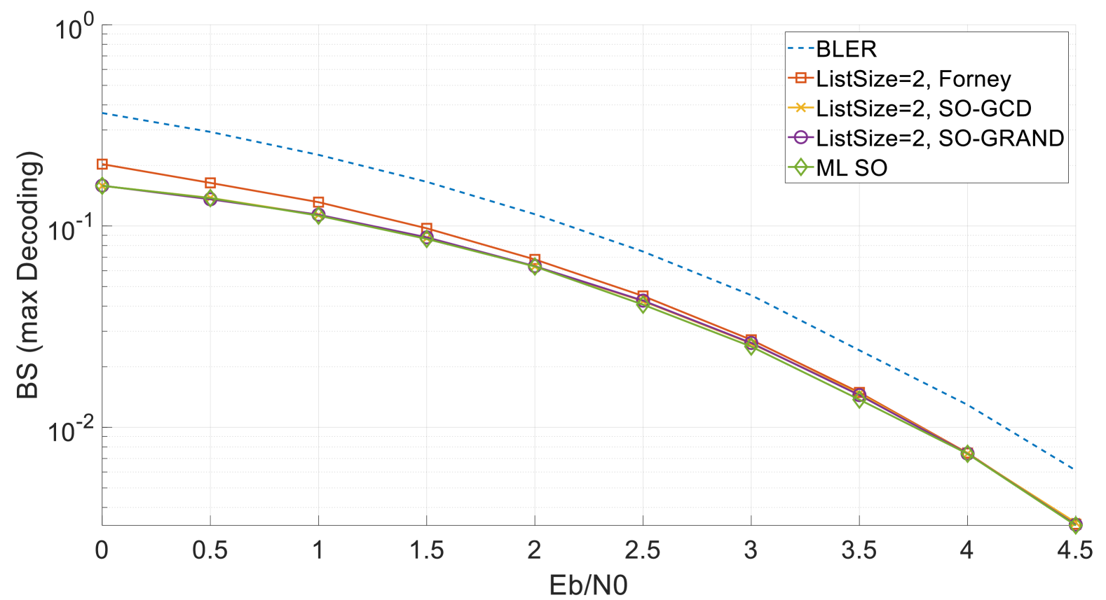
Figure 1: Example of BS vs Eb/N0 using eBCH(16, 11) code.

Fig. 1 presents a comparison of Forney, SO-GCD, SO-GRAND and ML SO when $L=2$. The dashed line indicates the naïve SO of ORBGRAND (ORB), its BLER. The line with diamonds represents ML decoder SO. The line with squares represents Forney’s approximation, eq. (4) where different decoders with the same decoded lists provide the same value. The line with crosses represents SO-GCD, while the line with circles represents SO-GRAND eq. (5). As can be seen, Forney’s approximation has higher BS in lower SNR compared to other SO while SO-GCD and SO-GRAND have almost identical BS to the ML SO, which is the most accurate estimate possible without knowing what codeword was transmitted.

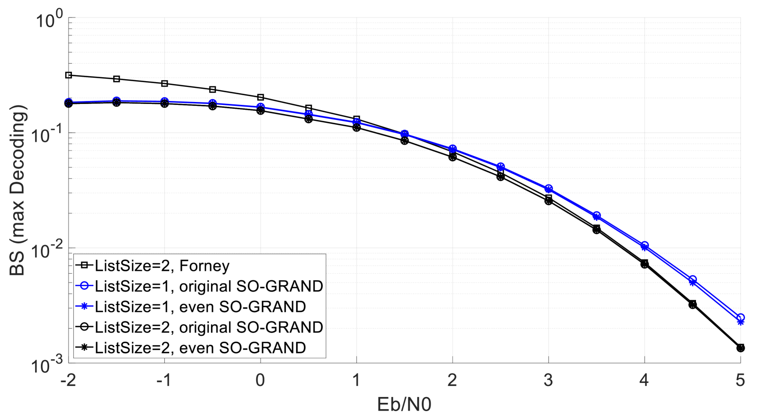
Figure 2: Example of BS using eBCH(16, 11) code.

Fig. 2 investigates the results in Section III and IV. Blue lines represent list size being one while black lines represent list size being two. The line with squares represents Forney’s SO, which requires list size at least two. Lines with circles represent the original SO-GRAND (5) and Lines with stars represent even SO-GRAND (6). Even SO-GRAND provides a better estimate at $L=1$, but the improvement vanishes at $L=2$, which is consistent with the result in Section IV.

VI Conclusions

We demonstrated that binary linear codebook constraints can be leveraged to improve the recently developed blockwise SO from SO-GRAND, SO-GCD (or OSD), and SO-SCL. We introduced a Brier Score scheme by which well-calibrated SO formulas can be assessed. Simulation results using BS suggest that both SO-GRAND and SO-GCD with list size two have almost identical accuracy to a ML SO.

References

- [1] G. Forney, “Exponential error bounds for erasure, list, and decision feedback schemes,” IEEE Trans. Inf. Theory, vol. 14, no. 2, pp. 206–220, 1968.
- [2] R. Pyndiah, “Near-optimum decoding of product codes: block turbo codes,” IEEE Trans. Commun., vol. 46, no. 8, pp. 1003–1010, 1998.
- [3] V. Bioglio, C. Condo, and I. Land, “Construction and decoding of product codes with non-systematic polar codes,” IEEE Wireless Commun. Netw. Conf. (WCNC), pp. 1–6, 2019.
- [4] C. Condo, V. Bioglio, H. Hafermann, and I. Land, “Practical product code construction of polar codes,” IEEE Trans. Signal Process., vol. 68, pp. 2004–2014, 2020.
- [5] M. C. Coşkun, “Precoded polar product codes,” IEEE ISIT, 2024.
- [6] C. Condo, “Iterative soft-input soft-output decoding with ordered reliability bits GRAND,” in IEEE Globecom Wkshp, 2022, pp. 510–515.
- [7] K. Galligan, M. Médard, and K. R. Duffy, “Block turbo decoding with ORBGRAND,” in CISS, 2023.
- [8] A. Solomon, K. R. Duffy, and M. Médard, “Soft maximum likelihood decoding using GRAND,” in IEEE ICC, 2020.
- [9] K. R. Duffy, W. An, and M. Medard, “Ordered reliability bits guessing random additive noise decoding,” IEEE Trans. Signal Proc., vol. 70, pp. 4528 – 4542, 2022.
- [10] W. An, M. Médard, and K. R. Duffy, “Soft decoding without soft demapping with ORBGRAND,” in IEEE ISIT, 2023, pp. 1080–1084.
- [11] K. R. Duffy, M. Grundei, and M. Médard, “Using channel correlation to improve decoding – ORBGRAND-AI,” in IEEE Globecom, 2023.
- [12] A. Riaz, A. Yasar, F. Ercan, W. An, J. Ngo, K. Galligan, M. Médard, K. R. Duffy, and R. T. Yazicigil, “A sub-0.8-pJ/bit universal soft-detection decoder using ORBGRAND,” IEEE J. Solid-State Circuits, 2025.
- [13] K. Galligan, P. Yuan, M. Médard, and K. R. Duffy, “Upgrade error detection to prediction with GRAND,” in IEEE Glob. Commun. Conf., 2023, pp. 1818–1823.
- [14] P. Yuan, M. Medard, K. Galligan, and K. R. Duffy, “Soft-output (SO) GRAND and iterative decoding to outperform LDPC codes,” IEEE Trans. Wireless Commun., to appear.
- [15] X. Ma, “Guessing what, noise or codeword?” IEEE ITW, 2024.
- [16] X. Zheng and X. Ma, “A universal list decoding algorithm with application to decoding of polar codes,” IEEE Trans. Inf. Theory, to appear.
- [17] M. Fossorier and S. Lin, “Soft-decision decoding of linear block codes based on ordered statistics,” IEEE Trans. Inf. Theory, vol. 41, no. 5, pp. 1379–1396, 1995.
- [18] I. Tal and A. Vardy, “List decoding of Polar codes,” IEEE Trans. Inf. Theory, vol. 61, no. 5, pp. 2213–2226, 2015.
- [19] K. R. Duffy, P. Yuan, J. Griffin, and M. Médard, “Soft-output guessing codeword decoding,” IEEE Commun. Lett., to appear.
- [20] P. Yuan, K. R. Duffy, and M. Médard, “Soft-output successive cancellation list decoding,” IEEE Trans. Inf. Theory, 2025.
- [21] M. H. DeGroot and S. E. Fienberg, “The comparison and evaluation of forecasters,” J. Roy. Statistical Soc. Series D, vol. 32, no. 1, pp. 12–22, 1983.
- [22] T. Gneiting and A. E. Raftery, “Strictly proper scoring rules, prediction, and estimation,” J. Am. Stat. Assoc., vol. 102, no. 477, pp. 359–378, 2007.
- [23] D. S. Wilks, Statistical methods in the atmospheric sciences. Academic press, 2011.
- [24] K. R. Duffy, J. Li, and M. Médard, “Capacity-achieving guessing random additive noise decoding,” IEEE Trans. Inf. Theory, vol. 65, no. 7, pp. 4023–4040, 2019.
- [25] M. Rowshan and J. Yuan, “Constrained error pattern generation for GRAND,” in IEEE ISIT, 2022, pp. 1767–1772.
- [26] ——, “Low-complexity GRAND by segmentation,” in IEEE GLOBECOM, 2023, pp. 6145–6151.
- [27] ——, “Segmented GRAND: Combining sub-patterns in near-ML order,” arXiv:2305.14892, 2023.
- [28] J. Griffin, P. Yuan, K. R. Duffy, and M. Medard, “Using a single-parity-check to reduce the guesswork of guessing codeword decoding,” arXiv:2411.09803, 2024.
- [29] E. Arikan, “Channel polarization: A method for constructing capacity-achieving codes for symmetric binary-input memoryless channels,” IEEE Trans. Inf. Theory, vol. 55, no. 7, pp. 3051–3073, 2009.
- [30] P. Koopman and T. Chakravarty, “Cyclic redundancy code (CRC) polynomial selection for embedded networks,” in Int. Conf. on Dep. Sys. and Net., 2004.
- [31] R. Gallager, “Low-density parity-check codes,” IRE Trans. Inf. Theory, vol. 8, no. 1, pp. 21–28, 1962.
- [32] K. R. Duffy, “Ordered reliability bits guessing random additive noise decoding,” in IEEE ICASSP, 2021.
- [33] M. Liu, Y. Wei, Z. Chen, and W. Zhang, “ORBGRAND is almost capacity-achieving,” IEEE Trans. Inf. Theory, vol. 69, no. 5, pp. 2830–2840, 2023.
- [34] H. Gupta, “Partitions–a survey,” J. of Res. Nat. Bur. Standards-B Math. Sci. B, vol. 74, pp. 1–29, 1970.
- [35] A. H. Murphy, “Hedging and skill scores for probability forecasts,” J. Appl. Meteorol. and Climatol., vol. 12, no. 1, pp. 215 – 223, 1973.