Subgradient Method for System Identification with Non-Smooth Objectives

Abstract

This paper investigates a subgradient-based algorithm to solve the system identification problem for linear time-invariant systems with non-smooth objectives. This is essential for robust system identification in safety-critical applications. While existing work provides theoretical exact recovery guarantees using optimization solvers, the design of fast learning algorithms with convergence guarantees for practical use remains unexplored. We analyze the subgradient method in this setting where the optimization problems to be solved change over time as new measurements are taken, and we establish linear convergence results for both the best and Polyak step sizes after a burn-in period. Additionally, we characterize the asymptotic convergence of the best average sub-optimality gap under diminishing and constant step sizes. Finally, we compare the time complexity of standard solvers with the subgradient algorithm and support our findings with experimental results. This is the first work to analyze subgradient algorithms for system identification with non-smooth objectives.

I Introduction

Dynamical systems form the foundation of modern problems, such as reinforcement learning, auto-regressive models, and control systems. These systems evolve based on their current state, with the system dynamics equations determining the next state. Due to the complexity of real-world systems, these dynamics are often unknown or difficult to model precisely. Learning the unknown dynamics of a dynamical system is known as the system identification problem.

The system identification problem has been extensively studied in the literature [1, 2]. The least-squares estimator (LSE) is the most widely studied approach for this problem as it provides a closed-form solution. Early research focused on the asymptotic (infinite-time) convergence properties of LSE [3]. Recently, finite-time (non-asymptotic) analyses gained popularity, leveraging high-dimensional statistical techniques for both linear [4, 5, 6, 7] and nonlinear dynamical systems [8, 9, 10]. See [11] for a survey. Traditionally, both asymptotic and non-asymptotic analyses of LSE focused on systems with independent and identically distributed (sub)-Gaussian disturbances. However, this assumption is often unrealistic for safety-critical systems such as autonomous vehicles, unmanned aerial vehicles, and power grids. In these settings, disturbances may be designed by an adversarial agent, leading to dependencies across time and arbitrary variations.

Since LSE is susceptible to outliers and temporal dependencies, recent research focused on robust non-smooth estimators for safety-critical systems, particularly lasso-type estimators. [12] and [13] analyzed the properties of these estimators through the lens of the Null Space Property, a key concept in lasso analysis. Later works introduced a disturbance structure where disturbance vectors are zero with probability $1-p$ and nonzero with probability $p$. For any $p$ between $0$ and $1$, [14] and [15] proved that lasso-type estimators with non-smooth objectives can exactly recover system dynamics for linear and parameterized nonlinear systems, respectively, with probability approaching one. Additionally, [16] showed that asymmetric disturbances with nonzero probability $p$ could be transformed into zero-mean disturbances with probability $2p$, enabling exact recovery for any disturbance structure where $p<1/2$. These non-asymptotic analyses leverage techniques from modern high-dimensional probability and statistics [17, 18]. Despite their strong learning properties, these approaches rely on convex optimization solvers, which become computationally prohibitive as the system state dimension and time horizon grow. Safety-critical systems require rapid estimation to ensure real-time control without delays. Thus, it is imperative to design fast algorithms that efficiently solve lasso-type non-smooth estimators within a reasonable time frame.

Due to the non-smoothness of the objective, gradient- and Hessian-based first-order and second-order algorithms are not viable options in this context. Instead, we employ the subgradient method, a well-established technique in the literature, as the lasso-type estimator is a convex optimization problem. Unlike gradient-based methods, subgradient methods do not guarantee descent at each iteration. However, existing results show that the best sub-optimality gap asymptotically converges to zero over time with both constant and diminishing step sizes. For a comprehensive overview of subgradient methods for non-smooth objectives, see [19, 20, 21, 22, 23]. Closed-form solutions and gradient-based methods are widely used in system identification problems, as the literature has primarily focused on LSE or other smooth estimators for linear systems [24]. Nonlinear system identification is inherently more complex than its linear counterpart [25], yet existing estimation techniques still rely on smooth penalty functions. In contrast, subgradient methods have not been explored in the system identification context. Thus, this paper is the first to analyze the subgradient algorithm for the system identification problem. It is important to note that we do not apply the subgradient method to a single optimization problem and instead apply it to a sequence of time-varying problems due to the fact that as new measurements are taken, the optimization problem to be solved changes as well.

Notations: For a matrix $Z$, $\|Z\|_{F}$ denotes its Frobenius norm. For two matrices $Z_{1}$ and $Z_{2}$, we use $\langle Z_{1},Z_{2}\rangle$ and $Z_{1}\otimes Z_{2}$ to denote the inner product and Kronecker product, respectively. For a matrix $Z$, $\operatorname{vec}(Z)$ is the usual vectorization operation by stacking the columns of the matrix $Z$ into a vector. For a vector $z$, $\|z\|_{2}$ denotes its $\ell_{2}$-norm. $\angle z_{1}z_{2}$ denotes the angle between two vectors and $\angle\operatorname{vec}(Z_{1})\operatorname{vec}(Z_{2})$ is the angle between two matrices $Z_{1}$ and $Z_{2}$. Given two functions $f$ and $g$, the notation $f(x)=\Theta(g(x))$ means that there exist universal positive constants $c_{1}$ and $c_{2}$ such that $c_{1}g(x)\leq f(x)\leq c_{2}g(x)$. Similarly, $f(x)\leq\mathcal{O}(g(x))$ implies that there exists a universal positive constant $c_{3}$ such that $f(x)\leq c_{3}g(x)$. $I_{n}$ stands for the $n\times n$ identity matrix and $0_{n}$ is the vector of zeros with dimension $n$.

II Non-smooth Estimator and Disturbance Model

We consider a linear time-invariant dynamical system of order $n$ with the system update equation

$$x_{t+1}=\bar{A}x_{t}+\bar{d}_{t},\quad t=0,1,\dots,T-1,$$

where $\bar{A}\in\mathbb{R}^{n\times n}$ is the unknown system matrix and $\bar{d}_{t}\in\mathbb{R}^{n}$ are unknown system disturbances. Our goal is to estimate $\bar{A}$ using the state samples $\{x_{t}\}_{t=0}^{T}$ obtained from a single system initialization. Note we only study the autonomous case due to space restrictions and the generalization to the case with inputs is straightforward. Traditionally, the following LSE has been widely studied in the literature:

$$\min_{A\in\mathbb{R}^{n\times n}}\;\,\sum_{i=0}^{T-1}\lVert x_{t+1}-Ax_{t}\rVert_{2}^{2}.$$ (LSE)

However, the LSE is vulnerable to outliers and adversarial disturbances. In safety-critical system identification, a new popular alternative is the following non-smooth estimator:

$$\min_{A\in\mathbb{R}^{n\times n}}\;\,\sum_{i=0}^{T-1}\lVert x_{t+1}-Ax_{t}\rVert_{2}.$$ (NSE)

The primary objective of this non-smooth estimator is to achieve exact recovery in finite time, which is an essential feature for safety-critical applications such as power-grid monitoring, unmanned aerial vehicles, and autonomous vehicles. In these scenarios, the system should be learned from a single trajectory (since multiple initialization is often infeasible) and, moreover, it can be exposed to adversarial agents. Even under i.i.d. disturbance vectors, if $\bar{d}_{t}$ is non-zero at every time step $t$, the exact recovery of the $\bar{A}$ is not attainable in finite time. Motivated by [15], we, therefore, introduce a disturbance model in which the disturbance vector $\bar{d}_{t}$ is zero at certain time instances.

Definition 1 (Probabilistic sparsity model [15]).

For each time instance $t$, the disturbance vector $\bar{d}_{t}$ is zero with probability $1-p$, where $p\in(0,1)$. Furthermore, the time instances at which the disturbances are nonzero are independent of each other (while the nonzero disturbance values could be correlated).

[15] showed that the estimator (LSE) fails to achieve exact recovery in finite time even when $p<1$ and in the simplest case when the disturbance vectors are i.i.d. Gaussian. Consequently, it becomes essential to employ non-smooth estimators to enable exact recovery within a finite time horizon. Furthermore, without specific assumptions on the system dynamics and disturbance vectors, exact recovery is unattainable in finite time. See Theorem 3 in [15]. First, we impose a sufficient condition for the system stability of the LTI system in Assumption 1 to guarantee learning under possibly large correlated disturbances.

Assumption 1.

The ground-truth $\bar{A}$ satisfies $\rho:=\left\|\bar{A}\right\|_{2}<1$.

If the disturbance vectors take arbitrary values and are chosen from a low-dimensional subspace, it is shown in [15] that learning the full system dynamics becomes infeasible. To address this, we define the filtration $\mathcal{F}_{t}:=\sigma\{x_{0},x_{1},\dots,x_{t}\}$, and we add the semi-oblivious and sub-Gaussian disturbances assumption below based on [15].

Assumption 2 (Semi-Oblivious and sub-Gaussian disturbances).

Conditional on the filtration $\mathcal{F}_{t}$ and the event that $\bar{d}_{t}\neq 0_{n}$, the attack vector $\bar{d}_{t}$ is defined by the product $\ell_{t}\hat{d}_{t}$, where

1. $\hat{d}_{t}\in\mathbb{R}^{n}$ and $\ell_{t}\in\mathbb{R}$ are independent conditional on $\mathcal{F}_{t}$ and $\bar{d}_{t}\neq 0_{n}$;

2. $\hat{d}_{t}$ obeys the uniform distribution on the unit sphere whenever $\bar{d}_{t}\neq 0_{n}$;

3. $\ell_{t}$ is zero-mean and sub-Gaussian with parameter $\sigma$.

Assumption 2 implies that the disturbance vectors $\bar{d}_{t}$ are sub-Gaussian and temporally correlated (since $\ell_{t}$ may depend on previous disturbances). This correlation better reflects real-world semi-oblivious attacks, where an adversarial agent can inject disturbances that depend on prior injections. Moreover, Assumption 2 ensures exploration of the entire state space, as the direction vector $\hat{d}_{t}$ is uniformly distributed on the unit sphere.

In recent years, non-smooth estimators for system identification gained traction [26, 27, 14, 15, 16]. These studies analyzed non-smooth estimators in a non-asymptotic framework under various disturbance models. Specifically, under Assumptions 1 and 2, [14] and [15] derived sample complexity bounds for exact recovery in finite time with high probability. However, they do not propose numerical algorithms and rely on existing convex optimization solvers, which suffer from two drawbacks. The first issue is that in practice (NSE) should be repeatedly solved for $T=1,2,...$ as new measurements are taken until a satisfactory model is obtained. This means that the methods in [15] and [16] require solving a convex optimization problem at each time step. In addition, the problem (NSE) at time $T$ is translated into a second-order conic program with $T+n^{2}$ scalar variables and $T$ conic inequalities. Hence, the solver performance degrades significantly as the order of the system and the time horizon grow. Since safety-critical applications demand fast and efficient identification, convex optimization solvers are inefficient for real-time computation. To address these limitations, we investigate the subgradient method for learning system parameters.

III Subgradient Method

Let $f_{T}(A)$ denote the objective function of (NSE) and $\partial f_{T}(A)$ denote its subdifferential at a point $A$ and time period $T$. We denote a subgradient in the subdifferential as $G_{A,T}\in\partial f_{T}(A)$. We first define the subdifferential of the $\ell_{2}$ norm.

Definition 2 (Subdifferential of $\ell_{2}$ Norm).

Let $\partial\|x\|_{2}$ denote the subdifferential of the $\ell_{2}$ norm, i.e.,

$$\partial\|x\|_{2}=\begin{cases}\frac{x}{\|x\|_{2}},&\text{if }x\not=0,\\ \{e:\|e\|_{2}\leq 1\},&\text{otherwise }.\end{cases}$$

The subdifferential is a unique point when $x$ is nonzero, but it consists of all points within the unit ball when $x=0$. Using the previous definition, we obtain the subdifferential of the objective function, $\partial f_{T}(A)$.

Lemma 1.

The subdifferential of $f_{T}(\cdot)$ at a point $A$ is

$$\partial f_{T}(A)=\left\{-\sum_{t=0}^{T-1}\partial\|x_{t+1}-Ax_{t}\|_{2}\otimes x_{t}\right\},$$

and the subdifferential of the $f_{T}(\cdot)$ at the point $\bar{A}$ is

$$\partial f_{T}(\bar{A})=\left\{-\sum_{t\in\mathcal{K}}\hat{d}_{t}\otimes x_{t}-\sum_{t\not\in\mathcal{K}}e_{t}\otimes x_{t}:\|e_{t}\|_{2}\leq 1,\forall t\not\in\mathcal{K}\right\},$$

where $\mathcal{K}:=\{t~|~\bar{d}_{t}\neq 0\}$ is the set of time indices of nonzero disturbances and $\hat{d}_{t}:=\bar{d}_{t}/\|\bar{d}_{t}\|_{2},\forall t\in\mathcal{K}$, are the normalized disturbance directions.

The proof of Lemma 1 is straightforward and follows from a property of the Minkowski sum over convex sets. Furthermore, due to the convexity of $f_{T}(A)$, the next lemma provides a useful bound on the difference between the objective function values at two distinct points.

Lemma 2 ([28]).

Given two arbitrary points $A,B\in\mathbb{R}^{n\times n}$ and any subgradient $G_{A,T}\in\partial f_{T}(A)$, it holds that

$$f_{T}(B)\geq f_{T}(A)+\langle G_{A,T},B-A\rangle.$$

To find the matrix $\bar{A}$, we propose Algorithm 1 that relies on the subgradient method. In Step (i), the subdifferential of the objective function at the current estimate is calculated. Since this subdifferential possibly contains multiple values, we choose a subgradient from the subdifferential in Step (ii). After that, a step size is selected in Step (iii). In Step (iv), a subgradient update is performed. Lastly, we update the objective function with the new data point in Step (v). The main feature of this algorithm is that we do not apply the subgradient algorithm to solve the current optimization problem (NSE) and instead we take one iteration to update our estimate of the matrix value at time $t$. Then, after a new measurement is taken, the optimization problem at time $t+1$ changes since an additional term is added to its objective function. Thus, as we update our estimates, the optimization problems also change over time. We analyze the convergence of Algorithm 1 under different step size selection rules and show that although the objective function changes at each iteration, our algorithm convergences to the $\bar{A}$.

Algorithm 1 Subgradient Method for (NSE)

 Initialize $\hat{A}^{(0)}$ randomly

 for $t=0,\dots,T-1$ do

  (i) Find $\partial f_{t}(\hat{A}^{(t)})=-\sum_{\ell=0}^{t}\partial\lVert(\bar{A}-\hat{A}^{(t)})x_{\ell}+\bar{d}_{\ell}\rVert_{2}\otimes x_{\ell}$

  (ii) Choose $G_{\hat{A}^{(t)},t}$ from $\partial f_{t}(\hat{A}^{(t)})$

  (iii) Choose $\beta^{(t)}$ using an appropriate step size rule

  (iv) Update $\hat{A}^{(t+1)}=\hat{A}^{(t)}-\beta^{(t)}G_{\hat{A}^{(t)},t}$

  (v) Update $f_{t+1}(A)=f_{t}(A)+\|x_{t+1}-Ax_{t}\|_{2}$

 end for

 Return $\hat{A}^{(T)}$

III-A Subgradient Method with Best Step Size

We analyze the subgradient method using the best step size, which is defined as the step size that maximizes improvement at each iteration. However, computing this step size requires knowledge of the ground-truth matrix $\bar{A}$, making it impractical in real-world applications. Nonetheless, studying this case offers valuable insights into the behavior of subgradient updates. Let the step size in Algorithm 1 be chosen as

$$\beta^{(t)}=\frac{\langle G_{\hat{A}^{(t)},t},\hat{A}^{(t)}-\bar{A}\rangle}{\|G_{\hat{A}^{(t)},t}\|_{F}^{2}},$$

It is shown in Appendix VII-A that this is the best step size possible. According to Theorem 1, the distance to the ground-truth matrix decreases by a factor of $\sqrt{1-\cos^{2}({\hat{\theta}_{t}})}$ at each update with best step size. As long as this angle is not $\pm 90^{\circ}$ or $\pm 270^{\circ}$, Algorithm 1 makes progress toward $\bar{A}$.

Theorem 1.

Under the best step size for Algorithm 1, it holds that

$$\|\hat{A}^{(t+1)}-\bar{A}\|_{F}\leq\sqrt{1-\cos^{2}({\hat{\theta}_{t}})}\|\hat{A}^{(t)}-\bar{A}\|_{F},$$

where $\hat{\theta}_{T}$ denotes the angle between $\hat{A}^{(t)}-\bar{A}$ and $G_{\hat{A}^{(t)},t}$.

If $\hat{\theta}_{t}$ is obtuse, the step size will be negative, which must be avoided. To this end, we establish a positive lower bound on $\cos(\hat{\theta}_{t})$ in Theorem 2 and show that this angle remains acute. To guarantee that, we define the burn-in period as the number of samples required for a theoretical exact recovery. After the burn-in period, $\bar{A}$ is the unique optimal solution of $\min f_{T}(A)$ with high probability.

Definition 3.

Consider an arbitrary $\delta\in(0,1)$. Let $T^{(burn)}(n,p,\rho,\sigma,\delta)$ be defined as

$$T^{(burn)} :=\Theta\Bigg{(}\max\left\{\frac{\sigma^{10}}{(1-\rho)^{3}(1-p)^{2}},\frac{\sigma^{4}}{p(1-p)}\right\}$$

$$\times\left[n^{2}\log\left(\frac{1}{(1-\rho)\sigma p(1-p)}\right)+\log\left(\frac{1}{\delta}\right)\right]\Bigg{)}.$$

For every $t\geq T^{(burn)}(n,p,\rho,\sigma,\delta)$, $\bar{A}$ is the unique optimal solution to (NSE) with probability at least $1-\delta$.

For convenience, we omit the argument $(n,p,\rho,\sigma,\delta)$ and denote the burn-in period as $T^{(burn)}$. We analyze the algorithm’s behavior after the burn-in period because it happens that the iterates of Algorithm 1 are chaotic when $t$ is not large enough or equivalently when $\bar{A}$ is not the unique solution of (NSE). The following theorem establishes that if the number of samples exceeds $T^{(burn)}$, the cosine of the angle can be lower-bounded by a positive term.

Theorem 2.

Define $\hat{\theta}_{T}$ to be the angle between $\hat{A}^{(T)}-\bar{A}$ and $G_{\hat{A}^{(T)},T}$, and let $\widetilde{\|x_{T}\|_{2}}=\sum_{i=0}^{T-1}\|x_{t}\|_{2}/T$ be the average norm of the states until time $T$. Suppose that Assumptions 1 and 2 hold. Then, as long as the sample complexity $T\geq T^{(burn)}(n,p,\rho,\sigma,\delta)$ and $\hat{A}^{(T)}\neq\bar{A}$, with probability at least $1-\delta$, the term $\cos({\hat{\theta}_{T}})$ can be lower-bounded as

$$\cos({\hat{\theta}_{T}})\geq\Theta\left(\min\left\{1,\frac{p(1-p)}{\sigma^{4}\widetilde{\|x_{T}\|_{2}}}\right\}\right)>0.$$

Theorem 2 provides a probabilistic lower bound on the cosine of the angle of interest when the sample complexity $T$ is sufficiently large. The algorithm iterates move toward the ground truth $\bar{A}$ when the $\bar{A}$ is the global solution of (NSE). In this lower bound, the average norm of the system states over time, $\widetilde{\|x_{T}\|_{2}}$, appears as a random variable. This term is known to have an upper bound on the order of $p^{1/2}/\sigma^{9}(1-\rho)$ with high probability.

Lemma 3 (Equation (63) in [15]).

Under the assumptions of Theorem 2, when $T\geq T^{(burn)}(n,p,\rho,\sigma,\delta)$, the inequality

$$\widetilde{\|x_{T}\|_{2}}\leq\Theta\left(\frac{p^{1/2}}{\sigma^{9}(1-\rho)}\right)$$

holds with probability at least $1-\delta$

In order to establish the result in Lemma 3, we select $\theta:=\Theta(p(1-p)T/\sigma^{4})$ and $\epsilon:=\Theta(\sqrt{p(1-p)^{2}(1-\rho)^{2}\sigma^{10}})$ in Equation (63) of [15]. Combining this result with Theorem 2 leads to the main result of this subsection.

Corollary 1.

Let $D=\|\hat{A}^{(T^{(burn)}(n,p,\rho,\sigma,\delta/2))}-\bar{A}\|_{F}$ denote the distance of the solution of the last iterate to the ground-truth $\bar{A}$ at the end of the burn-in time. Define $\gamma(p,\rho,\sigma)$ to be

$$\gamma(p,\rho,\sigma):=\sqrt{1-\min\{1,\Theta(p(1-p)^{2}\sigma^{10}(1-\rho)^{2})\}}.$$

Then, given an arbitrary $\epsilon>0$, Algorithm 1 under the best step size achieves $\|\hat{A}^{(T)}-\bar{A}\|_{F}\leq\epsilon$ with probability $1-\delta$, when the number of iterations $T$ is sufficiently large such that $T>T^{(\epsilon)}:=T^{(burn)}(n,p,\rho,\sigma,\delta/2)+T^{(conv)}(p,\rho,\sigma,D,\epsilon)$, where

$$T^{(conv)}(p,\rho,\sigma,D,\epsilon):=\log\left(\frac{D}{\epsilon}\right)\log\left(\frac{1}{\gamma(p,\rho,\sigma)}\right).$$

Algorithm 1 achieves linear convergence with high probability after the burn-in period due to the $\log(D/\epsilon)$ term. Corollary 1 implies that to achieve an $\epsilon$-level estimation error, the total number of required samples should be the sum of those needed for the burn-in phase and the linear convergence phase. With high probability, the burn-in period scales as $\max\{(1-p)^{-2},p^{-1}(1-p)^{-1}\}$ with respect to $p$ and as $n^{2}$ with respect to the system dimension. After the burn-in phase, the algorithm converges to the ground truth at a linear rate because $\cos(\hat{\theta}_{T})$ is lower-bounded by a positive factor given by $\min\{1,p^{1/2}(1-p)\sigma^{5}(1-\rho)\}$. Consequently, the linear convergence is upper-bounded by $\gamma(p,\rho,\sigma)$, and the sample complexity scales logarithmically with the problem parameters. Therefore, the sample complexity of the burn-in period dominates the sample complexity of the linear convergence phase. Next, we now generalize the results to more practical step size rules.

III-B Subgradient Method with Polyak Step Size

We analyze the Polyak step size. Unlike the best step size selection, the Polyak step size does not require knowledge of $\bar{A}$. However, it requires information about the optimal objective value at $\bar{A}$ at time $T$, that is $f_{T}(\bar{A})$. Under this step size rule, we can establish a result similar to Corollary 1.

Theorem 3.

Consider Algorithm 1 under the Polyak step size defined as

$$\beta^{(T)}=\frac{(f_{T}(\hat{A}^{(T)})-f_{T}(\bar{A}))}{\|G_{\hat{A}^{(T)},T}\|_{F}^{2}}.$$

Suppose that Assumptions 1 and 2 hold. When the number of samples $T$ is greater than $T^{(\epsilon)}$, Algorithm 1 achieves $\|\hat{A}^{(T)}-\bar{A}\|_{F}\leq\epsilon$, where $T^{(\epsilon)}$ defined in Corollary 1.

Although the Polyak step size relies on less information about the ground-truth system dynamics than the best step size (i.e., it needs to know an optimal scalar rather than an optimal matrix), it requires the same number of iterations as the best step size selection. These step sizes are implementable in practice (subject to some approximations) if some prior knowledge about the system dynamics is available.

III-C Subgradient Method with Constant and Diminishing Step Sizes

The step sizes discussed in previous sections require information about the ground-truth matrix $\bar{A}$ and the optimal objective value $f_{T}(\bar{A})$. While theoretically useful, these step sizes are impractical in real-world applications. Therefore, we explore the subgradient method with constant and diminishing step sizes. Unlike the best and Polyak step sizes, constant and diminishing step sizes do not guarantee descent at every iteration. Instead, they lead to convergence within a neighborhood of the true solution rather than exact recovery. Consequently, results concerning the solution gap, $\hat{A}^{(T)}-\bar{A}$, are less relevant in this setting. Nevertheless, we establish the asymptotic convergence of the best average sub-optimality gap over time, defined as:

$$\min_{t\in[T^{(burn)}(n,p,\rho,\sigma,\delta),T]}\left\{\frac{1}{t}(f_{t}(\hat{A}^{(t)})-f_{t}(\bar{A}))\right\}.$$

The best average sub-optimality gap represents the algorithm’s performance over its entire horizon, from the burn-in period to the final iteration. We scale the sub-optimality gap by $1/t$ to ensure comparability across time steps, as the objective function $f_{t}(A)$ in (NSE) evolves with $t$ and consists of a sum of $t$ terms. An $\epsilon$-level estimation error at time $t$ , i.e. $\|\hat{A}^{(t)}-\bar{A}\|_{F}\leq\epsilon$, corresponds to a sub-optimality gap of $t\epsilon$. Furthermore, we focus on the best average sub-optimality gap rather than the gap at the final iteration, as iterates fluctuate around the neighborhood of $\bar{A}$ due to the nature of these step sizes. These step sizes may potentially remain large, preventing exact convergence, or diminish too quickly or too slowly to achieve a precise limit. Additionally, we analyze the best average sub-optimality gap only after the burn-in period since $\bar{A}$ may not be the global minimizer during this phase, leading to potential negative sub-optimality terms.

Next, we demonstrate that under a constant step size, the best average sub-optimality gap of the subgradient algorithm asymptotically converges at a rate of $T^{-1/2}$. When $T$ is significantly larger than $T^{(burn)}$, the upper bound for the best average sub-optimality gap can be simplified as $\Theta(Dp^{1/2}/\sigma^{9}(1-\rho)T^{1/2})$. Hence, it asymptotically converges to zero with the rate $T^{-1/2}$.

Theorem 4.

When the step size $\beta^{(t)}$ is set to the constant,

$$\beta^{(t)}=\beta=\Theta\left(\frac{D\sigma^{9}(1-\rho)}{p^{1/2}(\sum_{t=T^{(burn)}}^{T}t^{2})^{1/2}}\right),$$

the best average sub-optimality gap for Algorithm 1 iterates can be bounded with probability at least $1-\delta$ as

$$\min_{t\in[T^{(burn)},T]} \left\{\frac{1}{t}(f_{t}(\hat{A}^{(t)})-f_{t}(\bar{A}))\right\}$$

$$\leq\Theta\left(\frac{Dp^{1/2}}{\sigma^{9}(1-\rho)}\times\frac{(\sum_{t=T^{(burn)}}^{T}t^{2})^{1/2}}{\sum_{t=T^{(burn)}}^{T}t}\right).$$

We establish a similar result for the diminishing step size.

Theorem 5.

Suppose that the step size $\beta^{(t)}$ takes the diminishing form $\beta^{(t)}=\beta/t$, where $\beta$ is defined as

$$\beta:=\Theta\left(\frac{D\sigma^{9}(1-\rho)}{p^{1/2}(T-T^{(burn)})^{1/2}}\right).$$

Then, with probability at least $1-\delta$, the best average sub-optimality gap for Algorithm 1 iterates can be bounded as

$$\min_{t\in[T^{(burn)},T]} \left\{\frac{1}{t}(f_{t}(\hat{A}^{(t)})-f_{t}(\bar{A}))\right\}$$

$$\leq\Theta\left(\frac{Dp^{1/2}}{\sigma^{9}(1-\rho)}\times\frac{1}{(T-T^{(burn)})^{1/2}}\right).$$

The proof of Theorem 5 is omitted as it follows the same reasoning as Theorem 4. The diminishing step size is chosen to satisfy $\sum\beta^{(t)}\xrightarrow{}\infty$ and $\sum(\beta^{(t)})^{2}<\infty$, ensuring sufficient exploration and stable convergence without excessive oscillations. Theorem 5 establishes that, under a diminishing step size, the best average sub-optimality gap asymptotically converges at a rate of $T^{-1/2}$.

IV Time Complexity Analysis

We compare the time complexities of the subgradient method and the exact solution of (NSE) using CVX. For the subgradient algorithm, each time period involves computing the subgradient, which has a per-iteration cost of $\mathcal{O}(Tn^{2})$. Running the algorithm for $T$ iterations results in an overall complexity of $\mathcal{O}(T^{2}n^{2})$. On the other hand, solving (NSE) using CVX reduces the problem to a second-order conic program (SOCP) with $T+n^{2}$ variables with $T$ second-order cone constraints (minimization of the sum of norms can be written as a SOCP [29]). Defining $[T]=\{0,1,\dots,T-1\}$, this problem is formulated as

$$\min_{\begin{subarray}{c}vec(A)\in\mathbb{R}^{n^{2}}\\ f_{t}\in\mathbb{R},\;t\in[T]\end{subarray}} \quad\sum_{t=0}^{T}f_{t}$$ (SOCP)

s.t. $$f_{t}\geq\|x_{t+1}-(x_{t}\otimes I_{n})vec(A)\|_{2},\;t\in[T].$$

The CVX solver employs primal-dual interior point methods to solve (SOCP). The number of iterations required to reach an $\epsilon$-accurate solution is $\mathcal{O}(T^{1/2}\log(1/\epsilon))$ [30]. Since solving conic constraints has a worst-case complexity of $\mathcal{O}(n^{6})$, the per time period complexity is $\mathcal{O}(T^{1/2}n^{6})$, leading to an overall complexity of $\mathcal{O}(T^{3/2}n^{6})$. We know that $T$ and $T^{(burn)}$ scale as $\Theta(n^{2})$. Consequently, the per-time period complexity of the subgradient method and the exact SOCP solution are $\mathcal{O}(n^{4})$ and $\mathcal{O}(n^{7})$, respectively. This highlights that solving (SOCP) exactly requires significantly more computational power than the subgradient approach. Next, we present numerical experiments to validate the convergence results.

V Numerical Experiments

We generate a system with ground-truth matrix $\bar{A}$ whose singular values are uniform in $(0,1)$. Given the probability $p$, disturbance vectors are set to zero with probability $1-p$. With probability $p$, the disturbance $\bar{d}_{t}$ is defined as $\bar{d}_{t}:=\ell_{t}\hat{d}_{t}$. Then, we sample $\ell_{t}\sim\mathcal{N}(0,\sigma_{t}^{2})$, where $\sigma_{t}^{2}:=\min\{\|x_{t}\|_{2}^{2},1/n\}$, and we sample $\hat{d}_{t}\sim\mathrm{uniform}(\mathbb{S}^{n-1})$. This disturbance vector conforms to Assumption 2, and the values of the disturbance vectors are correlated over time. We generate $10$ independent trajectories of the subgradient algorithm using $10$ different systems. Then, we report the average solution gap and the average loss gap of Algorithm 1 at each period. The solution gap and the loss gap for Algorithm 1 at time $T$ are $\|\hat{A}^{(T)}-\bar{A}\|_{F}$ and $f_{T}(\hat{A}^{(T)})-f_{T}(\bar{A})$, respectively.

Algorithm 1 is experimented with different step size rules. The system has order $n=5$, and $p=0.7$. In addition to the best, Polyak, diminishing, and constant step sizes, we also introduce the backtracking step size. We initialize the step size at a constant value, and it is shrunk by constant factor $\gamma\in(0,1)$ until we achieve a sufficiently large descent. See Armijo step size in [31]. Figure 1 depicts the performance of Algorithm 1 under these different step sizes. Best and Polyak step sizes achieve fast and linear convergence as proven theoretically. Moreover, the backtracking step size performs similarly to the best and Polyak step sizes without using the knowledge of the ground truth $\bar{A}$ or the optimal objective value $f_{T}(\bar{A})$. Thus, the theoretical analysis of the backtracking step size is an interesting future direction. Furthermore, despite the slower rates, the diminishing and constant step sizes converged to the neighborhood of the solution.

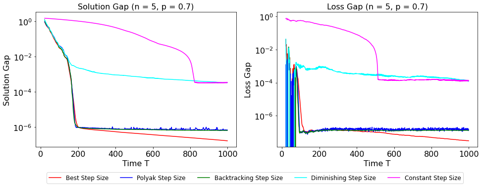
Figure 1: Solution Gap and Loss Gap of Algorithm 1 with Different Step Sizes for $n=5$, and $p=0.7$

We test the performance of Algorithm 1 with different system dimensions $n$ and different probabilistic sparsity model parameters $p$. We choose backtracking and best step sizes to test the impact of different dimensions of the system states, $n\in\{5,10,15\}$ on the solution gap and loss gap when $p$ is set to $0.7$. Figure 2 shows that as $n$ grows, the number of samples needed for convergence grows as $n^{2}$. This aligns with the theoretical results from earlier sections. Moreover, the backtracking step size performs similarly to the best step size. Likewise, Figure 3 depicts the performance of the subgradient algorithm for the different probabilities of nonzero disturbance $p\in\{0.5,0.7,0.8\}$ with $n=5$ using best and backtracking step sizes. As $p$ increases, the convergence for the estimator needs more samples, as supported by the theoretical results.

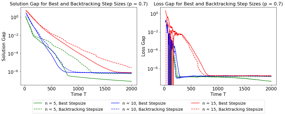
Figure 2: Solution Gap and Loss Gap of Algorithm 1 with $p=0.7$, Best and Backtracking Step Sizes, and $n\in\{5,10,15\}$

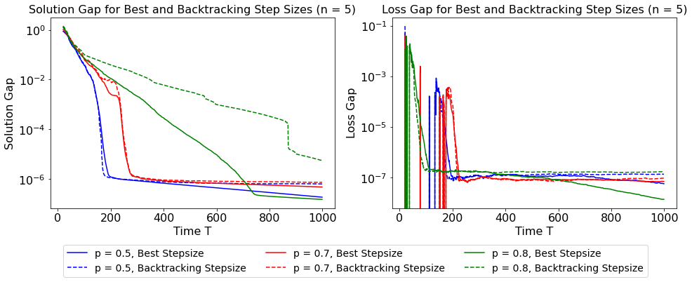
Figure 3: Solution Gap and Loss Gap of Algorithm 1 with $n=5$, Best and Backtracking Step Sizes, and $p\in\{0.5,0.7,0.8\}$

We perform experimentation on the subgradient selection in Step (ii) of Algorithm 1. Whenever the $\ell_{2}$ norm is less than $10^{-5}$, we consider its subdifferential as the unit ball. For random subgradient selection, we select the subgradient randomly on the unit sphere. For the zero subgradients, we set the subgradient to zero. Lastly, we chose the minimum norm subgradient among all the available ones in the subdifferential. We test these selection criteria for a system with order $n=10$ and $p=0.7$ using the best step size. Figure 4 demonstrates that there is not a significant difference in terms of solution gap.

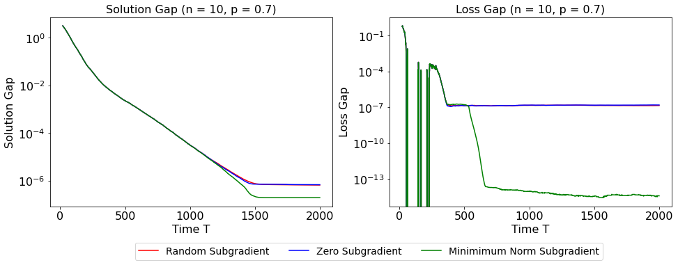
Figure 4: Solution Gap and Loss Gap of Algorithm 1 with Different Subgradient Selection Methods for $n=10$ and $p=0.7$

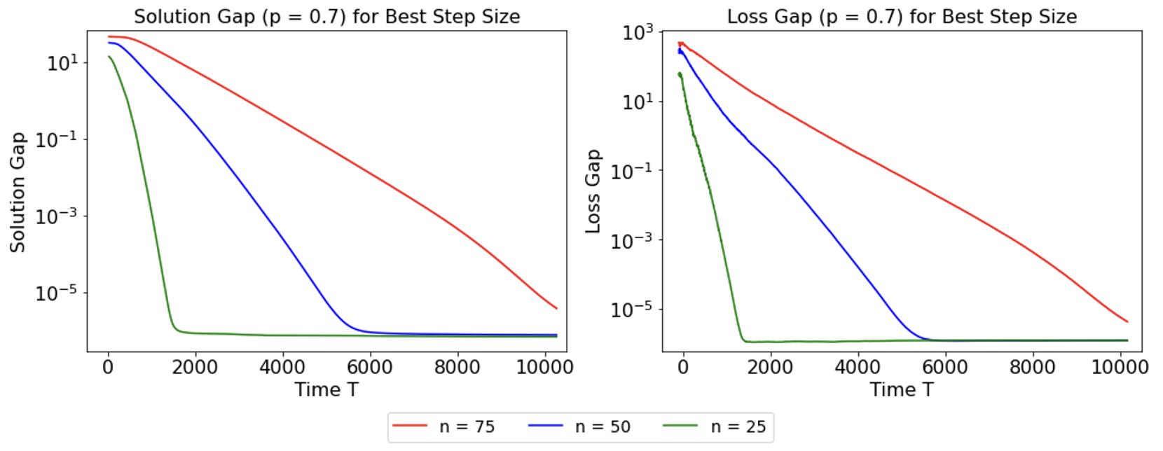
Figure 5: Solution Gap and Loss Gap of Algorithm 1 with $p=0.7$, Best Step Size, and $n\in\{50,75,100\}$

Last but not least, we provide simulation results using the best step size for large systems of order $n\in\{25,50,75\}$. We run these experiments for $T=10000$. This is not possible with the CVX solver due to the high computational complexity of (SOCP). Nevertheless, the subgradient algorithm provides an accurate estimation for large systems within a reasonable time frame, as seen in Figure 5.

VI Conclusion

We proposed and analyzed a subgradient algorithm for non-smooth system identification of linear-time invariant systems with disturbances following a probabilistic sparsity model. While the non-asymptotic theory for this setting is well-established in the literature, existing methods rely on solvers that use primal-dual interior-point methods for second-order conic programs, leading to high computational costs. To address this, we proposed a subgradient method that enables fast exact recovery. We demonstrated that the subgradient method with the best and Polyak step sizes converges linearly to the ground-truth system dynamics after a burn-in period. Additionally, we showed that constant and diminishing step sizes lead to convergence within a neighborhood of the true solution, with the best average sub-optimality gap asymptotically approaching zero. These theoretical results are supported by numerical simulations.

Our experiments also highlight the practical effectiveness of the backtracking step size, suggesting it as a promising alternative. However, its theoretical properties remain an open question. Furthermore, our current implementation computes the full subgradient at each iteration. To improve time complexity, a partial subgradient approach, similar to stochastic gradient descent, could be explored.

VII Appendix

VII-A Proof of Theorem 1

Proof.

Using the subgradient update iteration at time $T$, $\hat{A}^{(T+1)}=\hat{A}^{(T)}-\beta^{(T)}G_{\hat{A}^{(T)},T}$, we have

$$\|\hat{A}^{(T+1)}-\bar{A}\|_{F}^{2} =\|(\hat{A}^{(T)}-\bar{A})-\beta^{(T)}G_{\hat{A}^{(T)},T}\|_{F}^{2}$$

$$=\|\hat{A}^{(T)}-\bar{A}\|_{F}^{2}+(\beta^{(T)})^{2}\|G_{\hat{A}^{(T)},T}\|_{F}^{2}$$

$$-2\beta^{(T)}\langle G_{\hat{A}^{(T)},T},\hat{A}^{(T)}-\bar{A}\rangle.$$ (1)

Substituting the step size stated in the theorem yields

$$\|\hat{A}^{(T+1)}-\bar{A}\|_{F}^{2} =\|\hat{A}^{(T)}-\bar{A}\|_{F}^{2}-\frac{(\langle G_{\hat{A}^{(T)},T},\hat{A}^{(T)}-\bar{A}\rangle)^{2}}{\|G_{\hat{A}^{(T)},T}\|_{F}^{2}}$$

$$\leq\sqrt{1-\cos^{2}({\hat{\theta}_{T}})}\|\hat{A}^{(T)}-\bar{A}\|_{F}.$$

The last inequality uses the fact that $\langle G_{\hat{A}^{(T)},T},\hat{A}^{(T)}-\bar{A}\rangle=\|G_{\hat{A}^{(T)},T}\|_{F}\|\hat{A}^{(T)}-\bar{A}\|_{F}\cos({\hat{\theta}_{T}})$.

VII-B Proof of Theorem 2

Proof.

Using Lemma 2, we can show that

$$\cos({\hat{\theta}_{T}})=\frac{\langle\hat{A}^{(T)}-\bar{A},G_{\hat{A}^{(T)},T}\rangle}{\|\hat{A}^{(T)}-\bar{A}\|_{F}\|G_{\hat{A}^{(T)},T}\|_{F}}\geq\frac{f_{T}(\hat{A}^{(T)})-f_{T}(\bar{A})}{\|\bar{A}-\hat{A}^{(T)}\|_{F}\|G_{\hat{A}^{(T)},T}\|_{F}}.$$

We lower bound the difference between the objectives as

$$f_{T}(\hat{A}^{(T)})-f_{T}(\bar{A})\geq\sup_{G_{\bar{A},T}\in\partial f_{T}(\bar{A})}\left\{\langle\hat{A}^{(T)}-\bar{A},G_{\bar{A},T}\rangle\right\}$$

$$=\sup_{\|e_{t}\|\leq 1,t\not\in\mathcal{K}}\left\{\left\langle\hat{A}^{(T)}-\bar{A},-\sum_{t\in\mathcal{K}}\hat{d}_{t}\otimes x_{t}-\sum_{t\not\in\mathcal{K}}e_{t}\otimes x_{t}\right\rangle\right\}$$

$$=\sum_{t\in\mathcal{K}}\left\langle(\bar{A}-\hat{A}^{(T)})x_{t},\frac{\bar{d}_{t}}{\|\bar{d}_{t}\|_{2}}\right\rangle+\sum_{t\not\in K}\|(\bar{A}-\hat{A}^{(T)})x_{t}\|_{2}.$$

The term on the right-hand side is equivalent to the condition in Corollary 3 in [15] with $f(x_{t})=x_{t}$ and $Z=\bar{A}-\hat{A}^{(T)}$.

Lemma 4 (Theorem 6 in [15]).

Suppose that the Assumptions 1 and 2 are satisfied. Then, for any given $B\in\mathbb{R}^{n\times n}$ , the following holds with probability at least $1-\delta$:

$$\sum_{t\in\mathcal{K}}\left\langle B-\bar{A},\frac{\bar{d}_{t}}{\|\bar{d}_{t}\|_{2}}\right\rangle+ \sum_{t\not\in K}\|(B-\bar{A})x_{t}\|_{2}$$

$$\geq\Theta\left[\frac{cp(1-p)\|B-\bar{A}\|_{F}T}{\sigma^{4}}\right]$$

when the number of samples $T\geq T^{(burn)}(n,p,\rho,\sigma,\delta)$.

Using Lemma 4 and $B=\hat{A}^{(T)}$, if $T\geq T^{(1)}(\delta)$, we have

$$f_{T}(\hat{A}^{(T)})-f_{T}(\bar{A}) \geq\frac{cp(1-p)\|\hat{A}^{(T)}-\bar{A}\|_{F}T}{\sigma^{4}}$$ (2)

with probability at least $1-\delta$. Next, we upper-bound the norm of the subgradient as below:

$$\|G_{\hat{A}^{(T)},T}\|_{F}^{2} =\Big{\langle}-\sum_{t=0}^{T}\partial\lVert(\bar{A}-\hat{A}^{(T)})x_{t}+\bar{d}_{t}\rVert_{2}\otimes x_{t},$$

$$-\sum_{t=0}^{T}\partial\lVert(\bar{A}-\hat{A}^{(T)})x_{t}+\bar{d}_{t}\rVert_{2}\otimes x_{t}\Big{\rangle}$$

$$\leq\sum_{t=0}^{T}\sum_{m=0}^{T}\|x_{t}\|_{2}\|x_{m}\|_{2}=\left(\sum_{t=0}^{T-1}\|x_{t}\|_{2}\right)^{2}.$$ (3)

The second-to-last inequality holds due to the norm of subgradients being at most one and the Cauchy-Schwarz inequality. We simplify the expression as $\|G_{\hat{A}^{(T)},T}\|_{F}\leq T\widetilde{\|x_{T}\|_{2}},$ where $\widetilde{\|x_{T}\|_{2}}$ is defined in the theorem statement. We combine (2) and (3) with the lower bound on $\cos({\hat{\theta}_{T}})$. With probability at least $1-\delta$, when the number of samples is greater than $T\geq T^{(burn)}(n,p,\rho,\sigma,\delta)$, we have

$$\cos({\hat{\theta}_{T}})\geq\Theta\left(\min\left\{1,\frac{p(1-p)}{\sigma^{4}\widetilde{\|x_{T}\|_{2}}}\right\}\right)>0.$$

VII-C Proof of Theorem 3

Proof.

Using the subgradient update iteration at time $T$, $\hat{A}^{(T+1)}=\hat{A}^{(T)}-\beta^{(T)}G_{\hat{A}^{(T)},T}$, we have

$$\|\hat{A}^{(T+1)}-\bar{A}\|_{F}^{2} =\|(\hat{A}^{(T)}-\bar{A})-\beta^{(T)}G_{\hat{A}^{(T)},T}\|_{F}^{2}$$

$$=\|(\hat{A}^{(T)}-\bar{A})\|_{F}^{2}+(\beta^{(T)})^{2}\|G_{\hat{A}^{(T)},T}\|_{F}^{2}$$

$$-2\beta^{(T)}\langle G_{\hat{A}^{(T)},T},\hat{A}^{(T)}-\bar{A}\rangle$$

$$\leq\|(\hat{A}^{(T)}-\bar{A})\|_{F}^{2}+(\beta^{(T)})^{2}\|G_{\hat{A}^{(T)},T}\|_{F}^{2}$$

$$-2\beta^{(T)}(f_{T}(\hat{A}^{(T)})-f_{T}(\bar{A})).$$ (4)

The last inequality uses the fact that $(f_{T}(\hat{A}^{(T)})-f_{T}(\bar{A}))\geq\langle G_{\hat{A}^{(T)},T},\hat{A}^{(T)}-\bar{A}\rangle$ due to the properties of subgradient. Substituting the step size stated in the theorem yields

$$\|\hat{A}^{(T+1)}-\bar{A}\|_{F}^{2} \leq\|(\hat{A}^{(T)}-\bar{A})\|_{F}^{2}-\frac{(f_{T}(\hat{A}^{(T)})-f_{T}(\bar{A}))^{2}}{\|G_{\hat{A}^{(T)},T}\|_{F}^{2}}.$$

In Theorem 2 and Corollary 1, it is proved that whenever the number of samples is greater than $T^{(burn)}(n,p,\rho,\sigma,\delta)$, we have

$$\frac{(f_{T}(\hat{A}^{(T)})-f_{T}(\bar{A}))^{2}}{\|G_{\hat{A}^{(T)},T}\|_{F}^{2}}\leq(1-\gamma^{2})\|(\hat{A}^{(T)}-\bar{A})\|_{F}^{2}$$

with probability at least $1-\delta$ where $\gamma$ is a positive constant that is less than $1$. Thus, we have convergence to the ground truth with the linear rate $\gamma$ because

$$\|\hat{A}^{(T+1)}-\bar{A}\|_{F} \leq\gamma\|(\hat{A}^{(T)}-\bar{A})\|_{F}.$$

The rest of the arguments are similar to those in Corollary 1.

VII-D Proof of Theorem 4

Proof.

We first define the following Lemma.

Lemma 5.

Let $D=\|\hat{A}^{(T^{(burn)})}-\bar{A}\|_{F}$ be the distance of the iterate to the ground-truth $\bar{A}$ at the end of the burn-in time. Then, the following holds:

$$\sum_{t=T^{(burn)}}^{T}\beta^{(t)} (f_{t}(\hat{A}^{(t)})-f_{t}(\bar{A}))$$

$$\leq D^{2}+\sum_{t=T^{(burn)}}^{T}(\beta^{(t)})^{2}\left(\sum_{\ell=0}^{t}\|x_{\ell}\|_{2}\right)^{2}.$$

Using Lemma 5 and taking the minimum of the left-hand side over periods between $[T^{(burn)},T]$ yields

$$\min_{t\in[T^{(burn)},T]} \left\{\frac{1}{t}(f_{t}(\hat{A}^{(t)})-f_{t}(\bar{A}))\right\}$$

$$\leq\frac{D^{2}+\sum_{t=T^{(burn)}}^{T}(\beta^{(t)})^{2}\left(\sum_{\ell=0}^{t}\|x_{\ell}\|_{2}\right)^{2}}{2\sum_{t=T^{(burn)}}^{T}(\beta^{(t)}t)}.$$

Using Lemma 3, we know that $\left(\sum_{\ell=0}^{t}\|x_{\ell}\|_{2}\right)$ can be upper-bounded by $\Theta(tp^{1/2}/\sigma^{9}(1-\rho))$ with probability at least $1-\delta$ whenever $t$ is larger than the burn-in time. We have

$$\min_{t\in[T^{(burn)},T]}\left\{\frac{1}{t}(f_{t}(\hat{A}^{(t)})-f_{t}(\bar{A}))\right\}$$

$$\leq\Theta\left(\frac{D^{2}+\sum_{t=T^{(burn)}}^{T}(\beta^{(t)})^{2}t^{2}p/\sigma^{18}(1-\rho)^{2}}{\sum_{t=T^{(burn)}}^{T}(\beta^{(t)}t)}\right)$$

with probability $1-\delta$. Setting the step size to be $\beta^{(t)}=\beta$ implies the term on the right-hand side to be

$$\Theta\left(\frac{D^{2}+\frac{\beta^{2}p}{\sigma^{18}(1-\rho)^{2}}\sum_{t=T^{(burn)}}^{T}t^{2}}{\beta\sum_{t=T^{(burn)}}^{T}t}\right).$$

Minimizing the right-hand side with respect to $\beta$ results in the following constant step size:

$$\beta^{(t)}=\beta=\Theta\left(\frac{D\sigma^{9}(1-\rho)}{p^{1/2}(\sum_{t=T^{(burn)}}^{T}t^{2})^{1/2}}\right).$$

Substituting this constant step size to the expression on the sub-optimality gap inequality provides the simplified upper bound that holds with probability at least $1-\delta$:

$$\min_{t\in[T^{(burn)},T]} \left\{\frac{1}{t}(f_{t}(\hat{A}^{(t)})-f_{t}(\bar{A}))\right\}$$

$$\leq\Theta\left(\frac{Dp^{1/2}}{\sigma^{9}(1-\rho)}\times\frac{(\sum_{t=T^{(burn)}}^{T}t^{2})^{1/2}}{\sum_{t=T^{(burn)}}^{T}t}\right).$$

VII-E Proof of Lemma 5

Proof.

Using (4) and the iterative substitution between the time periods from $T^{(burn)}(n,p,\rho,\sigma,\delta)$ to $T$, we obtain

$$\|\hat{A}^{(T+1)}-\bar{A}\|_{F}^{2}\leq\|(\hat{A}^{(T^{(burn)})}-\bar{A})\|_{F}^{2}$$

$$+\sum_{t=T^{(burn)}}^{T}(\beta^{(t)})^{2}\|G_{\hat{A}^{(t)},t}\|_{F}^{2}-2\sum_{t=T^{(burn)}}^{T}\beta^{(t)}(f_{t}(\hat{A}^{(t)})-f_{t}(\bar{A}))$$

$$\leq D^{2}+\sum_{t=T^{(burn)}}^{T}(\beta^{(t)})^{2}\left(\sum_{\ell=0}^{t}\|x_{\ell}\|_{2}\right)^{2}$$

$$-2\sum_{t=T^{(burn)}}^{T}\beta^{(t)}(f_{t}(\hat{A}^{(t)})-f_{t}(\bar{A})).$$

The last inequality follows from the fact that $D=\|\hat{A}^{(T^{(burn)})}-\bar{A}\|_{F}$ and $\|G_{\hat{A}^{(t)},t}\|_{F}$ can be upper-bounded by $\left(\sum_{\ell=0}^{t}\|x_{\ell}\|_{2}\right)$. Since $\|\hat{A}^{(T+1)}-\bar{A}\|_{F}^{2}$ is nonnegative, the last term on the right-hand side can be lower-bounded by 0. Switching the term with the negative coefficient from the right-hand side to the left-hand side completes the proof.

References

- [1] H.-F. Chen and L. Guo, Identification and stochastic adaptive control. Springer Science & Business Media, 2012.
- [2] L. Lennart, “System identification: theory for the user,” PTR Prentice Hall, Upper Saddle River, NJ, vol. 28, p. 540, 1999.
- [3] L. Ljung, “Convergence analysis of parametric identification methods,” IEEE transactions on automatic control, vol. 23, no. 5, pp. 770–783, 1978.
- [4] M. Simchowitz, H. Mania, S. Tu, M. I. Jordan, and B. Recht, “Learning without mixing: Towards a sharp analysis of linear system identification,” in Conference On Learning Theory. PMLR, 2018, pp. 439–473.
- [5] S. Dean, H. Mania, N. Matni, B. Recht, and S. Tu, “On the sample complexity of the linear quadratic regulator,” Foundations of Computational Mathematics, vol. 20, no. 4, pp. 633–679, 2020.
- [6] A. Tsiamis and G. J. Pappas, “Finite sample analysis of stochastic system identification,” in 2019 IEEE 58th Conference on Decision and Control (CDC). IEEE, 2019, pp. 3648–3654.
- [7] M. K. S. Faradonbeh, A. Tewari, and G. Michailidis, “Finite time identification in unstable linear systems,” Automatica, vol. 96, pp. 342–353, 2018.
- [8] D. Foster, T. Sarkar, and A. Rakhlin, “Learning nonlinear dynamical systems from a single trajectory,” in Learning for Dynamics and Control. PMLR, 2020, pp. 851–861.
- [9] Y. Sattar and S. Oymak, “Non-asymptotic and accurate learning of nonlinear dynamical systems,” Journal of Machine Learning Research, vol. 23, no. 140, pp. 1–49, 2022.
- [10] I. M. Ziemann, H. Sandberg, and N. Matni, “Single trajectory nonparametric learning of nonlinear dynamics,” in conference on Learning Theory. PMLR, 2022, pp. 3333–3364.
- [11] A. Tsiamis, I. Ziemann, N. Matni, and G. J. Pappas, “Statistical learning theory for control: A finite-sample perspective,” IEEE Control Systems Magazine, vol. 43, no. 6, pp. 67–97, 2023.
- [12] H. Feng and J. Lavaei, “Learning of dynamical systems under adversarial attacks,” in 2021 60th IEEE Conference on Decision and Control (CDC), 2021, pp. 3010–3017.
- [13] H. Feng, B. Yalcin, and J. Lavaei, “Learning of dynamical systems under adversarial attacks - null space property perspective,” in 2023 American Control Conference (ACC), 2023, pp. 4179–4184.
- [14] B. Yalcin, H. Zhang, J. Lavaei, and M. Arcak, “Exact recovery for system identification with more corrupt data than clean data,” IEEE Open Journal of Control Systems, 2024.
- [15] H. Zhang, B. Yalcin, J. Lavaei, and E. D. Sontag, “Exact recovery guarantees for parameterized non-linear system identification problem under adversarial attacks,” 2024. [Online]. Available: https://arxiv.org/abs/2409.00276
- [16] J. Kim and J. Lavaei, “Prevailing against adversarial noncentral disturbances: Exact recovery of linear systems with the -norm estimator,” arXiv preprint arXiv:2410.03218, 2024.
- [17] M. J. Wainwright, High-Dimensional Statistics: A Non-Asymptotic Viewpoint, ser. Cambridge Series in Statistical and Probabilistic Mathematics. Cambridge University Press, 2019.
- [18] R. Vershynin, High-Dimensional Probability: An Introduction with Applications in Data Science, ser. Cambridge Series in Statistical and Probabilistic Mathematics. Cambridge University Press, 2018.
- [19] N. Z. Shor, Minimization methods for non-differentiable functions. Springer Science & Business Media, 2012, vol. 3.
- [20] B. T. Polyak, “Introduction to optimization,” 1987.
- [21] D. P. Bertsekas, “Nonlinear programming,” Journal of the Operational Research Society, vol. 48, no. 3, pp. 334–334, 1997.
- [22] Y. Nesterov, “Primal-dual subgradient methods for convex problems,” Mathematical programming, vol. 120, no. 1, pp. 221–259, 2009.
- [23] ——, Introductory lectures on convex optimization: A basic course. Springer Science & Business Media, 2013, vol. 87.
- [24] K. J. Keesman, System identification: an introduction. Springer Science & Business Media, 2011.
- [25] J. Schoukens and L. Ljung, “Nonlinear system identification: A user-oriented road map,” IEEE Control Systems Magazine, vol. 39, no. 6, pp. 28–99, 2019.
- [26] H. Feng and J. Lavaei, “Learning of dynamical systems under adversarial attacks,” in 2021 60th IEEE Conference on Decision and Control (CDC). IEEE, 2021, pp. 3010–3017.
- [27] H. Feng, B. Yalcin, and J. Lavaei, “Learning of dynamical systems under adversarial attacks-null space property perspective,” in 2023 American Control Conference (ACC). IEEE, 2023, pp. 4179–4184.
- [28] S. P. Boyd and L. Vandenberghe, Convex optimization. Cambridge university press, 2004.
- [29] F. Alizadeh and D. Goldfarb, “Second-order cone programming,” Mathematical programming, vol. 95, no. 1, pp. 3–51, 2003.
- [30] S. J. Wright, Primal-dual interior-point methods. SIAM, 1997.
- [31] L. Armijo, “Minimization of functions having lipschitz continuous first partial derivatives,” Pacific Journal of mathematics, vol. 16, no. 1, pp. 1–3, 1966.