Efficient Training of Neural Fractional-Order Differential Equation
via Adjoint Backpropagation

Abstract

Fractional-order differential equations (FDEs) enhance traditional differential equations by extending the order of differential operators from integers to real numbers, offering greater flexibility in modeling complex dynamical systems with nonlocal characteristics. Recent progress at the intersection of FDEs and deep learning has catalyzed a new wave of innovative models, demonstrating the potential to address challenges such as graph representation learning. However, training neural FDEs has primarily relied on direct differentiation through forward-pass operations in FDE numerical solvers, leading to increased memory usage and computational complexity, particularly in large-scale applications. To address these challenges, we propose a scalable adjoint backpropagation method for training neural FDEs by solving an augmented FDE backward in time, which substantially reduces memory requirements. This approach provides a practical neural FDE toolbox and holds considerable promise for diverse applications. We demonstrate the effectiveness of our method in several tasks, achieving performance comparable to baseline models while significantly reducing computational overhead.

Code — https://github.com/kangqiyu/torchfde

1 Introduction

Fractional calculus is a mathematical generalization of integer-order integration and differentiation, enabling the modeling of complex processes in physical systems beyond what traditional calculus can achieve. It finds applications across multiple disciplines, illustrating its versatility. For example, it characterizes viscoelastic materials (Coleman and Noll 1961), models population dynamics (Almeida, Bastos, and Monteiro 2016), enhances control systems (Podlubny 1994), improves signal processing (Machado, Kiryakova, and Mainardi 2011), supports financial modeling (Scalas, Gorenflo, and Mainardi 2000), and describes porous and fractal structures (Nigmatullin 1986; Mandelbrot and Mandelbrot 1982; Ionescu et al. 2017). Within these varied contexts, fractional-order differential equations (FDEs) serve as an enriched extension of traditional integer-order differential equations, providing a way to incorporate a continuum of past states into the present state. This generalization enables the capture of memory and non-locality effects inherent in various physical and engineering processes.

In the realm of deep learning, traditional neural Ordinary Differential Equations (ODEs) predominantly rely on integer-order differential equations, which can be conceptualized as continuous residual layers. (Weinan 2017; Chen et al. 2018; Kidger, Chen, and Lyons 2021). These models have been widely applied in areas such as content generation (Yang et al. 2023; Song et al. 2020), adversarial robustness (Kang et al. 2021; Yan et al. 2018), and physics modeling (Ji et al. 2021; Raissi, Perdikaris, and Karniadakis 2019; Lai et al. 2021). Despite their widespread success, integer-order ODEs struggle to effectively capture the complex memory-dependent characteristics of systems due to the inherent limitations of integer-order operators (Podlubny 1994). The integration of fractional calculus with deep learning has recently garnered interest from researchers in addressing the shortcomings of integer-order models. Innovations in this area include the application of fractional derivatives for optimizing parameters in neural networks (Liu et al. 2022), moving away from traditional gradient optimization methods like SGD or Adam (Kingma and Ba 2014). Furthermore, (Antil et al. 2020) has demonstrated that incorporating fractional calculus with its L1 approximation can enable networks to handle non-smooth data while addressing the vanishing gradient problem. Notably, in the field of physics-informed machine learning, the development of fractional physics-informed neural networks (fPINNs) (Pang, Lu, and Karniadakis 2019) highlights how these networks incorporate FDEs to embed physics principles, setting a new direction in the literature (Guo et al. 2022; Javadi et al. 2023; Wang, Zhang, and Jiang 2022). Additionally, the application of neural FDEs for updating graph hidden features has been shown to improve model performance, alleviate oversmoothing, and strengthen adversarial defense (Kang et al. 2024a, b; Zhao et al. 2024; Cui et al. 2025).

In contemporary research, training integer-order neural ODEs leverages reverse-mode differentiation by solving an augmented ODE backward in time, which is memory efficient (Chen et al. 2018). In contrast, training neural FDEs still relies on the basic automatic differentiation technique from leading platforms such as TensorFlow (Abadi et al. 2016) and PyTorch (Paszke et al. 2019). This approach involves backpropagation through forward-pass operations in FDE numerical solvers, requiring multiple iterations and are computationally intensive, which poses significant challenges for efficient training. To address this challenge, we introduce a scalable method that facilitates backpropagation by solving an augmented FDE backward in time. This method enables seamless end-to-end training of FDE-based modules within larger models and uses less memory. We validate our approach in practical tasks, demonstrating that it achieves performance on par with baseline models while significantly reducing computational memory demands during training.

Main contributions. Our key contributions are summarized as follows:

• We propose a novel and efficient method for training neural FDEs by solving an augmented FDE backward in time. This approach not only reduces computational training memory usage but also facilitates the efficient training of FDE components within larger models.

• We develop a practical neural FDE toolbox that has the potential for diverse applications. Our method has been successfully applied to practical graph representation learning tasks, achieving performance comparable to established baseline models while requiring less computational memory for training.

The rest of the paper is organized as follows: Section˜2 offers a review of the literature related to the use of differential equations in machine learning. Section˜3 briefly covers the mathematical foundations of fractional calculus to assist readers who are unfamiliar with it. Section˜4 outlines our proposed neural FDE parameter backpropagation, detailing the rationale behind its design. Section˜5 describes the experimental procedures and presents the results. We summarize and conclude the paper in Section˜6.

2 Related Work

In this section, we provide a literature review of neural differential equations, fractional calculus, and their applications in machine learning.

2.1 Differential Equations and Machine Learning

The combination of differential equations with machine learning represents a significant leap forward in tackling complex problems across various domains (Raissi, Perdikaris, and Karniadakis 2019; Weinan 2017; Chen et al. 2018). This innovative approach fuses accurate dynamical system modeling via differential equations with the high expressivity of neural networks. Among its many applications, particularly notable is its use in predictive modeling and simulation of physical systems. For instance, neural ODE (Chen et al. 2018) represents a significant advancement where the traditional layers of a neural network are replaced with continuous-depth models, enabling the network to learn complex dynamics with potentially fewer parameters and enhanced interpretability compared to standard deep learning models. Additionally, this integration may enhance neural network performance (Dupont, Doucet, and Teh 2019), stabilize gradients (Haber and Ruthotto 2017; Gravina, Bacciu, and Gallicchio 2022), and increase neural network robustness (Yan et al. 2018; Kang et al. 2021; Wang et al. 2023b). In computational fluid dynamics, machine learning models integrated with differential equations help in accelerating simulations without compromising on accuracy (Miyanawala and Jaiman 2017). Moreover, the integration of these disciplines also facilitates the development of data-driven discovery of differential equations. Techniques such as sparse identification of nonlinear dynamical systems (Brunton, Proctor, and Kutz 2016; Wang et al. 2023a) allow scientists to discover the underlying differential equations from experimental data, essentially learning the laws of physics governing a particular system. Overall, the synergy between differential equations and machine learning not only enhances computational efficiency and model accuracy but also opens up new research questions and methodologies. It promotes an active exchange of ideas and leads to innovations that could be beneficial across various domains.

2.2 Fractional Calculus and Its Applications

The field of fractional calculus, extending the traditional definitions of calculus to non-integer orders, has evolved significantly, offering new perspectives and tools for solving various scientific and engineering problems. This approach is pivotal for processes exhibiting anomalous or non-local properties that classical integer-order methods fail to capture. In engineering, fractional calculus enhances system control, achieving greater stability and performance with fractional-order controllers (Podlubny 1994). It also aids in modeling electrical circuits and materials more accurately (Kaczorek and Rogowski 2015). In physics, it provides a framework for describing anomalous diffusion in media like geological formations, capturing dynamics unexplained by classical theories (Diaz-Diaz and Estrada 2022; Sornette 2006). In finance, fractional derivatives model the heavy tails and memory effects of financial time series, leading to more precise risk management tools (Scalas, Gorenflo, and Mainardi 2000). Meanwhile, in medicine and biology, it models phenomena such as blood flow in aneurysms and epidemic dynamics, offering more accurate descriptions than traditional models (Krapf 2015; Chen et al. 2021; Yu, Perdikaris, and Karniadakis 2016). Recent studies combine FDEs with shadow neural networks, primarily applied in computational neuroscience (Anastasio 1994) and models like Hopfield networks (Kaslik and Sivasundaram 2012). These studies primarily engage with numerical simulations and delve into the bifurcation and stability dynamics within such networks. In recent advancements within deep learning research, (Liu et al. 2022) have pioneered the application of fractional derivatives for optimizing neural network parameters, offering an alternative to conventional methods such as SGD and Adam (Kingma and Ba 2014). Building on the theoretical underpinnings of fractional calculus, (Antil et al. 2020) utilize an L1 approximation of fractional derivatives to enhance the architecture of densely connected neural networks, addressing challenges associated with the vanishing gradient problem. Additionally, studies on FDE-based Graph Neural Networks (GNNs) (Kang et al. 2024a) have employed fractional diffusion and oscillator mechanisms to enhance graph representation learning, achieving superior performance over traditional integer-order models. This approach demonstrates that neural FDEs with fractional derivatives can effectively model the updating and propagation of hidden features over a graph, offering both theoretical and practical advantages.

3 Preliminaries

Fractional calculus excels in modeling systems characterized by non-local interactions, where the system’s future state is determined by its extensive historical context. Here, we provide a succinct introduction to the fundamental concepts of fractional calculus. Throughout this paper, we adhere to standard assumptions that ensure the well-posedness of our formulations, e.g., the validity of integrals and the existence and uniqueness of solutions to differential equations, as detailed in foundational texts (Diethelm and Ford 2009, 2002).

3.1 Fractional Calculus

Traditional Calculus: In traditional calculus, the first-order derivative of a scalar function $z(t)$ quantifies the local rate of change, defined as:

$$\frac{\,\mathrm{d}z(t)}{\,\mathrm{d}t}\equiv\dot{z}(t)\coloneqq\lim_{\Delta t\rightarrow 0}\frac{z(t+\Delta t)-z(t)}{\Delta t}.$$ (1)

We denote by $J$ the operator that maps a function $z$, assumed to be (Riemann) integrable over the compact interval $[0,T]$, to its primitive centered at $0$, i.e.,

$$Jz(t)\coloneqq\int_{0}^{t}z(u)\,\mathrm{d}u\quad\text{ for }0\leq t\leq T.$$ (2)

For any integer $n\in\mathbb{N}^{+}$, the notation $J^{n}$ represents the $n$-fold iteration of $J$, defined such that $J^{1}:=J$ and $J^{n}:=JJ^{n-1}$ for $n\geq 2$. Equivalently, by using integration by parts, we have (Diethelm 2010)[Lemma 1.1.]:

$$J^{n}z(t)=\frac{1}{(n-1)!}\int_{0}^{t}(t-u)^{n-1}z(u)\,\mathrm{d}u\text{ with $n\in\mathbb{N}^{+}$}.$$ (3)

Fractional Integrals: The concept of a fractional integral generalizes the classical integral operator. Two commonly used definitions are the left- and right-sided Riemann-Liouville fractional integrals (Tarasov 2011)[page 4], denoted by $J_{\mathrm{left}}^{\beta}$ and $J_{\mathrm{right}}^{\beta}$ respectively, with $\beta\in\mathbb{R}^{+}$. These operators are defined as:

$$\begin{aligned} J_{\mathrm{left}}^{\beta}z(t)&\coloneqq\frac{1}{\Gamma(\beta)}\int_{0}^{t}(t-u)^{\beta-1}z(u)\,\mathrm{d}u,\\ J_{\mathrm{right}}^{\beta}z(t)&\coloneqq\frac{1}{\Gamma(\beta)}\int_{t}^{T}(u-t)^{\beta-1}z(u)\,\mathrm{d}u,\end{aligned}$$ (4)

where $\Gamma(\beta)$ is the gamma function, which extends the factorial function to real number arguments. Unlike the integer-order $n$ in traditional integrals ˜3, the order $\beta$ in ˜4 can take any positive real value.

Fractional Derivatives: The fractional derivative extends the concept of differentiation to non-integer orders. The left- and right-sided Riemann-Liouville fractional derivatives ${}_{\mathrm{left}}D_{\mathrm{RL}}^{\beta}$ and ${}_{\mathrm{right}}D_{\mathrm{RL}}^{\beta}$ are formally defined as (Tarasov 2011)[page 385]:

$$\begin{aligned} {}_{\mathrm{left}}D_{\mathrm{RL}}^{\beta}z(t)&\coloneqq\frac{\,\mathrm{d}^{m}}{\,\mathrm{d}t^{m}}J_{\mathrm{left}}^{m-\beta}z(t)\\ &=\frac{1}{\Gamma(m-\beta)}\frac{\,\mathrm{d}^{m}}{\,\mathrm{d}t^{m}}\int_{0}^{t}\frac{z(\tau)d\tau}{(t-\tau)^{\beta-m+1}},\\ {}_{\mathrm{right}}D_{\mathrm{RL}}^{\beta}z(t)&\coloneqq(-1)^{m}\frac{\,\mathrm{d}^{m}}{\,\mathrm{d}t^{m}}J_{\mathrm{right}}^{m-\beta}z(t)\\ &\frac{(-1)^{m}}{\Gamma(m-\beta)}\frac{\,\mathrm{d}^{m}}{\,\mathrm{d}t^{m}}\int_{t}^{T}\frac{z(\tau)d\tau}{(\tau-t)^{\beta-m+1}},\end{aligned}$$ (5)

where $m$ is an integer such that $m-1<\beta\leq m$. Similarly, the expressions ${}_{\mathrm{left}}D_{C}^{\beta}$ and ${}_{\mathrm{right}}D_{C}^{\beta}$ represent the left- and right-sided Caputo fractional derivatives, respectively, as detailed in (Tarasov 2011)[page 386]. They are defined as follows:

$$\begin{aligned} {}_{\mathrm{left}}D_{C}^{\beta}z(t)&\coloneqq J_{\mathrm{left}}^{m-\beta}\frac{\,\mathrm{d}^{m}}{\,\mathrm{d}t^{m}}z(t),\\ &=\frac{1}{\Gamma(m-\beta)}\int_{0}^{t}\frac{\frac{\,\mathrm{d}^{m}}{\,\mathrm{d}\tau^{m}}z(\tau)\,\mathrm{d}\tau}{(t-\tau)^{\beta-m+1}},\\ {}_{\mathrm{right}}D_{C}^{\beta}z(t)&\coloneqq(-1)^{m}J_{\mathrm{right}}^{m-\beta}\frac{\,\mathrm{d}^{m}}{\,\mathrm{d}t^{m}}z(t)\\ &=\frac{(-1)^{m}}{\Gamma(m-\beta)}\int_{t}^{T}\frac{\frac{\,\mathrm{d}^{m}}{\,\mathrm{d}\tau^{m}}z(\tau)\,\mathrm{d}\tau}{(\tau-t)^{\beta-m+1}}.\end{aligned}$$ (6)

From the definitions, it becomes clear that fractional derivatives integrate the historical states of the function through the integral term, emphasizing their non-local, memory-dependent characteristics. Unlike integer-order derivatives that solely represent the local rate of change of the function at a specific point, fractional derivatives encapsulate a broader spectrum of the function’s past behavior, providing a richer analysis tool in dynamical systems where history plays a crucial role. As the fractional order $\beta$ approaches an integer, these fractional operators naturally converge to their classical counterparts (Diethelm 2010), ensuring a smooth transition from fractional to traditional calculus. For vector-valued functions, fractional derivatives and integrals are defined component-wise across each dimension, similar to the treatment in integer-order calculus.

3.2 First-Order Neural ODEs

In a neural ODE layer, the transformation from the initial feature $\mathbf{z}(0)=\mathbf{z}_{0}\in\mathbb{R}^{d}$ to the output $\mathbf{z}(T)\in\mathbb{R}^{d}$ is governed by the differential equation:

$$\frac{\mathrm{d}{\mathbf{z}(t)}}{\mathrm{d}{t}}=f(t,\mathbf{z}(t);{\bm{\theta}}),$$ (7)

where the function $f$, mapping from $[0,\infty)\times\mathbb{R}^{d}$ to $\mathbb{R}^{d}$ with $d$ being the feature dimension, encapsulates the layer’s trainable dynamics for updating hidden features, parameterized by $\bm{\theta}$. The trajectory $\mathbf{z}(t)$ represents the continuous evolution of the system’s hidden state. A notable technical challenge in training neural ODEs involves performing backpropagation. Direct differentiation using automatic differentiation techniques (Paszke et al. 2017) is feasible but can incur significant memory costs and introduce numerical inaccuracies. To address this issue, (Chen et al. 2018) introduced the adjoint sensitivity method, originally proposed by Pontryagin (Pontryagin et al. 1962). This method efficiently computes the gradients of parameters $\bm{\theta}$ by constructing an augmented ODE that operates backward in time.

4 Neural FDE and Adjoint Backpropagation

In this section, we introduce the neural FDE framework, which utilizes a neural network to parameterize the fractional derivative of the hidden feature state. This approach integrates a continuum of past states into the current state, allowing for rich and flexible modeling of hidden features. We then propose an effective strategy for training the neural FDE by utilizing an augmented FDE in the reverse direction. Additionally, we describe the method for efficiently solving this augmented FDE.

4.1 Neural FDE

In our study, we adopt the Caputo fractional derivative in a manner akin to the approach described by (Kang et al. 2024a). The dynamics of the hidden units are modeled by the following neural FDE:

$${}_{\mathrm{left}}D_{C}^{\beta}\mathbf{z}(t)=f(t,\mathbf{z}(t);\bm{\theta}),\quad 0<\beta\leq 1.$$ (8)

In this formulation, $f$, parameterized by $\bm{\theta}$, is a function that maps $[0,\infty)\times\mathbb{R}^{d}$ to $\mathbb{R}^{d}$ and represents the trainable fractional derivatives of the hidden state. The system state $\mathbf{z}(t)$, starting from the initial condition $\mathbf{z}(0)=\mathbf{z}_{0}$, evolves up to a predetermined terminal time $T$. This terminal state $\mathbf{z}(T)$ is then used for downstream tasks such as classification or regression. For simplicity, we consider only $0<\beta\leq 1$ without loss of generality, as higher orders can be converted to this range (Diethelm 2010), akin to how higher integer-order ODEs can be transformed into first-order systems with augmented states.

The computation of $\mathbf{z}(T)$ is achieved using a forward FDE solver. Classic solvers such as the fractional explicit Adams–Bashforth–Moulton (Diethelm, Ford, and Freed 2004) and the implicit L1 solver (Gao and Sun 2011; Sun and Wu 2006) can be employed. These methods demonstrate how time can serve as a continuous analog to discrete layer indices in traditional neural networks, similar to integer-order ODEs (Chen et al. 2018). To illustrate, we introduce the following iterative method from (Diethelm, Ford, and Freed 2004) to solve ˜8, showcasing the dense connection nature of the approach.

Predictor: Let $h$ be a small positive discretization parameter. Consider a uniform grid spanning $[0,T]$ defined by $\{t_{k}=kh\nonscript\,:\allowbreak\nonscript\,\mathopen{}k=0,1,\dots,N\}$, where $h=\frac{T}{N}$. Let $\mathbf{z}_{k}$ be the numerical approximation of $\mathbf{z}(t_{k})$. The basic predictor approximation is given by:

$$\mathbf{z}_{k}^{\mathrm{P}}=\mathbf{z}_{0}+\frac{1}{\Gamma(\beta)}\sum_{j=0}^{k-1}\mu_{j,k}f(t_{j},\mathbf{z}_{j};{\bm{\theta}}),$$ (9)

where $\mu_{j,k}=\frac{h^{\beta}}{\beta}\left((k-j)^{\beta}-(k-1-j)^{\beta}\right)$, and $k$ denotes the discrete time index (iteration).

Corrector: The Predictor only provides a rough approximation of the true solution. To refine this approximation, the corrector formula from (Diethelm, Ford, and Freed 2004), a fractional variant of the one-step Adams-Moulton method, can be implemented using $\mathbf{z}_{k}^{\mathrm{P}}$ as follows:

$$\begin{aligned} \mathbf{z}_{k}=\mathbf{z}_{0}&+\frac{1}{\Gamma(\beta)}\sum_{j=0}^{k-1}\eta_{j,k}f(t_{j},\mathbf{z}_{j};\bm{\theta})\\ &+\frac{1}{\Gamma(\beta)}\eta_{k,k}f(t_{k},\mathbf{z}_{k}^{\mathrm{P}};\bm{\theta}).\end{aligned}$$ (10)

The coefficients $\eta_{j,k}$ (Diethelm, Ford, and Freed 2004) are defined as follows: $\eta_{0,k}(\beta)=\frac{h^{\beta}}{\beta(\beta+1)}\big{(}(k-1)^{\beta+1}-(k-1-\beta)k^{\beta}\big{)}$; for $1\leq j\leq k-1$, $\eta_{j,k}(\beta)=\frac{h^{\beta}}{\beta(\beta+1)}\big{(}(k-j+1)^{\beta+1}+(k-1-j)^{\beta+1}-2(k-j)^{\beta+1}\big{)}$; and $\eta_{k,k}(\beta)=\frac{h^{\beta}}{\beta(\beta+1)}$.

4.2 Adjoint Parameter Backpropagation

From the fractional explicit Adams–Bashforth–Moulton formulations ˜9 and 10, it is evident that solving the neural FDE during the forward pass involves numerous iterations. The works (Kang et al. 2024a, b) train neural FDEs using the basic automatic differentiation techniques from PyTorch (Paszke et al. 2019). This method is computationally demanding, involving backpropagation through the numerous forward-pass iterations in FDE solvers. To address this challenge, we derive an adjoint method to compute gradients of the parameters $\bm{\theta}$. Echoing the methodology used in integer-order neural ODEs (Chen et al. 2018), this technique entails solving a secondary, augmented FDE in reverse time. While the complete derivation is detailed in the Appendix due to space constraints, we outline the critical steps here.

Consider a scalar-valued loss function $L(\cdot)$ that depends on the terminal state $\mathbf{z}(T)$. Our primary goal is to minimize $L(\mathbf{z}(T))$ with respect to $\bm{\theta}$. We aim to compute the gradient $\frac{\mathrm{d}{L\left(\mathbf{z}(T)\right)}}{\mathrm{d}{\bm{\theta}}}$ for gradient descent. The strategy is to find a Lagrangian function $\lambda(t)$ to circumvent the direct computation of challenging derivatives such as $\frac{\mathrm{d}{\mathbf{z}(T)}}{\mathrm{d}{\bm{\theta}}}$ or $\frac{\mathrm{d}{\mathbf{z}(t)}}{\mathrm{d}{\bm{\theta}}}$. To this end, we consider the following optimization problem:

$$\begin{aligned} \min_{\bm{\theta}}\quad&L\left(\mathbf{z}\left(T\right)\right)\\ \text{subject to}\quad&\begin{aligned} &F\left({}_{\mathrm{left}}D_{C}^{\beta}\mathbf{z}(t),\mathbf{z}(t),\bm{\theta},t\right)\\ &\quad\quad\coloneqq{}_{\mathrm{left}}D_{C}^{\beta}\mathbf{z}(t)-f(t,\mathbf{z}(t);\bm{\theta})=0\\ &\text{for all }t\in[0,T],\end{aligned}\\ &\mathbf{z}\left(0\right)=\mathbf{z}_{0}.\end{aligned}$$ (11)

We define the augmented objective function $\psi$ as

$$\psi=L\left(\mathbf{z}\left(T\right)\right)-\int_{0}^{T}\lambda(t)F\left({}_{\mathrm{left}}D_{C}^{\beta}\mathbf{z}(t),\mathbf{z}(t),\bm{\theta},t\right)\,\mathrm{d}t.$$ (12)

Since $F\left({}_{\mathrm{left}}D_{C}^{\beta}\mathbf{z}(t),\mathbf{z}(t),\bm{\theta},t\right)=0$ for all $t\in[0,T]$, the derivative $\frac{\mathrm{d}{L\left(\mathbf{z}(T)\right)}}{\mathrm{d}{\bm{\theta}}}$ is the same as $\frac{\mathrm{d}{\psi}}{\mathrm{d}{\bm{\theta}}}$. For the second term on the right-hand side of ˜12, we can get that

$$\begin{aligned} \int_{0}^{T}\lambda(t)F\,\mathrm{d}t&=\lambda(T)J_{\mathrm{left}}^{1-\beta}\mathbf{z}(T)-\mathbf{z}(0)J_{\mathrm{right}}^{1-\beta}\lambda(0)\\ &\hskip-25.6073pt+\int_{0}^{T}{}_{\mathrm{right}}D_{C}^{\beta}\lambda(t)\mathbf{z}(t)\,\mathrm{d}t-\int_{0}^{T}\lambda f(t,\mathbf{z}(t);\bm{\theta})\,\mathrm{d}t.\end{aligned}$$

The detailed intermediate steps to achieve this are provided in the Appendix due to space constraints. Taking the derivative with respect to $\bm{\theta}$, we have

$$\begin{aligned} &\frac{\mathrm{d}}{\mathrm{d}\bm{\theta}}\left[\int_{0}^{T}\lambda F\,\mathrm{d}t\right]=\lambda\left(T\right)\frac{\mathrm{d}J_{\mathrm{left}}^{1-\beta}\mathbf{z}(T)}{\mathrm{d}\bm{\theta}}\\ &\quad+\int_{0}^{T}\left({}_{\mathrm{right}}D_{C}^{\beta}\lambda(t)-\lambda(t)\frac{\partial f}{\partial\mathbf{z}}\right)\frac{\mathrm{d}{\mathbf{z}}}{\mathrm{d}{\bm{\theta}}}\,\mathrm{d}t-\int_{0}^{T}\lambda\frac{\partial f}{\partial\bm{\theta}}\,\mathrm{d}t,\end{aligned}$$ (13)

where we have used $\frac{\mathrm{d}\mathbf{z}(0)}{\mathrm{~d}\bm{\theta}}=0$ since $\mathbf{z}_{0}$ is the initial input hidden feature and it is not dependent on $\bm{\theta}$. It follows that

$$\frac{\mathrm{d}L}{\mathrm{~d}\bm{\theta}}=\frac{\mathrm{d}{\psi}}{\mathrm{d}{\bm{\theta}}}=\frac{\,\mathrm{d}L}{\,\mathrm{d}J_{\mathrm{left}}^{1-\beta}\mathbf{z}(T)}\frac{\mathrm{d}J_{\mathrm{left}}^{1-\beta}\mathbf{z}(T)}{\mathrm{d}\bm{\theta}}-\frac{\mathrm{d}}{\mathrm{d}\bm{\theta}}\left[\int_{0}^{T}\lambda F\,\mathrm{d}t\right]$$

$$=\left(\frac{\,\mathrm{d}L}{\,\mathrm{d}J_{\mathrm{left}}^{1-\beta}\mathbf{z}(T)}-\lambda\left(T\right)\right)\frac{\mathrm{d}J_{\mathrm{left}}^{1-\beta}\mathbf{z}(T)}{\mathrm{d}\bm{\theta}}$$

$$-\int_{0}^{T}\left({}_{\mathrm{right}}D_{C}^{\beta}\lambda(t)-\lambda(t)\frac{\partial f}{\partial\mathbf{z}}\right)\frac{\mathrm{d}{\mathbf{z}}}{\mathrm{d}{\bm{\theta}}}\,\mathrm{d}t+\int_{0}^{T}\lambda\frac{\partial f}{\partial\bm{\theta}}\,\mathrm{d}t.$$ (14)

To avoid the direct computation of challenging derivatives such as $\frac{\mathrm{d}{\mathbf{z}(T)}}{\mathrm{d}{\bm{\theta}}}$ or $\frac{\mathrm{d}{\mathbf{z}(t)}}{\mathrm{d}{\bm{\theta}}}$, we let $\lambda(t)$ satisfy the following FDE:

$$\begin{aligned} {}_{\mathrm{right}}D_{C}^{\beta}\lambda(t)&=\lambda(t)\frac{\partial f}{\partial\mathbf{z}},\\ \text{ with }\lambda\left(T\right)&=\frac{\,\mathrm{d}L}{\,\mathrm{d}J_{\mathrm{left}}^{1-\beta}\mathbf{z}(T)}.\end{aligned}$$ (15)

Consequently, as the first two terms in ˜14 vanish, we obtain

$$\frac{\mathrm{d}L}{\mathrm{~d}\bm{\theta}}=-\int_{T}^{0}\lambda(t)\frac{\partial f}{\partial\bm{\theta}}\,\mathrm{d}t.$$ (16)

To facilitate computation, we approximate the constraint on the last time point as $\frac{\,\mathrm{d}L}{\,\mathrm{d}J_{\mathrm{left}}^{1-\beta}\mathbf{z}(T)}\approx\frac{\,\mathrm{d}L}{\,\mathrm{d}\mathbf{z}(T)}$ in ˜15. This approximation represents the gradient of the loss with respect to the final state of the system. Efficient evaluation of the vector-Jacobian products, $\lambda(t)\frac{\partial f}{\partial\mathbf{z}}$ and $\lambda(t)\frac{\partial f}{\partial\bm{\theta}}$, specified in ˜15 and ˜16, is achieved using automatic differentiation, offering a computational cost on par with that of evaluating $f$ directly (Griewank 2003).

In the reverse model, the systems described in ˜15 and 16 are computed simultaneously. Echoing the methodologies employed in ˜9 and 10, we utilize standard quadrature techniques to solve these equations. Our numerical iterations confirm that the coefficients are consistent with those reported in ˜9. Additionally, the trajectory $\mathbf{z}(t)$ generated during the forward pass can be efficiently reused. The complete numerical scheme is detailed in Section˜4.3. Algorithm˜1 outlines the procedure for constructing the required dynamics and applying the solver described in Section˜4.3 to simultaneously compute all gradients.

Algorithm 1 Reverse-mode Differentiation for a Neural FDE

1:Input: Dynamics parameters $\bm{\theta}$, initial time $0$, final time $T$, trajectory $\mathbf{z}(t)$, loss gradient $\,\mathrm{d}L/\,\mathrm{d}\mathbf{z}(T)$

2:Objective: Compute the gradients $\frac{\mathrm{d}{L}}{\mathrm{d}{\bm{\theta}}}$ using reverse-time integration.

3:Initialize: Set $\lambda(T)=\frac{\,\mathrm{d}L}{\,\mathrm{d}\mathbf{z}(T)}$ and $\frac{\,\mathrm{d}L}{\,\mathrm{d}\bm{\theta}}(T)=\mathbf{0}_{|\bm{\theta}|}$.

4:Solve the reverse-time FDE for $\lambda(t)$:

$${}_{\mathrm{right}}D_{C}^{\beta}\lambda(t) =\lambda(t)\frac{\partial f}{\partial\mathbf{z}},\quad\text{(Adjoint equation)}$$

5:Simultaneously compute the gradient with respect to parameters $\bm{\theta}$:

$$\frac{{\mathrm{d}L}/{\mathrm{~d}\bm{\theta}}}{\,\mathrm{d}t} =\lambda(t)\frac{\partial f}{\partial\bm{\theta}},\quad\text{(Parameter sensitivity)}$$

6:Output: Return the computed gradient $\frac{\mathrm{d}{L}}{\mathrm{d}{\bm{\theta}}}$ upon completion of the integration from $T$ to $0$.

4.3 Solving the Reverse-Mode FDE

To solve the equations described in ˜15 and 16, we first convert ˜15 into the corresponding Volterra integral equation:

$$\lambda(t)=\lambda(T)+\frac{1}{\Gamma(\beta)}\int_{t}^{T}(s-t)^{\beta-1}\lambda(s)\frac{\partial f}{\partial\mathbf{z}}\,\mathrm{d}s.$$ (17)

Consider a small positive discretization parameter $h$, and a uniform grid over the interval $[0,T]$, defined by $\{t_{k}=kh\mid k=0,1,\dots,N\}$, where $h=\frac{T}{N}$. Let $\lambda_{k}$ denote the numerical approximation of $\lambda(t_{k})$. Using the product rectangle rule and initializing with $\lambda_{N}=\lambda(T)$, we derive the following basic predictor to iteratively compute $\lambda_{k}$:

$$\lambda_{N-k-1}=\lambda(T)+\frac{1}{\Gamma(\beta)}\sum_{j=N-k}^{N}b_{j,k+1}\lambda_{j}\frac{\partial f}{\partial\mathbf{z}_{j}},$$ (18)

where the coefficients $b_{j,k+1}$ are given by:

$$b_{j,k+1}=\frac{h^{\beta}}{\beta}\left((j-(N-k-1))^{\beta}-(j-(N-k))^{\beta}\right).$$

Note that the full discretized trajectory $\{\mathbf{z}_{j}\}$, obtained from the forward pass in ˜9 and 10, can be reused during the backward computation.

For the integration in ˜16, we employ a basic Euler scheme using the same uniform time grid. Let us denote the numerical approximation of $\frac{\,\mathrm{d}L}{\,\mathrm{d}\bm{\theta}}(t_{k})$ as $g^{\bm{\theta}}_{k}$, initialized as $g^{\bm{\theta}}_{N}=\mathbf{0}_{|\bm{\theta}|}$, where $\mathbf{0}_{|\bm{\theta}|}$ denotes a vector of zeros with the same dimensionality as $\bm{\theta}$. We then compute:

$$g^{\bm{\theta}}_{N-k-1}=g^{\bm{\theta}}_{N-k}+\lambda_{N-k}\frac{\partial f}{\partial\bm{\theta}}.$$ (19)

Finally, we obtain $\frac{\mathrm{d}L}{\mathrm{d}\bm{\theta}}\approx g^{\bm{\theta}}_{0}$ and will be used as the gradient for backpropagation. While advanced corrector formulas could potentially offer more accurate integration to compute the gradient, this work only considers the basic predictor to solve the reverse-mode FDE ˜15 and 16. The adjoint backpropagation method is illustrated in Fig.˜1, offering a visual depiction of the gradient computation process within the reverse-mode framework.

Method Cora Citeseer Pubmed CoauthorCS Computer Photo CoauthorPhy Ogbn-arxiv GCN (Kipf and Welling 2017) 81.5$\pm$1.3 71.9$\pm$1.9 77.8$\pm$2.9 91.1$\pm$0.5 82.6$\pm$2.4 91.2$\pm$1.2 92.8$\pm$1.0 72.2$\pm$0.3 GAT (Veličković et al. 2018) 81.8$\pm$1.3 71.4$\pm$1.9 78.7$\pm$2.3 90.5$\pm$0.6 78.0$\pm$19.0 85.7$\pm$20.3 92.5$\pm$0.9 73.7$\pm$0.1 HGCN (Chami et al. 2019) 78.7$\pm$1.0 65.8$\pm$2.0 76.4$\pm$0.8 90.6$\pm$0.3 80.6$\pm$1.8 88.2$\pm$1.4 90.8$\pm$1.5 OOM CGNN (Xhonneux et al. 2020) 81.4$\pm$1.6 66.9$\pm$1.8 66.6$\pm$4.4 92.3$\pm$0.2 80.3$\pm$2.0 91.4$\pm$1.5 91.5$\pm$1.8 58.7$\pm$2.5 GDE (Poli et al. 2019) 78.7$\pm$2.2 71.8$\pm$1.1 73.9$\pm$3.7 91.6$\pm$0.1 82.9$\pm$0.6 92.4$\pm$2.0 91.3$\pm$1.1 56.7$\pm$10.9 GRAND-l 83.6$\pm$1.0 73.4$\pm$0.5 78.8$\pm$1.7 92.9$\pm$0.4 83.7$\pm$1.2 92.3$\pm$0.9 93.5$\pm$0.9 71.9$\pm$0.2 GRAND-nl 82.3$\pm$1.6 70.9$\pm$1.0 77.5$\pm$1.8 92.4$\pm$0.3 82.4$\pm$2.1 92.4$\pm$0.8 91.4$\pm$1.3 71.2$\pm$0.2 F-GRAND-l 84.8$\pm$1.1 74.0$\pm$1.5 79.4$\pm$1.5 93.0$\pm$0.3 84.4$\pm$1.5 92.8$\pm$0.6 94.5$\pm$0.4 72.6$\pm$0.1 F-GRAND-nl 83.2$\pm$1.1 74.7$\pm$1.9 79.2$\pm$0.7 92.9$\pm$0.4 84.1$\pm$0.9 93.1$\pm$0.9 93.9$\pm$0.5 71.4$\pm$0.3 adj-F-GRAND-l 85.0$\pm$1.0 75.0$\pm$1.3 79.7$\pm$1.6 93.1$\pm$0.3 86.9$\pm$1.4 93.3$\pm$0.5 94.0$\pm$0.5 72.5$\pm$0.3 adj-F-GRAND-nl 82.6$\pm$1.3 74.6$\pm$1.9 78.5$\pm$1.5 92.8$\pm$0.3 87.5$\pm$0.8 92.5$\pm$0.8 93.8$\pm$0.6 72.6$\pm$0.3

Table 1: Node classification results(%) for random train-val-test splits. The best and the second-best results for each criterion are highlighted in bold and underlined, respectively.

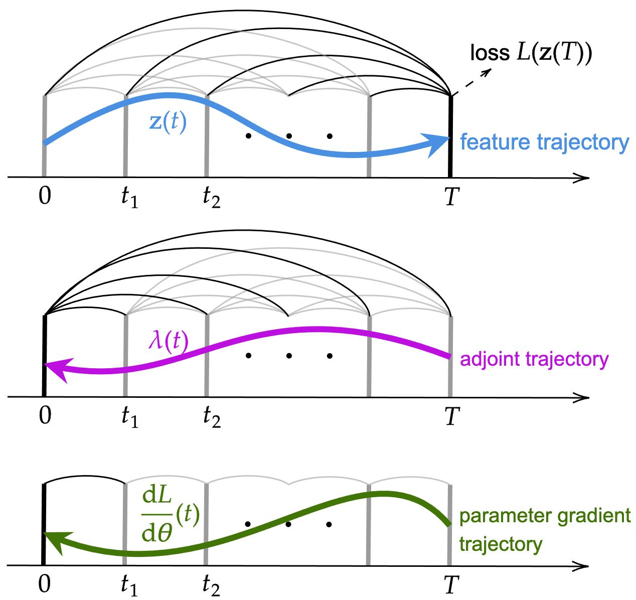
Figure 1: The visualization of the adjoint backpropagation method for training neural FDEs by solving an augmented FDE backward in time.

4.4 Model Complexity

During the forward pass, as described in ˜9, the process requires computing the fractional derivative $f(t_{k},\mathbf{z}_{k};\bm{\theta})$ at each iteration, with results stored in memory for subsequent steps. The total time complexity over the entire process can be expressed as $\sum_{k=0}^{N}(C+O(k))$, where $O(k)$ represents the computational overhead of summing and weighting the $k$ terms at each step. Here, $N=\frac{T}{h}$ denotes the number of discretization (iteration) steps necessary for the integration process, and $C$ indicates the computational complexity of the function $f$. This leads to a total cost of $O(NC+N^{2})$. With a fast algorithm for the convolution computations, we generally need $O(N\log(N))$ for the convolution (Mathieu, Henaff, and LeCun 2013), resulting in $O(NC+N\log(N))$. The memory complexity is represented by $O(P+Nd)$, where $d$ indicates the memory requirement for each hidden state $\mathbf{z}_{k}$ and $P$ denotes the peak memory usage for computing $f$ at a single timestep. The term $Nd$ arises from storing all fractional derivatives $\{f(t_{j},\mathbf{z}_{j};{\bm{\theta}})\}_{j=1}^{N}$ as described in ˜9, where each value has the same dimension as the state $\mathbf{z}_{k}$.

During the backward phase, as indicated by computations in ˜18 and 19, a sequence of vector-Jacobian products is required. According to (Griewank 2003), computing these products demands approximately at most 2 to 3 times the computational time complexity compared to evaluating the original function $f$. The time complexity is again $O(NC+N^{2})$. The computational memory complexity stands at $O(Q+Nd)$, assuming the memory cost for the vector-Jacobian product $\lambda\frac{\partial f}{\partial\bm{\theta}}$ is around $Q$. The term $d$ arises because $\lambda\frac{\partial f}{\partial\mathbf{z}}$ shares the same dimension as the hidden state. For large-dimensional $\bm{\theta}$, the gradient memory requirement for $\lambda\frac{\partial f}{\partial\bm{\theta}}$ may be the dominant one since the dimension of $\bm{\theta}$ typically exceeds that of the hidden state $\mathbf{z}_{k}$ in practical implementations.

Direct differentiation through the forward iterations ˜9 requires storing both intermediate states and their gradients with respect to all model parameters at each time step since the computation involves all values from past time steps with a dense connection pattern. This is essential for calculating gradients by applying the chain rule throughout the intermediate computations. The memory requirement increases to at least $O(NQ+Nd)$ assuming the gradient memory requirement at each time step is around $Q$, thereby exceeding $O(Q+Nd)$ required by our adjoint method.

A final note is that the memory requirement $O(Nd)$ for storing all fractional derivatives $\{f(t_{j},\mathbf{z}_{j};{\bm{\theta}})\}_{j=1}^{N}$ can be reduced to $KO(d)$ by using the short memory principle (Deng 2007; Podlubny 1999) to modify the summation in ˜18 to $\sum^{N-k+K-1}_{j=N-k}$. This approximation corresponds to using a shifting memory window with a fixed width $K$ rather than the full history. The diagram is shown in (Kang et al. 2024a)[Figure 1].

Model MLP Node2vec GCN GraphSAGE GRAND-l F-GRAND-l F-GRAND-nl adj-F-GRAND-l adj-F-GRAND-nl Accuracy 61.06$\pm$0.08 72.49$\pm$0.10 75.64$\pm$0.21 78.29$\pm$0.16 75.56$\pm$0.67 77.25$\pm$0.62 77.01$\pm$0.22 78.36$\pm$0.32 78.33$\pm$0.20

Table 2: Node classification accuracy(%) on Ogbn-products dataset. The best and the second-best results for each criterion are highlighted in bold and underlined, respectively.

5 Experiments

To evaluate the efficiency of our neural FDE solvers, experiments were conducted on three tasks: biological system FDE discovery, image classification, and graph node classification. The experiments in this section are designed to achieve two main objectives: 1) To verify that our adjoint FDE training accurately computes gradients and supports backpropagation. This is demonstrated in the small-scale problem described in Section˜5.1, where the estimated parameters are shown to converge to the ground-truth values following the adjoint gradients. 2) To show that our adjoint FDE training is memory-efficient for large-scale problems. Experiments in Sections˜5.2 and 5.3, particularly with the large-scale Ogbn-Products dataset, support this claim. It is important to note that our primary goal is to showcase the efficiency of the proposed adjoint backpropagation method for training neural FDEs by solving the augmented FDE backward in time, rather than achieving state-of-the-art results. Our empirical tests demonstrate that this approximation not only reduces the computational memory required for training but also maintains reasonable performance across various experimental setups. The experiments were conducted on a workstation running Ubuntu 20.04.1, equipped with an AMD Ryzen Threadripper PRO 3975WX with 32 cores and an NVIDIA RTX A5000 GPU with 24GB of memory.

5.1 Fractional Lotka-Volterra Model

We consider a nonlinear fractional Lotka-Volterra system, comprising two differential equations that describe the dynamics of biological systems where two species interact, one as a predator and the other as a prey:

$$\begin{aligned} &{}_{\mathrm{left}}D_{C}^{\beta}x=x(a-cy),\\ &{}_{\mathrm{left}}D_{C}^{\beta}y=-y(b-dx),\end{aligned}$$

where $x$ and $y$ represent prey and predator populations, respectively, and $a,b,c,d$ are constants indicating interaction dynamics. We set the ground truth parameters as $[a,b,c,d]=[1.0,0.5,1.0,0.3]$. Using synthetic data generated with these parameters and initial conditions randomly selected from $[0.5,5]$, we train a model to estimate the parameters. The model uses the Adam optimizer (Kingma and Ba 2014) with a learning rate of 0.01. After 30 epochs, the estimated parameters, $[0.99,0.48,1.05,0.33]$, closely match the true values, demonstrating the efficiency of our adjoint backpropagation. We do not validate the gradient in high-dimensional cases because these scenarios have many local minima, and there is no guarantee of achieving the global minimum.

Method Test Error Train. GPU Mem (MB) Training Time (s) Inf. GPU Mem (MB) Inference Time (s) Direct 0.39% 3612 1.46 1628 0.54 Adjoint 0.36% 2432 1.41 1628 0.54

Table 3: Comparative performance of direct differentiation vs. adjoint backpropagation on the MNIST dataset with $T=20$.

$T$ 1 5 10 20 30 40 50 60 70 100 200 $\text{M}_{\mathrm{dir}}$ 1.8 2.2 2.7 3.6 4.6 5.5 6.5 7.4 8.4 11.2 20.7 $\text{M}_{\mathrm{adj}}$ 1.8 1.9 2.1 2.4 2.5 2.9 3.2 3.5 3.9 5.0 8.4 $\frac{\text{M}_{\mathrm{adj}}}{\text{M}_{\mathrm{dir}}}$ 1.00 0.88 0.79 0.67 0.55 0.51 0.49 0.48 0.46 0.44 0.40

Table 4: GPU memory usage (GB) during training on the MNIST dataset across different integral times $T$. Notations $\text{M}_{\mathrm{dir}}$ and $\text{M}_{\mathrm{adj}}$ represent the memory usage using the direct differentiation and the adjoint backpropagation. The ration $\frac{\text{M}_{\mathrm{adj}}}{\text{M}_{\mathrm{dir}}}$ quantifies the relative memory consumption between the two methods.

5.2 Image Classification

This experiment evaluates the performance of neural FDEs on the MNIST dataset (LeCun et al. 1998), with a focus on comparing the adjoint backpropagation to the direct differentiation through forward-pass iterations. The aim is to assess the models in terms of both accuracy and computational cost. Following the model architecture from (Chen et al. 2018), the input is downsampled twice. The model’s hidden features are then updated following a neural FDE. Here, $f(t,\mathbf{z}(t);\bm{\theta})$ is configured as a convolution module. The step size $h$ is set to $0.1$, and the fractional order $\beta$ is set to $0.5$. This configuration implies a continuous analog to discrete layer indices in traditional neural networks, corresponding to approximately $N=T/h$ layers. Subsequently, a fully connected layer is applied to the extracted features for classification. In both the training and testing phases, the batch size is set to 128. In the first setting, gradients are backpropagated directly through forward-pass operations in ˜9, while in the second setting, we solve the proposed reverse-mode FDE in Section˜4.3 to obtain the gradients.

The model’s test accuracy, along with training and testing memory and time, are presented in Table˜3 when $T=20$. Both training methods achieve an accuracy of over 99.5%. Comparing the training memory, we find that training neural FDEs by solving the augmented FDE backward reduces memory usage by nearly 33% in this setting. Furthermore, we set integral times $T$ ranging from 1 to 200 and record the GPU memory usage in Table˜4. We observe that with sufficiently large $T$, the adjoint backpropagation consumes only 40% of the training memory compared to the direct differentiation.

Model adj-F- GRAND-l F-GRAND-l adj-F- GRAND-nl F-GRAND-nl Inference Time (s) 0.102 0.102 0.185 0.185 Inf. GPU Mem. (MB) 3982 3982 4314 4314 Training Time (s) 0.319 0.352 0.785 0.806 Train. GPU Mem. (MB) 5570 8527 9086 18180

Table 5: Computation cost of models on the Ogbn-arxiv dataset: integral time $T=10$ and step size of 1.

Model adj-F- GRAND-l F-GRAND-l adj-F- GRAND-nl F-GRAND-nl Inference Time (s) 34.39 34.39 36.11 36.11 Inf. GPU Mem. (MB) 2678 2678 4468 4468 Training Time (s) 34.04 35.15 43.24 44.41 Train. GPU Mem. (MB) 6602 7950 11238 17210

Table 6: Computation cost of models on the Ogbn-products dataset: integral time $T=10$ and step size of 1.

5.3 Node Classification on Graph Dataset

In this section, we validate the efficiency of our neural FDE solvers through experiments conducted across a range of graph node classification tasks, as outlined in (Kang et al. 2024a). These experiments utilize the neural FDE model F-GRAND, detailed in (Kang et al. 2024a)[Sec. 3.1.1]. It includes two variants, F-GRAND-nl and F-GRAND-l, denoting nonlinear and linear graph feature dynamics $f$, respectively. Utilizing our neural FDE toolbox, we aim to demonstrate that our solver can match the performance of traditional solvers (Kang et al. 2024a) that rely on the direct differentiation using PyTorch without using the adjoint backpropagation method. Models trained using our adjoint backpropagation technique are prefixed with adj-. Moreover, we show that our neural FDE toolbox significantly reduces computational memory demand during training.

We follow the experimental setup from GRAND (Chamberlain et al. 2021), conducting experiments on homophilic datasets. We adopt the same dataset splitting method as in (Chamberlain et al. 2021), using the Largest Connected Component (LCC) and performing random splits. For the Ogbn-products dataset, we employ a mini-batch training approach as outlined in the paper (Zeng et al. 2020). For detailed information on the dataset and implementation specifics, please refer to the Appendix.

From Table˜1, we observe that our adjoint backpropagation delivers comparable performance across all datasets on node classification tasks. This demonstrates the effectiveness of our proposed gradient computation using the proposed reverse-mode FDE. Furthermore, Table˜2 includes the large-scale Ogbn-Products dataset, with 2449029 nodes and 61859140 edges. The memory efficiency of adj-F-GRAND enables the use of larger batch sizes, which contributes to improved classification outcomes. In our experiments, the batch size for adj-F-GRAND is set to 20,000 compared to 10,000 for F-GRAND when executed on the same GPU. Setting the F-GRAND batch size to 20000, however, leads to Out-Of-Memory (OOM) errors.

We also investigate the computational memory costs associated with these training methods with the other settings all the same. From Table˜5 and Table˜6, it is evident that our adjoint solvers significantly reduce computational memory costs during the training phase for the same model. Especially for the GRAND-nl model, which recomputes the attention score at each integration step, our adjoint solvers require only half the memory compared to traditional solvers. This highlights the remarkable efficiency of our adjoint method.

6 Conclusion

In this paper, we propose an efficient neural FDE training strategy by solving an augmented FDE backward in time, which substantially reduces memory requirements. Our approach provides a practical neural FDE toolbox and holds considerable promise for diverse applications. We demonstrate the effectiveness of our solver in image classification, biological system FDE discovery, and graph node classification. Our training using the adjoint backpropagation can perform comparably to baseline models while significantly reducing computational overhead. The new neural FDE training technique will benefit the community by enabling more efficient use of computational resources and has the potential to scale to large FDE systems.

This supplementary document complements the main paper by providing comprehensive details and supporting evidence necessary for a full understanding of the research conducted. The sections are organized as follows:

1. A detailed exposition on the derivation of the adjoint method is provided in Appendix˜A. This section outlines the theoretical underpinnings and computational efficiencies gained through our approach, enhancing the reader’s grasp of our method.

2. The experimental design and dataset specifics are extensively covered in Appendix˜B. This includes a detailed breakdown of dataset characteristics, preprocessing steps, and experimental setups.

3. We discuss the limitations of our work and discuss its broader impact in Appendix˜C.

4. Lastly, the entire codebase used in our research is made available. This includes the implementation of the adjoint backpropagation technique within the torchfde toolbox, available at https://github.com/kangqiyu/torchfde.

Appendix A Neural FDE and Adjoint Backpropagation

In the main paper Section˜4.2, we sketch the derivation of the adjoint method which is an effective strategy for training the neural FDE by utilizing an augmented FDE in the reverse direction. In this section, we present the full derivation with more discussions.

Consider a scalar-valued loss function $L(\cdot)$ that depends on the terminal state $\mathbf{z}(T)$. Our primary goal is to minimize $L(\mathbf{z}(T))$ with respect to $\bm{\theta}$. We need to compute the gradient $\frac{\mathrm{d}{L\left(\mathbf{z}(T)\right)}}{\mathrm{d}{\bm{\theta}}}$ for gradient descent. The strategy is to find a Lagrangian function $\lambda(t)$ to circumvent the direct computation of challenging derivatives such as $\frac{\mathrm{d}{\mathbf{z}(T)}}{\mathrm{d}{\bm{\theta}}}$ or $\frac{\mathrm{d}{\mathbf{z}(t)}}{\mathrm{d}{\bm{\theta}}}$. To this end, we consider the following optimization problem:

$$\begin{aligned} \min_{\bm{\theta}}\quad&L\left(\mathbf{z}\left(T\right)\right)\\ \text{subject to}\quad&\begin{aligned} &F\left({}_{\mathrm{left}}D_{C}^{\beta}\mathbf{z}(t),\mathbf{z}(t),\bm{\theta},t\right)\\ &\quad\quad\coloneqq{}_{\mathrm{left}}D_{C}^{\beta}\mathbf{z}(t)-f(t,\mathbf{z}(t);\bm{\theta})=0\\ &\text{for all }t\in[0,T],\end{aligned}\\ &\mathbf{z}\left(0\right)=\mathbf{z}_{0}.\end{aligned}$$ (20)

We define the augmented objective function $\psi$ as

$$\psi=L\left(\mathbf{z}\left(T\right)\right)-\int_{0}^{T}\lambda(t)F\left({}_{\mathrm{left}}D_{C}^{\beta}\mathbf{z}(t),\mathbf{z}(t),\bm{\theta},t\right)\,\mathrm{d}t.$$ (21)

Since $F\left({}_{\mathrm{left}}D_{C}^{\beta}\mathbf{z}(t),\mathbf{z}(t),\bm{\theta},t\right)=0$ for all $t\in[0,T]$, the derivative $\frac{\mathrm{d}{L\left(\mathbf{z}(T)\right)}}{\mathrm{d}{\bm{\theta}}}$ is the same as $\frac{\mathrm{d}{\psi}}{\mathrm{d}{\bm{\theta}}}$.

For the second term on the right-hand side of ˜21, we have

$$\int_{0}^{T}\lambda(t)F\,\mathrm{d}t$$

$$=\int_{0}^{T}\lambda(t)({}_{\mathrm{left}}D_{C}^{\beta}\mathbf{z}(t)-f(t,\mathbf{z}(t);\bm{\theta}))\,\mathrm{d}t$$

$$=\int_{0}^{T}\lambda(t){}_{\mathrm{left}}D_{C}^{\beta}\mathbf{z}(t)\,\mathrm{d}t-\int_{0}^{T}\lambda(t)f(t,\mathbf{z}(t);\bm{\theta})\,\mathrm{d}t.$$ (22)

For the first term in ˜22, we have

$$\int_{0}^{T}\lambda(t){}_{\mathrm{left}}D_{C}^{\beta}\mathbf{z}(t))\,\mathrm{d}t$$

$$=\frac{1}{\Gamma(1-\beta)}\int_{0}^{T}\lambda(t)\int_{0}^{t}\dot{\mathbf{z}}(u)(t-u)^{-\beta}\mathrm{d}u\,\mathrm{d}t$$

$$=\frac{1}{\Gamma(1-\beta)}\int_{0}^{T}\dot{\mathbf{z}}(u)\int_{u}^{T}\lambda(t)(t-u)^{-\beta}\,\mathrm{d}t\,\mathrm{d}u$$

$$=\frac{1}{\Gamma(1-\beta)}\left.\mathbf{z}(u)\left(\int_{u}^{T}\lambda(t)(t-u)^{-\beta}dt\right)\right|_{0}^{T}$$

$$\quad\quad-\frac{1}{\Gamma(1-\beta)}\int_{0}^{T}\mathbf{z}(u)\frac{\,\mathrm{d}}{\,\mathrm{d}u}\left(\int_{u}^{T}\lambda(t)(t-u)^{-\beta}\,\mathrm{d}t\right)\,\mathrm{d}u$$

$$=-\frac{\mathbf{z}(0)}{\Gamma(1-\beta)}\int_{0}^{T}\lambda(t)t^{-\beta}\,\mathrm{d}t$$

$$\quad\quad-\frac{1}{\Gamma(1-\beta)}\int_{0}^{T}\mathbf{z}(u)\frac{\,\mathrm{d}}{\,\mathrm{d}u}\left(\int_{u}^{T}\lambda(t)(t-u)^{-\beta}\,\mathrm{d}t\right)\,\mathrm{d}u$$

$$=-\frac{\mathbf{z}(0)}{\Gamma(1-\beta)}\int_{0}^{T}\lambda(t)t^{-\beta}\,\mathrm{d}t+\int_{0}^{T}\mathbf{z}(u){}_{\mathrm{right}}D_{\mathrm{RL}}^{\beta}\lambda(u)\,\mathrm{d}u$$

$$=-\frac{\mathbf{z}(0)}{\Gamma(1-\beta)}\int_{0}^{T}\lambda(t)t^{-\beta}\,\mathrm{d}t$$

$$\quad\quad+\int_{0}^{T}\left({}_{\mathrm{right}}D_{C}^{\beta}\lambda(u)+\frac{(T-u)^{-\beta}}{\Gamma(1-\beta)}\lambda(T)\right)\mathbf{z}(u)\,\mathrm{d}u$$

$$=-\frac{\mathbf{z}(0)}{\Gamma(1-\beta)}\int_{0}^{T}\lambda(t)t^{-\beta}\,\mathrm{d}t+\frac{\lambda(T)\int_{0}^{T}\mathbf{z}(u)(T-u)^{-\beta}\,\mathrm{d}u}{\Gamma(1-\beta)}$$

$$\quad\quad+\int_{0}^{T}{}_{\mathrm{right}}D_{C}^{\beta}\lambda(u)\cdot\mathbf{z}(u)\,\mathrm{d}u$$

$$=\lambda(T)J_{\mathrm{left}}^{1-\beta}\mathbf{z}(T)-\mathbf{z}(0)J_{\mathrm{right}}^{1-\beta}\lambda(0)$$

$$\quad\quad+\int_{0}^{T}{}_{\mathrm{right}}D_{C}^{\beta}\lambda(u)\cdot\mathbf{z}(u)\,\mathrm{d}u.$$

Combining ˜21 with the above results, we derive:

$$\begin{aligned} \int_{0}^{T}\lambda(t)F\,\mathrm{d}t&=\lambda(T)J_{\mathrm{left}}^{1-\beta}\mathbf{z}(T)-\mathbf{z}(0)J_{\mathrm{right}}^{1-\beta}\lambda(0)\\ &\hskip-25.6073pt+\int_{0}^{T}{}_{\mathrm{right}}D_{C}^{\beta}\lambda(t)\mathbf{z}(t)\,\mathrm{d}t-\int_{0}^{T}\lambda f(t,\mathbf{z}(t);\bm{\theta})\,\mathrm{d}t.\end{aligned}$$

Take the derivative with respect to $\bm{\theta}$, we have

$$\begin{aligned} \frac{\mathrm{d}}{\mathrm{d}\bm{\theta}}\left[\int_{0}^{T}\lambda F\,\mathrm{d}t\right]&=\lambda\left(T\right)\frac{\mathrm{d}J_{\mathrm{left}}^{1-\beta}\mathbf{z}(T)}{\mathrm{d}\bm{\theta}}-J_{\mathrm{right}}^{1-\beta}\lambda(0)\frac{\mathrm{d}\mathbf{z}(0)}{\mathrm{d}\bm{\theta}}\\ &+\int_{0}^{T}\left(\frac{\mathrm{d}{\mathbf{z}}}{\mathrm{d}{\bm{\theta}}}{}_{\mathrm{right}}D_{C}^{\beta}\lambda(t)-\lambda\frac{\mathrm{d}f}{\mathrm{d}\bm{\theta}}\right)\,\mathrm{d}t.\end{aligned}$$

Since $\mathbf{z}_{0}$ is the initial input hidden feature of the neural FDE, we have $\frac{\mathrm{d}\mathbf{z}(0)}{\mathrm{d}\bm{\theta}}=0$. Applying the chain rule, we get $\frac{\mathrm{d}f}{\mathrm{d}\bm{\theta}}=\frac{\partial f}{\partial\bm{\theta}}+\frac{\partial f}{\partial\mathbf{z}}\frac{\mathrm{d}{\mathbf{z}}}{\mathrm{d}{\bm{\theta}}}$. Consequently, the derivative of the integral expression is given by:

$$\begin{aligned} &\frac{\mathrm{d}}{\mathrm{d}\bm{\theta}}\left[\int_{0}^{T}\lambda F\,\mathrm{d}t\right]=\lambda\left(T\right)\frac{\mathrm{d}J_{\mathrm{left}}^{1-\beta}\mathbf{z}(T)}{\mathrm{d}\bm{\theta}}\\ &\quad+\int_{0}^{T}\left({}_{\mathrm{right}}D_{C}^{\beta}\lambda(t)-\lambda(t)\frac{\partial f}{\partial\mathbf{z}}\right)\frac{\mathrm{d}{\mathbf{z}}}{\mathrm{d}{\bm{\theta}}}\,\mathrm{d}t-\int_{0}^{T}\lambda\frac{\partial f}{\partial\bm{\theta}}\,\mathrm{d}t.\end{aligned}$$ (23)

It follows that

$$\frac{\mathrm{d}L}{\mathrm{d}\bm{\theta}}=\frac{\,\mathrm{d}L}{\,\mathrm{d}J_{\mathrm{left}}^{1-\beta}\mathbf{z}(T)}\frac{\mathrm{d}J_{\mathrm{left}}^{1-\beta}\mathbf{z}(T)}{\mathrm{d}\bm{\theta}}-\frac{\mathrm{d}}{\mathrm{d}\bm{\theta}}\left[\int_{0}^{T}\lambda F\,\mathrm{d}t\right]$$

$$=\frac{\,\mathrm{d}L}{\,\mathrm{d}J_{\mathrm{left}}^{1-\beta}\mathbf{z}(T)}\frac{\mathrm{d}J_{\mathrm{left}}^{1-\beta}\mathbf{z}(T)}{\mathrm{d}\bm{\theta}}-\lambda\left(T\right)\frac{\mathrm{d}J_{\mathrm{left}}^{1-\beta}\mathbf{z}(T)}{\mathrm{d}\bm{\theta}}$$

$$-\int_{0}^{T}\left({}_{\mathrm{right}}D_{C}^{\beta}\lambda(t)-\lambda(t)\frac{\partial f}{\partial\mathbf{z}}\right)\frac{\mathrm{d}{\mathbf{z}}}{\mathrm{d}{\bm{\theta}}}\,\mathrm{d}t+\int_{0}^{T}\lambda\frac{\partial f}{\partial\bm{\theta}}\,\mathrm{d}t$$

$$=\left(\frac{\,\mathrm{d}L}{\,\mathrm{d}J_{\mathrm{left}}^{1-\beta}\mathbf{z}(T)}-\lambda\left(T\right)\right)\frac{\mathrm{d}J_{\mathrm{left}}^{1-\beta}\mathbf{z}(T)}{\mathrm{d}\bm{\theta}}$$

$$-\int_{0}^{T}\left({}_{\mathrm{right}}D_{C}^{\beta}\lambda(t)-\lambda(t)\frac{\partial f}{\partial\mathbf{z}}\right)\frac{\mathrm{d}{\mathbf{z}}}{\mathrm{d}{\bm{\theta}}}\,\mathrm{d}t+\int_{0}^{T}\lambda\frac{\partial f}{\partial\bm{\theta}}\,\mathrm{d}t.$$ (24)

To avoid the direct computation of challenging derivatives such as $\frac{\mathrm{d}{\mathbf{z}(T)}}{\mathrm{d}{\bm{\theta}}}$ or $\frac{\mathrm{d}{\mathbf{z}(t)}}{\mathrm{d}{\bm{\theta}}}$, we let $\lambda(t)$ satisfy the following FDE:

$$\begin{aligned} {}_{\mathrm{right}}D_{C}^{\beta}\lambda(t)&=\lambda(t)\frac{\partial f}{\partial\mathbf{z}},\\ \text{ with }\lambda\left(T\right)&=\frac{\,\mathrm{d}L}{\,\mathrm{d}J_{\mathrm{left}}^{1-\beta}\mathbf{z}(T)}.\end{aligned}$$ (25)

Consequently, as the first two terms in ˜24 vanish, we obtain

$$\frac{\mathrm{d}L}{\mathrm{d}\bm{\theta}}=-\int_{T}^{0}\lambda(t)\frac{\partial f}{\partial\bm{\theta}}\,\mathrm{d}t.$$ (26)

To facilitate computation, we approximate the constraint on the last time point as $\frac{\,\mathrm{d}L}{\,\mathrm{d}J_{\mathrm{left}}^{1-\beta}\mathbf{z}(T)}\approx\frac{\,\mathrm{d}L}{\,\mathrm{d}\mathbf{z}(T)}$ in ˜25. This approximation represents the gradient of the loss with respect to the final state of the system. Efficient evaluation of the vector-Jacobian products, $\lambda(t)\frac{\partial f}{\partial\mathbf{z}}$ and $\lambda(t)\frac{\partial f}{\partial\bm{\theta}}$, specified in ˜25 and ˜26, is achieved using automatic differentiation, offering a computational cost on par with that of evaluating $f$ directly.

In the reverse model, the systems described in ˜25 and 26 are computed simultaneously. Echoing the methodologies employed in ˜9 and 10, we utilize standard quadrature techniques to solve these equations. Our numerical iterations confirm that the coefficients are consistent with those reported in ˜9 and 10. Additionally, the trajectory $\mathbf{z}(t)$ generated during the forward pass can be efficiently reused.

Setting $\beta=1$ simplifies the FDE described in ˜15 into a first-order neural ODE. This transformation aligns the computation of the reverse model FDE with the first-order neural ODE framework utilized in (Chen et al. 2018). It can be formulated in summary as

$$\begin{aligned} \frac{\,\mathrm{d}}{\,\mathrm{d}t}\lambda(t)&=\lambda(t)\frac{\partial f}{\partial\mathbf{z}},\\ \frac{{\mathrm{d}L}/{\mathrm{d}\bm{\theta}}}{\,\mathrm{d}t}&=\lambda(t)\frac{\partial f}{\partial\bm{\theta}},\end{aligned}$$ (27)

with $\lambda(T)=\frac{\,\mathrm{d}L}{\,\mathrm{d}\mathbf{z}(T)}$ and $\frac{\,\mathrm{d}L}{\,\mathrm{d}\bm{\theta}}(T)=\mathbf{0}_{|\bm{\theta}|}$.

Dataset	Type	Classes	Features	Nodes	Edges
Cora	citation	7	1433	2485	5069
Citeseer	citation	6	3703	2120	3679
PubMed	citation	3	500	19717	44324
Coauthor CS	co-author	15	6805	18333	81894
Computers	co-purchase	10	767	13381	245778
Photos	co-purchase	8	745	7487	119043
CoauthorPhy	co-author	5	8415	34493	247962
OGB-Arxiv	citation	40	128	169343	1166243
OGB-Products	co-purchase	47	100	2449029	61859140

Table 7: Dataset Statistics used in Tables˜1 and 6.

Appendix B Datasets and Experiments Setting

B.1 Graph Datasets Used in the Main Paper

To validate the efficiency of our neural FDE solvers, experiments in Section˜5.3 were performed in a range of graph learning tasks. The dataset statistics used in Tables˜1 and 6 are provided in Table˜7. Following the experimental framework in (Chamberlain et al. 2021), we select the largest connected component from each dataset.

Dataset	lr	weight decay	indrop	dropout	hidden dim	time	step size
Cora	0.005	0.0001	0.4	0.2	80	4	0.2
Citeseer	0.001	0.0001	0.4	0.4	64	4	1
PubMed	0.001	0.0001	0.2	0.4	64	10	0.2
Coauthor CS	0.005	0.0001	0.4	0.4	8	8	1
Computers	0.005	0.0001	0.2	0.4	64	3	0.5
Photos	0.001	0.0001	0.2	0.4	128	4	0.2
CoauthorPhy	0.005	0.0001	0.2	0.4	64	4	0.5
OGB-Arxiv	0.005	0.0001	0.4	0.2	128	8	0.2
OGB-Products	0.001	0.0001	0.2	0.4	128	10	0.2

Table 8: Hyper-parameters used in Table˜1

B.2 Hyper-parameters

We utilized a grid search approach on the validation dataset to fine-tune common hyperparameters including hidden dimensions, learning rate, weight decay, and dropout rate. The specific hyperparameters utilized in Table˜1 are detailed in Table˜8. For a comprehensive understanding of the hyperparameter configurations, we direct readers to the accompanying codebase in the supplementary material, which includes the provided code for reproducibility.

$T$	1	10	20	30	40	50	60	70	100	170
Direct	1600	2692	3906	5122	6336	7532	8746	9962	13606	22072
Adjoint	1552	1818	2166	2510	2854	3178	3526	3870	4906	7298
$\frac{\text{Adjoint}}{\text{Direct}}$	0.97	0.68	0.55	0.49	0.45	0.42	0.40	0.39	0.36	0.33

Table 9: GPU memory usage (MB) during training on the Fashion-MNIST dataset across various integral times $T$ with $h=0.1$.

B.3 More Experiments on Image Dataset

This supplementary document extends the adjoint backpropagation evaluation of neural FDEs on the MNIST dataset (LeCun et al. 1998), initially presented in Section˜5.2 of the main paper, to the Fashion-MNIST dataset (Xiao, Rasul, and Vollgraf 2017). Fashion-MNIST consists of 28$\times$28 grayscale images of 70,000 fashion items across 10 categories, with each category containing 7,000 images. It mirrors MNIST in image size, data format, and the structure of training and testing splits, featuring 60,000 images in the training set and 10,000 in the test set. In our experiments, the model’s hidden features are updated using a neural FDE where $f(t,\mathbf{z}(t);\bm{\theta})$ is implemented as a convolution module. The step size $h$ is set at 0.1, and the fractional order $\beta$ at 0.3. Batch sizes of 128 are used during both the training and testing phases. In the first setting, the gradients are backpropagated directly through forward-pass operations in ˜9, while in the second setting, we solve the proposed reverse-mode FDE in Section˜4.3 to obtain the gradients. When $T=1$, we find training with the adjoint backpropagation achieves a test accuracy of over 92.05% while training with the direct differentiation achieves 92.35%. Furthermore, we set integral times $T$ ranging from 1 to 170 and record the GPU memory usage in Table˜9. We observe that with sufficiently large $T$, the adjoint backpropagation consumes only 33% of the training memory compared to the direct differentiation. Additionally, we observe that the GPU memory during training scales linearly with the integration time $T$ with a fixed step size $h$. This meets our complexity analysis in Section˜4.4.

Appendix C Limitations and Broader Impact

While the proposed scalable adjoint backpropagation method for training neural FDEs introduces significant improvements in memory efficiency and computational overhead, there are several limitations that merit attention. For instance, this method may introduce numerical inaccuracies due to interpolation errors and sensitivity to initial conditions when solving the augmented FDE backward in time. This sensitivity could impact the robustness and generalizability of the models trained using this method, particularly in chaotic FDE systems. The integration of fractional-order calculus with deep learning opens new possibilities for modeling complex dynamical systems with greater accuracy and flexibility than traditional integer-order models. This advancement has broad implications across various fields. For example, enhanced modeling capabilities could lead to more precise simulations and predictions in physics, biology, and engineering, facilitating breakthroughs in understanding complex systems. Additionally, by reducing computational requirements, smaller organizations and researchers with limited resources may also leverage advanced models, potentially democratizing access to cutting-edge AI tools.

References

- Abadi et al. (2016) Abadi, M.; Barham, P.; Chen, J.; Chen, Z.; Davis, A.; Dean, J.; Devin, M.; Ghemawat, S.; Irving, G.; Isard, M.; et al. 2016. TensorFlow: a system for Large-Scale machine learning. In 12th USENIX symposium on operating systems design and implementation (OSDI 16), 265–283.
- Almeida, Bastos, and Monteiro (2016) Almeida, R.; Bastos, N. R.; and Monteiro, M. T. T. 2016. Modeling some real phenomena by fractional differential equations. Mathematical Methods in the Applied Sciences, 39(16): 4846–4855.
- Anastasio (1994) Anastasio, T. J. 1994. The fractional-order dynamics of brainstem vestibulo-oculomotor neurons. Biological cybernetics, 72(1): 69–79.
- Antil et al. (2020) Antil, H.; Khatri, R.; Löhner, R.; and Verma, D. 2020. Fractional deep neural network via constrained optimization. Mach. Learn.: Sci. Technol., 2(1): 015003.
- Brunton, Proctor, and Kutz (2016) Brunton, S. L.; Proctor, J. L.; and Kutz, J. N. 2016. Discovering governing equations from data by sparse identification of nonlinear dynamical systems. Proceedings of the national academy of sciences, 113(15): 3932–3937.
- Chamberlain et al. (2021) Chamberlain, B. P.; Rowbottom, J.; Goronova, M.; Webb, S.; Rossi, E.; and Bronstein, M. M. 2021. GRAND: Graph Neural Diffusion. In Proc. Int. Conf. Mach. Learn.
- Chami et al. (2019) Chami, I.; Ying, Z.; Ré, C.; and Leskovec, J. 2019. Hyperbolic graph convolutional neural networks. In Advances Neural Inf. Process. Syst.
- Chen et al. (2018) Chen, R. T.; Rubanova, Y.; Bettencourt, J.; and Duvenaud, D. 2018. Neural ordinary differential equations. In Advances Neural Inf. Process. Syst.
- Chen et al. (2021) Chen, Y.; Liu, F.; Yu, Q.; and Li, T. 2021. Review of fractional epidemic models. Applied mathematical modelling, 97: 281–307.
- Coleman and Noll (1961) Coleman, B. D.; and Noll, W. 1961. Foundations of linear viscoelasticity. Rev. Modern Phys., 33(2): 239.
- Cui et al. (2025) Cui, W.; Kang, Q.; Li, X.; Zhao, K.; Tay, W. P.; Deng, W.; and Li, Y. 2025. Neural Variable-Order Fractional Differential Equation Networks. In Proc. AAAI Conference on Artificial Intelligence. Philadelphia, USA.
- Deng (2007) Deng, W. 2007. Short memory principle and a predictor–corrector approach for fractional differential equations. J. Comput. Appl. Math., 206(1): 174–188.
- Diaz-Diaz and Estrada (2022) Diaz-Diaz, F.; and Estrada, E. 2022. Time and space generalized diffusion equation on graph/networks. Chaos, Solitons and Fractals, 156: 111791.
- Diethelm (2010) Diethelm, K. 2010. The analysis of fractional differential equations: an application-oriented exposition using differential operators of Caputo type, volume 2004. Lect. Notes Math.
- Diethelm and Ford (2002) Diethelm, K.; and Ford, N. J. 2002. Analysis of fractional differential equations. J. Math. Anal. Appl., 265(2): 229–248.
- Diethelm and Ford (2009) Diethelm, K.; and Ford, N. J. 2009. Numerical analysis for distributed-order differential equations. J. Comput. Appl. Math., 225(1): 96–104.
- Diethelm, Ford, and Freed (2004) Diethelm, K.; Ford, N. J.; and Freed, A. D. 2004. Detailed error analysis for a fractional Adams method. Numer. Algorithms, 36: 31–52.
- Dupont, Doucet, and Teh (2019) Dupont, E.; Doucet, A.; and Teh, Y. W. 2019. Augmented neural odes. In Advances Neural Inf. Process. Syst., 1–11.
- Gao and Sun (2011) Gao, G.-h.; and Sun, Z.-z. 2011. A compact finite difference scheme for the fractional sub-diffusion equations. Journal of Computational Physics, 230(3): 586–595.
- Gravina, Bacciu, and Gallicchio (2022) Gravina, A.; Bacciu, D.; and Gallicchio, C. 2022. Anti-symmetric dgn: A stable architecture for deep graph networks. In Proc. Int. Conf. Learn. Representations.
- Griewank (2003) Griewank, A. 2003. A mathematical view of automatic differentiation. Acta Numerica, 12: 321–398.
- Guo et al. (2022) Guo, L.; Wu, H.; Yu, X.; and Zhou, T. 2022. Monte Carlo fPINNs: Deep learning method for forward and inverse problems involving high dimensional fractional partial differential equations. Comput. Methods Appl. Mechanics Eng., 400: 115523.
- Haber and Ruthotto (2017) Haber, E.; and Ruthotto, L. 2017. Stable architectures for deep neural networks. Inverse Problems, 34(1): 1–23.
- Ionescu et al. (2017) Ionescu, C.; Lopes, A.; Copot, D.; Machado, J. T.; and Bates, J. H. 2017. The role of fractional calculus in modeling biological phenomena: A review. Commun. Nonlinear Sci. Numer. Simul., 51: 141–159.
- Javadi et al. (2023) Javadi, R.; Mesgarani, H.; Nikan, O.; and Avazzadeh, Z. 2023. Solving Fractional Order Differential Equations by Using Fractional Radial Basis Function Neural Network. Symmetry, 15(6): 1275.
- Ji et al. (2021) Ji, W.; Qiu, W.; Shi, Z.; Pan, S.; and Deng, S. 2021. Stiff-pinn: Physics-informed neural network for stiff chemical kinetics. The Journal of Physical Chemistry A, 125(36): 8098–8106.
- Kaczorek and Rogowski (2015) Kaczorek, T.; and Rogowski, K. 2015. Fractional linear systems and electrical circuits. Springer.
- Kang et al. (2021) Kang, Q.; Song, Y.; Ding, Q.; and Tay, W. P. 2021. Stable neural ode with Lyapunov-stable equilibrium points for defending against adversarial attacks. Advances in Neural Information Processing Systems, 34: 14925–14937.
- Kang et al. (2024a) Kang, Q.; Zhao, K.; Ding, Q.; Ji, F.; Li, X.; Liang, W.; Song, Y.; and Tay, W. P. 2024a. Unleashing the Potential of Fractional Calculus in Graph Neural Networks with FROND. In Proc. International Conference on Learning Representations. Vienna, Austria.
- Kang et al. (2024b) Kang, Q.; Zhao, K.; Song, Y.; Xie, Y.; Zhao, Y.; Wang, S.; She, R.; and Tay, W. P. 2024b. Coupling Graph Neural Networks with Fractional Order Continuous Dynamics: A Robustness Study. In Proc. AAAI Conference on Artificial Intelligence. Vancouver, Canada.
- Kaslik and Sivasundaram (2012) Kaslik, E.; and Sivasundaram, S. 2012. Nonlinear dynamics and chaos in fractional-order neural networks. Neural networks, 32: 245–256.
- Kidger, Chen, and Lyons (2021) Kidger, P.; Chen, R. T. Q.; and Lyons, T. J. 2021. "Hey, that’s not an ODE": Faster ODE Adjoints via Seminorms. International Conference on Machine Learning.
- Kingma and Ba (2014) Kingma, D. P.; and Ba, J. 2014. Adam: A method for stochastic optimization. arXiv preprint arXiv:1412.6980.
- Kipf and Welling (2017) Kipf, T. N.; and Welling, M. 2017. Semi-Supervised Classification with Graph Convolutional Networks. In Proc. Int. Conf. Learn. Representations.
- Krapf (2015) Krapf, D. 2015. Mechanisms underlying anomalous diffusion in the plasma membrane. Current Topics Membranes, 75: 167–207.
- Lai et al. (2021) Lai, Z.; Mylonas, C.; Nagarajaiah, S.; and Chatzi, E. 2021. Structural identification with physics-informed neural ordinary differential equations. Journal of Sound and Vibration, 508: 116196.
- LeCun et al. (1998) LeCun, Y.; Bottou, L.; Bengio, Y.; and Haffner, P. 1998. Gradient-based learning applied to document recognition. Proceedings of the IEEE, 86(11): 2278–2324.
- Liu et al. (2022) Liu, Z.; Wang, Y.; Luo, Y.; and Luo, C. 2022. A Regularized Graph Neural Network Based on Approximate Fractional Order Gradients. Mathematics, 10(8): 1320.
- Machado, Kiryakova, and Mainardi (2011) Machado, J. T.; Kiryakova, V.; and Mainardi, F. 2011. Recent history of fractional calculus. Communications in nonlinear science and numerical simulation, 16(3): 1140–1153.
- Mandelbrot and Mandelbrot (1982) Mandelbrot, B. B.; and Mandelbrot, B. B. 1982. The fractal geometry of nature, volume 1. WH freeman New York.
- Mathieu, Henaff, and LeCun (2013) Mathieu, M.; Henaff, M.; and LeCun, Y. 2013. Fast training of convolutional networks through ffts. arXiv preprint arXiv:1312.5851.
- Miyanawala and Jaiman (2017) Miyanawala, T. P.; and Jaiman, R. K. 2017. An efficient deep learning technique for the Navier-Stokes equations: Application to unsteady wake flow dynamics. arXiv preprint arXiv:1710.09099.
- Nigmatullin (1986) Nigmatullin, R. 1986. The realization of the generalized transfer equation in a medium with fractal geometry. Physica status solidi (b), 133(1): 425–430.
- OpenAI (2022) OpenAI. 2022. ChatGPT-4. Available at: https://www.openai.com (Accessed: 10 April 2024).
- Pang, Lu, and Karniadakis (2019) Pang, G.; Lu, L.; and Karniadakis, G. E. 2019. fPINNs: Fractional physics-informed neural networks. SIAM J. Sci. Comput., 41(4): A2603–A2626.
- Paszke et al. (2017) Paszke, A.; Gross, S.; Chintala, S.; Chanan, G.; Yang, E.; DeVito, Z.; Lin, Z.; Desmaison, A.; Antiga, L.; and Lerer, A. 2017. Automatic differentiation in pytorch. In Advances Neural Inf. Process. Syst.
- Paszke et al. (2019) Paszke, A.; Gross, S.; Massa, F.; Lerer, A.; Bradbury, J.; Chanan, G.; Killeen, T.; Lin, Z.; Gimelshein, N.; Antiga, L.; et al. 2019. Pytorch: An imperative style, high-performance deep learning library. Advances in neural information processing systems, 32.
- Podlubny (1994) Podlubny, I. 1994. Fractional-order systems and fractional-order controllers. Institute of Experimental Physics, Slovak Academy of Sciences, Kosice, 12(3): 1–18.
- Podlubny (1999) Podlubny, I. 1999. Fractional Differential Equations. Academic Press.
- Poli et al. (2019) Poli, M.; Massaroli, S.; Park, J.; Yamashita, A.; Asama, H.; and Park, J. 2019. Graph neural ordinary differential equations. arXiv preprint arXiv:1911.07532.
- Pontryagin et al. (1962) Pontryagin, L. S.; Mishchenko, E.; Boltyanskii, V.; and Gamkrelidzem, R. 1962. The Mathematical theory of optimal processes. Routledge.
- Raissi, Perdikaris, and Karniadakis (2019) Raissi, M.; Perdikaris, P.; and Karniadakis, G. E. 2019. Physics-informed neural networks: A deep learning framework for solving forward and inverse problems involving nonlinear partial differential equations. Journal of Computational physics, 378: 686–707.
- Scalas, Gorenflo, and Mainardi (2000) Scalas, E.; Gorenflo, R.; and Mainardi, F. 2000. Fractional calculus and continuous-time finance. Physica A: Statistical Mechanics and its Applications, 284(1-4): 376–384.
- Song et al. (2020) Song, Y.; Sohl-Dickstein, J.; Kingma, D. P.; Kumar, A.; Ermon, S.; and Poole, B. 2020. Score-based generative modeling through stochastic differential equations. arXiv preprint arXiv:2011.13456.
- Sornette (2006) Sornette, D. 2006. Critical phenomena in natural sciences: chaos, fractals, selforganization and disorder: concepts and tools. Springer Science & Business Media.
- Sun and Wu (2006) Sun, Z.-z.; and Wu, X. 2006. A fully discrete difference scheme for a diffusion-wave system. Applied Numerical Mathematics, 56(2): 193–209.
- Tarasov (2011) Tarasov, V. E. 2011. Fractional dynamics: applications of fractional calculus to dynamics of particles, fields and media. Springer Science & Business Media.
- Veličković et al. (2018) Veličković, P.; Cucurull, G.; Casanova, A.; Romero, A.; Liò, P.; and Bengio, Y. 2018. Graph Attention Networks. In Proc. Int. Conf. Learn. Representations, 1–12.
- Wang et al. (2023a) Wang, H.; Fu, T.; Du, Y.; Gao, W.; Huang, K.; Liu, Z.; Chandak, P.; Liu, S.; Van Katwyk, P.; Deac, A.; et al. 2023a. Scientific discovery in the age of artificial intelligence. Nature, 620(7972): 47–60.
- Wang et al. (2023b) Wang, S.; Kang, Q.; She, R.; Tay, W. P.; Hartmannsgruber, A.; and Navarro, D. N. 2023b. RobustLoc: Robust Camera Pose Regression in Challenging Driving Environments. In Proc. AAAI Conference on Artificial Intelligence.
- Wang, Zhang, and Jiang (2022) Wang, S.; Zhang, H.; and Jiang, X. 2022. Fractional physics-informed neural networks for time-fractional phase field models. Nonlinear Dyn., 110(3): 2715–2739.
- Weinan (2017) Weinan, E. 2017. A proposal on machine learning via dynamical systems. Commun. Math. Statist., 1(5): 1–11.
- Xhonneux et al. (2020) Xhonneux; Louis-Pascal; Qu, M.; and Tang, J. 2020. Continuous graph neural networks. In Proc. Int. Conf. Mach. Learn., 10432–10441.
- Xiao, Rasul, and Vollgraf (2017) Xiao, H.; Rasul, K.; and Vollgraf, R. 2017. Fashion-mnist: a novel image dataset for benchmarking machine learning algorithms. arXiv preprint arXiv:1708.07747.
- Yan et al. (2018) Yan, H.; Du, J.; Tan, V. Y.; and Feng, J. 2018. On robustness of neural ordinary differential equations. In Advances Neural Inf. Process. Syst., 1–13.
- Yang et al. (2023) Yang, L.; Zhang, Z.; Song, Y.; Hong, S.; Xu, R.; Zhao, Y.; Zhang, W.; Cui, B.; and Yang, M.-H. 2023. Diffusion models: A comprehensive survey of methods and applications. ACM Computing Surveys, 56(4): 1–39.
- Yu, Perdikaris, and Karniadakis (2016) Yu, Y.; Perdikaris, P.; and Karniadakis, G. E. 2016. Fractional modeling of viscoelasticity in 3D cerebral arteries and aneurysms. Journal of computational physics, 323: 219–242.
- Zeng et al. (2020) Zeng, H.; Zhou, H.; Srivastava, A.; Kannan, R.; and Prasanna, V. 2020. GraphSAINT: Graph Sampling Based Inductive Learning Method. arXiv:1907.04931.
- Zhao et al. (2024) Zhao, K.; Kang, Q.; Ji, F.; Li, X.; Ding, Q.; Zhao, Y.; Liang, W.; and Tay, W. P. 2024. Distributed-Order Fractional Graph Operating Network. In Advances in Neural Information Processing Systems. Vancouver, Canada.