Local models and Bell inequalities for the minimal triangle network

Abstract

Nonlocal correlations created in networks with multiple independent sources enable surprising phenomena in quantum information and quantum foundations. The presence of independent sources, however, makes the analysis of network nonlocality challenging, and even in the simplest nontrivial scenarios a complete characterization is lacking. In this work we study one of the simplest of these scenarios, namely that of distributions invariant under permutations of parties in the minimal triangle network, which features no inputs and binary outcomes. We perform an exhaustive search for triangle-local models, and from it we infer analytic expressions for the boundaries of the set of distributions that admit such models, which we conjecture to be all the tight Bell inequalities for the scenario. Armed with them and with improved outer approximations of the set, we provide new insights on the existence of a classical-quantum gap in the triangle network with binary outcomes.

Bell’s prediction that quantum mechanics should be incompatible with any theory based on local hidden variables [1], later supported by increasingly convincing experiments [2, 3, 4, 5, 6, 7], caused a profound rupture in the conceptual foundations of physics. Gradually, it also became clear that Bell nonlocality [8] is an essential resource for applications in quantum technologies [9, 10], since it allows the certification of nonclassicality of uncharacterized devices [11, 12].

The natural generalization of the scenario considered by Bell are networks [13] where several independent sources distribute physical systems to multiple parties. Network architectures other than those contemplated by Bell scenarios naturally appear, e.g., in quantum communication networks [14] and in schemes for quantum-state transfer [15, 16]. Thus, the characterization of classical and quantum correlations in networks is fundamental to identify quantum advantage in these and other applications. However, the independence of the sources makes these sets of correlations to be non-convex, and thus difficult to characterize. Despite this, many methods have been developed to achieve partial characterizations and develop non-locality witnesses [17, 18, 19, 20, 21] (see also [13]).

Among the possible networks, the triangle network (see Fig. 1a) has received considerable attention, since it is the simplest network where all parties are connected to each other. It is known that it supports genuinely quantum nonlocality [22] and that it is possible to generate in it randomness without needing of measurement choices [23] (as opposed to the Bell scenario where it is known that this is impossible). However, the absence of independences also makes it a challenging scenario to study, even in the simplest case without measurement choices and with binary-valued outcomes. There, the search for realizations is based on brute force [24] (sometimes complemented with the machine learning toolbox [25]), while outer approximations are obtained via inflation methods [19, 26, 27]. Using these tools, it has been discovered that the minimal triangle scenario supports supra-quantum correlations [28], and many witnesses of non-locality have been given [29, 30]. Despite this, the question of whether the binary-outcome triangle network supports quantum but non-classical correlations, posed in Ref. [29], remains open.

(a)

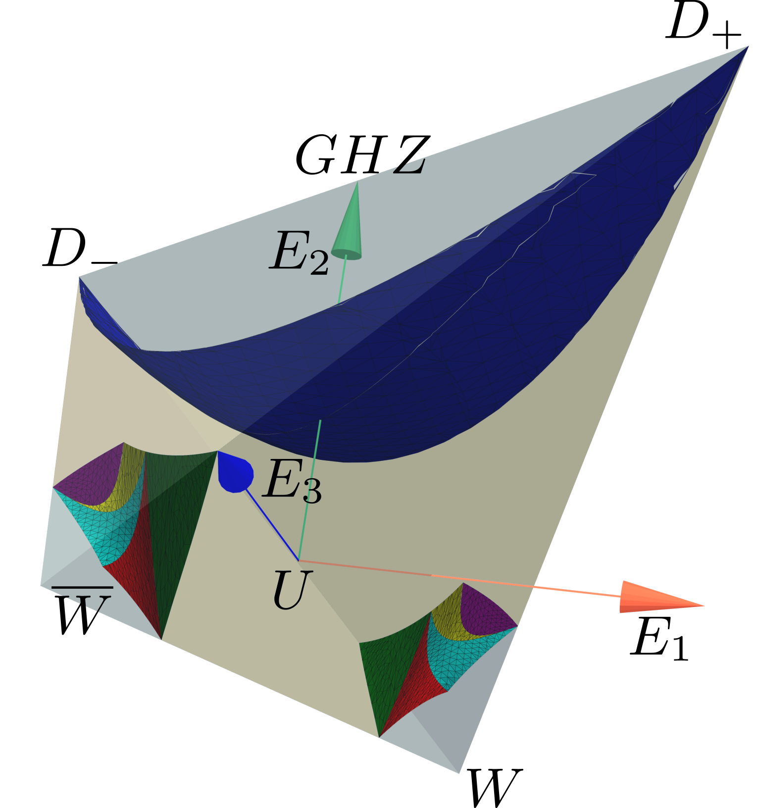
(b)

Figure 1: LABEL:sub@fig:triangle_scenario The minimal triangle scenario. The parties $A$, $B$ and $C$ have no choice of inputs, and their outputs $a$, $b$, $c$ take on values in the set $\left\{-1,1\right\}$. The three sources $\alpha$, $\beta$, and $\gamma$ are assumed to be independent. LABEL:sub@fig:3d A representation in correlator space of the symmetric, network-local distributions that can be generated in the minimal triangle scenario. This figure depicts one of our main contributions, namely an analytic characterization of the coloured boundaries. The distributions $W$, $\overline{W}$, $GHZ$, $D_{+}$, $D_{-}$ and $U$ are defined in the main text.

In this work we perform an exhaustive numerical analysis of the probability distributions symmetric under permutations of parties that can be created in the no-input-binary-outcome triangle network via local hidden variables. This analysis reveals that the upper bound in the cardinality of the hidden variables in Ref. [31] is not needed to achieve a complete characterization of this set of distributions. Moreover, we find analytic expressions for the boundaries of the set. These are polynomial inequalities that, based on the strong numerical evidence built, we conjecture to be the tight Bell inequalities characterizing the scenario, which we depict in Fig. 1b. Armed with them, and with outer approximations based on inflation [19, 26], we provide new insights on the potential existence of a classical-quantum gap in the binary-outcome triangle network: while we shrink some previously known regions candidates to demonstrate quantum nonlocality, we also give new regions where it could be found.

Local correlations in the minimal triangle.—

We consider tripartite statistical behaviors over binary outcomes, $p(a,b,c)$, $a,b,c\in\{-1,1\}$, that are invariant under any relabeling of the parties. These distributions are completely described by the three symmetrized correlators

$$E_{1} = \sum_{a,b,c\in\{-1,1\}}a\,p(a,b,c),$$ (1)

$$E_{2} = \sum_{a,b,c\in\{-1,1\}}ab\,p(a,b,c),$$ (2)

$$E_{3} = \sum_{a,b,c\in\{-1,1\}}abc\,p(a,b,c),$$ (3)

so that the probability distribution is

$$p(a,b,c)=\frac{1}{8}[1+(a+b+c)E_{1}+(ab+bc+ca)E_{2}+abcE_{3}].$$ (4)

The positivity constraints cause the valid behaviors to define a tetrahedron in the $(E_{1},E_{2},E_{3})$ space (see Fig. 1b).

One such behavior admitting a network-local model means that there exist hidden variable distributions $q(\alpha)$, $r(\beta)$ and $s(\gamma)$, and response functions $A(a|\beta,\gamma)$, $B(b|\gamma,\alpha)$ and $C(c|\alpha,\beta)$, such that

$$p(a,b,c)=\sum_{\alpha=1}^{c_{\alpha}}\sum_{\beta=1}^{c_{\beta}}\sum_{\gamma=1}^{c_{\gamma}} \,q(\alpha)r(\beta)s(\gamma)$$ (5)

$$\times A(a|\beta,\gamma)B(b|\gamma,\alpha)C(c|\alpha,\beta).$$

In the equation above, $c_{\alpha}$, $c_{\beta}$ and $c_{\gamma}$ are the cardinalities of the hidden variables. Reference [31] showed that for arbitrary (i.e., not necessarily invariant under relabelling of parties) binary-outcome distributions in the triangle network, $c_{\alpha}=c_{\beta}=c_{\gamma}=6$ suffices to generate any distribution that admits a local realization, although it is not yet known whether such cardinalities are necessary. One of our main results is that, when restricting to distributions of the form of Eq. (4), these maximum cardinalities can be reduced.

Numerical search.—

The search for a triangle-local model of the form of Eq. (5) for cardinalities $c_{\alpha}$, $c_{\beta}$ and $c_{\gamma}$ can be written as a non-convex optimization problem over $(c_{\alpha}-1)+(c_{\beta}-1)+(c_{\gamma}-1)+c_{\beta}c_{\gamma}+c_{\gamma}c_{\alpha}+c_{\alpha}c_{\beta}$ variables, namely minimizing the distance between the target distribution and one of the form of Eq. (5). We implement this problem using the optimization routines in the Python package scipy [32] (see the computational appendix [33]), and search for models with cardinalities up to the maximum $c_{\alpha}\,{=}\,c_{\beta}\,{=}\,c_{\gamma}\,{=}\,6$ for $\sim\!4\,{\times}\,10^{4}$ distributions. Importantly, we perform several rounds of analytical and numerical calculations to refine the boundaries. All details are given in Appendix A.

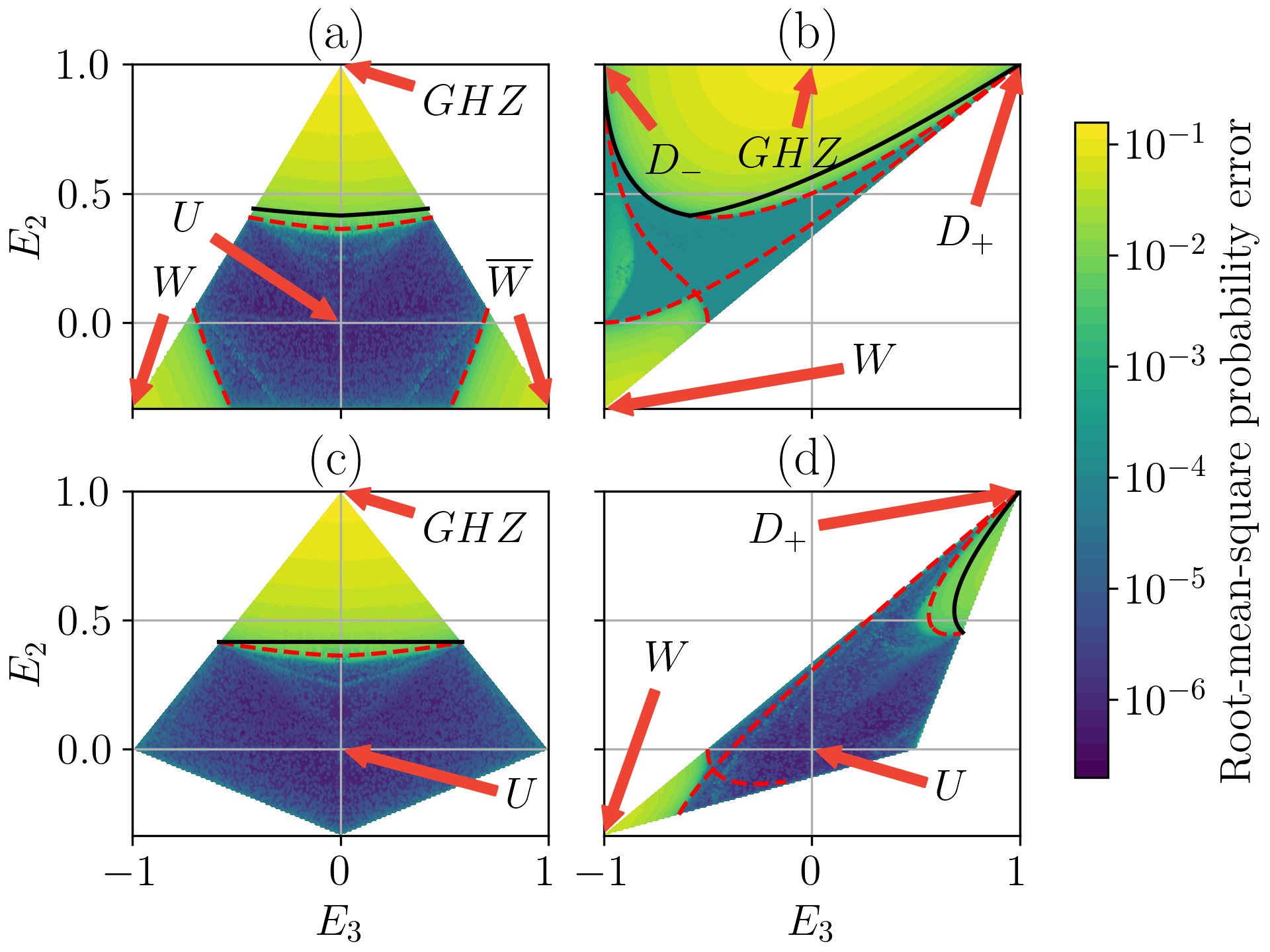
Figure 2: Euclidean distances between distributions of the form of Eq. (4) and best-fit triangle-local models (5) in the following affine subspaces: (a) mixtures of $U$, $GHZ$ and $W$; (b) mixtures of $D_{+}$, $D_{-}$ and $W$; (c) the plane $E_{1}=0$; (d) mixtures of $U$, $D_{+}$ and $W$. The dashed lines are generated by our proposed boundary models appropriate for each subspace. The solid line is the no-signaling independence (NSI) boundary given by inequality (15) of Ref. [27]. Regions with a potential for quantum non-locality are those between the dashed and solid lines.

An interesting observation is that, despite having performed the search with up to the sufficient cardinalities 666, for all the distributions that we find to admit triangle-local models the corresponding model has a smaller cardinality. In fact, we find that all local distributions of the form of Eq. (4) can be described by strategies where the latent variable cardinalities are 333, 322, 422, or 332. We give these models in Appendix B.

In Fig. 2 we show several sections of the tetrahedron of valid distributions that serve to illustrate our results. There, we plot the distance between the distribution and the best local model found. In all panels we observe sharp transitions, that we use to calculate the analytical boundaries later on (in dashed red).

Panel (a) shows distributions in the plane $3E_{1}+E_{3}=0$, which contains as vertices different forms of “full correlation”: the $GHZ$ distribution, corresponding to a shared random bit and characterized by $E_{1}=E_{3}=0$ and $E_{2}=1$, the $W$ distribution, corresponding to the uniform mixture of the parties outputting such that $a+b+c=1$ and characterized by $E_{1}=1/3$, $E_{2}=-1/3$ and $E_{3}=-1$, and the $\overline{W}$ distribution, corresponding to the uniform mixture of the parties outputting such that $a+b+c=-1$, characterized by $E_{1}=-1/3$, $E_{2}=-1/3$ and $E_{3}=1$. It also contains the uniformly random distribution, $U$, characterized by $E_{1}=E_{2}=E_{3}=0$. This panel clearly shows the three “islands of nonlocality” that appear in the scenario (see also Fig. 1b). It also illustrates the symmetry $E_{1},E_{2},E_{3}\rightarrow-E_{1},E_{2},-E_{3}$ that is present, corresponding to a bit-flip operation that switches the labels of all the outputs.

Panel (b) depicts the plane $E_{1}+E_{2}-E_{3}=1$, which is spanned by combinations of the $W$ distribution, and the two only deterministic distributions in the scenario: $D_{+}$, described by $E_{1}=E_{2}=E_{3}=1$, and $D_{-}$, described by $E_{1}=E_{3}=-1$ and $E_{2}=1$. In this plane we find an interesting transition: for $E_{3}<-2+\sqrt{2}$ we find triangle-local models that saturate the inequality given in Ref. [27] for distributions that admit a realization in the triangle scenario (depicted in black in the figure). However, for $E_{3}>-2+\sqrt{2}$, a gap between the inequality in Ref. [27] and the distributions with triangle-local models appears, signaling a region where quantum triangle nonlocality may be found.

Panel (c) illustrates the plane $E_{1}=0$, which was previously studied in Ref. [27] (see their Figure 3). We reproduce the results found there, finding an analytic expression for the boundary (see Bell inequalities below).

Finally, panel (d) contains the plane $E_{1}-2E_{2}+E_{3}=0$, which is spanned by the $W$ distribution, the $D_{+}$ distribution, and the uniform distribution $U$. Here, another gap between the inequality in Ref. [27] and the distributions with triangle-local models appears, signaling another region of interest for settling the conjecture in Ref. [29]. Interestingly, in the part of this figure close to the $W$ distribution, and also in the analogous region in panel (b), the boundary showcases a kink. This is caused by the fact that, as we will see below, the boundary in this area is given by the piecewise composition of a set of polynomial surfaces.

Bell inequalities.—

As can be seen in Figs. 1-3, there are only two boundaries that need to be characterized, namely that which is around the $GHZ$ distribution and that which is close to the $W$ distribution (the one close to $\overline{W}$ can be obtained from that close to $W$ via the transformation $E_{1},E_{2},E_{3}\rightarrow-E_{1},E_{2},-E_{3}$).

There is an important difference in the role of Bell inequalities (understood as the boundaries of the local set) in standard Bell scenarios and in networks, that stems from the convexity of the local set in the former and its non-convexity in the latter: While in Bell scenarios the violation of a single Bell inequality is sufficient to detect nonlocality, in general in networks a distribution needs to violate several Bell inequalities to be guaranteed to be nonlocal. This behavior is seen in other phenomena where the correlation sets are not convex, such as, e.g., full network nonlocality [34, 35]. Therefore, in the context of networks it is necessary to distinguish between Bell inequalities and tests of network nonlocality.

In the minimal triangle network, thus, there are only three tests that need to be performed to assess potential nonlocality: one for the $GHZ$-type nonlocality, one for the $W$-type nonlocality, and one for the $\overline{W}$-type nonlocality. In all cases, the distributions in the boundaries can be characterized with models that depend on two free parameters (see Appendix B). Inserting these models into the expressions for the correlators and using variable elimination techniques leads to expressions for the boundaries that are later used in the tests.

In Appendix C.1 we perform explicitly the variable elimination for the boundary around the $GHZ$ distribution (in blue in Figs. 1b, 3), giving that distributions of the form of Eq. (4) that admit a triangle-local model satisfy, at least, one of

$$8(1+E_{1})^{3}\left(11+37E_{1}+28E_{1}^{2}-4E_{1}^{3}+8E_{2}+13E_{1}E_{2}+E_{2}^{2}-11E_{3}-18E_{1}E_{3}-3E_{2}E_{3}+2E_{3}^{2}\right)-(3+5E_{1}+E_{2}-E_{3})^{4}\\ +\sqrt{(3+5E_{1}+E_{2}-E_{3})^{2}-8(1+E_{1})^{3}}\Big{[}\left(3+5E_{1}+E_{2}-E_{3}\right)^{3}-4\left(1+E_{1}\right)^{3}\left(7+11E_{1}+E_{2}-3E_{3}\right)\Big{]}\geq 0,$$ (6)

and its equivalent by performing $E_{1},E_{2},E_{3}\rightarrow-E_{1},E_{2},-E_{3}$. The strong numerical evidence that we build in this work leads us to conjecture that a criterion for detecting nonlocality in the binary-outcome triangle scenario is given by the simultaneous violation of Eq. (6) and its analogous via bit flips. Note that the square roots in Eq. (6) and its analogous under bit flips limits the distributions that can be tested with these witnesses, but if any of the expressions inside the square root is negative, the behavior does not exhibit $GHZ$-type nonlocality.

The boundaries close to $W$ and $\overline{W}$ are composed of five different regions (see Fig. 3). Performing analogous variable elimination processes, aided by software for symbolic computation using Gröbner bases [36], we give the remaining criteria for nonlocality, which consist of the simultaneous violations of five inequalities. We give such inequalities for the region close to the $W$ distribution in Appendix C.2. The ones corresponding to $\overline{W}$ can be obtained from them by the transformation $E_{1},E_{2},E_{3}\rightarrow-E_{1},E_{2},-E_{3}$.

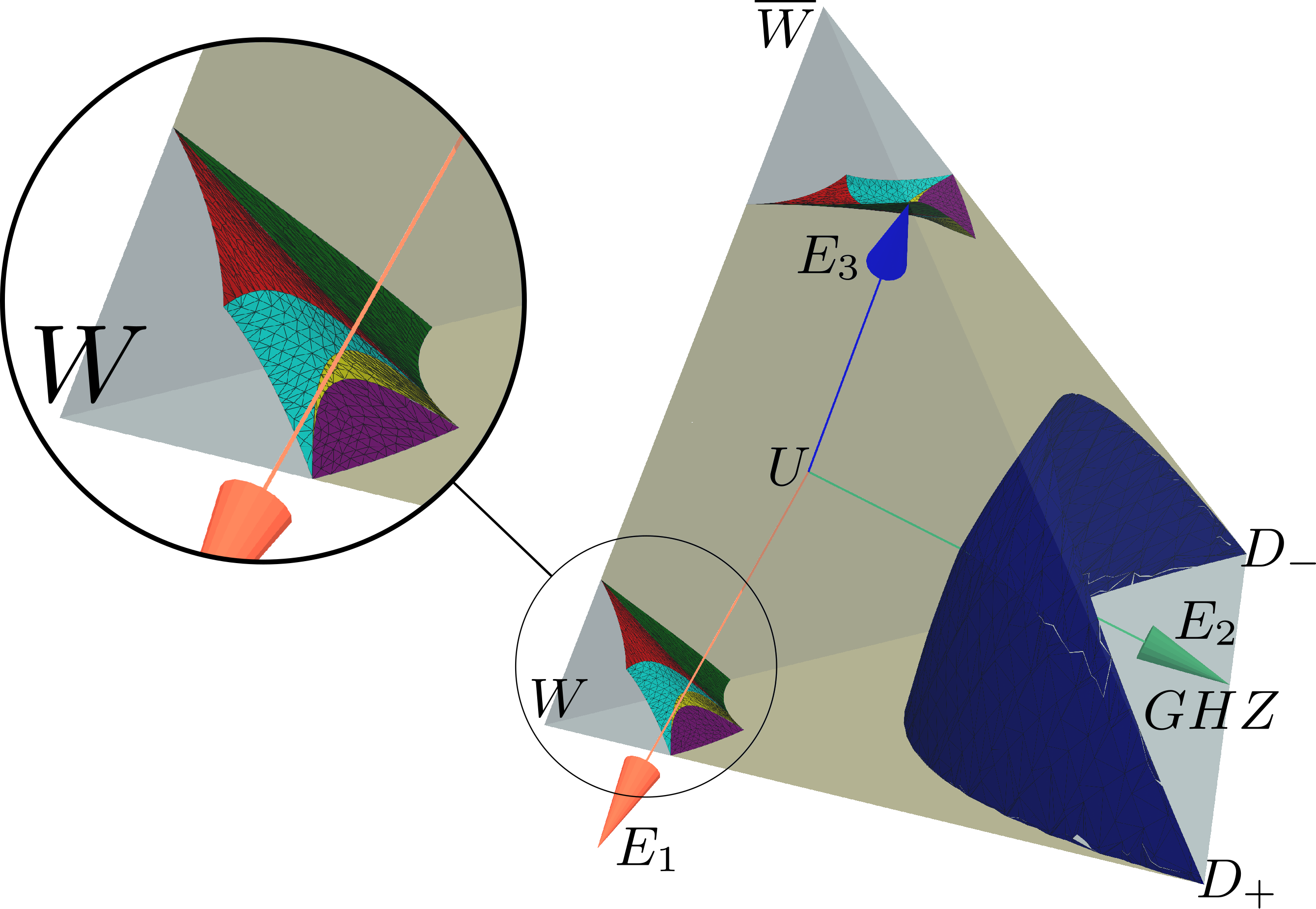
Figure 3: Zoomed-in, rotated version of Fig. 1b. The boundary close to the $GHZ$ distribution is shown in a single blue color, to indicate that it is given by only one inequality and its bit-flipped version. In contrast, the boundaries close to the $W$ and $\overline{W}$ distributions consist of the piecewise composition of five inequalities. The expressions for the families of network-local models that generate the inequalities and the inequalities themselves can be found in appendices B and C, respectively.

Perspectives for quantum nonlocality.—

The question of whether the binary-outcome triangle admits quantum distributions that cannot be reproduced by triangle-local models was posed in 2018 in Ref. [29] and, despite strong efforts (see, e.g., [27, 30, 28, 37, 38]), remains open. Our complete characterization of the set of symmetric distributions admitting triangle-local models allows us to provide new insights on this question. In particular, three regions previously not considered in the literature are, in panels (a), (b) and (d) of Fig. 2, those between the black lines (that represent the possible boundary of triangle-compatible distributions) and the red dashed lines that correspond to our inequalities.

Moreover, we can revisit regions that were previously studied. In particular, we focus on the regions that appear in Figures 2, 3 and Supplementary Figure 2 in Ref. [27]. There, the regions colored in yellow correspond to distributions that do not violate their necessary conditions to be compatible with the triangle scenario, but the reported search for triangle-local models fails. Figure 2 in Ref. [27] corresponds to the area with $E_{2}\leq\frac{1}{2}$ and $E_{3}\geq 0$ of panel (c) in Fig. 2. As mentioned before, we find the same boundary for distributions admitting triangle-local models as the one reported in Ref. [27], although we give an analytical expression for it, namely Eq. (6).

(a)

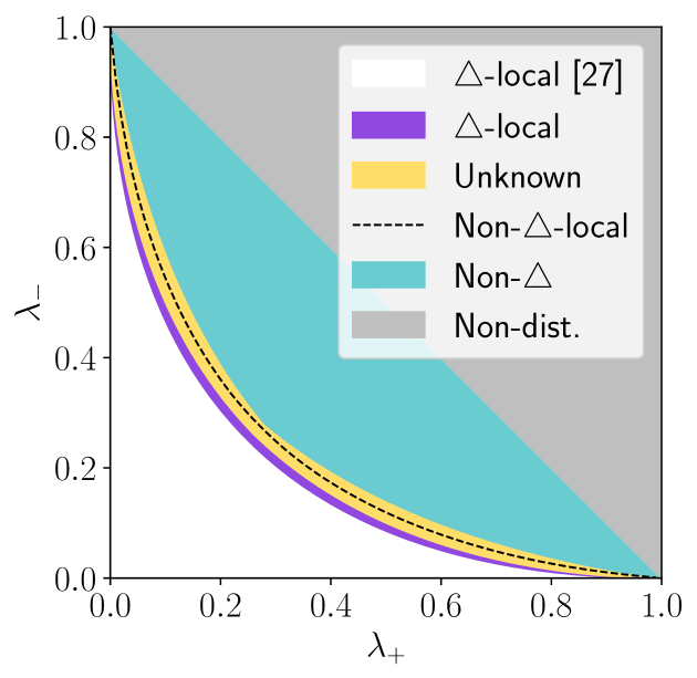
(b)

Figure 4: Reproductions of LABEL:sub@fig:e1e2 Figure 3 and LABEL:sub@fig:pq Supplementary Figure 2 in Ref. [27], with our improved characterizations. LABEL:sub@fig:e1e2 depicts the projection of the behavior space onto the $E_{1}$-$E_{2}$ plane, while LABEL:sub@fig:pq depicts the plane containing the distributions $D_{+}$, $D_{-}$, and $\left(W+\overline{W}\right)/2$. In both figures, the white regions contain the distributions that admit triangle-local models. The cyan regions contain the distributions that cannot be generated in the triangle network. The purple regions represent distributions for which we find triangle-local models, but were not identified in Ref. [27] to admit them. In LABEL:sub@fig:e1e2, the solid line represents the limit to the blue region given in Ref. [27]. In LABEL:sub@fig:pq, the dashed line represents our upper bound to the set of distributions admitting triangle-local models. Data for the white region in LABEL:sub@fig:e1e2 was provided by the authors of Ref. [27] on private communication.

For Figure 3 and Supplementary Figure 2 in Ref. [27], we extend the regions of distributions that admit triangle-local models, thereby reducing the regions where quantum nonlocality could appear. We reproduce such figures in Fig. 4, where the additional regions that we prove to have triangle-local models are depicted in purple. In Fig. 4a it is noteworthy to mention the distribution denoted by a black circle, which corresponds to $E_{1}=1/3$, $E_{2}=-5/27$ and $E_{3}=-5/9$. In the parameterization $\lambda_{W}W+\lambda_{+}D_{+}+\lambda_{-}D_{-}+(1-\lambda_{W}-\lambda_{+}-\lambda_{-})\overline{W}$, this distribution is the one with highest $\lambda_{W}$ that admits a triangle-local model. It admits a model with cardinalities $c_{\alpha}=c_{\beta}=c_{\gamma}=3$, described by the following distributions and response functions:

$$q(\alpha)=r(\beta)=s(\gamma)=\frac{1}{3}\quad\forall\,\alpha,\beta,\gamma\in\{1,2,3\},$$ (7)

$$A(-1|\beta,\gamma)=\delta_{\beta,1}\delta_{\gamma,1}+\delta_{\beta,1}\delta_{\gamma,3}+\delta_{\beta,2}\delta_{\gamma,3},$$

$$B(-1|\gamma,\alpha)=\delta_{\gamma,1}\delta_{\alpha,1}+\delta_{\gamma,2}\delta_{\alpha,1}+\delta_{\gamma,2}\delta_{\alpha,2},$$

$$C(-1|\alpha,\beta)=\delta_{\alpha,2}\delta_{\beta,3}+\delta_{\alpha,3}\delta_{\beta,2}+\delta_{\alpha,3}\delta_{\beta,3}.$$

In order to better analyze the potential for quantum nonlocality, we further constrain the set of distributions only subject to the conditions of no-signaling and independence of the sources in the network, using inflation methods [19]. The inflation corresponding to four copies of each of the sources (implemented with the inflation package in Python [39], see [33]) produces the cyan region in Fig. 4a, that improves over the boundary found in Ref. [27]. One can also use inflation methods to approximate the set of triangle-local distributions, at an increased computational cost. This limited the inflation we considered to that consisting of three copies of one source and two copies of the remaining ones, which produced worse bounds than those obtained by considering inflations tailored for arbitrary triangle-compatible distributions. In combination, our explicit triangle-local constructions and the improved outer approximations provided by inflation significantly reduce the set of distributions that could, in principle, demonstrate quantum non-locality. We expect that improved characterizations of the theory-agnostic distributions compatible with the triangle scenario in this region will reduce it further until closing the gap.

In Fig. 4b we also show that the region of distributions that admit triangle-local models is larger than that reported in Ref. [27]. Our boundary corresponds to the inequality (6), that we build from models where all the cardinalities are three. Here, inflation methods for triangle-compatible distributions did not produce improvements, suggesting that the inequality given in Ref. [27] may be tight in this region. However, using inflation tailored for triangle-local distributions we obtain an outer approximation (the black dashed line in Fig. 4b) that approaches closely our conjectured set. We expect that the remaining gap will be closed by improved outer characterizations. These results, despite reducing the region that could potentially host quantum nonlocality via the inner constructions, still signal it as a promising candidate where further effort should be put.

Discussion.—

In analogy with the study of Bell nonlocality, characterizing the probability distributions generated in networks that can be reproduced within classical physics is crucial for identifying genuinely quantum phenomena that can be exploited in applications such as quantum cryptography. In this work, using a combination of strong numerical analysis and analytical calculations, we give what we conjecture to be the complete characterization of the set of distributions symmetric under permutations of parties that admit a network-local model in the binary-outcome triangle scenario.

The analysis, based on, both, explicit constructions of network-local models and outer approximations of the whole set, was performed using readily available tools [40, 39] that can be easily adapted to more complex networks and input-output scenarios. These tools, or improved ones, will have a prominent role in the analysis of quantum networks. However, the fact that the amount of resources scales unfavourably with the complexity of the scenario motivates the search for more efficient characterization methods.

We show that symmetric, binary-outcome, triangle-local distributions can be characterized without saturating the cardinality bounds of Ref. [31]. Finding a physical explanation of why this is the case, and whether the bound is saturated in the case of non-symmetric distributions, are interesting questions that we leave open.

Our improved characterization rules out some regions of the parameter space thought to be promising for demonstrating quantum nonlocality. Other regions (including new ones that we identify), however, persist as valid candidates to support genuinely quantum behaviors. Still, more work is needed to decide the conjecture of Ref. [29], which crucially will require improved methods for explicitly constructing quantum realizations in networks.

Appendix A Details on the numerical search

In this appendix we provide all the details of the determination of the set of triangle-local distributions and of its boundaries. The workflow is summarized in Fig. 5. Each step is described below in detail.

Figure 5: Flowchart of the search for triangle-local models in this work. Numerical steps are highlighted in blue, and analytical steps are highlighted in green.

Our process begins with the selection of some 2-dimensional affine subspaces in the behavior space, whose distributions are subjected to an exploratory search of local models. The subspaces that were investigated in the first round of the analysis were the affine combinations of i) $U$, $GHZ$, and $W$, ii) $D_{+}$, $D_{-}$, and $W$, iii) $U$, $D_{+}$, and $W$, iv) $U$, $D_{+}$, and $GHZ$, as well as v) the plane $E_{1}=0$. All of them contain both local distributions (such as $U$, $D_{+}$, $D_{-}$) and nonlocal ones (such as $GHZ$, $W$, $\overline{W}$), so they all feature local-nonlocal transitions, as can be seen in Fig. 2 of the main text. Moreover, the plane $E_{1}=0$ has been previously analyzed in Ref. [27].

In each plane, we sample approximately 10.000 distributions by uniformly sampling $E_{1}$, $E_{2}$, and $E_{3}$ subject to the corresponding constraints. For each of these, we try to fit a local model to the target distribution, by minimizing the sum of squared errors on the probabilities. We implement and solve this problem using the scipy library in Python (see the computational appendix [33]). Initially, we set the hidden variable cardinalities to $c_{\alpha}=c_{\beta}=c_{\gamma}=6$, which is guaranteed to generate the complete triangle-local set [31]. For subsequent rounds, the computations were expedited by lowering the cardinalities to $c_{\alpha}=c_{\beta}=c_{\gamma}=4$, or even $c_{\alpha}=c_{\beta}=c_{\gamma}=3$ in some subspaces, since these reduced cardinalities were enough to generate points on the local boundary. For each distribution, we run the optimization 200 times, each one with a different, uniformly random initial guess for $q$, $r$, $s$, $A$, $B$, and $C$, and take the model with the lowest error to the target behavior.

After the search for models, we look at those with root-mean-square probability error of the order of $10^{-4}$, since these are close to the sharp transitions of the error heat maps, such as the ones depicted in Fig. 2 of the main text. These models typically have several parameters that take on values close to $0$ or $1$. The model inference procedure then consists of fixing these parameters to be exactly equal to the extreme values, and solving for the remaining parameters by enforcing the symmetry constraints. Unlike the exploratory analysis, this is done analytically (see a more detailed discussion in appendices C and D).

The output of the model inference step are models which turn out to have two free parameters, thus they span surfaces in $(E_{1},E_{2},E_{3})$ space. These surfaces are joined to form the tentative boundaries of the local set, which perform well in capturing the local-nonlocal transitions in the 2-dimensional error plots. Naturally, this is expected, since the boundary models are derived from the optimization results in the very same regions, so a more meaningful test for these surfaces should consider the whole behavior space, going beyond the affine subspaces of the exploratory analysis. That is the purpose of the boundary validation procedure, following the flowchart of Fig. 5.

For this test, we sample 1.000 distributions on each of the proposed boundaries, and slightly displace them by an euclidean distance of $10^{-3}$ (in correlator space) towards the archetypal nonlocal distributions, $GHZ$ or $W$ depending on the boundary being tested, so that we have distributions just outside the provisional local set. These 2.000 distributions (the original 1.000, and the corresponding displaced ones) are then subjected to a local model search with 1.000 trials per distribution. The optimization runs of this boundary validation procedure are always performed with the full cardinalities $c_{\alpha}=c_{\beta}=c_{\gamma}=6$.

Out of these 2.000 optimized models, the ones that achieve probability error of the order of $10^{-4}$ or lower are further analyzed. Most of them are equivalent to the boundary models, when considering hidden variable exchanges and relabellings. The genuinely new ones generate points that, despite being beyond the proposed local boundary, admit a triangle-local model. These are the violations mentioned in Fig. 5, that indicate that the local boundary should be improved with more powerful models. While the boundary close to $GHZ$ distribution had no violations in the validation test already in the first run, the boundary close to the $W$ distribution needed three cycles of gradual improvement in order to finally pass this check.

If the general structure of the improved models can be inferred from the boundary violations, the new cycle begins with the model inference step. Otherwise, we add more subspaces to the exploratory analysis phase, as shown in Fig. 5. These additional subspaces are chosen in a way to be close to the violations found in the previous step, so as to capture the features that were missing in the previous set of subspaces. At the end of the process, we had to add the following planes to our initial collection: vi) $3E_{1}+3E_{2}-E_{3}=1$, vii) $E_{1}+(4+2\sqrt{5})E_{2}+E_{3}=0$, viii) $12E_{1}-4E_{2}+6E_{3}=1$, as well as ix) the affine combinations of $D_{+}$, $W$, and $\overline{W}$.

Appendix B Models for distributions at the boundaries

In this appendix we give the concrete families of triangle-local models (5) that describe the distributions invariant under permutations of parties that lie in the boundaries of the network-local set for the binary-outcome triangle network. For ease in the notation, we represent $q$, $r$ and $s$ by one-dimensional arrays that contain the corresponding probabilities, and $A\equiv A(1|\beta,\gamma$), $B\equiv B(1|\gamma,\alpha)$ and $C\equiv C(1|\alpha,\beta)$ by two-dimensional arrays. In each of these, the first hidden variable indexes the rows, while the second one indexes the columns. The arrays corresponding to the outcomes $-1$ can be obtained by using the normalization condition.

B.1 Models for the boundary close to the GHZ distribution

The boundary close to the $GHZ$ distribution (in blue in Figs. 1b and 3) is described by a single family of models. It has cardinalities $c_{\alpha}=c_{\beta}=c_{\gamma}=3$ and is given by

$$q(\omega)=r(\omega)=s(\omega)=\begin{cases}x&\omega=1\\ y&\omega=2\\ 1-x-y&\omega=3\end{cases},\qquad\begin{matrix}A(1|\omega,\mu)\\ B(1|\omega,\mu)\\ C(1|\omega,\mu)\end{matrix}=\begin{cases}1&(\omega,\mu)\in\{(1,2),(2,1),(2,2)\}\\ 0&\text{otherwise}\end{cases}$$ (8)

for arbitrary, positive $x$ and $y$ satisfying $x+y\leq 1$. In the notation that was described above, this model takes the form

$$q=r=s=\begin{bmatrix}x&y&1-x-y\end{bmatrix},\,A=B=C=\begin{bmatrix}0&1&0\\ 1&1&0\\ 0&0&0\end{bmatrix}.$$ (9)

This model characterizes only half of the boundary. The other half is described by the model with the outcomes flipped, which amounts to doing $A\rightarrow 1-A$, $B\rightarrow 1-B$ and $C\rightarrow 1-C$ in Eq. (9). Note that the family is described by two free parameters, $x$ and $y$.

B.2 Models for the boundary close to the W distribution

The situation is considerably richer for the boundary close to the $W$ distribution, where there are five different classes of models that generate different sections of the surface, as depicted in Fig. 3 in the main text. The models that characterize the boundary close to the $\overline{W}$ distribution are the same as those presented below when replacing $A\rightarrow 1-A$, $B\rightarrow 1-B$ and $C\rightarrow 1-C$.

B.2.1 Model for the green surface

The distributions on the green surface admit the following model with cardinalities $c_{\alpha}=3$, $c_{\beta}=c_{\gamma}=2$:

$$q=\begin{bmatrix}1-2x&x&x\end{bmatrix},\,r=s=\begin{bmatrix}y&1-y\end{bmatrix},\,A=\begin{bmatrix}z(x,y)&1\\ 1&t(x,y)\end{bmatrix},\,B=\begin{bmatrix}1&0&1\\ 0&0&1\end{bmatrix},\,C=\begin{bmatrix}1&0\\ 1&1\\ 0&0\end{bmatrix},$$ (10)

where $z(x,y)=\dfrac{2x^{2}y-x^{2}-4xy^{2}+xy+2y^{2}-y}{y^{2}(1-2x)}$ and $t(x,y)=\dfrac{x(1-x-y+2xy)}{1-2x-2y+4xy+y^{2}-2xy^{2}}$. The free parameters of the family are $x$ and $y$, which satisfy $0\leq x\leq x_{\mathrm{max}}$ and $1+x+\sqrt{\dfrac{1+5x^{2}-2x^{3}}{1-2x}}\leq 4y\leq 4-2x\left(1+\sqrt{\dfrac{5-2x}{1-2x}}\right),$ $x_{\mathrm{max}}$ being the smallest real root of the polynomial $9x^{4}-24x^{3}+24x^{2}-9x+1$, namely

$$x_{\mathrm{max}}= \,\frac{2}{3}-\frac{1}{6\sqrt{\frac{3}{\sqrt[3]{\frac{675}{2}-\frac{81\sqrt{41}}{2}}+3\sqrt[3]{\frac{1}{2}\left(3\sqrt{41}+25\right)}}}}$$

$$-\frac{1}{2}\sqrt{-\frac{1}{27}\sqrt[3]{\frac{675}{2}-\frac{81\sqrt{41}}{2}}-\frac{1}{9}\sqrt[3]{\frac{1}{2}\left(3\sqrt{41}+25\right)}+\frac{10}{3\sqrt{3\left(\sqrt[3]{\frac{675}{2}-\frac{81\sqrt{41}}{2}}+3\sqrt[3]{\frac{1}{2}\left(3\sqrt{41}+25\right)}\right)}}}$$

$$\approx \,0.1916.$$

B.2.2 Model for the purple surface

The distributions on the purple surface admit the following model with cardinalities $c_{\alpha}=4$, $c_{\beta}=c_{\gamma}=2$:

$$q=\begin{bmatrix}z(x,y)&z(x,y)&t(x,y)&1-2z(x,y)-t(x,y)\end{bmatrix},\,r=s=\begin{bmatrix}x&1-x\end{bmatrix},\,A=\begin{bmatrix}0&1\\ 1&1\end{bmatrix},\,B=\begin{bmatrix}y&1&1&0\\ 0&1&0&1\end{bmatrix},\,C=\begin{bmatrix}1&1\\ y&0\\ 1&0\\ 0&1\end{bmatrix},$$ (11)

where $z(x,y)=\dfrac{(x-1)^{3}x}{1-4x+6x^{2}-4x^{3}-xy+x^{2}y+x^{3}y}$, $t(x,y)=\dfrac{(x-1)x^{3}(1-y)}{1-4x+6x^{2}-4x^{3}-xy+x^{2}y+x^{3}y}$. Again, $x$ and $y$ are the free parameters of the family of models. In this case, they satisfy $0\leq y\leq 1$ and $x_{\mathrm{min}}\leq x\leq 1$, $x_{\mathrm{min}}$ being the only positive root of the polynomial $(3-y)x^{4}-3x^{3}-yx^{2}+(2+y)x-1$ for $y\not=1$ and $x_{\mathrm{min}}(y=1)=\frac{1}{2}$.

B.2.3 Model for the red surface

The distributions on the red surface admit the following model with cardinalities $c_{\alpha}=c_{\beta}=c_{\gamma}=3$:

$$q=r=\begin{bmatrix}x&z(x,y)&1-x-z(x,y)\end{bmatrix},\,s=\begin{bmatrix}y&\dfrac{1-y}{2}&\dfrac{1-y}{2}\end{bmatrix},$$

$$A=\begin{bmatrix}0&1&0\\ 1&1&0\\ 1&1&1\end{bmatrix},\,B=\begin{bmatrix}0&1&1\\ 0&0&1\\ 1&1&1\end{bmatrix},\,C=\begin{bmatrix}t(x,y)&1&1\\ 1&u(x,y)&0\\ 1&0&0\end{bmatrix},$$ (12)

where the functions $z$, $t$, and $u$ are $z(x,y)=\dfrac{x-x^{2}-2y+4xy-x^{2}y+xy^{2}}{(x-y)(1-y)}$, $t(x,y)=\dfrac{x-4(1-x)^{3}y+(3-4x)xy^{2}}{4x^{2}y(x-y)}$, and $u(x,y)=\dfrac{(x-y)(1-y)^{2}[4y(1+x^{2}+x^{3}-x^{2}y)-x-xy(10+y)]}{4y(x-x^{2}-2y+4xy-x^{2}y+xy^{2})^{2}}$. As before, the probabilities $x$ and $y$ are the free parameters of the family, which satisfy $1/3\leq y\leq 1$ and $\frac{1}{24y}\mathrm{max}\Big{[}1+12y+3y^{2}-\sqrt{\left(1+12y+3y^{2}\right)^{2}-192y^{2}},$ $12y\left(2+y-\sqrt{2+2y+y^{2}}\right)\Big{]}\leq x\leq x_{\mathrm{max}}$, $x_{\mathrm{max}}$ being the smallest root of the polynomial $16y^{2}x^{4}-12y(1+2y+5y^{2})x^{3}+(1+12y+34y^{2}+84y^{3}+45y^{4})x^{2}-(5+16y+50y^{2}+24y^{3}+y^{4})yx+4y^{2}(1+y)^{2}$.

Model (7) of the main text produces a behavior on the intersection of the red and cyan surfaces in Fig. 3, so it can be regarded as a member of the family (12), with $x=\frac{1}{3}+\varepsilon$, $y=\frac{1}{3}+4\varepsilon$ and then taking the limit $\varepsilon\rightarrow 0$.

B.2.4 Model for the yellow surface

The distributions on the yellow surface admit the following model with cardinalities $c_{\alpha}=c_{\beta}=3$, $c_{\gamma}=2$:

$$q=\begin{bmatrix}z(x,y)&t(x,y)&1-z(x,y)-t(x,y)\end{bmatrix},$$

$$r=\begin{bmatrix}u(x,y)&v(x,y)&1-u(x,y)-v(x,y)\end{bmatrix},$$

$$s=\begin{bmatrix}x&1-x\end{bmatrix},$$

$$A=\begin{bmatrix}0&1\\ 1&1\\ 0&0\end{bmatrix},\,B=\begin{bmatrix}y&1&1\\ 1&1&0\end{bmatrix},\,C=\begin{bmatrix}0&0&1\\ 1&0&1\\ 1&1&1\end{bmatrix}.$$ (13)

In the model above, $z(x,y)$ is the largest root of the polynomial

$$(1 -y)^{2}(1-x+x^{2}y)(1-x+xy+xy^{2})z^{2}$$ (14)

$$-(1-y)(x-2x^{2}+x^{3}-2y+5xy-3x^{2}y+x^{3}y-x^{4}y-x^{2}y^{2}+x^{3}y^{2}+x^{4}y^{2}+x^{2}y^{3}-x^{3}y^{3})z$$

$$-(1-x)(x-y)y(1-x+xy).$$

Based on it, and on the free parameters $x$ and $y$ (constrained only by the requirements of all probabilities being positive), the remaining parameters are

$$t(x,y) =\dfrac{1-2z-x+2xz-xy^{2}z}{1-x+y},$$

$$u(x,y) =\dfrac{(1-y)(1-z-x+xz+yz+xy-xyz-x^{2}yz+x^{2}y^{2}z)}{(1-x+y)(1-x+xy)},$$

$$v(x,y) =\frac{y}{1-y}\,u(x,y).$$

B.2.5 Model for the cyan surface

Finally, distributions on the cyan surface admit the following model with cardinalities $c_{\alpha}=c_{\beta}=c_{\gamma}=3$:

$$q=\begin{bmatrix}x&y&1-x-y\end{bmatrix},\,r=\begin{bmatrix}z&t&1-z-t\end{bmatrix},\,s=\begin{bmatrix}u&v&1-u-v\end{bmatrix},\,A=\begin{bmatrix}0&1&0\\ 1&1&0\\ 1&1&1\end{bmatrix},\,B=\begin{bmatrix}0&1&1\\ 0&0&1\\ 1&1&1\end{bmatrix},\,C=\begin{bmatrix}w&1&1\\ 1&1&0\\ 1&0&0\end{bmatrix},$$ (15)

where the seven probabilities $x$, $y$, $z$, $t$, $u$, $v$, and $w$ can be parameterized as complicated functions of the correlators $E_{1}$ and $E_{2}$, that serve as the two free parameters for the model. The complete characterization of this model is provided in appendix D.

As mentioned before, model (7) of the main text is also a member of the family (15). By fixing $E_{1}=1/3$ and $E_{2}=-5/27$, and following the procedure of appendix D, the parameters $x$ and $z$ are obtained exactly by solving a system of polynomial equations that has 44 solutions, one of them being $x=z=1/3$. The other parameters readily follow from the symmetry and correlator constraints. Alternatively, the same result can be obtained numerically with the routine that generate points on the cyan surface, provided in [33].

Appendix C List of tests for triangle nonlocality

In this appendix we give, both, the Bell inequalities that characterize the boundaries of the set of distributions that admit triangle-local models, and the associated tests of nonlocality. As explained in the main text, the direct connection between Bell inequalities and tests for nonlocality that is drawn in Bell-type scenarios cannot be made in networks due to the fact that the sets of network-local correlations are not convex. A distribution can be considered as network-nonlocal only if it violates, in general, several Bell-like inequalities. Thus, we distinguish between Bell inequalities (i.e., the boundaries of the set of distributions that admit network-local models), and tests for network nonlocality.

Each of the subsections below describes a different test of network nonlocality. Passing any of them identifies a distribution as network-nonlocal. However, each of the tests involves the violation of several inequalities, and all the inequalities in a test must be violated in order to pass the test. The inequalities that determine the boundary of the set of symmetric, network-local distributions are Eqs. (19), (20), (21), (22), (23), and (24), as well as their counterparts under the transformation $E_{1},E_{2},E_{3}\rightarrow-E_{1},E_{2},-E_{3}$.

The computational appendix [33] for this work contains Python implementations of all the tests and inequalities described below, routines to generate points on the local boundaries, and a script to render an interactive version of Fig. 1b of the main text.

C.1 Test for network nonlocality close to the GHZ distribution

The family of models that describe the boundary close to the $GHZ$ distribution has cardinalities $c_{\alpha}=c_{\beta}=c_{\gamma}=3$ and is given by

$$q(\omega)=r(\omega)=s(\omega)=\begin{cases}x&\omega=1\\ y&\omega=2\\ 1-x-y&\omega=3\end{cases},$$ (16)

$$\begin{matrix}A(1|\omega,\mu)\\ B(1|\omega,\mu)\\ C(1|\omega,\mu)\end{matrix}=\begin{cases}1&(\omega,\mu)\in\{(1,2),(2,1),(2,2)\}\\ 0&\text{otherwise}\end{cases}$$

for arbitrary, positive $x$ and $y$ satisfying $x+y\leq 1$. When Eq. (16) is inserted into Eq. (5), and then into Eq. (4), the correlators become

$$E_{1} =-1+4xy+2y^{2},$$ (17a)

$$E_{2} =1-8xy+4x^{2}y-4y^{2}+12xy^{2}+4y^{3},$$ (17b)

$$E_{3} =-1+12xy-12x^{2}y+6y^{2}-12xy^{2}-4y^{3}.$$ (17c)

Equation (17a) can easily be solved for $x$, giving $x=(1+E_{1}-2y^{2})/(4y)$. Substituting this into Eqs. (17b) and (17c), we get depressed quartic equations in $y$, namely

$$E_{2} =\frac{(1+E_{1})^{2}}{4y}-1-2E_{1}+2y(1+E_{1})-y^{3},$$ (18a)

$$E_{3} =-\frac{3(1+E_{1})^{2}}{4y}+2+3E_{1}-y^{3}.$$ (18b)

Subtracting Eq. (18b) from Eq. (18a) yields a simpler quadratic equation. Solving it provides an expression for $y$ in terms of the correlators, ultimately resulting in a single equation that leads to the inequality

$$8(1+E_{1})^{3}\left(11+37E_{1}+28E_{1}^{2}-4E_{1}^{3}+8E_{2}+13E_{1}E_{2}+E_{2}^{2}-11E_{3}-18E_{1}E_{3}-3E_{2}E_{3}+2E_{3}^{2}\right)-(3+5E_{1}+E_{2}-E_{3})^{4}\\ +\sqrt{(3+5E_{1}+E_{2}-E_{3})^{2}-8(1+E_{1})^{3}}\Big{[}\left(3+5E_{1}+E_{2}-E_{3}\right)^{3}-4\left(1+E_{1}\right)^{3}\left(7+11E_{1}+E_{2}-3E_{3}\right)\Big{]}\geq 0.$$ (19)

Proceeding analogously with the bit-flipped version of the model (16) (which amounts to performing the transformation $E_{1}\rightarrow-E_{1}$, $E_{2}\rightarrow E_{2}$, $E_{3}\rightarrow-E_{3}$), we obtain the second inequality that characterizes the boundary of the network-local close to the $GHZ$ distribution.

The associated test of nonlocality consists on the simultaneous violation of, both, Eq. (19) and its bit-flipped version. In other words, a distribution is guaranteed not to admit a triangle-local model if it violates, both, Eq. (19) and its bit-flipped version.

Note that the inequalities contain square roots which could, in principle, take negative values for some distributions. For instance, the argument of the square root in Eq. (19) evaluates to $-\frac{64}{27}$ in the $\overline{W}$ distribution. This sets a limit on the distributions that can be detected with this test to only those for which (naturally) the left-hand sides evaluate to negative real numbers. When any of the left-hand sides is positive or complex, either the corresponding distribution admits a triangle-local model or it violates one of the remaining tests, that we give in the next section.

C.2 Tests for network nonlocality close to the $W$ and $\overline{W}$ distributions

Now we address the regions close to the $W$ and $\overline{W}$ distributions. In fact, we just need to study one of them, since the other is obtained from it by performing the transformation $E_{1},E_{2},E_{3}\rightarrow-E_{1},E_{2},-E_{3}$.

Let us, without loss of generality, focus on the boundary close to the $W$ distribution. This boundary is a continuous (but not everywhere smooth) piecewise composition of five surfaces. Nonlocal distributions in this region violate all the inequalities (20)-(24). In order to obtain them, we have performed the same parameter elimination process described in the previous section to the five families of models that describe the boundary of the set close to the $W$ distribution (i.e., those given by Eqs. (10)-(15)). For some of them, this can be done in a straightforward manner by using two correlator equations to solve for the degrees of freedom, and then substituting these expressions in the remaining correlator. For the remaining ones, the equations result in high-degree polynomials with no explicit solutions involving elementary operations. In such cases, we used software for symbolic computation to perform the elimination with the aid of Gröbner bases [36].

The simplest inequality found is that associated with model (10), given by

$$-E_{1}E_{2}+E_{3}+(1-E_{1})\sqrt{(1+E_{2})^{2}-4E_{1}^{2}}\geq 0.$$ (20)

In contrast with Eq. (19), in this case the expression inside the square root in inequality is always nonnegative due to the positivity constraints.

The next inequality is the one associated with model (11). It is a polynomial inequality of degree 5, but notice that it is only relevant if an auxiliary condition on $E_{1}$ is satisfied:

$$8E_{1}^{5}-15E_{1}^{4}-16E_{1}^{3}E_{2}+22E_{1}^{3}+16E_{1}^{2}E_{2}^{2}-2E_{1}^{2}E_{2}-20E_{1}^{2}-6E_{1}E_{2}^{2}+12E_{1}E_{2}+10E_{1}-E_{2}^{2}-6E_{2}$$

$$\quad+E_{3}^{2}\left(E_{1}^{2}-2E_{1}+2\right)+E_{3}\left(6E_{1}^{3}-8E_{1}^{2}E_{2}-12E_{1}^{2}+10E_{1}E_{2}+10E_{1}-8E_{2}\right)-1\geq 0,$$ (21)

$$\text{{provided} }E_{1}\geq 1/3.$$

If the auxiliary condition $E_{1}\geq 1/3$ is false, inequality (21) need not be evaluated and should be considered violated. These auxiliary conditions are occasionally necessary because each of the surfaces defining the $W$ boundary has a different range of validity when projected onto the $E_{1}$-$E_{2}$ plane.

Related to model (12), we obtain the following inequality of degree 5, with two auxiliary conditions on $E_{1}$ and $E_{2}$:

$$2(1+E_{1})E_{3}^{3}+27(1-3E_{1}+4E_{1}^{2}+E_{2}-2E_{1}E_{2})(1-E_{1}+2E_{1}^{3}+2E_{2}-E_{1}E_{2}+E_{2}^{2})$$

$$\quad+54E_{1}E_{3}(2-5E_{1}+5E_{1}^{2}+3E_{2}-4E_{1}E_{2}+E_{2}^{2})-9E_{3}^{2}(1-2E_{1}-6E_{1}^{2}+E_{2}+2E_{1}E_{2})\geq 0,$$ (22)

$$\begin{aligned} &\text{{provided} }&&-2048E_{1}^{12}+8E_{1}^{11}(479+128E_{2})-36E_{1}^{10}(153+61E_{2})-6E_{1}^{9}(2033+466E_{2}+177E_{2}^{2})\\ &&&\quad+3E_{1}^{8}(6687+7809E_{2}+181E_{2}^{2}+243E_{2}^{3})-4E_{1}^{7}(2021+7383E_{2}+3159E_{2}^{2}-351E_{2}^{3})\\ &&&\quad+8E_{1}^{6}(177+3460E_{2}+264E_{2}^{2}-171E_{2}^{3})-4E_{1}^{5}(2303+581E_{2}+10892E_{2}^{2}-39E_{2}^{3}-621E_{2}^{4})\\ &&&\quad+2E_{1}^{4}(8625+12715E_{2}-9853E_{2}^{2}+9081E_{2}^{3}+1728E_{2}^{4})\\ &&&\quad-4E_{1}^{3}(2335+11013E_{2}+8469E_{2}^{2}-4405E_{2}^{3}-666E_{2}^{4})\\ &&&\quad+4E_{1}^{2}(125+3175E_{2}+7926E_{2}^{2}+5032E_{2}^{3}-212E_{2}^{4}-108E_{2}^{5})\\ &&&\quad+E_{1}(506+624E_{2}-2682E_{2}^{2}-5100E_{2}^{3}-2268E_{2}^{4})-71-369E_{2}-477E_{2}^{2}-243E_{2}^{3}\geq 0,\\ &\text{ {and} }&&4E_{1}^{2}(3-2E_{1}+E_{2}+E_{1}^{2})-(1-2E_{1})(1+E_{2})^{2}\geq 0,\\ &\text{ {and} }&&E_{3}\geq 6-3\sqrt{5}.\end{aligned}$$

If any of the three auxiliary conditions is false, then inequality (22) should be considered violated.

Next, model (13) leads to a polynomial inequality of degree 8:

$$-(1-E_{3})^{5}(1+E_{1})+(1-E_{3})^{4}(2+E_{1}+9E_{1}^{2}-2E_{1}^{3}-3E_{2}-7E_{1}E_{2})+2(1-E_{3})^{3}(E_{1}-E_{2})(3E_{1}-17E_{1}^{2}+4E_{1}^{3}+E_{2}+9E_{1}E_{2})\\ -2(1-E_{3})^{2}\Big{(}30E_{1}^{2}-65E_{1}^{3}+43E_{1}^{4}-18E_{1}^{5}-8E_{2}+4E_{1}E_{2}+E_{1}^{2}E_{2}+21E_{1}^{3}E_{2}+12E_{1}^{4}E_{2}-2E_{2}^{2}+17E_{1}E_{2}^{2}\\ -43E_{1}^{2}E_{2}^{2}-2E_{1}^{3}E_{2}^{2}-E_{2}^{3}+11E_{1}E_{2}^{3}\Big{)}-(1-E_{3})\Big{(}16E_{1}^{2}-128E_{1}^{3}+261E_{1}^{4}-227E_{1}^{5}+88E_{1}^{6}-16E_{2}\\ +80E_{1}E_{2}-300E_{1}^{3}E_{2}+428E_{1}^{4}E_{2}-232E_{1}^{5}E_{2}-48E_{2}^{2}+128E_{1}E_{2}^{2}-58E_{1}^{2}E_{2}^{2}-130E_{1}^{3}E_{2}^{2}+168E_{1}^{4}E_{2}^{2}-32E_{2}^{3}\\ +68E_{1}E_{2}^{3}-36E_{1}^{2}E_{2}^{3}-40E_{1}^{3}E_{2}^{3}-3E_{2}^{4}+13E_{1}E_{2}^{4}\Big{)}+48E_{1}^{3}-6E_{1}^{4}-515E_{1}^{5}+1101E_{1}^{6}-882E_{1}^{7}+256E_{1}^{8}\\ -48E_{1}E_{2}+48E_{1}^{2}E_{2}+280E_{1}^{3}E_{2}-467E_{1}^{4}E_{2}-71E_{1}^{5}E_{2}+504E_{1}^{6}E_{2}-256E_{1}^{7}E_{2}+48E_{2}^{2}-224E_{1}E_{2}^{2}\\ +220E_{1}^{2}E_{2}^{2}+298E_{1}^{3}E_{2}^{2}-598E_{1}^{4}E_{2}^{2}+212E_{1}^{5}E_{2}^{2}+64E_{1}^{6}E_{2}^{2}+64E_{2}^{3}-200E_{1}E_{2}^{3}+82E_{1}^{2}E_{2}^{3}\\ +218E_{1}^{3}E_{2}^{3}-184E_{1}^{4}E_{2}^{3}+26E_{2}^{4}-39E_{1}E_{2}^{4}-7E_{1}^{2}E_{2}^{4}+30E_{1}^{3}E_{2}^{4}+E_{2}^{5}-3E_{1}E_{2}^{5}\geq 0.$$ (23)

Finally, we give the inequality related to model (15) expressed as

$$E_{3}\geq f(E_{1},E_{2}),$$ (24)

where $f$ is a complicated function, described in Appendix D.

It is important to recall that the test for network nonlocality entails checking the violation of all Eqs. (20)-(24). If a distribution does not violate all of them, then it is not in the nonlocal region close to the $W$ distribution, and might even be local, if it does not pass the remaining tests.

Appendix D Characterization of model (15) and inequality (24)

With the exception of model (11), all the other models that characterize distributions in the boundary close to the $W$ distribution are particular cases of the following general 333 model, up to hidden variable exchanges and relabellings:

$$q=\begin{bmatrix}x&y&1-x-y\end{bmatrix},\,r=\begin{bmatrix}z&t&1-z-t\end{bmatrix},\,s=\begin{bmatrix}u&v&1-u-v\end{bmatrix},\,A=\begin{bmatrix}0&1&0\\ 1&1&0\\ 1&1&1\end{bmatrix},\,B=\begin{bmatrix}0&1&1\\ 0&0&1\\ 1&1&1\end{bmatrix},\,C=\begin{bmatrix}w&1&1\\ 1&k&0\\ 1&0&0\end{bmatrix},$$ (25)

subject to the positivity constraints

$$x\geq 0,\,\,y\geq 0,\,\,x+y\leq 1,\,\,z\geq 0,\,\,t\geq 0,\,\,z+t\leq 1,\,\,u\geq 0,\,\,v\geq 0,\,\,u+v\leq 1,\,\,0\leq w\leq 1,\,\,0\leq k\leq 1.$$ (26)

This model has four degrees of freedom (eight parameters minus four symmetry constraints), and it spans a volume in $(E_{1},E_{2},E_{3})$ space. In order to find the boundary of this volume closest to the $W$ distribution, it suffices to solve the constrained optimization problem of finding the combination of parameters that minimizes $E_{3}$ for fixed values of $E_{1}$ and $E_{2}$, while satisfying the positivity and symmetry constraints. By numerically solving this problem, we found which positivity constraints saturate depending on the values of $E_{1}$ and $E_{2}$. This way, the general model (25) splits into four different subclasses. For each subclass, the problem of minimizing $E_{3}$ is much more manageable and can be tackled analytically, yielding the models presented in Appendix B:

Saturated positivity constraints (26)	Model
$x+y=1$ and $z+t=1$	(10)
no constraints saturated	(12)
$z+t=1$ and $k=1$	(13)
$k=1$	(15)

Models (10), (12) and (13) were already completely described, but for model (15) the solution is too complicated to put on print (or even to calculate explicitly, for that matter), so the goal of this appendix is to offer an implicit description of it. In the process, we will also specify the function $f$ that appears in inequality (24).

By enforcing the four symmetry constraints and the two equality constraints for $E_{1}$ and $E_{2}$, we can express the parameters $y$, $t$, $u$, $v$, $w$, $k$ as functions of $x$ and $z$. As a result of that, $E_{3}$ is also expressed as a function of these parameters, and we just have to minimize $E_{3}(x,z)$ subject to $k(x,z)=1$. The functions $E_{3}$ and $k$ are given by:

$$E_{3}(x,z) =\frac{P(x,z)}{2xz(1+E_{1}-x-z)},$$

$$k(x,z) =\frac{Q(x,z)R(x,z)S(x,z)}{4xz(1+E_{1}-x-z)(1-2E_{1}+E_{2})T(x,z)U(x,z)},$$

where the factors $P$, $Q$, $R$, $S$, $T$, and $U$ are:

$$P =(1+E_{1}-2z)^{2}(1-2E_{1}+E_{2})-2x\Big{[}2(1+E_{1})(1-2E_{1}+E_{2})+z(x+z)(3-11E_{1}-2E_{1}^{2}+3E_{2})$$

$$\quad-z(5-10E_{1}+5E_{2}-9E_{1}^{2}+3E_{1}E_{2})-2x(1-2E_{1}+E_{2}-4z^{2}E_{1})\Big{]},$$

$$Q =-4x^{2}zE_{1}+4x^{2}z+4xz^{2}E_{1}+4xz^{2}-4xzE_{1}-4xz+4xE_{1}-2xE_{2}-2x-2E_{1}^{2}+E_{1}E_{2}-E_{1}+E_{2}+1,$$

$$R =4x^{2}zE_{1}+4x^{2}z-4xz^{2}E_{1}+4xz^{2}-4xzE_{1}-4xz+4zE_{1}-2zE_{2}-2z-2E_{1}^{2}+E_{1}E_{2}-E_{1}+E_{2}+1,$$

$$S =(1+E_{1}-2z)(1+E_{1})(1-2E_{1}+E_{2})-2x\Big{[}(1+E_{1})(1-2E_{1}+E_{2})-8xz^{2}E_{1}+2xzE_{1}^{2}+4xzE_{1}+2xzE_{2}$$

$$\quad+2z^{2}E_{1}^{2}+4z^{2}E_{1}+2z^{2}E_{2}-2zE_{1}^{2}-2zE_{1}E_{2}+2zE_{1}-4zE_{2}-2z\Big{]},$$

$$T =(1+E_{1})(1-2E_{1}+E_{2})+4xz(2-z-x+zE_{1}-xE_{1})+4xE_{1}-2xE_{2}-2x-4z^{2}E_{1}+4z^{2}+4zE_{1}^{2}-4z,$$

$$U =(1+E_{1}-2z)(1-2E_{1}+E_{2})-4x+4x^{2}+8xz-4x^{2}z-4xz^{2}-4x^{2}E_{1}+4x^{2}zE_{1}-4xz^{2}E_{1}+4xE_{1}^{2}.$$

Next, the optimal values of $x$ and $z$ can be found with the method of Lagrange multipliers, resulting in a system of two equations:

$$\frac{\partial E_{3}}{\partial x}\frac{\partial k}{\partial z} =\frac{\partial E_{3}}{\partial z}\frac{\partial k}{\partial x},$$ (27)

$$k(x,z) =1,$$

which can be expressed as two polynomial equations of degrees 18 and 10 in the variables $x$ and $z$. These polynomials have too many terms to find a solution via Gröbner basis in a reasonable amount of time, so we solved the system numerically in order to generate Fig. 3 in the main text. In general, there are multiple solutions for (27), so one has to check which ones satisfy the positivity constraints and then select, from those, the pair $(x^{*},z^{*})$ that yields the smallest value of $E_{3}$. This completes the description of model (15).

The function $f$ mentioned in inequality (24) is exactly the value of $E_{3}$ resulting from this minimization procedure:

$$f(E_{1},E_{2})\coloneq E_{3}(x^{*},z^{*}),$$ (28)

with the proviso that if system (27) has no feasible solution, then inequality (24) should be considered violated.