1 Introduction

The axion solution to the strong CP problem [2, 3, 4, 5], while elegant and potentially testable, raises the puzzling question of the origin of Peccei-Quinn (PQ) symmetry. In quantum field theories, global symmetries are not considered fundamental but are rather seen as accidental. While some axion models [6, 7, 8, 9] impose an effective ${\rm U}(1)_{\rm PQ}$ symmetry ‘by hand”, a robust PQ theory should generate this symmetry in an automatic way [10]. Furthermore, the PQ symmetry needs to be of very “high quality”, since even a tiny explicit breaking of the ${\rm U}(1)_{\rm PQ}$ from the ultraviolet (UV) completion would spoil the PQ solution to the strong CP problem. The latter constitutes the (in)famous PQ quality problem [10, 11, 12, 13, 14, 15].

Different approaches to the PQ quality problem have been proposed so far. A prevalent strategy involves extending the Standard Model (SM) gauge symmetry, using either continuous or discrete local symmetries that are exact in the UV regime, so that the PQ symmetry arises as an accidental global symmetry, and is eventually broken by some higher-order effective operators (see, for example, Refs. [16, 17, 18, 19, 20, 21, 22, 23, 24, 25, 26]). However, those models often display two unpleasant features: $i)$ the presence of ad-hoc gauge symmetries, with no relation to the SM structure and $ii)$ the lack of testability of the UV mechanism addressing the PQ quality problem. Ideally, the origin of the extended gauge symmetry, required for the PQ symmetry to emerge accidentally, should be more naturally linked to the SM structure. This could be achieved through either grand-unified extensions of the SM (vertical symmetries) or by gauging the SM flavor group (horizontal symmetries).

A different strategy, relying on the interplay between grand-unified and flavor gauge symmetries, was put forth in Ref. [1], based on the gauge group ${\rm SO}(10)\times{\rm SU}(3)_{f}$, where ${\rm SU}(3)_{f}$ denotes the flavor group of SO(10), in which the three SM families (plus sterile neutrinos) are embedded into a $(16,{\textbf{3}})$ of ${\rm SO}(10)\times{\rm SU}(3)_{f}$. In this model, the accidental ${\rm U}(1)_{\rm PQ}$ arises from the interplay between the SO(10) and ${\rm SU}(3)_{f}$ symmetries, which furthermore forbid dangerous PQ-breaking effective operators involving large-scale vacuum expectation values (VEVs), thus providing a solution to the PQ quality problem. A remarkable feature inherent to the model is the presence of parametrically light fermion fields, also known as anomalons, introduced to cancel the gauge anomalies of the flavor symmetry. However, some aspects of the model, such as reproducing the SM flavor pattern and the unification constraints, as well as the phenomenology of the light anomalon fields were left unaddressed due to the complexity of the SO(10) symmetry breaking.

It is the purpose of the present study to fill some of the missing gaps mentioned above, but working with a simpler model which shares some structural analogies with the SO(10) model of Ref. [1]. The model presented here, based on the Pati-Salam [36] gauge group and the gauging of the ${\rm SU}(3)_{f_{R}}$ flavor group, turns out to be more tractable from the point of view of the symmetry breaking and the SM flavor pattern, and hence it can be analyzed in greater detail. A notable feature of this class of models consists in the non-trivial embedding of the axion field in the scalar multiplets of the extended gauge symmetries. This establishes a connection of the axion decay constant with the $B-L$ and flavor breaking scales, thus leading to specific axion mass predictions, which reflects a broader strategy aimed at narrowing down axion mass ranges in GUTs (see e.g. [39, 40, 41, 42]).

A central aspect of our work consists in the calculation of the neutrino-anomalon spectrum and the investigation of the cosmological production of the anomalon fields in the early universe. Given that the anomalons are charged only under the gauged flavor symmetry, they can be produced via flavor interactions, neutrino mixing and effective Yukawa-like operators. Moreover, since the anomalons are expected to be lighter than the eV scale, at least for the most favorable values of the PQ-breaking scale that address PQ quality, they contribute to the dark radiation of the universe. We hence discuss present bounds from Planck’18 [43] and highlight how future measurements of $\Delta N_{\rm eff}$ could serve as a low-energy probe of the UV dynamics addressing the PQ quality problem.

The paper is structured as follows. In Sect. 2 we present the Pati-Salam model with gauged ${\rm SU}(3)_{f_{R}}$ flavor group, which leads to the emergence of the accidental ${\rm U}(1)_{\rm PQ}$. This section also includes a detailed discussion of the axion embedding and explores the potential of the model for addressing the PQ quality problem. Sect. 3 is devoted to show that the model non-trivially reproduces the SM flavor structure, including the neutrino sector that mixes with the SM-singlet anomalon fields. Sect. 4 explores the phenomenological consequences for axion physics, touching upon astrophysical limits, axion cosmology and direct searches. Next, in Sect. 5 we study the cosmological production of the anomalon fields in the early universe and their potential detectability as a component of dark radiation. We conclude in Sect. 6, while more technical details about the derivation of axion couplings and the Pati-Salam model, as well as the implications of the present study for the SO(10) model of Ref. [1], are deferred to Apps. A–C.

2 A Pati-Salam model with accidental ${\rm U}(1)_{\rm PQ}$

Our goal is to identify a concrete model, based on the interplay of vertical and horizontal gauge symmetries, which guarantees an accidental ${\rm U}(1)_{\rm PQ}$ that is also protected at the effective field theory (EFT) level. A model along those lines, based on the SO(10) group and a flavor ${\rm SU}(3)_{f}$ symmetry, was proposed in Ref. [1]. Some aspects of the latter model, such as reproducing the SM flavor pattern, were left unaddressed due to the complexity of the SO(10) symmetry breaking. Therefore, our objective here is to identify a relatively simpler model, which is more tractable from the point of view of the symmetry breaking and the SM flavor pattern. We will come back to the consequences of the present analysis on the ${\rm SO}(10)$ model of Ref. [1] in App. C.

In the ${\rm SO}(10)\times{\rm SU}(3)_{f}$ model [1], the key to understand the protection of the ${\rm U}(1)_{\rm PQ}$ symmetry was the non-trivial action of the $\mathbb{Z}_{4}\times\mathbb{Z}_{3}$ center of the gauge group. It is hence natural to consider the possibility of replacing SO(10) with the Pati-Salam gauge group $G_{\rm PS}\equiv{\rm SU}(4)_{\rm PS}\times{\rm SU}(2)_{L}\times{\rm SU}(2)_{R}$, which also features a $\mathbb{Z}_{4}$ center in its first factor, although it operates in a fundamentally different way compared to ${\rm SO}(10)$.

As we are going to show, the minimal model which allows for an accidental ${\rm U}(1)_{\rm PQ}$, protected also at the EFT level, as well as a consistent flavor breaking pattern, is based on the gauge group $G_{\rm PS}\times{\rm SU}(3)_{f_{R}}$. Its field content is displayed in Table 1.

$$\begin{array}[]{c|c|cc|cc|c|c}\hbox{Field}&\hbox{Lorentz}&\text{Pati-Salam}&\mathbb{Z}_{4}&{\rm SU}(3)_{f_{R}}&\mathbb{Z}_{3}&\text{Generations}&{\rm U}(1)_{\rm PQ}\\ \hline\cr Q_{L}&(1/2,0)&(4,2,1)&+i&{\textbf{1}}&+1&3&+3\\ Q_{R}&(0,1/2)&(4,1,2)&+i&{\textbf{3}}&e^{i2\pi/3}&1&+1\\ \Psi_{R}&(0,1/2)&(1,1,1)&+1&\overline{{\textbf{3}}}&e^{i4\pi/3}&8&+2\\ \hline\cr\Phi&(0,0)&(1,2,2)&+1&\overline{{\textbf{3}}}&e^{i4\pi/3}&N_{\Phi}\geq 1&+2\\ \Sigma&(0,0)&(15,2,2)&+1&\overline{{\textbf{3}}}&e^{i4\pi/3}&N_{\Sigma}\geq 2&+2\\ \Delta&(0,0)&(10,1,3)&-1&\textbf{6}&e^{i4\pi/3}&1&+2\\ \chi&(0,0)&(4,1,2)&+i&\overline{{\textbf{3}}}&e^{i4\pi/3}&1&-1\\ \xi&(0,0)&(15,1,3)&+1&{\textbf{1}}&+1&1&\phantom{+}0\\ \end{array}$$

Table 1: Field content of the Pati-Salam model and relative transformation properties under the Lorentz group, ${\rm SU}(4)_{\rm PS}\times{\rm SU}(2)_{L}\times{\rm SU}(2)_{R}\times{\rm SU}(3)_{f_{R}}$, its $\mathbb{Z}_{4}\times\mathbb{Z}_{3}$ center, and the accidental ${\rm U}(1)_{\rm PQ}$. Exotic fermions, which ensure ${\rm SU}(3)_{f_{R}}$ anomaly cancellation, are highlighted in light gray. Note that the ${\rm U}(1)_{\rm PQ}$ charge of $\Psi_{R}$ is fixed by non-renormalizable operators, while $\xi$ is not charged under ${\rm U}(1)_{\rm PQ}$ being a real scalar field.

Although the global (non-abelian) flavor group of $G_{\rm PS}$ is ${\rm SU}(3)_{f_{R}}\times{\rm SU}(3)_{f_{L}}$, corresponding to the ${\rm SU}(3)$ rotations of the SM fields contained in $Q_{L}$ and $Q_{R}$, we can gauge only the ${\rm SU}(3)_{f_{R}}$ subgroup for phenomenological reasons. Indeed, if the ${\rm SU}(3)_{f_{L}}$ factor were also gauged, the scales of flavor and electroweak (EW) breaking would be related, leading either to high-scale breaking of EW symmetry or to unwanted EW-scale flavor gauge bosons.

On top of the SM fermions (plus right-handed neutrinos), the model also features a set of anomalon fields, $\Psi_{R}$, which are introduced in order to cancel the ${\rm SU}(3)_{f_{R}}^{3}$ gauge anomaly. A remarkable feature of the anomalon sector, in common with the ${\rm SO}(10)\times{\rm SU}(3)_{f}$ model [1], is that the $\Psi_{R}$ fermions are massless at the renormalizable level, which is closely connected to the existence of the accidental ${\rm U}(1)_{\rm PQ}$. Non-renormalizable operators will lift the mass of the anomalons, which represent a low-energy signature of this setup and whose phenomenological consequences will be discussed in Sect. 5.

Coming to the scalar sector of the model, the fields $\Phi$, $\Sigma$ and $\Delta$ are required to reproduce SM fermion masses and mixings in a renormalizable Yukawa sector (to be discussed in more detail in Sect. 3). The field $\chi$ is introduced for rank reasons, in order to fully break both the $\mathrm{U}(1)_{B-L}$ of ${\rm SU}(4)_{\rm PS}$ and the accidental ${\rm U}(1)_{\rm PQ}$ symmetry at high energies [45], well above the EW scale. Finally, the real scalar $\xi$ is an auxiliary field that is required in the scalar potential in order to generate the accidental ${\rm U}(1)_{\rm PQ}$.

The Yukawa terms allowed by gauge invariance are

$$-\mathcal{L}_{Y} =\sum_{\alpha=1}^{N_{\Phi}}\sum_{I=1}^{3}Y^{\Phi^{\alpha}}_{I}\,(\overline{Q}_{L})^{I}Q_{R}\;\Phi^{\alpha}+\sum_{\alpha=1}^{N_{\Sigma}}\sum_{I=1}^{3}2\sqrt{3}\,Y^{\Sigma^{\alpha}}_{I}\,(\overline{Q}_{L})^{I}Q_{R}\;\Sigma^{\alpha}$$

$$\quad+\frac{1}{2}\;Y_{R}\,Q_{R}Q_{R}\,\Delta^{*}+\text{h.c.}\,,$$ (2.1)

where gauge contractions are understood, $Y^{\Phi,\,\Sigma}$ are 3-dimensional complex vectors (with $I$ spanning over $Q_{L}$ families) for each copy of $\Phi$ or $\Sigma$ (labelled by index $\alpha$), and $Y_{R}$ is a complex number. As we show in Sect. 3, the minimal realistic case is $(N_{\Phi},N_{\Sigma})=(1,2)$. In the following, we assume this minimal scenario with Higgs representations denoted as $\Phi$, $\Sigma$ and $\Sigma^{\prime}$, and the associated Yukawa couplings as $Y^{\Phi}_{I}$, $Y^{\Sigma}_{I}$ and $Y^{\Sigma^{\prime}}_{I}$, respectively.

Note that because of the action of the ${\rm SU}(3)_{f_{R}}$ flavor symmetry, it is not possible in Eq. (2.1) to write invariants featuring the conjugate of $\Phi$ and $\Sigma$ fields, which is at the origin of the accidental ${\rm U}(1)_{\rm PQ}$ symmetry, inherited by the anomalous rephasing of the matter fields $Q_{L}$ and $Q_{R}$. However, it is crucial to check whether the ${\rm U}(1)_{\rm PQ}$ survives in the renormalizable scalar potential, ${\cal V}={\cal V}_{2}+{\cal V}_{3}+{\cal V}_{4}+{\cal V}_{\mathbb{C}}$, whose terms read schematically

$${\cal V}_{2} =|\Phi|^{2}+|\Sigma|^{2}+|\Delta|^{2}+|\chi|^{2}+\xi^{2}\,,$$ (2.2)

$${\cal V}_{3} =\xi\left(|\Sigma|^{2}+|\Delta|^{2}+|\chi|^{2}+\xi^{2}\right)\,,$$ (2.3)

$${\cal V}_{4} =\left(|\Phi|^{2}+|\Sigma|^{2}+|\Delta|^{2}+|\chi|^{2}+\xi^{2}\right)^{2}\,,$$ (2.4)

$${\cal V}_{\mathbb{C}} =\Phi\Sigma^{\ast}\xi+\Phi\Sigma^{*}\left(|\Sigma|^{2}+|\Delta|^{2}+|\chi|^{2}+\xi^{2}\right)+\Sigma^{*2}\left(\Phi^{2}+\Delta^{2}\right)+\Delta\chi^{2}\xi+\text{h.c.}\,.$$ (2.5)

In particular, the accidental global symmetries can be read off the last set of terms, ${\cal V}_{\mathbb{C}}$, featuring complex operators. Including also the Yukawa terms from Eq. (2.1), a single accidental ${\rm U}(1)_{\rm PQ}$ emerges in the renormalizable Lagrangian with the charge assignments (up to overall normalization) reported in Table 1. Note also that $\xi$, being a real scalar field, has zero PQ charge and it plays an additional important role in preventing massless Goldstone modes from high-scale breaking due to an enlarged global symmetry. Namely, in the absence of $\xi$ there is no non-trivial coupling of the Pati-Salam-breaking representations $\Delta$ and $\chi$, and hence $\Delta$ and $\chi$ could transform under global Pati-Salam or ${\rm SU}(3)_{f_{R}}$ independently.

Finally, the PQ charge of the anomalon fields, $\Psi_{R}$, is fixed by non-renormalizable operators, which also determine the mixing with SM neutrino states, as discussed in detail in Sect. 3.2.

2.1 Symmetry breaking pattern

In the following, we assume that the scalar potential allows for the symmetry breaking pattern

$$\ {\rm SU}(4)_{\rm PS}\times{\rm SU}(2)_{L}\times{\rm SU}(2)_{R}\times{\rm SU}(3)_{f_{R}}\times{\rm U}(1)_{\rm PQ}$$

$$\xrightarrow[]{\langle\Delta,\chi\rangle_{3},\langle\xi\rangle}{\rm SU}(3)_{c}\times{\rm SU}(2)_{L}\times{\rm U}(1)_{Y}\times{\rm SU}(2)_{f_{R}}$$

$$\xrightarrow[]{\langle\Delta,\chi\rangle_{1,2}}{\rm SU}(3)_{c}\times{\rm SU}(2)_{L}\times{\rm U}(1)_{Y}$$

$$\xrightarrow[]{\langle\Phi,\Sigma,\Sigma^{\prime}\rangle}{\rm SU}(3)_{c}\times{\rm U}(1)_{\rm EM}\,,$$ (2.6)

such that the representations $\Delta$, $\chi$ and $\xi$ from Table 1 are involved in the breaking of Pati-Salam and flavor ${\rm SU}(3)_{f_{R}}$, while the weak doublets in $\Phi$, $\Sigma$ and $\Sigma^{\prime}$ are responsible for the breaking of EW symmetry in the SM. We recall that the fields $\Delta$ and $\chi$ need to be simultaneously present in order to fully break the PQ symmetry. In particular, in the hierarchical limit $\left\langle\Delta\right\rangle\gg\left\langle\chi\right\rangle$, there is an approximate PQ symmetry, which is a linear combination of the original PQ and the broken $B-L$ generator, and such remnant PQ symmetry is eventually broken by $\left\langle\chi\right\rangle$ (for more details, see Ref. [1]).

In the following, we will hence consider the following hierarchy among VEVs:

$$\langle\Delta\rangle,\langle\chi\rangle,\langle\xi\rangle\gg\langle\Phi\rangle,\langle\Sigma\rangle,\langle\Sigma^{\prime}\rangle.$$ (2.7)

As a shorthand notation, we shall denote the “large” and “small” VEVs as $V$ and $v$, respectively.

Since scalar representations also transform under flavor, which is eventually completely broken, they obtain VEVs in multiple entries. Namely, in flavor space we denote the high scale VEVs as

$$\langle\Delta\rangle =V_{\Delta^{AB}}\equiv{\color[rgb]{1.0,0,0}Z}^{AB}\,,\quad\langle\chi\rangle=V_{\chi_{A}}\equiv{\color[rgb]{1.0,0,0}V}_{A}\,,\quad\langle\xi\rangle=V_{\xi},$$ (2.8)

where $A$ and $B$ are flavor indices and $\Delta$ is symmetric in $AB$. We use the red color to denote the flavor-dependent high-scale VEVs.

Note that in Eq. (2.1) we assumed an (optional) little hierarchy in the flavor dependent VEVs, such that the ${\rm SU}(2)_{f_{R}}$ singlets $\{{\color[rgb]{1.0,0,0}Z}^{33},{\color[rgb]{1.0,0,0}V}_{3},V_{\xi}\}$ are slightly larger than the other VEV entries, which may be beneficial for explaining flavor hierarchies (hence the subscript $3$ under $\langle\Delta,\chi\rangle$ denotes the first stage of flavor breaking). The complete breaking of the ${\rm SU}(3)_{f_{R}}$ flavor group gives rise to 8 massive flavor gauge bosons, which we denote generically with $W_{f_{R}}$, leaving flavor and Lorentz indices implicit. The precise spectrum depends on the details of symmetry breaking. Within the assumption of sequential breaking, ${\rm SU}(3)_{f_{R}}\to{\rm SU}(2)_{f_{R}}\to 1$, we expect some hierarchy between the masses. Naively, the masses scale as $m_{W_{f_{R}}}\sim g_{f_{R}}V$ in terms of the flavor breaking scale and the flavor gauge coupling $g_{f_{R}}$.

We postpone the discussion on EW VEVs in $\Phi$, $\Sigma$ and $\Sigma^{\prime}$ until Sect. 3.1, while technical comments on the tensor notation for all irreps are gathered in App. B.1.

2.2 Axion embedding and key properties

To identify the axion field, we follow a derivation similar to the one in Ref. [1]. Consider the classically conserved currents (keeping only the scalar components)

$$J_{\mu}^{\rm PQ} =-\sum_{\phi}q_{\phi}\phi^{\dagger}i\overset{\leftrightarrow}{\partial_{\mu}}\phi\,,$$ (2.9)

$$J_{\mu}^{B-L} =-\sum_{\phi}(B-L)_{\phi}\phi^{\dagger}i\overset{\leftrightarrow}{\partial_{\mu}}\phi\,,$$ (2.10)

where $\phi\in\{\chi,\Delta,\ldots\}$ denotes a generic scalar multiplet charged under both $B-L$ and the PQ symmetry. The PQ charges, $q_{\phi}$, are defined in the PQ-broken phase, and they generally differ from the PQ charges in the unbroken phase, which are reported in the last column of Table 1. The physical axion field spans over EM-singlet polar components of $\phi$, defined via

$$\phi\supset V_{\phi}\exp\left(\frac{i\,a_{\phi}}{\sqrt{2}\left|V_{\phi}\right|}\right)\,,$$ (2.11)

so that given the kinetic term $\partial_{\mu}\phi^{\dagger}\partial^{\mu}\phi$, the orbital mode $a_{\phi}$ is canonically normalized. Expanding the conserved currents in terms of $a_{\phi}$ components, we obtain

$$J_{\mu}^{\rm PQ} =q_{\chi}\sum_{A}\sqrt{2}|{\color[rgb]{1.0,0,0}V}_{A}|\partial_{\mu}(a_{\chi})_{A}+q_{\Delta}\sum_{AB}\sqrt{2}|{\color[rgb]{1.0,0,0}Z}^{AB}|\partial_{\mu}(a_{\Delta})^{AB}\,,$$ (2.12)

$$J_{\mu}^{B-L} =(B-L)_{\chi}\sum_{A}\sqrt{2}|{\color[rgb]{1.0,0,0}V}_{A}|\partial_{\mu}(a_{\chi})_{A}+(B-L)_{\Delta}\sum_{AB}\sqrt{2}|{\color[rgb]{1.0,0,0}Z}^{AB}|\partial_{\mu}(a_{\Delta})^{AB}\,,$$ (2.13)

where $(B-L)_{\chi}=-1$ and $(B-L)_{\Delta}=-2$. The $q$ charges instead can be expressed as a linear combination of the original PQ charges in Table 1 and the broken (Cartan) gauge generators

$$q=c_{1}{\rm PQ}+c_{2}(B-L)\,,$$ (2.14)

and they can be fixed by requiring that the PQ and $B-L$ currents are orthogonal:

$$q_{\chi}V_{\chi}^{2}+2q_{\Delta}V_{\Delta}^{2}=0\,,$$ (2.15)

where we introduced the norms of the VEVs in flavor space

$$V_{\chi}^{2}=\sum_{A}|{\color[rgb]{1.0,0,0}V}_{A}|^{2}\,,\qquad V_{\Delta}^{2}=\sum_{AB}|{\color[rgb]{1.0,0,0}Z}^{AB}|^{2}\,.$$ (2.16)

In particular, combining Eq. (2.14) and Eq. (2.15) we obtain

$$q_{\chi}=c_{1}\frac{-8V_{\Delta}^{2}}{V_{\chi}^{2}+V_{\Delta}^{2}}\,,\qquad q_{\Delta}=c_{1}\frac{4V_{\chi}^{2}}{V_{\chi}^{2}+V_{\Delta}^{2}}\,.$$ (2.17)

The condition in Eq. (2.15) ensures no kinetic mixing between the axion field and the $B-L$ massive gauge boson, thus providing a canonical axion field, defined as [46]

$$a=\frac{1}{V_{a}}\left(q_{\chi}\sum_{A}|{\color[rgb]{1.0,0,0}V}_{A}|(a_{\chi})_{A}+q_{\Delta}\sum_{AB}|{\color[rgb]{1.0,0,0}Z}^{AB}|(a_{\Delta})^{AB}\right)\,,$$ (2.18)

with

$$V_{a}^{2}=q^{2}_{\chi}V_{\chi}^{2}+q^{2}_{\Delta}V_{\Delta}^{2}=c_{1}\frac{16V_{\chi}^{2}V_{\Delta}^{2}}{V_{\chi}^{2}+V_{\Delta}^{2}}\,,$$ (2.19)

where in the last step we employed Eq. (2.17). In this way, $J_{\mu}^{\rm PQ}=\sqrt{2}V_{a}\partial_{\mu}a$, so that $\langle 0|J_{\mu}^{\rm PQ}|a\rangle=i\sqrt{2}V_{a}p_{\mu}$, compatibly with the Goldstone theorem. Moreover, under a PQ transformation acting on the polar field components, $(a_{\chi})_{A}\to(a_{\chi})_{A}+\kappa\,q_{\chi}\sqrt{2}|{\color[rgb]{1.0,0,0}V}_{A}|$ and $(a_{\Delta})^{AB}\to(a_{\Delta})^{AB}+\kappa\,q_{\Delta}\sqrt{2}|{\color[rgb]{1.0,0,0}Z}^{AB}|$, the canonical axion field, as defined in Eq. (2.18), transforms as $a\to a+\kappa\,\sqrt{2}V_{a}$. Finally, inverting the orthogonal transformation in Eq. (2.18), one readily obtains the projection of the angular modes on the axion field

$$(a_{\chi})_{A}\to q_{\chi}|{\color[rgb]{1.0,0,0}V}_{A}|\frac{a}{V_{a}}\,,\qquad(a_{\Delta})^{AB}\to q_{\Delta}|{\color[rgb]{1.0,0,0}Z}^{AB}|\frac{a}{V_{a}}\,.$$ (2.20)

Note that the coefficient $c_{1}$ in Eq. (2.19) has yet to be determined. Defining the anomalies of the PQ current as

$$\partial^{\mu}J^{\rm PQ}_{\mu}=\frac{\alpha_{s}N}{4\pi}G\tilde{G}+\frac{\alpha_{\rm EM}E}{4\pi}F\tilde{F}\,,$$ (2.21)

the value of $c_{1}$ can be fixed by matching the PQ-QCD² anomaly between the UV and the IR theory, that is

$$N =3\times T(3)\left(2\,\text{PQ}(Q_{L})-2\,\text{PQ}(Q_{R})\right)=6\quad(\text{UV})\,,$$ (2.22)

$$N =3\times T(3)\left(2\,q(q_{L})-2\,q(q_{R})\right)=6c_{1}\quad(\text{IR})\,,$$ (2.23)

where we used $T(3)=1/2$, $\text{PQ}(Q_{L})=+3$, $\text{PQ}(Q_{R})=+1$, $q(q_{L})=c_{1}(3-1/3\cdot(V_{\chi}^{2}-4V_{\Delta}^{2})/(V_{\chi}^{2}+4V_{\Delta}^{2}))$ and $q(q_{R})=c_{1}(1-1/3\cdot(V_{\chi}^{2}-4V_{\Delta}^{2})/(V_{\chi}^{2}+4V_{\Delta}^{2}))$. Therefore, $c_{1}=1$ by anomaly matching, and the axion decay constant is

$$f_{a}\equiv\frac{\sqrt{2}V_{a}}{2N}=\frac{V_{\chi}V_{\Delta}}{3\sqrt{V^{2}_{\chi}+4V^{2}_{\Delta}}}\,.$$ (2.24)

The PQ-QED² anomaly factor is found to be $E=16$, so that $E/N=8/3$, which yields the same axion-photon coupling as in the DFSZ model [8, 9].

The axion couplings to matter fields can be obtained by including in the previous analysis also the EW VEV components, and orthogonalizing the PQ current with respect to both the $B-L$ and hypercharge gauge currents, as shown in App. A. In particular, we obtain

$$c_{u}=\frac{1}{3}\cos^{2}\beta\,,\qquad c_{d}=c_{e}=\frac{1}{3}\sin^{2}\beta\,,$$ (2.25)

where the axion couplings to fermions are defined in Eq. (A.25) and the vacuum angle, $\beta$, given in Eq. (A.28), is a function of the EW VEVs. Formally, the axion couplings to SM fields are like those in the DFSZ model, although the perturbativity range of $\beta$ depends on the details of the fit to the SM flavor structure. On the other hand, given the structures of the SM fermion mass matrices in Eqs. (3.2)–(3.4), we expect the perturbativity range of $\beta$ to be similar to the one in the standard DFSZ model, that is $\tan\beta\in[0.25,170]$ [47].

2.3 Quality of the PQ symmetry

The ${\rm U}(1)_{\rm PQ}$ symmetry emerges accidentally within the renormalizable Lagrangian, as discussed earlier. Beyond this, one must consider potential sources of PQ symmetry breaking in the ultraviolet (UV) regime, typically characterized by effective operators suppressed by a cut-off scale $\Lambda_{\rm UV}$. In this context, we assume $\Lambda_{\rm UV}\sim M_{\rm Pl}=1.22\times 10^{19}\,\mathrm{GeV}$, motivated by the possible connection between PQ breaking and quantum gravity effects at the Planck scale.

A straightforward estimate indicates that ${\rm U}(1)_{\rm PQ}$ should remain intact for operators up to dimension $d=9$ under the assumption $f_{a}\sim 10^{9}\,\mathrm{GeV}$. This requirement ensures that the energy density arising from UV-induced PQ breaking remains approximately $10^{-10}$ times smaller than the energy density associated with the QCD axion potential:

$$\left(\frac{f_{a}}{\Lambda_{\rm UV}}\right)^{d-4}f_{a}^{4}\lesssim 10^{-10}\chi_{\rm QCD}^{4}\,,$$ (2.26)

with $\chi^{4}_{\rm QCD}=m_{u}m_{d}/(m_{u}+m_{d})^{2}m_{\pi}^{2}f_{\pi}^{2}\simeq(76\,\mathrm{MeV})^{4}$, so that the induced axion VEV displacement from zero is $\theta_{\rm eff}\equiv\langle{a\rangle}/f_{a}\lesssim 10^{-10}$, within the bound set by the non-observation of the neutron electric dipole moment (EDM) [48].

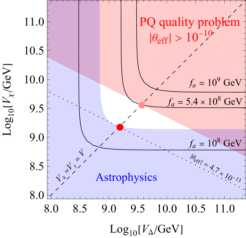
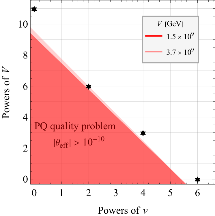
Figure 1: Left panel: Iso-contours of $f_{a}$ in the $(V_{\Delta},V_{\chi})$ plane. The red area signals the region of parameter space where the PQ quality problem arises, with $|\theta_{\rm eff}|>10^{-10}$. The blue area is disfavored by astrophysical bounds, $f_{a}\gtrsim 2.3\times 10^{8}\,\mathrm{GeV}$ (cf. Sect. 4.1). Along the dashed line, $V_{\Delta}=V_{\chi}\equiv V$ holds. Along the dotted line, $|\theta_{\rm eff}|$ acquires its minimal value compatible with astrophysical constraints. Right panel: Contribution to $|\theta_{\rm eff}|$ from operators whose projection on the VEVs is of the type $v^{m}V^{n}/\Lambda_{\rm UV}^{m+n-4}$, assuming $V_{\Delta}=V_{\chi}=V=3\sqrt{5}f_{a}$. In the red regions, $|\theta_{\rm eff}|>10^{-10}$ for the values of $V$ in the legend, which correspond color-wise to the red dots in the left panel. The black stars correspond to operators generated in our model which impose the strongest conditions for PQ quality, cf. Eq. (2.29).

In general, the PQ-breaking axion potential receives contributions both from high-scale ($V_{\Delta}$ and $V_{\chi}$) and EW scale ($v$) VEVs, and Eq. (2.26) generalizes to

$$\frac{v^{m}\;V_{\Delta}^{l}\;V_{\chi}^{n-l}}{\Lambda_{\rm UV}^{n+m-4}} \lesssim 10^{-10}\chi_{\rm QCD}^{4} \xrightarrow{V_{\chi}\sim V_{\Delta}\sim V} \frac{v^{m}\;V^{n}}{\Lambda_{\rm UV}^{n+m-4}} \lesssim 10^{-10}\chi_{\rm QCD}^{4}\,,$$ (2.27)

where the high-scale VEVs are related to $f_{a}$ via Eq. (2.24). Although only an admixture of the full EW VEV will be present in any $v$-type VEV, we can conservatively take the maximal value $v=246/\sqrt{2}\,\mathrm{GeV}$.

As discussed later in this section, our main result is that the model has dominant contributions to the axion potential of the form

$$\frac{V_{\Delta}^{5}\,V_{\chi}^{6}}{\Lambda_{\rm UV}^{7}}\,, \frac{v^{2}\,V_{\Delta}^{2}\,V_{\chi}^{4}}{\Lambda_{\rm UV}^{4}}\,, \frac{v^{4}\,V_{\Delta}\,V_{\chi}^{2}}{\Lambda_{\rm UV}^{3}}\,, \frac{v^{6}}{\Lambda_{\rm UV}^{2}}$$ (2.28)

$$\xrightarrow{V_{\chi}\sim V_{\Delta}\sim V} \frac{V^{11}}{\Lambda_{\rm UV}^{7}}\,, \frac{v^{2}\,V^{6}}{\Lambda_{\rm UV}^{4}}\,, \frac{v^{4}\,V^{3}}{\Lambda_{\rm UV}^{3}}\,, \frac{v^{6}}{\Lambda_{\rm UV}^{2}}\,,$$ (2.29)

which originate from the operators (and their Hermitian conjugates)

$$\Delta^{4}\Delta^{\ast}\chi^{*6}\,, \Phi^{2-k}\Sigma^{k}\Delta^{2}\chi^{*4}\,, \Phi^{4-k}\Sigma^{k}\Delta\chi^{*2}\,, \Phi^{4-k}\Sigma^{k}\Sigma^{2}\,,$$ (2.30)

respectively, for at least one integer value $k$. Given the values of $v$ and $\Lambda_{\rm UV}=M_{\rm Pl}$ stated above, the $d=8$ contribution in Eq. (2.28) (second one from the left) turns out to be the dominant one.

In the left panel of Fig. 1, we plot in red the region in the $V_{\Delta}$–$V_{\chi}$ plane where PQ quality is spoiled according to Eq. (2.27), with the leading contribution coming from $(m,l,n-l)=(2,2,4)$, i.e., the dimension $8$ operator in Eq. (2.30). The constraint from astrophysics (discussed in Sect. 4.1) on the other hand demands $f_{a}\gtrsim 2.3\times 10^{8}\,\mathrm{GeV}$, computed from the VEVs via Eq. (2.24), with the excluded region shown in blue. The allowed region which also solves the PQ quality problem is thus the white remainder, and the configuration optimizing the solution to the PQ quality problem is close to the diagonal line $V_{\chi}\sim V_{\Delta}\sim V\sim f_{a}$ and lies on the astrophysics boundary; it is marked with a darker red dot. The upper limit of the diagonal line is $f_{a}\lesssim 5.4\times 10^{8}\,\mathrm{GeV}$ and is marked by a lighter red dot. Off the dashed diagonal the admissible $f_{a}$ can be raised slightly further to $f_{a}=5.6\times 10^{8}\,\mathrm{GeV}$, corresponding to an unmarked point $(V_{\chi},V_{\Delta})\simeq(4.1,2.9)\times 10^{9}\,\mathrm{GeV}$.

The minimal value of $|\theta_{\rm eff}|$ sourced by the $d=8$ operator and allowed by astrophysical bounds is $|\theta^{\rm min}_{\rm eff}|\simeq 4.7\times 10^{-13}$, shown as a dotted line in the left panel of Fig. 1. This could be tested by future experiments measuring the neutron [49, 50] and proton [51] EDM, which are expected to improve the current sensitivity on $\theta_{\rm eff}$ by up to three orders of magnitude.

From now on we focus on the limit $V_{\Delta}\sim V_{\chi}\sim V$. The PQ quality constraint of Eq. (2.27) can then be plotted for a fixed value of $V$ in the plane of powers of $v$ and $V$, as shown in the right panel of Fig. 1. We show the quality constraint for two different values of $V$, corresponding to the maximal and minimal quality solutions from the left panel, where they are shown as dots of corresponding color. The light red region represents an enlargement of the forbidden darker region, while sufficient PQ-quality is achieved in the upper-right corner. The dominant contributions to the axion potential of Eq. (2.29) are shown as stars.

We now turn to the discussion of how the operators of Eq. (2.30) have been identified as the source of the dominant contribution to the axion potential. The salient points of discussion are given below:

• Each of the representations $\Delta$, $\chi$ or $\xi$ in an operator provides one power of $V$, while each of the irreps $\Phi$ or $\Sigma$ (generically labeling any copy of $\Phi^{\alpha}$ or $\Sigma^{\alpha}$) provides one power of $v$. All EW VEVs in the model originate from weak doublets, and hence an even power of them is needed to form an ${\rm SU}(2)_{L}$ invariant. A contribution $v^{m}V^{n}$ must thus necessarily come with $m$ being an even non-negative integer. Since $m\geq 6$ by itself already solves the quality issue, it is sufficient to identify the dominant contributions for $m=0,2,4,6$, which have been listed in Eq. (2.30) in matching order.

• The dominant contributions to the axion potential can be searched for in a systematic way:

  1. We first obtain a list of all invariants involving scalar fields of dimension $d$. We leverage external software, in particular GroupMath [52] and LiE [53], see App. B.2 for more details.

  2. We retain only invariants with a non-vanishing PQ charge, since only these can affect the axion potential.

  3. The list is refined further by demanding that an operator actually gives a non-vanishing vacuum contribution. This occurs only if the invariant contains an all-VEV term, i.e., a term in which every factor is a field with a non-vanishing VEV. This is hard to test for in an automated way, so we instead use a necessary (but not sufficient) condition: taking the VEV-directions in every factor of the invariant, the total charge of the product under any gauged $\mathrm{U}(1)$ must vanish. In the context of our setup, the pertinent test to perform is for the $B-L$ charge, which is part of ${\rm SU}(4)_{\rm PS}$.

  4. Having a fully refined list of operator candidates, we find those with the largest contributions $v^{m}V^{n}$ to the vacuum, and confirming their non-vanishing contribution by computing it explicitly. Both the refined list and the explicit confirmation of contributions are relegated to the Appendix, cf. App. B.3.1, while the final result of dominant operators has been given in Eq. (2.30).

• To further illuminate the resulting operators in Eq. (2.30), it is beneficial to build some intuition for which combinations of scalar fields of Table 1 can form an invariant. We list five rules an invariant must adhere to:

  • The total power of $\Phi$ and $\Sigma$ must be even (due to ${\rm SU}(2)_{L}$ invariance, as already described earlier).

  • The total power of $\chi$ and $\chi^{\ast}$ must be even (a restriction from the center of ${\rm SU}(2)_{R}$ combined with (i)).

  • The only non-trivial way a combination of $\Delta$ and $\chi$ enters is in powers of $\Delta\chi^{\ast 2}$ (a restriction from the center of ${\rm SU}(4)_{\rm PS}$).

  • The difference between the number of conjugated and un-conjugated irreps (counting $\Phi$, $\Sigma$, $\Delta$ and $\chi$ fields) must be divisible by $3$ (a restriction from the center of ${\rm SU}(3)_{f_{R}}$).

  • $\xi$ can usually be added with an arbitrary power, since it behaves as an adjoint or singlet under every group factor. In particular, it can usually also be omitted without jeopardizing the existence of the invariant.

  Given these considerations, the list of Eq. (2.30) could in fact be guessed, the only surprise is that a pure $V^{n}$ contribution arises only at $n=11$ and not at $n=9$. The invariant $\Delta^{3}\chi^{\ast 6}$ does in fact exists, but it does not contribute to the vacuum, and so the first $V^{n}$ contribution comes only after adding an additional $\Delta\Delta^{\ast}$ piece to it. This is a rather subtle result, which is discussed in more detail in App. B.3.1.

We conclude with the remark that the analysis of PQ quality in this section is based on a tree-level analysis of the effective theory, in which every operator is assumed to contribute via an (at most) $\mathcal{O}(1)$ dimensionless coefficient and a suppression with an appropriate power of $\Lambda_{\rm UV}$. It is an important, albeit often neglected point, that quantum corrections may in fact enhance operator contributions above those of the tree-level structural set-up; this is further elaborated on conceptually in App. B.3.2.

3 Reproducing the SM flavor structure

The fermions in our model consist of those in the SM, as well as the right-handed neutrinos and anomalons, introducing $3$ and $24$ new Weyl fermions, respectively. The right-handed neutrinos are in a flavor-triplet, while the anomalons form $8$ generations of flavor-antitriplets, cf. Table 1.

Since both right-handed neutrinos and anomalons are singlets under the SM group, they are also singlets in the EW broken phase ${\rm SU}(3)_{C}\times\mathrm{U}(1)_{\rm EM}$, thus mixing with left-handed neutrinos in the mass matrix. We analyze this complicated neutrino-anomalon sector in detail in Section 3.2, while we start the analysis with the simpler quark and charged-lepton sectors in Section 3.1.

3.1 Quark and charged-lepton sector

The operators from which the quark and charged-lepton mass matrices dominantly arise are the $Y^{\Phi^{\alpha}}_{I}$ and $Y^{\Sigma^{\alpha}}_{I}$ terms in Eq. (2.1). Note that these terms are renormalizable. Higher-order non-renormalizable operators will provide corrections, but they structurally connect the same fields as the renormalizable ones, hence their $V/\Lambda_{\rm UV}$ suppression yields only a numerically negligible correction. The analysis for quarks and charged leptons, unlike the neutrinos and anomalons, can thus be performed by considering the renormalizable operators only.

The requirements for a good fermion fit will dictate the needed number of copies of the scalar representations $\Phi$ and $\Sigma$ containing the SM Higgs, denoted by $N_{\Phi}$ and $N_{\Sigma}$, respectively. Since each type of operator with either $\Phi^{\alpha}$ or $\Sigma^{\alpha}$ comes with its own Clebsch-Gordan ratio between the down- and charged-lepton sectors, at least one of each type is required to avoid the bad mass relation $M_{D}\propto M_{E}^{T}$, hence $N_{\Phi},N_{\Sigma}\geq 1$. A further consideration on the number of copies comes from redundancies in the Yukawa matrices, namely rotations in family space and ${\rm SU}(3)_{f_{R}}$ gauge rotations. We shall discuss this in more detail in Sect. 3.3; for now it suffices to say that the minimal realistic setup requires at least $N_{\Phi}=1$ and $N_{\Sigma}=2$, since $N_{\Sigma}=1$ would enable a difference between the down- and charged-lepton sectors only in one family.

We focus below on the case $N_{\Phi}=1$ and $N_{\Sigma}=2$. Simplifying the notation $\{\Phi^{\alpha}\}_{\alpha=1}$ and $\{\Sigma^{\alpha}\}_{\alpha=1,2}$ from Eq. (2.1), we write the scalar representations simply as $\Phi$, $\Sigma$ and $\Sigma^{\prime}$, while the corresponding Yukawa couplings are denoted by $Y^{\Phi}_{I}$, $Y^{\Sigma}_{I}$ and $Y^{\Sigma^{\prime}}_{I}$, where the family index $I$ runs from $1$ to $3$. Each of the scalar irreps contains six SM weak doublets; three transform as $(1,2,+\tfrac{1}{2})$ and three transform as $(1,2,-\tfrac{1}{2})$ under the SM group, with the corresponding VEVs respectively equipped with the label $u$ or $d$, and the multiplicity of $3$ originating from these irreps being antitriplets under ${\rm SU}(3)_{f_{R}}$. Given the weak-doublet content of $\Phi$, $\Sigma$ and $\Sigma^{\prime}$ described above, we label their VEVs by the self-evident notation

$${\color[rgb]{0,0,1}v^{u\Phi}_{{\color[rgb]{0,0,0}A}}},\quad{\color[rgb]{0,0,1}v^{u\Sigma}_{{\color[rgb]{0,0,0}A}}},\quad{\color[rgb]{0,0,1}v^{u\Sigma^{\prime}}_{{\color[rgb]{0,0,0}A}}},\quad{\color[rgb]{0,0,1}v^{d\Phi}_{{\color[rgb]{0,0,0}A}}},\quad{\color[rgb]{0,0,1}v^{d\Sigma}_{{\color[rgb]{0,0,0}A}}},\quad{\color[rgb]{0,0,1}v^{d\Sigma^{\prime}}_{{\color[rgb]{0,0,0}A}}},$$ (3.1)

where $A$ is the flavor index. The EW VEVs (excluding the flavor indices that they carry) will be colored in blue for better visual clarity.

We relegate the bulk of the computational details to App. B.4, and here merely state the results. The up-quark ($U$), down-quark ($D$) and charged-lepton ($E$) mass matrices take the form

$$(M_{U})_{IA} =Y^{\Phi}_{I}{\color[rgb]{0,0,1}v^{u\Phi}_{{\color[rgb]{0,0,0}A}}}+Y^{\Sigma}_{I}{\color[rgb]{0,0,1}v^{u\Sigma}_{{\color[rgb]{0,0,0}A}}}+Y^{\Sigma^{\prime}}_{I}{\color[rgb]{0,0,1}v^{u\Sigma^{\prime}}_{{\color[rgb]{0,0,0}A}}},$$ (3.2)

$$(M_{D})_{IA} =Y^{\Phi}_{I}{\color[rgb]{0,0,1}v^{d\Phi}_{{\color[rgb]{0,0,0}A}}}+Y^{\Sigma}_{I}{\color[rgb]{0,0,1}v^{d\Sigma}_{{\color[rgb]{0,0,0}A}}}+Y^{\Sigma^{\prime}}_{I}{\color[rgb]{0,0,1}v^{d\Sigma^{\prime}}_{{\color[rgb]{0,0,0}A}}},$$ (3.3)

$$(M_{E})_{IA} =Y^{\Phi}_{I}{\color[rgb]{0,0,1}v^{d\Phi}_{{\color[rgb]{0,0,0}A}}}-3\,Y^{\Sigma}_{I}{\color[rgb]{0,0,1}v^{d\Sigma}_{{\color[rgb]{0,0,0}A}}}-3\,Y^{\Sigma^{\prime}}_{I}{\color[rgb]{0,0,1}v^{d\Sigma^{\prime}}_{{\color[rgb]{0,0,0}A}}},$$ (3.4)

where the LR convention was used, i.e. the Lagrangian contains terms

$$\mathcal{L}\supset-\sum_{I,A}(M_{U})_{IA}(\overline{u}_{L})^{I}(u_{R})^{A},$$ (3.5)

and analogously for other sectors. A choice of redundancy removal (see App. B.4), which yields a particularly transparent form for the mass matrices, is

$${\color[rgb]{0,0,1}v^{d\Sigma}_{{\color[rgb]{0,0,0}1}}}={\color[rgb]{0,0,1}v^{d\Sigma}_{{\color[rgb]{0,0,0}2}}}={\color[rgb]{0,0,1}v^{d\Sigma^{\prime}}_{{\color[rgb]{0,0,0}1}}} =0\,, Y^{\Sigma}_{1}=Y^{\Sigma}_{2}=Y^{\Sigma^{\prime}}_{1} =0\,,$$ (3.6)

resulting in the explicitly result

$$M_{U} =\left(\begin{smallmatrix}Y^{\Phi}_{1}{\color[rgb]{0,0,1}v^{u\Phi}_{{\color[rgb]{0,0,0}1}}}&Y^{\Phi}_{1}{\color[rgb]{0,0,1}v^{u\Phi}_{{\color[rgb]{0,0,0}2}}}&Y^{\Phi}_{1}{\color[rgb]{0,0,1}v^{u\Phi}_{{\color[rgb]{0,0,0}3}}}\\ Y^{\Phi}_{2}{\color[rgb]{0,0,1}v^{u\Phi}_{{\color[rgb]{0,0,0}1}}}+Y^{\Sigma^{\prime}}_{2}{\color[rgb]{0,0,1}v^{u\Sigma^{\prime}}_{{\color[rgb]{0,0,0}1}}}&Y^{\Phi}_{2}{\color[rgb]{0,0,1}v^{u\Phi}_{{\color[rgb]{0,0,0}2}}}+Y^{\Sigma^{\prime}}_{2}{\color[rgb]{0,0,1}v^{u\Sigma^{\prime}}_{{\color[rgb]{0,0,0}2}}}&Y^{\Phi}_{2}{\color[rgb]{0,0,1}v^{u\Phi}_{{\color[rgb]{0,0,0}3}}}+Y^{\Sigma^{\prime}}_{2}{\color[rgb]{0,0,1}v^{u\Sigma^{\prime}}_{{\color[rgb]{0,0,0}3}}}\\ Y^{\Phi}_{3}{\color[rgb]{0,0,1}v^{u\Phi}_{{\color[rgb]{0,0,0}1}}}+Y^{\Sigma}_{3}{\color[rgb]{0,0,1}v^{u\Sigma}_{{\color[rgb]{0,0,0}1}}}+Y^{\Sigma^{\prime}}_{3}{\color[rgb]{0,0,1}v^{u\Sigma^{\prime}}_{{\color[rgb]{0,0,0}1}}}&Y^{\Phi}_{3}{\color[rgb]{0,0,1}v^{u\Phi}_{{\color[rgb]{0,0,0}2}}}+Y^{\Sigma}_{3}{\color[rgb]{0,0,1}v^{u\Sigma}_{{\color[rgb]{0,0,0}2}}}+Y^{\Sigma^{\prime}}_{3}{\color[rgb]{0,0,1}v^{u\Sigma^{\prime}}_{{\color[rgb]{0,0,0}2}}}&Y^{\Phi}_{3}{\color[rgb]{0,0,1}v^{u\Phi}_{{\color[rgb]{0,0,0}3}}}+Y^{\Sigma}_{3}{\color[rgb]{0,0,1}v^{u\Sigma}_{{\color[rgb]{0,0,0}3}}}+Y^{\Sigma^{\prime}}_{3}{\color[rgb]{0,0,1}v^{u\Sigma^{\prime}}_{{\color[rgb]{0,0,0}3}}}\\ \end{smallmatrix}\right),$$ (3.7)

$$M_{D} =\left(\begin{smallmatrix}Y^{\Phi}_{1}{\color[rgb]{0,0,1}v^{d\Phi}_{{\color[rgb]{0,0,0}1}}}&Y^{\Phi}_{1}{\color[rgb]{0,0,1}v^{d\Phi}_{{\color[rgb]{0,0,0}2}}}&Y^{\Phi}_{1}{\color[rgb]{0,0,1}v^{d\Phi}_{{\color[rgb]{0,0,0}3}}}\\ Y^{\Phi}_{2}{\color[rgb]{0,0,1}v^{d\Phi}_{{\color[rgb]{0,0,0}1}}}&Y^{\Phi}_{2}{\color[rgb]{0,0,1}v^{d\Phi}_{{\color[rgb]{0,0,0}2}}}+Y^{\Sigma^{\prime}}_{2}{\color[rgb]{0,0,1}v^{d\Sigma^{\prime}}_{{\color[rgb]{0,0,0}2}}}&Y^{\Phi}_{2}{\color[rgb]{0,0,1}v^{d\Phi}_{{\color[rgb]{0,0,0}3}}}+Y^{\Sigma^{\prime}}_{2}{\color[rgb]{0,0,1}v^{d\Sigma^{\prime}}_{{\color[rgb]{0,0,0}3}}}\\ Y^{\Phi}_{3}{\color[rgb]{0,0,1}v^{d\Phi}_{{\color[rgb]{0,0,0}1}}}&Y^{\Phi}_{3}{\color[rgb]{0,0,1}v^{d\Phi}_{{\color[rgb]{0,0,0}2}}}+Y^{\Sigma^{\prime}}_{3}{\color[rgb]{0,0,1}v^{d\Sigma^{\prime}}_{{\color[rgb]{0,0,0}2}}}&Y^{\Phi}_{3}{\color[rgb]{0,0,1}v^{d\Phi}_{{\color[rgb]{0,0,0}3}}}+Y^{\Sigma}_{3}{\color[rgb]{0,0,1}v^{d\Sigma}_{{\color[rgb]{0,0,0}3}}}+Y^{\Sigma^{\prime}}_{3}{\color[rgb]{0,0,1}v^{d\Sigma^{\prime}}_{{\color[rgb]{0,0,0}3}}}\\ \end{smallmatrix}\right),$$ (3.8)

$$M_{E} =\left(\begin{smallmatrix}Y^{\Phi}_{1}{\color[rgb]{0,0,1}v^{d\Phi}_{{\color[rgb]{0,0,0}1}}}&Y^{\Phi}_{1}{\color[rgb]{0,0,1}v^{d\Phi}_{{\color[rgb]{0,0,0}2}}}&Y^{\Phi}_{1}{\color[rgb]{0,0,1}v^{d\Phi}_{{\color[rgb]{0,0,0}3}}}\\ Y^{\Phi}_{2}{\color[rgb]{0,0,1}v^{d\Phi}_{{\color[rgb]{0,0,0}1}}}&Y^{\Phi}_{2}{\color[rgb]{0,0,1}v^{d\Phi}_{{\color[rgb]{0,0,0}2}}}-3Y^{\Sigma^{\prime}}_{2}{\color[rgb]{0,0,1}v^{d\Sigma^{\prime}}_{{\color[rgb]{0,0,0}2}}}&Y^{\Phi}_{2}{\color[rgb]{0,0,1}v^{d\Phi}_{{\color[rgb]{0,0,0}3}}}-3Y^{\Sigma^{\prime}}_{2}{\color[rgb]{0,0,1}v^{d\Sigma^{\prime}}_{{\color[rgb]{0,0,0}3}}}\\ Y^{\Phi}_{3}{\color[rgb]{0,0,1}v^{d\Phi}_{{\color[rgb]{0,0,0}1}}}&Y^{\Phi}_{3}{\color[rgb]{0,0,1}v^{d\Phi}_{{\color[rgb]{0,0,0}2}}}-3Y^{\Sigma^{\prime}}_{3}{\color[rgb]{0,0,1}v^{d\Sigma^{\prime}}_{{\color[rgb]{0,0,0}2}}}&Y^{\Phi}_{3}{\color[rgb]{0,0,1}v^{d\Phi}_{{\color[rgb]{0,0,0}3}}}-3Y^{\Sigma}_{3}{\color[rgb]{0,0,1}v^{d\Sigma}_{{\color[rgb]{0,0,0}3}}}-3Y^{\Sigma^{\prime}}_{3}{\color[rgb]{0,0,1}v^{d\Sigma^{\prime}}_{{\color[rgb]{0,0,0}3}}}\\ \end{smallmatrix}\right).$$ (3.9)

The parameter values $Y^{\Sigma}_{3}$ and $Y^{\Sigma^{\prime}}_{2}$, as well as the EW VEVs ${\color[rgb]{0,0,1}v^{d\Sigma}_{{\color[rgb]{0,0,0}3}}}$ and ${\color[rgb]{0,0,1}v^{d\Sigma^{\prime}}_{{\color[rgb]{0,0,0}2}}}$, can be taken to be real without loss of generality.

The advantage of the choice in Eq. (3.6) is that the mass matrices for the $D$ and $E$ sectors become as simple as possible, allowing to scrutinize whether the $D$ and $E$ masses can be made sufficiently different. The main driver are the $\Sigma$ and $\Sigma^{\prime}$ terms, due to the Clebsch coefficient $-3$ for charged leptons. Eqs. (3.7)–(3.9) should yield a realistic Yukawa sector, with further justification given in Sect. 3.3.

3.2 The neutrino-anomalon sector

Under ${\rm SU}(3)_{C}\times\mathrm{U}(1)_{\rm EM}$, the left-handed neutrinos $(\overline{\nu}_{L})^{I}$, right-handed neutrinos $(\nu_{R})^{A}$, and anomalons $(\Psi_{R})^{K}{}_{A}$ are all singlets, hence they mix in the mass matrix. In short-hand notation, we shall refer to them by $L$, $R$ and $\Psi$, respectively.

The index $I$ is a family index originating from $Q_{L}$, $A$ is a flavor index (for ${\rm SU}(3)_{f_{R}}$), while $K$ denotes the anomalon multiplicity index; $I,A\in\{1,2,3\}$ while $K\in\{1,\ldots,8\}$. Note that anomalons carry two types of indices and the full space of considered fields $L\oplus R\oplus\Psi$ has dimension $3+3+8\times 3=30$.

The incorporation of anomalons into the neutrino sector greatly complicates the analysis, more so since of the $24$ (dominantly) anomalon states $8$ turn out to have a parametrically smaller mass, and thus special care is needed to consider them properly. To improve the clarity of presentation, we shall split our considerations into two parts: the neutrino-anomalon mass matrix is presented and discussed in Sect. 3.2.1, while the resulting spectrum and mixing are analyzed in Sect. 3.2.2; the derivation and computational details are relegated to App. B.4.

In order to avoid confusion in terminology between the flavor and mass eigenstates of this sector, we explicitly state our naming convention already now at the onset:

• The flavor states $L\oplus R\oplus\Psi$ are referred to as L-neutrinos, R-neutrinos and anomalons.

• The mass eigenstates which contain a dominant admixture of the above flavor eigenstates are in order named active neutrinos, sterile neutrinos and massive anomalons. Anticipating the $24=16+8$ parametric split in the latter’s masses, we dub the two respective groups heavy anomalons and light anomalons.

3.2.1 The neutrino-anomalon mass matrix

The neutrino-anomalon mass matrix can be written in block form using the basis split $L\oplus R\oplus\Psi$:

$$\mathcal{L} \supset\frac{1}{2}\,\begin{pmatrix}(\overline{\nu}_{L})^{I}\\[2.0pt] (\nu_{R})^{A}\\[2.0pt] (\Psi_{R})^{K}{}_{A}\\ \end{pmatrix}^{T}\begin{pmatrix}(M_{LL})_{IJ}&(M_{LR})_{IB}&(M_{L\Psi})_{IN}{}^{B}\\[2.0pt] (M_{RL})_{AJ}&(M_{RR})_{AB}&(M_{R\Psi})_{AN}{}^{B}\\[2.0pt] (M_{\Psi L})_{K}{}^{A}{}_{J}&(M_{\Psi R})_{K}{}^{A}{}_{B}&(M_{\Psi\Psi})_{K}{}^{A}{}_{N}{}^{B}\\ \end{pmatrix}\begin{pmatrix}(\overline{\nu}_{L})^{J}\\[2.0pt] (\nu_{R})^{B}\\[2.0pt] (\Psi_{R})^{N}{}_{B}\\ \end{pmatrix}\,.$$ (3.10)

Each block carries the appropriate type of indices for the fields it connects. The double index notation of the basis of anomalons carries over to all anomalon-related blocks, e.g. $M_{\Psi\Psi}$ has $4$ indices.

The first step in the determination of each block is to identify the operators which contribute in a relevant way. The list of sources, along with the label for its corresponding coefficient, is conveniently compiled in Table 2. This is a non-trivial result, which requires careful consideration of a number of subtleties, which we are about to discuss. With the computational details of each contribution relegated to App. B.4, we directly state here the final result:

$$(M_{LL})_{IJ} \approx 0\,,$$ (3.11)

$$(M_{LR})_{IB} =Y^{\Phi}_{I}\,{\color[rgb]{0,0,1}v^{u\Phi}_{{\color[rgb]{0,0,0}B}}}-3\,Y^{\Sigma}_{I}\,{\color[rgb]{0,0,1}v^{u\Sigma}_{{\color[rgb]{0,0,0}B}}}-3\,Y^{\Sigma^{\prime}}_{I}\,{\color[rgb]{0,0,1}v^{u\Sigma^{\prime}}_{{\color[rgb]{0,0,0}B}}}\,,$$ (3.12)

$$(M_{RR})_{AB} =Y_{R}\,{\color[rgb]{1.0,0,0}Z^{\ast}_{{\color[rgb]{0,0,0}AB}}}\,,$$ (3.13)

$$(M_{L\Psi})_{IN}{}^{B} =\frac{1}{\Lambda_{\rm UV}}\,\epsilon^{BCD}\,{\color[rgb]{1.0,0,0}V}_{C}\,\left(\mathcal{A}_{IN}\,{\color[rgb]{0,0,1}v^{u\Phi}_{{\color[rgb]{0,0,0}D}}}-3\,\mathcal{B}_{IN}\,{\color[rgb]{0,0,1}v^{u\Sigma}_{{\color[rgb]{0,0,0}D}}}-3\,\mathcal{B}^{\prime}_{IN}\,{\color[rgb]{0,0,1}v^{u\Sigma^{\prime}}_{{\color[rgb]{0,0,0}D}}}\right)$$

$$\quad+\frac{1}{\Lambda_{\rm UV}^{2}}\;{\color[rgb]{1.0,0,0}Z^{{\color[rgb]{0,0,0}BC}}}\,\left(\tilde{\mathcal{A}}_{IN}\,({\color[rgb]{0,0,1}v^{\ast u\Phi}})^{{\color[rgb]{0,0,0}D}}+\tilde{\mathcal{B}}_{IN}\,({\color[rgb]{0,0,1}v^{\ast u\Sigma}})^{{\color[rgb]{0,0,0}D}}+\tilde{\mathcal{B}}^{\prime}_{IN}\,({\color[rgb]{0,0,1}v^{\ast u\Sigma^{\prime}}})^{{\color[rgb]{0,0,0}D}}\right)\,{\color[rgb]{1.0,0,0}V^{\ast}}{}^{E}\,\epsilon_{CDE}\,,$$ (3.14)

$$(M_{R\Psi})_{AN}{}^{B} =\frac{\mathcal{C}_{N}}{\Lambda_{\rm UV}}\,\epsilon^{BCD}{\color[rgb]{1.0,0,0}Z^{\ast}_{{\color[rgb]{0,0,0}AC}}}\,{\color[rgb]{1.0,0,0}V}_{D}+\frac{\tilde{\mathcal{C}}_{N}}{\Lambda_{\rm UV}^{3}}\;{\color[rgb]{1.0,0,0}Z^{{\color[rgb]{0,0,0}EF}}}\,{\color[rgb]{1.0,0,0}Z^{\ast}_{{\color[rgb]{0,0,0}ED}}}\,{\color[rgb]{1.0,0,0}Z^{\ast}_{{\color[rgb]{0,0,0}AC}}}\,{\color[rgb]{1.0,0,0}V}_{F}\;\epsilon^{BCD}\,,$$ (3.15)

$$(M_{\Psi\Psi})_{K}{}^{A}{}_{N}{}^{B} =\frac{\mathcal{D}_{KN}}{\Lambda_{\rm UV}^{2}}\,\epsilon^{ACD}\,\epsilon^{BEF}{\color[rgb]{1.0,0,0}Z^{\ast}_{{\color[rgb]{0,0,0}CE}}}\,{\color[rgb]{1.0,0,0}V}_{D}\,{\color[rgb]{1.0,0,0}V}_{F}$$

$$\quad+\frac{\tilde{\mathcal{D}}_{KN}}{\Lambda_{\rm UV}}\left({\color[rgb]{0,0,1}v^{u\Phi}}^{\ast A}{\color[rgb]{0,0,1}v^{d\Phi}}^{\ast B}+{\color[rgb]{0,0,1}v^{d\Phi}}^{\ast A}{\color[rgb]{0,0,1}v^{u\Phi}}^{\ast B}\right)$$

$$\quad+\frac{\tilde{\mathcal{E}}_{KN}}{\Lambda_{\rm UV}}\left({\color[rgb]{0,0,1}v^{u\Sigma}}^{\ast A}{\color[rgb]{0,0,1}v^{d\Sigma}}^{\ast B}+{\color[rgb]{0,0,1}v^{d\Sigma}}^{\ast A}{\color[rgb]{0,0,1}v^{u\Sigma}}^{\ast B}\right)$$

$$\quad+\left(\frac{1}{2}\,\frac{\tilde{\mathcal{E}}^{\prime}_{KN}}{\Lambda_{\rm UV}}\left({\color[rgb]{0,0,1}v^{u\Sigma}}^{\ast A}{\color[rgb]{0,0,1}v^{d\Sigma^{\prime}}}^{\ast B}+{\color[rgb]{0,0,1}v^{d\Sigma}}^{\ast A}{\color[rgb]{0,0,1}v^{u\Sigma^{\prime}}}^{\ast B}\right)+\left[{}^{K\leftrightarrow N}_{A\leftrightarrow B}\right]\right)$$

$$\quad+\frac{\tilde{\mathcal{E}}^{\prime\prime}_{KN}}{\Lambda_{\rm UV}}\left({\color[rgb]{0,0,1}v^{u\Sigma^{\prime}}}^{\ast A}{\color[rgb]{0,0,1}v^{d\Sigma^{\prime}}}^{\ast B}+{\color[rgb]{0,0,1}v^{d\Sigma^{\prime}}}^{\ast A}{\color[rgb]{0,0,1}v^{u\Sigma^{\prime}}}^{\ast B}\right)$$

$$\quad+\frac{\tilde{\mathcal{F}}_{KN}}{\Lambda^{4}_{\rm UV}}\;{\color[rgb]{1.0,0,0}Z^{{\color[rgb]{0,0,0}GH}}}\,{\color[rgb]{1.0,0,0}Z^{\ast}_{{\color[rgb]{0,0,0}CE}}}\,{\color[rgb]{1.0,0,0}Z^{\ast}_{{\color[rgb]{0,0,0}DF}}}\,{\color[rgb]{1.0,0,0}V}_{G}\,{\color[rgb]{1.0,0,0}V}_{H}\;\epsilon^{ACD}\epsilon^{BEF}$$

$$\quad+\frac{\tilde{\mathcal{G}}_{KN}}{\Lambda^{4}_{\rm UV}}\;{\color[rgb]{1.0,0,0}Z^{{\color[rgb]{0,0,0}GH}}}\,{\color[rgb]{1.0,0,0}Z^{\ast}_{{\color[rgb]{0,0,0}CE}}}\,{\color[rgb]{1.0,0,0}Z^{\ast}_{{\color[rgb]{0,0,0}DG}}}\,{\color[rgb]{1.0,0,0}V}_{F}\,{\color[rgb]{1.0,0,0}V}_{H}\;\epsilon^{ABC}\epsilon^{DEF}\,.$$ (3.16)

We remind the reader of our color coding: red for the Pati-Salam braking scale, and blue for the EW scale VEVs. The neutrino-anomalon mass matrix is symmetric, implying

$$(M_{RL})_{AJ} =(M_{LR})_{JA}\,, (M_{\Psi L})_{K}{}^{A}{}_{J} =(M_{L\Psi})_{JK}{}^{A}\,,$$

$$(M_{\Psi R})_{K}{}^{A}{}_{B} =(M_{R\Psi})_{BK}{}^{A}\,, (M_{\Psi\Psi})_{K}{}^{A}{}_{N}{}^{B} =(M_{\Psi\Psi})_{N}{}^{B}{}_{K}{}^{A}\,,$$ (3.17)

from where the remaining blocks (below the diagonal) can be determined.

type	operator $\mathcal{O}$	$d$	$\langle M_{\mathcal{O}}\rangle$	$\#$ of $\mathcal{O}$	coefficients
$LL$	$\overline{Q}_{L}\overline{Q}_{L}\,\Delta(\Phi^{2}+\Phi\Sigma+\Sigma^{2})$	$6$	$v^{2}V/\Lambda_{\rm UV}^{2}$	$1+2+5$	—
$LR$	$\overline{Q}_{L}Q_{R}\,(\Phi+\Sigma+\Sigma^{\prime})$	$4$	$v$	$1+1+1$	$Y^{\Phi}_{I}$, $Y^{\Sigma}_{I}$,$Y^{\Sigma^{\prime}}_{I}$
$RR$	$Q_{R}Q_{R}\,\Delta^{\ast}$	$4$	$V$	$1$	$Y_{R}$
$L\Psi$	$\overline{Q}_{L}\Psi_{R}\,\chi(\Phi+\Sigma+\Sigma^{\prime})$	$5$	$vV/\Lambda_{\rm UV}$	$1+1+1$	$\mathcal{A}_{IN}$, $\mathcal{B}_{IN}$, $\mathcal{B}^{\prime}_{IN}$
$L\Psi$	$\overline{Q}_{L}\Psi_{R}\,\Delta\chi^{*}(\Phi^{*}+\Sigma^{*}+\Sigma^{\prime*})$	$6$	$vV^{2}/\Lambda_{\rm UV}^{2}$	$1+2+2$	$\tilde{\mathcal{A}}_{IN}$, $\tilde{\mathcal{B}}_{IN}$, $\tilde{\mathcal{B}}^{\prime}_{IN}$
$R\Psi$	$Q_{R}\Psi_{R}\,\Delta^{\ast}\chi$	$5$	$V^{2}/\Lambda_{\rm UV}$	$1$	$\mathcal{C}_{N}$
$R\Psi$	$Q_{R}\Psi_{R}\Delta\Delta^{*2}\chi$	$7$	$V^{4}/\Lambda_{\rm UV}^{3}$	$56$	$\tilde{\mathcal{C}}_{N}$
$\Psi\Psi$	$\Psi_{R}\Psi_{R}\,\Delta^{\ast}\chi^{2}$	$6$	$V^{3}/\Lambda_{\rm UV}^{2}$	$1$	$\mathcal{D}_{(KN)}$
$\Psi\Psi$	$\Psi_{R}\Psi_{R}\,\Phi^{\ast 2}$	$5$	$v^{2}/\Lambda_{\rm UV}$	$1$	$\tilde{\mathcal{D}}_{(KN)}$
$\Psi\Psi$	$\Psi_{R}\Psi_{R}\,(\Sigma^{\ast 2}+\Sigma^{\ast}\Sigma^{\prime\ast}+\Sigma^{\prime\ast 2})$	$5$	$v^{2}/\Lambda_{\rm UV}$	$1+1+1$	$\tilde{\mathcal{E}}_{(KN)},\tilde{\mathcal{E}}^{\prime}_{KN},\tilde{\mathcal{E}}^{\prime\prime}_{(KN)}$
$\Psi\Psi$	$\Psi_{R}\Psi_{R}\Delta\Delta^{*2}\chi^{2}$	$8$	$V^{5}/\Lambda_{\rm UV}^{4}$	$42$	$\tilde{\mathcal{F}}_{(KN)},\tilde{\mathcal{G}}_{[KN]}$

Table 2: List of the operators contributing to the neutrino-anomalon mass matrix in a relevant way. The operators $\mathcal{O}$ are arranged according to type, i.e. which block in the basis $L\oplus R\oplus\Psi$ they contribute to. For each operator we also give its mass dimension $d$, its contribution $\langle M_{\mathcal{O}}\rangle$ to the mass in terms of VEVs ($v$ and $V$ are the EW and PS-breaking VEVs, respectively), the number $\#$ of independent invariants (index contractions) of the involved fields, and finally the labeling of coefficients. The subdominant contributions have a tilde in the coefficient label.

The main points to note about this result are the following:

1. Regarding the coefficients:

   • For every block entry all dominant contributions are provided, while for anomalon-related blocks we also add certain subdominant contributions, which as we shall later see are critical for describing the light anomalons. The coefficients of subdominant contributions are labeled with a tilde, while primes are used when $\Sigma$-irreps are replaced by $\Sigma^{\prime}$ in an operator.

   • All coefficients in Table 2 are complex, with $I\in\{1,\ldots,3\}$ denoting $Q_{L}$-family indices and $K,N\in\{1,\ldots,8\}$ $\Psi$-family indices. The (anti-)symmetry of matrix coefficients is denoted in Table 2 by parenthesis (square brackets). The parameter $Y_{R}$ has no indices and is simply a complex number.

2. Determining the dominant contributions:

   • For each block in Eq. (3.10), we identify the dominant contribution of the form $v^{m}V^{n}/\Lambda_{\rm UV}^{m+n-1}$ by listing all operators up to dimension $d=9$ involving the relevant fermion fields (using the methods described in App. B.2), and ordering them according to the size of their contribution. We assume the VEV scales as

     $$v \sim 10^{2}\,\mathrm{GeV}\,, V \in[10^{9},10^{14}]\,\mathrm{GeV}\,, \Lambda_{\rm UV} \sim M_{\rm Pl}\sim 10^{19}\,\mathrm{GeV}\,,$$ (3.18)

     where importantly we do not commit to a predetermined scale $V$. We instead consider a broader range of interesting scenarios, from the $V=10^{9}\,\mathrm{GeV}$ high-quality PQ symmetry scenario (according to Sect. 2.3) on the lower end, to $V=10^{14}\,\mathrm{GeV}$ on the higher end (this value being set by the upper bound on the seesaw scale — cf. also Sect. 4.3). This range of $V$ is of interest both for axion phenomenology and anomalon cosmology, cf. Sect. 4 and Sect. 5, respectively.

   • Regardless of choice of $V$ in Eq. (3.18), it turns out that dominant operators can always be identified unambiguously. This is not the case for all subdominant operators: a comparison of $\tilde{\mathcal{D}}$- and $\tilde{\mathcal{E}}$-contributions to those of $\tilde{\mathcal{F}}$-type show that the former are larger at small $V$, and the latter at large $V$. Furthermore, the operators (as specified by field powers) yielding dominant contributions always have a single independent contraction in their gauge indices, thereby requiring only one coefficient label for each. This is unlike some subdominant contributions with $\#>1$ in Table 2, which in any case require an altogether different treatment. Finally, one has to take care in determining the dominant contribution: due to the involvement of two scales, namely $v$ and $V$, the dominant contributions in a block entry are not always those of lowest dimension $d$. In the $\Psi\Psi$-block, the $d(\mathcal{D})=6$ is larger than the subdominant case with $d(\tilde{\mathcal{D}})=5$.

   • The $M_{LL}$ block is parametrically small, so we set it to zero in Eq. (3.11) — hence no associated coefficient in Table 2. The blocks $M_{RR}$ and $M_{LR}$ have the renormalizable Majorana and Dirac contributions, respectively, as in type-I seesaw; they are renormalizable contributions from Eq. (2.1). The block $M_{LR}$ takes an analogous form to $M_{U,D,E}$ in Eqs. (3.7)–(3.9) and with the redundancy-removal ansatz of Eq. (3.6) takes the explicit form

     $$M_{LR} =\left(\begin{smallmatrix}Y^{\Phi}_{1}{\color[rgb]{0,0,1}v^{u\Phi}_{{\color[rgb]{0,0,0}1}}}&Y^{\Phi}_{1}{\color[rgb]{0,0,1}v^{u\Phi}_{{\color[rgb]{0,0,0}2}}}&Y^{\Phi}_{1}{\color[rgb]{0,0,1}v^{u\Phi}_{{\color[rgb]{0,0,0}3}}}\\ Y^{\Phi}_{2}{\color[rgb]{0,0,1}v^{u\Phi}_{{\color[rgb]{0,0,0}1}}}-3Y^{\Sigma^{\prime}}_{2}{\color[rgb]{0,0,1}v^{u\Sigma^{\prime}}_{{\color[rgb]{0,0,0}1}}}&Y^{\Phi}_{2}{\color[rgb]{0,0,1}v^{u\Phi}_{{\color[rgb]{0,0,0}2}}}-3Y^{\Sigma^{\prime}}_{2}{\color[rgb]{0,0,1}v^{u\Sigma^{\prime}}_{{\color[rgb]{0,0,0}2}}}&Y^{\Phi}_{2}{\color[rgb]{0,0,1}v^{u\Phi}_{{\color[rgb]{0,0,0}3}}}-3Y^{\Sigma^{\prime}}_{2}{\color[rgb]{0,0,1}v^{u\Sigma^{\prime}}_{{\color[rgb]{0,0,0}3}}}\\ Y^{\Phi}_{3}{\color[rgb]{0,0,1}v^{u\Phi}_{{\color[rgb]{0,0,0}1}}}-3Y^{\Sigma}_{3}{\color[rgb]{0,0,1}v^{u\Sigma}_{{\color[rgb]{0,0,0}1}}}-3Y^{\Sigma^{\prime}}_{3}{\color[rgb]{0,0,1}v^{u\Sigma^{\prime}}_{{\color[rgb]{0,0,0}1}}}&Y^{\Phi}_{3}{\color[rgb]{0,0,1}v^{u\Phi}_{{\color[rgb]{0,0,0}2}}}-3Y^{\Sigma}_{3}{\color[rgb]{0,0,1}v^{u\Sigma}_{{\color[rgb]{0,0,0}2}}}-3Y^{\Sigma^{\prime}}_{3}{\color[rgb]{0,0,1}v^{u\Sigma^{\prime}}_{{\color[rgb]{0,0,0}2}}}&Y^{\Phi}_{3}{\color[rgb]{0,0,1}v^{u\Phi}_{{\color[rgb]{0,0,0}3}}}-3Y^{\Sigma^{\prime}}_{3}{\color[rgb]{0,0,1}v^{u\Sigma^{\prime}}_{{\color[rgb]{0,0,0}3}}}-3Y^{\Sigma}_{3}{\color[rgb]{0,0,1}v^{u\Sigma}_{{\color[rgb]{0,0,0}3}}}\\ \end{smallmatrix}\right)\,.$$ (3.19)

     All contributions in anomalon-related blocks of Eqs. (3.14)–(3.16) come, however, from non-renormalizable operators; for further explicit details, see App. B.4.

3. The need for subdominant contributions — a split in the massive-anomalon spectrum:

   • Suppose we switch on only the dominant contributions in the anomalon-related blocks of Eqs. (3.14)–(3.16). Then the $30\times 30$ mass matrix of Eq. (3.10) has $8$ massless modes. These massless anomalon modes are related to the direction of the VEV of $\chi$ in flavor space: ${\color[rgb]{1.0,0,0}V}_{A}$. Explicitly, defining

     $$(\Psi_{0})^{K}{}_{A} =\mathcal{N}^{K}\,{\color[rgb]{1.0,0,0}V}_{A}\,,$$ (3.20)

     for arbitrary coefficients $\mathcal{N}^{K}$ (hence $8$ such independent states), it is easily seen that by retaining only dominant terms (which we abbreviate by $\tilde{\mathcal{X}}\to 0$) we have

     $$(M_{L\Psi})_{IN}{}^{B}\Big{|}_{\tilde{\mathcal{X}}\to 0}\,(\Psi_{0})^{N}{}_{B} =0\,,$$ (3.21)

     $$(M_{R\Psi})_{AN}{}^{B}\Big{|}_{\tilde{\mathcal{X}}\to 0}\,(\Psi_{0})^{N}{}_{B} =0\,,$$ (3.22)

     $$(M_{\Psi\Psi})_{K}{}^{A}{}_{N}{}^{B}\Big{|}_{\tilde{\mathcal{X}}\to 0}\,(\Psi_{0})^{N}{}_{B} =0\,,$$ (3.23)

     hence $(0,0,\Psi_{0})$ are null eigenmodes of the full neutrino-anomalon mass matrix of Eq. (3.10). Indeed, the reason for the massless anomalon modes in the $\langle\chi\rangle$-direction is that all dominant operators form invariants, in which the flavor indices of anomalons and the actual VEV $\langle\chi\rangle={\color[rgb]{1.0,0,0}V}_{A}$ are contracted through the 3D Levi-Civita tensor, see expressions for non-tilde contributions in Eqs. (3.14)–(3.16). This is apparently an accidental feature in our model.

   • The $\Psi_{0}$ direction is properly described only once contributions beyond the dominant ones are considered. Crucially, the tilde contributions are those, which contribute dominantly to the $\Psi_{0}$ direction. Their derivation is sufficiently subtle that we have relegated it to App. B.4. Since the tilde contributions are subdominant in directions orthogonal to $\Psi_{0}$, there is a split in the massive-anomalon spectrum. Note, however, that in the presence of subdominant contributions, $\Psi_{0}$ is no longer an exact eigenmode; the light anomalons align close to (but not exactly in) the $\Psi_{0}$ direction, while heavy anomalons align closely along directions orthogonal to $\Psi_{0}$. In conclusion, the contributions in Eqs. (3.11)–(3.16) thus properly describe, to parametrically leading order, the entire space of states in the neutrino-anomalon sector.

3.2.2 Understanding the neutrino-anomalon spectrum and mixing

We now turn to analyzing the masses and mixings in the neutrino-anomalon sector. Although Eqs. (3.11)–(3.16) provide a complete description of the $30\times 30$ mass matrix of Eq. (3.10) up to parametrically leading order, we aim for a simplified analytic understanding of its features.

A convenient approach is to start with the block split $L\oplus R\oplus\Psi$, and then take into account the additional heavy-light split in the anomalon sector. Splitting the space $\Psi=\Psi_{0}\oplus\Psi_{\perp}$ (with a rotation relative to the original basis $\Psi^{K}{}_{A}$), where $\Psi_{\perp}$ represents the orthogonal complement in $\Psi$-space of the directions $\Psi_{0}$, we obtain the basis $L\oplus R\oplus\Psi_{\perp}\oplus\Psi_{0}$ ($3+3+16+8$ in dimensions), in which the mass matrix can be parametrically written as

$$\begin{pmatrix}M_{LL}&M_{LR}&M_{L\Psi_{\perp}}&M_{L\Psi_{0}}\\ M_{RL}&M_{RR}&M_{R\Psi_{\perp}}&M_{R\Psi_{0}}\\ M_{\Psi_{\perp}L}&M_{\Psi_{\perp}R}&M_{\Psi_{\perp}\Psi_{\perp}}&M_{\Psi_{\perp}\Psi_{0}}\\ M_{\Psi_{0}L}&M_{\Psi_{0}R}&M_{\Psi_{0}\Psi_{\perp}}&M_{\Psi_{0}\Psi_{0}}\\ \end{pmatrix} \sim\begin{pmatrix}\tfrac{v^{2}V}{\Lambda_{\rm UV}^{2}}&yv&l\,\tfrac{vV}{\Lambda_{\rm UV}}&\tilde{l}\,\tfrac{vV^{2}}{\Lambda_{\rm UV}^{2}}\\[3.0pt] ..&V&r\,\tfrac{V^{2}}{\Lambda_{\rm UV}}&\tilde{r}\,\tfrac{V^{4}}{\Lambda_{\rm UV}^{3}}\\[3.0pt] ..&..&\tfrac{V^{3}}{\Lambda_{\rm UV}^{2}}&\tfrac{v^{2}}{\Lambda_{\rm UV}}+\tfrac{V^{5}}{\Lambda_{\rm UV}^{4}}\\[3.0pt] ..&..&..&\tfrac{v^{2}}{\Lambda_{\rm UV}}+\tfrac{V^{5}}{\Lambda_{\rm UV}^{4}}\\ \end{pmatrix}\,,$$ (3.24)

where the entries denoted by dots are filled-in so that the matrix is symmetric. The VEVs $V$ and $v$, along with the UV scale $\Lambda_{\rm UV}$, take the values from Eq. (3.18), and the parametric sizes of each entry have been looked up in Table 2. We omit the coefficients; we assume they are order one in anomalon-only blocks, but their effect in off-diagonal blocks mixing anomalons and neutrinos is mimicked by the parameters $\{l,r,\tilde{l},\tilde{r}\}$. Finally, $y$ represents the Yukawa coupling; assuming the interference from mixing terms with anomalons is subdominant, the correct mass range for active neutrinos $m_{\nu}\sim 0.1\,\mathrm{eV}$ is automatically obtained by expressing $y$ from the seesaw formula:

$$y \sim\sqrt{m_{\nu}V/v^{2}}\,.$$ (3.25)

A seesaw scale $V=10^{9}\,\mathrm{GeV}$ is rather low, so we get a suppression from $y\sim 10^{-2.5}$, while the ideal seesaw scale $V=10^{14}\,\mathrm{GeV}$ yields $y\sim 1$.

To reiterate the connection of the $4\times 4$ block form with the explicit terms in Eqs. (3.11)–(3.16), note that switching off the tilde (subdominant) terms results in the last row and column in Eq. (3.24) vanishing, since the dominant terms do not connect to $\Psi_{0}$. Switching on the tilde terms induces contributions to both the $\Psi_{0}$ and $\Psi_{\perp}$ rows/columns, but we omit writing them for the latter case since the dominant contributions there are already parametrically larger. In particular, the $\tilde{\mathcal{D}},\tilde{\mathcal{E}},\tilde{\mathcal{F}}$-type contributions are present in all $\Psi\Psi$-blocks, i.e. the entire bottom-right $2\times 2$ part of the block matrix.

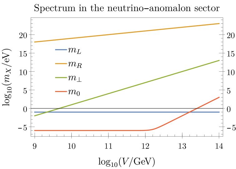
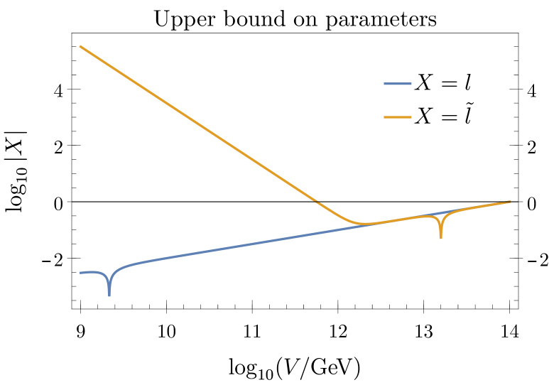
Figure 2: The spectrum of neutrinos and anomalons as a function of the Pati-Salam breaking scale $V$ (left panel), and the upper bounds on parameters $l$ and $\tilde{l}$ from Eq. (3.30) and (3.31) for mixing not to interfere with the spectrum approximation (right panel).

Given the hierarchical nature of the $4\times 4$ mass matrix in Eq. (3.24), we can apply perturbative methods in its analysis, see App. B.4 for a quick overview. Assuming a small enough interference from off-diagonal couplings other than $M_{LR}$ — to be quantified later — the mass eigenvalues are simply the diagonal entries (except $m_{L}$ coming from the seesaw formula):

$$m_{L} \sim\frac{y^{2}v^{2}}{V}\sim m_{\nu}\,, m_{R} \sim V\,, m_{\perp} \sim\frac{V^{3}}{\Lambda_{\rm UV}^{2}}\,, m_{0} \sim\frac{v^{2}}{\Lambda_{\rm UV}}+\frac{V^{5}}{\Lambda_{\rm UV}^{4}}\,.$$ (3.26)

Given the VEV and parameter values in Eq. (3.18) and (3.25), the following hierarchies become apparent:

$$m_{L},m_{\perp},m_{0} \ll m_{R}\,, m_{0} \ll m_{\perp}\,.$$ (3.27)

The only ambiguity is how the active neutrino mass $m_{L}$ is placed relative to anomalon masses $m_{0}$ and $m_{\perp}$. We plot the eigenvalues as functions of the PS-breaking scale $V$ in the left panel of Fig. 2. We see that in the given range of scale $V$, heavy anomalons have masses between $0.01\,\mathrm{eV}$ and $10\,\mathrm{TeV}$, while light anomalons are between $1\,\mathrm{\mu eV}$ and $1\,\mathrm{keV}$.

The approximate expressions in Eq. (3.26) are valid as long as that quantity dominates in the approximation for $m_{i}$, cf. Eq. (B.45) in the Appendix. Since $m_{R}\approx M_{RR}$ is very large, terms involving this quantity are negligible, so we get the main restrictions in the form

$$M_{L\perp}^{2} \ll m_{L}\,|m_{L}-m_{\perp}|\,, M_{L0}^{2} \ll m_{L}\,|m_{L}-m_{0}|\,,$$ (3.28)

$$M_{L\perp}^{2} \ll m_{\perp}\,|m_{L}-m_{\perp}|\,, M_{L0}^{2} \ll m_{0}\,|m_{L}-m_{0}|\,.$$ (3.29)

These can be rearranged to derive upper bounds on parameters $l$ and $\tilde{l}$:

$$l^{2} \ll\min\left(\left|y^{2}-\frac{v^{2}y^{4}\Lambda_{\rm UV}^{2}}{V^{4}}\right|,\left|y^{2}-\frac{V^{4}}{v^{2}\Lambda_{\rm UV}^{2}}\right|\right)\,,$$ (3.30)

$$\tilde{l}^{2} \ll\left|V-\frac{y^{2}v^{2}\Lambda_{\rm UV}^{4}}{V^{5}}\right|\cdot\min\left(\frac{y^{2}}{V},\frac{V^{5}}{v^{2}\Lambda_{\rm UV}^{4}}+\frac{1}{\Lambda_{\rm UV}}\right)\,.$$ (3.31)

The two upper bounds for magnitudes of $l$ and $\tilde{l}$ are shown graphically in the right panel of Fig. 2, and their actual values should preferably be an order of magnitude below that. The results show mild restrictions on the parameters, e.g. $|\tilde{l}|\lesssim 10^{-2}$ around $V=10^{12}\,\mathrm{GeV}$, and $|l|\lesssim 10^{-3}$ in the small-$V$ regime. There are two apparent cusps at $V$ around $10^{9.4}\,\mathrm{GeV}$ and $10^{13.2}\,\mathrm{GeV}$, corresponding respectively to the cross-over of heavy and light anomalons with the mass of active neutrinos, cf. left panel of Fig. 2. Eq. (B.45) namely has a pole around those values of $V$, so the parameters have to be suppressed accordingly in order for the approximation not to break down. Finally, one might wonder about restrictions on $r$ and $\tilde{r}$; as alluded to earlier, a large $m_{R}$ implies the approximation is always good for $r,\tilde{r}\sim\mathcal{O}(1)$ or below.

We now turn to the question of the mixing itself. The mixing between a flavor state $i$ and a mass eigenstate $j$ is given by $U_{ij}$, where the mixing matrix $\mathbf{U}$ diagonalizes the mass matrix $\mathbf{M}$ via $\mathbf{M}=\mathbf{U}\mathbf{m}\mathbf{U}^{T}$ (with $\mathbf{m}$ being diagonal). The general perturbative expression up to second order is again given in the Appendix, see Eqs. (B.45) and (B.44). Phenomenologically the most interesting are $U_{L\perp}$ and $U_{L0}$, i.e. the admixtures of heavy and light anomalons in the L-neutrino flavor state that is involved in SM weak interactions. Their approximation from Eq. (B.45) gives

$$U_{L\perp} \sim\frac{1}{m_{\perp}-m_{L}}\left(M_{L\perp}-\frac{M_{LR}M_{R\perp}}{m_{R}-m_{\perp}}-\frac{M_{L0}M_{\perp 0}}{m_{0}-m_{\perp}}\right)+\delta U_{L\perp}\,,$$ (3.32)

$$U_{L0} \sim\frac{1}{m_{0}-m_{L}}\left(M_{L0}-\frac{M_{LR}M_{R0}}{m_{R}-m_{0}}-\frac{M_{L\perp}M_{\perp 0}}{m_{\perp}-m_{0}}\right)+\delta U_{L0}\,,$$ (3.33)

where $\delta U$ denote higher order effects. Given the VEV hierarchies, it turns out there is one mildly-relevant third-order effect in $U_{L0}$ given by

$$\delta U_{L0} \sim\frac{1}{m_{0}-m_{L}}\;\frac{M_{LR}\,M_{R\perp}M_{\perp 0}}{(m_{\perp}-m_{R})(m_{0}-m_{\perp})}\,,$$ (3.34)

and the mixing angles then simplify to

$$U_{L\perp} \sim\frac{v}{V^{4}\Lambda_{\rm UV}^{2}-y^{2}v^{2}\Lambda_{\rm UV}^{4}}\left((l-r\,y)\,V^{2}\Lambda_{\rm UV}^{3}+\tilde{l}\,(V^{5}+v^{2}\Lambda_{\rm UV}^{3})\right)\,,$$ (3.35)

$$U_{L0} \sim\frac{v\Lambda_{\rm UV}}{V^{7}-y^{2}v^{2}V\Lambda_{\rm UV}^{4}}\,\left((\tilde{l}\,\Lambda_{\rm UV}-\tilde{r}\,yV)V^{4}-(l+r\,y)\,(V^{5}+v^{2}\Lambda_{\rm UV}^{3})\right)\,.$$ (3.36)

In $U_{L\perp}$, the $l$-term is first-order and $r$- and $\tilde{l}$-terms are second-order. In $U_{0L}$ the $\tilde{l}$-term is first order, the $\tilde{r}$- and $l$-terms are second order, and the $r$-term is third order. Notice that all terms are linear in the parameters $\{l,r,\tilde{l},\tilde{r}\}$, further motivating their inclusion in the analytic approximation.

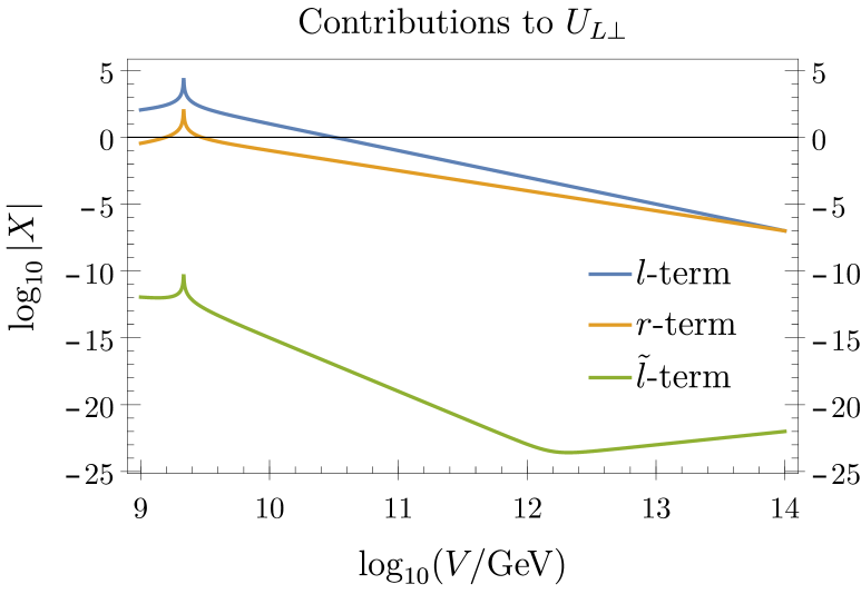
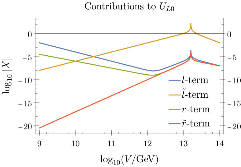
Figure 3: Comparison of the size of contributions to $U_{L\perp}$ from Eq. (3.35) (left panel) and to $U_{L0}$ from Eq. (3.36) (right panel). Each contribution is proportional to one of the coefficients $c\in\{l,r,\tilde{l},\tilde{r}\}$. If $c\neq 1$, a contribution shifts by $\log_{10}|c|$; for $|c|<1$ the shift is downward.

We plot the various contributions in the mixings $U_{L\perp}$ and $U_{L0}$ from Eqs. (3.35)–(3.36) as a function of the PS-scale $V$ in Fig. 3. Note that the plot shows contributions assuming the parameter values $\{l,r,\tilde{l},\tilde{r}\}$ to be equal $1$, otherwise the associated curves are shifted by an appropriate amount, cf. caption of Fig. 3. We see that $U_{L\perp}$ depends on $l$ and $r$, while the $\tilde{l}$ effect can be neglected. For $U_{L0}$ the situation is more complex: at small $V$ the $l$-term is the most important, followed by the $r$-term; at large $V$, the $\tilde{l}$-term dominates, while the other contributions are comparable. We observe cusps representing poles in the mixing angle, again due to mass cross-over as in Fig. 2. The coefficients $l,r,\tilde{l},\tilde{r}$ need to be taken sufficiently small so that $U_{L\perp},U_{L0}\ll 1$, otherwise we are outside the regime of Eq. (3.26).

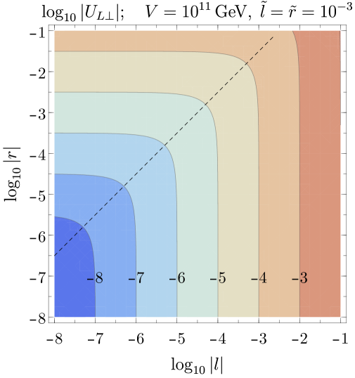
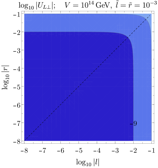
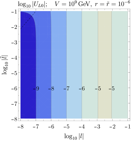
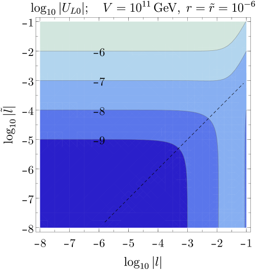
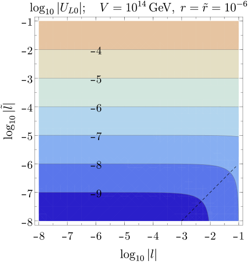
Figure 4: Contour plots for $\log_{10}$ of the size of mixing of L-neutrinos with anomalons. The upper row shows mixing with heavy anomalons $U_{L\perp}$ in the $l$-$r$ plane and benchmark values $\tilde{l}=\tilde{r}=10^{-3}$. The lower row shows mixing with light anomalons $U_{L0}$ in the $l$-$\tilde{l}$ plane and benchmark values $r=\tilde{r}=10^{-6}$. The columns represent three different values of the PS-breaking scale: $V=10^{9,11,14}\,\mathrm{GeV}$. The color coding is consistent for all plots, and the dashed lines represent where the contributions of the two terms from the $x$- and $y$-axis are equal, see main text.

We now have a good analytic understanding of the spectrum and mixing angles. The latter are rather involved, so it is useful to consider some benchmark scenarios. Contour plots of $\log_{10}|U_{L\perp}|$ and $\log_{10}|U_{L0}|$ for three different scales $V$ are shown in Fig. 4, where the former are drawn in the $l$-$r$ plane and the latter in the $l$-$\tilde{l}$ plane. More features are elaborated on in the points below:

• Since the situation for light mixing $U_{L0}$ is quite involved, we take small benchmark values for the remaining parameters $r$ and $\tilde{r}$ in order for their contributions not to interfere at any scale $V$.

• Numerical diagonalization of (3.24) rather than analytic formulae from Eqs. (3.35)–(3.36) was used for the plots. Consequently there is no upper bound on parameters limiting applicability, i.e. the right panel of Fig. 2 does not apply. Note, however, that in such regions the spectrum may be modified relative to Eq. (3.26) and non-linear features in the angles appear, specifically the inflection around $|l|\sim 10^{-2.5}$ in the bottom-left panel.

• The parameters associated to the two axes in each panel were taken with opposite signs. The region where their contributions to the mixing angle become equal are visually shown with a dashed line. If same-sign parameters were taken, the two contributions can be canceled along the dashed line, as can be seen also analytically from Eqs. (3.35)–(3.36), and thus the mixing angle is suppressed relative to the values in the plot.

We conclude the analysis of mixing angles by saying that we cross-checked the consistency of both the analytic expressions in Eqs. (3.35)–(3.36) as well as numeric behavior of Eq. (3.24) with the numeric behavior of the full $30\times 30$ neutrino-anomalon mass matrix of Eqs. (3.10)–(3.16). The spectrum and mixing angles from the full matrix indeed show analogous behavior, with some further subtleties:

1. There are $3$ active neutrinos, $16$ heavy- and $8$ light anomalons in the spectrum. Therefore there are more regions in parameter space of mass cross-over and thus enhancement of the mixing angle.

2. Whenever there is a sum of intermediate states in analytic expressions, the large number of states can easily cause an enhancement of one order of magnitude relative to the $4\times 4$ block case if most terms have the same sign.

3. Beside the cancellation of contributions to mixing angles from different blocks (the dashed lines in Fig. 4), cancellations can also happen between the many parameters in the same block. For example, contributions from the $L\Psi_{\perp}$ block to mixing with some specific heavy anomalon state are suppressed if tuning of the right combination of parameters $\mathcal{A}_{IN}$, $\mathcal{B}_{IN}$, and $\mathcal{B}^{\prime}_{IN}$ is performed.

3.3 How realistic is the Yukawa sector?

We now address the question whether the Yukawa sector is realistic, i.e., it should reproduce the masses, mixing angles and CP-violating phases of the SM (including the neutrino oscillation data). A full numeric fit is beyond the scope of this paper, but we shall argue by counting independent parameters.

The fermion mass matrices $M_{U}$, $M_{D}$ and $M_{E}$ of the up-, down-, and charged lepton sectors are given in Eqs. (3.7)–(3.9). For neutrinos, we consider a simplified case where no mixing with anomalons occurs, and we thus consider only the Dirac and Majorana type mass blocks $M_{LR}$ and $M_{RR}$ in Eq. (3.12) (and further expanded in Eqs. (3.19)) and (3.13), respectively. Crucially, all these expressions already have the gauge and family redundancies removed, cf. App. B.4, by making the choice in Eq. (3.6).

Given this choice of redundancy removal, the mass matrices referred to above depend on the following set of parameters and VEVs:

$$Y^{\Phi}_{1,2,3}, Y^{\Sigma}_{3}, Y^{\Sigma^{\prime}}_{2,3}, Y_{R},$$

$${\color[rgb]{0,0,1}v^{u\Phi}_{{\color[rgb]{0,0,0}1,2,3}}}, {\color[rgb]{0,0,1}v^{u\Sigma}_{{\color[rgb]{0,0,0}1,2,3}}}, {\color[rgb]{0,0,1}v^{u\Sigma^{\prime}}_{{\color[rgb]{0,0,0}1,2,3}}}, {\color[rgb]{0,0,1}v^{d\Phi}_{{\color[rgb]{0,0,0}1,2,3}}}, {\color[rgb]{0,0,1}v^{d\Sigma}_{{\color[rgb]{0,0,0}3}}}, {\color[rgb]{0,0,1}v^{d\Sigma^{\prime}}_{{\color[rgb]{0,0,0}2,3}}}, {\color[rgb]{1.0,0,0}Z}^{\ast}_{11,22,33,12,13,23},$$ (3.37)

where we explicitly listed the available values for the flavor or family index in the subscript. This amounts in total to $7$ Yukawa parameters, $15$ EW VEVs and $6$ PS-breaking VEVs. Note that EW VEVs are sourced by the SM Higgs VEVs, hence the normalization condition

$$\sum_{A}\left(|{\color[rgb]{0,0,1}v^{u\Phi}_{{\color[rgb]{0,0,0}A}}}|^{2}+|{\color[rgb]{0,0,1}v^{u\Sigma}_{{\color[rgb]{0,0,0}A}}}|^{2}+|{\color[rgb]{0,0,1}v^{u\Sigma^{\prime}}_{{\color[rgb]{0,0,0}A}}}|^{2}+|{\color[rgb]{0,0,1}v^{d\Phi}_{{\color[rgb]{0,0,0}A}}}|^{2}+|{\color[rgb]{0,0,1}v^{d\Sigma}_{{\color[rgb]{0,0,0}A}}}|^{2}+|{\color[rgb]{0,0,1}v^{d\Sigma^{\prime}}_{{\color[rgb]{0,0,0}A}}}|^{2}\right) =\tfrac{1}{2}\,v_{\rm EW}^{2},$$ (3.38)

where $v_{\rm EW}=246\,\mathrm{GeV}$. The EW VEVs depend on the admixture of the SM Higgs in every doublet component, which is determined from their mass matrix, which in turn depends on the parameters of the scalar potential of Eqs. (2.2)–(2.5). The structure of the scalar potential should be rich enough that the EW VEVs can be considered as independent.

The parameters in Eq. (3.37) are complex, with the exception of $Y^{\Sigma}_{3}$, $Y^{\Sigma^{\prime}}_{2}$, ${\color[rgb]{0,0,1}v^{d\Sigma}_{{\color[rgb]{0,0,0}3}}}$ and ${\color[rgb]{0,0,1}v^{d\Sigma^{\prime}}_{{\color[rgb]{0,0,0}2}}}$, which are made real as part of redundancy removal, see App. B.4 for details. With a large number of complex phases among the parameters, the fit of complex phases of the CKM and PMNS matrix are of least concern, and we thus focus on masses and mixing angles by use of real-valued parameters.

The real observables to be fit are $3$ masses each in the up-, down-, charge-lepton and neutrino sectors, $3$ CKM mixing angles and $3$ PMNS angles. This amounts to a total of $18$ values, which is less than the $7+15+6-1=27$ parameters of Eq. (3.37). Simple parameter counting thus suggests a fit should be possible.

Parameter counting arguments can fail if there are any flavor structure limitations arising from the mass matrices. We therefore make further refinements to our argument, by considering which sets of mass matrix entries are independent functions of the parameters listed in Eq. (3.37). The following observations are strongly indicative of no obstructions to a successful flavor fit:

1. The mass matrix of active neutrinos reduces in the limit of no mixing with anomalons to the standard seesaw expression:

   $$M_{\nu} =-M_{LR}M_{RR}^{-1}M_{LR}^{T}.$$ (3.39)

   Since $M_{RR}$ of Eq. (3.13) is an arbitrary (complex) symmetric matrix, since it depends on PS-breaking VEVs ${\color[rgb]{1.0,0,0}Z}^{\ast}_{AB}$ appearing nowhere else in the Yukawa sector, $M_{\nu}$ can also be set to be a symmetric complex matrix of choice independently from the $U$, $D$ and $E$ sectors. The neutrino masses and PMNS mixing angles are thus taken care of.

2. The remaining mass matrices $M_{U}$, $M_{D}$ and $M_{E}$ should thus fit the $9$ masses (of the $U$,$D$,$E$ sectors) and $3$ CKM mixing angles. The use of implicit function theorem reveals which entries in $M_{U,D,E}$ are independent and can be used for which observables; we shall argue based on counting results given in Table 3:

   • The number of independent diagonal entries in $M_{U,D,E}$ is $8$, namely $(M_{D})_{11}=(M_{E})_{11}$. This indicates $8$ of the $9$ masses can be fit independently by use of these entries, while the breaking of one relation requires involving off-diagonal entries.

   • In the LR convention and limit of small mixings, the left mixing angles dominantly arise from the strictly-upper-triangular entries of a matrix. Enlarging the set of diagonal entries by the upper-triangular part in $M_{U}$, we see that the $3$ new entries are independent from prior ones, enabling a description of the $3$ CKM angles.

   • Taking also the upper triangular parts of $M_{D}$ and $M_{E}$, we gain $3$ more mixings, providing the up-to-now missing parameter to separate all the masses, thus completing the list of SM observables in the Yukawa sector. The overhead of $2$ leftover independent parameters could even conceivably be used to help with the PMNS fit that we already established to be possible by using only the VEVs ${\color[rgb]{1.0,0,0}Z}^{\ast}_{AB}$ in the neutrino sector.

   • Including the lower triangular parts, the full matrices $M_{U,D,E}$ have in total $18$ independent parameters. This enlargement includes some right mixing angles that are unobservable in the SM.

set of entries	$\#$ independent
$\{\mbox{diag}\,M_{U},\mbox{diag}\,M_{D},\mbox{diag}\,M_{E}\}$	$8$
$\{\operatorname{upp}M_{U},\mbox{diag}\,M_{D},\mbox{diag}\,M_{E}\}$	$11$
$\{\operatorname{upp}M_{U},\operatorname{upp}M_{D},\operatorname{upp}M_{E}\}$	$14$
$\{M_{U},M_{D},M_{E}\}$	$18$

Table 3: The number $\#$ of independent entries with respect to the parameters of Eq. (3.37) in various subsets of mass-matrix entries from $M_{U,D,E}$ in Eqs. (3.7)–(3.9). The diagonal and upper-triangular part of a matrix are denoted by diag  and $\operatorname{upp}$, respectively.

We conclude that by all indications a fit of the SM masses, mixing angles and phases should be possible already in the case $N_{\Phi}=1$ and $N_{\Sigma}=2$, as has been alluded to in Sect. 3.1.

4 Phenomenological profile of the accidental/high-quality axion

In this section, we present a phenomenological overview of the accidental Pati-Salam axion, touching upon astrophysical axion limits, axion cosmology and direct searches. In summary, the key features closely resemble those of the benchmark DFSZ model [8, 9], albeit with significant constraints on the axion decay constant, which narrow down the allowed ranges for the axion mass: $m_{a}\in[2\times 10^{-8},10^{-3}]\,\mathrm{eV}$ (accidental ${\rm U}(1)_{\rm PQ}$, pre-inflationary PQ breaking scenario) and $m_{a}\gtrsim 0.01\,\mathrm{eV}$ (high-quality ${\rm U}(1)_{\rm PQ}$, post-inflationary PQ breaking scenario).

4.1 Astrophysical constraints

The goal of this section is to provide a lower bound on the axion decay constant, stemming from astrophysical limits on the axion couplings (for reviews on axion astrophysics, see e.g. [54, 55, 56]). The main constraints within our model arise from the axion couplings to electrons and nucleons. The latter can be expressed in terms of the axion-quark couplings provided in Eq. (2.25) (see e.g. [57, 58]), obtaining

$$c_{p} =-0.45\phantom{0}+0.29\cos^{2}\beta-0.15\sin^{2}\beta\,,$$ (4.1)

$$c_{n} =+0.013-0.14\cos^{2}\beta+0.27\sin^{2}\beta\,.$$ (4.2)

Defining $g_{aX}=c_{X}m_{X}/f_{a}$, with $X=p,n,e$, we consider the stringent limits imposed by Supernova (SN) 1987A [59, 60], as well as by the observed evolution of red giants [61, 62] and white dwarfs [63, 64], yielding respectively $g_{an}^{2}+0.61g_{ap}^{2}+0.53g_{an}g_{ap}\lesssim 8.3\times 10^{-19}$ and $g_{ae}\lesssim 2\times 10^{-13}$. Combining these two limits, the lowest value for $f_{a}$ is obtained by saturating the lower bound on $\beta$ set by perturbativity (i.e. $\tan\beta=0.25$), for which we obtain $f_{a}\gtrsim 2\times 10^{8}\,\mathrm{GeV}$. We observe that, for $\tan\beta\lesssim 0.5$, this limit is basically constant and is dominated by the SN 1987A bound.

Given the structural uncertainties related to the SN bound (see e.g. [65]), it is worth to mention that for $\tan\beta=0.25$ the bound on the axion decay constant stemming from the (tree-level) axion-electron coupling is $f_{a}\gtrsim 5\times 10^{7}\,\mathrm{GeV}$. Note, however, that in the small $\tan\beta$ limit the axion-electron coupling (cf. Eq. (2.25)) receives large radiative corrections from the axion coupling to the top-quark [66, 67, 68, 69, 70, 71, 72]. Including the latter correction, one obtains $c_{e}\simeq\frac{1}{3}\sin^{2}\beta+r^{t}_{e}(m_{\rm BSM})\frac{1}{3}\cos^{2}\beta$, where $m_{\rm BSM}$ denotes the energy scale of the non-SM Higgs doublets. Assuming e.g. that the effective theory below $f_{a}$ is the SM, i.e. $m_{\rm BSM}=f_{a}\simeq 10^{8}\,\mathrm{GeV}$, one finds $r^{t}_{e}(m_{\rm BSM})\simeq 0.23$ (cf. Table B.4 in Ref. [72]), from which we obtain

$$f_{a}\gtrsim 2.3\times 10^{8}\,\mathrm{GeV}\,,$$ (4.3)

that is slightly stronger than the SN bound derived above. The lower limit in Eq. (4.3) plays an important role for the issue of PQ quality, as discussed in Sect. 2.3.

4.2 Axion cosmology

The cosmological evolution of the axion field and the associated cosmological observables crucially depend on the interplay between the inflationary scale and the PQ symmetry-breaking scale, with standard considerations applicable also to our model (for reviews on axion cosmology see e.g. [73, 74]).

If the PQ is broken after inflation or restored afterwards (post-inflationary PQ breaking scenario), one also has topological defects, i.e. cosmic strings and domain walls, that contribute to the axion dark matter relic density, on top of the usual misalignment mechanism [75, 76, 77]. In particular, the contribution from topological defects can be significant and difficult to assess (see e.g. [78, 79]), so that a robust prediction for the axion dark matter mass is not possible at the moment. In any case, one can derive a lower bound on the axion dark matter mass, $m_{a}\gtrsim 28\,\mu\text{eV}$ (equivalently $f_{a}\lesssim 2.0\times 10^{11}\,\mathrm{GeV}$) [80], from the requirement of not overshooting the dark matter relic density. Note, however, that the entire dark matter abundance can be reproduced also for $m_{a}\gg 28\,\mu\text{eV}$, either through the contribution of topological defects (see e.g. [78, 81]) or non-standard axion production mechanisms (see e.g. [82]).

Specifically for our model, from Eq. (2.22) it follows that $N_{\rm DW}\equiv 2N=12$, so the model has a domain wall problem in the post-inflationary PQ-breaking scenario. The Lazarides-Shafi solution [83, 84], in which the $\mathbb{Z}_{N_{\rm DW}}$ discrete symmetry connecting the $N_{\rm DW}$ degenerate minima of the axion potential is fully embedded in the center of a non-abelian symmetry group, applies neither to the present Pati-Salam model nor to the original ${\rm SO}(10)$ model of Ref. [1]. More precisely, denoting the generator of the $\mathbb{Z}_{N_{\rm DW}}$ symmetry as $r_{12}$ and that of the centers of the $G_{\rm PS}\times{\rm SU}(3)_{f_{R}}$ gauge symmetries as $r_{4}r_{2}r_{2}r_{3}$, it can be checked that there is no solution for the system of equations $r_{12}=r_{4}^{m}r_{3}^{n}r_{2}^{k}r_{2}^{l}$, for integer values of $m,n,k,l$, when applied to the field content in Table 1. Hence, to address the domain wall problem, one needs to invoke a small breaking of the ${\rm U}(1)_{\rm PQ}$ via Planck suppressed operators, which could remove the degeneracy among the vacua of the axion potential, effectively causing the domain walls to decay before they dominate the energy density of the universe [85]. While the latter scenario is consistent with the general approach discussed here, in terms of an approximate ${\rm U}(1)_{\rm PQ}$ symmetry, the parameter space for such a solution is somewhat limited [86]. The aforementioned aspects reflect the tension between cosmology and the PQ quality problem, associated with the post-inflationary PQ breaking scenario [87].

Conversely, if the PQ symmetry is broken before inflation and not restored afterwards (pre-inflationary PQ-breaking scenario), the axion dark matter relic density depends on the (random) initial misalignment angle and hence it cannot be predicted. Nonetheless, dark matter axions are allowed to have masses of at most $m_{a}\lesssim 1\,\mathrm{meV}$ (equivalently $f_{a}\gtrsim 5.7\times 10^{9}\,\mathrm{GeV}$), because quantum fluctuations during inflation would imply too large iso-curvature fluctuations [88].

4.3 Axion searches

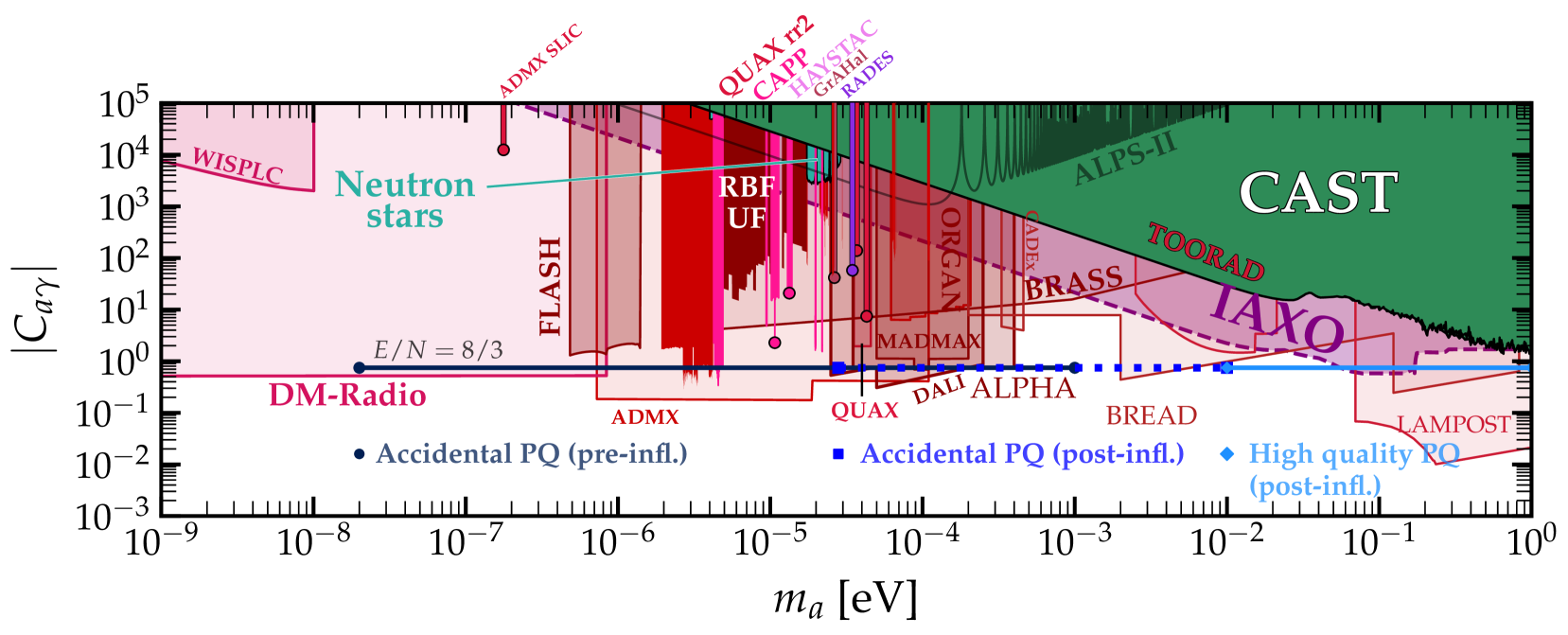
Figure 5: Axion-photon coupling (Eq. (A.20) with $E/N=8/3$) as a function of the axion mass. Current limits and future sensitivities are represented by filled and shaded regions, respectively. A high-quality PQ symmetry is obtained for $m_{a}\gtrsim 0.01\,\mathrm{eV}$ (light blue line) in the post-inflationary PQ-breaking scenario. An accidental PQ symmetry (not addressing the PQ-quality problem) corresponds to the intervals $m_{a}\in[2\times 10^{-8},10^{-3}]\,\mathrm{eV}$ in the pre-inflationary PQ-breaking scenario (black line) and $m_{a}\in[2.8\times 10^{-5},0.01]\,\mathrm{eV}$ in the post-inflationary PQ-breaking scenario (blue/dashed line). Axion limits adapted from [89].

Axion couplings to photons and SM matter fields have been computed in App. A (in Eq. (A.20) and Eqs. (A.26)–(A.27), respectively). For the present scenario, the axion coupling to photons (displayed in Fig. 5 as a function of the axion mass) represents the main experimental probe in the context of axion physics. The mass range of the accidental Pati-Salam axion is constrained by various considerations.

An absolute lower bound on $m_{a}$ is obtained within the model, since $f_{a}$ is bounded from above by the seesaw scale. From Eq. (2.24) we find the upper limit $f_{a}\leq V_{B-L}/12$, with $V_{B-L}\equiv\sqrt{V^{2}_{\chi}+4V^{2}_{\Delta}}$. Here, $V_{B-L}$ assumes the meaning of $B-L$ breaking scale, proportional to the mass of the $B-L$ gauge boson. This is subject to the constraints from the neutrino mass spectrum. In particular, the light neutrino masses are mainly controlled by $V_{\Delta}$ through the right-handed neutrino mass contributions, $M_{RR}\sim Y_{R}V_{\Delta}$. In contrast, $V_{\chi}$ has only a minor effect on the neutrino spectrum, as its contribution arises solely through the mixing with anomalons via non-renormalizable operators (cf. Sect. 3.2). Setting a robust upper limit on $V_{\Delta}$ would necessitate a fit to fermion masses and mixings, which goes beyond the scopes of the present work. However, barring fine-tuned regions in the global fit, one requires $V_{\Delta}\lesssim 10^{15}\,\mathrm{GeV}$ not to undershoot the active neutrino mass scale. Given this bound on $V_{\Delta}$, with $V_{\chi}$ unconstrained, the upper limit on $f_{a}$ is obtained in the $V_{\chi}\gg V_{\Delta}$ limit, corresponding to $f_{a}\approx V_{\Delta}/3$. Hence, we obtain $f_{a}\lesssim 3\times 10^{14}\,\mathrm{GeV}$ (equivalently $m_{a}\gtrsim 2\times 10^{-8}\,\mathrm{eV}$). Other constraints on the axion mass arise from cosmology, astrophysics and the requirement of PQ quality, as previously discussed and recalled in the caption of Fig. 5, which shows the prediction of the model (blue line) in the axion-photon vs. axion-mass plane, including also present constraints and future sensitivities [90, 91, 92, 93, 94, 95, 96, 97, 98, 99, 100, 101, 102, 103, 104, 105, 106, 107, 108, 109, 110, 111, 112, 113, 114, 115, 116, 117, 118, 119, 120]. In particular, we introduce two main scenarios for the allowed axion mass range in Fig. 5:

• High-quality PQ. This scenario, corresponding to a post-inflationary PQ breaking, is obtained for $m_{a}\gtrsim 0.01\,\mathrm{eV}$ (light blue line in the right side of Fig. 5). This setup is not directly testable at the moment, since axion experiments (both helioscopes and haloscopes) lose sensitivity in the $m_{a}\sim 0.01\,\mathrm{eV}$ ballpark, while for $m_{a}\gtrsim 0.025\,\mathrm{eV}$ astrophysical constraints prevent the full visibility of this parameter space. On the other hand, given the remnant $|\theta^{\rm min}_{\rm eff}|\simeq 4.7\times 10^{-13}$ in correspondence with astrophysical limits (cf. Sect. 2.3), an indirect way to test the high-quality PQ scenario is provided by the search for nucleon EDMs, which will improve the current sensitivity on $\theta_{\rm eff}$ by up to three orders of magnitude [49, 50, 51].

• Accidental PQ. This scenario, characterized by an accidental PQ symmetry that does not resolve the PQ-quality problem, can occur in either the pre- or post-inflationary PQ-breaking regime (in the latter case only for $m_{a}\gtrsim 28\,\mu\text{eV}$ [80]). The two cases correspond respectively to the black line on the left side of Fig. 5 ($m_{a}\in[2\times 10^{-8},10^{-3}]\,\mathrm{eV}$) and to the blue/dashed line ($m_{a}\in[2.8\times 10^{-5},0.01]\,\mathrm{eV}$). Barring a hole in sensitivity around $m_{a}\sim 10^{-3}\,\mathrm{eV}$, the parameter space of the accidental Pati-Salam axion will be mostly explored in the coming decades, under the crucial assumption that the axion comprises the entirety of dark matter.

5 Anomalon cosmology

The presence of parametrically light anomalons in the spectrum is a direct consequence of the gauging of the ${\rm SU}(3)_{f_{R}}$ flavor group. In this regard, the dynamics of anomalons represents a possible low-energy signature of the UV mechanism addressing the accidental origin of the PQ symmetry and the solution to the PQ quality problem. The mass spectrum of anomalons strongly depends on the PQ breaking scale $f_{a}$, or equivalently on the scale $V=3\sqrt{5}f_{a}$ (cf. Eq. (2.24)), as shown in the left panel of Fig. 2. The main result of Sect. 3.2 is that anomalons split into two sets: 16 heavy anomalons with mass $m_{\perp}$ and 8 light anomalons with mass $m_{0}$. The mass spectrum directly determines the cosmological history of the anomalon sector. We discuss this in two particular scenarios, following the classification introduced in Sect. 4.3:

• High-quality PQ. The PQ scale lies in the interval $f_{a}\in[2.3,5.6]\times 10^{8}\,\mathrm{GeV}$, corresponding roughly to $V\sim 10^{9}\,\mathrm{GeV}$. There are $N_{\Psi}=24$ ultra-light anomalons with masses below $0.1\,\mathrm{eV}$, as we observe from Fig. 2 (the distinction between heavy and light anomalons here is mostly irrelevant). The PQ symmetry is broken after the end of inflation, $T_{\rm RH}>f_{a}$.

• Accidental PQ. The PQ scale lies in the interval $f_{a}\in[5.7\times 10^{9},3\times 10^{14}]\,\mathrm{GeV}$, corresponding to $V\in[4\times 10^{10},2\times 10^{15}]\,\mathrm{GeV}$. The reheating temperature could satisfy either $T_{\rm RH}<f_{a}$ (pre-inflationary) or $T_{\rm RH}>f_{a}$ (post-inflationary). We discuss the following two benchmark sub-cases, referring to the results shown in Fig. 2:

  • for $V=10^{14}\,\mathrm{GeV}$ ($f_{a}\sim 10^{13}\,\mathrm{GeV}$), we have $m_{\perp}\sim 10$ TeV and $m_{0}\sim\mathrm{keV}$;

  • for $V=10^{11}\,\mathrm{GeV}$ ($f_{a}\sim 10^{10}\,\mathrm{GeV}$), we have $m_{\perp}\sim 10\,\mathrm{keV}$ and $m_{0}\sim\mu\mathrm{eV}$.

Following standard notation in cosmology, we define $T$ as the temperature of the photon thermal bath (or more generically the SM thermal bath for $T\gtrsim\mathrm{MeV}$, prior to neutrino decoupling). We introduce the Hubble expansion rate, $H(T)$, and the entropy density of the universe $s(T)$ as

$$H(T)=\sqrt{\frac{4\pi^{3}g_{*}(T)}{45}}\frac{T^{2}}{M_{\rm Pl}}\,,\qquad s(T)=\frac{2\pi^{2}}{45}g_{s}(T)T^{3}\,,$$ (5.1)

with the expression for the Hubble rate holding in a radiation-dominated universe. The functions $g_{s}(T)$ and $g_{*}(T)$ count the number of relativistic degrees of freedom (DOF) in the thermal bath and only differ at temperatures below $\sim 0.5\,\mathrm{MeV}$. For instance, at temperatures above EW symmetry breaking (EWSB) the number of SM DOF is $g_{*}^{\rm SM}=g_{s}^{\rm SM}\equiv g_{\rm SM}=106.75$, while for $T\ll 0.5\,\mathrm{MeV}$, $g_{s}^{\rm SM}=43/11\simeq 3.91$ and $g_{*}^{\rm SM}\simeq 3.36$. Extra particles (the axion, the anomalons, etc.) also contribute as long they are relativistic. Finally, the equilibrium interaction rate density for a 2-to-2 fermion annihilation $\overline{F}F\to\overline{\psi}\psi$ is defined as

$$\gamma_{{\rm eq}}(\overline{F}F\to\overline{\psi}\psi)=g_{F}^{2}\frac{T}{32\pi^{4}}\int_{4m_{F}^{2}}^{\infty}ds\,s^{3/2}\,\sigma_{\overline{F}F\to\overline{\psi}\psi}(s)\left(1-\frac{4m_{F}^{2}}{s}\right)K_{1}(\sqrt{s}/T)\,,$$ (5.2)

where $\sqrt{s}$ is the center-of-mass (c.o.m.) energy, $K_{1}$ is a Bessel function, $g_{F}$ is the number of polarization DOF of the initial states ($g_{F}=2$ for a Weyl fermion), and $\sigma(s)$ is the cross section of the process. The corresponding (equilibrium) interaction rate $\Gamma_{\rm eq}$ is defined in terms of the equilibrium number density of the Weyl fermions $n_{F,\rm eq}$ as

$$\Gamma_{\rm eq}=\frac{\gamma_{\rm eq}}{n_{F,\rm eq}}\,,\qquad n_{F,\rm eq}\simeq\frac{3\,g_{F}\,\zeta(3)}{4\pi^{2}}T^{3}\text{\ \ for \ \ }T\gg m_{F}\,.$$ (5.3)

The rest of this section is organized as follows: we present a general discussion on the production of anomalons in the early universe and their cosmological evolution in Sect. 5.1, and then discuss the phenomenology of anomalons as a component of dark radiation or dark matter in Sects. 5.2 and 5.3, respectively.

5.1 Anomalon production in the early universe

Anomalons communicate to the SM sector in different ways: $i)$ via the exchange of massive ${\rm SU}(3)_{f_{R}}$ flavor gauge bosons $W_{f_{R}}$, which interact at the renormalizable level with both anomalons and SM right-handed fermions, $ii)$ through neutrino-anomalon mixings induced by the the non-renormalizable operators of Table 2 (cf. discussion in section 3.2), which lead to neutrino-anomalon conversions, $iii)$ through effective Yukawa interactions, induced again by the non-renormalizable operators of Table 2. We define the total anomalon-SM interaction rate as $\Gamma_{\Psi}=\Gamma_{\Psi}^{\rm flavor}+\Gamma_{\Psi}^{\nu-\rm mix}+\Gamma_{\Psi}^{\rm Yuk}$. Anomalons are kept in thermal equilibrium with the SM bath whenever $\Gamma_{\Psi}(T)\gtrsim H(T)$. If this occurs, equilibrium is maintained until decoupling (or freeze-out) when $\Gamma_{\Psi}(T_{\rm dec})\simeq H(T_{\rm dec})$.

On the other hand, if the interactions are sufficiently weak such that $\Gamma_{\Psi}\ll H$ holds at any time of cosmological evolution, anomalons never reach thermal equilibrium. Assuming a vanishing anomalon abundance just after the end of inflation, a non-thermal population is then produced from scatterings (i.e. multiple scattering processes) of SM particles in the thermal bath, which occasionally produce anomalons as final states. This mechanism is generically referred to as freeze-in in the dark matter literature (see e.g. [121]).

As we will motivate extensively in the following, we are particularly interested in this second possibility (freeze-in). In such a case, the following independent populations of anomalons are produced:

1. First, via flavor gauge interactions, namely fermion annihilations $\overline{F}^{A}F^{B}\to(W_{f_{R}})\to\overline{\Psi}_{K}^{C}\Psi_{K}^{D}$, where $F$ are right-handed SM fermions and the intermediate step represents the $s$-channel exchange of a virtual flavor gauge boson. The anomalons are produced in the flavor basis: $A,B,C,D$ are ${\rm SU}(3)_{f_{R}}$ gauge indices and $K$ denotes the anomalon family, cf. Sect. 3.2, while all $W_{f_{R}}$ indices are left implicit.

2. A second population is produced via neutrino mixing, for instance processes such as $e^{+}e^{-}\to\overline{\nu}_{f}\nu_{f}\to\overline{\nu}_{f}\Psi_{m}$, where $\nu_{f}$ is a left-handed neutrino in the flavor basis ($f=e,\mu,\tau$), $\Psi_{m}$ an anomalon in the mass basis ($m=1,\dots,24)$ and the last step involves a neutrino-anomalon mixing angle $\theta_{\nu_{f}\Psi_{m}}$. This production mechanism is active only after EWSB (the mixing angles vanish before) and above $T\sim\,\mathrm{MeV}$ (neutrino decoupling). Notice that we use a slightly different and more compact notation compared to Sect. 3.2: $(\nu_{L})_{I}$ is replaced by $\nu_{f}$, while we denote the mixing between a flavor eigenstate $\nu_{f}$ and a mass eigenstate $\Psi_{m}$ as $\theta_{\nu_{f}\Psi_{m}}$.

3. A third population is produced through effective Yukawa interactions generated via the non-renormalizable operators of Table 2 (also responsible for the anomalon-neutrino mixings discussed above). These include effective $\overline{\nu}_{L}\Psi_{R}h$ and $\Psi_{R}\Psi_{R}h$ interactions ($h$ being the SM Higgs boson), as well as interactions of anomalons with heavy-scalar radial modes. Thus, anomalons are produced through decays of heavy-scalar radial modes, Planck-suppressed scalar annihilations and 2-to-2 annihilation of SM particles mediated by the Higgs boson.

5.1.1 Production via flavor interactions

We provide simple estimates for the interaction rate of flavor-mediated annihilations and the corresponding anomalon population. The ${\rm SU}(3)_{f_{R}}$ gauge bosons are massless at temperatures above the flavor breaking scale $T>V$. At lower temperatures they acquire a mass, which scales as $m_{W_{f_{R}}}\sim g_{f_{R}}V<V$, in terms of the flavor gauge coupling $g_{f_{R}}$ (we assume $g_{f_{R}}<1$). The production cross section scales as (up to $\mathcal{O}(1)$ factors and phase space)

$$\sigma_{\overline{F}F\to\overline{\Psi}\Psi}(s)\propto g_{f_{R}}^{4}\times\begin{cases}1/s\hskip 2.84544pt&\quad\text{ if }T>V\\ s/\left((s-m_{W_{f_{R}}}^{2})^{2}+m_{W_{f_{R}}}^{2}\Gamma_{W_{f_{R}}}^{2}\right)\hskip 2.84544pt&\quad\text{ if }T\leq V\\ \end{cases}\,,$$ (5.4)

with $\Gamma_{W_{f_{R}}}\propto g_{f_{R}}^{2}m_{W_{f_{R}}}\ll m_{W_{f_{R}}}$ being the decay width of $W_{f_{R}}$, while $F\in\{u_{R},d_{R},\nu_{R},e_{R}\}$ generically denotes the right-handed fermions (with flavor indices left implicit). In the lower case of Eq. (5.4), we recognize the Breit-Wigner formula, so that the cross-section gets a resonant enhancement when the c.o.m. energy of the process is $\sqrt{s}=m_{W_{f_{R}}}$.

In all the parameter space of our interest, $m_{\Psi}\ll m_{W_{f_{R}}}$ holds, and thus anomalons can be treated as effectively massless. We first focus on those annihilation channels which satisfy $m_{W_{f_{R}}}\gg m_{F}$. Far from the resonant region, the interaction rate can be estimated as

$$\frac{\Gamma_{\Psi}^{\rm flavor}}{H}\sim\frac{M_{\rm Pl}}{g_{*}^{1/2}T}\times\begin{cases}(g_{f_{R}}^{2}/4\pi)^{2}&\text{if }T\gg m_{W_{f_{R}}}\\ (T/V)^{4}&\text{if }T\ll m_{W_{f_{R}}}\end{cases}\,.$$ (5.5)

In the resonant peak we can adopt the small-width approximation, so that the cross section is $\sigma(s\sim m_{W_{f_{R}}}^{2})\sim g_{f_{R}}^{4}\pi s\,\delta(s-m_{W_{f_{R}}}^{2})/({m_{W_{f_{R}}}\Gamma_{W_{f_{R}}}})$ (see also [122]). The resonant peak corresponds to $T\simeq m_{W_{f_{R}}}$, and the interaction rate is enhanced as

$$\frac{\Gamma_{\Psi}^{\rm flavor}}{H}\bigg{|}_{\rm peak}\equiv\frac{\Gamma_{\Psi}^{\rm flavor}}{H}({T\simeq m_{W_{f_{R}}}})\sim\sqrt{\frac{g^{2}_{f_{R}}}{g_{*}(m_{W_{f_{R}}})}}\frac{M_{\rm Pl}}{V}\,.$$ (5.6)

The same result can equivalently be derived by considering the direct decay of $W_{f_{R}}$ to anomalons, along with its inverse processes. Flavor interactions are weak enough to avoid anomalon thermalization if $(\Gamma_{\Psi}^{\rm flavor}/H)|_{\rm peak}\ll 1$, which requires very small values for the flavor gauge coupling

$$g_{f_{R}}\ll 10^{-9}\left(\frac{V}{10^{9}\,\mathrm{GeV}}\right)\left(\frac{g_{*}(m_{W_{f_{R}}})}{106.75}\right)^{1/2}\,.$$ (5.7)

In such a scenario, the flavor gauge bosons can be quite light ($\lesssim\mathcal{O}(\mathrm{GeV})$ for $V=10^{9}\,\mathrm{GeV}$), but very weakly coupled to SM matter (the lighter, the less coupled). As long as $g_{f_{R}}\gtrsim 10^{-12}(10^{9}\,\mathrm{GeV}/V)$, there is always at least one resonant channel (electron-positron scattering).

Such small values of the gauge coupling can be avoided if the reheating temperature $T_{\rm RH}$ is low enough. Indeed, if $T_{\rm RH}\ll m_{W_{f_{R}}}$, the resonant enhancement is avoided, the cross-section always scales as $s/m_{W_{f_{R}}}^{4}$, and the production is maximal at $T=T_{\rm RH}$. Using the estimate in Eq. (5.5), anomalon thermalization is avoided even for an $\mathcal{O}(1)$ gauge coupling as long as

$$T_{\rm RH}\ll V\left(\frac{g_{*}^{1/2}(T_{\rm RH})V}{M_{\rm Pl}}\right)^{1/3}\simeq 10^{6}\,\mathrm{GeV}\left(\frac{V}{10^{9}\,\mathrm{GeV}}\right)^{4/3}\left(\frac{{g_{*}(T_{\rm RH})}}{106.75}\right)^{1/6}\,.$$ (5.8)

The allowed values of the reheating temperatures belong to the range $4\,\mathrm{MeV}\leq T_{\rm RH}\lesssim 10^{16}\,\mathrm{GeV}$ [43, 123, 124, 125]. However, Eq. (5.8) is only compatible with the pre-inflationary scenario, and can thus only be realized in the accidental PQ scenario (II).

Finally, we comment on those annihilation channels satisfying $m_{F}\gg m_{W_{f_{R}}}$, or equivalently $g_{f_{R}}\ll m_{F}/V$, which are thus not resonantly enhanced. Notice that this condition is satisfied for sterile neutrinos, as their mass is $m_{\nu_{R}}\equiv m_{R}\sim V$. If $m_{F}\ll T_{\rm RH}$, the cross section for anomalon production grows with decreasing temperature, and the production is maximal at $T\simeq m_{F}$. Non-thermalization implies the conservative constraint $g_{f_{R}}\ll(\sqrt{g_{*}}V/M_{\rm Pl})^{1/3}$, which is always weaker than the constraints from resonant annihilation channels and $W_{f_{R}}$ (inverse) decays. If $m_{F}\gg T_{\rm RH}$, the production channel is exponentially suppressed and irrelevant.

In summary, the anomalons never reach thermal equilibrium if either of the following conditions are met: Eq. (5.7), which allows for a large reheating temperature up to $T_{\rm RH}\lesssim 10^{16}\,\mathrm{GeV}$, or Eq. (5.8) with $g_{f_{R}}\lesssim\mathcal{O}(1)$. The freeze-in population of anomalons can be estimated in terms of the yield, $Y_{\Psi}\equiv n_{\Psi}/s$, as $Y_{\Psi}^{\rm flavor}\sim\gamma_{\rm eq}^{\rm flavor}/(Hs)$, giving

$$Y_{\Psi}^{\rm flavor}\sim\begin{cases}\frac{0.3\,g_{f_{R}}M_{\rm Pl}}{g_{s}^{3/2}V}\simeq 3\times 10^{-4}\,\left(\frac{g_{f_{R}}}{10^{-10}}\right)\left(\frac{10^{9}\,\mathrm{GeV}}{V}\right)\left(\frac{106.75}{g_{s}}\right)^{3/2}&{\text{if Eq.}~\eqref{eq:gcoupling}}\\ \frac{0.9M_{\rm Pl}T_{\rm RH}^{3}}{g_{s}^{3/2}V^{4}}\simeq 9.8\times 10^{-6}\left(\frac{T_{\rm RH}}{10^{5}\,\mathrm{GeV}}\right)^{3}\left(\frac{10^{9}\,\mathrm{GeV}}{V}\right)^{4}\left(\frac{106.75}{g_{s}}\right)^{3/2}&{\text{if Eq.}~\eqref{eq:TRH}}\\ \end{cases}\,,$$ (5.9)

where $g_{s}$ is computed at $T=\min\{m_{W_{f_{R}}},T_{\rm RH}\}$, and we assumed $g_{*}=g_{s}$ for simplicity.

As a final comment, we notice that fermion decays induced by flavor interactions, such as $F_{R}\to F^{\prime}_{R}\Psi_{R}\Psi_{R}$, are irrelevant. If $m_{F}\ll m_{W_{f_{R}}}$ the decay rate is suppressed as $\Gamma\propto m_{F}(m_{F}/V)^{4}$; if $m_{F}\gg m_{W_{f_{R}}}$, the rate is suppressed by the small gauge coupling $\Gamma\propto g_{f_{R}}^{4}m_{F}$. In both cases, the abundance of the decaying fermion is negligibly small at the time at which the decay should take place. Additionally, if $m_{F}\gg T_{\rm RH}$, the population of $F_{R}$ is exponentially suppressed.

5.1.2 Production via neutrino mixing

A second population of anomalons is produced via their mixing with the neutrino sector after EWSB. The relevant quantities are the mixing angles between the left-handed neutrino flavor eigenstates, $\nu_{f}$ ($f=e,\mu,\tau)$, and the anomalon mass eigenstates, $\Psi_{m}$ ($m=1,\ldots,24$), collectively denoted by $\theta_{\nu_{f}\Psi_{m}}$. These are induced by the non-renormalizable operators listed in Table 2 and have been discussed extensively in Sect. 3.2.2. We focus on the region of the parameter space where $\theta_{\nu_{f}\Psi_{m}}\ll 1$. More precisely, we require that the mixing angles are small enough to avoid anomalon thermalization from neutrino-anomalon conversions. If the anomalons are heavier than active neutrinos, $m_{\Psi_{m}}\gtrsim m_{\nu}$, this corresponds roughly to $\theta_{\nu_{f}\Psi_{m}}\lesssim[0.15-0.25]\,(0.1\,\text{eV}/m_{\Psi})^{1/2}$(as extrapolated from Refs. [126, 127, 128]). If instead $m_{\Psi_{m}}\lesssim m_{\nu}$, resonant effects are important and even smaller mixing angles are needed. Furthermore, bounds on dark radiation may even require stronger constraints on the mixing angles, as we discuss in more details below.

In Fig. 4 the mixings of L-neutrinos with massive anomalons are plotted as a function of the coefficients of the non-renormalizable operators of Table 2 (denoted by $U_{\perp}$ and $U_{0}$ for heavy and light anomalon mixings, respectively). As we can observe, for very large values of $V$ (accidental PQ scenario), small mixing angles can be achieved for both heavy and light anomalons without suppressing the coefficients of the operators. Conversely, in the high-quality PQ scenario, some of the coefficients need to be suppressed in order to avoid large mixings, in particular for the heavy anomalon sector ( the coefficients $\mathcal{A,B,B^{\prime},C}$ being the most relevant).

The physical picture is analogous to the production of $\mathrm{keV}$ sterile neutrino dark matter via oscillations (also referred to as Dodelson-Widrow mechanism) [129, 130, 131, 132, 133, 128, 126], in which active neutrino species produced in the thermal bath convert to $\mathrm{keV}$ sterile states via mixing. Applying this analogy, the $\mathrm{keV}$ sterile states correspond in our picture to massive anomalons.

There are, however, two important differences compared to the standard scenario. First, the anomalons may be lighter than active neutrinos. Moreover, most of the studies focus on the production of a single sterile state, while we must consider the simultaneous production of several anomalon species. A precise computation of the anomalon abundance would require the numerical solution of a set of quantum kinetic equations for neutrino-anomalon oscillations [127, 134, 128]. In the regime in which the anomalons are sufficiently heavy, $m_{\Psi}>m_{\nu}$, it is possible to derive approximate analytic estimates.

Let us first review the simple physical picture. As long as the temperature of the universe is $T\gtrsim\mathrm{MeV}$, active neutrinos are kept in thermal equilibrium with the photon bath through weak interactions, which produce neutrinos in the flavor basis, for instance from electron-positron annihilations, $e^{+}e^{-}\to\overline{\nu}_{f}\nu_{f}$, with rate $\Gamma_{\nu}\sim G_{F}^{2}T^{5}$, where $G_{F}\simeq 1.166\times 10^{-5}\,\mathrm{GeV}^{-2}$ is the Fermi constant. Some of the L-neutrinos convert to massive anomalons via mixing. The production rate $\Gamma_{m}$ for an anomalon mass eigenstate $\Psi_{m}$ depends on the (zero-temperature and zero-density) mixing angle $\theta_{\nu\Psi_{m}}^{2}\equiv\sum_{f=e,\mu,\tau}|\theta_{\nu_{f}\Psi_{m}}|^{2}$, where the proper sum over neutrino flavors is performed. These mixing angles receive corrections by thermal and density effects when neutrinos propagate in a thermal plasma [129, 130, 135]. We denote the finite temperature (and density) corrected angles by $\overline{\theta}_{\nu\Psi_{m}}$. The production rate scales then as $\Gamma_{m}\sim G_{F}^{2}T^{5}\overline{\theta}_{\nu\Psi_{m}}^{2}$. In the regime $m_{\Psi}\gg m_{\nu}$, one finds [136, 130]

$$\overline{\theta}_{\nu\Psi_{m}}\simeq\frac{\theta_{\nu\Psi_{m}}}{(1+\mathcal{O}(1)\frac{T^{6}G_{F}^{2}}{\alpha_{\rm em}m_{\Psi_{m}}^{2}})}\,.$$ (5.10)

The temperature at which the production is maximized depends on the anomalon mass eigenstate, $T_{\text{FI},m}\sim\max\,\{130\,\mathrm{MeV}(m_{\Psi_{m}}/\mathrm{keV})^{1/3},\mathrm{MeV}\}$. The resulting population can be estimated as $Y_{\Psi}^{\nu-{\rm mix}}\sim\gamma_{\rm eq}^{\nu-{\rm mix}}/(sH)\sim\sum_{m}(Y_{e,\rm eq}\Gamma_{m}/H)|_{T=T_{\text{FI},m}}$, where $Y_{\rm eq}$ is the equilibrium distribution for electrons/positrons. We find

$$Y_{\Psi}^{\nu-{\rm mix}}\big{|}_{m_{\Psi}\gg m_{\nu}}\sim{2.5\times 10^{4}}\left(\frac{10.75}{g_{\rm SM}}\right)^{3/2}\sum_{m=1}^{N_{\Psi}}\left(|\theta_{\nu\Psi_{m}}|^{2}\,\frac{m_{\Psi_{m}}}{\text{keV}}\,\right)\,.$$ (5.11)

The picture changes significantly if $m_{\Psi}\lesssim m_{\nu}$, which is the most typical situation we expect to be realized in the post-inflationary scenario. In such a case, the anomalon-neutrino conversion rate gets a resonant enhancement due to the presence of a pole in $\overline{\theta}_{\nu\Psi_{m}}$ [127]. This arises whenever the neutrino propagating in the thermal plasma acquires a momentum $p^{2}\sim\alpha_{\rm em}(m_{\nu}^{2}-m_{\Psi}^{2})/(G_{F}^{2}T^{4})$. Thus, the resonance propagates to higher momenta as the temperature decreases. This implies that the resonance eventually covers the full momentum distribution of neutrinos. As a result, resonant neutrino-anomalon conversions lead to very efficient thermalization of the anomalons if the mixing angle is not sufficiently small. To avoid this, the mixing angles $\theta_{\nu_{f}\Psi_{m}}$ must be significantly smaller compared to the non-resonant case. The precise condition as well as an accurate computation of the anomalons abundance in this regime is rather involved and requires a numerical solution of the quantum kinetic equations [127, 134, 128], with no simple analytic expression available. A full numerical computation is also very challenging and therefore many studies focus on the production of only one sterile state (often making simplifying assumption on the flavor mixings among active states). A complete computation within our framework lies beyond the scope of this study and is deferred to future work.

5.1.3 Production from effective Yukawa interactions

The non-renormalizable operators of Table 2 provide an extra production source for anomalons, namely through effective Yukawa interactions with the scalar fields of the model. We distinguish two classes of operators: those involving EW-breaking scalar fields $\Phi,\Sigma,\Sigma^{\prime}$ which after EWSB generate interactions with the SM Higgs boson $h$, and those involving only the heavy scalar fields $\Delta$ and $\chi$. We begin our discussion by considering the first class. The operator $\mathcal{A}\,\overline{Q}_{L}\Psi_{R}\chi\Phi/M_{\rm Pl}$ generates the effective Yukawa coupling $\mathcal{A}(V/M_{\rm Pl})\,\overline{\nu}_{L}\Psi_{R}h$ at scales below the EWSB. The same applies to the operators $\mathcal{B}\,\overline{Q}_{L}\Psi_{R}\chi\Sigma/M_{\rm Pl}$ and $\mathcal{B}^{\prime}\,\overline{Q}_{L}\Psi_{R}\chi\Sigma^{\prime}/M_{\rm Pl}$. Concurrently, the operators $\tilde{\mathcal{D}}\,\Psi_{R}\Psi_{R}\Phi^{*2}/M_{\rm Pl}$ (and analogously, the $\mathcal{E}$-type operators) generate the Yukawa interaction $(v/M_{\rm Pl})\,\Psi_{R}\Psi_{R}h$ as well as $\Psi_{R}\Psi_{R}h^{2}/M_{\rm Pl}$.

The $\Psi_{R}\Psi_{R}h$ and $\Psi_{R}\Psi_{R}h^{2}$ interactions are irrelevant in view of the extreme suppression factor $v/M_{\rm Pl}\sim 10^{-17}$. On the other hand, the $\overline{\nu}_{L}\Psi_{R}h$ coupling gives rise to Higgs decays $h\to\nu\Psi$ as well as $s$-channel Higgs-boson-mediated annihilations $PP\to(h)\to\nu\Psi$, where $PP\in\{\overline{F}F,W^{+}W^{-},ZZ,hh\}$ are the SM particles interacting with the Higgs boson. We checked that $(i)$ these new channels are unable to produce a population of anomalons in thermal equilibrium with the SM bath as long as $\mathcal{A,B,B^{\prime}}\ll 10^{-8}(M_{\rm Pl}/V)\simeq 10^{-3}(10^{14}\,\mathrm{GeV}/V)$, which is satisfied even for $\mathcal{A,B,B^{\prime}}\sim\mathcal{O}(1)$ as long as $V\lesssim 10^{11}\,\mathrm{GeV}$, and $(ii)$, the corresponding population of anomalons produced by freeze-in is typically small in most of the parameter space, so we neglect it. Notice that the branching ratio of the Higgs boson into $\nu\Psi$ is so small that there are basically no relevant constraints from Higgs invisible decays [137].

The second class of operators only involves heavy scalar fields. The most relevant ones are $\mathcal{C}\,Q_{R}\Psi_{R}\Delta^{*}\chi/M_{\rm Pl}$ and $\mathcal{D}\,\Psi_{R}\Psi_{R}\Delta^{*}\chi^{2}/M_{\rm Pl}^{2}$. These induce the decays of radial modes of $\Delta$ and $\chi$ to $\Psi_{R}\nu_{R}$ or $\Psi_{R}\Psi_{R}$(+ heavy scalar mode). Their rates are suppressed at least by a factor $(V/M_{\rm Pl})^{2}$, so that the decays are completely irrelevant (they would occur at $T\ll V$, when the heavy scalars have already disappeared from the thermal bath). Annihilations mediated by heavy scalars give weaker constraints compared to the ones mediated by the Higgs boson.

Finally, all the operators discussed in this section induce annihilations of scalar particles at large temperature. The most relevant ones are the operators of dimension 5, which induce processes such as $\chi\Phi\to Q_{L}\Psi_{R}$ or $\Phi\Phi\to\Psi_{R}\Psi_{R}$ or $\Delta\chi\to Q_{R}\Psi_{R}$. The corresponding population of anomalons is controlled by the reheating temperature, $Y\propto\mathcal{X}^{2}(T_{\rm RH}/M_{\rm Pl})$ with $\mathcal{X}\in\{\mathcal{A,B,B^{\prime},C,\tilde{D},E}\}$.

5.1.4 Anomalon decay

The decay modes of the anomalons and their rates crucially depend on their mass. We can anticipate the general result of this section referring to Fig. 2 and our different scenarios: the heavy anomalons of mass $m_{\perp}\sim 10$ TeV decay in the early universe, well before the onset of BBN. The ultra-light anomalons with mass $m\lesssim$ 0.1 eV are stable on cosmological scales. The $\mathrm{keV}$-ish anomalons are cosmologically stable for relatively small mixings. Stronger constrains on the mixings are provided by X-ray searches.

We now briefly discuss each one of these cases. Anomalons heavier than the TeV scale can decay through (some of) the operators of Table 2 involving EW-breaking fields. For instance, the dimension-5 operator $\mathcal{A}\,\overline{Q}_{L}\Psi_{R}\Phi\chi$ allows for $\Psi_{R}\to\Phi\mathcal{Q}_{L}$ (before EWSB), or analogously $\Psi_{R}\to h\nu_{L}$ (after EWSB). Additionally, extra decay channels are open, such as $\Psi_{R}\to\nu\overline{f}f$ after EWSB, which are mediated by a tree-level exchange of a Higgs boson or an EW gauge boson. These decays are fast enough to safely avoid cosmological constraints.

Anomalons with mass in the $1\div 100\,\mathrm{keV}$ range dominantly decay via neutrino mixing to $3\nu_{L}$, with decay width

$$\Gamma_{3\nu}=\frac{G_{F}^{2}m_{\Psi}^{5}\theta_{\nu\Psi}^{2}}{96\pi^{3}}\,.$$ (5.12)

They are cosmologically stable if $\theta_{\nu\Psi}\lesssim 0.018(10\,\mathrm{keV}/m_{\Psi})^{5/2}$. The decay channel $\Psi_{R}\to\nu_{L}\gamma$ is also open with rate

$$\Gamma_{\nu\gamma}=\frac{9\alpha_{\rm em}G_{F}^{2}m_{\Psi}^{5}\theta_{\nu\Psi}^{2}}{256\pi^{4}}\,.$$ (5.13)

Although subdominant, the latter process actually imposes the strongest constraints on the mixing; X-ray searches exclude $\theta_{\nu\Psi}\gtrsim 2\times 10^{-6}(10\,\mathrm{keV}/m_{\Psi})^{5/2}$ (see [138]).

Ultra-light anomalons could decay via the same channels of $\mathrm{keV}$-ish ones if $m_{\Psi}>m_{\nu}$, but they are cosmologically stable, as their decays are suppressed by their small mass $\Gamma\propto(m_{\Psi}/v)^{4}$. The same also applies to the decays of active neutrinos into anomalons when $m_{\Psi}<m_{\nu}$.

Finally, notice that the decays of heavy anomalons to lighter ones are suppressed, as they involve the exchange of a flavor gauge boson. These decays are completely irrelevant in all scenarios: heavy anomalons $m_{\perp}\gtrsim$ TeV decay much faster via the other decay channels discussed above; ultra-light anomalons are still cosmologically stable; for $\mathrm{keV}$-ish anomalons we should compare these decays with Eq. (5.12). The exchange of a flavor gauge boson implies a decay rate, which is suppressed at least by $1/(G_{F}^{2}V^{4}\theta_{\nu\Psi}^{2})\sim(v/V)^{4}(1/\theta_{\nu\Psi})^{2}$ compared to the decay channel into $3\nu_{L}$. Thus, even in the most pessimistic case ($V\sim 10^{9}\,\mathrm{GeV}$), the decays to active neutrinos are dominant unless $\theta_{\nu\Psi}\lesssim 10^{-13}$.

5.2 Anomalons as dark radiation

We focus here on the case of ultra-light sub-$\mathrm{eV}$ anomalons, arising mainly in the post-inflationary scenario and possibly as a subset of states in the pre-inflationary one (see Fig. 2). Being fermions, such low masses prevent them from being suitable dark matter candidates in view of the Tremaine-Gunn bound [139]. More precisely, a recent study of dwarf spheroidal galaxies finds the model-independent lower bound $m_{\Psi}\gtrsim 0.1\,\mathrm{keV}$ on the mass of a fermionic dark matter species [140] (assuming 100% of dark matter is made by that fermion).

On the other hand, such light particles are relativistic at the time at which the Cosmic Microwave Background (CMB) forms, $T_{\rm CMB}\sim$ 0.1 eV, as well as at the onset of Big Bang Nucleosynthesis (BBN), $T_{\rm BBN}\sim 0.1\,\mathrm{MeV}$, thereby contributing to the energy density of the universe in the form of extra radiation (in addiction to photons and neutrinos), commonly referred to as dark radiation. This is parameterized in terms of an effective number of neutrinos as (see e.g. [141])

$$\Delta N_{\rm eff}=\frac{8}{7}\left(\frac{11}{4}\right)^{4/3}\frac{\rho_{\Psi}}{\rho_{\gamma}}\,,$$ (5.14)

where $\rho_{\Psi}$ and $\rho_{\gamma}$ are respectively the anomalon and photon energy densities ($\rho_{\gamma}=2\pi^{2}T^{4}/30$), both evaluated at $T\sim T_{\rm CMB}$ (or $T\sim T_{\rm BBN}$). The current upper bound on $\Delta N_{\rm eff}$ has been set by the Planck collaboration: $\Delta N_{\rm eff}\leq 0.285$ (at $95\%$ C.L.) [43]. Forthcoming experiments aim to improve this bound up to roughly one order of magnitude with more precise CMB data: the Simon Observatory (SO) claims a sensitivity of $\Delta N_{\rm eff}(2\sigma)\leq 0.06$ [142, 143], while EUCLID [144] and future generation experiments such as CMB-HD [145] are expected to measure values down to $\Delta N_{\rm eff}\leq 0.014$. See also Ref. [146] for a review on current constraints and future sensitivities.

The current upper bound is badly violated if the light anomalons were ever in thermal equilibrium with the SM bath and decoupled at some temperature $T_{\rm dec}$. Indeed, in such a case, their contribution to $\Delta N_{\rm eff}$ is

$$\Delta N_{\rm eff}^{\rm TH}=N_{\Psi}\left(\frac{11}{4}\frac{g_{s}(T_{\rm CMB})}{g_{s}(T_{\rm dec})}\right)^{4/3}\simeq 1.13\,\frac{N_{\Psi}}{24}\left(\frac{106.75}{g_{s}(T_{\rm dec})}\right)^{4/3}.$$ (5.15)

Hence, this scenario is excluded even if only 8 anomalons are ultra-light and decoupled before EWSB.

On the other hand, the picture changes completely if the anomalons never reach thermal equilibrium and are produced by freeze-in, as we discussed previously. The computation of $\Delta N_{\rm eff}$ for species not in thermal equilibrium is a non-trivial task, since it requires accounting for non-thermal distributions for dark radiation, which strongly depend on the specific production mechanism. See e.g. Ref. [147] which discusses the scenario where decays or 2-to-2 scatterings of bath particles produce one relativistic dark particle in the final state. A detailed computation is beyond the scope of this paper. To simplify the analysis, we briefly discuss two possible approaches sometimes adopted in the literature.

The first possibility is to assume that the anomalon number density, $n_{\Psi}$, and the corresponding energy density, $\rho_{\Psi}$, are related as $\rho_{\Psi}\propto n_{\Psi}^{4/3}$, i.e. the same as for species in thermal equilibrium. Eq. (5.15) can be generalized and expressed in terms of the anomalon yield, $Y_{\Psi}=n_{\Psi}/s$, as [148, 149, 150]

$$\Delta N_{\rm eff}^{\rm FI1}\simeq N_{\Psi}\left(\frac{\frac{11}{4}\frac{2\pi^{4}}{45\xi(3)}\frac{2g_{s}^{\rm SM}(T_{\rm CMB})Y_{\Psi}}{3N_{\Psi}}}{1-\frac{2\pi^{4}}{45\xi(3)}\frac{7}{6}Y_{\Psi}}\right)^{4/3}\simeq 76.28\,\frac{Y_{\Psi}^{4/3}}{N_{\Psi}^{1/3}}\,.$$ (5.16)

Alternatively, we can drop the assumption $\rho_{\Psi}\propto n_{\Psi}^{4/3}$ and estimate $\Delta N_{\rm eff}$ as follows: the freeze-in production of the anomalons is maximally efficient at some temperature $T_{\rm FI}$ (which depends on the specific production mechanism). Since anomalons are produced by scatterings of SM bath particles, each one carrying energy $E\sim T$, their average energy immediately after production is also of order $\sim T$. Therefore, we can parametrize their energy density as $\rho_{\Psi}(T_{\rm FI})\simeq\xi T_{\rm FI}n_{\Psi}(T_{\rm FI})=\xi T_{\rm FI}s(T_{\rm FI})Y_{\Psi}$, where $\xi$ is an $\mathcal{O}(1)$ number. The energy density of a relativistic particle redshifts as a function of the scale factor $a_{T}\equiv a(T)$ as $\rho_{\Psi}(T)=\rho_{\Psi}(T_{\rm FI})(a_{T_{\rm FI}}/a_{T})^{4}=\rho_{\Psi}(T_{\rm FI})(T/T_{\rm FI})^{4}(g_{s}(T)/g_{s}(T_{\rm FI}))^{4/3}$. At the time of the CMB, this corresponds to

$$\Delta N_{\rm eff}^{\rm FI2}\simeq\frac{16}{21}\left(\frac{11}{4}\right)^{4/3}\frac{g_{s}(T_{\rm CMB})^{4/3}}{g_{s}(T_{\rm FI})^{1/3}}\xi Y_{\Psi}\simeq 56.96\left(\frac{\xi}{3.151}\right)\frac{Y_{\Psi}}{g_{s}(T_{\rm FI})^{1/3}}\,,$$ (5.17)

where in equilibrium $\rho_{\Psi}^{\rm eq}/n_{\Psi}^{\rm eq}=3.151\,T$ for a fermionic species. This expression is the equivalent of the one derived in Appendix C of [150], for the case of one spin-0 particle (the axion), generalized to our case with $N_{\Psi}$ Weyl fermions contributing to $\Delta N_{\rm eff}$. See also [151] for a numerical computation of $\Delta N_{\rm eff}$ in the freeze-in regime.

The expression in Eq. (5.17) relies on a more precise (though still approximate) estimate of the anomalon energy density, while Eq. (5.16) is an excellent approximation only when the anomalons follow their equilibrium distribution. Therefore, we will employ Eq. (5.17) for our estimates. More precisely, Eq. (5.16) underestimates the contribution to dark radiation by a factor $\Delta N_{\rm eff}^{\rm FI1}/\Delta N_{\rm eff}^{\rm FI2}\simeq 0.23\,(g_{s}(T_{\rm FI})/10.75)^{4/9}(\Delta N_{\rm eff}^{\rm FI2}/0.285)^{1/3}$.

We can now estimate the anomalon contribution to $\Delta N_{\rm eff}$ in our model, discussing separately the two scenarios introduced above.

5.2.1 High-quality PQ

The abundance of anomalons produced via renormalizable flavor interactions is given by the upper case of Eq. (5.9), requiring also $g_{f_{R}}\ll 10^{-9}$. The corresponding values of $\Delta N_{\rm eff}$ are generically below the experimental sensitivity of future experiments unless we saturate the freeze-in condition close to $g_{f_{R}}\sim 10^{-9}$, where our estimates are not reliable. Indeed, at the border between the freeze-in and thermalization regimes, a more precise computation of the abundance would be needed. As we know that thermalized anomalons are already excluded by the Planck ’18 result, we expect that, in order to interpolate between the two regimes, $\Delta N_{\rm eff}$ could reach values testable in the near future in that corner of the parameter space.

On the other hand, the production of anomalons via neutrino-anomalon conversion generically requires small mixing angles to satisfy the constraints on $\Delta N_{\rm eff}$. In the non-resonant scenario, $m_{\Psi}\gtrsim m_{\nu}$, the population of anomalons can be roughly estimated as in Eq. (5.11), which saturates the Planck ’18 bound for $\theta_{\nu\Psi_{m}}\simeq 0.014\,(0.1\,\mathrm{eV}/m_{\Psi_{m}})^{1/2}$ in a simplified scenario where all the anomalons have the same masses and mixing angles, or $\theta_{\nu\Psi_{1}}\simeq 0.066\,(0.1\,\mathrm{eV}/m_{\Psi_{1}})^{1/2}$ in the limit in which only one anomalon ($\Psi_{1}$) has a sizable mixing angle $\theta_{\nu\Psi_{1}}\gg\theta_{\nu\Psi_{j}}$. However, the typical expectation from the discussion of the spectrum in Sect. 3.2 is that anomalons are lighter than active neutrinos. In such a case, resonant effects enhance the production, inducing more severe constraints on the mixing angles. These imply a set of non-trivial constraints on the parameters of the model. In particular, the coefficients of the non-renormalizable operators of Table 2 need to be suppressed enough to avoid thermalization via resonant conversion. A detailed numerical analysis would be required in this case to accurately compute the anomalon abundance and its impact on restricting the model’s parameter space.

Finally, we note that for relatively low values of $f_{a}$ (as derived from the analysis of the PQ quality in Sect. 2.3, where $f_{a}\lesssim 5\times 10^{8}\,\mathrm{GeV}$), axions are efficiently produced at temperatures around or below the QCD phase transition through scattering of pions (see e.g. [152, 153, 154, 155, 156, 157]). Consequently, disentangling the axion contribution to $\Delta N_{\rm eff}$ from that of the anomalons is a non-trivial task, necessitating a comprehensive global analysis, which we defer to future work.

5.2.2 Accidental PQ

The results depend strongly on the scales $V$ and $T_{\rm RH}$. For large values of $V\sim 10^{14}\,\mathrm{GeV}$ (IIa), all the anomalons are heavier than $1\,\mathrm{keV}$ and either decay before BBN (cf. Sect. 5.1.4) or contribute to dark matter (cf. Sect. 5.3). For smaller values of $V\sim 10^{11}\,\mathrm{GeV}$ (IIb), 8 anomalons are ultra-light and contribute to dark radiation. Given that $f_{a}\sim 10^{10}\,\mathrm{GeV}$, anomalon thermalization via renormalizable flavor interactions is inefficient if either $T_{\rm RH}\lesssim V(V/M_{\rm Pl})^{1/3}\simeq 10^{8}\,\mathrm{GeV}$ (pre-inflationary) or $g_{f_{R}}\ll 10^{-7}$ (post-inflationary). Their abundance is given by the lower (upper) case of Eq. (5.9) in the first (second) scenario. The contribution to $\Delta N_{\rm eff}$ is again below current and future experimental sensitivities as long as Eq. (5.8) is satisfied. Once again, close to the thermalization regime, corresponding to $T_{\rm RH}\sim V(V/M_{\rm Pl})^{1/3}$ in the pre-inflationary scenario, we expect a larger and possibly testable value of $\Delta N_{\rm eff}$. Production from neutrino conversions is typically subdominant in light of the small mixing angles, see Fig. 4 (lower center). A detailed scan of the parameter space would be needed to provide more precise results.

5.3 Anomalons as dark matter

In the accidental PQ scenario, the model predicts a set of $\mathrm{keV}$-ish anomalons for some values of $V$, see Fig. 2. In some region of the parameter space, these can be cosmologically stable and not excluded by X-ray searches. Thus, they can contribute to the dark matter abundance of the universe, together with the axion. The physics is essentially the same as that of the well-studied $\mathrm{keV}$ sterile neutrino DM scenario, already briefly discussed in the previous section. While a detailed scan of the parameter space would be needed to provide precise results, we summarize here the main qualitative features.

For instance, if $V=10^{14}\,\mathrm{GeV}$ ($f_{a}\sim 10^{13}\,\mathrm{GeV}$), the 8 light anomalons have mass $m_{0}\sim 1\div 10\,\mathrm{keV}$. As long as $T_{\rm RH}\lesssim V(V/M_{\rm Pl})^{1/3}$ $\sim 10^{12}\,\mathrm{GeV}$ (pre-inflationary) or $g_{f_{R}}\ll 10^{-4}$ (post-inflationary), they are produced by freeze-in. The mixing with active neutrinos depends mostly on the parameters $\tilde{\mathcal{A}}$ and $\tilde{\mathcal{B}}$, as shown in Fig. 4 (lower right). Mixings larger than roughly $10^{-(6\div 5)}$ are already excluded by X-ray searches, while smaller angles are allowed. The population produced via mixing can still be the larger one even if mixings are small, $Y_{\rm light}^{\nu-{\rm mix}}\lesssim 10^{-8}(\theta_{\nu\Psi}/10^{-7})^{2}(m_{0}/10\,\mathrm{keV})$. This corresponds to a very small fraction of the total dark matter abundance, $\Omega_{\Psi,0}/\Omega_{\rm DM}\sim 10^{-3}$ (potentially up to 1% if we push $T_{\rm RH}$ up to $\sim 10^{12}\,\mathrm{GeV}$, where the computation is not fully reliable), which is not constrained by warm dark matter limits.

On the other hand, if $V=10^{11}\,\mathrm{GeV}$, the picture reverses, as the 16 heavy anomalons are now the $\mathrm{keV}$-ish ones, $m_{\perp}\sim 10\,\mathrm{keV}$. They possibly contribute to a small fraction of dark matter, analogous to the discussion above. The mixing angles are mostly determined by the coefficients $\mathcal{A},\mathcal{B},\mathcal{C}$, see Fig. 4 (upper center), and tend to be slightly larger than in the previous case, so that X-ray searches would impose more severe constraints on the model parameters.

6 Conclusions and outlook

In this study, we have investigated a category of axion models where the accidental ${\rm U}(1)_{\rm PQ}$ symmetry naturally arises from the interplay between vertical (grand-unified) and horizontal (flavor) gauge forces. Concentrating on a Pati-Salam implementation, which shares certain parallels with a prior SO(10) model examined in Ref. [1], we analyzed the model’s ability to address the PQ quality problem and we showed that it can non-trivially reproduce the SM flavor structure.

The main predictions of the model, regarding axion phenomenology, are summarized in Fig. 5, where three distinct axion mass windows are identified: $i)$ $m_{a}\in[2\times 10^{-8},10^{-3}]\,\mathrm{eV}$, $ii)$ $m_{a}\in[2.8\times 10^{-5},0.01]\,\mathrm{eV}$ (corresponding to an accidental ${\rm U}(1)_{\rm PQ}$, respectively in the pre-inflationary and post-inflationary PQ breaking scenario), and $iii)$ $m_{a}\gtrsim 0.01\,\mathrm{eV}$ (associated with a high-quality ${\rm U}(1)_{\rm PQ}$ in the post-inflationary PQ breaking scenario). In this context, the predictions of the Pati-Salam model regarding axion physics are largely degenerate with those of the original SO(10) model discussed in Ref. [1]. While the axion-photon coupling matches that of the benchmark DFSZ model [8, 9], the non-trivial embedding of the axion into the scalar multiplets of the extended gauge symmetry establishes a connection between the axion decay constant and intermediate mass scales associated with $B-L$ and flavor breaking.

A key feature of this setup is the presence of parametrically light fermions, known as anomalons, that were introduced to cancel the gauge anomalies of the flavor symmetry. For the most favorable PQ-breaking scales required to resolve the PQ quality problem, these anomalons are expected to have masses below the eV scale. As a result, they contribute to the dark radiation of the universe. While for intermediate-scale values of $f_{a}$, the anomalons can be heavier (keV scale) and thus contribute to dark matter.

We studied the cosmological production of anomalons in the early universe, considering their production via flavor interactions, neutrino mixing and effective Yukawa-like operators. Current constraints on the effective number of relativistic species, $\Delta N_{\rm eff}$, from Planck’18 [43] data were applied to constrain the parameter space. We further highlighted how future precision measurements of $\Delta N_{\rm eff}$ could serve as a low-energy probe of the UV dynamics underlying the solution to the PQ quality problem.

More generally, the cosmological signatures of the anomalon fields crucially depend on $f_{a}$. We present here a brief summary of our findings in two relevant benchmark scenarios:

• High-quality PQ (post-inflationary PQ-breaking scenario). All the anomalons contribute to dark radiation. In order to evade the current bound from the Planck ’18 analysis we must enforce the condition that they never reach thermal equilibrium (freeze-in), implying very small flavor gauge coupling $g_{f_{R}}\lesssim 10^{-9}$, as well as small mixings with active neutrinos. This imposes severe constraints on the parameter space of the model. The contribution to $\Delta N_{\rm eff}$ is below the sensitivity of future planned experimental proposals, with the exception of the region of the parameter space at the border between the thermalization and freeze-in regimes, where we expect a larger amount of dark radiation but a more precise computation would be needed.

• Accidental PQ (both pre-inflationary and post-inflationary PQ-breaking can be realized). The parameters of the model are less constrained and the phenomenology is richer. The mixings with active neutrinos are typically smaller compared to the scenario (I). This, and the defining condition $f_{a}>T_{\rm RH}$, more naturally forbid anomalon thermalization in the pre-inflationary scenario. In the post-inflationary scenario, a small flavor gauge coupling is needed (even though larger values than in the high-quality PQ scenario are admissible). We discussed two sub cases: (IIa) $f_{a}\sim 10^{13}\,\mathrm{GeV}$, where the 16 heavy anomalons have masses $m_{\perp}\sim 10\,\mathrm{TeV}$ and decay before BBN. The 8 light anomalons have masses $m_{0}\sim\mathrm{keV}$ and can contribute to a small fraction of dark matter in a region of the parameter space; (IIb) $f_{a}\sim 10^{10}\,\mathrm{GeV}$, where $m_{\perp}\sim 10\,\mathrm{keV}$ potentially contributing to dark matter, and $m_{0}\sim\,\mathrm{\mu eV}$ contributing to $\Delta N_{\rm eff}$ (typically well below the current bound).

While this study addresses several open questions related to the PQ quality problem and the phenomenology of anomalons, we conclude with two significant directions which warrant further exploration:

• A complete analysis of the PQ quality problem at the quantum level, including loop-induced effects, remains an essential next step (cf. App. B.3.2). Extending the current tree-level investigation to incorporate quantum corrections will provide a more robust understanding of the model’s viability in addressing the PQ quality problem.

• The computation of anomalon abundance via neutrino mixing in the early universe, in the regime $m_{\Psi}\lesssim m_{\nu}$ (parametrically favored by the solution to the PQ-quality problem), requires a treatment based on quantum kinetic equations. This is a computationally intensive task, particularly when considering multiple sterile states and flavor mixing among active neutrino states. While analytical approximations have been employed for sterile neutrino dark matter, a full numerical solution is necessary to accurately determine the anomalon production rates in this regime. Addressing these challenges will refine the constraints on the parameter space of the model by providing a more robust determination of $\Delta N_{\rm eff}$.

We reserve the investigation of these issues for future work, aiming to further advance our understanding of the origin of the PQ symmetry and its implications for axion phenomenology.

Appendix A Low-energy axion couplings

In this Appendix we compute low-energy axion couplings to SM matter fields, following the strategy outlined in Ref. [1] (see also [39, 158]). This requires an extension of the analysis provided in Sect. 2.2, including also electroweak VEVs for the identification of the physical axion field. Table 4 summarizes the global (PQ) and gauge ($B-L$ and $Y$) charges of the Pati-Salam sub-multiplets which host the axion as an angular component, thus requiring a complex scalar multiplet with a $Q=T^{3}_{L}+Y=0$ neutral component. Denoting the complex multiplet by $\phi$, as in Eq. (2.11), the list of fields includes $\phi\in\{\chi,\Delta,\Phi_{u},\Phi_{d},\Sigma_{u},\Sigma_{d},\Sigma^{\prime}_{u},\Sigma^{\prime}_{d}\}$.

$$\begin{array}[]{c|c|c|c|c|c|c|c|c}&\chi&\Delta&\Phi_{u}&\Phi_{d}&\Sigma_{u}&\Sigma_{d}&\Sigma^{\prime}_{u}&\Sigma^{\prime}_{d}\\ \hline\cr{\rm PQ}&-1&2&2&2&2&2&2&2\\ B-L&-1&-2&0&0&0&0&0&0\\ Y&0&0&-1/2&1/2&-1/2&1/2&-1/2&1/2\\ \end{array}$$

Table 4: Global (PQ) and local ($B-L$ and $Y$) charges of the Pati-Salam sub-multiplets hosting the physical axion field.

The low-energy PQ symmetry, with charge $q$, is a linear combination of the UV PQ charges and two broken Cartan generators, which can be chosen as $B-L$ and $Y$, namely

$$q=c_{1}{\rm PQ}+c_{2}(B-L)+c_{3}Y\,.$$ (A.1)

It can be shown, analogously to the case discussed in Sect. 2.2, that in order to match ${\rm U}(1)_{{\rm PQ}}$ anomalies in terms of UV and IR charges, $c_{1}=1$, which we henceforth assume in the following. Given the PQ current $J_{\mu}^{\rm PQ}=\sum_{\phi}q_{\phi}\sqrt{2}V_{\phi}\partial_{\mu}a_{\phi}$, the canonical axion field is defined as

$$a=\frac{1}{V_{a}}\sum_{\phi}q_{\phi}V_{\phi}a_{\phi}\,,\qquad V_{a}^{2}=\sum_{\phi}q^{2}_{\phi}V^{2}_{\phi}\,,$$ (A.2)

so that $J_{\mu}^{\rm PQ}=\sqrt{2}V_{a}\partial_{\mu}a$ and, compatibly with the Goldstone theorem, $\langle 0|J_{\mu}^{\rm PQ}|a\rangle=i\sqrt{2}V_{a}p_{\mu}$. Under a PQ transformation, $a_{\phi}\to a_{\phi}+\kappa\,q_{\phi}\sqrt{2}V_{\phi}$, the axion field transforms as $a\to a+\kappa\sqrt{2}V_{a}$. Inverting the orthogonal transformation in Eq. (A.2), one readily obtains the projection of the angular modes on the axion field:

$$a_{\phi}\to q_{\phi}V_{\phi}\frac{a}{V_{a}}\,.$$ (A.3)

To determine the $q$ charges we proceed as follows. First, we require the orthogonality between the axion current and the gauge currents $J_{B-L}=\sum_{i}(B-L)_{\phi}\sqrt{2}V_{\phi}\partial_{\mu}a_{\phi}$ and $J_{Y}=\sum_{\phi}Y_{\phi}\sqrt{2}V_{\phi}\partial_{\mu}a_{\phi}$ (to avoid kinetic mixings of the axion field with massive gauge bosons). This yields, respectively

$$-q_{\chi}V^{2}_{\chi}-2q_{\Delta}V^{2}_{\Delta} =0\,,$$ (A.4)

$$-q_{\Phi_{u}}v_{\Phi_{u}}^{2}+q_{\Phi_{d}}v_{\Phi_{d}}^{2}-q_{\Sigma_{u}}v_{\Sigma_{u}}^{2}+q_{\Sigma_{d}}v_{\Sigma_{d}}^{2}-q_{\Sigma^{\prime}_{u}}v_{\Sigma^{\prime}_{u}}^{2}+q_{\Sigma^{\prime}_{d}}v_{\Sigma^{\prime}_{d}}^{2} =0\,.$$ (A.5)

Second, by decomposing the invariants with non-trivial global re-phasings in the Pati-Salam scalar potential (cf. Eq. (2.5)) we obtain the following extra constraints on $q$ charges

$$q_{\Phi_{u}} =q_{\Sigma_{u}}=q_{\Sigma^{\prime}_{u}}\,,$$ (A.6)

$$q_{\Phi_{d}} =q_{\Sigma_{d}}=q_{\Sigma^{\prime}_{d}}\,.$$ (A.7)

To close the system of linear equations, in order to extract the $q$ charges, it is necessary to include also the matching between UV and IR PQ charges in Eq. (A.1) for all the scalar fields. Therefore we obtain

$$c_{2} =-\frac{V_{\chi}^{2}-4V_{\Delta}^{2}}{V_{\chi}^{2}+4V_{\Delta}^{2}}\,, c_{3} =4\frac{v^{2}_{u}-v^{2}_{d}}{v^{2}}\,,$$ (A.8)

$$q_{\chi} =-\frac{8V^{2}_{\Delta}}{V^{2}_{\chi}+4V^{2}_{\Delta}}\,, q_{\Delta} =\frac{4V^{2}_{\chi}}{V^{2}_{\chi}+4V^{2}_{\Delta}}\,,$$ (A.9)

$$q_{\Phi_{u}} =q_{\Sigma_{u}}=q_{\Sigma^{\prime}_{u}}=4\frac{v^{2}_{d}}{v^{2}}\,, q_{\Phi_{d}} =q_{\Sigma_{d}}=q_{\Sigma^{\prime}_{d}}=4\frac{v^{2}_{u}}{v^{2}}\,,$$ (A.10)

$$V_{a}^{2} =16\left(\frac{V^{2}_{\chi}V^{2}_{\Delta}}{V^{2}_{\chi}+4V^{2}_{\Delta}}+\frac{v_{u}^{2}v_{d}^{2}}{v_{\rm EW}^{2}}\right)\,,$$ (A.11)

where we defined $v_{u}^{2}=v_{\Phi_{u}}^{2}+v_{\Sigma_{u}}^{2}+v_{\Sigma^{\prime}_{u}}^{2}$, $v_{d}^{2}=v_{\Phi_{d}}^{2}+v_{\Sigma_{d}}^{2}+v_{\Sigma^{\prime}_{d}}^{2}$ and $v_{\rm EW}^{2}=v^{2}_{u}+v^{2}_{d}$, with $v_{\rm EW}=246/\sqrt{2}\,\mathrm{GeV}$.

To compute low-energy axion couplings to SM charged fermions, we decompose the Pati-Salam Yukawa interaction $\overline{Q}_{L}Q_{R}\Phi\supset\overline{q}_{L}u_{R}\Phi_{u}+\overline{q}_{L}d_{R}\Phi_{d}$, and similarly for the Yukawa contribution of the $\Sigma$ and $\Sigma^{\prime}$ fields. The axion is hence removed from the Yukawa Lagrangian via a family universal, axion-dependent transformation (suppressing generation indices)

$$u \to e^{-i\gamma_{5}q_{\Phi_{u}}\frac{a}{2\sqrt{2}V_{a}}}u\,,$$ (A.12)

$$d \to e^{-i\gamma_{5}q_{\Phi_{d}}\frac{a}{2\sqrt{2}V_{a}}}d\,,$$ (A.13)

$$e \to e^{-i\gamma_{5}q_{\Phi_{d}}\frac{a}{2\sqrt{2}V_{a}}}e\,.$$ (A.14)

Note that the same rotation also removes the axion from the Yukawa interaction involving $\Sigma$ and $\Sigma^{\prime}$, due to the alignment of the (electroweak) PQ charges in Eqs. (A.6)–(A.7).

The above axial field redefinitions generate the anomalous terms

$$\delta\mathcal{L}=\frac{\alpha_{s}N}{4\pi}\frac{a}{\sqrt{2}V_{a}}G\tilde{G}+\frac{\alpha E}{4\pi}\frac{a}{\sqrt{2}V_{a}}F\tilde{F}\,,$$ (A.15)

with the anomaly factors

$$N =n_{g}T(3)\left(2\frac{q_{H_{u}^{10}}}{2}+2\frac{q_{H_{d}^{10}}}{2}\right)=6\,,$$ (A.16)

$$E =n_{g}\left(q_{H_{u}^{10}}3(2/3)^{2}+q_{H_{d}^{10}}3(-1/3)^{2}+q_{H_{d}^{10}}(-1)^{2}\right)=16\,,$$ (A.17)

using $n_{g}=3$, $T(3)=1/2$, etc. So, in particular, upon choosing the standard normalization of the axion-gluon coupling in terms of the Lagrangian term

$$\mathcal{L}\supset\frac{\alpha_{s}}{8\pi}\frac{a}{f_{a}}G\tilde{G}\,,$$ (A.18)

the axion decay constant reads (using Eq. (A.11))

$$f_{a}=\frac{\sqrt{2}V_{a}}{2N}=\frac{1}{3}\sqrt{\frac{V^{2}_{\chi}V^{2}_{\Delta}}{V^{2}_{\chi}+4V^{2}_{\Delta}}+\frac{v_{u}^{2}v_{d}^{2}}{v_{\rm EW}^{2}}}\,,$$ (A.19)

while $E/N=8/3$, which enters the axion-photon coupling [58]

$$C_{a\gamma}=E/N-1.92(4)\,,$$ (A.20)

defined in terms of the Lagrangian term

$$\mathcal{L}\supset\frac{\alpha_{\rm EM}}{8\pi f_{a}}C_{a\gamma}aF\tilde{F}\,.$$ (A.21)

On the other hand, the variation of the fermion kinetic terms yields

$$\delta(\overline{u}i\not{\partial}u) =q_{\Phi_{u}}\frac{\partial_{\mu}a}{2\sqrt{2}V_{a}}\overline{u}\gamma^{\mu}\gamma_{5}u\,,$$ (A.22)

$$\delta(\overline{d}i\not{\partial}d) =q_{\Phi_{d}}\frac{\partial_{\mu}a}{2\sqrt{2}V_{a}}\overline{d}\gamma^{\mu}\gamma_{5}d\,,$$ (A.23)

$$\delta(\overline{e}i\not{\partial}e) =q_{\Phi_{d}}\frac{\partial_{\mu}a}{2\sqrt{2}V_{a}}\overline{e}\gamma^{\mu}\gamma_{5}e\,.$$ (A.24)

Hence, defining the axion coupling to SM fermions via

$$\mathcal{L}\supset c_{f}\frac{\partial_{\mu}a}{2f_{a}}\overline{f}\gamma_{\mu}\gamma_{5}f\,,$$ (A.25)

and replacing $f_{a}=\sqrt{2}V_{a}/(2N)$, we find the (family universal) couplings

$$c_{u} =\frac{q_{\Phi_{u}}}{2N}=\frac{v^{2}_{d}}{3v^{2}}\equiv\frac{1}{3}\cos^{2}\beta\,,$$ (A.26)

$$c_{d} =c_{e}=\frac{q_{\Phi_{d}}}{2N}=\frac{v^{2}_{u}}{3v^{2}}\equiv\frac{1}{3}\sin^{2}\beta\,,$$ (A.27)

where in the last step we introduced

$$\tan\beta\equiv\frac{v_{u}}{v_{d}}=\frac{\sqrt{\sum_{A}|{\color[rgb]{0,0,1}v^{u\Phi}_{{\color[rgb]{0,0,0}A}}}|^{2}+\sum_{A}|{\color[rgb]{0,0,1}v^{u\Sigma}_{{\color[rgb]{0,0,0}A}}}|^{2}+\sum_{A}|{\color[rgb]{0,0,1}v^{u\Sigma^{\prime}}_{{\color[rgb]{0,0,0}A}}}|^{2}}}{\sqrt{\sum_{A}|{\color[rgb]{0,0,1}v^{d\Phi}_{{\color[rgb]{0,0,0}A}}}|^{2}+\sum_{A}|{\color[rgb]{0,0,1}v^{d\Sigma}_{{\color[rgb]{0,0,0}A}}}|^{2}+\sum_{A}|{\color[rgb]{0,0,1}v^{d\Sigma^{\prime}}_{{\color[rgb]{0,0,0}A}}}|^{2}}}\,.$$ (A.28)

Appendix B In-depth analysis of the Pati-Salam model

In this Appendix we provide further details regarding the Pati-Salam model discussed in the main part of the manuscript. It encompasses discussions on group-theoretical aspects, computational analysis of PQ quality within the scalar sector, insights into the Yukawa sector, and an examination of the perturbativity issue.

B.1 Explicit VEV definitions

For any explicit computation in the Pati-Salam model, the most convenient way is through the use of tensor methods. We gather here all the related conventions, and identify the VEV directions for every irrep.

First, we write the index structure of the representations from Table 1. The fermions, written as right-chiral Weyl fermions (but suppressing the Weyl index), have the index structure

$$(\overline{Q}_{L})_{ai}\,, (Q_{R})^{ai^{\prime}A}\,, (\Psi_{R})_{A}\,,$$ (B.1)

while the scalars can be written as

$$\Phi^{ii^{\prime}}{}_{A}\,, \Sigma^{a}{}_{b}{}^{ii^{\prime}}{}_{A}\,, \Delta^{(ab)(i^{\prime}j^{\prime})(AB)}\,, \chi^{ai^{\prime}}{}_{A}\,, \xi^{a}{}_{b}{}^{(i^{\prime}j^{\prime})}\,.$$ (B.2)

In the above notation, the indices $\{a,b,\ldots\}$ are used for ${\rm SU}(4)_{\rm PS}$, $\{i,j,\ldots\}$ for ${\rm SU}(2)_{L}$, $\{i^{\prime},j^{\prime},\ldots\}$ for ${\rm SU}(2)_{R}$, and $\{A,B,\ldots\}$ for ${\rm SU}(3)_{f_{R}}$, while parentheses indicate symmetrization of enclosed indices.

Expanding in component fields and using an index $I$ for the $3$ copies of $Q_{L}$ (not gauged) and $K$ for the $8$ generations of the anomalons, the fermions can be written as

$$(\overline{Q}_{L})^{I}{}_{ai} =\left(\begin{smallmatrix}\overline{u}_{L1}^{I}&\overline{d}_{L1}^{I}\\ \overline{u}_{L2}^{I}&\overline{d}_{L2}^{I}\\ \overline{u}_{L3}^{I}&\overline{d}_{L3}^{I}\\ \overline{\nu}^{I}_{L}&\overline{e}^{I}_{L}\\ \end{smallmatrix}\right)\,, (Q_{R})^{ai^{\prime}A} =\left(\begin{smallmatrix}u_{R1}^{A}&d_{R1}^{A}\\ u_{R2}^{A}&d_{R2}^{A}\\ u_{R3}^{A}&d_{R3}^{A}\\ \nu_{R}^{A}&e_{R}^{A}\\ \end{smallmatrix}\right)\,, (\Psi_{R})^{K}{}_{A}\,,$$ (B.3)

where $L$ and $R$ denote whether the field was originally left- or right-chiral, respectively.

The vacuum alignments in scalar irreps are found to be along the directions

$$\langle\Phi^{ii^{\prime}}{}_{A}\rangle =\left(\begin{smallmatrix}0&1\\ 0&0\\ \end{smallmatrix}\right)\otimes{\color[rgb]{0,0,1}v^{u\Phi}_{{\color[rgb]{0,0,0}A}}}-\left(\begin{smallmatrix}0&0\\ 1&0\\ \end{smallmatrix}\right)\otimes{\color[rgb]{0,0,1}v^{d\Phi}_{{\color[rgb]{0,0,0}A}}}\,,$$ (B.4)

$$\langle\Sigma^{a}{}_{b}{}^{ii^{\prime}}{}_{A}\rangle =\tfrac{1}{\sqrt{12}}\,\mathrm{diag}\,(1,1,1,-3)\otimes\left(\left(\begin{smallmatrix}0&1\\ 0&0\\ \end{smallmatrix}\right)\otimes{\color[rgb]{0,0,1}v^{u\Sigma}_{{\color[rgb]{0,0,0}A}}}-\left(\begin{smallmatrix}0&0\\ 1&0\\ \end{smallmatrix}\right)\otimes{\color[rgb]{0,0,1}v^{d\Sigma}_{{\color[rgb]{0,0,0}A}}}\right)\,,$$ (B.5)

$$\langle\Sigma^{\prime a}{}_{b}{}^{ii^{\prime}}{}_{A}\rangle =\tfrac{1}{\sqrt{12}}\,\mathrm{diag}\,(1,1,1,-3)\otimes\left(\left(\begin{smallmatrix}0&1\\ 0&0\\ \end{smallmatrix}\right)\otimes{\color[rgb]{0,0,1}v^{u\Sigma^{\prime}}_{{\color[rgb]{0,0,0}A}}}-\left(\begin{smallmatrix}0&0\\ 1&0\\ \end{smallmatrix}\right)\otimes{\color[rgb]{0,0,1}v^{d\Sigma^{\prime}}_{{\color[rgb]{0,0,0}A}}}\right)\,,$$ (B.6)

$$\langle\Delta^{abi^{\prime}j^{\prime}AB}\rangle =\left(\begin{smallmatrix}0&0&0&0\\ 0&0&0&0\\ 0&0&0&0\\ 0&0&0&1\\ \end{smallmatrix}\right)\otimes\left(\begin{smallmatrix}1&0\\ 0&0\\ \end{smallmatrix}\right)\otimes{\color[rgb]{1.0,0,0}Z}^{AB}\,,$$ (B.7)

$$\langle\chi^{ai^{\prime}}{}_{A}\rangle =(0,0,0,1)\otimes(1,0)\otimes{\color[rgb]{1.0,0,0}V}_{A}\,,$$ (B.8)

$$\langle\xi^{a}{}_{b}{}^{i^{\prime}j^{\prime}}\rangle ={\color[rgb]{1.0,0,0}W}\;\tfrac{1}{\sqrt{12}}\,\mathrm{diag}\,(1,1,1,-3)\otimes\tfrac{1}{\sqrt{2}}\left(\begin{smallmatrix}0&1\\ 1&0\\ \end{smallmatrix}\right)\,,$$ (B.9)

where the normalization of the VEVs is part our conventions.

The VEVs are labeled blue for EW scale and red for PS scale, where the benchmark values of the mass scales are given in Eq. (3.18). The EW VEVs are those listed in Eq. (3.1). Since $\Delta$ is symmetric in the indices $(AB)$, there are only $6$ independent $Z$-type VEVs.

B.2 Procedure for enumerating invariants

This subsection provides some technical details on our procedure of searching for and enumerating invariants. It applies for invariants both in the scalar potential, which are relevant for assessing PQ quality in Sect. 2.3 and further details in App. B.3.1, as well as the Yukawa sector in Sect. 3.

In terms of field-powers, a general invariant of dimension $d$ in the scalar potential will have the form

$$\Phi^{n_{1}}\Phi^{\ast n_{2}}\,\Sigma^{n_{3}}\Sigma^{\ast n_{4}}\,\Delta^{n_{5}}\Delta^{\ast n_{6}}\,\chi^{n_{7}}\chi^{\ast n_{8}}\,\xi^{n_{9}}\,,$$ (B.10)

where $n_{i}\in\mathbb{Z}_{+}$ are non-negative integers, and $\sum_{i}n_{i}=d$. We search for all $d\leq 9$ invariants by systematically going through all admissible configurations of $n_{i}$. For each candidate configuration, one can perform a sequence of increasingly sophisticated tests:

1. Invariance under center. A necessary condition to form an invariant of a group $G$ is that the action of the center of $G$ acts trivially on the expression of Eq. (B.10). The center of the group ${\rm SU}(4)_{\rm PS}\times{\rm SU}(2)_{L}\times{\rm SU}(2)_{R}\times{\rm SU}(3)_{f_{R}}$ is simply $\mathbb{Z}_{4}\times\mathbb{Z}_{2}\times\mathbb{Z}_{2}\times\mathbb{Z}_{3}$, so irreps have a discrete charge under every one of the factors. For ${\rm SU}(2)_{L}$, the condition can be summarized that the sum of $L$-isospins of the irreps in the product must be integer rather than half-integer, and an analogous condition holds for $R$-isospin of ${\rm SU}(2)_{R}$. The other constraint comes from the charges under $\mathbb{Z}_{4}$ and $\mathbb{Z}_{3}$, which are listed for every irrep in Table 1.

2. Tensor product contains singlet. A stricter condition is to check that the tensor product of the representations in Eq. (B.10) contains at least one singlet. This can be straightforwardly computed using the public Mathematica package GroupMath [52], or alternatively also LieART [159, 160]. Note that this is not necessarily a sufficient condition for an invariant to exist, since the multiplicity of each type of irrep is not taken into account. Namely, the tensor product keeps track of parts both symmetric and anti-symmetric in its factors, with the latter vanishing identically if we have only one copy of an irrep.

3. Symmetrized tensor product contains singlet. This operation discards all (partially) anti-symmetric parts from a tensor power of a representation, thus correctly handling the presence of a single copy of an irrep in an invariant. Each $n_{i}$ in Eq. (B.10) is thus taken as the symmetric tensor power of its corresponding representation, while the ordinary tensor product is then used between these factors. The number of singlets in such a product in fact equals the number of independent invariants of that type in the Lagrangian; in particular, a non-zero number of singlets demonstrates the existence of the invariant. The method can be extend to having multiple copies of an irrep by treating each one as an independent irrep with respect to which the symmetrized tensor power is taken. To compute symmetrized tensor products, we use the public software LiE [53].

These criteria are necessary conditions of increasing strictness, with condition 3 finally becoming also sufficient for the existence of an invariant. As soon as a configuration fails a test, it can be discarded as an invariant candidate without performing the subsequent computationally more intensive tests.

If used all the way up to condition 3, the above procedure can be used to produce a list of configurations (field-powers) that yield an invariant. If implementing only up to condition 1 or 2, the procedure yields all potential candidates for an invariant. For scalar operators in Sect. 2, Sect. 2.3, and App. B.3.1, we evaluated configurations with $d\leq 4$ up to the final condition, and configurations with $5\leq d\leq 9$ up to condition 2.

The above procedure for finding invariants can be extended to include fermions. One simply includes a $\overline{Q_{L}}^{m_{1}}Q_{R}^{m_{2}}\Psi^{m_{3}}$ to the form of Eq. (B.10), and then evaluates the same conditions 1–3, Lorentz structure not withstanding. Taking the total fermionic power to be $2$, i.e. $m_{1}+m_{2}+m_{3}=2$, and omitting the conjugates of fermionic irreps, as is relevant for the Yukawa sector in Sect. 3, automatically also produces a Lorentz invariant.

We conclude this discussion by elaborating on condition 1 in our concrete model, since it can be easily evaluated by hand. The vanishing of the four discrete charges of the center $\mathbb{Z}_{4}\times\mathbb{Z}_{2}\times\mathbb{Z}_{2}\times\mathbb{Z}_{3}$ for an expression of Eq. (B.10) to be an invariant yields the following conditions:

$$2(n_{5}-n_{6})+(n_{7}-n_{8}) \equiv 0\pmod{4},$$ (B.11)

$$(n_{1}-n_{2})+(n_{3}-n_{4}) \equiv 0\pmod{2},$$ (B.12)

$$(n_{1}-n_{2})+(n_{3}-n_{4})+(n_{7}-n_{8}) \equiv 0\pmod{2},$$ (B.13)

$$-(n_{1}-n_{2})-(n_{3}-n_{4})-(n_{5}-n_{6})-(n_{7}-n_{8}) \equiv 0\pmod{3}.$$ (B.14)

These conditions are the formal underpinning of the rules (i)–(iv) for building invariants given in Sect. 2.3.

B.3 Aspects of PQ quality

In this section of the appendix we elaborate on the question of quality of the accidental Peccei-Quinn symmetry in our Pati-Salam model. We provide details on determining the dominant vacuum contributions in a tree-level analysis in App. B.3.1, and comment on how loop corrections may complicate the picture in App. B.3.2.

B.3.1 PQ quality at tree level — dominant vacuum contributions

The operators that give dominant (tree-level) contributions to the axion potential are listed in Eq. (2.30) of Sect. 2.3. We provide here further details on how this result is obtained.

To compile a list of candidates, we conceptually follow steps 1–4 from Sect. 2.3: enumerate all invariant candidates up to $d=9$ (procedure of App. B.2 up to condition 2), identify those that break PQ symmetry (based on the charges in Table 1), and retain only those that can contribute to the vacuum (based on the vanishing $B-L$ charge upon VEV insertion into every field). Every irrep acquires a single type of VEV (PS- or EW-breaking), whose $B-L$ charge is given in Table 5.

irrep	$\Phi$	$\Sigma$	$\Delta$	$\chi$	$\xi$
$B-L$ of VEV	$0$	$0$	$-2$	$-1$	$0$

Table 5: The $B-L$ charges of the VEVs in every irrep.

The process just described results in $127$ operator candidates up to $d\leq 9$ that possibly contribute to the vacuum, with the first ones arising at $d=6$. They are listed in Table 6 based on dimension $d$, and ordered by the associated scale of their vacuum contribution from largest to smallest given the VEV hierarchy $v\ll V$.

Since $\Phi$ and $\Sigma$ in invariants are often interchangeable, we can compactly write an associated set of operators by using an index $k$, which takes all integer values for which the powers of the fields are non-negative. In cases where the same field is written in two separate factors, we take $k$ for which both are positive. For example, in $\Phi^{4-k}\Sigma^{k}\Sigma^{2}$ the index should be interpreted to take values $k\in\{0,1,2,3,4\}$, while $k=-1$ is forbidden due to the first $\Sigma$-factor. The number of values the index $k$ takes is denoted in Table 6 by $\#$.

Note that Table 6 merely compiles a list of candidates: it is complete in the sense that no actual contribution is missing from the list, but some listed entries may in fact vanish. The reason is that we tested only the necessary condition that an all-VEV term has a vanishing $B-L$ charge, while the contribution may ultimately still vanish, as we shall see below. Ultimately the presence of a contribution is confirmed only by an explicit index contraction, whereby multiple independent contractions of any given invariant are usually possible (with fixed powers $n_{i}$ of the involved fields, cg. Eq. (B.10).

$\mathcal{O}$ ($d=6$)	$\langle\mathcal{O}\rangle$	$\#$
$\Phi^{6}$	$v^{6}\to 0$	$1$
$\Phi^{4-k}\Sigma^{k}\Sigma^{2}$	$v^{6}\not\to 0$	$5$
$\mathcal{O}$ ($d=7$)	$\langle\mathcal{O}\rangle$	$\#$
$\Phi^{4-k}\Sigma^{k}\Delta\chi^{*2}$	$v^{4}V^{3}\not\to 0$	$5$
$\Phi^{5-k}\Sigma^{k}\Sigma\xi$	$v^{6}V$	$6$
$\mathcal{O}$ ($d=8$)	$\langle\mathcal{O}\rangle$	$\#$
$\Phi^{2-k}\Sigma^{k}\Delta^{2}\chi^{*4}$	$v^{2}V^{6}\not\to 0$	$3$
$\Phi^{4-k}\Sigma^{k}\Delta\chi^{*2}\xi$	$v^{4}V^{4}$	$5$
$\Phi^{6-k}\Sigma^{k}\Delta\Delta^{*}$	$v^{6}V^{2}$	$7$
$\Phi^{6-k}\Sigma^{k}\chi\chi^{*}$	$v^{6}V^{2}$	$7$
$\Phi^{6-k}\Sigma^{k}\xi^{2}$	$v^{6}V^{2}$	$7$
$\Phi^{4-k}\Sigma^{k}\Phi\Phi^{*}\Sigma^{2}$	$v^{8}$	$5$
$\Phi^{6-k}\Sigma^{k}\Sigma\Sigma^{*}$	$v^{8}$	$7$
$\Phi^{7}\Phi^{*}$	$v^{8}$	$1$
$\Phi\Sigma^{\ast 7}$	$v^{8}$	$1$

$\mathcal{O}$ ($d=9$)	$\langle\mathcal{O}\rangle$	$\#$
$\Delta^{3}\chi^{*6}$	$V^{9}\to 0$	$1$
$\Phi^{2-k}\Sigma^{k}\Delta^{2}\chi^{*4}\xi$	$v^{2}V^{7}$	$3$
$\Phi^{4-k}\Sigma^{k}\Delta^{2}\Delta^{\ast}\chi^{\ast 2}$	$v^{4}V^{5}$	$5$
$\Phi^{4-k}\Sigma^{k}\Delta\chi^{\ast 2}\xi^{2}$	$v^{4}V^{5}$	$5$
$\Phi^{4-k}\Sigma^{k}\Delta\chi\chi^{\ast 3}$	$v^{4}V^{5}$	$5$
$\Phi^{6-k}\Sigma^{k}\xi^{3}$	$v^{6}V^{3}$	$7$
$\Phi^{6-k}\Sigma^{k}\Delta\Delta^{\ast}\xi$	$v^{6}V^{3}$	$7$
$\Phi^{6-k}\Sigma^{k}\chi\chi^{\ast}\xi$	$v^{6}V^{3}$	$7$
$\Phi^{4-k}\Sigma^{k}\Phi\Phi^{\ast}\Delta\chi^{\ast 2}$	$v^{6}V^{3}$	$5$
$\Phi^{5-k}\Sigma^{k}\Sigma^{\ast}\Delta\chi^{\ast 2}$	$v^{6}V^{3}$	$6$
$\Phi^{\ast}\Sigma^{5}\Delta\chi^{\ast 2}$	$v^{6}V^{3}$	$1$
$\Phi^{5-k}\Sigma^{k}\Phi\Phi^{\ast}\Sigma\xi$	$v^{8}V$	$6$
$\Phi^{7-k}\Sigma^{k}\Sigma^{\ast}\xi$	$v^{8}V$	$8$
$\Phi\Sigma^{\ast 7}\xi$	$v^{8}V$	$1$

Table 6: Non-renormalizable operators $\mathcal{O}$ of dimensions $d\leq 9$ that may contribute to the axion potential: they violate PQ (their PQ-charge is $\pm 12$) and have a vanishing $B-L$ charge upon VEV insertion. The vacuum contribution is denoted by $\langle\mathcal{O}\rangle$, while $\#$ specifies the number of operators, given that the index $k$ runs over all integer possibilities, such that all exponents are non-negative. For the dominant contributions, we indicate with an arrow whether the vacuum contribution vanishes or not based on explicit calculation.

A search through all contractions is not easily amenable to automation, so we identify the dominant candidates in Table 6 and check them explicitly with the tensor methods from App. B.1. The vacuum contributions necessarily have the form $v^{m}V^{n}\Lambda_{\rm UV}^{4-m-n}$ for even $m$, see Sect. 2.3 or App. B.2, so we need to find the contribution with the smallest $n$ for each of $m\in\{0,2,4,6\}$. We are satisfied with one non-vanishing contraction, or alternatively we need to show all contractions of an invariant type vanish. The analysis is as follows:

1. For $m=0$ we have $n=9$: the dominant candidate is $V^{9}$, which can come only from the operator $\Delta^{3}\chi^{\ast 6}$. This contribution in fact vanishes on the vacuum, essentially due to anti-symmetrization in flavor contraction while only having one copy of $\Delta$ and $\chi$ available. The argument applies to all $100$ independent contractions of this type of invariant, where the counting was performed using condition 3 from App. B.2. To demonstrate this somewhat remarkable result, notice that there is only one SM-singlet in the Pati-Salam part of irreps $\Delta$ and $\chi$, i.e. there is one flavor 6-plet VEV in $\Delta$ and one flavor 3-plet VEV in $\chi^{\ast}$. Using LiE for only the ${\rm SU}(3)_{f_{R}}$ factor, the number of singlets 1 in the tensor product $\textbf{6}^{\otimes_{s}3}\otimes{\textbf{3}}^{\otimes_{s}6}$ is zero, where an exponent $\otimes_{s}n$ denotes the $n$-th symmetrized tensor power. This argument applies regardless of the choice of index contraction in $\Delta^{3}\chi^{\ast 6}$.

   It is instructive to demonstrate explicitly how this argument works. Given the VEV structure from Eqs. (B.7) and (B.8), the ${\rm SU}(4)_{\rm PS}$ indices must take the value $4$ and ${\rm SU}(2)_{R}$ indices must take the value $1$, and thus a contribution must necessarily have the VEV form

   $${\color[rgb]{1.0,0,0}Z}^{AB}\;{\color[rgb]{1.0,0,0}Z}^{CD}\;{\color[rgb]{1.0,0,0}Z}^{EF}\;{\color[rgb]{1.0,0,0}V}^{\ast G}\;{\color[rgb]{1.0,0,0}V}^{\ast H}\;{\color[rgb]{1.0,0,0}V}^{\ast I}\;{\color[rgb]{1.0,0,0}V}^{\ast J}\;{\color[rgb]{1.0,0,0}V}^{\ast K}\;{\color[rgb]{1.0,0,0}V}^{\ast L},$$ (B.15)

   where the $12$ flavor indices need to be contracted with an ${\rm SU}(3)$-invariant tensor, for example four Levi-Civita tensors. Such a contraction will always contain sufficient anti-symmetry in index exchange contraction so that Eq. (B.15) vanishes.

2. For $m=2$, we have $n=6$: the contribution $v^{2}V^{6}$ can come only from operators of the type $\Phi^{2-k}\Sigma^{k}\Delta^{2}\chi^{\ast 4}$. Note that an anti-symmetric contraction of $\chi^{\ast 2}$ in flavor vanishes on the vacuum, i.e.,

   $$(\chi^{\ast})_{ii^{\prime}}{}^{A}\;(\chi^{\ast})_{jj^{\prime}}{}^{B}\;\epsilon_{ABC} =0,$$ (B.16)

   hence it must be avoided with an elaborate contraction in ${\rm SU}(3)_{f_{R}}$ indices. This is indeed possible, since there is one singlet 1 in the tensor product $\overline{{\textbf{3}}}^{\otimes 2}\otimes\textbf{6}^{\otimes_{s}2}\otimes{\textbf{3}}^{\otimes_{s}4}$, with the exponent $\otimes 2$ denoting the (ordinary) $2$-nd tensor power. Focusing on $k=0$, we find the following example of a non-vanishing contraction:

   $$\begin{split}&\left\langle\Phi^{ii^{\prime}}{}_{A}\;\Phi^{ij^{\prime}}{}_{B}\;\Delta^{abk^{\prime}l^{\prime}CD}\;\Delta^{cdm^{\prime}n^{\prime}EF}\;(\chi^{\ast})_{ak^{\prime}}{}^{G}\;(\chi^{\ast})_{bl^{\prime}}{}^{H}\;(\chi^{\ast})_{cm^{\prime}}{}^{I}\;(\chi^{\ast})_{dn^{\prime}}{}^{J}\;\epsilon_{ij}\,\epsilon_{i^{\prime}j^{\prime}}\right.\\ &\quad\left.\epsilon_{KCG}\,\epsilon_{LDH}\,\epsilon_{MEI}\,\epsilon_{NFJ}\,\epsilon^{AKN}\,\epsilon^{BLM}\,\right\rangle\\ &=2\,\left({\color[rgb]{1.0,0,0}V}^{\ast A}\;{\color[rgb]{0,0,1}v^{u\Phi}_{{\color[rgb]{0,0,0}A}}}\right)\left({\color[rgb]{1.0,0,0}V}^{\ast B}\;{\color[rgb]{0,0,1}v^{d\Phi}_{{\color[rgb]{0,0,0}B}}}\right)\left({\color[rgb]{1.0,0,0}Z}^{CD}\;{\color[rgb]{1.0,0,0}Z}^{EF}\;{\color[rgb]{1.0,0,0}V}^{\ast G}\;{\color[rgb]{1.0,0,0}V}^{\ast H}\;\epsilon_{CEG}\,\epsilon_{DFH}\right).\end{split}$$ (B.17)

3. For $m=4$ we get $n=3$: the contribution $v^{4}V^{3}$ comes from operators of the type $\Phi^{4-k}\Sigma^{k}\Delta\chi^{\ast 2}$, which for $k=0$ has a possible contraction

   $$\begin{split}&\left\langle\Phi^{ii^{\prime}}{}_{A}\;\Phi^{jj^{\prime}}{}_{B}\;\Phi^{kk^{\prime}}{}_{C}\;\Phi^{ll^{\prime}}{}_{D}\;\Delta^{abm^{\prime}n^{\prime}AB}\;(\chi^{\ast})_{am^{\prime}}{}^{C}\;(\chi^{\ast})_{bn^{\prime}}{}^{D}\;\epsilon_{ij}\,\epsilon_{kl}\,\epsilon_{i^{\prime}j^{\prime}}\,\epsilon_{k^{\prime}l^{\prime}}\right\rangle\\ &=4\left({\color[rgb]{1.0,0,0}Z}^{AB}\;{\color[rgb]{0,0,1}v^{u\Phi}_{{\color[rgb]{0,0,0}A}}}\;{\color[rgb]{0,0,1}v^{d\Phi}_{{\color[rgb]{0,0,0}B}}}\right)\left({\color[rgb]{1.0,0,0}V}^{\ast C}\;{\color[rgb]{0,0,1}v^{u\Phi}_{{\color[rgb]{0,0,0}C}}}\right)\left({\color[rgb]{1.0,0,0}V}^{\ast D}\;{\color[rgb]{0,0,1}v^{d\Phi}_{{\color[rgb]{0,0,0}D}}}\right).\end{split}$$ (B.18)

4. For $m=6$ we get $n=0$: the contribution $v^{6}$ comes from $\Phi^{6-k}\Sigma^{k}$, which for $k=2$ gives a possible contraction

   $$\begin{split}&\left\langle\Sigma^{a}{}_{b}{}^{ii^{\prime}}{}_{A}\;\Phi^{jj^{\prime}}{}_{B}\;\Phi^{kk^{\prime}}{}_{C}\;\Sigma^{b}{}_{a}{}^{ll^{\prime}}{}_{D}\;\Phi^{mm^{\prime}}{}_{E}\;\Phi^{nn^{\prime}}{}_{F}\;\epsilon^{ABC}\,\epsilon^{DEF}\,\epsilon_{il}\,\epsilon_{i^{\prime}l^{\prime}}\,\epsilon_{jm}\,\epsilon_{j^{\prime}m^{\prime}}\,\epsilon_{kn}\,\epsilon_{k^{\prime}n^{\prime}}\,\right\rangle\\ &=-4\;\left({\color[rgb]{0,0,1}v^{u\Sigma}_{{\color[rgb]{0,0,0}A}}}\;{\color[rgb]{0,0,1}v^{u\Phi}_{{\color[rgb]{0,0,0}B}}}\;{\color[rgb]{0,0,1}v^{d\Phi}_{{\color[rgb]{0,0,0}C}}}\;\epsilon^{ABC}\right)\left({\color[rgb]{0,0,1}v^{d\Sigma}_{{\color[rgb]{0,0,0}D}}}\;{\color[rgb]{0,0,1}v^{u\Phi}_{{\color[rgb]{0,0,0}E}}}\;{\color[rgb]{0,0,1}v^{d\Phi}_{{\color[rgb]{0,0,0}F}}}\;\epsilon^{DEF}\right).\\ \end{split}$$ (B.19)

   It is worth mentioning that for $k=0$ the vacuum contribution must identically vanish: the EW VEVs of $\Phi$ come in two flavor $\overline{{\textbf{3}}}$-plets, so a vacuum contribution would be constructed from a linear combination of $\overline{{\textbf{3}}}^{\otimes_{s}l}\otimes\overline{{\textbf{3}}}^{\otimes_{s}(6-l)}$ for integer $l$ between $0$ and $6$, none of which contain a 1. It is instructive to extend such an analysis to general $k$ as follows: $\Sigma$ also contains two flavor $\overline{{\textbf{3}}}$-plet EW VEVs, so an all-VEV term would come from

   $$\overline{3}^{\otimes_{s}l_{1}}\otimes\overline{3}^{\otimes_{s}l_{2}}\otimes\overline{3}^{\otimes_{s}l_{3}}\otimes\overline{3}^{\otimes_{s}l_{4}},$$ (B.20)

   where $\sum_{i=1}^{4}l_{i}=6$. Up to permutations in $(l_{1},l_{2},l_{3},l_{4})$, only $(2,2,2,0)$ and $(2,2,1,1)$ contain a 1. Two of the $l_{i}$ must refer to VEVs in $\Phi$ and their sum must be $k$. Therefore we conclude that $\Phi^{6-k}\Sigma^{k}$ can yield vacuum contributions only for $k=2,3,4$, contraction of PS indices notwithstanding. Note that $k=1$ does not even give an invariant, since one $\Sigma$ alone cannot form a singlet in the ${\rm SU}(4)_{\rm PS}$ factor.

Given that the case $m=6$ already has no involvement of the high-scale VEV $V$, i.e. it gives $n=0$, all contributions with $m>6$ will necessarily be subdominant and we can terminate the search. We indicate the explicit results on (non)-vanishing vacuum contributions in Table 6 with an arrow.

Since the contribution $V^{9}$ is absent, one can wonder what is the smallest $n$ for which $V^{n}$ is present. It turns out it is $V^{11}$, as argued below:

• The presence of only the Pati-Salam-breaking VEVs indicates an operator of the type $\Delta^{n_{5}}\Delta^{\ast n_{6}}\chi^{n_{7}}\chi^{\ast n_{8}}\xi^{n_{9}}$, i.e., $n_{1}=n_{2}=n_{3}=n_{4}=0$ in the ansatz of Eq. (B.10). The constraints of Eq. (B.11) and (B.14) then imply an operator of the type

  $$(\Delta^{3}\chi^{\ast 6})^{n_{1}^{\prime}}(\Delta\Delta^{\ast})^{n_{2}^{\prime}}(\chi\chi^{\ast})^{n_{3}^{\prime}}\xi^{n_{4}^{\prime}}$$ (B.21)

  (or its conjugate), where the fields were joined into convenient combinations and $\{n_{1}^{\prime},n_{2}^{\prime},n_{3}^{\prime},n_{4}^{\prime}\}$ are non-negative integers.

• Analogously to the analysis for $V^{9}$ in item 1, each field acquires a VEV in a single Pati-Salam direction, and the contribution to the vacuum depends on the successful contraction of ${\rm SU}(3)_{f_{R}}$ indices. A contribution to the vacuum for an operator in Eq. (B.21) can thus occur only when

  1 $$\subset\textbf{6}^{\otimes_{s}3n_{1}^{\prime}+n_{2}^{\prime}}\otimes\overline{\textbf{6}}^{\otimes_{s}n_{2}^{\prime}}\otimes\overline{{\textbf{3}}}^{\otimes_{s}n_{3}^{\prime}}\otimes{\textbf{3}}^{\otimes_{s}6n_{1}^{\prime}+n_{3}^{\prime}}\otimes{\textbf{1}}^{\otimes_{s}n_{4}}.$$ (B.22)

  The minimal case will have $n_{4}^{\prime}=0$, and the operator violates PQ if $n_{1}^{\prime}\geq 1$. Using LiE, the minimal case when a singlet is present is $(n_{1}^{\prime},n_{2}^{\prime},n_{3}^{\prime})=(1,1,0)$ for a contribution $V^{11}$, while no singlets are present for $(1,0,0)$ or $(1,0,1)$ (contributions $V^{9}$ and $V^{11}$, respectively).

• We can confirm the presence of the $V^{11}$ contribution by explicit index contraction in the $\Delta^{4}\Delta^{\ast}\chi^{\ast 6}$ invariant:

  $$\begin{split}&\left\langle\Delta^{abi^{\prime}j^{\prime}AB}\;\Delta^{cdk^{\prime}l^{\prime}CD}\;\Delta^{efm^{\prime}n^{\prime}EF}\;\Delta^{gho^{\prime}p^{\prime}GH}\;(\Delta^{\ast})_{gho^{\prime}p^{\prime}IJ}\right.\\ &\qquad\left.(\chi^{\ast})_{ai^{\prime}}{}^{K}\;(\chi^{\ast})_{bj^{\prime}}{}^{L}\;(\chi^{\ast})_{ck^{\prime}}{}^{M}\;(\chi^{\ast})_{dl^{\prime}}{}^{N}\;(\chi^{\ast})_{em^{\prime}}{}^{O}\;(\chi^{\ast})_{fn^{\prime}}{}^{P}\;\right.\\ &\qquad\left.\epsilon_{AKQ}\,\epsilon_{BLR}\,\epsilon_{CMS}\,\epsilon_{DNT}\,\epsilon_{EGO}\,\epsilon_{FHP}\,\epsilon^{QSI}\,\epsilon^{RTJ}\right\rangle\\ &=\left({\color[rgb]{1.0,0,0}Z}^{\ast}_{IJ}{\color[rgb]{1.0,0,0}V}^{\ast I}{\color[rgb]{1.0,0,0}V}^{\ast J}\right)\left({\color[rgb]{1.0,0,0}Z}^{AB}{\color[rgb]{1.0,0,0}Z}^{CD}{\color[rgb]{1.0,0,0}V}^{\ast K}{\color[rgb]{1.0,0,0}V}^{\ast L}\,\epsilon_{ACK}\,\epsilon_{BDL}\right)^{2}.\end{split}$$ (B.23)

B.3.2 PQ quality at the quantum level

In Sect. 2.3 we discussed the quality of the accidental global PQ symmetry at tree level in the EFT. This neat picture, however, can be spoiled by quantum corrections: loop contributions to the scalar potential might induce a larger PQ breaking than suggested by the tree-level analysis, an aspect of axion quality which is only very occasionally mentioned [26], but usually neglected or not discussed at all.

We limit the discussion in this appendix to arguments why an enhancement can potentially happen, and outline the enormous challenge presented by tackling this problem in full generality. The detailed analysis of a possible degradation of PQ quality at the quantum level is clearly beyond the scope of this paper, although we plan to address this issue at least partially in a future work.

As is well known, quantum corrections to the effective potential are generated by 1-PI (particle irreducible) diagrams. Since they must preserve gauge symmetry, they necessarily take the form of existing tree-level operators in the non-renormalizable potential, where all gauge-invariant operators have already been included. The list of operators one should worry about for PQ quality at loop level is thus the same as the list at tree level, cf. Table 6.

To understand how a quantum correction to the vacuum can be parametrically enhanced, we look at a concrete example. Consider the non-renormalizable operator $\mathcal{O}=\Phi^{3}\Sigma^{3*}$. In the EFT at tree level, it generates a Lagrangian term

$$\mathcal{L}_{\mathcal{O}} =\frac{C}{\Lambda_{\rm UV}^{2}}\,\Phi^{3}\Sigma^{3*}+\text{h.c.}\,,$$ (B.24)

where we refrained from explicitly writing gauge indices. The same operator $\mathcal{O}$ may also be generated from $1$-PI diagrams. We show two one-loop examples in Fig. 6:

1. The left diagram in the figure is constructed from repeated use of the renormalizable scalar interaction $\Phi\Sigma^{*}\xi^{2}$ from Eq. (2.5), with the associated dimensionless coupling denoted by $\lambda$.

2. The right diagram in the figure is constructed from renormalizable Yukawa interactions of Eq. (2.1). It makes use of couplings $Y^{\Phi}$ and $Y^{\Sigma}$, where $Q_{L}$-family indices have been suppressed.

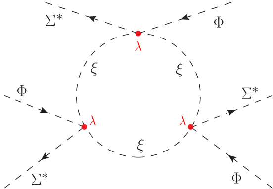
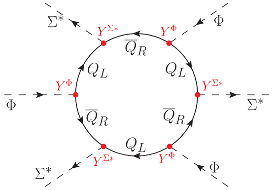
Figure 6: Examples of 1-PI one-loop diagrams that generate the quantum correction to the operator $\Phi^{3}\Sigma^{3*}$ and induce a parametric enhancement to its vacuum contribution. Couplings are shown in red for visual clarity.

Since all the couplings in Fig. 6 are renormalizable (and dimensionless), the diagrams are not associated to the EFT cutoff scale $\Lambda_{\rm UV}$ in any way; instead, the only scale involved other than the VEVs of $\Phi$ and $\Sigma$ are their masses of scale $V$ (the exception being the specific combination of entries corresponding to the SM Higgs). On dimensional grounds, the contributions to the vacuum from the operator $\mathcal{O}$ are schematically the following (ignoring any symmetry factors from diagrams):

$$\langle\mathcal{L}_{\mathcal{O}}+\delta\mathcal{L}_{\mathcal{O}}\rangle \sim C\,\frac{v^{6}}{\Lambda_{\rm UV}^{2}}+\frac{\lambda^{3}}{16\pi^{2}}\,\frac{v^{6}}{V^{2}}+\frac{(Y^{\Phi}Y^{\Sigma}{}^{*})^{3}}{16\pi^{2}}\,\frac{v^{6}}{V^{2}}+\text{h.c.}+\ldots\,,$$ (B.25)

where the 2nd and 3rd terms correspond to the quantum corrections and are parametrically enhanced relative to the tree-level term by a factor $\Lambda_{\rm UV}^{2}/V^{2}$. The dots at the end of the equation signify loop corrections in $\mathcal{L}_{\mathcal{O}}$ from diagrams not considered in this example.

In general, a quantum enhancement of a diagram can be inferred from counting powers of $\Lambda_{\rm UV}$ in the constituent couplings. If a loop diagram for a $d$-dimensional operator can be constructed from couplings of low enough mass dimension, the combined suppression in powers of $\Lambda_{\rm UV}$ may be less than the suppression $(\Lambda_{\rm UV})^{d-4}$ stemming from the tree-level EFT term. Factors of $\Lambda_{\rm UV}$ are instead replaced by the mass scale of the involved fields in the loops. The parametric enhancements in our model thus typically come in powers of $\Lambda_{\rm UV}/V$. In particular, a diagram constructed only out of renormalizable couplings does not have any power of the cutoff scale $\Lambda_{\rm UV}$ in the denominator, corresponding to an enhancement $(\Lambda_{\rm UV}/V)^{d-4}$.

Note that the example operator $\mathcal{O}$ does not violate PQ symmetry, cf. PQ charges in Table 1, so the quantum enhancement of its vacuum contribution has no impact on the axion potential, and is thus irrelevant for PQ quality. As stated earlier, a possible degradation of PQ quality would be analyzed by considering quantum corrections only to operators violating PQ and contributing to the vacuum already at tree level; for $d\leq 9$ they are listed in Table 6. Some considerations for such an analysis are the following:

• A loop diagram for a PQ-violating operator contains at least one PQ-violating vertex. This coupling may not necessarily come from an operator from the list in Table 6, since the vertex may also involve fermions, or it may be associated to a PQ-violating operator from the scalar potential with no direct contribution to the vacuum (an operator with vanishing all-VEV terms, and thus not considered in the tree-level analysis of PQ quality).

• Enhancements can occur in diagrams with an arbitrary number of loops, for operators up to arbitrary dimension $d$, and all possible couplings need to be considered (for a given operator up to its dimension $d$) — from the scalar potential, involving fermions, etc. The analysis is further complicated by having two scales $v$ and $V$, and beyond the diagrammatic level the detailed contraction of gauge indices also needs to be considered, similar to our tree-level analysis in App. B.3.1. At one loop, diagram topologies with a scalar or fermion loop can contribute, cf. examples of Fig. 6, while a gauge loop does not violate PQ; the scalar/fermion loop can have an arbitrary number of couplings lying on it.

• In the Pati-Salam model we consider, the lowest dimensional PQ-violating couplings (also among those involving fermions) are of dimension $d=6$. Therefore quantum corrections to any PQ-violating operator will have a suppression of at least $\Lambda_{\rm UV}^{2}$ in the denominator. On the other hand, each loop in a diagram will contribute a suppression factor $1/(16\pi^{2})$, implying that dangerous enhancements cannot come from an arbitrarily high number of loops. One can crudely estimate the number of loops $m$ that renders an enhanced contribution non-spoiling for PQ quality by comparing the vacuum contribution to the right-hand side of Eq. (2.26):

  $$\left(\frac{1}{16\pi^{2}}\right)^{m}\frac{v^{n}V^{6-n}}{\Lambda_{\rm UV}^{2}}\lesssim 10^{-10}\,\chi_{\rm QCD}^{4},$$ (B.26)

  where the denominator with $\Lambda_{\rm UV}$ is fixed to the worst case scenario (corresponding to the lowest-dimensional PQ-violating operator being the only non-renormalizable building block), and the power $n$ of EW VEVs varies based on the operator we are analyzing quantum contribution to. We assume no symmetry factors in diagrams and a tree-level EFT expansion with natural dimensionless coefficients in front of operators. Taking $V=10^{9}\,\mathrm{GeV}$ in Eq. (B.26) consistent with the high PQ quality scenario, the operators with powers $v^{0}$, $v^{2}$ and $v^{4}$ in the EW VEV need to be checked for enhancements only up to and including $13$, $7$, and $1$ loop(s), respectively, while operators yielding an EW VEV power $v^{n}$ for $n\geq 6$ will always be safe. Barring any other advantageous structural features of the model, such an analysis is clearly an enormously difficult task.

• An enhancement can be small enough in magnitude that it does not spoil PQ quality at all, or it may only somewhat degrade it. Although there is no general argument for the upper limit on $d$ of PQ-violating operators to be analyzed, those of larger $d$ come with more powers of suppression in $\Lambda_{\rm UV}$, and consequently the enhancement must be correspondingly larger to render the contribution PQ-spoiling. Heuristically we thus expect dangerous enhancements to be more likely for lower-dimensional operators.

More broadly, analogous considerations apply to any model of PQ quality, where the PQ-violating operator giving the largest contribution to the axion potential at tree level does not have the lowest mass dimension among all PQ-violating operators (including those involving fermions). Namely, the latter may not contribute directly, but as a building block in a loop diagram of another PQ-violating operator. Note also that a realistic model will always involve at least two scales, since it must involve both EW symmetry breaking at the scale $v$ and a different scale $V$ involved in PQ-breaking. In particular, PQ-violating operators involving fields with EW VEVs must be part of the analysis at the quantum level.

We finish by stating that while degradation of PQ quality from quantum corrections in our model is in principle possible, we are not aware of any specific dangerous contribution to this effect at the time of writing.

B.4 Computational framework for the Yukawa sector

This section presents the technical specifics of the Yukawa sector contributions, as discussed in Sect. 3, following the indexing conventions outlined in App. B.1. The content is systematically structured by topic for coherence:

1. Renormalizable operators:
   We explicitly express with indices some of the schematically written invariants from the main text, starting with the invariants from the renormalizable Yukawa sector in Eq. (2.1). The invariants are obtained with contarctions

   $$\epsilon_{i^{\prime}j^{\prime}}\;(\overline{Q}_{L})^{I}{}_{ai}\,(Q_{R})^{ai^{\prime}A}\,(\Phi^{\alpha})^{ij^{\prime}}{}_{A}\,,$$ (B.27)

   $$\epsilon_{i^{\prime}j^{\prime}}\;(\overline{Q}_{L})^{I}{}_{ai}\,(Q_{R})^{bi^{\prime}A}\,(\Sigma^{\alpha})^{a}{}_{b}{}^{ij^{\prime}}{}_{A}\,,$$ (B.28)

   $$(Q_{R})^{ai^{\prime}A}\,(Q_{R})^{bj^{\prime}B}\,(\Delta^{\ast})_{abi^{\prime}j^{\prime}AB}\,,$$ (B.29)

   where $I$ and $\alpha$ are the multiplicity indices and remain uncontracted. We assume one copy for $\Phi$ and two copies $\Sigma,\Sigma^{\prime}$. We denote by $\epsilon$ the anti-symmetric Levi-Civita tensor (of any rank). The results of Eqs. (3.7)–(3.9) and (3.12) follow from the above contractions, given the VEV definitions of App. B.1.

2. Leading non-renormalizable operators:
   The operators for leading non-renormalizable contributions have been determined by listing the invariants using the methods of App. B.2 and sorting by size of contribution. Those with leading contributions (unique in the entire range of $V$ given by Eq. (3.18)) are listed with non-tilde coefficients in Table 2. Suppressing gauge indices, we write their Lagrangian terms as

   $$-\mathcal{L}_{\Psi} \supset\sum_{I=1}^{3}\sum_{K=1}^{8}\frac{\mathcal{A}_{IK}}{\Lambda_{\rm UV}}\;(\overline{Q}_{L})^{I}(\Psi_{R})^{K}\Phi\chi$$

   $$\quad+\sum_{I=1}^{3}\sum_{K=1}^{8}\frac{2\sqrt{3}\,\mathcal{B}_{IK}}{\Lambda_{\rm UV}}\,(\overline{Q}_{L})^{I}(\Psi_{R})^{K}\Sigma\chi+\sum_{I=1}^{3}\sum_{K=1}^{8}\frac{2\sqrt{3}\,\mathcal{B}^{\prime}_{IK}}{\Lambda_{\rm UV}}\,(\overline{Q}_{L})^{I}(\Psi_{R})^{K}\Sigma^{\prime}\chi$$

   $$\quad+\sum_{K=1}^{8}\frac{\mathcal{C}_{K}}{\Lambda_{\rm UV}}\;Q_{R}(\Psi_{R})^{K}\,\Delta^{*}\chi+\sum_{K,N=1}^{8}\frac{1}{2}\frac{\mathcal{D}_{KN}}{\Lambda_{\rm UV}^{2}}\;(\Psi_{R})^{K}(\Psi_{R})^{N}\,\Delta^{*}\chi^{2}+\text{h.c.}.$$ (B.30)

   We see from Table 2 that each invariant has a unique gauge contraction; explicitly we take

   $$\mathcal{A}_{IK}: (\overline{Q}_{L})^{I}{}_{ai}\,(\Psi_{R})^{K}{}_{A}\,\Phi^{ii^{\prime}}{}_{B}\,\chi^{aj^{\prime}}{}_{C}\;\epsilon^{ABC}\,\epsilon_{i^{\prime}j^{\prime}}\,,$$ (B.31)

   $$\mathcal{B}_{IK}: (\overline{Q}_{L})^{I}{}_{ai}\,(\Psi_{R})^{K}{}_{A}\,\Sigma^{a}{}_{b}{}^{ii^{\prime}}{}_{B}\,\chi^{bj^{\prime}}{}_{C}\;\epsilon^{ABC}\,\epsilon_{i^{\prime}j^{\prime}}\,,$$ (B.32)

   $$\mathcal{C}_{K}: (Q_{R})^{ai^{\prime}D}\,(\Psi_{R})^{K}{}_{A}\,(\Delta^{\ast})_{abi^{\prime}j^{\prime}BD}\,\chi^{bj^{\prime}}{}_{C}\;\epsilon^{ABC}\,,$$ (B.33)

   $$\mathcal{D}_{KN}: (\Psi_{R})^{K}{}_{A}\,(\Psi_{R})^{N}{}_{D}\,(\Delta^{\ast})_{abi^{\prime}j^{\prime}BE}\,\chi^{ai^{\prime}}{}_{C}\,\chi^{bj^{\prime}}{}_{F}\;\epsilon^{ABC}\,\epsilon^{DEF}\,,$$ (B.34)

   and the $\mathcal{B}^{\prime}$-term is obtained from the $\mathcal{B}$-term by replacing $\Sigma\to\Sigma^{\prime}$.

3. Subleading non-renormalizable operators:
   We are interested in those subleading operators that involve the $\Psi_{0}$ anomalon modes defined in Eq. (3.20), since these states have been left out by the leading operators. For an operator consisting of a given set of fields, there may now be too many independent contractions of gauge indices to list. This problem is mitigated by considering only independent contractions in ${\rm SU}(3)_{f_{R}}$ flavor indices, in other words the independent contributions to the neutrino-anomalon mass matrix.

   The strategy to find the most important subleading contributions is as follows:

   1. We make use of the list of all operators up to $d=9$ involving a given pair of fermion fields. This has already been compiled for the purposes of determining leading operators. The list is ordered by the parametric size of the contribution to the mass for largest to smallest.

   2. We retain only those operators that can in principle contribute to the neutrino-anomalon masses based on Pati-Salam quantum numbers. Namely, in invariants all terms must have a vanishing total quantum number under any of the Pati-Salam diagonal generators, and this condition is checked for the term involving neutrinos/anomalons and VEVs. For irreps $\Phi,\Sigma,\Sigma^{\prime}$ with two EW VEVs, all possible combinations are considered in the search for a valid term.

   3. For each operator in the curated list we compute the number of different flavor contractions between VEVs — the same method as already used in App. B.3.1 — and then write down these contractions explicitly.

   4. For each contraction we check wether the contribution couples also to $\Psi_{0}$. This is trivially seen when the flavor index $A$ of the anomalon $(\Psi_{R})_{A}$ contracts with the $\chi$-VEV ${\color[rgb]{1.0,0,0}V}_{B}$ via the Levi-Civita tensor $\epsilon^{ABC}$.

   Carrying out the above strategy results in Table 7. For each type of contribution involving anomalons we list the subleading operators $\mathcal{O}$ that can contribute and all independent VEV contractions in flavor. The anomalon flavor indices for each block type, colored teal, are the following: ${\color[rgb]{0,.5,.5}A}$ for $L\Psi$, ${\color[rgb]{0,.5,.5}B}$ for $R\Psi$ and both ${\color[rgb]{0,.5,.5}A}$ and ${\color[rgb]{0,.5,.5}B}$ for $\Psi\Psi$. The contributions involving $\Psi_{0}$ (when the aforementioned index does not connect to a ${\color[rgb]{1.0,0,0}V}$-VEV via $\epsilon$) have a designated label, which is used for the coefficient of these relevant contributions in Table 2 and Eqs. (3.11)–(3.16). The listing of operators in the table is truncated, so that all largest subleading contributions up to the size when relevant contributions are first encountered are included. We took care to do this for all possible values of $V$ in Eq. (3.18), hence both the $v^{2}/\Lambda_{\rm UV}$ and $V^{5}/\Lambda_{\rm UV}^{4}$ contributions are present in the $\Psi\Psi$ block. We confirm the presence of each relevant contribution by specifying the corresponding index contraction explicitly (an example, there may be multiple yielding the same contribution):

   $$\tilde{\mathcal{A}}: (\overline{Q}_{L})^{I}{}_{ai}\,(\Psi_{R})^{K}{}_{A}\,\Delta^{abi^{\prime}j^{\prime}AB}\,(\Phi^{\ast})_{ji^{\prime}}{}^{C}\,(\chi^{*})_{bj^{\prime}}{}^{D}\;\epsilon_{BCD}\,\epsilon^{ij},$$ (B.35)

   $$\tilde{\mathcal{B}}: (\overline{Q}_{L})^{I}{}_{ai}\,(\Psi_{R})^{K}{}_{A}\,\Delta^{cbi^{\prime}j^{\prime}AB}\,(\Sigma^{\ast})_{c}{}^{a}{}_{ji^{\prime}}{}^{C}\,(\chi^{*})_{bj^{\prime}}{}^{D}\;\epsilon_{BCD}\,\epsilon^{ij},$$ (B.36)

   $$\tilde{\mathcal{C}}: (Q_{R})^{ai^{\prime}A}\,(\Psi_{R})^{N}{}_{B}\,\Delta^{cdk^{\prime}l^{\prime}EF}\,\Delta^{*}_{cdk^{\prime}l^{\prime}ED}\,\Delta^{*}_{abi^{\prime}j^{\prime}AC}\,\chi^{bj^{\prime}}{}_{F}\;\epsilon^{BCD},$$ (B.37)

   $$\tilde{\mathcal{D}}: (\Psi_{R})^{K}{}_{A}\,(\Psi_{R})^{N}{}_{B}\,\Phi^{\ast}{}_{ii^{\prime}}{}^{A}\,\Phi^{\ast}{}_{jj^{\prime}}{}^{B}\;\epsilon^{ij}\,\epsilon^{i^{\prime}j^{\prime}},$$ (B.38)

   $$\tilde{\mathcal{E}}: (\Psi_{R})^{K}{}_{A}\,(\Psi_{R})^{N}{}_{B}\,\Sigma^{\ast}{}_{a}{}^{b}{}_{ii^{\prime}}{}^{A}\,\Sigma^{\ast}{}_{b}{}^{a}{}_{jj^{\prime}}{}^{B}\;\epsilon^{ij}\,\epsilon^{i^{\prime}j^{\prime}},$$ (B.39)

   $$\tilde{\mathcal{F}}: (\Psi_{R})^{K}{}_{A}\,(\Psi_{R})^{N}{}_{B}\,\Delta^{cdk^{\prime}l^{\prime}GH}\,\Delta^{\ast}_{cdk^{\prime}l^{\prime}CE}\,\Delta^{\ast}_{abi^{\prime}j^{\prime}DF}\,\chi^{ai^{\prime}}{}_{G}\,\chi^{bj^{\prime}}{}_{H}\;\epsilon^{ACD}\,\epsilon^{BEF},$$ (B.40)

   $$\tilde{\mathcal{G}}: (\Psi_{R})^{K}{}_{A}\,(\Psi_{R})^{N}{}_{B}\,\Delta^{cdk^{\prime}l^{\prime}GH}\,\Delta^{\ast}_{cdk^{\prime}l^{\prime}GD}\,\Delta^{\ast}_{abi^{\prime}j^{\prime}CE}\,\chi^{ai^{\prime}}{}_{H}\,\chi^{bj^{\prime}}{}_{F}\;\epsilon^{DEF}\,\epsilon^{ABC}.$$ (B.41)

   type	$\mathcal{O}$	$\sim\langle\mathcal{O}\rangle$	$\#_{f_{R}}$	${\rm SU}(3)_{f_{R}}$ VEV contractions	label
   $(L\Psi)_{{\color[rgb]{0,.5,.5}A}}$	$\overline{Q}_{L}\Psi_{R}\Phi\chi\xi$	$vV^{2}/\Lambda_{\rm UV}^{2}$	$1$	$\epsilon^{{\color[rgb]{0,.5,.5}A}BC}\,{\color[rgb]{0,0,1}v^{u\Phi}_{{\color[rgb]{0,0,0}B}}}{\color[rgb]{1.0,0,0}W}{\color[rgb]{1.0,0,0}V}_{C}$	—
   	$\overline{Q}_{L}\Psi_{R}\Sigma\chi\xi$	$vV^{2}/\Lambda_{\rm UV}^{2}$	$1$	$\epsilon^{{\color[rgb]{0,.5,.5}A}BC}\,{\color[rgb]{0,0,1}v^{u\Sigma}_{{\color[rgb]{0,0,0}B}}}{\color[rgb]{1.0,0,0}W}{\color[rgb]{1.0,0,0}V}_{C}$	—
   	$\overline{Q}_{L}\Psi_{R}\Phi^{*}\Delta\chi^{*}$	$vV^{2}/\Lambda_{\rm UV}^{2}$	$1$	${\color[rgb]{1.0,0,0}Z^{{\color[rgb]{0,0,0}{\color[rgb]{0,.5,.5}A}B}}}\,\epsilon_{BCD}\,({\color[rgb]{0,0,1}v^{\ast d\Phi}})^{{\color[rgb]{0,0,0}C}}{\color[rgb]{1.0,0,0}V^{\ast}}{}^{D}$	$\tilde{\mathcal{A}}$
   	$\overline{Q}_{L}\Psi_{R}\Sigma^{*}\Delta\chi^{*}$	$vV^{2}/\Lambda_{\rm UV}^{2}$	$1$	${\color[rgb]{1.0,0,0}Z^{{\color[rgb]{0,0,0}{\color[rgb]{0,.5,.5}A}B}}}\,\epsilon_{BCD}\,({\color[rgb]{0,0,1}v^{\ast d\Sigma}})^{{\color[rgb]{0,0,0}C}}{\color[rgb]{1.0,0,0}V^{\ast}}{}^{D}$	$\tilde{\mathcal{B}}$
   $(R\Psi)^{A}{}_{{\color[rgb]{0,.5,.5}B}}$	$Q_{R}\Psi_{R}\Delta^{*}\chi\xi$	$V^{3}/\Lambda_{\rm UV}^{2}$	$1$	$\epsilon^{{\color[rgb]{0,.5,.5}B}CD}\,{\color[rgb]{1.0,0,0}Z^{\ast}_{{\color[rgb]{0,0,0}AC}}}{\color[rgb]{1.0,0,0}V}_{D}{\color[rgb]{1.0,0,0}W}$	—
   	$Q_{R}\Psi_{R}\Delta\Delta^{*2}\chi$	$V^{4}/\Lambda_{\rm UV}^{3}$	$3$	$\epsilon^{{\color[rgb]{0,.5,.5}B}CD}\,{\color[rgb]{1.0,0,0}Z^{{\color[rgb]{0,0,0}EF}}}{\color[rgb]{1.0,0,0}Z^{\ast}_{{\color[rgb]{0,0,0}EF}}}{\color[rgb]{1.0,0,0}Z^{\ast}_{{\color[rgb]{0,0,0}AC}}}{\color[rgb]{1.0,0,0}V}_{D}$	—
   				$\epsilon^{{\color[rgb]{0,.5,.5}B}CD}\,{\color[rgb]{1.0,0,0}Z^{{\color[rgb]{0,0,0}EF}}}{\color[rgb]{1.0,0,0}Z^{\ast}_{{\color[rgb]{0,0,0}EA}}}{\color[rgb]{1.0,0,0}Z^{\ast}_{{\color[rgb]{0,0,0}FC}}}{\color[rgb]{1.0,0,0}V}_{D}$	—
   				$\epsilon^{{\color[rgb]{0,.5,.5}B}CD}\,{\color[rgb]{1.0,0,0}Z^{{\color[rgb]{0,0,0}EF}}}{\color[rgb]{1.0,0,0}Z^{\ast}_{{\color[rgb]{0,0,0}ED}}}{\color[rgb]{1.0,0,0}Z^{\ast}_{{\color[rgb]{0,0,0}AC}}}{\color[rgb]{1.0,0,0}V}_{F}$	$\tilde{\mathcal{C}}$
   	$Q_{R}\Psi_{R}\Delta^{*}\chi^{2}\chi^{*}$	$V^{4}/\Lambda_{\rm UV}^{3}$	$2$	$\epsilon^{{\color[rgb]{0,.5,.5}B}CD}\,{\color[rgb]{1.0,0,0}Z^{\ast}_{{\color[rgb]{0,0,0}AC}}}{\color[rgb]{1.0,0,0}V}_{D}{\color[rgb]{1.0,0,0}V}_{E}{\color[rgb]{1.0,0,0}V^{\ast}}{}^{E}$	—
   				$\epsilon^{{\color[rgb]{0,.5,.5}B}CD}\,{\color[rgb]{1.0,0,0}Z^{\ast}_{{\color[rgb]{0,0,0}DE}}}{\color[rgb]{1.0,0,0}V}_{A}{\color[rgb]{1.0,0,0}V}_{C}{\color[rgb]{1.0,0,0}V^{\ast}}{}^{E}$	—
   	$Q_{R}\Psi_{R}\Delta^{*}\chi\xi^{2}$	$V^{4}/\Lambda_{\rm UV}^{3}$	$1$	$\epsilon^{{\color[rgb]{0,.5,.5}B}CD}\,{\color[rgb]{1.0,0,0}Z^{\ast}_{{\color[rgb]{0,0,0}AC}}}{\color[rgb]{1.0,0,0}V}_{D}{\color[rgb]{1.0,0,0}W}^{2}$	—
   $(\Psi\Psi)_{{\color[rgb]{0,.5,.5}A}{\color[rgb]{0,.5,.5}B}}$	$\Psi_{R}\Psi_{R}\Phi^{*2}$	$v^{2}/\Lambda_{\rm UV}$	$1$	$({\color[rgb]{0,0,1}v^{u\Phi}}^{\ast})^{{\color[rgb]{0,.5,.5}A}}({\color[rgb]{0,0,1}v^{d\Phi}}^{\ast})^{{\color[rgb]{0,.5,.5}B}}+[{\color[rgb]{0,.5,.5}A}\leftrightarrow{\color[rgb]{0,.5,.5}B}]$	$\tilde{\mathcal{D}}$
   	$\Psi_{R}\Psi_{R}\Sigma^{*2}$	$v^{2}/\Lambda_{\rm UV}$	$1$	$({\color[rgb]{0,0,1}v^{u\Sigma}}^{\ast})^{{\color[rgb]{0,.5,.5}A}}({\color[rgb]{0,0,1}v^{d\Sigma}}^{\ast})^{{\color[rgb]{0,.5,.5}B}}+[{\color[rgb]{0,.5,.5}A}\leftrightarrow{\color[rgb]{0,.5,.5}B}]$	$\tilde{\mathcal{E}}$
   	$\Psi_{R}\Psi_{R}\Delta^{*}\chi^{2}\xi$	$V^{4}/\Lambda_{\rm UV}^{3}$	$1$	$\epsilon^{{\color[rgb]{0,.5,.5}A}CD}\epsilon^{{\color[rgb]{0,.5,.5}B}EF}\,{\color[rgb]{1.0,0,0}Z^{\ast}_{{\color[rgb]{0,0,0}CE}}}{\color[rgb]{1.0,0,0}V}_{D}{\color[rgb]{1.0,0,0}V}_{F}{\color[rgb]{1.0,0,0}W}$	—
   	$\Psi_{R}\Psi_{R}\Delta\Delta^{*2}\chi^{2}$	$V^{5}/\Lambda_{\rm UV}^{4}$	$5$	$\epsilon^{{\color[rgb]{0,.5,.5}A}CD}\epsilon^{{\color[rgb]{0,.5,.5}B}EF}\,{\color[rgb]{1.0,0,0}Z^{{\color[rgb]{0,0,0}GH}}}{\color[rgb]{1.0,0,0}Z^{\ast}_{{\color[rgb]{0,0,0}GH}}}{\color[rgb]{1.0,0,0}Z^{\ast}_{{\color[rgb]{0,0,0}CE}}}{\color[rgb]{1.0,0,0}V}_{D}{\color[rgb]{1.0,0,0}V}_{F}$	—
   				$\epsilon^{{\color[rgb]{0,.5,.5}A}CD}\epsilon^{{\color[rgb]{0,.5,.5}B}EF}\,{\color[rgb]{1.0,0,0}Z^{{\color[rgb]{0,0,0}GH}}}{\color[rgb]{1.0,0,0}Z^{\ast}_{{\color[rgb]{0,0,0}GC}}}{\color[rgb]{1.0,0,0}Z^{\ast}_{{\color[rgb]{0,0,0}HE}}}{\color[rgb]{1.0,0,0}V}_{D}{\color[rgb]{1.0,0,0}V}_{F}$	—
   				$\epsilon^{{\color[rgb]{0,.5,.5}A}CD}\epsilon^{{\color[rgb]{0,.5,.5}B}EF}\,{\color[rgb]{1.0,0,0}Z^{{\color[rgb]{0,0,0}GH}}}{\color[rgb]{1.0,0,0}Z^{\ast}_{{\color[rgb]{0,0,0}CE}}}{\color[rgb]{1.0,0,0}Z^{\ast}_{{\color[rgb]{0,0,0}DF}}}{\color[rgb]{1.0,0,0}V}_{G}{\color[rgb]{1.0,0,0}V}_{H}$	$\tilde{\mathcal{F}}$
   				$\epsilon^{{\color[rgb]{0,.5,.5}A}CD}\epsilon^{{\color[rgb]{0,.5,.5}B}EF}\,{\color[rgb]{1.0,0,0}Z^{{\color[rgb]{0,0,0}GH}}}{\color[rgb]{1.0,0,0}Z^{\ast}_{{\color[rgb]{0,0,0}GC}}}{\color[rgb]{1.0,0,0}Z^{\ast}_{{\color[rgb]{0,0,0}DE}}}{\color[rgb]{1.0,0,0}V}_{H}{\color[rgb]{1.0,0,0}V}_{F}$	—
   				$\epsilon^{{\color[rgb]{0,.5,.5}AB}C}\epsilon^{DEF}\,{\color[rgb]{1.0,0,0}Z^{{\color[rgb]{0,0,0}GH}}}{\color[rgb]{1.0,0,0}Z^{\ast}_{{\color[rgb]{0,0,0}GD}}}{\color[rgb]{1.0,0,0}Z^{\ast}_{{\color[rgb]{0,0,0}CE}}}{\color[rgb]{1.0,0,0}V}_{H}{\color[rgb]{1.0,0,0}V}_{F}$	$\tilde{\mathcal{G}}$
   	$\Psi_{R}\Psi_{R}\Delta^{*}\chi^{3}\chi^{*}$	$V^{5}/\Lambda_{\rm UV}^{4}$	$1$	$\epsilon^{{\color[rgb]{0,.5,.5}A}CD}\epsilon^{{\color[rgb]{0,.5,.5}B}EF}\,{\color[rgb]{1.0,0,0}Z^{\ast}_{{\color[rgb]{0,0,0}CE}}}{\color[rgb]{1.0,0,0}V}_{D}{\color[rgb]{1.0,0,0}V}_{F}\,{\color[rgb]{1.0,0,0}V}_{G}{\color[rgb]{1.0,0,0}V^{\ast}}{}^{G}$	—
   	$\Psi_{R}\Psi_{R}\Delta^{*}\chi^{2}\xi^{2}$	$V^{5}/\Lambda_{\rm UV}^{4}$	$1$	$\epsilon^{{\color[rgb]{0,.5,.5}A}CD}\epsilon^{{\color[rgb]{0,.5,.5}B}EF}\,{\color[rgb]{1.0,0,0}Z^{\ast}_{{\color[rgb]{0,0,0}CE}}}{\color[rgb]{1.0,0,0}V}_{D}{\color[rgb]{1.0,0,0}V}_{F}{\color[rgb]{1.0,0,0}W}^{2}$	—

   Table 7: The list of subleading contributions from largest to smallest for all blocks in (3.10) involving anomalons: $L\Psi$, $R\Psi$, $\Psi\Psi$ involving anomalons we list the subleading operators $\mathcal{O}$ that can contribute. The operator (in terms of field powers) is denoted by $\mathcal{O}$, its VEV scaling by $\sim\langle\mathcal{O}\rangle$ and the number of independent contributions to the mass (number of independent flavor contractions) by $\#_{f_{R}}$, which are then listed explicitly in different rows. Contributions that involve $\Psi_{0}$ anomalon states from Eq. (3.20) have a label next to them, and are included as relevant contributions into Table 2 and Eqs. (3.11)–(3.16). The flavor indices of anomalons in the first column and the associated free indices in the contraction column are colored teal as visual emphasis due to their structural importance, see main text; the standard color coding of blue for EW VEVs and red for the PQ-breaking Pati-Salam VEVs is also used.

4. Redundancy removal:
   We address here the redundancy in describing the Yukawa sector of our Pati-Salam model. The SM fermions are packed into two types of representations, namely $Q_{L}$ and $Q_{R}$, thus allowing for a global flavor transformation $\mathrm{U}(3)_{Q_{L}}\times\mathrm{U}(3)_{Q_{R}}$, transforming the multiplicity index $I$ and the gauged family index $A$ with the two respective factors. The second factor essentially contains the ${\rm SU}(3)_{f_{R}}$ gauge transformations.

   An $\mathrm{SU}(3)$ transformation acting on a set of complex vectors $\vec{v}_{i}=(x_{i},y_{i},z_{i})$ can bring one into the form $\vec{v}_{1}=(0,0,z_{1})$ and a subsequent $\mathrm{SU}(2)$ rotation in the first two components can bring a second vector to the form $\vec{v}_{2}=(0,y_{2},z_{2})$ without disrupting the form of $\vec{v}_{1}$. The VEV component $z_{1},y_{2}\in\mathbb{R}$ and $z_{2}\in\mathbb{C}$ in accordance with using the $8$ real degrees of freedom of ${\rm SU}(3)$ to remove the same number in $\vec{v}_{1}$ and $\vec{v}_{2}$.

   The rotation $\mathrm{U}(3)_{Q_{L}}$ can be used on the parameters of the renormalizable Yukawa potential, where we have a set of $3$ vectors $\{Y^{\Phi}_{I},Y^{\Sigma}_{I},Y^{\Sigma^{\prime}}_{I}\}$, while the $\mathrm{U}(3)_{Q_{R}}$ rotation can be used on the set of the $6$ vectors of EW VEVs listed in Eq. (3.1). In particular, we find the removal of redundancies via the choice of Eq. (3.6) the most convenient, especially when addressing the realistic nature of the Yukawa sector in Sect. 3.3.

5. Diagonalization of a hierarchical mass matrix:
   To obtain masses and mixings, the matrix of Eq. (3.24) is diagonalized via Takagi decomposition. A general complex symmetric matrix $\mathbf{M}$ can be decomposed as

   $$\mathbf{M} =\mathbf{U}\mathbf{D}\mathbf{U}^{T}\,,$$ (B.42)

   where $\mathbf{D}$ is diagonal with non-negative real eigenvalues $m_{i}\equiv D_{ii}$, and $\mathbf{U}$ is a unitary matrix. The decomposition can be performed numerically, but an analytic approximation is also possible due to the hierarchical nature of our mass matrix. We elaborate on the general methods involving the analytic approach:

   1. Consider a real matrix $\mathbf{M}$ to avoid unnecessarily complicated expressions; $\mathbf{U}$ then becomes real and orthogonal. Assuming parametrically small off-diagonal entries in $\mathbf{M}$, and consistently expanding order-by-order in these small parameters, one can derive the following approximations for masses and mixing angles at next-to-leading order:

      $$m_{i} \approx M_{ii}+\sum_{k\neq i}\frac{M_{ik}^{2}}{M_{ii}-M_{kk}}\,, \quad U_{ij} \approx\frac{M_{ij}}{M_{jj}-M_{ii}}-\sum_{k\neq i,j}\frac{M_{ik}M_{jk}}{(M_{jj}-M_{ii})(M_{kk}-M_{jj})}\,,$$ (B.43)

      where $M_{ij}$ are the components of $\mathbf{M}$, and $U_{ij}$ are off-diagonal elements of $\mathbf{U}$ for $i<j$ (note that the expression is not $i\leftrightarrow j$ symmetric). Orthogonality of $\mathbf{U}$ implies that specifying the upper-diagonal part uniquely determines the entire matrix, which can be reconstructed as follows:

      $$(\mathbf{U})_{ij} \approx\begin{cases}U_{ij}&;\quad i<j\\[3.0pt] -U_{\{ij\}}-\sum_{k\neq i,j}(-1)^{H_{i-k}+H_{j-k}}\,U_{\{ik\}}U_{\{jk\}}&;\quad i>j\\[3.0pt] 1-\sum_{k\neq i}U_{\{ik\}}^{2}/2&;\quad i=j\\ \end{cases}\,,$$ (B.44)

      where curly brackets $\{\}$ order the indices from smaller to larger, and $H$ is the Heaviside function ($H_{x}=1$ for $x\geq 0$ and $H_{x}=0$ for $x<0$).

   2. Note that the expressions of Eq. (B.43) fail if denominators blow up. Assuming non-degenerate eigenvalues, the main mode of failure is when (multiple) diagonal entries $M_{ii}$ are also parametrically small. For rough estimates, Eq. (B.43) can be modified to incorporate the possibility of small diagonal entries $M_{ii}$ by replacing them in denominators by the mass eigenvalues $m_{i}$:

      $$m_{i} \sim M_{ii}+\sum_{k\neq i}\frac{M_{ik}^{2}}{m_{i}-m_{k}}\,, \quad U_{ij} \sim\frac{1}{m_{j}-m_{i}}\;\left(M_{ij}-\sum_{k\neq i,j}\frac{M_{ik}M_{jk}}{m_{k}-m_{j}}\right)\,.$$ (B.45)

      One can solve this system by computing $m_{i}$ iteratively until consistent, starting with $m_{i}=M_{ii}$, and then using these quantities for the mixing $U_{ij}$. Finally, any violation of $U_{ij}\ll 1$ is a sign that the method is not applicable, since parametric smallness of mixing was the starting assumption.

B.5 Perturbativity

With the introduction of a horizontal gauge symmetry, i.e. the gauged flavor group $\mathrm{SU}(3)_{f_{R}}$, the number of field degrees of freedom in the scalar sector increases, since many will transform non-trivially under it. For our particular model, we can see from Table 1 that all scalar fields transform non-trivially under the flavor group.

The proliferation of degrees of freedom brings concerns regarding the perturbativity of the model. One aspect of this is the behavior of gauge couplings $g_{i}$ above the Pati-Salam scale.

Writing the renormalization group equations (RGE) in terms of $\alpha_{i}^{-1}\equiv 4\pi/g_{i}^{2}$, the two loop RGE take the well-known form (see e.g. [161, 162])

$$\dfrac{d}{dt}\,\alpha^{-1}_{i} =-\dfrac{1}{2\pi}\big{(}a_{i}+\dfrac{1}{4\pi}\sum_{j}b_{ij}\alpha_{j}\big{)}\,,$$ (B.46)

with $t=\log(\mu/\mu_{0})$ and $\mu_{0}$ being a reference scale. We retained in the beta function only the gauge contributions, since they dominate over the Yukawa contributions.

We use the following conventions: we label the SM gauge couplings $\alpha$ by $(\alpha_{3},\alpha_{2},\alpha_{1})$ referring to each factor of ${\rm SU}(3)_{C}\times{\rm SU}(2)_{L}\times\mathrm{U}(1)_{Y}$ from left to right, and we use $(\alpha_{4C},\alpha_{2L},\alpha_{2R},\alpha_{3F})$ in the Pati-Salam model ${\rm SU}(4)_{C}\times{\rm SU}(2)_{L}\times{\rm SU}(2)_{R}\times{\rm SU}(3)_{f_{R}}$.

The coefficients $a_{i}$ and $b_{ij}$ can be computed in the standard way [163]. Referring with the index $i$ to group factors from left to right using the conventions above, the SM coefficients are

$$a^{\text{(SM)}}_{i} =(-7,-\tfrac{19}{6},\tfrac{41}{10})\,, b^{\text{(SM})}_{ij} =\begin{pmatrix}-26&\tfrac{9}{2}&\frac{11}{10}\\ 12&\tfrac{35}{6}&\frac{9}{10}\\ \tfrac{44}{5}&\tfrac{27}{10}&\tfrac{199}{50}\\ \end{pmatrix}\,,$$ (B.47)

while the Pati-Salam model with the fermion and scalar content of Table 1, and taking $N_{\Phi}=1$ and $N_{\Sigma}=2$, yields the the 1- and 2-loop beta coefficients

$$a^{\text{(PS)}}_{i} =(\tfrac{127}{3},\tfrac{83}{3},\tfrac{224}{3},\tfrac{124}{3})\,, b^{\text{(PS)}}_{ij} =\begin{pmatrix}\tfrac{8915}{3}&\tfrac{585}{2}&\tfrac{1563}{2}&1256\\[3.0pt] \tfrac{2925}{2}&\tfrac{1220}{3}&279&496\\[3.0pt] \tfrac{7815}{2}&279&\tfrac{5078}{3}&2144\\[3.0pt] 2355&186&804&\tfrac{4900}{3}\\[3.0pt] \end{pmatrix}\,.$$ (B.48)

The hypercharge is embedded into the Pati-Salam group via

$$\tfrac{1}{2}\,Y=\tfrac{1}{2}(B-L)+t^{3}_{R}=\sqrt{\tfrac{2}{3}}\,t^{15}_{C}+t^{3}_{R}\,,$$ (B.49)

where $t^{15}_{C}=\tfrac{1}{\sqrt{24}}\,\mbox{diag}\,(1,1,1,-3)$ and $t^{3}_{R}=\tfrac{1}{2}\,\mbox{diag}\,(1,-1)$ are diagonal generators in ${\rm SU}(4)_{C}$ and ${\rm SU}(2)_{R}$, respectively, and $B$ and $L$ are baryon and lepton number. This connection yields the matching condition at the Pati-Salam scale to be

$$(\alpha^{-1}_{4C},\;\alpha^{-1}_{2L},\;\alpha^{-1}_{2R}) =(\alpha^{-1}_{3},\;\alpha^{-1}_{2},\;\tfrac{5}{3}\alpha^{-1}_{1}-\tfrac{2}{3}\alpha^{-1}_{3}).$$ (B.50)

The flavor gauge coupling $\alpha_{F}$ is not determined through these, since no remnant of ${\rm SU}(3)_{f_{R}}$ is embedded into the SM group.

Eqs. (B.46)–(B.48) and (B.50) enable a full bottom-up RGE evolution of gauge couplings, starting with SM values at the $Z$-scale [164, 165, 166, 167, 168]:

$$\big{(}\alpha^{-1}_{3},\;\alpha^{-1}_{2},\;\alpha^{-1}_{1}\big{)}(M_{Z}) =(8.550\pm 0.065,\;29.6261\pm 0.0051,\;59.1054\pm 0.0031).$$ (B.51)

The only unknowns are the matching scale $\mu_{PS}$ (where we assume to be all the non-SM fields of the model, neglecting threshold effects) and the flavor gauge coupling $\alpha_{3F}^{-1}(\mu_{PS})$ at that scale, where $\mu_{PS}\sim V\sim 10^{9}\,\mathrm{GeV}$.

A benchmark example with $\alpha^{-1}_{3F}(\mu_{PS})=50$ is shown in the left panel in Fig. 7. It captures the salient feature that the coupling $\alpha_{4C}$ is the one driven to a Landau pole at $\mu_{L}$, i.e., $\alpha_{4C}^{-1}(\mu_{L})=0$, unless the coupling $\alpha_{3F}$ is large. Changing the coupling values for $\alpha_{3F}$ has only a slight effect on $\mu_{L}$, since it drives the other couplings only through the two-loop cross-term.

With a rising matching scale $\mu_{PS}$, the value $\alpha_{4C}^{-1}$ at that scale rises, while $\alpha_{2R}^{-1}$ decreases, as it can be deduced from the left panel of Fig. 7. A higher value of $\alpha_{4C}^{-1}$ then implies more running needed before reaching a Landau pole, as seen in the right panel. Beyond around $\mu_{PS}\sim 10^{11.2}\,\mathrm{GeV}$, however, the change of trend is due to $\alpha^{-1}_{2R}$ reaching the Landau pole before $\alpha_{4C}^{-1}$ does.

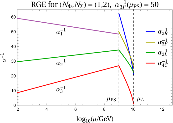
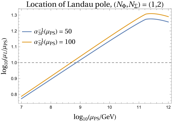
Figure 7: Gauge coupling running for a benchmark point with $\alpha_{3F}^{-1}=50$ at the scale $\mu_{PS}$ (left panel), and the effect of the matching scale $\mu_{PS}$ and the value of the flavor gauge coupling $\alpha_{3F}^{-1}(\mu_{PS})$ on the position of the Landau pole at scale $\mu_{L}$ (right panel).

We thus see that the gauge couplings have a Landau pole around one order of magnitude above the matching scale, i.e. $\log_{10}(\mu_{L}/\mu_{PS})\simeq 1$. Some non-renormalizable operators are thus expected to be suppressed only by a factor $10^{-1}$, which we still deem acceptable for the theory to be treated perturbatively at the scale $\mu_{PS}$.

On the other hand, the existence of a Landau pole before the Planck scale raises a more conceptual issue. Unless the theory is tempered by non-perturbative dynamics arising before $\mu_{L}$, the latter scale should be associated to some new physics which ensures a proper UV behaviour. We then need to require that such new physics does not break the PQ symmetry, since our working hypothesis is that the scale responsible for the PQ-breaking operators is $\Lambda_{\rm UV}\sim M_{\rm Pl}$.

Finally, we observe that the issue of perturbativity and the Landau pole arising before the Planck scale should generically arise in models with gauged horizontal symmetries, and it is thus not exclusive for the models under investigation in this paper.

Appendix C Reflections on the ${\rm SO}(10)\times{\rm SU}(3)_{f}$ model of Ref. [1]

In this Appendix we reflect on the ${\rm SO}(10)\times{\rm SU}(3)_{f}$ model from [1], which served as the original inspiration for the Pati-Salam model of this paper, provide some corrections to the analysis in Ref. [1] and compare the two models.

C.1 Comparing the ${\rm SO}(10)$ and Pati-Salam models

The ${\rm SO}(10)\times{\rm SU}(3)_{f}$ model of Ref. [1] features the field content listed for convenience in Table 8. The fermions are generically labeled by $\psi$ and the scalars by $\phi$. This compares to the Pati-Salam case of Table 1 as follows:

• The fermions $Q_{L}$ and $Q_{R}$ now join into a single representation $\phi_{16}$. The flavor group now simultaneously rotates both $Q_{L}$ and $Q_{R}$, so we label it simply as ${\rm SU}(3)_{f}$.

• The exotic fermions in light gray ensure ${\rm SU}(3)_{f}$ anomaly cancellation, in analogy with $\Psi_{R}$ canceling ${\rm SU}(3)_{f_{R}}$ anomalies.

• Ignoring the flavor assignment and considering only the inclusion ${\rm SU}(4)_{\rm PS}\times{\rm SU}(2)_{L}\times{\rm SU}(2)_{R}\subset{\rm SO}(10)$, we have

  $$\Phi \subset\phi_{10}\,, \Sigma,\Delta \subset\phi_{\overline{126}}\,, \chi^{\ast} \subset\phi_{16}\,.$$ (C.1)

  The representations $\phi_{10}$ and $\phi_{\overline{126}}$ function as containers for the SM Higgs, the same as $\Phi$ and $\Sigma$. The representations $\phi_{\overline{126}}$ is also crucial for neutrino masses, analogously to $\Delta$.

• More loosely, one can draw an analogy between $\chi$ and $\phi_{16}$, as well as between the real representations $\xi$ and $\phi_{45}$. Although the details slightly differ between the models, both pairs are involved in breaking the gauge symmetry to the SM, and only in the presence of both representations there is an accidental $\mathrm{U}(1)_{\rm PQ}$ not aligned with $B-L$.

• The action under the center $\mathbb{Z}_{4}$ of ${\rm SO}(10)$ does not directly correspond to the action of the $\mathbb{Z}_{4}$ center of ${\rm SU}(4)_{\rm PS}$. In particular, the PS center acts differently on $\Phi$ and $\Sigma$ compared to how the ${\rm SO}(10)$-center acts on the their parent irreps $\phi_{10}$ and $\phi_{\overline{126}}$; for the Peccei-Quinn symmetry and its quality to behave similarly, the transformation of the PS irreps under flavor was thus modified compared to the ${\rm SO}(10)$ case.

$$\begin{array}[]{c|c|cc|cc|c|c}\hbox{Field}&\hbox{Lorentz}&{\rm SO}(10)&\mathbb{Z}_{4}&{\rm SU}(3)_{f}&\mathbb{Z}_{3}&\text{Generations}&{\rm U}(1)_{\rm PQ}\\ \hline\cr\psi_{16}&(1/2,0)&16&+i&{\textbf{3}}&e^{i2\pi/3}&1&+1\\ \psi_{1}&(1/2,0)&1&+1&\overline{{\textbf{3}}}&e^{i4\pi/3}&16&\phantom{+}0\\ \hline\cr\phi_{10}&(0,0)&10&-1&\overline{\textbf{6}}&e^{i2\pi/3}&1&-2\\ \phi_{16}&(0,0)&16&i&\overline{{\textbf{3}}}&e^{i4\pi/3}&1&-1\\ \phi_{\overline{126}}&(0,0)&\overline{126}&-1&\overline{\textbf{6}}&e^{i2\pi/3}&1&-2\\ \phi_{45}&(0,0)&45&1&{\textbf{1}}&1&1&0\\ \end{array}$$

Table 8: Field content of the ${\rm SO}(10)$ model with gauged flavor from [1]. For each irrep we state its transformation properties under ${\rm SO}(10)$ and ${\rm SU}(3)_{f}$, their respective centers $\mathbb{Z}_{4}$ and $\mathbb{Z}_{3}$, and under the accidental ${\rm U}(1)_{\rm PQ}$.

C.2 The scalar potential of the ${\rm SO}(10)$ model

We provide here some errata regarding the operators in the scalar potential of the ${\rm SO}(10)$ model from [1], although the main conclusion regarding the emergence of the accidental ${\rm U}(1)_{\rm PQ}$ symmetry remains unchanged. The renormalizable potential of the ${\rm SO}(10)$ model, as determined by the methods of App. B.2, consists of the following invariants:

$$\tilde{\mathcal{V}} =\tilde{\mathcal{V}}_{2}+\tilde{\mathcal{V}}_{3}+\tilde{\mathcal{V}}_{4}+\tilde{\mathcal{V}}_{\mathbb{C}}\,,$$ (C.2)

$$\tilde{\mathcal{V}}_{2} =|\phi_{10}|^{2}+|\phi_{\overline{126}}|^{2}+|\phi_{16}|^{2}+\phi_{45}^{2}\,,$$ (C.3)

$$\tilde{\mathcal{V}}_{3} =\left(|\phi_{10}|^{2}+|\phi_{\overline{126}}|^{2}+|\phi_{16}|^{2}\right)\phi_{45}\,,$$ (C.4)

$$\tilde{\mathcal{V}}_{4} =\left(|\phi_{10}|^{2}+|\phi_{\overline{126}}|^{2}+|\phi_{16}|^{2}+\phi_{45}^{2}\right)^{2}\,,$$ (C.5)

$$\tilde{\mathcal{V}}_{\mathbb{C}} =\phi_{10}\phi_{16}^{\ast 2}\,(1+\phi_{45})+\phi_{10}\phi_{\overline{126}}^{\ast}\left(\phi_{10}\phi_{\overline{126}}^{\ast}+|\phi_{\overline{126}}|^{2}+|\phi_{16}|^{2}+\phi_{45}^{2}\right)+\text{h.c.}\,.$$ (C.6)

The symbols $\mathcal{V}$ carry a tilde on top to distinguish them from the scalar potential of the PS model from Sect. 2.

Note that two more types of invariants are in principle possible from the given irreps: $\phi_{45}^{3}$ and $\phi_{16}^{2}\phi_{\overline{126}}^{\ast}\phi_{45}$. These, however, are anti-symmetric with respect to the same-irrep factors, and thus identically vanish given that the multiplicity of all scalar irreps in Table 8 is $1$, i.e., one needs to consider the criteria for invariants all the way up to condition 3 in App. B.2. While [1] does not list the invariants of $\tilde{\mathcal{V}}_{3}$ and the last two terms of $\tilde{\mathcal{V}}_{4}$, these clearly have no impact on the preservation of $\mathrm{U}(1)_{\rm PQ}$ from Table 8, so the associated conclusions are unchanged.

Using the methods of App. B.2 up to condition 2, we also list the invariants that break PQ symmetry and potentially contribute to the vacuum, analogously to our analysis in Sect. 2.3. The potentially dangerous invariants for PQ quality in the ${\rm SO}(10)$ model are listed in Table 9. Although the full list is much longer than what is given in [1], the conclusions on PQ quality (at tree level) remain unchanged. We shall make a more thorough comparison below.

$\mathcal{O}$ ($d=6$)	$\langle\mathcal{O}\rangle$	$\#$
$\phi_{10}^{6-k}\phi_{\overline{126}}^{k}$	$v^{6}$	$7$
$\mathcal{O}$ ($d=7$)	$\langle\mathcal{O}\rangle$	$\#$
$\phi_{10}^{4-k}\phi_{\overline{126}}^{k}\phi_{\overline{126}}\phi_{16}^{2}$	$v^{4}V^{3}$	$5$
$\phi_{10}^{6-k}\phi_{\overline{126}}^{k}\phi_{45}$	$v^{6}V^{\prime}$	$7$
$\phi_{10}^{5}\phi_{16}^{2}$	$v^{6}V$	$1$
$\mathcal{O}$ ($d=8$)	$\langle\mathcal{O}\rangle$	$\#$
$\phi_{10}^{2-k}\phi_{\overline{126}}^{k}\phi_{\overline{126}}^{2}\phi_{16}^{4}$	$v^{2}V^{6}$	$3$
$\phi_{10}^{4-k}\phi_{\overline{126}}^{k}\phi_{\overline{126}}\phi_{16}^{2}\phi_{45}$	$v^{4}V^{3}V^{\prime}$	$5$
$\phi_{10}^{3}\phi_{\overline{126}}\phi_{16}^{4}$	$v^{4}V^{4}$	$1$
$\phi_{10}^{6-k}\phi_{\overline{126}}^{k}\phi_{45}^{2}$	$v^{6}V^{\prime 2}$	$7$
$\phi_{10}^{5}\phi_{16}^{2}\phi_{45}$	$v^{6}VV^{\prime}$	$1$
$\phi_{10}^{6-k}\phi_{\overline{126}}^{k}\phi_{16}\phi_{16}^{\ast}$	$v^{6}V^{2}$	$7$
$\phi_{10}^{6-k}\phi_{\overline{126}}^{k}\phi_{\overline{126}}\phi_{\overline{126}}^{\ast}$	$v^{6}V^{2}$	$7$
$\phi_{10}^{4}\phi_{16}^{4}$	$v^{6}V^{2}$	$1$
$\phi_{10}^{6-k}\phi_{\overline{126}}^{k}\phi_{10}\phi_{10}^{\ast}$	$v^{8}$	$7$
$\phi_{10}^{7}\phi_{\overline{126}}^{\ast}$	$v^{8}$	$1$
$\phi_{10}\phi_{\overline{126}}^{\ast 7}$	$v^{8}$	$1$

$\mathcal{O}$ ($d=9$)	$\langle\mathcal{O}\rangle$	$\#$
$\phi_{\overline{126}}^{3}\phi_{16}^{6}$	$V^{9}\to 0$	$1$
$\phi_{10}^{2-k}\phi_{\overline{126}}^{k}\phi_{\overline{126}}^{2}\phi_{16}^{4}\phi_{45}$	$v^{2}V^{6}V^{\prime}$	$3$
$\phi_{10}\phi_{\overline{126}}^{2}\phi_{16}^{6}$	$v^{2}V^{7}$	$1$
$\phi_{10}^{4-k}\phi_{\overline{126}}^{k}\phi_{\overline{126}}\phi_{16}^{2}\phi_{45}^{2}$	$v^{4}V^{3}V^{\prime 2}$	$5$
$\phi_{10}^{3}\phi_{\overline{126}}\phi_{16}^{4}\phi_{45}$	$v^{4}V^{4}V^{\prime}$	$1$
$\phi_{10}^{4-k}\phi_{\overline{126}}^{k}\phi_{\overline{126}}^{2}\phi_{16}^{2}\phi_{\overline{126}}^{\ast}$	$v^{4}V^{5}$	$5$
$\phi_{10}^{4-k}\phi_{\overline{126}}^{k}\phi_{\overline{126}}\phi_{16}^{3}\phi_{16}^{\ast}$	$v^{4}V^{5}$	$5$
$\phi_{10}^{2}\phi_{\overline{126}}\phi_{16}^{6}$	$v^{4}V^{5}$	$1$
$\phi_{10}^{6-k}\phi_{\overline{126}}^{k}\phi_{45}^{3}$	$v^{6}V^{\prime 3}$	$7$
$\phi_{10}^{5}\phi_{16}^{2}\phi_{45}^{2}$	$v^{6}VV^{\prime 2}$	$1$
$\phi_{10}^{4}\phi_{16}^{4}\phi_{45}$	$v^{6}V^{2}V^{\prime}$	$1$
$\phi_{10}^{6-k}\phi_{\overline{126}}^{k}\phi_{\overline{126}}\phi_{\overline{126}}^{\ast}\phi_{45}$	$v^{6}V^{2}V^{\prime}$	$7$
$\phi_{10}^{6-k}\phi_{\overline{126}}^{k}\phi_{16}\phi_{16}^{\ast}\phi_{45}$	$v^{6}V^{2}V^{\prime}$	$7$
$\phi_{10}^{4-k}\phi_{\overline{126}}^{k}\phi_{10}\phi_{10}^{\ast}\phi_{\overline{126}}\phi_{16}^{2}$	$v^{6}V^{3}$	$5$
$\phi_{10}\phi_{16}^{\ast 2}\phi_{\overline{126}}^{\ast 6}$	$v^{6}V^{3}$	$1$
$\phi_{10}^{5}\phi_{16}^{3}\phi_{16}^{\ast}$	$v^{6}V^{3}$	$1$
$\phi_{10}^{3}\phi_{16}^{6}$	$v^{6}V^{3}$	$1$
$\phi_{10}^{5}\phi_{\overline{126}}\phi_{\overline{126}}^{\ast}\phi_{16}^{2}$	$v^{6}V^{3}$	$1$
$\phi_{10}^{6-k}\phi_{\overline{126}}^{k}\phi_{10}\phi_{10}^{\ast}\phi_{45}$	$v^{8}V^{\prime}$	$7$
$\phi_{10}^{7}\phi_{\overline{126}}^{\ast}\phi_{45}$	$v^{8}V^{\prime}$	$1$
$\phi_{10}\phi_{\overline{126}}^{\ast 7}\phi_{45}$	$v^{8}V^{\prime}$	$1$
$\phi_{10}^{6}\phi_{16}^{2}\phi_{\overline{126}}^{\ast}$	$v^{8}V$	$1$
$\phi_{10}^{6}\phi_{10}^{\ast}\phi_{16}^{2}$	$v^{8}V$	$1$
$\phi_{10}^{6-k}\phi_{\overline{126}}^{k}\phi_{10}\phi_{16}^{\ast 2}$	$v^{8}V$	$7$
$\phi_{16}^{2}\phi_{\overline{126}}^{\ast 7}$	$v^{8}V$	$1$

Table 9: Non-renormalizable operators $\mathcal{O}$ of dimensions $d\leq 9$ in the ${\rm SO}(10)$ model from [1]. Only these may (but not necessarily) contribute to the axion potential: they violate PQ and have a VEV product with vanishing $B-L$, see main text for further details. Their potential vacuum contribution is denoted by $\langle\mathcal{O}\rangle$, while $\#$ specifies the number of operators given the running index $k$. Note that the index contraction for the $V^{9}$ contribution makes it vanish, see main text, as indicated by using the notation $\to 0$.

To compile Table 9, certain subtleties need to be considered. We gather the relevant comments below:

• In the ${\rm SO}(10)$ model, the breaking pattern is

  $$\ {\rm SO}(10)\times{\rm SU}(3)_{f}\times{\rm U}(1)_{\rm PQ}$$

  $$\xrightarrow[]{\langle\phi_{45}\rangle}{\rm SU}(3)_{c}\times{\rm SU}(2)_{L}\times{\rm SU}(2)_{R}\times{\rm U}(1)_{B-L}\times{\rm SU}(3)_{f}\times{\rm U}(1)_{\rm PQ}$$

  $$\xrightarrow[]{\langle\phi_{\overline{126}},\phi_{16}\rangle}{\rm SU}(3)_{c}\times{\rm SU}(2)_{L}\times{\rm U}(1)_{Y}$$

  $$\xrightarrow[]{\langle\phi_{10},\phi_{\overline{126}},\phi_{16}\rangle}{\rm SU}(3)_{c}\times{\rm U}(1)_{\rm EM}\,,$$ (C.7)

  where we assumed the flavor group to be broken in one step for simplicity. The three steps of symmetry breaking happen at the GUT scale $V^{\prime}$, the PQ scale $V$ and the EW scale $v$, respectively. These labels are used in the contributions $\langle\mathcal{O}\rangle$ in Table 9. The intermediate symmetry between the GUT group and SM is the left-right symmetry group. Note that flavor and PQ breaking (${\rm SU}(3)_{f}$ and ${\rm U}(1)_{\rm PQ}$) occurs at the scale $V$, the same as in our PS model, while the GUT scale $V^{\prime}$ is not present there. We have the hierarchy $v\ll V\ll V^{\prime}$, and we can assume the values of Eq. (3.18) and $V^{\prime}\sim 10^{16}\,\mathrm{GeV}$.

  irrep	$\phi_{10}$	$\phi_{16}$		$\phi_{\overline{126}}$		$\phi_{45}$
  VEV type	$v$	$V$	$v$	$V$	$v$	$V^{\prime}$
  $B-L$ of VEV	$0$	$+1$	$-1$	$-2$	$0$	$0$

  Table 10: The $B-L$ numbers carried by various VEVs of the irreps in the ${\rm SO}(10)$ model. An irrep can carry multiple types of VEVs.

• Some irreps carry multiple VEVs, in particular the fields $\phi_{\overline{126}}$ and $\phi_{16}$ can acquire both a PQ-breaking VEV $V$ and a EW VEV $v$ (in different components). The $B-L$ numbers of these VEVs are given in Table 10. A contribution $\langle\mathcal{O}\rangle$ to the vacuum is possible only if the sum of $B-L$ numbers in the VEV directions of each field vanishes. With multiple VEVs present in some irrep, we assume all possible VEV alignment combinations, and we specify for $\langle\mathcal{O}\rangle$ the largest consistent contribution: total $B-L$ vanishes, and the number of EW VEVs is even. Note that the EW VEV in $\phi_{16}$ carries a non-vanishing $B-L$ charge; this VEV has no analog in our Pati-Salam model of Table 1.

• Comparing the ${\rm SO}(10)$ contributions in Table 9 with the Pati-Salam contributions in Table 6, the dominant candidate for each fixed power of $v$ are the same: $v^{6}$, $v^{4}V^{3}$, $v^{2}V^{6}$, $V^{9}$. The $v^{6}$ and $V^{9}$ candidates have also been identified in [1], while the other two have been revealed only from the extended list in this appendix.

  Furthermore, the $V^{9}$ contribution in fact identically vanishes in ${\rm SO}(10)$, indicated by an arrow in Table 9). This was also the case in the Pati-Salam model, see App. B.3.1, and the same argument from there carries over to the ${\rm SO}(10)$ case. Indeed, in the ${\rm SO}(10)$ model the VEVs $V$ come from the same type of Pati-Salam irreps $\Delta$ and $\chi$, which are now part of larger ${\rm SO}(10)$ irreps (and with the same flavor assignment), cf. Eq. (C.1). The $V^{9}$ contribution would thus come from the Pati-Salam part $\Delta^{3}\chi^{\ast 6}\subset\phi_{\overline{126}}^{3}\phi_{16}^{6}$ that was shown to vanish. The crucial argument given in App. B.3.1 was the anti-symmetry of the flavor contraction, and it relied on having only one copy of irreps $\Delta$ and $\chi$, which is now still the case for $\phi_{\overline{126}}$ and $\phi_{16}$.

  To summarize, the size of the dominant PQ contributions in the ${\rm SO}(10)$ model are the same as in the Pati-Salam model, so the conclusions on the PQ quality are analogous. Similar considerations apply as well to the associated axion phenomenology, as represented by Fig. 1.

• In the ${\rm SO}(10)$ case, a potential danger is represented by the presence of the larger GUT-scale VEV $V^{\prime}$ associated with $\phi_{45}$. Structurally, however, $\phi_{45}$ acts like a neutral element not crucial for the construction of an invariant, similar to how the irrep $\xi$ behaves in the Pati-Salam model. An invariant with contribution $v^{m}V^{n}V^{\prime k}$ thus has an analog with omitted $\phi_{45}$ and a contribution $v^{m}V^{n}$. The original thus has an extra suppreession factor $(V^{\prime}/\Lambda)^{k}$ compared to the lower dimensional analog, and hence invariants with $V^{\prime}$ can be omitted when searching for the most dangerous contributions.

C.3 Perturbativity in the ${\rm SO}(10)$ model

The issue of perturbativity of the ${\rm SO}(10)$ model was not addressed in [1]. Since it has even more degrees of freedom than our PS model, the expectation is that a Landau pole in the gauge coupling develops even sooner.

We do not address the details of gauge coupling unification here, but merely perform an analysis in the UV theory analogous to the one in Sect. B.5. Above the GUT scale, the field content is that of Table 8, which yields the beta coefficients for the gauge group ${\rm SO}(10)\times{\rm SU}(3)_{f}$ to be

$$a^{\text{(GUT)}}_{i} =(50,\tfrac{347}{3})\,, b^{\text{(GUT)}}_{ij} =\begin{pmatrix}\tfrac{23157}{2}&2928\\[3.0pt] 16470&\tfrac{16118}{3}\\ \end{pmatrix}\,,$$ (C.8)

where the order of beta function coefficients corresponds to the order of factors in the gauge group: $(\alpha^{-1}_{\rm GUT},\alpha^{-1}_{3F})$.

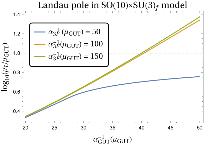
Figure 8: The scale $\mu_{L}$, measured in powers of $10$ above $\mu_{\rm GUT}$, when the Landau pole is reached. It is computed as a function of the value of the unified gauge coupling at the GUT scale $\alpha^{-1}_{\rm GUT}(\mu_{\rm GUT})$. The various lines show the cases with different starting values of the flavor gauge coupling $\alpha^{-1}_{3F}(\mu_{\rm GUT})$.

These coefficients lead to a Landau pole soon above the GUT scale, as shown in Fig. 8. For a typical value $\alpha^{-1}_{\rm GUT}(\mu_{\rm GUT})=40$ and a small flavor coupling (large $\alpha^{-1}_{3F}$), the Landau pole is reached within an order of magnitude from the GUT scale. The ${\rm SO}(10)$ scenario is thus borderline perturbative in this particular regime, but becomes non-perturbative as soon as unification happens with a larger value of the unified coupling (a smaller value of $\alpha^{-1}_{\rm GUT}(\mu_{\rm GUT})$).

Furthermore, notice that the one-loop beta coefficient for $\alpha^{-1}_{3F}$ is larger than for $\alpha^{-1}_{\rm GUT}$. Small values of the flavor coupling are now $\alpha^{-1}_{3F}(\mu_{\rm GUT})\geq 100$. At such values, the flavor coupling has little effect on the Landau pole, namely only through the two-loop off-diagonal coefficient. A value $\alpha^{-1}_{3F}(\mu_{\rm GUT})=50$ (blue curve), on the other hand, already corresponds to a large flavor coupling. The Landau pole is then reached much sooner and in the flavor coupling, again corresponding to a non-perturbative scenario.

References

- [1] L. Di Luzio, “Accidental SO(10) axion from gauged flavour,” JHEP 11 (2020) 074, arXiv:2008.09119 [hep-ph].
- [2] R. Peccei and H. R. Quinn, “CP Conservation in the Presence of Instantons,” Phys. Rev. Lett. 38 (1977) 1440–1443.
- [3] R. Peccei and H. R. Quinn, “Constraints Imposed by CP Conservation in the Presence of Instantons,” Phys. Rev. D 16 (1977) 1791–1797.
- [4] S. Weinberg, “A New Light Boson?,” Phys. Rev. Lett. 40 (1978) 223–226.
- [5] F. Wilczek, “Problem of Strong and Invariance in the Presence of Instantons,” Phys. Rev. Lett. 40 (1978) 279–282.
- [6] J. E. Kim, “Weak Interaction Singlet and Strong CP Invariance,” Phys. Rev. Lett. 43 (1979) 103.
- [7] M. A. Shifman, A. Vainshtein, and V. I. Zakharov, “Can Confinement Ensure Natural CP Invariance of Strong Interactions?,” Nucl. Phys. B 166 (1980) 493–506.
- [8] A. Zhitnitsky, “On Possible Suppression of the Axion Hadron Interactions. (In Russian),” Sov. J. Nucl. Phys. 31 (1980) 260.
- [9] M. Dine, W. Fischler, and M. Srednicki, “A Simple Solution to the Strong CP Problem with a Harmless Axion,” Phys. Lett. B 104 (1981) 199–202.
- [10] H. M. Georgi, L. J. Hall, and M. B. Wise, “Grand Unified Models With an Automatic Peccei-Quinn Symmetry,” Nucl. Phys. B 192 (1981) 409–416.
- [11] M. Dine and N. Seiberg, “String Theory and the Strong CP Problem,” Nucl. Phys. B 273 (1986) 109–124.
- [12] S. M. Barr and D. Seckel, “Planck scale corrections to axion models,” Phys. Rev. D 46 (1992) 539–549.
- [13] M. Kamionkowski and J. March-Russell, “Planck scale physics and the Peccei-Quinn mechanism,” Phys. Lett. B 282 (1992) 137–141, arXiv:hep-th/9202003.
- [14] R. Holman, S. D. Hsu, T. W. Kephart, E. W. Kolb, R. Watkins, and L. M. Widrow, “Solutions to the strong CP problem in a world with gravity,” Phys. Lett. B 282 (1992) 132–136, arXiv:hep-ph/9203206.
- [15] S. Ghigna, M. Lusignoli, and M. Roncadelli, “Instability of the invisible axion,” Phys. Lett. B 283 (1992) 278–281.
- [16] L. Randall, “Composite axion models and Planck scale physics,” Phys. Lett. B 284 (1992) 77–80.
- [17] B. A. Dobrescu, “The Strong CP problem versus Planck scale physics,” Phys. Rev. D 55 (1997) 5826–5833, arXiv:hep-ph/9609221.
- [18] K. S. Babu, I. Gogoladze, and K. Wang, “Stabilizing the axion by discrete gauge symmetries,” Phys. Lett. B 560 (2003) 214–222, arXiv:hep-ph/0212339.
- [19] M. Redi and R. Sato, “Composite Accidental Axions,” JHEP 05 (2016) 104, arXiv:1602.05427 [hep-ph].
- [20] H. Fukuda, M. Ibe, M. Suzuki, and T. T. Yanagida, “A ”gauged” Peccei–Quinn symmetry,” Phys. Lett. B 771 (2017) 327–331, arXiv:1703.01112 [hep-ph].
- [21] L. Di Luzio, E. Nardi, and L. Ubaldi, “Accidental Peccei-Quinn symmetry protected to arbitrary order,” Phys. Rev. Lett. 119 no. 1, (2017) 011801, arXiv:1704.01122 [hep-ph].
- [22] Q. Bonnefoy, E. Dudas, and S. Pokorski, “Axions in a highly protected gauge symmetry model,” Eur. Phys. J. C 79 no. 1, (2019) 31, arXiv:1804.01112 [hep-ph].
- [23] B. Lillard and T. M. P. Tait, “A High Quality Composite Axion,” JHEP 11 (2018) 199, arXiv:1811.03089 [hep-ph].
- [24] M. B. Gavela, M. Ibe, P. Quilez, and T. T. Yanagida, “Automatic Peccei–Quinn symmetry,” Eur. Phys. J. C 79 no. 6, (2019) 542, arXiv:1812.08174 [hep-ph].
- [25] M. Ardu, L. Di Luzio, G. Landini, A. Strumia, D. Teresi, and J.-W. Wang, “Axion quality from the (anti)symmetric of SU(N),” arXiv:2007.12663 [hep-ph].
- [26] R. Contino, A. Podo, and F. Revello, “Chiral models of composite axions and accidental Peccei-Quinn symmetry,” JHEP 04 (2022) 180, arXiv:2112.09635 [hep-ph].
- [27] Z. G. Berezhiani, “Horizontal Symmetry and Quark - Lepton Mass Spectrum: The SU(5) x SU(3)-h Model,” Phys. Lett. B 150 (1985) 177–181.
- [28] Z. G. Berezhiani and M. Y. Khlopov, “The Theory of broken gauge symmetry of families. (In Russian),” Sov. J. Nucl. Phys. 51 (1990) 739–746.
- [29] Z. G. Berezhiani, “The Weak Mixing Angles in Gauge Models with Horizontal Symmetry: A New Approach to Quark and Lepton Masses,” Phys. Lett. B 129 (1983) 99–102.
- [30] D. Chang and G. Senjanovic, “On Axion and Familons,” Phys. Lett. B188 (1987) 231.
- [31] D. Chang, P. B. Pal, and G. Senjanovic, “Axions From Chiral Family Symmetry,” Phys. Lett. B 153 (1985) 407–411.
- [32] L. Vecchi, “Axion quality straight from the GUT,” Eur. Phys. J. C 81 no. 10, (2021) 938, arXiv:2106.15224 [hep-ph].
- [33] K. S. Babu, B. Dutta, and R. N. Mohapatra, “Hybrid SO(10) Axion Model Without Quality Problem,” arXiv:2410.07323 [hep-ph].
- [34] L. Darmé and E. Nardi, “Exact accidental U(1) symmetries for the axion,” Phys. Rev. D 104 no. 5, (2021) 055013, arXiv:2102.05055 [hep-ph].
- [35] L. Darmé, E. Nardi, and C. Smarra, “The axion flavour connection,” JHEP 02 (2023) 201, arXiv:2211.05796 [hep-ph].
- [36] J. C. Pati and A. Salam, “Lepton Number as the Fourth Color,” Phys. Rev. D 10 (1974) 275–289. [Erratum: Phys.Rev.D 11, 703–703 (1975)].
- [37] S. Saad, “Fermion Masses and Mixings, Leptogenesis and Baryon Number Violation in Pati-Salam Model,” Nucl. Phys. B 943 (2019) 114630, arXiv:1712.04880 [hep-ph].
- [38] L. Di Luzio, “Pati-Salam Axion,” JHEP 07 (2020) 071, arXiv:2005.00012 [hep-ph].
- [39] A. Ernst, A. Ringwald, and C. Tamarit, “Axion Predictions in Models,” JHEP 02 (2018) 103, arXiv:1801.04906 [hep-ph].
- [40] L. Di Luzio, A. Ringwald, and C. Tamarit, “Axion mass prediction from minimal grand unification,” Phys. Rev. D 98 no. 9, (2018) 095011, arXiv:1807.09769 [hep-ph].
- [41] P. Fileviez Pérez, C. Murgui, and A. D. Plascencia, “Axion Dark Matter, Proton Decay and Unification,” JHEP 01 (2020) 091, arXiv:1911.05738 [hep-ph].
- [42] P. Fileviez Pérez, C. Murgui, and A. D. Plascencia, “The QCD Axion and Unification,” JHEP 11 (2019) 093, arXiv:1908.01772 [hep-ph].
- [43] Planck Collaboration, N. Aghanim et al., “Planck 2018 results. VI. Cosmological parameters,” Astron. Astrophys. 641 (2020) A6, arXiv:1807.06209 [astro-ph.CO]. [Erratum: Astron.Astrophys. 652, C4 (2021)].
- [44] R. Slansky, “Group Theory for Unified Model Building,” Phys. Rept. 79 (1981) 1–128.
- [45] R. N. Mohapatra and G. Senjanovic, “The Superlight Axion and Neutrino Masses,” Z. Phys. C 17 (1983) 53–56.
- [46] M. Srednicki, “Axion Couplings to Matter. 1. CP Conserving Parts,” Nucl. Phys. B 260 (1985) 689–700.
- [47] L. Di Luzio, M. Giannotti, E. Nardi, and L. Visinelli, “The landscape of QCD axion models,” Physics Reports 870 (2020) 1 – 117, arXiv:2003.01100 [hep-ph].
- [48] C. Abel et al., “Measurement of the Permanent Electric Dipole Moment of the Neutron,” Phys. Rev. Lett. 124 no. 8, (2020) 081803, arXiv:2001.11966 [hep-ex].
- [49] nEDM Collaboration, M. W. Ahmed et al., “A New Cryogenic Apparatus to Search for the Neutron Electric Dipole Moment,” JINST 14 no. 11, (2019) P11017, arXiv:1908.09937 [physics.ins-det].
- [50] n2EDM Collaboration, N. J. Ayres et al., “The design of the n2EDM experiment: nEDM Collaboration,” Eur. Phys. J. C 81 no. 6, (2021) 512, arXiv:2101.08730 [physics.ins-det].
- [51] J. Alexander et al., “The storage ring proton EDM experiment,” arXiv:2205.00830 [hep-ph].
- [52] R. M. Fonseca, “GroupMath: A Mathematica package for group theory calculations,” Comput. Phys. Commun. 267 (2021) 108085, arXiv:2011.01764 [hep-th].
- [53] M. van Leeuwen, A. M. Cohen, and B. Lisser, LiE, A Package for Lie Group Computations. Computer Algebra Nederland, Amsterdam, ISBN 90-74116-02-7, 1992.
- [54] L. Di Luzio, M. Fedele, M. Giannotti, F. Mescia, and E. Nardi, “Stellar evolution confronts axion models,” JCAP 02 no. 02, (2022) 035, arXiv:2109.10368 [hep-ph].
- [55] A. Caputo and G. Raffelt, “Astrophysical Axion Bounds: The 2024 Edition,” PoS COSMICWISPers (2024) 041, arXiv:2401.13728 [hep-ph].
- [56] P. Carenza, M. Giannotti, J. Isern, A. Mirizzi, and O. Straniero, “Axion Astrophysics,” arXiv:2411.02492 [hep-ph].
- [57] L. Di Luzio, V. Fiorentino, M. Giannotti, F. Mescia, and E. Nardi, “Do Finite Density Effects Jeopardize Axion Nucleophobia in Supernovae?,” arXiv:2410.04613 [hep-ph].
- [58] G. Grilli di Cortona, E. Hardy, J. Pardo Vega, and G. Villadoro, “The QCD axion, precisely,” JHEP 01 (2016) 034, arXiv:1511.02867 [hep-ph].
- [59] P. Carenza, T. Fischer, M. Giannotti, G. Guo, G. Martinez-Pinedo, and A. Mirizzi, “Improved axion emissivity from a supernova via nucleon-nucleon bremsstrahlung,” JCAP 1910 no. 10, (2019) 016, arXiv:1906.11844 [hep-ph].
- [60] P. Carenza, B. Fore, M. Giannotti, A. Mirizzi, and S. Reddy, “Enhanced Supernova Axion Emission and its Implications,” Phys. Rev. Lett. 126 no. 7, (2021) 071102, arXiv:2010.02943 [hep-ph].
- [61] F. Capozzi and G. Raffelt, “Axion and neutrino bounds improved with new calibrations of the tip of the red-giant branch using geometric distance determinations,” Phys. Rev. D 102 no. 8, (2020) 083007, arXiv:2007.03694 [astro-ph.SR].
- [62] O. Straniero, C. Pallanca, E. Dalessandro, I. Dominguez, F. R. Ferraro, M. Giannotti, A. Mirizzi, and L. Piersanti, “The RGB tip of galactic globular clusters and the revision of the axion-electron coupling bound,” Astron. Astrophys. 644 (2020) A166, arXiv:2010.03833 [astro-ph.SR].
- [63] M. M. Miller Bertolami, B. E. Melendez, L. G. Althaus, and J. Isern, “Revisiting the axion bounds from the Galactic white dwarf luminosity function,” JCAP 10 (2014) 069, arXiv:1406.7712 [hep-ph].
- [64] A. H. Córsico, L. G. Althaus, M. M. Miller Bertolami, and S. O. Kepler, “Pulsating white dwarfs: new insights,” Astron. Astrophys. Rev. 27 no. 1, (2019) 7, arXiv:1907.00115 [astro-ph.SR].
- [65] D. F. G. Fiorillo, M. Heinlein, H.-T. Janka, G. Raffelt, E. Vitagliano, and R. Bollig, “Supernova simulations confront SN 1987A neutrinos,” Phys. Rev. D 108 no. 8, (2023) 083040, arXiv:2308.01403 [astro-ph.HE].
- [66] K. Choi, S. H. Im, C. B. Park, and S. Yun, “Minimal Flavor Violation with Axion-like Particles,” JHEP 11 (2017) 070, arXiv:1708.00021 [hep-ph].
- [67] M. Chala, G. Guedes, M. Ramos, and J. Santiago, “Running in the ALPs,” Eur. Phys. J. C 81 no. 2, (2021) 181, arXiv:2012.09017 [hep-ph].
- [68] M. Bauer, M. Neubert, S. Renner, M. Schnubel, and A. Thamm, “The Low-Energy Effective Theory of Axions and ALPs,” JHEP 04 (2021) 063, arXiv:2012.12272 [hep-ph].
- [69] J. Bonilla, I. Brivio, M. B. Gavela, and V. Sanz, “One-loop corrections to ALP couplings,” JHEP 11 (2021) 168, arXiv:2107.11392 [hep-ph].
- [70] K. Choi, S. H. Im, H. J. Kim, and H. Seong, “Precision axion physics with running axion couplings,” JHEP 08 (2021) 058, arXiv:2106.05816 [hep-ph].
- [71] L. Di Luzio, F. Mescia, E. Nardi, and S. Okawa, “Renormalization group effects in astrophobic axion models,” Phys. Rev. D 106 no. 5, (2022) 055016, arXiv:2205.15326 [hep-ph].
- [72] L. Di Luzio, M. Giannotti, F. Mescia, E. Nardi, S. Okawa, and G. Piazza, “Running effects on QCD axion phenomenology,” Phys. Rev. D 108 no. 11, (2023) 115004, arXiv:2305.11958 [hep-ph].
- [73] D. J. E. Marsh, “Axion Cosmology,” Phys. Rept. 643 (2016) 1–79, arXiv:1510.07633 [astro-ph.CO].
- [74] C. A. J. O’Hare, “Cosmology of axion dark matter,” PoS COSMICWISPers (2024) 040, arXiv:2403.17697 [hep-ph].
- [75] M. Dine and W. Fischler, “The Not So Harmless Axion,” Phys. Lett. B 120 (1983) 137–141.
- [76] L. Abbott and P. Sikivie, “A Cosmological Bound on the Invisible Axion,” Phys. Lett. B 120 (1983) 133–136.
- [77] J. Preskill, M. B. Wise, and F. Wilczek, “Cosmology of the Invisible Axion,” Phys. Lett. B 120 (1983) 127–132.
- [78] M. Gorghetto, E. Hardy, and G. Villadoro, “More axions from strings,” SciPost Phys. 10 no. 2, (2021) 050, arXiv:2007.04990 [hep-ph].
- [79] M. Buschmann, J. W. Foster, A. Hook, A. Peterson, D. E. Willcox, W. Zhang, and B. R. Safdi, “Dark matter from axion strings with adaptive mesh refinement,” Nature Commun. 13 no. 1, (2022) 1049, arXiv:2108.05368 [hep-ph].
- [80] S. Borsanyi et al., “Calculation of the axion mass based on high-temperature lattice quantum chromodynamics,” Nature 539 no. 7627, (2016) 69–71, arXiv:1606.07494 [hep-lat].
- [81] M. Kawasaki, K. Saikawa, and T. Sekiguchi, “Axion dark matter from topological defects,” Phys. Rev. D 91 no. 6, (2015) 065014, arXiv:1412.0789 [hep-ph].
- [82] L. Di Luzio and P. Sørensen, “Axion production via trapped misalignment from Peccei-Quinn symmetry breaking,” JHEP 10 (2024) 239, arXiv:2408.04623 [hep-ph].
- [83] G. Lazarides and Q. Shafi, “Axion Models with No Domain Wall Problem,” Phys. Lett. 115B (1982) 21–25.
- [84] S. M. Barr, D. B. Reiss, and A. Zee, “Families, the Invisible Axion, and Domain Walls,” Phys. Lett. 116B (1982) 227–230.
- [85] P. Sikivie, “Of Axions, Domain Walls and the Early Universe,” Phys. Rev. Lett. 48 (1982) 1156–1159.
- [86] K. A. Beyer and S. Sarkar, “Ruling out light axions: The writing is on the wall,” SciPost Phys. 15 no. 1, (2023) 003, arXiv:2211.14635 [hep-ph].
- [87] Q. Lu, M. Reece, and Z. Sun, “The quality/cosmology tension for a post-inflation QCD axion,” JHEP 07 (2024) 227, arXiv:2312.07650 [hep-ph].
- [88] O. Wantz and E. Shellard, “Axion Cosmology Revisited,” Phys. Rev. D 82 (2010) 123508, arXiv:0910.1066 [astro-ph.CO].
- [89] C. O’Hare, “cajohare/axionlimits: Axionlimits.” https://cajohare.github.io/AxionLimits/, July, 2020.
- [90] S. De Panfilis, A. C. Melissinos, B. E. Moskowitz, J. T. Rogers, Y. K. Semertzidis, W. Wuensch, H. J. Halama, A. G. Prodell, W. B. Fowler, and F. A. Nezrick, “Limits on the Abundance and Coupling of Cosmic Axions at 4.5-Microev m(a) 5.0-Microev,” Phys. Rev. Lett. 59 (1987) 839.
- [91] W. Wuensch, S. De Panfilis-Wuensch, Y. K. Semertzidis, J. T. Rogers, A. C. Melissinos, H. J. Halama, B. E. Moskowitz, A. G. Prodell, W. B. Fowler, and F. A. Nezrick, “Results of a Laboratory Search for Cosmic Axions and Other Weakly Coupled Light Particles,” Phys. Rev. D 40 (1989) 3153.
- [92] CAST Collaboration, S. Andriamonje et al., “An Improved limit on the axion-photon coupling from the CAST experiment,” JCAP 04 (2007) 010, arXiv:hep-ex/0702006.
- [93] CAST Collaboration, V. Anastassopoulos et al., “New CAST Limit on the Axion-Photon Interaction,” Nature Phys. 13 (2017) 584–590, arXiv:1705.02290 [hep-ex].
- [94] B. T. McAllister, G. Flower, J. Kruger, E. N. Ivanov, M. Goryachev, J. Bourhill, and M. E. Tobar, “The ORGAN Experiment: An axion haloscope above 15 GHz,” Phys. Dark Univ. 18 (2017) 67–72, arXiv:1706.00209 [physics.ins-det].
- [95] M. Baryakhtar, J. Huang, and R. Lasenby, “Axion and hidden photon dark matter detection with multilayer optical haloscopes,” Phys. Rev. D 98 no. 3, (2018) 035006, arXiv:1803.11455 [hep-ph].
- [96] ADMX Collaboration, N. Du et al., “A Search for Invisible Axion Dark Matter with the Axion Dark Matter Experiment,” Phys. Rev. Lett. 120 no. 15, (2018) 151301, arXiv:1804.05750 [hep-ex].
- [97] D. Alesini et al., “Galactic axions search with a superconducting resonant cavity,” Phys. Rev. D 99 no. 10, (2019) 101101, arXiv:1903.06547 [physics.ins-det].
- [98] IAXO Collaboration, E. Armengaud et al., “Physics potential of the International Axion Observatory (IAXO),” JCAP 06 (2019) 047, arXiv:1904.09155 [hep-ph].
- [99] M. Lawson, A. J. Millar, M. Pancaldi, E. Vitagliano, and F. Wilczek, “Tunable axion plasma haloscopes,” Phys. Rev. Lett. 123 no. 14, (2019) 141802, arXiv:1904.11872 [hep-ph].
- [100] N. Crisosto, P. Sikivie, N. S. Sullivan, D. B. Tanner, J. Yang, and G. Rybka, “ADMX SLIC: Results from a Superconducting Circuit Investigating Cold Axions,” Phys. Rev. Lett. 124 no. 24, (2020) 241101, arXiv:1911.05772 [astro-ph.CO].
- [101] HAYSTAC Collaboration, K. M. Backes et al., “A quantum-enhanced search for dark matter axions,” Nature 590 no. 7845, (2021) 238–242, arXiv:2008.01853 [quant-ph].
- [102] M. D. Ortiz et al., “Design of the ALPS II optical system,” Phys. Dark Univ. 35 (2022) 100968, arXiv:2009.14294 [physics.optics].
- [103] D. Alesini et al., “Search for invisible axion dark matter of mass meV with the QUAX– experiment,” Phys. Rev. D 103 no. 10, (2021) 102004, arXiv:2012.09498 [hep-ex].
- [104] J. Schütte-Engel, D. J. E. Marsh, A. J. Millar, A. Sekine, F. Chadha-Day, S. Hoof, M. N. Ali, K.-C. Fong, E. Hardy, and L. Šmejkal, “Axion quasiparticles for axion dark matter detection,” JCAP 08 (2021) 066, arXiv:2102.05366 [hep-ph].
- [105] CAST Collaboration, A. A. Melcón et al., “First results of the CAST-RADES haloscope search for axions at 34.67 eV,” JHEP 21 (2020) 075, arXiv:2104.13798 [hep-ex].
- [106] ADMX Collaboration, C. Bartram et al., “Search for Invisible Axion Dark Matter in the 3.3–4.2 eV Mass Range,” Phys. Rev. Lett. 127 no. 26, (2021) 261803, arXiv:2110.06096 [hep-ex].
- [107] T. Grenet, R. Ballou, Q. Basto, K. Martineau, P. Perrier, P. Pugnat, J. Quevillon, N. Roch, and C. Smith, “The Grenoble Axion Haloscope platform (GrAHal): development plan and first results,” arXiv:2110.14406 [hep-ex].
- [108] Z. Zhang, D. Horns, and O. Ghosh, “Search for dark matter with an LC circuit,” Phys. Rev. D 106 no. 2, (2022) 023003, arXiv:2111.04541 [hep-ex].
- [109] BREAD Collaboration, J. Liu et al., “Broadband Solenoidal Haloscope for Terahertz Axion Detection,” Phys. Rev. Lett. 128 no. 13, (2022) 131801, arXiv:2111.12103 [physics.ins-det].
- [110] J. W. Foster, S. J. Witte, M. Lawson, T. Linden, V. Gajjar, C. Weniger, and B. R. Safdi, “Extraterrestrial Axion Search with the Breakthrough Listen Galactic Center Survey,” Phys. Rev. Lett. 129 no. 25, (2022) 251102, arXiv:2202.08274 [astro-ph.CO].
- [111] DMRadio Collaboration, L. Brouwer et al., “Projected sensitivity of DMRadio-m3: A search for the QCD axion below 1 eV,” Phys. Rev. D 106 no. 10, (2022) 103008, arXiv:2204.13781 [hep-ex].
- [112] D. Alesini et al., “Search for Galactic axions with a high-Q dielectric cavity,” Phys. Rev. D 106 no. 5, (2022) 052007, arXiv:2208.12670 [hep-ex].
- [113] A. K. Yi et al., “Axion Dark Matter Search around 4.55 eV with Dine-Fischler-Srednicki-Zhitnitskii Sensitivity,” Phys. Rev. Lett. 130 no. 7, (2023) 071002, arXiv:2210.10961 [hep-ex].
- [114] HAYSTAC Collaboration, M. J. Jewell et al., “New results from HAYSTAC’s phase II operation with a squeezed state receiver,” Phys. Rev. D 107 no. 7, (2023) 072007, arXiv:2301.09721 [hep-ex].
- [115] DALI Collaboration, J. De Miguel, J. F. Hernández-Cabrera, E. Hernández-Suárez, E. Joven-Álvarez, C. Otani, and J. A. Rubiño Martín, “Discovery prospects with the Dark-photons & Axion-like particles Interferometer,” Phys. Rev. D 109 no. 6, (2024) 062002, arXiv:2303.03997 [hep-ph].
- [116] D. Alesini et al., “The future search for low-frequency axions and new physics with the FLASH resonant cavity experiment at Frascati National Laboratories,” Phys. Dark Univ. 42 (2023) 101370, arXiv:2309.00351 [physics.ins-det].
- [117] CAPP Collaboration, S. Ahn et al., “Extensive Search for Axion Dark Matter over 1 GHz with CAPP’S Main Axion Experiment,” Phys. Rev. X 14 no. 3, (2024) 031023, arXiv:2402.12892 [hep-ex].
- [118] A. P. Quiskamp, G. Flower, S. Samuels, B. T. McAllister, P. Altin, E. N. Ivanov, M. Goryachev, and M. E. Tobar, “Near-quantum limited axion dark matter search with the ORGAN experiment around 26 eV,” arXiv:2407.18586 [hep-ex].
- [119] ADMX Collaboration, C. Bartram et al., “Axion Dark Matter eXperiment around 3.3 eV with Dine-Fischler-Srednicki-Zhitnitsky Discovery Ability,” arXiv:2408.15227 [hep-ex].
- [120] B. A. d. S. Garcia et al., “First search for axion dark matter with a Madmax prototype,” arXiv:2409.11777 [hep-ex].
- [121] L. J. Hall, K. Jedamzik, J. March-Russell, and S. M. West, “Freeze-In Production of FIMP Dark Matter,” JHEP 03 (2010) 080, arXiv:0911.1120 [hep-ph].
- [122] J. Heeck, “Unbroken B – L symmetry,” Phys. Lett. B 739 (2014) 256–262, arXiv:1408.6845 [hep-ph].
- [123] M. Kawasaki, K. Kohri, and N. Sugiyama, “MeV scale reheating temperature and thermalization of neutrino background,” Phys. Rev. D 62 (2000) 023506, arXiv:astro-ph/0002127.
- [124] S. Hannestad, “What is the lowest possible reheating temperature?,” Phys. Rev. D 70 (2004) 043506, arXiv:astro-ph/0403291.
- [125] F. De Bernardis, L. Pagano, and A. Melchiorri, “New constraints on the reheating temperature of the universe after WMAP-5,” Astropart. Phys. 30 (2008) 192–195.
- [126] A. Strumia and F. Vissani, “Neutrino masses and mixings and…,” arXiv:hep-ph/0606054.
- [127] S. Hannestad, I. Tamborra, and T. Tram, “Thermalisation of light sterile neutrinos in the early universe,” JCAP 07 (2012) 025, arXiv:1204.5861 [astro-ph.CO].
- [128] B. Dasgupta and J. Kopp, “Sterile Neutrinos,” Phys. Rept. 928 (2021) 1–63, arXiv:2106.05913 [hep-ph].
- [129] S. Dodelson and L. M. Widrow, “Sterile-neutrinos as dark matter,” Phys. Rev. Lett. 72 (1994) 17–20, arXiv:hep-ph/9303287.
- [130] A. Boyarsky, O. Ruchayskiy, and M. Shaposhnikov, “The Role of sterile neutrinos in cosmology and astrophysics,” Ann. Rev. Nucl. Part. Sci. 59 (2009) 191–214, arXiv:0901.0011 [hep-ph].
- [131] J. Lesgourgues and S. Pastor, “Neutrino mass from Cosmology,” Adv. High Energy Phys. 2012 (2012) 608515, arXiv:1212.6154 [hep-ph].
- [132] M. Drewes et al., “A White Paper on keV Sterile Neutrino Dark Matter,” JCAP 01 (2017) 025, arXiv:1602.04816 [hep-ph].
- [133] K. N. Abazajian, “Sterile neutrinos in cosmology,” Phys. Rept. 711-712 (2017) 1–28, arXiv:1705.01837 [hep-ph].
- [134] S. Gariazzo, P. F. de Salas, and S. Pastor, “Thermalisation of sterile neutrinos in the early Universe in the 3+1 scheme with full mixing matrix,” JCAP 07 (2019) 014, arXiv:1905.11290 [astro-ph.CO].
- [135] M. Cirelli, A. Strumia, and J. Zupan, “Dark Matter,” arXiv:2406.01705 [hep-ph].
- [136] D. Nötzold and G. Raffelt, “Neutrino dispersion at finite temperature and density,” Nucl. Phys. B 307 (1988) 924–936.
- [137] ATLAS Collaboration, G. Aad et al., “Combination of searches for invisible decays of the Higgs boson using 139 fb1 of proton-proton collision data at s=13 TeV collected with the ATLAS experiment,” Phys. Lett. B 842 (2023) 137963, arXiv:2301.10731 [hep-ex].
- [138] R. An, V. Gluscevic, E. O. Nadler, and Y. Zhang, “Can Neutrino Self-interactions Save Sterile Neutrino Dark Matter?,” Astrophys. J. Lett. 954 no. 1, (2023) L18, arXiv:2301.08299 [astro-ph.CO].
- [139] S. Tremaine and J. E. Gunn, “Dynamical Role of Light Neutral Leptons in Cosmology,” Phys. Rev. Lett. 42 (1979) 407–410.
- [140] J. Alvey, N. Sabti, V. Tiki, D. Blas, K. Bondarenko, A. Boyarsky, M. Escudero, M. Fairbairn, M. Orkney, and J. I. Read, “New constraints on the mass of fermionic dark matter from dwarf spheroidal galaxies,” Mon. Not. Roy. Astron. Soc. 501 no. 1, (2021) 1188–1201, arXiv:2010.03572 [hep-ph].
- [141] Particle Data Group Collaboration, R. L. Workman et al., “Review of Particle Physics,” PTEP 2022 (2022) 083C01.
- [142] Simons Observatory Collaboration, M. H. Abitbol et al., “The Simons Observatory: Astro2020 Decadal Project Whitepaper,” Bull. Am. Astron. Soc. 51 (2019) 147, arXiv:1907.08284 [astro-ph.IM].
- [143] Simons Observatory Collaboration, P. Ade et al., “The Simons Observatory: Science goals and forecasts,” JCAP 02 (2019) 056, arXiv:1808.07445 [astro-ph.CO].
- [144] EUCLID Collaboration, R. Laureijs et al., “Euclid Definition Study Report,” arXiv:1110.3193 [astro-ph.CO].
- [145] CMB-HD Collaboration, S. Aiola et al., “Snowmass2021 CMB-HD White Paper,” arXiv:2203.05728 [astro-ph.CO].
- [146] S.-P. Li and X.-J. Xu, “Neff constraints on light mediators coupled to neutrinos: the dilution-resistant effect,” JHEP 10 (2023) 012, arXiv:2307.13967 [hep-ph].
- [147] F. D’Eramo, F. Hajkarim, and A. Lenoci, “Dark radiation from the primordial thermal bath in momentum space,” JCAP 03 (2024) 009, arXiv:2311.04974 [hep-ph].
- [148] F. D’Eramo, F. Hajkarim, and S. Yun, “Thermal QCD Axions across Thresholds,” JHEP 10 (2021) 224, arXiv:2108.05371 [hep-ph].
- [149] L. Caloni, P. Stengel, M. Lattanzi, and M. Gerbino, “Constraining UV freeze-in of light relics with current and next-generation CMB observations,” arXiv:2405.09449 [astro-ph.CO].
- [150] M. Badziak, K. Harigaya, M. Łukawski, and R. Ziegler, “Thermal production of astrophobic axions,” JHEP 09 (2024) 136, arXiv:2403.05621 [hep-ph].
- [151] M. Berbig, “Freeze-In of radiative keV-scale neutrino dark matter from a new U(1)B-L,” JHEP 09 (2022) 101, arXiv:2203.04276 [hep-ph].
- [152] S. Chang and K. Choi, “Hadronic axion window and the big bang nucleosynthesis,” Phys. Lett. B 316 (1993) 51–56, arXiv:hep-ph/9306216.
- [153] S. Hannestad, A. Mirizzi, and G. Raffelt, “New cosmological mass limit on thermal relic axions,” JCAP 07 (2005) 002, arXiv:hep-ph/0504059.
- [154] L. Di Luzio, G. Martinelli, and G. Piazza, “Breakdown of chiral perturbation theory for the axion hot dark matter bound,” Phys. Rev. Lett. 126 no. 24, (2021) 241801, arXiv:2101.10330 [hep-ph].
- [155] A. Notari, F. Rompineve, and G. Villadoro, “Improved Hot Dark Matter Bound on the QCD Axion,” Phys. Rev. Lett. 131 no. 1, (2023) 011004, arXiv:2211.03799 [hep-ph].
- [156] L. Di Luzio, J. Martin Camalich, G. Martinelli, J. A. Oller, and G. Piazza, “Axion-pion thermalization rate in unitarized NLO chiral perturbation theory,” Phys. Rev. D 108 no. 3, (2023) 035025, arXiv:2211.05073 [hep-ph].
- [157] F. Bianchini, G. G. di Cortona, and M. Valli, “QCD axion: Some like it hot,” Phys. Rev. D 110 no. 12, (2024) 123527, arXiv:2310.08169 [hep-ph].
- [158] S. Bertolini, L. Di Luzio, and F. Nesti, “Axion-mediated forces, CP violation and left-right interactions,” Phys. Rev. Lett. 126 no. 8, (2021) 081801, arXiv:2006.12508 [hep-ph].
- [159] R. Feger and T. W. Kephart, “LieART—A Mathematica application for Lie algebras and representation theory,” Comput. Phys. Commun. 192 (2015) 166–195, arXiv:1206.6379 [math-ph].
- [160] R. Feger, T. W. Kephart, and R. J. Saskowski, “LieART 2.0 – A Mathematica application for Lie Algebras and Representation Theory,” Comput. Phys. Commun. 257 (2020) 107490, arXiv:1912.10969 [hep-th].
- [161] S. A. R. Ellis and J. D. Wells, “Visualizing gauge unification with high-scale thresholds,” Phys. Rev. D 91 no. 7, (2015) 075016, arXiv:1502.01362 [hep-ph].
- [162] S. Bertolini, L. Di Luzio, and M. Malinsky, “Intermediate mass scales in the non-supersymmetric SO(10) grand unification: A Reappraisal,” Phys. Rev. D 80 (2009) 015013, arXiv:0903.4049 [hep-ph].
- [163] D. R. T. Jones, “The Two Loop beta Function for a G(1) x G(2) Gauge Theory,” Phys. Rev. D 25 (1982) 581.
- [164] W. J. Marciano, “Quantitative tests of the standard model of electroweak interactions,” Ann. Rev. Nucl. Part. Sci. 41 (1991) 469–509.
- [165] J. H. Kuhn and M. Steinhauser, “A Theory driven analysis of the effective QED coupling at M(Z),” Phys. Lett. B 437 (1998) 425–431, arXiv:hep-ph/9802241.
- [166] W. Martens, L. Mihaila, J. Salomon, and M. Steinhauser, “Minimal Supersymmetric SU(5) and Gauge Coupling Unification at Three Loops,” Phys. Rev. D 82 (2010) 095013, arXiv:1008.3070 [hep-ph].
- [167] C. Sturm, “Leptonic contributions to the effective electromagnetic coupling at four-loop order in QED,” Nucl. Phys. B 874 (2013) 698–719, arXiv:1305.0581 [hep-ph].
- [168] Particle Data Group Collaboration, P. A. Zyla et al., “Review of Particle Physics,” PTEP 2020 no. 8, (2020) 083C01.
- [169] S. Bertolini, L. Di Luzio, and M. Malinsky, “On the vacuum of the minimal nonsupersymmetric SO(10) unification,” Phys. Rev. D 81 (2010) 035015, arXiv:0912.1796 [hep-ph].
- [170] S. Bertolini, L. Di Luzio, and M. Malinsky, “Seesaw Scale in the Minimal Renormalizable SO(10) Grand Unification,” Phys. Rev. D 85 (2012) 095014, arXiv:1202.0807 [hep-ph].
- [171] S. Bertolini, L. Di Luzio, and M. Malinsky, “Light color octet scalars in the minimal SO(10) grand unification,” Phys. Rev. D 87 no. 8, (2013) 085020, arXiv:1302.3401 [hep-ph].
- [172] L. Graf, M. Malinsky, T. Mede, and V. Susic, “One-loop pseudo-Goldstone masses in the minimal Higgs model,” Phys. Rev. D 95 no. 7, (2017) 075007, arXiv:1611.01021 [hep-ph].
- [173] K. Jarkovská, M. Malinský, T. Mede, and V. Susič, “Quantum nature of the minimal potentially realistic SO(10) Higgs model,” Phys. Rev. D 105 no. 9, (2022) 095003, arXiv:2109.06784 [hep-ph].
- [174] K. Jarkovská, M. Malinský, and V. Susič, “Trouble with the minimal renormalizable SO(10) GUT,” Phys. Rev. D 108 no. 5, (2023) 055003, arXiv:2304.14227 [hep-ph].