Turing Instability Suppressed and Induced by Multiplicative Noise in Brusselator System
Abstract
The effect of multiplicative noise to the Turing instability of the Brusselator system is investigated. We show that when the noise acts on both of the concentrations with the same intensities, then the Turing instability is suppressed provided that the intensities are sufficiently large. This aligns with the stabilizing effect of multiplicative noise in partial differential equations. Utilizing the linearized system, we can quantify the magnitude of noise which stabilizes the system. On the other hand, when the noise is involving only one concentration, then the Turing instability can be triggered with suitable intensities. These are confirmed by numerical simulations.
Keywords: Brusselator system; Turing instability; Multiplicative noise; Instability induced/suppressed by noise.
1 Introduction
Reaction-diffusion system (RDS) provides a compelling and useful modeling tool for many problems in real life. One of the main reasons is that, even a simple RDS can exhibit many complex patterns as shown in the well known work [Pea93]. Revealing the mechanism for the formation of these patterns is the objective of many works since then or even earlier. One prime example is the famous work of Turing [Tur52] where he argued that one possible mechanism is the complicated interplay between diffusion and (chemical) reactions in terms of activators and inhibitors. More precisely, it was shown that if the activator has short range diffusion and inhibitor has long range diffusion, then the stable spatially homogeneous equilibrium becomes unstable, consequently leading to spatially inhomogeneous patterns. This has initiated a now classical topic named Turing instability, and is the subject of a vast number of research works (see refer the interested reader to the book [Mur07] for more details).
The Turing instability has been confirmed in certain real life biological systems, see for instance [MOK10] where experiments on zebrafish stripes showed that they are formed as an interaction of two types of cells, playing roles of activator and inhibitor, following Turing mechanism. However, the different scales of diffusion might not be “physical” in biological systems cf. [HG21], so researchers looked for additional features that suppress or trigger Turing instability, including systems in time evolving domains [MGM10, VGKK21], systems with spatially inhomogeneous coefficients [VG21, KGK19], or the effect of random noise. For instance, at the level of reaction-diffusion master equations, [HH12] showed that noise can induce spatial patterns for chemical reactions, and [DMPT18] studied the effects of noise on patterns for RDS or population dynamics. Some existing works looked at the effect of additive noise, for instance, [KBR24] showed induced pattern for thermochemical kinetics, [BJG17] investigated giant amplification of noise in fluctuation-induced pattern formation, and [BKR21] considered the sensitivity of Turing patterns. For multiplicative noise, [ZWSI17] used some explicit stochastic noises and Taylor expansion to obtain their effect on Turing bifurcation, while [XGAS23] investigated the effects of noise on critical points of Turing instability on networks. Stochastic Turing patterns triggered by noise have been even confirmed through experiments in [KML+18].
For scalar PDE, multiplicative noise has been known to have stabilizing effect, see e.g. [Kwi99, CLM01, CKS06, CCLR07]. Especially, in [Kwi99], by looking at the Fourier analysis of a linear PDE, it was shown that the stabilization is because the multiplicative noise shifts the spectral of the Laplacian to the left with the magnitude proportional to the (square of) noise intensities. In a way, this could be seen as scaling of the range of diffusion. For systems, it is therefore natural to ask: what happens if the scaling for different species are the same or different? In this paper, we investigate this question by looking at the PDE Brusselator system with multiplicative noise. It will be demonstrated that, if the noise intensities are the same for different species, multiplicative noise has suppression effect on Turing instability. On the other hand, if the noise is acting on only one species, it could induce instability even if the short range activator - long range inhibitor is not fulfilled for deterministic systems. The suppression effects are proved by analyzing a linearized systems and using some Fourier analysis, while the induced instability is shown via numerical simulations. It is remarked that the analysis can be carried out for other RDS concerning Turing instability. We would like to also point out several works studying the effect of noise in Brusselator system in different contexts, see e.g. [YBJK97, BR00, EOM24] and references therein.
2 Stochastic Brusselator system
The Brusselator is characterized by the reactions
for certain chemicals and . It is assumed that are in large excess, and therefore their concentrations can be taken as constants, say and . We arrive at the following reaction-diffusion system for the concentrations of and , which are denoted by and , respectively,
| (1) |
where are positive diffusion coefficients. Here , , is an open, bounded domain with smooth boundary (in case ), and is the outward normal vector at . Due to the homogeneous Neumann boundary conditions, it is straightforward to see that is the unique spatially homogeneous steady state of (1). Moreover, if , this steady state is asymptotically stable. It is also well-known, see e.g. [Per15] that in this case, Turing instability occurs when , leading to the formation of patterns, while the steady state is still asymptotically stable when . In this work, we are interested in the effect of multiplicative noise concerning this Turing instability. More precisely, we consider the following stochastic Brusselator system with multiplicative noise
| (2) |
where is a real-valued Wiener process, and are noise intensities. The forms of the noise are so that is also a steady state of the stochastic system.
3 Linear stability analysis for the stochastic system
The linearized system of (2) around the equilibrium reads as
| (3) |
Denoting and , we rewrite the linearized system in the general form
| (4) |
For simplicity, we consider the case where is the activator and is the inhibitor, meaning that and , which consequently imposes . In this case, it is well-known that, if is sufficiently small, then Turing instability occurs (see e.g. [Per15, Theorem 7.1]).
First we have a look at the corresponding deterministic differential system reads as
| (5) |
Due to the condition , it follows that
Therefore, the zero solution to the ODE system (5) is exponentially stable, i.e. there exist constants such that
To analyze the stochastic system, we consider the eigenvalue problem with Neumann boundary condition
It is well-known that there is a system of eigenvalue-eigenfunction such that
-
•
,
-
•
is an orthonormal basis of .
We use the same basic decomposition technique for and , i.e.,
| (6) |
Inserting these into system (4) then multiply by and integrate over , we get
| (7) |
By defining
we arrive to the following stochastic differential system for each
| (8) |
In the following subsections, we analyze the case of same noise intensities and different intensities separately.
3.1 The case of the same noise intensities
If , then and are commutative and we have the formal solution to (8) (see e.g. [Mao07, Section 3.4]) as
| (9) |
Where with and . We now investigate the eigenvalues of .
Lemma 3.1
There exists and such that for all
where denotes the spectrum of a matrix .
Proof:
Denote by . The characteristic polynomial of is
The eigenvalues and of satisfy
| (10) |
Since and , we have for all and all . We first rewrite as
and deduce that, thanks to and , there exists such that
It follows then from (10) that and . If , then
If , then are both negative and
provided . Therefore, we can choose such that , then for all and for any ,
with
Theorem 3.2
Assume that . Then for any diffusion coefficients , the solution to the linearized Brusselator system (3) is exponentially converging to zero as almost surely, provided . Moreover, we have the Lyapunov exponent
with
Proof:
From (6), Parseval’s identity and (9) it follows that
Thanks to the property of white noise, we have
and therefore, for any there exists such that
almost surely. Therefore,
On the other hand, from Lemma 3.1,
Thus we can estimate
almost surely for arbitrary. This confirms the Lyapunov exponent and finishes the proof of Theorem 3.2.
Theorem 3.2 shows that with sufficiently large noise intensities, system (3) is stable regardless of diffusion coefficients. A direct consequence is the suppression of Turing instability by noise. This is demonstrated in Figures 1 and 2 where we consider the one dimensional case . More precisely, Figure 1 shows the evolution of solutions to (3) when Turing instability occurs. The parameters in this case
satisfy , which makes the ODE (5) stable, but since is sufficiently small, the PDE system (3) is unstable. From initial data being small perturbation of the equilibrium , the solutions eventually grow to have spatially inhomogeneous profiles, which are shown in Figures 1(a) and 1(b). The evolution of the norm in Figure 1(c) shows that, this instability happens after an initial decay phase on the time interval , and after that the norms of solutions grow exponentially. Moreover, a closer inspection in Figure 1(d) shows that there are only a finite number of eigenmodes in the middle (between and ) which are unstable, while the others stay stable. This can be also shown theoretically (see e.g. [Per15]).
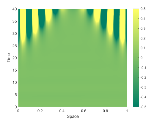
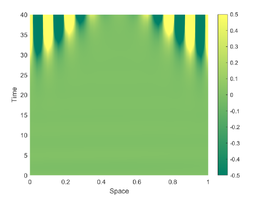
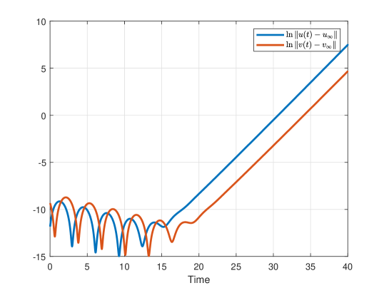
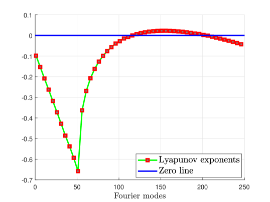
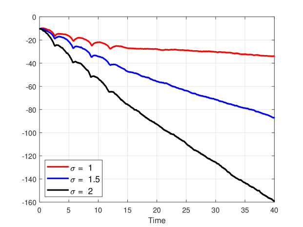
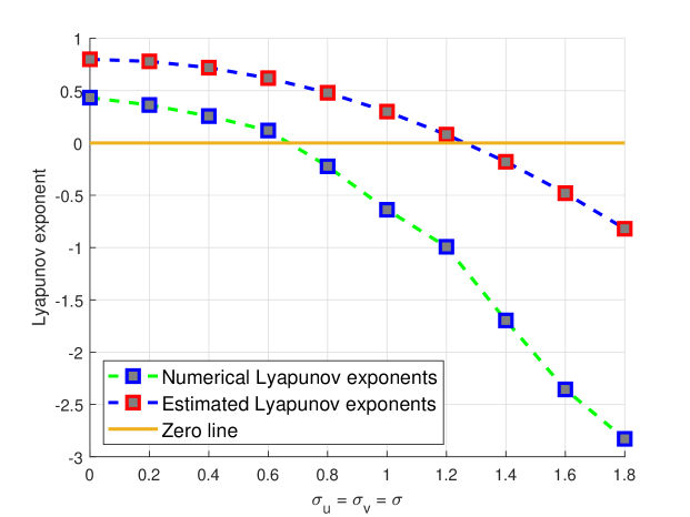
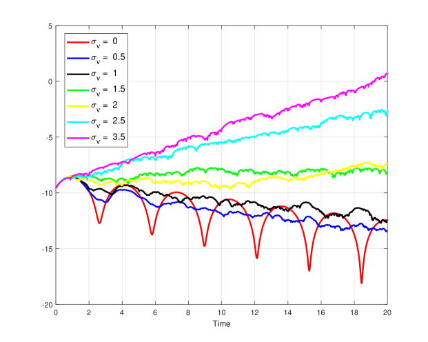
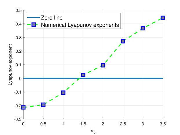
Figure 2 shows the suppression of this instability by sufficiently large noise intensities, which are the same for the equations of and , i.e. . In Figure 2(a), we see behaves almost linearly with negative slopes, which means that the solutions decay to zero exponentially. Moreover, the bigger the noise intensities , the faster solutions converge to zero, which is consistent with Theorem 3.2 where the Lyapunov exponent decreases for increasing . Figure 2(b) demonstrates the behavior of Lyapunov exponents according to the noise intensity . The green curve with blue points shows the real Lapunov exponent, which becomes negative when is somewhere in between and , and decreases further as grows, while the blue curve with red points shows an upper bound of the Lyapunov exponent established in Theorem 3.2. It can be seen that, while being qualitatively accurate, these upper bounds are far from being sharp. Showing optimal bound of Lyapunov exponent for (3) depending on is left for future investigation.
Since (3) is linear, the stability, in the presence of noise, is in fact global. This is demonstrated in Figure 3, where the solutions converge to zero with initial data being far away from the equilibrium .

3.2 The case of different noise intensities
In this part, the noise intensities for and are different. For the sake of simplicity, we fix and vary . Due to this difference, the matrix and in (8) are generally no longer commutative, and consequently an explicit expression of solutions similarly to (9) is not possible. Furthermore, due to the degeneracy of , the stabilization and destabilization theory in e.g. [Mao07, Chapter 4] cannot be applied to determine the stability of (8). Here, we show by numerical simulations that this difference in noise intensities destabilizes the system (8), and consequently the linear PDE system (3).
Consider and the set of parameters
which make the ODE system (5) stable since . Moreover, since is large, the PDE system is also stable, i.e. no Turing instability occurs. The destabilization by noise with and is shown in Figure 4, where part (a) shows the evolution of for different values of . Here we see that starting from , the solution starts to grow exponentially. This is confirmed in Figure 4(b), where numerical Lyapunov exponents are shown. From this figure, the Lyapunov exponent is monotone increasing in the value of , and starting from , the Lyapunov exponent becomes positive.
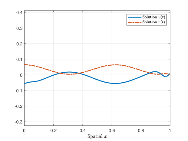
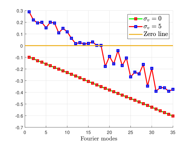
To analyze it further, we plot the profiles of solution at final time Figure 5(a), where it clearly shows that the solution becomes spatially inhomogeneous. Moreover, in Figure 5(b), we compute the Lyapunov exponents for different eigenmodes. The green line with red markers present the Lypanov exponents of the linearized system without noise, which shows that all these exponents are negative, causing the exponential stability of the system. In the presence of noise (while ), the Lyapunov exponents of different modes, presented by the red line with blue markers, show that some first modes (from to ) become positive, leading to the instability of the stochastic system. Unlike the case of deterministic instability in Figure 1(d), the unstable modes seem to always contain the first eigenmodes.
4 Numerical Simulations for Nonlinear Systems
In this section, we investigate the effect of noise to the stability of nonlinear system (1) through numerical simulations. The theoretical investigation is beyond the scope of this paper and is therefore left for future studies.
4.1 Turing instability prevented by noise
We consider and the following parameters
the time horizon , and the discretization and . The initial data is set to be
where and are random numbers between and .
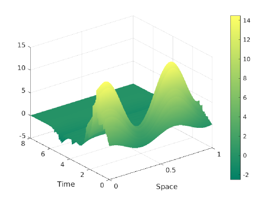
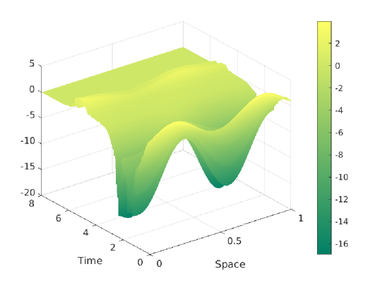
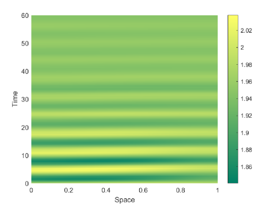
The deterministic case . In this case, the Turing condition is satisfied and therefore, the deterministic system possesses Turing instability, see Figure 6. In this case, we can see from Figures 6(a) and 6(b) that the solution converges to a stable spatially inhomogeneous steady state, which is depicted in Figure 6(d).
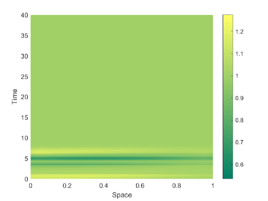
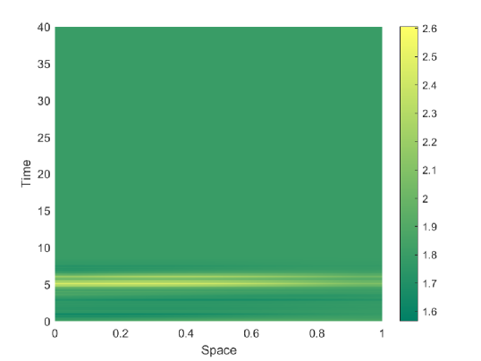
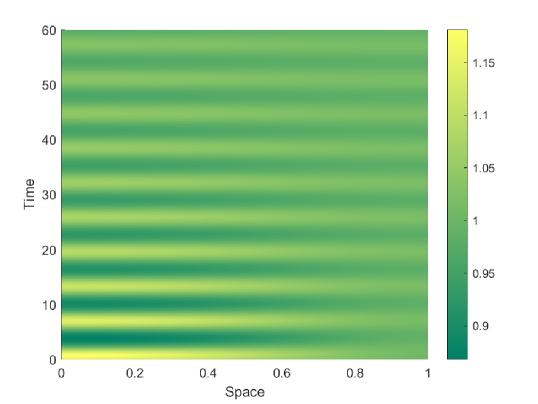
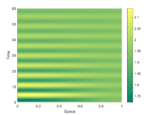
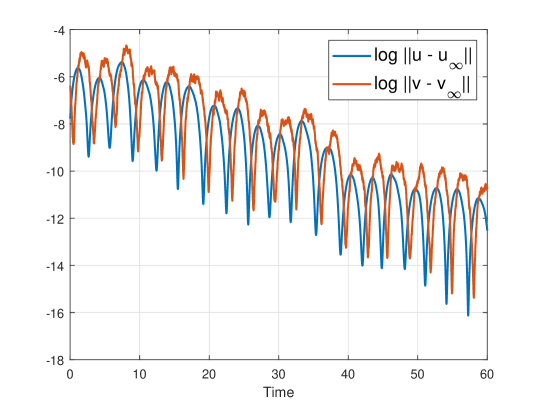
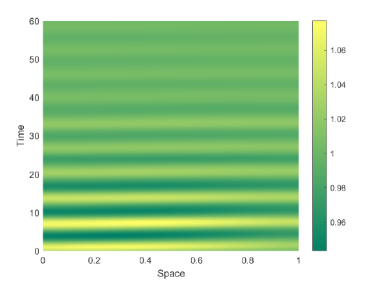
The case of the same noise intensities . In this case, the suppression of Turing instability is proved theoretically for the linearized system in the previous section. Here, numerical simulation suggests that it is also true for the nonlinear regime. Figure 7(a) shows that the solution decays exponentially to the equilibrium . The evolution of and are shown in Figures in 7(b) and 7(c).
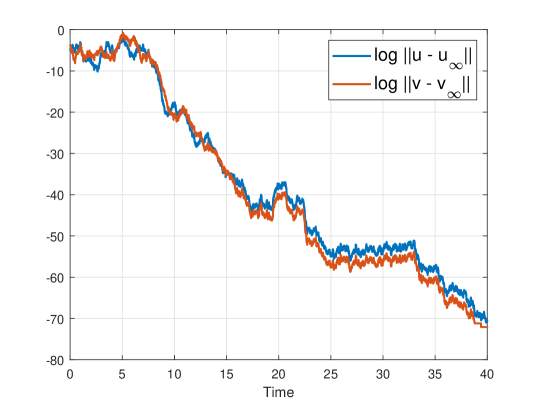
4.2 Turing instability induced by noise
We consider the following parameters
the time horizon , and the descretization and .
The deterministic case . In this case, the Turing condition is not satisfied as is not sufficiently small (see e.g. [Per15, Chapter 7], and therefore we have the convergence towards the equilibrium and , see Figure 8.
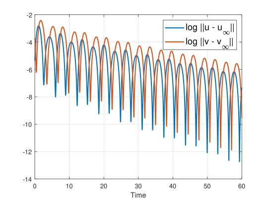
The case with small noise intensities and . For small noise, the stability of the system is still in effect, see Figure 9. Similar to the linearized case, for small magnitude of , the disturbance of noise is not sufficient to drive the system away from the stable regime. The solution still converges exponentially to equilibrium, with some disruption, as shown in Figure 9. This can be compared with Figure 4(b), where with small magnitude of the Lyapunov exponent is still negative, meaning that linearized system, and consequently the nonlinear system, is still stable.
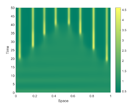
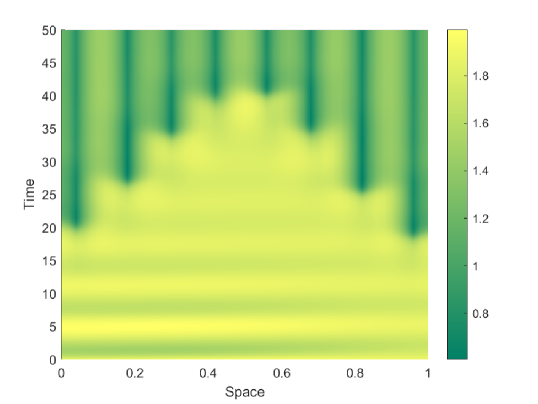
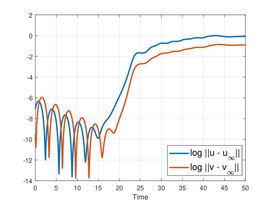
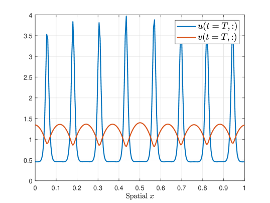
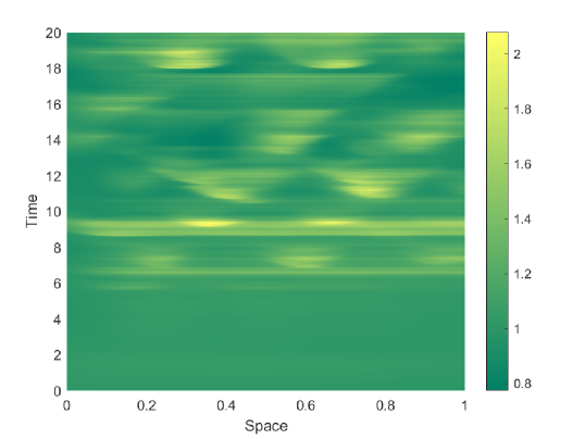
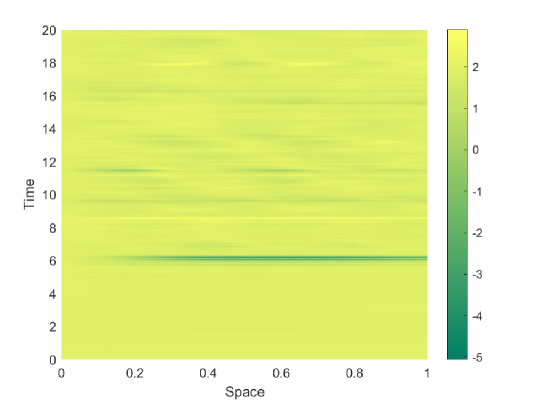
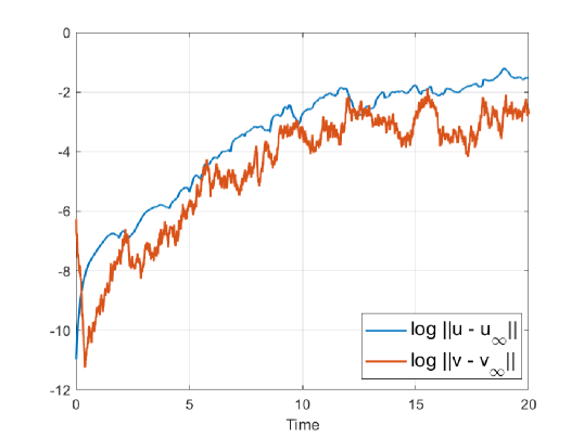
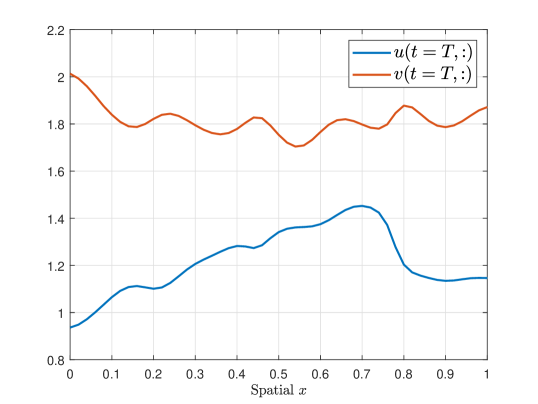
The case with bigger noise intensities and . Finally, when the noise intensity is sufficiently large, the noise destabilizes the system as shown in Figure 10. The solution is no longer converging to the spatially homogeneous steady state . However, unlike the case of deterministic instability, due to the random noise, the solution also does not converge to a stable spatially inhomogeneous steady state, but fluctuates with different profiles. The large time behavior of solution in this case remains open, even in the numerical simulation.
5 Conclusion and Future Work
In this work, we have demonstrated that a multiplicative noise in Brusselator can have suppression or induced effect on Turing instability. More precisely, when both the noise intensities on both species are the same, then the Turing instability is suppressed if the intensities are sufficiently large. This is also theoretically proved by analyzing the linearized system around equilibrium, and using explicit expression of solutions to SDE systems when the deterministic and stochastic parts are commutative. On the other hand, when one noise intensity is zero, multiplicative noise tends to destabilize stable system, which is shown and analyzed by numerical simulations. These effects are shown through numerical examples to hold also for nonlinear Brusselator system. This finding represents an interesting perspective of the complex interplay between Turing stability and stochastic perturbations. Furthermore, we believe that the insights gained from this study can be extended to a wider class of nonlinear dynamical systems.
There are certainly several important open questions to be investigated in future works, including
- •
-
•
how does one approach to prove the destabilizing effect when and since explicit expressions are not possible, and the general theory as in [Mao07] seem not applicable?
Acknowledgement
Qasim Khan acknowledges the funding of the Ernst Mach (worldwide) scholarship from OeAD, Austria’s Agency for Education and Internationalization, Mobility Programmers and Cooperation. The work was completed during the first author’s visit to University of Graz, and the university’s hospitality is greatly acknowledged. Bao Q. Tang is supported by the FWF project “Quasi-steady-state approximation for PDE”, number I-5213. A. Suen is partially supported by Hong Kong General Research Fund (GRF) grant project number 18300821, 18300622 and 18300424, and the EdUHK Research Incentive Award project titled “Analytic and numerical aspects of partial differential equations”.
CRediT authorship contribution statement
All authors contribute equally in this work.
Declaration of competing interest
The authors declare that they have no known competing financial interests or personal relationships that could have appeared to influence the work reported in this paper.
Data availability
No data was used for the research described in the article.
References
- [BJG17] Tommaso Biancalani, Farshid Jafarpour, and Nigel Goldenfeld. Giant amplification of noise in fluctuation-induced pattern formation. Physical Review Letters, 118(1):018101, 2017.
- [BKR21] Irina Bashkirtseva, Alexander Kolinichenko, and Lev Ryashko. Stochastic sensitivity of Turing patterns: Methods and applications to the analysis of noise-induced transitions. Chaos, Solitons & Fractals, 153:111491, 2021.
- [BR00] IA Bashkirtseva and LB Ryashko. Sensitivity analysis of the stochastically and periodically forced Brusselator. Physica A: Statistical Mechanics and its Applications, 278(1-2):126–139, 2000.
- [CCLR07] Tomás Caraballo, Hans Crauel, José Langa, and James Robinson. The effect of noise on the Chafee-Infante equation: a nonlinear case study. Proceedings of the American Mathematical Society, 135(2):373–382, 2007.
- [CKS06] Tomás Caraballo, Peter E Kloeden, and Björn Schmalfuss. Stabilization of stationary solutions of evolution equations by noise. Discrete and Continuous Dynamical Systems. Series B, 6 (6), 1199-1212, 2006.
- [CLM01] Tomás Caraballo, Kai Liu, and Xuerong Mao. On stabilization of partial differential equations by noise. Nagoya Mathematical Journal, 161:155–170, 2001.
- [DMPT18] Ulrich Dobramysl, Mauro Mobilia, Michel Pleimling, and Uwe C Täuber. Stochastic population dynamics in spatially extended predator–prey systems. Journal of Physics A: Mathematical and Theoretical, 51(6):063001, 2018.
- [EOM24] Maximilian Engel and Guillermo Olicón-Méndez. Noise-induced instabilities in a stochastic Brusselator. In Topics in multiple time scale dynamics, volume 806 of Contemp. Math., pages 29–47. Amer. Math. Soc., [Providence], RI, [2024] ©2024.
- [HG21] Pierre A Haas and Raymond E Goldstein. Turing’s diffusive threshold in random reaction-diffusion systems. Physical Review Letters, 126(23):238101, 2021.
- [HH12] Yutaka Hori and Shinji Hara. Noise-induced spatial pattern formation in stochastic reaction-diffusion systems. In 2012 IEEE 51st IEEE Conference on Decision and Control (CDC), pages 1053–1058. IEEE, 2012.
- [KBR24] Alexander Kolinichenko, Irina Bashkirtseva, and Lev Ryashko. Noise-induced pattern evolution in thermochemical kinetics. The European Physical Journal Special Topics, 233(23):3387–3395, 2024.
- [KGK19] Michal Kozák, Eamonn A Gaffney, and Václav Klika. Pattern formation in reaction-diffusion systems with piecewise kinetic modulation: an example study of heterogeneous kinetics. Physical Review E, 100(4):042220, 2019.
- [KML+18] David Karig, K Michael Martini, Ting Lu, Nicholas A DeLateur, Nigel Goldenfeld, and Ron Weiss. Stochastic Turing patterns in a synthetic bacterial population. Proceedings of the National Academy of Sciences, 115(26):6572–6577, 2018.
- [Kwi99] Anna A Kwiecińska. Stabilization of partial differential equations by noise. Stochastic Processes and their Applications, 79(2):179–184, 1999.
- [Mao07] Xuerong Mao. Stochastic differential equations and applications. Elsevier, 2007.
- [MGM10] Anotida Madzvamuse, Eamonn A Gaffney, and Philip K Maini. Stability analysis of non-autonomous reaction-diffusion systems: the effects of growing domains. Journal of Mathematical Biology, 61:133–164, 2010.
- [MOK10] Seita Miyazawa, Michitoshi Okamoto, and Shigeru Kondo. Blending of animal colour patterns by hybridization. Nature Communications, 1(1):66, 2010.
- [Mur07] James D Murray. Mathematical biology: I. An introduction, volume 17. Springer Science & Business Media, 2007.
- [Pea93] John E Pearson. Complex patterns in a simple system. Science, 261(5118):189–192, 1993.
- [Per15] Benoît Perthame. Parabolic equations in biology. Springer, 2015.
- [Tur52] Alan M. Turing. The chemical basis of morphogenesis. Philosophical Transactions of the Royal Society of London. Series B, Biological Sciences, 237(641):37–72, 1952.
- [VG21] Robert A Van Gorder. Pattern formation from spatially heterogeneous reaction–diffusion systems. Philosophical Transactions of the Royal Society A, 379(2213):20210001, 2021.
- [VGKK21] Robert A Van Gorder, Václav Klika, and Andrew L Krause. Turing conditions for pattern forming systems on evolving manifolds. Journal of Mathematical Biology, 82:1–61, 2021.
- [XGAS23] Rui Xiao, Qingyu Gao, Sandro Azaele, and Yongzheng Sun. Effects of noise on the critical points of Turing instability in complex ecosystems. Physical Review E, 108(1):014407, 2023.
- [YBJK97] Srinivas S Yerrapragada, Jayanta K Bandyopadhyay, VK Jayaraman, and BD Kulkarni. Analysis of bifurcation patterns in reaction-diffusion systems: Effect of external noise on the Brusselator model. Physical Review E, 55(5):5248, 1997.
- [ZWSI17] Qianiqian Zheng, Zhijie Wang, Jianwei Shen, and Hussain Muhammad Ather Iqbal. Turing bifurcation and pattern formation of stochastic reaction-diffusion system. Advances in Mathematical Physics, 2017(1):9648538, 2017.