Computing Lindahl Equilibrium for Public Goods
with and without Funding Caps
Abstract
Lindahl equilibrium is a solution concept for allocating a fixed budget across several divisible public goods. It always lies in the core, meaning that the equilibrium allocation satisfies desirable stability and proportional fairness properties. We consider a model where agents have separable linear utility functions over the public goods, and the output assigns to each good an amount of spending, summing to at most the available budget.
In the uncapped setting, each of the public goods can absorb any amount of funding. In this case, it is known that Lindahl equilibrium is equivalent to maximizing Nash social welfare, and this allocation can be computed by a public-goods variant of the proportional response dynamics. We introduce a new convex programming formulation for computing this solution and show that it is related to Nash welfare maximization through duality and reformulation. We then show that the proportional response dynamics is equivalent to running mirror descent on our new formulation, thereby providing a new and very immediate proof of the convergence guarantee for the dynamics. Our new formulation has similarities to Shmyrev’s convex program for Fisher market equilibrium.
In the capped setting, each public good has an upper bound on the amount of funding it can receive, which is a type of constraint that appears in fractional committee selection and participatory budgeting. In this setting, existence of Lindahl equilibrium was only known via fixed-point arguments. The existence of an efficient algorithm computing one has been a long-standing open question. We prove that our new convex program continues to work when the cap constraints are added, and its optimal solutions are Lindahl equilibria. Thus, we establish that Lindahl equilibrium can be efficiently computed in the capped setting. Our result also implies that approximately core-stable allocations can be efficiently computed for the class of separable piecewise-linear concave (SPLC) utilities.
1 Introduction
We consider a setting where a fixed budget needs to be spent on divisible public goods. Thus, an outcome is a vector summing to at most . Some of the public goods may additionally have caps, i.e., upper bounds on the amount of funding they can receive. How to distribute the spending across the goods is decided based on the preferences of agents. We will consider agents with separable linear utility functions over the goods. Agents may have heterogeneous weights (which can be interpreted as endowments). We will study the solution concept of Lindahl equilibrium, which is based on a virtual market with personalized prices (Foley, 1970). This equilibrium notion is known to lead to allocations that are fair to voters, formalized via the concept of the core from cooperative game theory (Fain et al., 2016).
The classic economics literature on public goods, starting with Samuelson (1954), focusses on how to arrive at the socially efficient amount of spending in the face of free-riding incentives. In contrast, we consider a fixed budget and are mostly concerned with how to divide it between different public goods. This approach, sometimes called portioning or fair mixing, has received increasing attention in computer science over recent years (see, e.g., Fain et al., 2016; Aziz et al., 2020; Brandl et al., 2021; Airiau et al., 2023), due to its many concrete applications. These include participatory budgeting, a method used by many cities to let residents vote over how the government will spend a fixed part of its budget (Rey and Maly, 2023; Aziz and Shah, 2021), and donation platforms, where donors can influence the distribution of a fixed matching fund (Brandl et al., 2022; Brandt et al., 2024). The model also captures committee elections (i.e., multiwinner voting) in its fractional version (Aziz et al., 2023a; Suzuki and Vollen, 2024), as well as the cake sharing problem (Bei et al., 2024). Voting methods for the public goods model can also be used to settle small-stakes issues such as a lecturer letting students vote over the distribution of class time across topics, or a team to vote over the frequencies with which they will go to different lunch venues. Companies and non-profit organizations can use the principles derived in this model to decide how to fairly and efficiently divide resources among units or grantees.
In many of these applications, it is desirable to select an outcome that is representative of the voters, in that every agent has an equal influence on the overall spending (or an influence that is proportional to the weight assigned to the agent). This can be formalized as a group fairness guarantee. In particular, we can require that the spending distribution lie in the core, which means that no subset of voters can construct an alternative way of spending their endowments in a way that they all prefer. We know that a core outcome always exists thanks to Foley (1970), who gave a definition of what he called Lindahl equilibrium (because he was inspired by ideas of Lindahl (1919)), proved its existence, and showed that it always lies in the core. This result was introduced to the computer science literature by Fain et al. (2016).
In the setting where each public good has no cap on funding (we call this the uncapped setting), Fain et al. (2016) showed that Lindahl equilibrium is equivalent to the rule that maximizes Nash social welfare (i.e., the product of agent utilities). The Nash rule has its root in the Nash (1950) bargaining solution, and its objective function has attractive mathematical properties such as scale-freeness (Moulin, 2004). The Nash rule as applied to the public goods model had already been discussed earlier and independently from Lindahl equilibrium due to its attractive group fairness properties (Bogomolnaia et al., 2005; Guerdjikova and Nehring, 2014). The connection between Lindahl equilibrium and the Nash rule is convenient since the latter can be efficiently computed via a convex program reminiscent of the classic Eisenberg–Gale program (Eisenberg and Gale, 1959; Eisenberg, 1961) for computing a market equilibrium for private goods. In addition, Brandl et al. (2022) showed that the Nash rule can be computed by running a simple proportional response dynamics which converges to the Nash outcome. They pointed out that the same convex program had been considered in several unrelated contexts such as in the portfolio selection literature, where this dynamics had also been discovered and shown to converge (Cover, 1984). While the dynamics converges rapidly in practice, a formal bound on the speed of convergence had not been established by 2022, with Li et al. (2018, page 11) noting that the “algorithm [of Cover] possesses a guarantee of convergence but [no] convergence rate.”
In the capped setting, the Nash rule loses its fairness properties and is not equivalent to Lindahl equilibrium. In contrast, Lindahl equilibrium retains its fairness properties, and its existence is known via fixed-point theorems (Foley, 1970). However, this existence result only applies to strictly monotonic utility functions and thus does not allow agents to have valuations equal to 0 for some goods, and it does not allow for caps except through approximating them through appropriate ‘saturating’ utility functions (Fain et al., 2016; Munagala et al., 2022b). Most importantly, the existence result is not algorithmic, and how to compute a Lindahl equilibrium was an open question. Fain et al. (2016) asked: “Is computing the Lindahl equilibrium for public goods computationally hard or is there a polynomial time algorithm even [when the public goods are capped]?”
Since then there has been no progress on this question. Indeed, Jiang et al. (2020) again noted that “we do not know how to compute the Lindahl equilibrium efficiently”. It was even open how to compute any allocation that lies in the core, not necessarily a Lindahl equilibrium allocation. Cheng et al. (2020) noted that “it is not known how to compute such a core outcome efficiently even for […] approval set utilities”, and Suzuki and Vollen (2024) concluded that “there is no known polynomial time algorithm for computing fractional core”. The need for a practical algorithm was particularly pressing in the work of Munagala et al. (2022b) who studied indivisible public goods and were aiming for allocations that are approximately in the core. Their best result is based on rounding a Lindahl equilibrium allocation and “yields a 9.27-core, though we do not know how to implement the resulting algorithm in polynomial time”. To obtain a poly-time result, Munagala et al. (2022b) needed to avoid Lindahl equilibrium and in that case only achieved a 67.37-approximation.
1.1 Contributions
In the uncapped setting, we prove that the proportional response dynamics converges to a Lindahl equilibrium at a rate of . We show this by developing a new convex program, distinct from the standard Eisenberg–Gale-style program for Nash welfare maximization, and show that applying mirror descent to this program is equivalent to the proportional response dynamics, thereby allowing us to obtain the convergence rate from known results about mirror descent.111While writing the paper, we became aware that Zhao (2023) has recently obtained the same convergence rate bound of . He obtained the convergence rate via a direct first-order analysis of the multiplicative gradient (MG) method. Zhao notes that “the extraordinary numerical performance of the MG method is rather surprising and somewhat mysterious [because it] is extremely simple”. Our results demystify the performance of the dynamics, by showing that it is equivalent to mirror descent, but on a different convex program. Our new convex program is related to the Eisenberg–Gale-style program through double duality: we show that it can be obtained by taking the dual, introducing new redundant variables, making a change of variable, and performing another dual derivation on this reformulated dual.

The duality and mirror descent relationship that we discover for public goods mirrors existing relationships known in the literature on private goods allocation using Fisher market equilibrium. For the private-good setting, equilibrium is also equivalent to maximizing Nash welfare. An alternative convex program for this equilibrium was developed by Shmyrev (1983, 2009). A proportional response dynamics exists for the private goods case as well (Wu and Zhang, 2007; Zhang, 2011), and Birnbaum et al. (2011) showed that it is equivalent to mirror descent on the Shmyrev program. Our new program for the uncapped public goods setting is “Shmyrev-like” in its structure. A comparison of these convex programs is shown in Figure 1. We think it is surprising that it is possible to establish these analogous results, since there are important structural differences in the convex programs. For example, for private goods, the convex programs always have rational optimal solutions, while for public goods they may be irrational. In addition, for private goods, the Eisenberg–Gale program has the same number of variables () as the Shmyrev program, while for public goods the Eisenberg–Gale-style program has variables whereas our new convex program has variables. This dimensional difference means that new insights are required for transforming one program into the other through duality.
In the capped setting, we answer the open problem raised by Fain et al. (2016) positively: Lindahl equilibrium can be computed efficiently in the capped setting. Indeed, the caps can be naturally added as constraints to our new convex program, and the resulting program correctly computes a Lindahl equilibrium respecting the caps. (In contrast, as is well-known, adding caps as constraints to the Nash welfare program does not work and does not lead to a Lindahl equilibrium.) This also establishes the existence of exact Lindahl equilibrium with caps, without approximations. Using our convex program, a Lindahl equilibrium can be computed in polynomial time using the ellipsoid method (to any desired accuracy), and it can be computed efficiently in practice by standard solvers with support for exponential cones, such as MOSEK. We present numerical experiments on real-life data from participatory budgeting, showing that solving our program is feasible even for large instances.
Finally, we show how to apply our result to compute approximately core-stable allocations for a broader class of utility functions, namely separable piecewise-linear concave utilities (SPLC).
1.2 Related Work
Lindahl equilibrium
Lindahl equilibrium was introduced by Foley (1970), who named this equilibrium concept after Lindahl (1919) who put forward related ideas of personalized taxation. However, note that there are other distinct ways of formalizing Lindahl’s ideas (see van den Nouweland, 2015), including ratio and cost share equilibrium (Kaneko, 1977; Mas-Colell and Silvestre, 1989). In this work, we use the Foley definition.
Uncapped setting
Our interest in Lindahl equilibrium is motivated mainly by their proportional fairness properties (notably the core). Such fairness properties have been studied in many related models, notably the “fair mixing” or “portioning” models (Bogomolnaia et al., 2005; Fain et al., 2016; Aziz et al., 2020; Brandl et al., 2021; Airiau et al., 2023; Gul and Pesendorfer, 2020) that correspond to what we call the uncapped setting. In this setting, Lindahl equilibrium coincides with the maximum Nash welfare solution which has been axiomatically characterized (Guerdjikova and Nehring, 2014) and noted for its strong participation incentives (Brandl et al., 2022) as well as its lowest-possible price of fairness (Michorzewski et al., 2020). The Nash solution is also well-known to provide fair outcomes in other models, such as for private goods (Caragiannis et al., 2019).
Capped setting
What we call the capped setting has also been studied in various special cases under various names, such as cake sharing (Bei et al., 2024), fractional committee elections (Pierczyński and Skowron, 2022; Suzuki and Vollen, 2024), or divisible participatory budgeting (Fain et al., 2016; Aziz and Shah, 2021). These works have mostly not considered Lindahl equilibrium, since there was no known way of computing one.
Discrete models
In discrete models, the public goods can either be fully funded or not at all. This model captures the way many cities run their participatory budgets, and has thus been well-studied including via core-like fairness notions such as EJR (Rey and Maly, 2023; Peters et al., 2021a), that were developed in the large literature on approval-based committee elections (Lackner and Skowron, 2023; Aziz et al., 2017; Peters, 2025). There also exist proposals for definitions of Lindahl equilibrium for discrete models (Peters et al., 2021b; Munagala et al., 2022a).
Computation
In the uncapped setting, the maximum Nash welfare solution (and thus Lindahl equilibrium) can be efficiently computed via an Eisenberg–Gale-style convex program. This program has a simple structure (maximizing a natural objective function over the standard simplex), and Zhao (2023) has cataloged its appearance in many unrelated areas, including portfolio selection for maximizing log investment returns (Cover, 1984), information theory (Csiszár, 1974) and statistics (Vardi and Lee, 1993), and in medical imaging for positron emission tomography (Vardi et al., 1985). Cover (1984) proposed a dynamics converging to the optimal solution of this program. Convergence proofs were also given by Csiszár (1984) and Brandl et al. (2022). Later, Zhao (2023) obtained a convergence rate of for this dynamics. This is the same rate that we establish, though his approach does not connect the dynamics to mirror descent. In the capped setting, very little was known about computation, except for a heuristic algorithm proposed by Fain et al. (2016) that worked well in their experiments.
Donor coordination
An important application of the public goods allocation problem we study is donor coordination, where a collection of donors wish to coordinate their charitable spending, for example by pooling their donations and voting over the division of the pool between different causes. Brandl et al. (2022) have argued (using an uncapped model with linear utilities) that the Nash rule and thus Lindahl equilibrium is a good solution concept for this use case (see also Greaves and Cotton-Barratt, 2023). However, an important reason for coordinating donations is the potential presence of caps: some charities may have a limited “room for more funding”. This issue is frequently discussed within Effective Altruism, citing cases similar to Example 6 (Peters, 2019). As our work shows, the Nash solution does not extend well to settings with limited room for more funding, but Lindahl equilibrium as computed by our new convex program does. Brandt et al. (2024) also discuss Lindahl equilibrium for the application of donor coordination, in a model with Leontief utility functions.
Other applications of the core
The core has been employed as a fairness property in many other models. For example, Chaudhury et al. (2022) apply it to federated learning.222Chaudhury et al. (2022, Theorem 2) show that the Nash rule satisfies core stability for arbitrary concave utilities. On first sight, this is in contradiction to our claim that Nash fails the core in the capped setting (Example 1). The difference is that Chaudhury et al. (2022) use a much weaker notion of the core which involves scaling utilities by the coalition size, rather than scaling the endowment. Fain et al. (2018, Section 1.6) discuss the distinction between these concepts. It has also been used for clustering (Chen et al., 2019; Caragiannis et al., 2024; Kellerhals and Peters, 2024), peer reviewer assignments (Aziz et al., 2023b), and sortition (Ebadian and Micha, 2025).
2 Setup
Let be a set of public goods, which we sometimes refer to as projects. We have an overall budget that we can spend on the public goods. Let be a set of agents. Each agent has an individual budget representing ’s weight or endowment. These sum to the overall budget, . In many applications, the entitlements are equal: . Each agent has a valuation for each public good . We write for the vector of ’s valuations. The utility of an agent for an outcome is . Thus, we use separable linear utilities. We write for the projects that agent likes, and we write for the agents that support project .
In the uncapped public goods setting, an allocation is a vector with for all and . Here, denotes the total spending on project . In this definition, the public goods have no upper bound on how much of them we can spend on them, so in principle the entire budget could be spent on a single good.
In the capped public goods setting, we add the additional constraint that each good has a maximum amount that can be spent on it. Thus, in this setting, an allocation is a vector with for all and . We assume that (if not then we simply fully fund all the goods).
2.1 Lindahl Equilibrium
Our goal is to find a Lindahl equilibrium which is known to yield a fair and efficient allocation of public goods, in the sense that it yields an allocation that is Pareto efficient and lies in the (weak) core (Foley, 1970; Fain et al., 2016). Let be a collection of non-negative personalized prices, with denoting the price that agent needs to pay per unit of project , and denoting the vector of prices facing .
Definition 0 (Lindahl Equilibrium).
Let be an allocation and let be a collection of non-negative personalized prices. Then is a Lindahl equilibrium if
-
•
is affordable: we have for every ,
-
•
is utility-maximizing: for every and every such that for all and such that , we have ,
-
•
is profit-maximizing: for every , we have , and whenever then .
We say that an allocation is a Lindahl equilibrium allocation if there exist prices such that is a Lindahl equilibrium.
The distinctive property of a Lindahl equilibrium is that prices are personalized, but every agent demands the exact same bundle of public goods. That is the content of the utility maximization condition: it says that every agent can afford given the prices and ’s budget , and prefers among all affordable allocations satisfying the cap constraint.
The interpretation of the profit maximization condition is less clear. Its most important effect is that it imposes some amount of efficiency: an equilibrium can only spend a positive amount of budget on projects that have the maximum total price (and generally prices are higher if agent valuations for the project are higher). The condition can be seen as “profit maximization” if we imagine that there is a central producer of the public goods who takes in money from the agents and produces the public goods (at a cost of 1 unit of money for 1 unit of public good). This interpretation is made formal in the following simple observation.
Lemma 0.
Let be an allocation and let be a collection of non-negative personalized prices. Then the following are equivalent:
-
(a)
for every , we have , and whenever then ,
-
(b)
for every , we have
Proof.
If the prices satisfy (a), then and for every , we have , establishing (b).
If the prices satisfy (b), but there is some with , then the profit attained by is unbounded as , a contradiction. If the prices satisfy (b), but there is some with but , then taking to be identical to but with gives larger profit, a contradiction. These two contradictions establish (a). ∎
Note that in condition (b), the producer compares to every other possible vector , even if violates the cap-constraints or the overall budget constraint. Condition (b) is usually used as part of the definition of Lindahl equilibrium, but we have used condition (a) in our definition because it is simpler and more useful in proofs.
Example 0 (Personal projects).
Consider the uncapped setting, and suppose that each agent likes exactly one project that nobody else likes, so we have , with for each and for all . In a Lindahl equilibrium, for each , utility maximization requires and that the entire endowment is spent on the personal project, so and when . By profit maximization, since , we get that . Thus, and so . Therefore, there is a unique Lindahl equilibrium allocation with for each .
Every Lindahl equilibrium can be decomposed: For each and , write
for the contribution of towards . This is a decomposition of (similar to a notion considered by Brandl et al. (2022, Definition 2)) because the values satisfy the following conditions:
-
•
For each , we have . (This is trivial if and if it follows because .)
-
•
For each , we have . (This is simply a restatement of the affordability condition of the definition of Lindahl equilibrium.)
With this interpretation, we can see that equals the fraction of spending on project that is contributed by agent . This interpretation also appears in the definition of ratio equilibrium (Kaneko, 1977) which is equivalent to Foley’s Lindahl equilibrium in the simple model we consider: We take the spending on a public good to be the same as the amount of the public good that is provided, which implies constant returns to scale, where several public goods equilibrium notions coincide (see also Moore, 2006; van den Nouweland, 2015; Mas-Colell and Silvestre, 1989).
Foley (1970) proved the existence of Lindahl equilibrium using a fixed-point theorem, in a model that is more general than ours. However, his result only applies to strictly monotonic preferences, and thus only establishes existence when for all and . We will allow . In the presence of zeros, it makes sense to consider Lindahl equilibria that are what we call zero-respecting.
Definition 0 (Zero-respecting).
A Lindahl equilibrium is zero-respecting if for all and , whenever and then .
This is a natural condition in view of the decomposition we considered above, because in a zero-respecting Lindahl equilibrium, an agent contributes only to projects with positive utility: if then . This condition is also imposed in the decomposability condition of Brandl et al. (2022, Definition 2).
The following example shows that not every Lindahl equilibrium is zero-respecting, and that zero-respecting Lindahl equilibria may violate Pareto efficiency. This will motivate imposing a certain sufficient condition introduced below that will avoid this result.
Example 0 (Lindahl equilibrium may underspend).
Consider the following instance:
| Project 1 | Project 2 | ||
|---|---|---|---|
| Agent 1 | |||
| Agent 2 | |||
On this instance, the unique zero-respecting Lindahl equilibrium allocation is . To see this, note that each agent will demand the project that the agent likes, no matter the prices. Thus . By profit maximization and the zero-respecting condition, we have and . Then by the affordability and utility maximization conditions of Lindahl equilibrium, we get . Note that the total spending in this instance is , strictly less than the available budget of . In particular, is Pareto-dominated by the allocation .
If we remove the zero-respecting condition, there exist other Lindahl equilibria. In particular, forms an equilibrium with the prices and .333Suppose we replace zero-valuations by , i.e., we set . Then for all , every Lindahl equilibrium allocation has by Corollary 11 (Pareto optimality). But for , in a zero-respecting Lindahl equilibrium, . Thus, Lindahl equilibrium does not necessarily converge to a zero-respecting Lindahl equilibrium as .
2.2 Pareto-Optimality and the Core
Next we discuss how the Lindahl equilibrium relates to Pareto optimality and the set of allocations that are in the core. In the uncapped setting with strictly increasing valuations, the relationship between these concepts is straightforward, and was already studied by Foley (1970). However, as we shall see, there is more nuance in the capped setting and in the presence of valuations equal to 0. We begin by introducing a sufficient condition that excludes examples like Example 5 where intuitively the caps of projects that receive non-zero valuations are too low. We will see that under this sufficient condition, every zero-respecting Lindahl equilibrium spends the entire budget, is Pareto efficient, and lies in the core.
For every , write for the set of “friends” of who agree that at least one common project has a positive valuation.
Definition 0.
An instance is cap-sufficient if we have for all .
There are many interesting settings in which instances are always cap-sufficient, including:
-
•
The uncapped setting where for all .
-
•
All valuations are positive: for all and . (Proof: In this case, and , so the cap-sufficiency condition is implied by our general assumption that .)
-
•
Each agent has positive utility for goods whose total cap reaches the budget: .
We will show that Lindahl equilibrium has particularly desirable properties on cap-sufficient instances. A key consequence of cap-sufficiency is that every voter spends their entire budget.
Proposition 0.
On a cap-sufficient instance, if is a zero-respecting Lindahl equilibrium, then
-
(i)
for every , we have ,
-
(ii)
we have ,
-
(iii)
for every and every such that for all and such that , we have .
Proof.
(i) Suppose for a contradiction that . We claim that then for all , we have : Otherwise, if , we can increase , thereby increasing the utility of , and a sufficiently small increase is affordable since does not spend all of , contradicting utility maximization.
Now, because is zero-respecting, for each , only friends of will contribute to because . Thus, if . But then
contradicting that the instance is cap-sufficient.
(ii) Using (i), we deduce that
(iii) For a contradiction, suppose there is and a cap-respecting allocation such that but with . Due to (i), we have . Thus, there exists some such that and . Since is zero-respecting, we have . Now consider an allocation obtained from but with the -coordinate increased by a small amount. For a small enough increase, the resulting allocation respects the cap-constraints (because ) and is affordable for (because ), but gives strictly higher utility, contradicting the utility-maximization condition of Lindahl equilibrium. (Note that the constructed allocation may not respect the overall budget constraint, but that is not required by the definition of Lindahl equilibrium.) ∎
A major reason to be interested in Lindahl equilibrium is that it always lies in the weak core, which is a fairness or stability property formalizing proportional representation.
Definition 0 (Core).
An allocation is in the core if there is no “blocking coalition” and no objection with for all , such that (it can be afforded by the blocking coalition) and for all , we have (every coalition member weakly prefers the objection) and the inequality is strict for at least one . It is in the weak core if there are no such and such that for all .
Foley (1970, Section 6) proved that Lindahl equilibrium allocations are in the weak core, though his model implicitly assumed cap-sufficiency. We can more generally show the following.
Proposition 0.
Let be a Lindahl equilibrium. Then lies in the weak core. If the instance is cap-sufficient and is zero-respecting, then lies in the core.
Proof.
Suppose not, and suppose is a blocking coalition with objection satisfying . We now claim that .
-
•
Under the assumption that fails the weak core, note that since for every we have , the utility maximization condition of Lindahl equilibrium implies that . Summing over establishes the claim.
-
•
Under the assumption that fails the core, that is zero-respecting, and that the instance is cap-sufficient, Proposition 7(iii) implies that since for all , we have . Since we have for at least one , we have for that due to utility maximization. Again, summing over establishes the claim.
Combining the claim with the non-negativity of prices and profit maximization, we have
a contradiction. ∎
As a special case, taking in Proposition 9, we see that Lindahl equilibrium allocations are (weakly) Pareto efficient, establishing a version of the First Welfare Theorem.
Definition 0 (Pareto-optimality).
An allocation is Pareto-optimal if there is no allocation such that for all and for some . It is weakly Pareto-optimal if there is no with for all .
Corollary 0.
Let be a Lindahl equilibrium. Then is weakly Pareto optimal. If the instance is cap-sufficient and is zero-respecting, then is Pareto optimal.
As another special case of the core result, it is worth noting that Lindahl equilibria also gives guarantees for individual agents (by considering ), leading to an axiom generalizing the individual fair share property of Aziz et al. (2020).
Corollary 0.
Let be a Lindahl equilibrium allocation, and let . Then for every allocation with and for all , we have .
3 Convex Optimization Background
This section gives background on convex optimization and the mirror descent algorithm.
Basic definitions.
Let be a function. It is called proper if there exists with . Its subdifferential at is . Elements of are called subgradients. The convex conjugate of is the function defined by . We use the convention . We write for the scaled simplex.
KKT optimality conditions.
We will use the following version of the Karush–Kuhn–Tucker theorem, which also works for non-differentiable objective functions.
Theorem 1 (Ruszczynski, 2011, Thm 3.34).
Let be an optimal solution to the program
where and , , are proper convex functions. Assume that is continuous at some feasible point, and that Slater’s constraint qualification is satisfied, so that there is a feasible point with for . Then there exist such that
Conversely, if satisfies the constraints for and there exist satisfying the above conditions, then is a global minimum.
The KKT theorem can be used to characterize the optimal solutions of convex programs. Two such optimization problems will appear repeatedly in our derivations, and so we state them here.
Lemma 0.
-
(a)
Let . Suppose minimizes subject to . Then for .
-
(b)
Let . Suppose maximizes subject to . Then for .
Proof.
For (a), see the book by Beck (2017, Example 3.71). For (b), let us assume that for all , since for with , it is optimal to set and we can ignore these indexes when optimizing the others. Under this assumption, note that any optimal solution must have for all . Applying the KKT theorem, this means that the multipliers of the non-negativity constraints are 0. Thus, the stationarity condition implies that , where is the multiplier for the constraint . Thus, . Summing over all , we see that , which gives the result. ∎
Convex programming duality.
We will use the following recipe for deriving the dual of convex programs with linear constraints. The recipe was explicitly given in Cole et al. (2017), though it is also a direct consequence of Fenchel duality (Rockafellar, 1970, Theorem 31.1), as we show for completeness .
Theorem 3.
Let be a proper convex function. The following programs are dual:
-
•
subject to ,
-
•
subject to and .
In particular, the two programs have the same objective value, provided that there is a point with and .
Proof.
Consider the concave function
Its concave conjugate is . Now, applying Fenchel duality and LP duality, we have
| (Fenchel’s duality theorem) | ||||
| (LP duality) | ||||
showing that the two programs are dual. Fenchel’s duality theorem applies provided that and have domains whose relative interior intersects (Rockafellar, 1970, Theorem 31.1), which follows from the existence of some with and . ∎
Mirror descent.
The mirror descent (MD) algorithm is a first-order method for convex minimization which generalizes projected gradient descent to allow for more general notions of distance. Given a convex set and a convex function , the goal is to minimize over via first-order updates. MD relies on a Bregman divergence , which is a convex function that measures the difference between and . The function is constructed from some 1-strongly convex reference function as . For example, taking the negative entropy reference function , the Bregman divergence becomes the KL divergence, . The update rule for MD is
| (1) |
where is a stepsize parameter. There are a variety of convergence results for MD. We will specifically be interested in the case where a special relationship holds between the objective and the reference function , knowns as relative smoothness. The function is said to be 1-smooth relative to the reference function when it holds for all that
The following theorem from Birnbaum et al. (2011) shows that when the reference function is chosen such that relative smoothness holds, the sequence of iterates generated by mirror descent converges at a rate of :
Theorem 4 (Birnbaum et al., 2011, Theorem 3).
Suppose that is 1-smooth relative to the reference function , and we run mirror descent using as the distance-generating function. Let be an optimal solution. Then the sequence of iterates generated by mirror descent satisfies:
4 Uncapped Public Goods
We begin by analyzing the uncapped setting, and begin by characterizing the Lindahl equilibrium prices, which will be helpful for understanding the convex programs we discuss. Note that if is a Lindahl equilibrium, then each agent will only demand public goods that maximize the “bang-per-buck” ratio . (When and , the agent also demands project but only if . Thus, in the uncapped setting, every Lindahl equilibrium is zero-respecting.) Thus, the quantity must be equal for all projects with and . Therefore, , say with factor of proportionality . Because each agent spends their entire budget (Proposition 7 (i), which applies since in the uncapped setting Lindahl equilibrium is always zero-respecting), we have . Thus we deduce that in the uncapped setting,
| (2) |
(Note that when and , (2) just says which follows because is zero-respecting, so (2) also holds for .)
Now consider a project with . Because does not demand it, its bang-per-buck must be weakly below the bang-per-buck of funded projects. From (2), it then follows that
| (3) |
As we explained in Section 2.1, any Lindahl equilibrium can be decomposed into individual contributions . From , it follows that in Lindahl equilibrium,
| (4) |
or more simply that , so contributions are proportional to the utility obtains in from . One can view (4) as a kind of fixed-point property implied by Lindahl equilibrium (Guerdjikova and Nehring, 2014), and it suggests the proportional response dynamics that we will study later.
4.1 Nash Welfare and the Eisenberg–Gale Program
In the uncapped setting (i.e. for all ), Lindahl equilibrium allocations can be nicely characterized as those maximizing the Nash social welfare (Fain et al., 2016). Such an allocation can be computed by solving the following convex program:
| (5) | ||||
| s.t. |
This program is the public-goods analogue of the Eisenberg–Gale convex program for computing a Fisher market equilibrium with private goods (Eisenberg and Gale, 1959; Eisenberg, 1961). Based on this description of the prices, we can now one can analyze the KKT conditions of Equation 5 to show that it exactly computes Lindahl equilibrium.
Theorem 1.
[Fain et al., 2016, Corollary 2.3] In the uncapped setting, an allocation is a Lindahl equilibrium allocation if and only if it is an optimal solution to Equation 5.
Proof.
Let be an optimal solution to Equation 5. Note first that every agent has strictly positive utility at since otherwise the objective value would be . Thus, the objective function is differentiable at . By Theorem 1, there exists (corresponding to the budget constraint) and (corresponding to the non-negativity constraints) such that for every , we have . Thus , with equality if . Multiplying by , summing over , and rearranging, we get . This simplifies to , so . Hence for each , we have
Set . Then is a Lindahl equilibrium: The above inequality immediately establishes the profit maximization condition. For utility maximization, note that the “bang-per-buck“ of project to agent is , which is constant, so that all allocations that use up all of the agent’s budget are utility maximizing. Since , it follows that is utility maxmizing for .
Conversely, suppose is a Lindahl equilibrium. Set and for each . For complementary slackness, note that if , then from (2) we have , and thus by the profit maximization condition of Lindahl equilibrium, we get . Complementary slackness also holds for since by Proposition 7(ii). We also have , combining (2), (3) and the profit maximization condition of Lindahl equilibrium. Finally, it is easy to check stationarity; for every we have
Thus, by Theorem 1, is an optimal solution to Equation 5. ∎
Fain et al. (2016, Theorem 2.2) also present Eisenberg–Gale-style programs for computing Lindahl equilibria for certain non-linear utility functions called “scalar separable non-satiating” including CES and Cobb-Douglas utilities.
Interestingly, for Fisher market equilibrium, the Eisenberg–Gale program always admits a rational solution (Devanur et al., 2008; Vazirani, 2012). However, this is not the case in our public goods setting,444For Fisher markets, the proof sets up a system of linear inequalities whose variables correspond to the reciprocals of equilibrium prices, . However, profit maximization in Lindahl equilibrium (which has no analogue in Fisher markets) involves the sum which is not linear in the reciprocals of prices. Thus, the Fisher market argument does not generalize. as the following example shows (see also Airiau et al., 2023, Theorem 5).
Example 0 (Irrational Lindahl equilibrium allocation).
Consider the uncapped setting with 4 agents with equal budgets and with three projects. The agents have the following valuations:
| Project 1 | Project 2 | Project 3 | ||
|---|---|---|---|---|
| Agent 1 | ||||
| Agent 2 | ||||
| Agent 3 | ||||
| Agent 4 | ||||
By Theorem 1, a Lindahl equilibrium allocation forms an optimal solution to Equation 5. Since projects and are symmetric and the objective function of Equation 5 is strictly convex, we have . Since , we deduce that . Thus, the objective function of Equation 5 can be written as . Exponentiating, this is equivalent to maximizing . Setting its derivative to , we find that it has its unique maximum at . Thus, is irrational and the unique Lindahl equilibrium allocation.
4.2 A New Convex Program
We will present a new convex program which also captures the Lindahl equilibrium concept in the uncapped setting. As we will see, this convex program will yield several useful results. First, we will use it to show that the proportional response dynamics for uncapped public goods can indeed be interpreted as mirror descent with the entropy distance, just as in the Fisher market setting. Secondly, extending this convex program will allow us to give the first computational results for the capped public goods setting. Our new convex program is in the spirit of the Shmyrev convex program for Fisher markets for private goods (Shmyrev, 1983, 2009), though there are important differences. The convex program is as follows:
| (6) | ||||||
| s.t. | ||||||
The program has two sets of variables, though one is implied by the other. The variable has the same interpretation as in Equation 5: it is the amount of budget allocated to project . The variables can be interpreted as the share of agent ’s budget that they allocate towards project . Note that each variable is directly implied by the choice of the variables across agents . It is only there as a convenience variable, and we could replace each occurrence of it in Equation 6 by . Indeed, in our proofs, we will mostly work directly with this formulation that optimizes only over the variables.
To gain some intuition for Equation 6, suppose that we already knew the optimum value of the variables, and thus can treat them as constants and use Equation 6 to merely compute the values of the variables. From Lemma 2 (a), these optimum values satisfy , which exactly matches the condition (4) that we derived earlier from the definition of Lindahl equilibrium.
While our program has some similarity to the Shmyrev program for private goods (Shmyrev, 2009; Birnbaum et al., 2011), it has the following important differences. First, the Shmyrev program contains variables corresponding to prices, which do not appear in our program. Second, the original primal variables appear directly in our program, whereas in Shmyrev’s program these are a non-linear function of the corresponding variables. Third, we have a somewhat unusual term that looks like a partially-normalized entropy in our objective, whereas Shmyrev’s program only requires using a typical negative entropy term over prices.
4.3 Connecting the Eisenberg–Gale and Shmyrev Programs via Duality
Eq. 5 and Eq. 6 can be related to each other through “double duality”. We need the following lemma, which derives the convex conjugate of a convex function that will appear in the dual of Equation 5.
Lemma 0.
Consider some and let be the -th column of . For , let and let . Then the convex conjugate of is
where .
Proof.
We compute the convex conjugate of using standard formulas for the conjugate of a separable function, rescalings of a function, and the exponential function (see, e.g., Beck, 2017, Sections 4.3 and 4.4). We also use Sion’s minimax theorem (Komiya, 1988) which states that if is convex, is convex and compact, and is a real-valued function on that is convex in its first argument and concave in its second argument, then . Finally, given , we write .
Putting all of this together, we derive that
| (definition of ) | ||||
| (minimum attained at a vertex) | ||||
| (Sion’s minimax theorem) | ||||
| (conjugate of a separable function) | ||||
| () | ||||
| () | ||||
| (Lemma 2(b)) |
as required. ∎
Now we can state the result formalizing the relationship between the two programs: their dual programs are equivalent. This result is an analogue of a result for private goods, where the Shmyrev and the Eisenberg–Gale program also share a dual after reformulation (Cole et al., 2017).
Theorem 4.
Eq. 6 is the dual of the dual of the Eisenberg–Gale convex program for public goods, after reformulation.
Proof.
Using the Fenchel duality in Theorem 3, the dual of Eq. 5 is
| (7) | ||||
| s.t. |
Now we rewrite Eq. 7 by introducing a redundant set of variables , which will represent the “bid” that agent makes on project . This gives the following program:
| (8) | ||||
| s.t. | ||||
Having removing the summation from the bottom constraint in Eq. 7, we can now apply the logarithm to the bottom constraint of program (8) and get a separation into individual terms. We note that in optimum, the value of is the maximum over of the value of , so we can replace in the objective function by a maximum. In addition, we perform two changes of variable: we write and . Thereby we arrive at the following program:
| (9) | ||||
| s.t. |
Next we derive the dual of (9), again using the Fenchel dual from Theorem 3. For , let and let . Write for the dual variables for the constraints in Eq. 9. Then the dual of (9) is
| (10) | ||||
| s.t. |
By Lemma 3, the term equals , where . In Eq. 10, the denominator is constrained to equal , so we can simplify the expression to . This yields the desired Eq. 6. ∎
Since the EG program and Eq. 6 are connected via the same dual, we know that the solution to Eq. 6 must imply a solution to the primal EG (through computing the implied dual solutions via KKT conditions, which can easily be done) and thus a Lindahl equilibrium. One can also show directly that Eq. 6 yields Lindahl equilibria. We defer this proof to the section on the capped setting, where we show it for that more general case (Theorem 5).
4.4 A Possible Path to Tâtonnement for Public Goods
Finally, we briefly remark that the dual program (8) can be rewritten in a way that eliminates the variables and and thereby turns it into an unconstrained minimization problem. This yields the following program:
| (11) |
One interesting property of this program is that it has a tâtonnement-like interpretation. The variables can be viewed as personalized prices offered to each agent for project . In this interpretation, each agent chooses their favorite projects among those minimizing , i.e. ones that maximize their bang-per-buck, and spends their entire budget on such projects. Formally, let be such that only when project minimizes . Then specifies how much of their budget agent allocates to an optimal bang-per-buck project . Similarly, let be such that only if . Then specifies a budget allocation proposed by the price-setter. Then we have that a subgradient is any such that
for any pair satisfying the above conditions. This subgradient can be interpreted as a measure of discrepancy. The price-setter is proposing a set of per-agent prices and a corresponding budget allocation . In turn, agent computes their preferred allocation under , where is the amount they would have to spend to obtain units of project at price . The subgradient is then the discrepancy between the price-setter’s proposal and the agent’s preferred allocation. It is positive (and thus suggests an increase in price) if the agent spends less than the proposed allocation on the project; it is negative (and thus suggests a decrease in price) if the agent spends more. The subgradient is zero exactly when the price-setter’s proposed allocation is optimal for each agent, meaning the proposed prices support the allocation. Deriving some form of convergence results for this program would be an interesting direction for future work.
4.5 Proportional Response Dynamics as Mirror Descent
It is known that the Lindahl equilibrium for the uncapped public goods setting can be computed by a simple dynamics (Brandl et al., 2022) which we call the proportional response dynamics in analogy to a similar dynamics for private-good Fisher markets (Wu and Zhang, 2007; Zhang, 2011). At each iteration , the proportional response dynamics have some current budget allocation summing to . Let be the current utility of agent under this allocation. Then the next budget allocation in the dynamics is
This dynamics can be interpreted as each agent independently deciding how they wish to allocate their share of the budget in the next round. Specifically, agent allocates spending proportional to how much utility each project provided them at round . This spending allocation matches the property in (4) we derived earlier from the definition of Lindahl equilibrium. We will show that the proportional response dynamics is the mirror descent algorithm applied to our Eq. 6.
In order to derive this relationship, we first reformulate Eq. 6 to an equivalent version: we eliminate the redundant variables, convert the problem into a minimization problem, and define the shorthand function . Then we get the following convex program:
| (12) | ||||
| s.t. |
Theorem 5.
Proof.
Suppose that for all , and thus is differentiable at . This holds by assumption for , and we will see that if it holds for the initial point then it holds throughout. The derivative of the objective in Eq. 12 with respect to is
| (13) |
In the above, the 1 arises because the derivative of equals and the arises from the fact that occurs in each of the terms .
Let . If we apply the MD update rule in Eq. 1 using the negative entropy reference function and a stepsize , we get the update
By Lemma 2(a), the solution to this optimization problem satisfies
In order to get a feasible solution we must normalize the above such that . Let . Applying normalization, we get
Now if we sum over we get the proportional response dynamics. Moreover, we see that if then , as long as every public good is valued by at least one agent (public goods valued by nobody can safely be ignored, or preprocessed away). ∎
Thus, we have shown that the proportional response dynamics is equivalent to mirror descent with unit stepsize. Next we wish to apply the convergence-rate result from Theorem 4. Thus, we need to show that the objective in Eq. 12 is 1-smooth relative to the entropy reference function.
Lemma 0.
The function is 1-smooth relative to the reference function , i.e., for all such that we have
Proof.
Note that and are differentiable in the relative interior of . Using (13), we have
where is the Bregman divergence for the entropy-like function . It remains to show that :
The last step follows by noting that the second-to-last expression is the KL divergence between and , which is always nonnegative. ∎
Now we can combine Lemma 6 with Theorem 4 to get a rate of convergence for the proportional response dynamics. If we start the dynamics at the uniform allocation , we can upper bound the Bregman divergence as follows:
Combining this with Theorem 4 and Lemma 6, we get a rate of convergence for the proportional response dynamics. Suppose for simplicity that and , then we get that proportional response dynamics converges at a rate of .
The same convergence rate was recently independently obtained by Zhao (2023), after it had been an open question for almost fifty years. Zhao (2023) derived this rate directly, while our result gives a deeper explanation of the performance of the proportional response dynamics: it is equivalent to mirror descent with the entropy reference function applied to Eq. 6.
5 Capped Public Goods
Next we study the capped public goods setting, where we have a constraint for each good . One may naïvely attempt to add this constraint to Eq. 5 maximizing Nash welfare, but this will not lead to a Lindahl equilibrium and not even to a core solution.
Example 0 (Nash welfare optimum is not a Lindahl equilibrium).
Consider the following instance:555This example is similar to a well-known instance in (indivisible) approval-based multi-winner voting where the PAV rule fails the core (Aziz et al., 2017; Peters and Skowron, 2020; Peters, 2025).
| Project 1 | Project 2 | Project 3 | Project 4 | ||
|---|---|---|---|---|---|
| Agent 1 | |||||
| Agent 2 | |||||
| Agent 3 | |||||
The allocation that maximizes Nash welfare subject to the cap constraints is . This allocation violates the weak core: consider the blocking coalition and the objection which gives each a utility of which is strictly higher than . Thus, by Proposition 9, is not a Lindahl equilibrium. This is not an artefact of having zero-valuations; replacing 1s by 10 and 0s by 1 leads to the same situation.
This failure of the Nash rule to extend to capped settings has been noted several times. Suzuki and Vollen (2024, Proposition 4.1) provide an example similar to the one above. Garg et al. (2021, Comment A.1) write that Lindahl equilibrium “does not transform into a Fisher market”. While the Nash optimum fails the core, it can be shown that it satisfies a 2-approximation to it (Munagala et al., 2022b, Corollary 3.5).
5.1 Adapting the Convex Program
We will show in this section that Eq. 6 can be used to compute a Lindahl equilibrium in the capped public goods setting through a simple modification: we simply add a constraint for all . Surprisingly, we will show that this works, even though the exact same constraint does not work for the original EG program (Eq. 5) for maximizing Nash welfare. Thus, we obtain the first efficient algorithm for capped public goods, thereby resolving an open problem first posed by Fain et al. (2016).
Our modified program for capped public goods is as follows, where as before we write as a shorthand:
| (14) | ||||
| s.t. | ||||
We will require that all valuations have been rescaled such that for all , to ensure that the coefficients in the objective function are positive. Rescaling is without loss of generality, since the Lindahl equilibrium is invariant to scaling valuations by a positive constant. A similar normalization is used by Brandl et al. (2022).
Remark 0 (Need for rescaling.).
Both Eq. 5 and Eq. 6 are invariant to rescaling, so why do we need to rescale valuations in the capped setting? The reason is that the spending caps may mean that there does not exist a solution satisfying for all (see Example 5). Thus, we modify Eq. 6 by changing the equality to an inequality. However, when and thus for some , the objective function contains a term for minimizing which may lead to some agents not spending their entire budget under even when it is possible for them to do so. This causes the Lindahl equilibrium correspondence for optimal solutions to fail.
5.2 The Convex Program Computes a Lindahl Equilibrium
In this section, we will prove that Eq. 14 computes a zero-respecting Lindahl equilibrium. This in particular proves the existence of such an equilibrium, which does not quite follow from the existence result of Foley (1970), since his model does not allow for caps and does not allow for valuations equal to 0 (since it assumes strictly monotonic valuations).
Our proof proceeds by analyzing KKT conditions (Theorem 1) applied to Eq. 14. In the notation of Theorem 1, the objective function is obtained by multiplying by , giving where is the vector and is the function defined as when all are non-negative, and otherwise.
To apply Theorem 1, we need to compute the subdifferential of . We first compute the subdifferential of . Note that is differentiable for all , with . It is not differentiable at , but we can determine its subdifferential using standard calculations.
Lemma 0.
Let . Then we have .
Proof.
At zero, we have , and thus a vector is a subgradient if and only if
| (15) |
First we note that this is trivially true for , since in that case. It is also true for since . Thus consider with . Let , which is positive. Dividing both sides of (15) by and writing , we see that is a subgradient if and only if
This in turn can be equivalently written in terms of a minimization problem:
By Lemma 2(a), the minimum is attained at , giving the value for the left-hand side. This is nonnegative exactly when . ∎
Since the subdifferential of a sum of convex functions is equal to the sum of the subdifferentials, this allows us to fully characterize the subdifferential of .
Lemma 0.
Let be the negative of the objective function of Eq. 14, and let be a feasible point. If there exists some while , then . Otherwise, for all vectors , we have
Based on this computation of the subdifferential of the objective function of Eq. 14, we can now prove that an optimal solution to the program will form a Lindahl equilibrium.
Theorem 5.
Assume that valuations are rescaled such that for all . Let be an optimal solution to Eq. 14. Then there exist zero-respecting prices such that forms a Lindahl equilibrium for the capped public goods setting.
Proof.
We apply the KKT conditions of Theorem 1 to Eq. 14. For convenience, let us label the constraints of the program using the notation of the KKT conditions:
| for all , | |||||
| for all , | |||||
| for all and . |
All these functions are affine and thus differentiable, with singleton subdifferentials.
Let be an optimal solution to Eq. 14. By Theorem 1, we know that there exists a subgradient such that
| (16) |
with and such that complementary slackness holds. Equation 16 can be equivalently states as
| (17) |
Let us now understand the implications of (16). We go through each project , and distinguish the cases where , where , and where .
-
•
Consider a project with . Let . Note that , since otherwise the subdifferential is empty, contradicting . Thus, by complementary slackness, . Then the ’th-component of (16) implies
and thus, because , that
Rearranging and exponentiating both sides, we conclude that
-
•
Consider a project with . Let . Again note that since otherwise the subdifferential is empty. Then, by complementary slackness, . Thus, the ’th-component of (16) implies
Rearranging and exponentiating both sides, we conclude that
-
•
Finally, consider a project with . Thus by complementary slackness, . Let . By definition of , we have . The ’th-component of (16) implies
Writing and noting that , we get
Rearranging and exponentiating both sides, we conclude that
Collecting all our conclusions, we have found that for and ,
| (18) |
We now form a Lindahl equilibrium using the following prices for and :
| (19) |
For such that , we set and . It follows from these definitions that the prices are zero-respecting. Note that with these prices, the identity holds for all and (by case analysis on whether ).
We claim that forms a Lindahl equilibrium.
For profit maximization, note that if , then by definition of , and if , then from the subdifferential characterization in Lemma 4.
For the affordability condition, for each we have
using the identity and the feasibility of in Eq. 14.
It remains to prove utility maximization. Fix an agent . We will show that is utility maximizing subject to the budget constraint . We divide the proof of this into two parts, based on whether agent spends their entire budget under or not.
First suppose that . We want to show that this only occurs when all projects with have . Suppose for a contradiction that for some . By complementary slackness, we have . Thus, (16) implies . If , then we have and thus because , a contradiction. Otherwise, if , then by the subdifferential characterization in Lemma 4, which implies . Hence since , again a contradiction.
Thus we have shown that if agent does not spend their whole budget, then they are already achieving the maximal possible utility under any feasible allocation (because for all such that ), and thus is utility maximizing for .
Next consider the case where . Combining (18) and (19), we have that the “bang per buck” of project satisfies
| (20) |
Now, an affordable bundle is utility maximizing for (among bundles satisfying the cap constraints) if and only if (i) for every project with , we have , and (ii) for every project with , we have , and (iii) the whole budget is spent. Because is such a bundle, it is utility maximizing for .
More formally, let be an allocation such that for all and . Then for every with we have , and for every with we have . Thus
In the last line we used that is zero-respecting for the second equality, and we used that for the last inequality. It follows that , establishing the utility maximization condition. ∎
5.3 Discussion of the Convex Program
Comparison to Fisher markets.
It is interesting to contrast our program with the Fisher market setting with private goods. There, the Eisenberg–Gale program also does not allow the introduction of saturating constraints on the primal variables (which correspond to a maximum amount of a good that an agent may receive). Yet it is not possible to add such constraints to the Shmyrev program for Fisher markets either, because that program does not contain the original primal variables encoding the allocation (in contrast to our public-goods program). Instead, the allocation is obtained through a nonlinear function of the optimization variables in the Shmyrev program.666It is known that spending constraints on a per-buyer basis can be introduced to the Shmyrev program (Birnbaum et al., 2011), but these are very different from saturating constraints on the primal variables. Thus, Eq. 6 allows for a type of saturating consumption constraint that has previously never been possible for either private or public goods.
Discontinuity as .
Given that our program computes a Lindahl equilibrium that is zero-respecting, its output is not continuous as . This is unavoidable due to Example 5 (see Footnote 3), and unsurprising in light of our normalization of valuations.
Not all Lindahl equilibria are optimal solutions.
In the uncapped setting, every Lindahl equilibrium forms an optimum of both Eq. 6 and the Eisenberg–Gale program. As the following example shows, this is not the case for the capped setting, where Eq. 14 captures only a strict subset of Lindahl equilibria. The example also shows that Lindahl equilibria are not unique in utilities.
Example 0 (Lindahl equilibrium is not unique in utilities).
Consider the following instance:
| Project 1 | Project 2 | Project 3 | ||
|---|---|---|---|---|
| Agent 1 | ||||
| Agent 2 | ||||
This instance is cap-sufficient, since each agent has a positive valuation for an uncapped project. Let us determine the set of zero-respecting Lindahl equilibria . By Corollary 11, is Pareto-optimal, and therefore and . For each , one can check that forms a Lindahl equilibrium together with the prices and . It follows that, in the capped setting, Lindahl equilibria are not unique in utilities: in the equilibrium allocation , agent 1 obtains utility , but in the equilibrium allocation , agent 1 obtains utility .
Note that the allocation is the unique allocation that is intuitively fair and respects the symmetry of the instance, but this allocation is not the only Lindahl equilibrium. However, Eq. 14 uniquely selects , because on this instance its objective function simplifies to which is maximized by , leaving each agent a budget of to spend on other projects.
An intuitive reason for why our program does not capture all Lindahl equilibria is that the KKT conditions that we analyzed in the proof of Theorem 5 impose an additional constraint on the contributions of agents to projects that are fully funded (), saying that every agent’s bang-per-buck ratio for that good should exceed their “normal” bang-per-buck ratio by a common agent-independent factor . On the above example, this leads the program to select the most natural equilibrium (and this remains the case if the caps and endowments are varied), suggesting that our convex program program might define a desirable decision rule for selecting Lindahl equilibria.
5.4 Computation and Experiments
Let us briefly discuss how to solve Eq. 14. Numerically, the program can be solved using any conic convex optimization solver supporting exponential cones, such as MOSEK, COPT, Clarabel, ECOS, or SCS, by formulating the program as
| s.t. | |||
where is the (primal) exponential cone. We built a simple online tool for solving moderate-size instances with the SCS solver (O’Donoghue et al., 2016), available at dominik-peters.de/demos/lindahl/. From a complexity-theoretic perspective, an -optimal solution to Eq. 14 can be computed in polynomial time using the ellipsoid method (see, e.g., Vishnoi, 2021, Theorem 13.1).
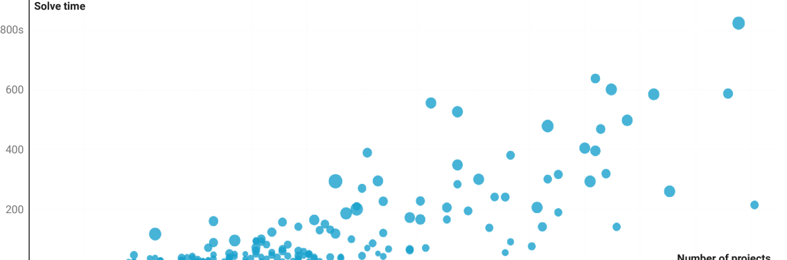
To evaluate the performance of computing Lindahl equilibrium via Eq. 14, we implemented it using the MOSEK solver and applied it to the participatory budgeting datasets in the Pabulib repository (Faliszewski et al., 2023). We find that the program can be solved quite quickly, with solve times shown in Figure 2. The longest solve time we encountered was 822s (or 1489s including the time to write down the encoding) for an instance from Warsaw with 14 897 voters (with 11 426 distinct approval sets) and 134 projects.
For the uncapped setting, Zhao and Freund (2023, Section 4.2) present some experiments on the performance of the proportional response dynamics, and find that it outperforms several alternative solution methods.
5.5 Computing Core Allocations for Separable Piecewise-Linear Concave Utilities
We have set up the capped setting with the caps interpreted as an exogenous constraint. An alternative interpretation is as a capped utility function . This view suggests a variety of generalizations: for example, we might want to allow different agents to specify different caps. We can generalize further to separable piecewise-linear concave utilities (SPLC). These are utility functions that can be written as a sum over goods (separable), with the term corresponding to a good being a (non-decreasing) piecewise-linear concave function of . See Figure 3 for an example.
This class of utility functions is well-studied for private goods, both for Fisher markets and Arrow–Debreu exchange markets. For these markets, just as for linear utilities, equilibrium exists and is rational under mild conditions; however computing an equilibrium becomes PPAD-complete (Vazirani and Yannakakis, 2011; Chen and Teng, 2009; Deligkas et al., 2024). A complementary pivot algorithm for computing an equilibrium has been proposed (Garg et al., 2015). This algorithm is based on linear complementarity (Eaves, 1971, 1976), which interestingly can also be used to show existence of Lindahl equilibria (Munagala et al., 2022b, Appendix A).
We leave the problem of computing Lindahl equilibria for SPLC utilities open, but we show how our result for the capped setting can be used to at least compute a core-stable allocation (up to any desired approximation factor). We do this by reducing an SPLC instance to a capped instance (with each piece of the piecewise-linear utilities becoming its own separate good), and show that a Lindahl equilibrium for this instance is core-stable with respect to the SPLC utilities.
We begin with formal definitions. A function with is piecewise-linear concave if it can be decomposed into a finite number of linear segments, specified by their lengths and slopes with . Explicitly, for each , writing for the left endpoint of the th segment, we have for . Figure 3 shows an example.
A utility function is called separable piecewise-linear concave (SPLC) if there exist piecewise-linear concave functions for all such that for all allocations . Note that by subdividing segments if necessary, we may assume that for each project , all agents agree on the total number of segments in as well as their lengths. At the same time, we can choose this common subdivision in a minimal way, so that from one segment to the next, there is always at least one agent whose slope strictly decreases. Let us write for the slope of the th segment of , and let us write for the length of the th segment for project .
Any instance of the public goods problem with SPLC utility functions can be translated into an instance with linear utility functions and with caps, using the following construction.
Definition 0.
Suppose we are given an SPLC instance specified by the slopes and lengths of the segments. We construct a public goods instance with linear utility functions on the same set of agents and the new set of projects with . The project will describe how much of project will be funded in the area of its th segment. Finally, we take valuations .
Let us say that an SPLC instance is well-behaved if the derived instance is cap-sufficient in the sense of Definition 6. This is guaranteed to be the case, for example, if for every agent , the total length of segments with positive slope across all projects is at least . Similar sufficient conditions are used for private goods equilibria (e.g., Vazirani and Yannakakis, 2011, Section 2).
Theorem 8.
Let be a well-behaved instance of the public goods problem with SPLC utilities. Then any zero-respecting Lindahl equilibrium for the instance as constructed in Definition 7 can be transformed into a core-stable allocation for the SPLC instance .
Proof.
Suppose that is a zero-respecting Lindahl equilibrium allocation for . By Corollary 11, is Pareto-optimal. Note that we always have by concavity, and for at least one agent the inequality is strict (by minimality of the chosen common subdivision). Thus, Pareto-optimality implies that if then (which equals ). This allows us to define an allocation for instance by setting . We now argue that is core stable.
Suppose not, and there is some blocking coalition and objection such that and for all , we have , with strict inequality for at least . We construct a core objection for , contradicting its core stability (Proposition 9). For each , let be chosen minimal such that . Then set for and , as well as for . Then it is easy to see that for all , and similarly for all , and thus is a core deviation to , a contradiction. ∎
6 Conclusion
We have developed a new class of convex programs that can be used to efficiently compute Lindahl equilibria both in the uncapped and the capped setting. These new programs open up many opportunities for future research.
In the uncapped setting, our new program might lead to new proofs of known results for the well-studied maximum Nash welfare rule. This might include the result about participation incentives of Brandl et al. (2022) or the axiomatic characterization of Guerdjikova and Nehring (2014). Perhaps our program could also shed light on the other uses of the Eisenberg–Gale program across statistics, information theory, and medical imaging, as discussed in Section 1.2. For the capped setting, our computability result has implications for the discrete public goods model, because it allows the efficient implementation of the 9.27-approximation to the core obtained by Munagala et al. (2022b), rather than having to rely on their 67.37-approximation. Munagala et al. (2022b) used Lindahl equilibrium as a black box to obtain their approximation result; reasoning about the structure of our convex program program might lead to even better bounds.
Since our focus has been on computational questions, we have not considered strategic aspects. Lindahl equilibrium is well-known to have high informational requirements, and in particular we need to know the truthful valuations of the agents to compute it. Interpreted as a decision rule (Gul and Pesendorfer, 2020), Lindahl equilibrium is not strategyproof and can be manipulated both in a free-riding sense (Brandl et al., 2021, Section 5.3), and in some paradoxical ways (Aziz et al., 2020, Theorem 3(ii)), even in the uncapped setting. Manipulability is unavoidable if one desires a Pareto-efficient and core-stable solution, both in the uncapped setting (Brandl et al., 2021, Theorem 2 and Theorem 3) and in the capped setting (Bei et al., 2024, Theorem 6.2). These impossibilities apply even for approval (0/1) preferences. For more general linear utilities, strategyproofness is only attainable by dictatorial-type rules (Hylland, 1980), even in the uncapped setting.
We leave several interesting technical questions open. Is the optimum of our program unique in utilities? This is known to be true for the uncapped setting, by strict convexity (in utilities) of the Eisenberg–Gale program. Can we develop first-order methods for the capped settings, or derive a natural dynamics converging to an equilibrium? Applying mirror descent to our program does not appear to lead to a nice closed-form update like in the uncapped setting. Finally, can the cap constraint be generalized? For example, one could apply cap constraints on the total spending of sets of public goods. This would allow us to model multi-issue and multi-round decision making settings (see, e.g., Banerjee et al., 2023, Section 5). It would also allow us to embed private goods in the model (as in Conitzer et al., 2017), and potentially connect the notions of Fisher market equilibrium and Lindahl equilibrium.
References
- (1)
- Airiau et al. (2023) Stéphane Airiau, Haris Aziz, Ioannis Caragiannis, Justin Kruger, Jérôme Lang, and Dominik Peters. 2023. Portioning using ordinal preferences: Fairness and efficiency. Artificial Intelligence 314 (2023), 103809. doi:10.1016/j.artint.2022.103809
- Aziz et al. (2020) Haris Aziz, Anna Bogomolnaia, and Hervé Moulin. 2020. Fair mixing: The case of dichotomous preferences. ACM Transactions on Economics and Computation (TEAC) 8, 4, Article 18 (2020), 27 pages. doi:10.1145/3417738
- Aziz et al. (2017) Haris Aziz, Markus Brill, Vincent Conitzer, Edith Elkind, Rupert Freeman, and Toby Walsh. 2017. Justified Representation in approval-based committee voting. Social Choice and Welfare 48, 2 (2017), 461–485. doi:10.1007/s00355-016-1019-3
- Aziz et al. (2023a) Haris Aziz, Xinhang Lu, Mashbat Suzuki, Jeremy Vollen, and Toby Walsh. 2023a. Best-of-both-worlds fairness in committee voting. arXiv:2303.03642 [cs.GT] https://arxiv.org/abs/2303.03642
- Aziz et al. (2023b) Haris Aziz, Evi Micha, and Nisarg Shah. 2023b. Group Fairness in Peer Review. In Advances in Neural Information Processing Systems, Vol. 36. 64885–64895. https://proceedings.neurips.cc/paper_files/paper/2023/file/ccba10dd4e80e7276054222bb95d467c-Paper-Conference.pdf
- Aziz and Shah (2021) Haris Aziz and Nisarg Shah. 2021. Participatory budgeting: Models and approaches. Springer, 215–236. doi:10.1007/978-3-030-54936-7_10
- Banerjee et al. (2023) Siddhartha Banerjee, Vasilis Gkatzelis, Safwan Hossain, Billy Jin, Evi Micha, and Nisarg Shah. 2023. Proportionally fair online allocation of public goods with predictions. In Proceedings of the 32nd International Joint Conference on Artificial Intelligence (IJCAI). 20–28. doi:10.24963/ijcai.2023/3
- Beck (2017) Amir Beck. 2017. First-Order Methods in Optimization. Society for Industrial and Applied Mathematics (SIAM). doi:10.1137/1.9781611974997
- Bei et al. (2024) Xiaohui Bei, Xinhang Lu, and Warut Suksompong. 2024. Truthful cake sharing. Social Choice and Welfare (2024), 1–35. doi:10.1007/s00355-023-01503-0
- Birnbaum et al. (2011) Benjamin Birnbaum, Nikhil R. Devanur, and Lin Xiao. 2011. Distributed algorithms via gradient descent for Fisher markets. In Proceedings of the 12th ACM Conference on Electronic Commerce (EC). 127–136. doi:10.1145/1993574.1993594
- Bogomolnaia et al. (2005) Anna Bogomolnaia, Hervé Moulin, and Richard Stong. 2005. Collective choice under dichotomous preferences. Journal of Economic Theory 122, 2 (2005), 165–184. doi:10.1016/j.jet.2004.05.005
- Brandl et al. (2022) Florian Brandl, Felix Brandt, Matthias Greger, Dominik Peters, Christian Stricker, and Warut Suksompong. 2022. Funding public projects: A case for the Nash product rule. Journal of Mathematical Economics 99 (2022), 102585. doi:10.1016/j.jmateco.2021.102585
- Brandl et al. (2021) Florian Brandl, Felix Brandt, Dominik Peters, and Christian Stricker. 2021. Distribution rules under dichotomous preferences: two out of three ain’t bad. In Proceedings of the 22nd ACM Conference on Economics and Computation (EC). 158–179. doi:10.1145/3465456.3467653
- Brandt et al. (2024) Felix Brandt, Matthias Greger, Erel Segal-Halevi, and Warut Suksompong. 2024. Coordinating charitable donations. arXiv:2305.10286 [econ.TH]
- Caragiannis et al. (2019) Ioannis Caragiannis, David Kurokawa, Hervé Moulin, Ariel D Procaccia, Nisarg Shah, and Junxing Wang. 2019. The unreasonable fairness of maximum Nash welfare. ACM Transactions on Economics and Computation (TEAC) 7, 3 (2019), 1–32. doi:10.1145/3355902
- Caragiannis et al. (2024) Ioannis Caragiannis, Evi Micha, and Nisarg Shah. 2024. Proportional Fairness in Non-Centroid Clustering. In Proceedings of the 38th Annual Conference on Neural Information Processing Systems (NeurIPS). https://openreview.net/forum?id=Actjv6Wect
- Chaudhury et al. (2022) Bhaskar Ray Chaudhury, Linyi Li, Mintong Kang, Bo Li, and Ruta Mehta. 2022. Fairness in Federated Learning via Core-Stability. In Advances in Neural Information Processing Systems, Vol. 35. 5738–5750. PDF at proceedings.neurips.cc.
- Chen et al. (2019) Xingyu Chen, Brandon Fain, Liang Lyu, and Kamesh Munagala. 2019. Proportionally fair clustering. In Proceedings of the 36th International Conference on Machine Learning (ICML). PMLR, 1032–1041. https://proceedings.mlr.press/v97/chen19d.html
- Chen and Teng (2009) Xi Chen and Shang-Hua Teng. 2009. Spending is not easier than trading: on the computational equivalence of Fisher and Arrow-Debreu equilibria. In Proceedings of the 20th International Symposium on Algorithms and Computation (ISAAC). 647–656.
- Cheng et al. (2020) Yu Cheng, Zhihao Jiang, Kamesh Munagala, and Kangning Wang. 2020. Group fairness in committee selection. ACM Transactions on Economics and Computation (TEAC) 8, 4, Article 23 (2020), 18 pages. doi:10.1145/3417750
- Cole et al. (2017) Richard Cole, Nikhil R. Devanur, Vasilis Gkatzelis, Kamal Jain, Tung Mai, Vijay V. Vazirani, and Sadra Yazdanbod. 2017. Convex program duality, Fisher markets, and Nash social welfare. In Proceedings of the 2017 ACM Conference on Economics and Computation (EC). 459–460. doi:10.1145/3033274.3085109
- Conitzer et al. (2017) Vincent Conitzer, Rupert Freeman, and Nisarg Shah. 2017. Fair public decision making. In Proceedings of the 2017 ACM Conference on Economics and Computation (EC). 629–646. doi:10.1145/3033274.3085125
- Cover (1984) Thomas Cover. 1984. An algorithm for maximizing expected log investment return. IEEE Transactions on Information Theory 30, 2 (1984), 369–373. doi:10.1109/TIT.1984.1056869
- Csiszár (1974) Imre Csiszár. 1974. On the computation of rate-distortion functions (corresp.). IEEE Transactions on Information Theory 20, 1 (1974), 122–124. doi:10.1109/TIT.1974.1055146
- Csiszár (1984) Imre Csiszár. 1984. Information geometry and alternating minimization procedures. Statistics and Decisions Supplemental Issue No. 1 (1984), 205–237. https://dominik-peters.de/archive/csiszar1984.pdf
- Deligkas et al. (2024) Argyrios Deligkas, John Fearnley, Alexandros Hollender, and Themistoklis Melissourgos. 2024. Constant inapproximability for Fisher markets. In Proceedings of the 25th ACM Conference on Economics and Computation (EC). 13–39. doi:10.1145/3670865.3673533
- Devanur et al. (2008) Nikhil R. Devanur, Christos H. Papadimitriou, Amin Saberi, and Vijay V. Vazirani. 2008. Market equilibrium via a primal–dual algorithm for a convex program. Journal of the ACM (JACM) 55, 5 (2008), 1–18. doi:10.1145/1411509.1411512
- Eaves (1971) B. Curtis Eaves. 1971. On the basic theorem of complementarity. Mathematical Programming 1, 1 (1971), 68–75. doi:10.1007/BF01584073
- Eaves (1976) B. Curtis Eaves. 1976. A finite algorithm for the linear exchange model. Journal of Mathematical Economics 3, 2 (1976), 197–203. doi:10.1016/0304-4068(76)90028-8
- Ebadian and Micha (2025) Soroush Ebadian and Evi Micha. 2025. Boosting Sortition via Proportional Representation. In Proceedings of 24th International Conference on Autonomous Agents and Multiagent Systems (AAMAS). Forthcoming.
- Eisenberg (1961) Edmund Eisenberg. 1961. Aggregation of utility functions. Management Science 7, 4 (1961), 337–350. doi:10.1287/mnsc.7.4.337
- Eisenberg and Gale (1959) Edmund Eisenberg and David Gale. 1959. Consensus of subjective probabilities: The pari-mutuel method. The Annals of Mathematical Statistics 30, 1 (1959), 165–168. doi:10.1214/aoms/1177706369
- Fain et al. (2016) Brandon Fain, Ashish Goel, and Kamesh Munagala. 2016. The core of the participatory budgeting problem. In Proceedings of the 12th International Conference on Web and Internet Economics (WINE). 384–399. doi:10.1007/978-3-662-54110-4_27
- Fain et al. (2018) Brandon Fain, Kamesh Munagala, and Nisarg Shah. 2018. Fair allocation of indivisible public goods. In Proceedings of the 2018 ACM Conference on Economics and Computation (EC). 575–592. doi:10.1145/3219166.3219174
- Faliszewski et al. (2023) Piotr Faliszewski, Jarosław Flis, Dominik Peters, Grzegorz Pierczyński, Piotr Skowron, Dariusz Stolicki, Stanisław Szufa, and Nimrod Talmon. 2023. Participatory budgeting: Data, tools, and analysis. In Proceedings of the 32nd International Joint Conference on Artificial Intelligence (IJCAI). 2667–2674. doi:10.24963/ijcai.2023/297
- Foley (1970) Duncan K. Foley. 1970. Lindahl’s solution and the core of an economy with public goods. Econometrica (1970), 66–72. doi:10.2307/1909241
- Garg et al. (2015) Jugal Garg, Ruta Mehta, Milind Sohoni, and Vijay V. Vazirani. 2015. A complementary pivot algorithm for market equilibrium under separable, piecewise-linear concave utilities. SIAM J. Comput. 44, 6 (2015), 1820–1847. doi:10.1137/140971002
- Garg et al. (2021) Nikhil Garg, Ashish Goel, and Benjamin Plaut. 2021. Markets for public decision-making. Social Choice and Welfare 56, 4 (2021), 755–801. doi:10.1007/s00355-020-01298-4
- Greaves and Cotton-Barratt (2023) Hilary Greaves and Owen Cotton-Barratt. 2023. A bargaining-theoretic approach to moral uncertainty. Journal of Moral Philosophy 1, aop (2023), 1–43. doi:10.1163/17455243-20233810
- Guerdjikova and Nehring (2014) Ani Guerdjikova and Klaus Nehring. 2014. Weighing experts, weighing sources: The diversity value. (2014). https://dominik-peters.de/archive/guerdjikova2014.pdf Working Paper.
- Gul and Pesendorfer (2020) Faruk Gul and Wolfgang Pesendorfer. 2020. Lindahl equilibrium as a collective choice rule. arXiv:2008.09932 [econ.TH]
- Hylland (1980) Aanund Hylland. 1980. Strategyproofness of voting procedures with lotteries as outcomes and infinite sets of strategies. (1980). https://www.sv.uio.no/econ/personer/vit/aanundh/upubliserte-artikler-og-notater/Strategy%20Proofness%5B1%5D.pdf unpublished.
- Jiang et al. (2020) Zhihao Jiang, Kamesh Munagala, and Kangning Wang. 2020. Approximately stable committee selection. In Proceedings of the 52nd Annual ACM SIGACT Symposium on Theory of Computing (STOC). 463–472. doi:10.1145/3357713.3384238
- Kaneko (1977) Mamoru Kaneko. 1977. The ratio equilibrium and a voting game in a public goods economy. Journal of Economic Theory 16, 2 (1977), 123–136. doi:10.1016/0022-0531(77)90001-1
- Kellerhals and Peters (2024) Leon Kellerhals and Jannik Peters. 2024. Proportional Fairness in Clustering: A Social Choice Perspective. In Proceedings of the 38th Annual Conference on Neural Information Processing Systems (NeurIPS). https://openreview.net/forum?id=KsLX5pFpOs
- Komiya (1988) Hidetoshi Komiya. 1988. Elementary proof for Sion’s minimax theorem. Kodai Mathematical Journal 11, 1 (1988), 5 – 7. doi:10.2996/kmj/1138038812
- Lackner and Skowron (2023) Martin Lackner and Piotr Skowron. 2023. Multi-Winner Voting with Approval Preferences. Springer. doi:10.1007/978-3-031-09016-5
- Li et al. (2018) Yen-Huan Li, Carlos A. Riofrio, and Volkan Cevher. 2018. A general convergence result for mirror descent with Armijo line search. arXiv:1805.12232 [math.OC]
- Lindahl (1919) Erik Lindahl. 1919. Just taxation—a positive solution. Translated from German (Die Gerechtigkeit der Besteuerung, Lund 1919, Part I, Chap. 4, pp. 85–98: Positive Lösung) by Elizabeth Henderson. In Classics in the Theory of Public Finance, Richard A. Musgrave and Alan T. Peacock (Eds.). Palgrave Macmillan (1958), 168–176. doi:10.1007/978-1-349-23426-4_11
- Mas-Colell and Silvestre (1989) Andreu Mas-Colell and Joaquim Silvestre. 1989. Cost share equilibria: A Lindahlian approach. Journal of Economic Theory 47, 2 (1989), 239–256. doi:10.1016/0022-0531(89)90019-7
- Michorzewski et al. (2020) Marcin Michorzewski, Dominik Peters, and Piotr Skowron. 2020. Price of fairness in budget division and probabilistic social choice. In Proceedings of the 34th AAAI Conference on Artificial Intelligence (AAAI). 2184–2191. doi:10.1609/aaai.v34i02.5594
- Moore (2006) James C. Moore. 2006. General Equilibrium and Welfare Economics: An Introduction. Springer. doi:10.1007/978-3-540-32223-8
- Moulin (2004) Hervé Moulin. 2004. Fair Division and Collective Welfare. MIT Press. doi:10.7551/mitpress/2954.001.0001
- Munagala et al. (2022a) Kamesh Munagala, Yiheng Shen, and Kangning Wang. 2022a. Auditing for core stability in participatory budgeting. In Proceedings of the 18th International Conference on Web and Internet Economics (WINE). 292–310. doi:10.1007/978-3-031-22832-2_17
- Munagala et al. (2022b) Kamesh Munagala, Yiheng Shen, Kangning Wang, and Zhiyi Wang. 2022b. Approximate core for committee selection via multilinear extension and market clearing. In Proceedings of the 2022 Annual ACM-SIAM Symposium on Discrete Algorithms (SODA). 2229–2252. doi:10.1137/1.9781611977073.89
- Nash (1950) John F. Nash. 1950. The bargaining problem. Econometrica 18, 2 (1950), 155–162. doi:10.2307/1907266
- O’Donoghue et al. (2016) Brendan O’Donoghue, Eric Chu, Neal Parikh, and Stephen Boyd. 2016. Conic Optimization via Operator Splitting and Homogeneous Self-Dual Embedding. Journal of Optimization Theory and Applications 169, 3 (June 2016), 1042–1068. http://stanford.edu/~boyd/papers/scs.html
- Peters (2019) Dominik Peters. 2019. Economic design for effective altruism. The Future of Economic Design: The Continuing Development of a Field as Envisioned by Its Researchers (2019), 381–388. doi:10.1007/978-3-030-18050-8_53
- Peters (2025) Dominik Peters. 2025. The Core of Approval-Based Committee Elections with Few Candidates. arXiv:2501.18304 [cs.GT]
- Peters et al. (2021b) Dominik Peters, Grzegorz Pierczyński, Nisarg Shah, and Piotr Skowron. 2021b. Market-based explanations of collective decisions. In Proceedings of the 35th AAAI Conference on Artificial Intelligence (AAAI). 5656–5663. doi:10.1609/aaai.v35i6.16710
- Peters et al. (2021a) Dominik Peters, Grzegorz Pierczyński, and Piotr Skowron. 2021a. Proportional Participatory Budgeting with Additive Utilities. In Advances in Neural Information Processing Systems, Vol. 34. 12726–12737. https://proceedings.neurips.cc/paper_files/paper/2021/file/69f8ea31de0c00502b2ae571fbab1f95-Paper.pdf
- Peters and Skowron (2020) Dominik Peters and Piotr Skowron. 2020. Proportionality and the limits of welfarism. In Proceedings of the 21st ACM Conference on Economics and Computation (EC). 793–794. Full version arXiv:1911.11747.
- Pierczyński and Skowron (2022) Grzegorz Pierczyński and Piotr Skowron. 2022. Core-stable committees under restricted domains. In Proceedings of the 18th International Conference on Web and Internet Economics (WINE). 311–329. doi:10.1007/978-3-031-22832-2_18
- Rey and Maly (2023) Simon Rey and Jan Maly. 2023. The (computational) social choice take on indivisible participatory budgeting. arXiv:2303.00621 [cs.GT] https://arxiv.org/abs/2303.00621
- Rockafellar (1970) Ralph Tyrell Rockafellar. 1970. Convex Analysis. Princeton Mathematical Series, Vol. 28. Princeton University Press. doi:10.1515/9781400873173
- Ruszczynski (2011) Andrzej Ruszczynski. 2011. Nonlinear Optimization. Princeton University Press. doi:10.2307/j.ctvcm4hcj
- Samuelson (1954) Paul A. Samuelson. 1954. The pure theory of public expenditure. The Review of Economics and Statistics 36, 4 (1954), 387–389. doi:10.2307/1925895
- Shmyrev (1983) Vadim I Shmyrev. 1983. On an approach to the determination of equilibrium in elementary exchange models. In Doklady Akademii Nauk SSSR, Vol. 268:5. 1062–1066. https://www.mathnet.ru/eng/dan10141 (In Russian).
- Shmyrev (2009) Vadim I. Shmyrev. 2009. An algorithm for finding equilibrium in the linear exchange model with fixed budgets. Journal of Applied and Industrial Mathematics 3, 4 (2009), 505. doi:10.1134/S1990478909040097
- Suzuki and Vollen (2024) Mashbat Suzuki and Jeremy Vollen. 2024. Maximum flow is fair: A network flow approach to committee voting. In Proceedings of the 25th ACM Conference on Economics and Computation (EC). 964–983. doi:10.1145/3670865.3673603
- van den Nouweland (2015) Anne van den Nouweland. 2015. Lindahl and equilibrium. In Individual and Collective Choice and Social Welfare: Essays in Honor of Nick Baigent, Constanze Binder, Giulio Codognato, Miriam Teschl, and Yongsheng Xu (Eds.). Springer, 335–362. doi:10.1007/978-3-662-46439-7_18
- Vardi and Lee (1993) Yehuda Vardi and D. Lee. 1993. From image deblurring to optimal investments: Maximum likelihood solutions for positive linear inverse problems. Journal of the Royal Statistical Society Series B: Statistical Methodology 55, 3 (1993), 569–598. doi:10.1111/j.2517-6161.1993.tb01925.x
- Vardi et al. (1985) Yehuda Vardi, Larry A Shepp, and Linda Kaufman. 1985. A statistical model for positron emission tomography. Journal of the American statistical Association 80, 389 (1985), 8–20. doi:10.1080/01621459.1985.10477119
- Vazirani (2012) Vijay V. Vazirani. 2012. The notion of a rational convex program, and an algorithm for the Arrow-Debreu Nash bargaining game. Journal of the ACM (JACM) 59, 2 (2012), 1–36. doi:10.1145/2160158.2160160
- Vazirani and Yannakakis (2011) Vijay V. Vazirani and Mihalis Yannakakis. 2011. Market equilibrium under separable, piecewise-linear, concave utilities. Journal of the ACM (JACM) 58, 3 (2011), 1–25. doi:10.1145/1970392.1970394
- Vishnoi (2021) Nisheeth K. Vishnoi. 2021. Algorithms for Convex Optimization. Cambridge University Press. doi:10.1017/9781108699211 https://convex-optimization.github.io/.
- Wu and Zhang (2007) Fang Wu and Li Zhang. 2007. Proportional response dynamics leads to market equilibrium. In Proceedings of the 39th Annual ACM Symposium on Theory of Computing (STOC). 354–363. doi:10.1145/1250790.1250844
- Zhang (2011) Li Zhang. 2011. Proportional response dynamics in the Fisher market. Theoretical Computer Science 412, 24 (2011), 2691–2698. doi:10.1016/j.tcs.2010.06.021
- Zhao (2023) Renbo Zhao. 2023. Convergence rate analysis of the multiplicative gradient method for PET-type problems. Operations Research Letters 51, 1 (2023), 26–32. doi:10.1016/j.orl.2022.11.010
- Zhao and Freund (2023) Renbo Zhao and Robert M. Freund. 2023. Analysis of the Frank–Wolfe method for convex composite optimization involving a logarithmically-homogeneous barrier. Mathematical programming 199, 1 (2023), 123–163. doi:10.1007/s10107-022-01820-9