Parallel Domain-Decomposition Algorithms for Complexity Certification of Branch-and-Bound Algorithms for Mixed-Integer Linear and Quadratic Programming

Abstract

When implementing model predictive control (MPC) for hybrid systems with a linear or a quadratic performance measure, a mixed-integer linear program (MILP) or a mixed-integer quadratic program (MIQP) needs to be solved, respectively, at each sampling instant. Recent work has introduced the possibility to certify the computational complexity of branch-and-bound (B&B) algorithms when solving MILP and MIQP problems formulated as multi-parametric MILPs (mp-MILPs) and mp-MIQPs. Such a framework allows for computing the worst-case computational complexity of standard B&B-based MILP and MIQP solvers, quantified by metrics such as the total number of LP/QP iterations and B&B nodes. These results are highly relevant for real-time hybrid MPC applications. In this paper, we extend this framework by developing parallel, domain-decomposition versions of the previously proposed algorithm, allowing it to scale to larger problem sizes and enable the use of high-performance computing (HPC) resources. Furthermore, to reduce peak memory consumption, we introduce two modifications to the existing (serial) complexity certification framework, integrating them into the proposed parallel algorithms. Numerical experiments show that the parallel algorithms significantly reduce computation time while maintaining the correctness of the original framework.

I Introduction

To determine the optimal control inputs in model predictive control (MPC), an optimization problem is solved at each time step. When MPC is applied to hybrid systems that contain both continuous and discrete dynamics, the resulting optimization problems, depending on the chosen performance measure, can be formulated as mixed-integer linear programs (MILPs) (for $1$-norm or $\infty$-norm) or mixed-integer quadratic programs (MIQPs) (for $2$-norm) [1, 2, 3]. In MPC applications, system states and reference signals are usually assumed to belong to a closed (in many applications polyhedral) set and are considered as parameters in the optimization problem. This allows for the formulation of these problems as multi-parametric MILP (mp-MILP) and mp-MIQP problems [4]. Computing the solutions to these optimization problems parametrically offers the advantage of shifting most of the online computational burden offline [5]. However, storing pre-computed solutions might require a significant amount of memory and can become increasingly complex for high-dimensional problems, limiting its use on embedded hardware. The traditional alternative to solving these optimization problems parametrically offline is to solve these problems online in real-time, which in the MPC application considered in this work means solving MILPs and MIQPs under real-time constraints. In such a setup, it is clearly of high interest to be able to obtain relevant bounds on the worst-case computational complexity. Such guarantees on the worst-case computational complexity for LPs, QPs, MILPs, and MIQPs have been provided in, e.g., [6],  [7, 8],  [9, 10], and [11, 12, 13], respectively. In particular, the unified certification method presented in [13] focuses on determining the worst-case computational complexity for solving MILP and MIQP instances to optimality that originate from a given mp-MILP or mp-MIQP and a corresponding polyhedral parameter set, when employing the standard branch-and-bound (B&B) algorithm. This certification is performed through the process of recursively partitioning the parameter space based on the solver state. The complexity measures considered in [12, 9, 13] are the number of linear systems of equations that are solved in the subsolver of B&B (the iteration number) and the number of relaxations (nodes) required to be solved in B&B. Nevertheless, this method might require a considerable amount of processing time and memory, particularly as the size of the problem increases.

The primary contribution of this work is proposing complexity certification algorithms that can be executed in parallel, with the aim to distribute both the computational load and memory requirements across a (potentially large) number of workers [14, 15, 16]. In particular, our objective is to introduce parallel versions of our previously presented complexity certification framework, which will open up for the consideration of larger problem sizes and the certification of more challenging problems. This not only improves computation time but also enables the use of high-performance computing (HPC) to further expand the range of problem sizes that can be certified within a reasonable timeframe.

When certifying larger problem instances in this work, a significant increase in peak memory consumption was observed. To address this, we propose two key modifications to the (serial) complexity certification framework presented in [13]. These modifications are then incorporated into the proposed parallel algorithms to reduce peak memory usage. To summarize, the main contributions of this paper are:

• Two parallel algorithms for certifying the complexity of B&B-based MILP and MIQP solvers.

• Two novel strategies for reducing peak memory consumption.

II Problem formulation

In this work, we consider mp-MILP problems of the form

$$\min_{x}\quad c^{T}x$$ (1a)

$$\mathcal{P}_{\text{mpMILP}}(\theta):\hskip 5.69046pt\textrm{s.t.}\quad Ax\leqslant b(\theta),$$ (1b)

$$x_{i}\in\{0,1\},\hskip 5.69046pt\forall i\in\mathcal{B},$$ (1c)

where $x\in\mathbb{R}^{n_{c}}\times\{0,1\}^{n_{b}}$ is the decision variable vector with $n=n_{c}+n_{b}$ components, including $n_{c}$ continuous and $n_{b}$ binary components, and $\theta$ is the parameter vector belonging to the polyhedral set $\Theta_{0}\subset\mathbb{R}^{n_{\theta}}$. The objective function in (1) is defined by $c\in\mathbb{R}^{n}$, and the feasible set is characterized by the matrix $A\in\mathbb{R}^{m\times n}$ and the vector $b(\theta)$, which is an affine function of $\theta$, given by $b(\theta)=b+W\theta$, where $b\in\mathbb{R}^{m}$ and $W\in\mathbb{R}^{m\times n_{\theta}}$. Moreover, $\mathcal{B}$ represents the index set of the binary decision variables. The problem (1) is non-convex and is known to be $\mathcal{NP}$-hard [17].

A convex relaxation of (1) can be derived by relaxing the binary constraints (1c) as follows

$$\min_{x}\quad c^{T}x$$ (2a)

$$\mathcal{P}_{\text{mpLP}}(\theta):\hskip 5.69046pt\textrm{s.t.}\quad Ax\leqslant b(\theta),$$ (2b)

$$0\leqslant x_{i}\leqslant 1,\hskip 5.69046pt\forall i\in\mathcal{B},$$ (2c)

$$x_{i}=0,\hskip 2.27626pt\forall i\in\mathcal{B}_{0},\hskip 2.84544ptx_{i}=1,\hskip 2.27626pt\forall i\in\mathcal{B}_{1},$$ (2d)

which is in the form of an mp-LP problem. Here, $\mathcal{B}_{0}\subseteq\mathcal{B}$ and $\mathcal{B}_{1}\subseteq\mathcal{B}$ represent the indices of binary variables fixed to $0$ and $1$, respectively, with $\mathcal{B}_{0}\cap\mathcal{B}_{1}=\emptyset$.

For a fixed parameter vector $\bar{\theta}\in\Theta_{0}$, the problem (1) is simplified to the (non-parametric) MILP problem $\mathcal{P}_{\text{MILP}}(\bar{\theta})$ with $b(\bar{\theta})=b+W\bar{\theta}$. An LP relaxation $\mathcal{P}_{\text{LP}}(\bar{\theta})$ of the MILP problem $\mathcal{P}_{\text{MILP}}(\bar{\theta})$ can be obtained from (2) by fixing $\theta$ to $\bar{\theta}$.

We additionally consider mp-MIQP problems of the form

$$\vskip 2.84544pt\min_{x}\quad \frac{1}{2}x^{T}Hx+f(\theta)^{T}x$$ (3a)

$$\mathcal{P}_{\text{mpMIQP}}(\theta):\hskip 8.5359pt\textrm{s.t.}\quad Ax\leqslant b(\theta),$$ (3b)

$$x_{i}\in\{0,1\},\hskip 8.5359pt\forall i\in\mathcal{B},$$ (3c)

where $H\in\mathbb{S}_{++}^{n}$ and $f(\theta)$ is an affine function of $\theta$, given by $f(\theta)=f+f_{\theta}\theta$, with $f\in\mathbb{R}^{n}$ and $f_{\theta}\in\mathbb{R}^{n\times n_{\theta}}$. The decision variables, parameter vector, and feasible set are defined similarly to those in (1).

A convex relaxation $\mathcal{P}_{\text{mpQP}}(\theta)$ of (3) can similarly be derived by relaxing the binary constraints (3c) into constraints (2c). Furthermore, for a fixed parameter $\bar{\theta}\in\Theta_{0}$, the (non-parametric) MIQP problem $\mathcal{P}_{\text{MIQP}}(\bar{\theta})$ is obtained from (3) with $b(\bar{\theta})=b+W\bar{\theta}$ and $f(\bar{\theta})=f+f_{\theta}\bar{\theta}$.

A commonly used technique to compute the solutions of MILPs and MIQPs is branch and bound (B&B) [17]. This method explores a binary search tree in search for a possible optimal solution, where each node within the tree represents a convex (LP/QP) relaxation. The relaxations can be solved using an LP/QP solver, such as the simplex or active-set method [18]. An important feature of B&B is that the results from the solutions to the relaxations can be used to prove that parts of the tree can be pruned from explicit exploration. Such pruning can be done if one of the following conditions is satisfied in a node [17]:

1. The objective function value of the relaxation (the lower bound), denoted as $\stackunder[1.2pt]{$J$}{\rule{3.44444pt}{0.32289pt}}$, is greater than the objective function value of the best-known integer-feasible solution so far (the upper bound), denoted as $\bar{J}$. In other words, $\stackunder[1.2pt]{$J$}{\rule{3.44444pt}{0.32289pt}}\geq\bar{J}$, which is referred to as the dominance cut. The infeasibility cut is a special case of this, where $\stackunder[1.2pt]{$J$}{\rule{3.44444pt}{0.32289pt}}=\infty$.

2. The solution to the relaxation, denoted $\stackunder[1.2pt]{$x$}{\rule{3.44444pt}{0.32289pt}}$, is integer feasible, which is referred to as the integer-feasibility cut.

If none of these conditions holds in a node, the tree is branched at that node by fixing a relaxed binary variable, which generates two new nodes (child nodes to the parent node). In this paper, we denote a B&B node representing a relaxation by $\eta\triangleq\left(\mathcal{B}_{0},\mathcal{B}_{1}\right)$, where $\mathcal{B}_{0}$ and $\mathcal{B}_{1}$ are defined in (2d). The first node, i.e., the root node, is thus denoted $\eta_{0}=\left(\emptyset,\emptyset\right)$, where all the binary variables have been relaxed. Refer to [17] for a detailed description of the B&B method.

Throughout this paper, $\mathbb{N}_{0}$ denotes the set of nonnegative integers, $\mathbb{N}_{1:N}$ represents the finite set $\{1,\dots,N\}$, and $\{\mathcal{C}^{i}\}_{i=1}^{N}$ denotes a finite collection $\{\mathcal{C}^{1},\dots,\mathcal{C}^{N}\}$ of $N$ elements. When $N$ is unimportant, we use $\{\mathcal{C}^{i}\}_{i}$ instead.

III Serial complexity certification framework

This section briefly reviews the (serial) complexity certification framework for standard B&B algorithms for MILPs and MIQPs presented in [13], referred to as the B&BCert algorithm. The framework takes an mp-MILP (1) or mp-MIQP (3) along with the parameter set $\Theta_{0}$ as inputs and partitions $\Theta_{0}$ based on the computational effort required to reach optimality. Specifically, B&BCert iteratively decomposes $\Theta_{0}$ into regions where the parameters produce the same solver state sequence. The complexity measure, denoted by $\kappa$, quantifies the number of linear systems of equations solved in relaxations (iterations) or the number of B&B nodes explored. Moreover, as shown in [13], the framework can be extended to include other complexity measures, such as the number of floating-point operations (flops).

For clarity and completeness, a version of the B&BCert certification algorithm is provided in Algorithm 1. This algorithm maintains two lists: $\mathcal{S}$, which stores regions that have not yet terminated, and $\mathcal{F}$, which stores the terminated regions. Each tuple $\left(\Theta,\mathcal{T},\kappa_{\text{tot}},\bar{J}\right)$ in $\mathcal{S}$, denoted reg for short, consists of the following elements:

• $\Theta$: the corresponding parameter set.

• $\mathcal{T}=\{\eta_{i}\}_{i}$: a sorted list of pending nodes, corresponding to the local B&B tree within the region.

• $\kappa_{\text{tot}}$: the accumulated complexity measure obtained for the region to reach its current state.

• $\bar{J}(\theta)$: the best-known integer feasible solution (i.e., the upper bound) for all $\theta\in\Theta$.

The initial tuple ($\texttt{reg}^{0}$) passed to Algorithm 1 is $(\Theta^{0},\mathcal{T}^{0},\kappa_{{tot}}^{0},\bar{J}^{0})=(\Theta_{0},\{(\emptyset,\emptyset)\},0,\infty)$, which contains the entire parameter set $\Theta_{0}$ and the root node. The output of the algorithm is a partition of $\Theta_{0}$ along with the corresponding complexity measure.

Algorithm 1 B&BCert: (serial) B&B complexity certification algorithm [13]

1:[l]$\texttt{reg}^{0}=(\Theta^{0},\mathcal{T}^{0},\kappa_{{tot}}^{0},\bar{J}^{0})$

2:Final partition $\mathcal{F}$

3:$\mathcal{F}\leftarrow\emptyset$

4:Push $\texttt{reg}^{0}$ to $\mathcal{S}$

5:while $\mathcal{S}\neq\emptyset$ do

6: Pop reg = $(\Theta,\mathcal{T},\kappa_{{tot}},\bar{J})$ from $\mathcal{S}$

7: if $\mathcal{T}=\emptyset$ then

8: Add reg to $\mathcal{F}$

9: else

10: Pop new node $\eta$ from $\mathcal{T}$

11: $\{(\Theta^{j},\kappa^{j},\stackunder[1.2pt]{$J$}{\rule{3.44444pt}{0.32289pt}}^{j})\}_{j=1}^{N}\leftarrow\textsc{solveCert}(\eta,\Theta)$

12: for $j\in\mathbb{N}_{1:N}$ do

13:  $\texttt{reg}^{j}\leftarrow(\Theta^{j},\mathcal{T},\kappa^{j}+\kappa_{tot},\bar{J})$

14:  $\mathcal{S}\leftarrow\textsc{cutCert}$ $(\texttt{reg}^{j},\stackunder[1.2pt]{$J$}{\rule{3.44444pt}{0.32289pt}}^{j},\eta,\mathcal{S})$    

15:Return $\mathcal{F}$

Algorithm 1 follows these main steps for a selected reg at Step 6:

• If no pending nodes remain in $\mathcal{T}$, reg is added to the final partition $\mathcal{F}$ (Step 8).

• Otherwise, a node is selected from $\mathcal{T}$ (Step 10), and its corresponding (LP/QP) relaxation is certified using the solveCert subroutine (Step 11). This subroutine partitions the parameter set $\Theta$, associating each resulting subregion $\Theta^{j}$ with the objective function value $\stackunder[1.2pt]{$J$}{\rule{3.44444pt}{0.32289pt}}^{j}(\theta)$ (lower bound) and the required complexity $\kappa^{j}$. An example of solveCert is provided in [8].

• The region is then decomposed into $N$ subregions (Step 13). For each subregion $\Theta^{j}$, the parameter-dependent B&B cut conditions (see Section II, Items 1-3) are evaluated using the cutCert procedure. More details on this procedure can be found in [13, Algorithm 8].

Throughout this paper, we assume that the solveCert function satisfies the properties outlined in Assumption 1 of [13] (which hold for certain subsolvers based on results for mp-LPs and mp-QPs), summarized below. The polyhedral condition in parentheses holds if the inputted $\Theta$ is polyhedral.

Assumption 1

The solveCert function partitions a (polyhedral) parameter set $\Theta$ into a finite collection of (polyhedral) subregions $\{\Theta^{j}\}_{j}$. The value function $\stackunder[1.2pt]{$J$}{\rule{3.44444pt}{0.32289pt}}(\theta)$ is (polyhedral) piecewise affine (PWA) for MILPs and (polyhedral) piecewise quadratic (PWQ) for MIQPs. Additionally, the complexity measure $\kappa(\theta)$ is (polyhedral) piecewise constant (PWC). Moreover, the complexity measure obtained from solveCert is assumed to coincide with that of the corresponding online solver for any $\theta\in\Theta_{0}$.

IV Parallel complexity certification framework

In B&BCert, the entire set $\Theta_{0}$ is processed sequentially, iteratively decomposing it into subregions $\Theta\subseteq\Theta_{0}$ while exploring all pending nodes in the B&B search tree until an optimal solution is found or infeasibility is detected $\forall\theta\in\Theta$. In this section, we extend this approach to enable parallel execution of the certification algorithm for mp-MILPs and mp-MIQPs in (1) and (3), respectively. The following subsections introduce two parallel versions of B&BCert based on domain decomposition, which distributes tasks across available computational resources, referred to as workers. The main processor responsible for this distribution is referred to as the master [16].

IV-A Static domain decomposition

An approach to parallelizing the certification framework is to divide the parameter set $\Theta_{0}$ into smaller subsets, for example, by partitioning it into equally sized boxes. These subregions are then distributed among available processors (workers), with each worker independently applying the B&BCert algorithm to its assigned subset.

The B&BCertStat procedure, detailed in Algorithm 2, implements this static domain decomposition strategy. The worker pool, denoted by $\mathcal{W}$, represents the collection of processors executing tasks concurrently. Starting with the initial tuple $\texttt{reg}^{0}=(\Theta^{0},\mathcal{T}^{0},\kappa_{{tot}}^{0},\bar{J}^{0})=(\Theta_{0},\{(\emptyset,\emptyset)\},0,\infty)$ (as in Algorithm 1), the algorithm partitions $\Theta_{0}$ (Step 5) and distributes the subregions across workers. Each worker $w\in\mathcal{W}$ independently executes B&BCert on its assigned subregion (Step 8). Finally, the results are aggregated into a final partition $\mathcal{F}_{s}$ (Step 9), which includes the partitioned parameter set and corresponding complexity measures.

Algorithm 2 B&BCertStat: Static parallel domain-decomposition complexity certification algorithm

1:[l]$\texttt{reg}^{0}=(\Theta^{0},\mathcal{T}^{0},\kappa_{{tot}}^{0},\bar{J}^{0})$

2:Final partition $\mathcal{F}_{s}$

3:$\mathcal{F}_{s}\leftarrow\emptyset$

4:Initialize worker pool $\mathcal{W}$

5:Partition $\Theta^{0}$ into $n_{p}$ parts $\{\Theta^{k}\}_{k=1}^{n_{p}}$

6:for all $k\in\mathbb{N}_{1:n_{p}}$ in parallel do

7: $\texttt{reg}^{k}\leftarrow\left(\Theta^{k},\mathcal{T}^{0},\kappa_{\text{tot}}^{0},\bar{J}^{0}\right)$

8: $\mathcal{F}^{k}\leftarrow$ B&BCert$(\texttt{reg}^{k})$

9:Append $\mathcal{F}^{k}$ for all $k$ to $\mathcal{F}_{s}$

10:Return $\mathcal{F}_{s}$

Algorithm 2 follows the master-worker paradigm [16], where the master partitions the initial parameter set, assigns subregions to workers, and collects the results. While conceptually straightforward, this approach does not exploit the problem’s inherent structure. It potentially introduces initial artificial regions, leading to redundant computations and a potential reduction in overall efficiency.

IV-B Dynamic domain decomposition

This section introduces a parallel method that dynamically distributes computational tasks among available resources while leveraging the problem’s solution structure. Unlike static decomposition, this approach assigns tasks to workers based on the relaxation’s solution structure, aiming to improve resource utilization efficiency and minimize redundant computations.

The B&BCertDyn procedure, detailed in Algorithm 3, implements this dynamic domain decomposition strategy. Similar to Algorithm 1, it maintains two lists: $\mathcal{S}_{d}$ for candidate regions and $\mathcal{F}_{d}$ for terminated regions. The algorithm takes as input an initial tuple $\texttt{reg}^{0}=(\Theta^{0},\mathcal{T}^{0},\kappa_{\text{tot}}^{0},\bar{J}^{0})$ and a user-defined parameter $r\in[0,1]$ that determines the distribution ratio. The output is a partition of $\Theta^{0}$ along with the corresponding complexity measures. Upon its initial invocation, the algorithm starts with $\texttt{reg}^{0}=(\Theta^{0},\mathcal{T}^{0},\kappa_{\text{tot}}^{0},\bar{J}^{0})=(\Theta_{0},\{(\emptyset,\emptyset)\},0,\infty)$ (as in Algorithm 1). Additionally, the algorithm employs the same underlying solveCert and cutCert functions as those in Algorithm 1.

Algorithm 3 B&BCertDyn: Dynamic parallel domain-decomposition complexity certification algorithm

1:$\texttt{reg}^{0}=(\Theta^{0},\mathcal{T}^{0},\kappa_{\text{tot}}^{0},\bar{J}^{0})$, ratio $r$

2:Final partition $\mathcal{F}_{d}$

3:$\mathcal{F}_{d}\leftarrow\emptyset$

4:Push $\texttt{reg}^{0}$ to $\mathcal{S}_{d}$

5:Initialize worker pool $\mathcal{W}$

6:while $\mathcal{S}_{d}\neq\emptyset$ do

7: Pop $\texttt{reg}=(\Theta,\mathcal{T},\kappa_{\text{tot}},\bar{J})$ from $\mathcal{S}_{d}$

8: if $\mathcal{T}=\emptyset$ then

9: Add reg to $\mathcal{F}_{d}$

10: else

11: Pop new node $\eta$ from $\mathcal{T}$

12: $\{(\Theta^{j},\stackunder[1.2pt]{$J$}{\rule{3.44444pt}{0.32289pt}}^{j},\kappa^{j})\}_{j=1}^{N}\leftarrow\textsc{solveCert}(\eta,\Theta)$

13: for $j\in\mathbb{N}_{1:N}$ do

14:  $\texttt{reg}^{j}\leftarrow(\Theta^{j},\mathcal{T},\kappa^{j}+\kappa_{\text{tot}},\stackunder[1.2pt]{$J$}{\rule{3.44444pt}{0.32289pt}}^{j})$

15:  $\mathcal{S}_{d}\leftarrow\textsc{cutCert}(\texttt{reg}^{j},\stackunder[1.2pt]{$J$}{\rule{3.44444pt}{0.32289pt}}^{j},\eta,\mathcal{S}_{d})$  

16: $\mathcal{S}_{w}\leftarrow$ Pop $\lceil r\ |\mathcal{S}_{d}|\rceil$ tuples from $\mathcal{S}_{d}$

17: for all $k\in\mathbb{N}_{1:|\mathcal{S}_{w}|}$ in parallel do

18:  Pop $\texttt{reg}^{k}$ from $\mathcal{S}_{w}$

19:  [l] $\mathcal{F}^{k}\leftarrow$ B&BCertDyn$(\texttt{reg}^{k},r)$   

20: Append $\mathcal{F}^{k}$ for all $k$ to $\mathcal{F}_{d}$

21:Return $\mathcal{F}_{d}$

Algorithm 3 leverages the fact that each tuple in $\mathcal{S}_{d}$ is processed independently, allowing the distribution of regions across multiple independent workers, as implemented in Steps 18–19. The distribution ratio $r\in[0,1]$ at Step 16 specifies the proportion of regions in $\mathcal{S}_{d}$ to be assigned to workers, where $|\mathcal{S}_{d}|$ denotes the number of tuples in $\mathcal{S}_{d}$. The value of $r$ can be dynamically adjusted based on factors such as the level of the node in the B&B tree, such that at the early stages of the tree, more tasks (regions) are distributed to other workers, while at later stages, fewer regions are distributed. The for loop at Step 17 distributes the fraction $r$ of these regions to available workers in $\mathcal{W}$, while the remaining regions are retained for evaluation by the master.

Each worker then executes the B&BCertDyn function on its assigned tuple $\texttt{reg}^{k}$, recursively invoking Algorithm 3 until termination. Once a worker completes its tasks, it returns the results to the master, which aggregates them into the final partition $\mathcal{F}_{d}$ at Step 20. The algorithm terminates when all workers complete their tasks and no unprocessed regions remain in $\mathcal{S}_{d}$.

Algorithm 3 follows a multiple-master-worker paradigm [16], where each worker can dynamically assume the role of a master, distributing tasks to idle workers (see Fig. 1). By dynamically distributing tasks and concurrently processing regions, Algorithm 3 improves scalability and is well-suited for large-scale certification problems.

Figure 1: Topology of the proposed parallel Algorithm 3.

Remark 1

At Step 19 of Algorithm 3, if the distribution ratio $r$ (input argument) for the worker is set to $0$, then B&BCertDyn executed by the worker reduces to B&BCert, as no further task distribution occurs. Consequently, each worker independently executes Algorithm 1 on its assigned subregion. Upon completing its task and certifying the entire subregion, the worker returns the results directly to the master. In this case, Algorithm 3 follows a master-worker paradigm, where a single master certifies the root node before assigning tasks to workers. This special case closely resembles Algorithm 2, with the key difference that the parameter set is partitioned only after certifying the root node. This ensures that the final partition coincides with the one generated by the serial algorithm, avoiding artificial subdivisions of the parameter set.

IV-C Properties of the parallel algorithms

This section investigates the properties of the proposed parallel algorithms. These algorithms spatially parallelize the serial certification framework across the parameter set, while the exploration of nodes in the B&B search tree remains sequential. The following theorems formally establish that the sequences of B&B nodes explored in Algorithms 2 and 3 are equivalent to those explored by Algorithm 1 (the serial counterpart) for all parameters of interest.

Theorem 1

Let $\mathbb{B}_{s}(\theta)$ denote the sequence of nodes explored by Algorithm 2 (B&BCertStat) applied to the problem (1)/(3) for a fixed $\theta\in\Theta_{0}$ in a terminated region in $\mathcal{F}_{s}$. Moreover, let $\mathbb{B}(\theta)$ represent the sequence of nodes explored by Algorithm 1 (B&BCert) applied to the same problem for that $\theta$ in a terminated region in $\mathcal{F}$. Then, $\mathbb{B}_{s}(\theta)=\mathbb{B}(\theta)$, $\forall\theta\in\Theta_{0}$.

Proof:

Both algorithms start with the same initial tuple $\texttt{reg}^{0}=(\Theta^{0},\mathcal{T}^{0},\kappa_{\text{tot}}^{0},\bar{J}^{0})=(\Theta_{0},\{(\emptyset,\emptyset)\},0,\infty)$, ensuring identical starting conditions. In Algorithm 2, $\Theta_{0}$ is partitioned into artificial regions $\{\Theta^{k}\}_{k=1}^{n_{p}}$, and each such region retains the same initial $\mathcal{T}^{0}$, $\kappa_{\text{tot}}^{0}$, and $\bar{J}^{0}$. By construction, $\cup\Theta^{k}=\Theta_{0}$, ensuring that for any $\theta\in\Theta_{0}$, there is a unique artificial region $\Theta^{k}$ that contains $\theta$.

Now, consider an artificial region $\Theta^{k}$ and a fixed $\theta\in\Theta^{k}$. Algorithm 2 processes $\theta$ by applying B&BCert to the artificial region $\Theta^{k}$, while in Algorithm 1, $\theta$ is processed by applying the exact same steps to the entire parameter set $\Theta_{0}\ni\theta$. Given that the initial node list and upper bound are the same in both algorithms, the node exploration process, including calls to solveCert and cutCert, is performed identically for $\theta$ in both cases. Consequently, the node exploration sequences remain identical in both algorithms for $\theta$, i.e., $\mathbb{B}_{s}(\theta)=\mathbb{B}(\theta)$. Since $\theta$ and $k$ are arbitrarily, this holds $\forall\theta\in\Theta_{k}$, and all $k$, completing the proof. ∎

Therefore, although Algorithm 2 introduces an artificial partitioning of $\Theta_{0}$, potentially resulting in a finer partitioning in $\mathcal{F}_{s}$ compared to $\mathcal{F}$, Theorem 1 ensures that this does not affect the sequence of nodes explored for any $\theta\in\Theta_{0}$. In other words, the correctness of the node exploration process and its equivalence to the serial algorithm are preserved.

Theorem 2

Let $\mathbb{B}^{i}_{d}(\theta)$ denote the sequence of nodes explored by Algorithm 3 (B&BCertDyn) applied to the problem (1)/(3) for a terminated region $\Theta^{i}$ in $\mathcal{F}_{d}$. Moreover, let $\mathbb{B}^{i}(\theta)$ represent the sequence of nodes explored by Algorithm 1 (B&BCert) applied to the same problem for the region $\Theta^{i}$ in $\mathcal{F}$. Then, $\mathbb{B}_{d}^{i}(\theta)=\mathbb{B}^{i}(\theta)$, $\forall\theta\in\Theta^{i}$, and all $i$.

Proof:

Consider Algorithms 1 and 3, both initialized with the same initial tuple $\texttt{reg}^{0}$. Now, consider an iteration of Algorithm 3 starting from Step 7, where a tuple $\texttt{reg}=(\Theta,\mathcal{T},\kappa_{\text{tot}},\bar{J})$ is selected. By inspection, the sequence of operations at Steps 8–15 is identical to Steps 7–14 in Algorithm 1 when processing reg. Algorithm 3 then follows one of the following cases based on the value of $r$:

• $r=0$: In this case, no subregions are distributed among workers, and Algorithm 3 reduces to Algorithm 1. Thus, the sequence of nodes explored in $\Theta^{i}$ remains the same in both algorithms, i.e., $\mathbb{B}^{i}_{d}(\theta)=\mathbb{B}^{i}(\theta)$, $\forall\theta\in\Theta^{i}$.

• $r\neq 0$: In this case, Algorithm 3 dynamically distributes subregions among workers. Let $\texttt{reg}^{k}=(\Theta^{k},\mathcal{T}^{k},\kappa_{\text{tot}}^{k},\bar{J}^{k})$ be selected from $\mathcal{S}_{d}$ at Step 16 and assigned to a worker $w\in\mathcal{W}$. The worker then applies the same steps (from Step 8 to Step 15) to $\texttt{reg}^{k}$, just as Algorithm 1 would process $\texttt{reg}^{k}$ at later iterations.

  If the worker $w$ further distributes subregions to other idling workers by recursively calling B&BCertDyn, the same reasoning applies to each recursion. Each worker processes its assigned subregions independently but follows the same node exploration strategy as the serial algorithm. Hence, the sequence of explored nodes remains consistent as the serial algorithm. Therefore, for any terminated $\Theta^{i}$, Algorithm 3 explores the same sequence of nodes as Algorithm 1, ensuring $\mathbb{B}^{i}_{d}(\theta)=\mathbb{B}^{i}(\theta)$, $\forall\theta\in\Theta^{i},\forall i$.

This completes the proof. ∎

An important observation is that while different parts of the parameter space are generally processed in a different order in the parallel algorithms compared to the serial one, the exploration (and hence certification) of the B&B process for any fixed parameter $\theta\in\Theta_{0}$ remains unique and follows the same order as in the serial algorithm. As a key result, both proposed parallel algorithms yield the same complexity measures for $\theta$ as the serial algorithm. Consequently, these parallel algorithms provide complexity measures that coincide pointwise with the online B&B method for any fixed $\theta\in\Theta_{0}$, as shown in Corollaries 1 and 2.

Corollary 1

Let $\mathbb{B}_{s}(\theta)$ ($\mathbb{B}_{d}(\theta)$) denote the sequence of nodes explored by Algorithm 2 (Algorithm 3) applied to the problem (1)/(3) for any fixed $\theta\in\Theta_{0}$ in a terminated region in $\mathcal{F}_{s}$ ($\mathcal{F}_{d}$). Moreover, let $\mathbb{B}^{*}(\theta)$ represent the sequence of nodes explored to solve the corresponding MILP/MIQP problem for a fixed $\theta$ using the online B&B algorithm (e.g., [13, Algorithm 1]). Then, $\mathbb{B}^{*}(\theta)=\mathbb{B}_{s}(\theta)$ ($=\mathbb{B}_{d}(\theta)$), $\forall\theta\in\Theta_{0}$.

Proof:

The proof directly follows from Theorem 1 in [13], which establishes the pointwise equivalence of the explored nodes in the serial B&BCert and the online B&B algorithms, combined with Theorem 1 (Theorem 2) in this paper. ∎

Corollary 2

Let $\kappa^{*}_{tot}(\theta)$ denote the accumulated complexity measure returned by the online B&B algorithm (e.g., [13, Algorithm 1]) to solve the MILP or MIQP problem for any fixed $\theta\in\Theta_{0}$. The accumulated complexity measure $\kappa_{tot}(\theta):\Theta_{0}\rightarrow\mathbb{N}_{0}$ returned by Algorithm 2 (Algorithm 3) to certify the problem (1) or (3) for a terminated region $\Theta^{i}$ in $\mathcal{F}_{s}$ ($\mathcal{F}_{d}$) satisfies: (i) $\kappa_{tot}(\theta)$ is PWC, and (ii) $\kappa_{tot}=\kappa^{*}_{tot}$, $\forall\theta\in\Theta^{i}$, and all $i$.

Proof:

The proof directly follows from (i) Corollary 2 and (ii) Theorem 2 in [13], which establishes the pointwise equivalence of the complexity measure in the serial B&BCert and the online B&B algorithms, along with Theorem 1 (Theorem 2) in this paper. Moreover, for MILPs where the parameter set is polyhedral and all partitions remain polyhedral, $\kappa_{tot}(\theta)$ is polyhedral PWC. ∎

V Reducing peak resource consumption

Algorithm 1, and consequently the parallel Algorithms 2 and 3, can exhibit high memory demands, particularly as the problem dimension increases. A major contributor to this memory intensity is the storage requirement for the number of tuples maintained in the list $\mathcal{S}$ during execution. In this section, we propose two modifications to Algorithm 1 to reduce the number of stored tuples in $\mathcal{S}$ throughout the algorithm’s execution, thereby lowering peak memory consumption. These refinements are then incorporated into the proposed parallel algorithms.

To implement these improvements, we introduce a variable called state ($\in\{\texttt{none},\texttt{"Fin"},\texttt{"UnFin"},\texttt{"CC"}\}$) for each region, indicating its current state. The meaning of these states is clarified in the following subsections.

V-A Early termination of relaxation’s certification

When evaluating a node within a region in Algorithm 1, the relaxation—either an mp-LP (2) or an mp-QP—is certified using solveCert within $\Theta$ at Step 11. This process can be computationally intensive, particularly at the root node, where the entire parameter set is considered. Additionally, executing the solveCert procedure to completion often generates a large number of regions, which are stored in $\mathcal{S}$, leading to excessive resource consumption.

To address these challenges, we propose temporarily pausing the solveCert procedure after a predetermined number of regions have been generated and processed. This allows certification to be paused if it becomes resource-intensive and resumed later. To implement this approach, each region produced by the solveCert procedure is assigned a state as follows:

• "Fin" (finished): if the mp-LP/mp-QP relaxation in this region has been solved to optimality or determined to be infeasible or unbounded.

• "UnFin" (unfinished): if the solveCert procedure was paused before reaching a conclusive result.

Algorithm 1 is then modified to evaluate cut conditions exclusively in regions with the "Fin" state, while unfinished regions are stored in $\mathcal{S}$ for certification at a later stage. For each unfinished region, the information obtained before pausing is preserved, allowing the solveCert procedure to resume efficiently from the paused state rather than restarting from scratch. This warm-starting capability helps mitigate the computational burden associated with certifying complex subproblems.

V-B Delayed cut-condition evaluation

In Algorithm 1, parameter-dependent cut conditions are evaluated iteratively over a loop for all resulting (finished) regions at Steps 12–14. This evaluation may further partition each $\Theta^{j}$ (e.g., when evaluating dominance cuts or selecting branching indices [13]), which increases the number of tuples stored in $\mathcal{S}$ and, consequently, the memory usage.

To reduce memory consumption, Algorithm 1 can be modified to delay cut condition evaluations. Specifically, instead of evaluating cut conditions at Step 14 for the node corresponding to finished regions, these regions are stored in $\mathcal{S}$ with their state set to "CC" (cut conditions pending). When a region with the "CC" state is later popped from $\mathcal{S}$, cut conditions are evaluated for its corresponding node, and its state is updated to "Fin" (finished). This modification reduces memory usage by deferring region partitioning from evaluating cut conditions, ensuring that $\mathcal{S}$ contains fewer tuples at any given time.

V-C Modified parallel certification algorithm

To minimize peak memory usage, we integrate the techniques outlined in Sections V-A and V-B into the proposed parallel algorithms. In this revised approach, each tuple in $\mathcal{S}$ is expanded to include the lower bound $\stackunder[1.2pt]{$J$}{\rule{3.44444pt}{0.32289pt}}(\theta)$, the region’s state, and the current node $\eta^{c}$, which are used during cut condition evaluation. Consequently, each tuple is now defined as $\texttt{reg}=(\Theta,\mathcal{T},\kappa_{\text{tot}},\bar{J},\stackunder[1.2pt]{$J$}{\rule{3.44444pt}{0.32289pt}},\text{state},\eta^{c})$. At the start of the algorithm, the initial tuple is set to $\texttt{reg}^{0}=(\Theta_{0},\{(\emptyset,\emptyset)\},0,\infty,\infty,\texttt{none},\texttt{none})$.

To update Algorithm 2, these techniques are first incorporated into Algorithm 1 as described, resulting in a modified serial algorithm referred to as the B&BCertMod function. Consequently, Algorithm 2 is updated to include these strategies by replacing the B&BCert function at Step 8 with the modified serial algorithm B&BCertMod.

The updated version of Algorithm 3, incorporating both modifications, is presented in Algorithm 4. In this algorithm, the modifications from Section V-A are implemented at Steps 14 and Steps 16–19, while the modifications described in Section V-B are implemented at Steps 8–9.

Algorithm 4 B&BCertDynMod: Modified dynamic parallel domain-decomposition complexity certification algorithm

1:[l]$\texttt{reg}^{0}=(\Theta^{0},\mathcal{T}^{0},\kappa_{{tot}}^{0},\bar{J}^{0},\stackunder[1.2pt]{$J$}{\rule{3.44444pt}{0.32289pt}}^{0},\text{state}^{0},\eta^{0})$, ratio $r$

2:Final partition $\mathcal{F}_{d}$

3:$\mathcal{F}_{d}\leftarrow\emptyset$

4:Push $\texttt{reg}^{0}$ to $\mathcal{S}_{d}$

5:Initialize worker pool $\mathcal{W}$

6:while $\mathcal{S}_{d}\neq\emptyset$ do

7: Pop $\texttt{reg}=(\Theta,\mathcal{T},\kappa_{\text{tot}},\bar{J},\stackunder[1.2pt]{$J$}{\rule{3.44444pt}{0.32289pt}},\text{state},\eta^{c})$ from $\mathcal{S}_{d}$

8: if $\text{state}=\texttt{"CC"}$ then

9: $\mathcal{S}_{d}\leftarrow\textsc{cutCert}$$(\texttt{reg},\stackunder[1.2pt]{$J$}{\rule{3.44444pt}{0.32289pt}},\eta^{c},\mathcal{S}_{d})$

10: else if $\text{state}=\texttt{"Fin"}$ and $\mathcal{T}=\emptyset$ then

11: Add reg to $\mathcal{F}_{d}$

12: else

13: Pop new node $\eta$ from $\mathcal{T}$

14: [l]$\{(\Theta^{j},\stackunder[1.2pt]{$J$}{\rule{3.44444pt}{0.32289pt}}^{j},\kappa^{j},\text{state}^{j})\}_{j=1}^{N}\leftarrow\textsc{solveCert}(\eta,\Theta,\text{state})$

15: for $j\in\{1,\dots,N\}$ do

16:  if $\text{state}^{j}=\texttt{"Fin"}$ then

17:  $\texttt{reg}^{j}\leftarrow$ $(\Theta^{j},\mathcal{T}^{j},\kappa_{\text{tot}}+\kappa^{j},\bar{J}^{j},\stackunder[1.2pt]{$J$}{\rule{3.44444pt}{0.32289pt}}^{j},\texttt{"CC"},\eta)$

18:  else

19:  $\texttt{reg}^{j}\leftarrow$ $(\Theta^{j},\mathcal{T}^{j},\kappa_{\text{tot}}+\kappa^{j},\bar{J}^{j},\stackunder[1.2pt]{$J$}{\rule{3.44444pt}{0.32289pt}}^{j},\texttt{"unFin"},\eta)$   

20:  Push $\texttt{reg}^{j}$ to $\mathcal{S}_{d}$  

21: $\mathcal{S}_{w}\leftarrow$ Pop $\lceil r\ |\mathcal{S}_{d}|\rceil$ tuples from $\mathcal{S}_{d}$

22: for all $k\in\mathbb{N}_{1:|\mathcal{S}_{w}|}$ in parallel do

23:  Pop $\texttt{reg}^{k}$ from $\mathcal{S}_{w}$

24:  [l] $\mathcal{F}^{k}\leftarrow$ B&BCertDynMod$(\texttt{reg}^{k},r)$   

25: Append $\mathcal{F}^{k}$ for all $k$ to $\mathcal{F}_{s}$

26:Return $\mathcal{F}_{d}$

To summarize Algorithm 4, for a selected reg at Step 7, one of the following three scenarios occurs based on its state:

1. Evaluating cut conditions: The cut conditions are evaluated within the region using cutCert, and the node is either cut or branched. The results are then stored in $\mathcal{S}_{d}$ (Step 9).

2. Terminating the region: If no pending nodes remain, the region is terminated and added to $\mathcal{F}_{d}$ (Step 11).

3. Certifying the relaxation and distributing regions: The relaxation is certified within the region using solveCert (Step 14), and the results are stored in $\mathcal{S}_{d}$ (Steps 16–20). Next, a fraction $r$ of regions stored in $\mathcal{S}_{d}$ is selected for distribution among available workers (Step 21). Each worker then processes its assigned region using the modified parallel algorithm B&BCertDynMod (Step 24).

The properties of the modified parallel algorithms follow directly from Theorems 1–2 and Corollaries 1–2, with the corresponding modified serial and parallel algorithms substituted accordingly.

VI Numerical experiments

In this section, the proposed parallel algorithms were applied to randomly generated MILPs and MIQPs in the form of (1) and (3) and an MIQP originating from an MPC application. The solveCert procedure utilizes the certification algorithm described in [8]. The numerical experiments were implemented in Julia, with computations for higher-dimensional problems conducted on two compute nodes, each equipped with 32 cores and 96 GB of RAM, using resources from the National Supercomputer Centre (NSC) [19].

VI-A Random examples

We first apply the proposed parallel algorithms to randomly generated MILPs and MIQPs in the form of (1) and (3), respectively. The coefficients of these problems were generated as: $\bar{H}~\sim~\mathcal{N}(0,1)$, $H~=~\bar{H}\bar{H}^{T}$, $f~\sim~\mathcal{N}(0,1)$, $f_{\theta}~\sim~\mathcal{N}(0,1)$, $c~\sim~\mathcal{N}(0,1)$, $A~\sim~\mathcal{N}(0,1)$, $b~\sim~\mathcal{U}([0,2])$, and $W~\sim~\mathcal{N}(0,1)$, where $\mathcal{N}$ and $\mathcal{U}$ represent the normal and uniform distributions, respectively. The parameter set was defined as $\Theta_{0}=\{\theta\in\mathbb{R}^{n_{\theta}}|\hskip 1.42271pt|\theta|\leq 0.5\}$. For Algorithms 3 and 4, different values of the ratio $r$ were selected from $\{1,0.8,0.4,0\}$. Note that the case where $r=0$ corresponds to the serial algorithm. In the experiments, the number of decision variables was set to $n=2n_{b}$, the number of constraints to $m=n+8$, and the number of parameters to $n_{\theta}=\left\lceil n_{b}/4\right\rceil$. For example, the largest problem had dimensions $n_{b}=30$, $n=60$, $m=68$, and $n_{\theta}=8$. For each value of $n_{b}$, $25$ random problems were generated and solved. Furthermore, for Algorithm 2, the number of initial partitions was set to $n_{p}=n_{\theta}^{\left\lceil n/4\right\rceil-1}$.

The proposed parallel algorithms were validated by comparing their results to those of the corresponding serial algorithm. A key finding is that, for both MILP and MIQP problem families, the worst-case complexity measures, including the worst-case accumulated number of iterations ($\kappa^{I}$) and B&B nodes ($\kappa^{N}$), were identical to those obtained by the serial algorithm across all experiments, confirming the correctness of the proposed algorithms. Fig. 2 illustrates the average worst-case (wc) complexity measures obtained by applying Algorithms 2 and 3 to randomly generated mp-MILPs, as a function of $n_{b}$ for different problem sizes. The trend in the figure confirms that larger problem sizes require significantly more iterations and nodes due to the combinatorial nature of the problem, highlighting the importance of parallelization strategies for certifying computationally demanding cases.

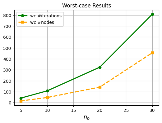
Figure 2: Worst-case number of iterations and B&B nodes as a function of $n_{b}$ for random mp-experiments.

To illustrate the impact of parallel algorithms on computation time, Fig. 3 presents the speed-up factor, defined as $\frac{t^{s}}{t^{p}}$, where $t^{s}$ and $t^{p}$ denote the CPU execution times of the serial and parallel certification algorithms, respectively. These results are based on experiments conducted on supercomputers for random MILPs with $n_{b}=30$, presented as a function of the number of employed workers. For reference, the ideal linear speed-up is also shown.

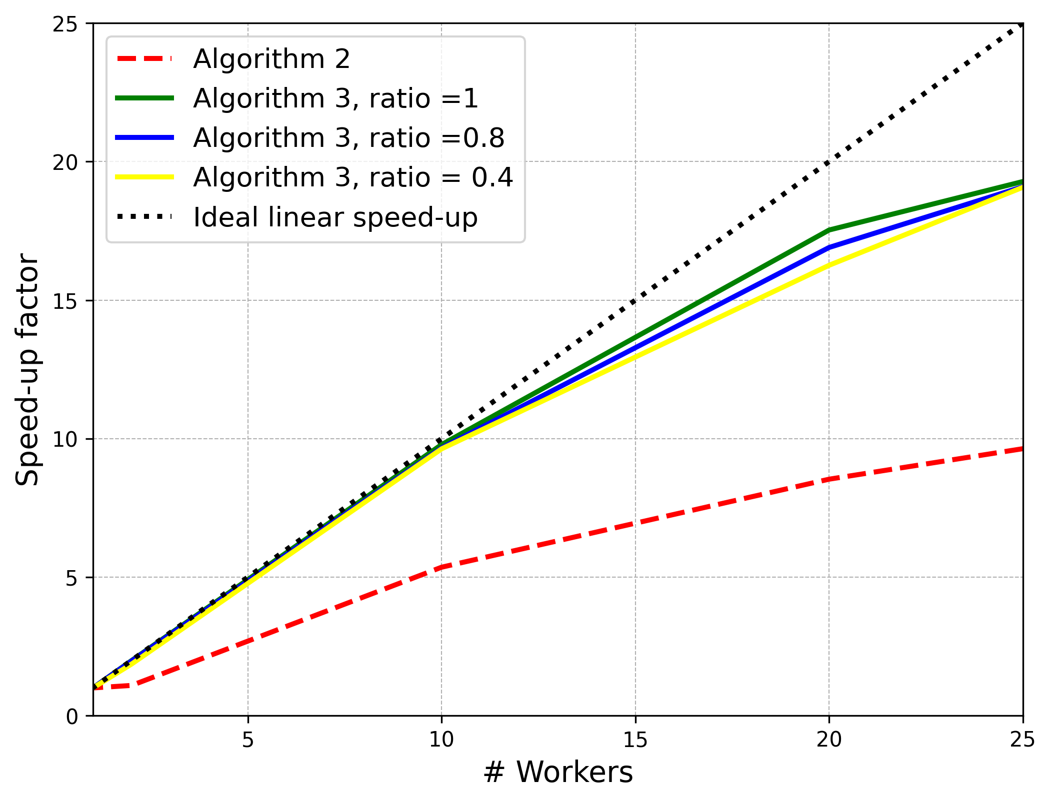
Figure 3: Speed-up factor of Algorithm 2 (dashed red line) alongside the speed-up factor of Algorithm 3 for three different ratios (solid lines), compared to the ideal linear speed-up (dotted black line), as a function of the number of workers for random experiments.

From Fig. 3, it is clear that the parallel algorithms significantly accelerate computation. For a larger number of workers, however, the speed-up deviates from the ideal trend, highlighting the emergence of communication overhead. In particular, the speed-up factor closely follows the ideal linear trend for fewer workers when using Algorithm 3 (and its variant, Algorithm 4). Furthermore, larger distribution ratios can lead to more consistent speed-up. Algorithm 2, on the other hand, provides a moderate improvement over Algorithm 1 and achieves a lower speed-up compared to Algorithm 3. This is primarily due to the extra regions generated from the initial artificial partitioning, which increase the computational workload (see Fig. 5 (b) and (d)). These results emphasize the importance of dynamic workload distribution to fully leverage the problem structure and improve performance.

To illustrate the reduction in peak resource consumption achieved by Algorithm 4, Fig. 4 shows the number of tuples stored in $\mathcal{S}_{d}$ (i.e., $|\mathcal{S}_{d}|$) in the master over the course of Algorithms 3 and 4. In this experiment, the solveCert subroutine was paused when a maximum of 100 regions was generated. Algorithm 4 generally requires more outer iterations, since in certain iterations, only the cut conditions are evaluated (see Steps 8–9). In this experiment, the master in Algorithm 4 performed about 100 more outer iterations than Algorithm 3, during which $|\mathcal{S}_{d}|=0$ for Algorithm 3. While the total execution time for both algorithms was approximately the same, Algorithm 4 exhibited lower memory consumption. This is reflected in the maximum number of tuples stored in $\mathcal{S}_{d}$, which is around 100 for Algorithm 4, compared to approximately 1000 for Algorithm 3. Notably, the peaks in Fig. 4 correspond to outer iterations in which a relaxation was certified.

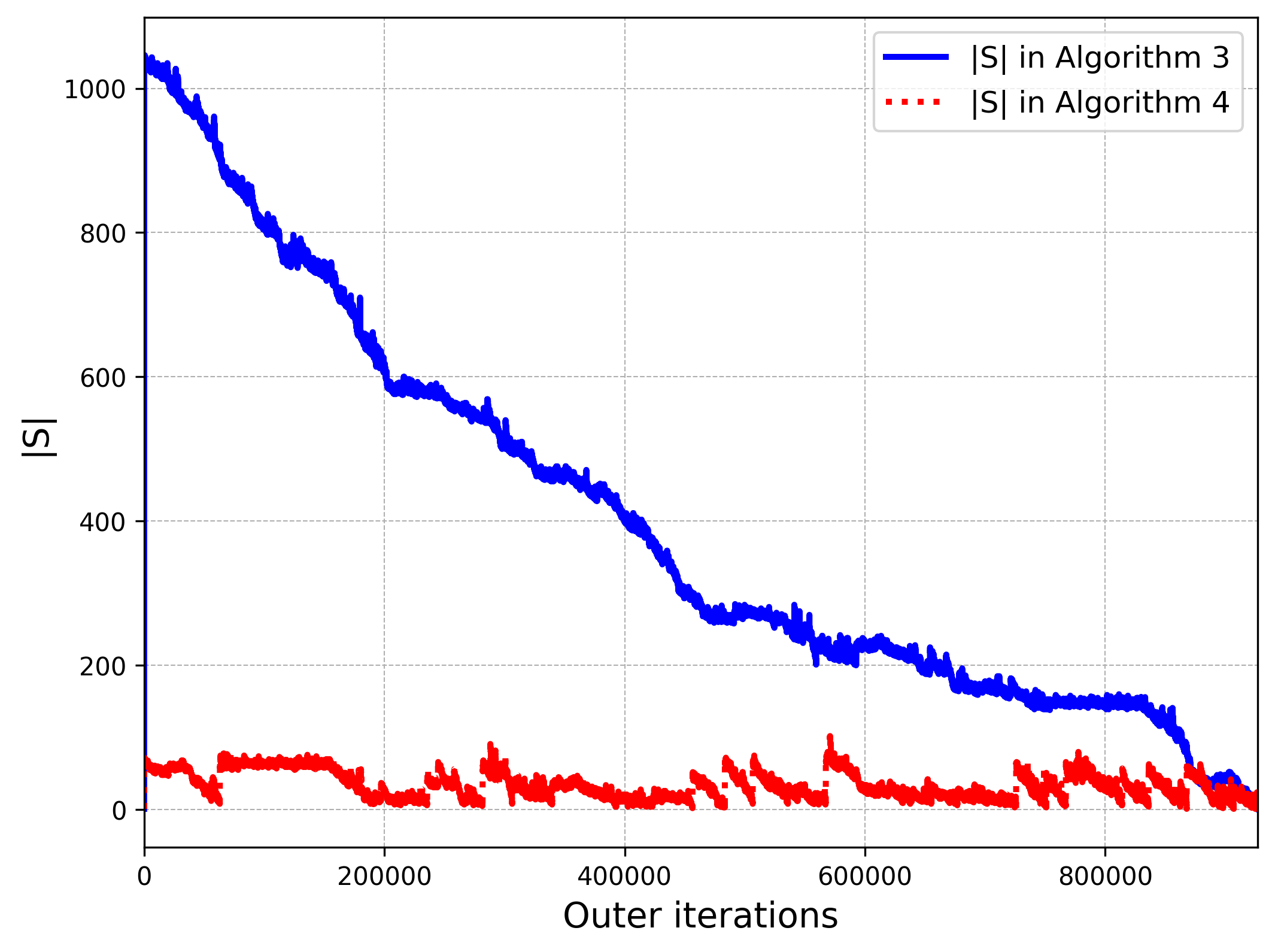
Figure 4: The number of tuples stored in $\mathcal{S}_{d}$ in the master during Algorithms 3 (solid blue line) and 4 (dotted red line).

Finally, to provide visual insights into the results of Algorithms 2 and 3, Fig. 5 presents a two-dimensional slice of the resulting partition for two randomly generated problems, with $n_{b}=10$ in (a) and (b), and $n_{b}=20$ in (c) and (d). Specifically, Fig. 5 (a) and (c) show the final regions generated using Algorithm 3, resulting in 36 and 2510 regions, respectively, identically to the final partitioning when applying Algorithm 1. Similarly, Fig. 5 (b) and (d) illustrate the partitions obtained using Algorithm 2, yielding 69 and 2696 regions, respectively. The additional partitions in Fig. 5 (b) and (d) arise from the initial artificial partitioning introduced in Algorithm 2.

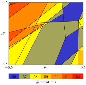
(a)

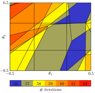
(b)

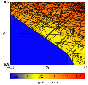
(c)

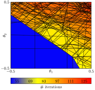
(d)

Figure 5: Resulting parameter space partitions for two randomly generated examples, determined using Algorithm 3 in (a) and (c), and Algorithm 2 in (b) and (d). Results are shown for $n_{b}=10$ in (a) and (b), and $n_{b}=20$ in (c) and (d).

VI-B MPC application

We now apply the proposed methods to a hybrid MPC problem involving a linearized inverted pendulum on a cart, constrained by a wall, as used in, e.g., [20, 13] (see Fig.6). The objective is to stabilize the pendulum at the origin ($z_{1}=0$) while keeping it upright ($z_{2}=0$). The control inputs consist of a force applied to the cart ($u_{1}$) and a contact force from wall interaction ($u_{2}$), introducing binary variables into the model. The state and input constraints follow those in[20, 13]. The hybrid MPC controller employs a quadratic performance measure with a prediction/control horizon of $N$. The system’s initial state vector serves as the parameter vector $\theta$ in the multi-parametric setting, with the parameter set determined by state constraints. The resulting mp-MIQP, formulated following [4], includes $n=4N$ decision variables, of which $n_{b}=2N$ are binary. The weights matrices and dynamics are consistent with those in [20]. For further details, see [20].

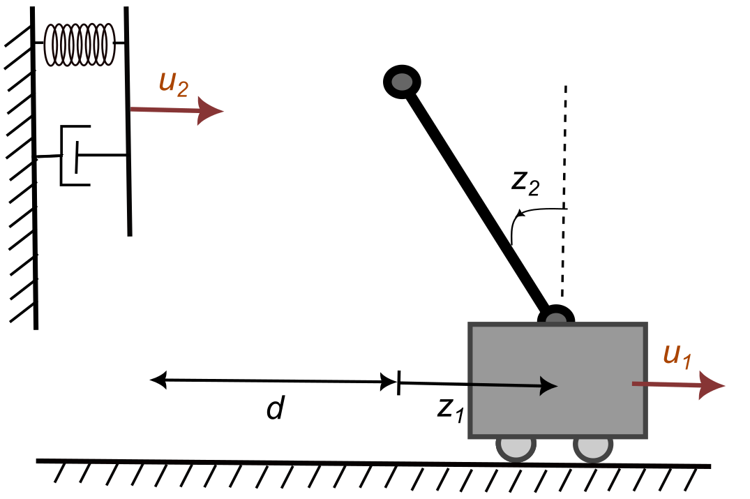
Figure 6: Regulating the inverted pendulum on a cart with contact forces.

Table I summarizes the complexity certification results for the (serial) certification Algorithm 1 and the parallel certification Algorithms 2 and 3 executed using $10$ workers, as a function of the prediction horizon $N$. The table reports the number of constraints ($m$), the worst-case computational complexity in terms of iterations ($\kappa^{I}_{\text{wc}}$) and B&B nodes ($\kappa^{N}_{\text{wc}}$), along with the CPU time required for certification (in seconds). The results highlight the impact of parallelization in reducing computational time. Specifically, as the problem size increases (i.e., as $N$ grows), the parallel algorithms outperform the serial one in terms of certification time, while maintaining correct results.

TABLE I: The number of constraints ($m$) in the resulting mp-MIQPs for the inverted pendulum example, along with worst-case complexity results and the computation time of the Julia implementation for Algorithm 1 ($t^{\text{ser}}$), Algorithm 2 ($t^{\text{stat}}$), and Algorithm 3 ($t^{\text{dyn}}$) across different prediction horizons ($N$).

prob. dim.		wc. complexity		cert. time [sec]
$N$	$m$	$\kappa^{I}_{\text{wc}}$	$\kappa^{N}_{\text{wc}}$	$t^{\text{ser}}$	$t^{\text{stat}}$	$t^{\text{dyn}}$
1	19	9	4	1.4	0.93	0.48
2	38	22	8	6.2	3.2	1.9
3	57	76	47	44.6	20.3	11.1
4	76	134	68	122	46.4	30.1
5	95	198	76	635	201.3	119.4
6	114	250	78	1311.6	326.9	212.7

VII Conclusion

This paper presents parallel versions of the complexity certification framework for B&B-based MILP and MIQP solvers applied to the family of mp-MILPs and mp-MIQPs, extending its applicability to larger and more challenging problem instances. The proposed algorithms employ both static and dynamic domain decomposition to distribute computational workloads across available processing resources. To address the challenge of peak memory consumption in computationally demanding problems, two complementary strategies are introduced and integrated into the parallel algorithms. These enhancements improve the scalability of the method, even for more memory-intensive problems. The parallel algorithms enable the use of HPC resources, facilitating the certification of larger and more complex problem instances. Numerical experiments demonstrate significant reductions in computation time while preserving the correctness of the certification results. Future work will focus on further refining the implementation, including parallelizing the solveCert subroutine to further distribute the computational workload.

References

- [1] V. Dua, N. A. Bozinis, and E. N. Pistikopoulos, “A multiparametric programming approach for mixed-integer quadratic engineering problems,” Computers & Chemical Engineering, vol. 26, no. 4-5, pp. 715–733, 2002.
- [2] F. Borrelli, M. Baotić, A. Bemporad, and M. Morari, “Dynamic programming for constrained optimal control of discrete-time linear hybrid systems,” Automatica, vol. 41, no. 10, pp. 1709–1721, 2005.
- [3] F. Borrelli, A. Bemporad, and M. Morari, Predictive control for linear and hybrid systems. Cambridge University Press, 2017.
- [4] A. Bemporad, F. Borrelli, M. Morari et al., “Model predictive control based on linear programming – the explicit solution,” IEEE Transactions on Automatic Control, vol. 47, no. 12, pp. 1974–1985, 2002.
- [5] V. Dua and E. N. Pistikopoulos, “An algorithm for the solution of multiparametric mixed integer linear programming problems,” Annals of Operations Research, vol. 99, no. 1, pp. 123–139, 2000.
- [6] M. N. Zeilinger, C. N. Jones, and M. Morari, “Real-time suboptimal model predictive control using a combination of explicit MPC and online optimization,” IEEE Transactions on Automatic Control, vol. 56, no. 7, pp. 1524–1534, 2011.
- [7] G. Cimini and A. Bemporad, “Exact complexity certification of active-set methods for quadratic programming,” IEEE Transactions on Automatic Control, vol. 62, no. 12, pp. 6094–6109, 2017.
- [8] D. Arnström and D. Axehill, “A unifying complexity certification framework for active-set methods for convex quadratic programming,” IEEE Transactions on Automatic Control, vol. 67, no. 6, pp. 2758–2770, 2022.
- [9] S. Shoja, D. Arnström, and D. Axehill, “Exact complexity certification of a standard branch and bound method for mixed-integer linear programming,” in Proceedings of the 61st IEEE Conference on Decision and Control (CDC), 2022, pp. 6298–6305.
- [10] S. Shoja and D. Axehill, “Exact complexity certification of suboptimal branch-and-bound algorithms for mixed-integer linear programming,” IFAC-PapersOnLine, vol. 56, no. 2, pp. 7428–7435, 2023.
- [11] D. Axehill and M. Morari, “Improved complexity analysis of branch and bound for hybrid MPC,” in Proceedings of the 49th IEEE Conference on Decision and Control (CDC). IEEE, 2010, pp. 4216–4222.
- [12] S. Shoja, D. Arnström, and D. Axehill, “Overall complexity certification of a standard branch and bound method for mixed-integer quadratic programming,” in Proceedings of 2022 American Control Conference (ACC), 2022, pp. 4957–4964.
- [13] ——, “A unifying complexity certification framework of standard branch-and-bound algorithms for mixed-integer linear and quadratic programming,” Submitted., 2025.
- [14] G. A. Constantinides, “Tutorial paper: Parallel architectures for model predictive control,” in 2009 European Control Conference (ECC). IEEE, 2009, pp. 138–143.
- [15] D. Bertsekas and J. Tsitsiklis, Parallel and distributed computation: numerical methods. Athena Scientific, 2015.
- [16] T. Ralphs, Y. Shinano, T. Berthold, and T. Koch, “Parallel solvers for mixed integer linear programming,” Tech. Rep. 16-74, ZIB, Takustr.7, 14195 Berlin, 2016.
- [17] L. A. Wolsey, Integer programming. John Wiley & Sons, 2020.
- [18] J. Nocedal and S. Wright, Numerical optimization. Springer Science & Business Media, 2006.
- [19] National Supercomputer Centre. [Online]. Available: https://www.nsc.liu.se/
- [20] T. Marcucci and R. Tedrake, “Warm start of mixed-integer programs for model predictive control of hybrid systems,” IEEE Transactions on Automatic Control, vol. 66, no. 6, pp. 2433–2448, 2020.