Truthful Elicitation of Imprecise Forecasts

Abstract

The quality of probabilistic forecasts is crucial for decision-making under uncertainty. While proper scoring rules incentivize truthful reporting of precise forecasts, they fall short when forecasters face epistemic uncertainty about their beliefs, limiting their use in safety-critical domains where decision-makers (DMs) prioritize proper uncertainty management. To address this, we propose a framework for scoring imprecise forecasts—forecasts given as a set of beliefs. Despite existing impossibility results for deterministic scoring rules, we enable truthful elicitation by drawing connection to social choice theory and introducing a two-way communication framework where DMs first share their aggregation rules (e.g., averaging or min-max) used in downstream decisions for resolving forecast ambiguity. This, in turn, helps forecasters resolve indecision during elicitation. We further show that truthful elicitation of imprecise forecasts is achievable using proper scoring rules randomized over the aggregation procedure. Our approach allows DM to elicit and integrate the forecaster’s epistemic uncertainty into their decision-making process, thus improving credibility.

Keywords: Imprecise Probability, Scoring Rules, Elicitation

1 Introduction

Probabilistic forecasting is a powerful tool for decision-making under uncertainty with diverse applications ranging from energy demand forecasting (pinson2012evaluating; pinson2013wind) and credit risk assessment (rindt2022survival; yanagisawa2023proper) to machine learning (ML) (gneiting2007strictly) and large language models (LLMs) (shao2024language; wu2024elicitationgpt). Proper scoring rules serve as fundamental tools for evaluating the quality of probabilistic forecasts (brier1950verification; murphy1988decomposition; gneiting2007strictly). They also serve as a backbone for eliciting other distributional properties such as their moments. (frongillo2014general). By assigning numerical scores based on the reported forecast and the realized outcome, these rules incentivize truthful reporting, i.e., any deviation from the forecaster’s true beliefs would result in suboptimal scores. Beyond their applications in statistics, proper scoring rules have a deep connection with mechanism design, a sub-field of economics. When used as a payment mechanism, they ensure that the agents have no incentive to lie, a property known as incentive compatibility (myerson1981optimal).

Traditionally, scoring rules operate under the assumption that forecasters possess a precise probabilistic belief about some uncertain event. They are designed to reward the forecasters whose forecasts reflect their true precise beliefs (savage1971elicitation; gneiting_probabilistic_2014). For example, in weather forecasting (brier1950verification) a forecaster who believes there is a 60% chance of rain tomorrow should ideally report 60% as their forecast. However, in many real-world scenarios, forecasters face significant ambiguity due to the inherent complexity of atmospheric systems, coupled with limited data and model resolution, which introduce substantial imprecision (wilks2011statistical). It is thus plausible for forecasters to report imprecise probability assessments in these scenarios; for example, the chance of rain tomorrow may be assessed within the interval $[50\%,70\%]$. Importantly, classical proper scoring rules built for precise forecasts cannot account for such additional uncertainty (konek2015).

Under the context of machine learning, imprecise forecasting is closely related to the concept of out-of-distribution (OOD) generalization (muandet_domain_2013; Wang21:DG-Review; Zhou21:DG-Review). In standard supervised learning, where training and test data are assumed to be independent and identically distributed (i.i.d.), the predictive model reflects the learner’s precise belief about the data generating process. However, in OOD generalization—where multiple training datasets are observed, and the test data may not be i.i.d. with the training data—singh2024domain argue that the notion of generalization (e.g., average-case or worst-case optimization strategy) should be determined by the model’s end user, also referred to as the decision-maker (DM). When direct interaction between the learner and the DM is not possible, singh2024domain propose an imprecise learning algorithm that trains a portfolio of predictors (forecasts) in advance, which are then provided to the DM. In contrast, for practical scenarios where the learner and DM can communicate, eliciting precise forecasts is straightforward using classical scoring rules. However, eliciting imprecise forecasts remains challenging due to the lack of suitable imprecise scoring rules. This gap motivates us to design appropriate imprecise scoring rules that are applicable beyond machine learning contexts.

In these scenarios, the key challenge to designing an appropriate scoring mechanism arises from the forecaster’s epistemic uncertainty. This challenge has led to several impossibility theorems for strictly proper imprecise scoring rules (seidenfeld2012; mayo2015accuracy; schoenfield2017accuracy). However, these works focus solely on eliciting imprecise forecasts from the forecaster, overlooking the fact that probabilistic forecasts are typically used by downstream DMs, making elicitation rarely the sole objective. Without input from the DMs during elicitation, forecasters must rely solely on their imprecise beliefs, which contain inherent ambiguity. This often leads to indecision during elicitation—a key factor behind the impossibility results observed in prior work. Recently, frohlich2024scoring explored imprecise scoring rules involving DMs, but their analysis focused only on min-max (pessimistic) decision-making and lacked formal discussion of the DM’s role. More broadly, indecision can be resolved through subjective choices beyond the min-max rule. However, it cannot be resolved by forecasters independently without eliminating their epistemic uncertainty. We argue that the DM must actively assist forecasters in navigating indecision by communicating their subjective preferences.

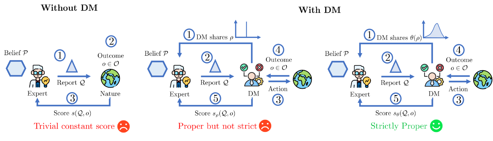
Figure 1: We consider scenarios where the expert may possess imprecise belief over the outcome $o\in{\mathcal{O}}$, represented as a credal set ${\mathcal{P}}\subseteq\Delta({\mathcal{O}})$. The goal is to construct a strictly proper imprecise scoring rule $s({\mathcal{Q}},o)$ to incentivise a truthful report ${\mathcal{Q}}={\mathcal{P}}$. The leftmost figure illustrates the direct extension of precise scoring rules to the imprecise setting. Scoring rules in precise settings, however, do not involve the downstream decision-maker (DM) in the elicitation process. In this work, we show that truthful elicitation of imprecise forecasts requires the DM to share their knowledge of the aggregation rule $\rho$ used in decision making with the expert (middle). To avoid strategic manipulation by the expert, the rightmost figure depicts the proposed framework in which the DM shares only a distribution $\theta(\rho)$ over aggregation rules. This allows us to construct a strictly proper imprecise scoring rule, $s_{\theta}$.

Our contributions. To address this challenge, we propose a novel setup for scoring imprecise forecasts where we consider a DM as an additional agent, who actively guides the forecaster in resolving indecision during elicitation. Our contributions are summarized as follows:

• We show that, without communication between the DM and the forecaster, we recover prior impossibility results.

• We formalize DM-forecaster communication using aggregation rules from social choice theory (arrow2012social) and generalize tailored scoring rules  (johnstone2011tailored) to accommodate these aggregations.

• We analyze the connection between axiomatic properties of aggregation rules from the social choice perspective and their impact on both truthful elicitation from the forecaster and the DM’s decision-making process.

• By restricting to strategic communication, specifically by sharing only a distribution over aggregation rules, we propose a novel randomized tailored scoring rule that is strictly proper for imprecise forecasts.

The rest of the paper is organized as follows. Section 2 introduces proper scoring rules and imprecise probabilities. Section 3 then formalizes the notion of an imprecise forecaster and outlines decision-making for the forecaster and DM. Next, Section 4 explores imprecise scoring rules, first without communication and then with aggregation. Section 5 presents strictly proper scoring rules for imprecise forecasts, while Section 6 reviews prior work. Finally, Section 7 concludes with a discussion of future directions.

2 Preliminaries

This section introduces proper scoring rules, imprecise probabilities and credal sets. We begin by establishing the notation. Let $({\mathcal{O}},{\mathcal{F}})$ be a measurable space where ${\mathcal{O}}$ is a nonempty continuous set of possible outcomes (or states of nature) and ${\mathcal{F}}$ the corresponding sigma-algebra. An uncertain event is denoted by a random variable $\bm{X}:{\mathcal{O}}\rightarrow\mathbb{R}$ and $\Delta({\mathcal{O}})$ denotes the set of plausible probability distributions on ${\mathcal{O}}$. Our framework involves two agents: a forecaster and a decision-maker (DM), each with an associated utility functions $u:{\mathcal{X}}\times{\mathcal{O}}\rightarrow\mathbb{R}$, where ${\mathcal{X}}$ represents the input space relevant to the agent’s utility. Since we often refer to specific outcomes $o\in\mathcal{O}$, we assume $\bm{X}$ to be the identify function when discussing expected utilities. Thus, for some $x\in\mathcal{X}$, th agent’s expected utility under a distribution $p$ is expressed as: $\mathbb{E}_{\bm{X}\sim p}[\bm{X}_{x}(o)]$, where $\bm{X}_{x}(o):=u(x,o)$ is used as shorthand. Additionally, ${\mathcal{H}}$ denotes Hilbert space.

2.1 Precise Scoring Rules

Scoring rules incentivize an expert to truthfully report their probability assessments of an uncertain event (winkler1967quantification; brier1950verification). Specifically, a scoring rule $s:\Delta({\mathcal{O}})\times{\mathcal{O}}\rightarrow\mathbb{R}$ assigns a score of $s(q,o)$ to an expert with a forecast $q$ when an outcome $o$ happens.

Definition 2.1.

A forecaster is precise if their true belief can be expressed as a probability distribution $p\in\Delta({\mathcal{O}})$.

Since classical proper scoring rules focus on truthful reporting and evaluation of precise forecasts, we refer them as precise scoring rules. A precise scoring rule is regular if $s(q,o)\in\mathbb{R}$ for all $o\in{\mathcal{O}}$ and $s(q,o)=-\infty$ only if $q(o)=0$. A regular scoring rule disincentivises strong predictions about the impossibility of an event.

Definition 2.2 (Expected Utility of Expert).

Precise scoring rules implicitly assume that the expert is an expected utility-maximising agent. Therefore for an expert with true belief $p$, utility of reporting forecast $q$ is

$$u_{p}(q)=\mathbb{E}_{o\sim p}[s(q,o)]$$ (1)

We now define a sub-class of regular precise scoring rules, known as strictly proper precise scoring rules that incentivize truthful reporting of the expert’s belief.

Definition 2.3 (Strictly Proper Precise Scoring Rule).

A regular precise scoring rule $s:\Delta({\mathcal{O}})\times{\mathcal{O}}\rightarrow\mathbb{R}\cup\{-\infty\}$ is strictly proper if the expert’s true belief $p\in\Delta({\mathcal{O}})$ uniquely maximizes their expected utility, i.e., for all $p,q\in\Delta({\mathcal{O}})$,

$$\mathbb{E}_{o\sim p}[s(p,o)]>\mathbb{E}_{o\sim p}[s(q,o)]$$ (2)

Some examples of strictly proper precise scoring rules are, logarithmic scoring rule $s(q,o)=a_{o}+b\text{ }\log(q(o))$ and quadratic scoring rule $s(q,o)=a_{o}+b(2q(o)-\mathbb{E}_{o\sim q}[q(o)])$ with $b\in\mathbb{R}_{+}$ and $a_{o}\in\mathbb{R}$ as arbitrary parameters. Proper precise scoring rules are closely related to convexity and can be characterized using convex functions as shown in  mccarthy1956measures; savage1971elicitation; gneiting2007strictly.

Theorem 2.4 (gneiting2007strictly).

A regular scoring rule $s$ is (strictly) proper if and only if

$$s(q,o)=G(q)-\int G^{\prime}(q)dq+G^{\prime}(q)(o)$$ (3)

where $G:\Delta({\mathcal{O}})\rightarrow\mathbb{R}$ is a (strictly) convex function and $G^{\prime}(q)$ is a subgradient of $G$ at point $q$ and $G^{\prime}(q)(o)$ is the value of gradient at outcome $o$.

An implication of Theorem 2.4 is that with this characterisation of the scoring rule $s$, we can interpret $G$ as the corresponding maximum expected score  (frongillo2014general). The derivation of $G$ as the expected score is included in the appendix A.1 for completeness.

2.2 Imprecise Probabilities and Credal Sets

Standard probability theory assigns a unique numerical value to each event, whereas imprecise probabilities allow for a range of plausible values to represent uncertainty in the presence of limited or ambiguous information. One common approach to modelling such uncertainty is via credal sets. A credal set ${\mathcal{P}}$ is defined as a subset of the plausible probability distributions over a given outcome space ${\mathcal{O}}$, i.e.,

$${\mathcal{P}}\subseteq\Delta({\mathcal{O}})=\left\{p:{\mathcal{O}}\to[0,1]\mid\int dp(o)=1\right\}.$$

It is important to note that while many authors assume that ${\mathcal{P}}$ is convex (and often closed) to ensure consistency with rational decision-making (gajdos2004decision; troffaes2007decision) and to satisfy coherence (definetti1974theory; walley1991statistical), the definition itself does not require ${\mathcal{P}}$ to be the convex hull. Rather, ${\mathcal{P}}$ is directly specified as a set of probability measures representing the range of plausible beliefs about the state of nature (walley1991statistical; augustin2014introduction). For clarity, we denote the credal set that is the convex hull of probabilities with ${\text{co}}({\mathcal{P}})$ and the extreme points of such convex hull as ${\text{ext}}({\mathcal{P}})$. Generalizing classical scoring rules to accommodate imprecise probabilities involves adapting the classic framework to account for all the distributions in the credal sets. This will ensure the generalized scoring mechanism’s validity for non-singleton sets of probabilities.

3 A Unifying Decision-making Framework for DM and Forecaster

In this work, we consider scenarios where an agent is tasked with selecting an input $x$ from a finite space of inputs ${\mathcal{X}}:=\{x_{1},\ldots,x_{n}\}$. Agent’s choice of input $x\in{\mathcal{X}}$ and outcome of uncertain event $o\in{\mathcal{O}}$ quantify the utility $u(x,o)$ obtained by the agent. In the case of a precise forecaster, ${\mathcal{X}}:=\Delta({\mathcal{O}})$ and the equation 1 shows how the precise score $u(x,o):=s(p,o)$ acts as a utility for the forecaster, underlining the decision-making aspect within elicitation. From the DM’s perspective, ${\mathcal{X}}:={\mathcal{A}}$ where ${\mathcal{A}}:=\{a_{1},\dots,a_{m}\}$ denotes the finite space of actions which DM can choose from. Depending upon the outcome $o\in{\mathcal{O}}$, the DM obtains $u(x,o):=u(a,o)$ as the utility.

3.1 Decision-Making with Forecasts

There exists a crucial difference between decision-making with imprecise forecasts v.s. precise forecasts. In the case of precise forecasts, the agent (forecaster or DM) has (via belief or report) a $p\in\Delta({\mathcal{O}})$. Using $p$ allows them to define a complete preference relation $\succeq_{p}$ over ${\mathcal{X}}$ based on several well-established rationality frameworks (von2007theory; savage1972foundations). Thereby, allowing the agent to select the corresponding best input $x^{*}$. This $x^{*}$ represents the best forecast to report in the case of a precise forecaster and the best action to take in the case of DM. However, in scenarios where the belief (or obtained report) for an agent is a credal set ${\mathcal{P}}$, the preference relation ($\succeq_{{\mathcal{P}}}$) obtained on ${\mathcal{X}}$ using ${\mathcal{P}}$ is unclear. In this case, a natural way to define $\succeq_{{\mathcal{P}}}$ is based on the idea of dominance.

Definition 3.1.

Consider a credal set ${\mathcal{P}}$, then the corresponding preference relation $\succeq_{{\mathcal{P}}}$ over ${\mathcal{X}}$ for a VNM rational (von2007theory) agent can be defined as follows, for all $x,x^{\prime}\in{\mathcal{X}}$,

$$x\succeq_{{\mathcal{P}}}x^{\prime}\quad\text{iff}\quad\mathbb{E}_{p}[u(x,o)]\geq\mathbb{E}_{p}[u(x^{\prime},o)]\quad\forall p\in{\mathcal{P}}$$

Unless the reported credal set ${\mathcal{P}}$ is implicitly a precise forecast of type $\{p\in\Delta({\mathcal{O}})\}$, the preference relation $\succeq_{{\mathcal{P}}}$ is a partial order over ${\mathcal{X}}$. The partial order $\succeq_{{\mathcal{P}}}$ can be incomplete, since there can be a pair of inputs $x,x^{\prime}\in{\mathcal{X}}$ such that $x^{\prime}\not\succeq_{{\mathcal{P}}}x$ and $x\not\succeq_{{\mathcal{P}}}x^{\prime}$. In other words, $x$ and $x^{\prime}$ are incomparable. This can result in indecision for the agent. This means that both the forecaster and the DM face indecision when solely relying on the credal set for their respective tasks (elicitation or decision-making).

3.2 Imprecise Forecaster

Our work focuses on analyzing scoring rules in scenarios where the forecaster may be imprecise. Specifically, we formalise the notion of an imprecise forecaster and their truthfulness below.

Definition 3.2.

A forecaster is imprecise if their true belief can be expressed as a set of probability distributions ${\mathcal{P}}\subseteq\Delta({\mathcal{O}})$. A report ${\mathcal{Q}}\subseteq\Delta({\mathcal{O}})$ is called an imprecise forecast, which implicitly includes precise forecasts ${\mathcal{Q}}=\{q\}$ for some $q\in\Delta({\mathcal{O}})$.

Definition˜3.2 generalizes the precise setting as it allows the forecaster to express their (partial) ignorance by reporting both aleatoric uncertainties (as elements in the set) and epistemic uncertainties (as the set itself) (hullermeier_aleatoric_2021). This subsumes both scenarios where the forecaster’s belief is truly imprecise, e.g., the probability that it will rain tomorrow is $[0.6,0.8]$, and where their belief is calibrated with respect to multiple sources of potentially conflicting information, e.g., the estimated probability based on data from multiple weather stations. Moreover, this can also be interpreted as a “collective” report obtained from multiple (potentially conflicting) precise forecasters.

Imprecise probability scoring rules can be defined analogously to precise scoring rules as follows.

Definition 3.3.

(Imprecise Probability Scoring Rule) An imprecise probability (IP) scoring rule $s:2^{\Delta({\mathcal{O}})}\times{\mathcal{O}}\rightarrow\mathbb{R}\cup\{-\infty\}$ assigns a score of $s({\mathcal{Q}},o)$ to a report ${\mathcal{Q}}\subseteq\Delta({\mathcal{O}})$ when the outcome $o\in{\mathcal{O}}$ is realized.

Analogous to precise setting, an IP scoring rule is regular if $s({\mathcal{Q}},o)\in\mathbb{R}$ for all $o\in{\mathcal{O}}$, except if $q(o)=0$ for all $q\in{\mathcal{Q}}$, then $s({\mathcal{Q}},o)=-\infty$. To define regularity analogous to the precise setting we consider for all $q\in{\mathcal{Q}}$, since otherwise reporting vacuous set $\Delta({\mathcal{O}})$ or other imprecise sets will have $-\infty$ as an incentive. Thereby discouraging the forecaster from reporting their epistemic uncertainty. The score $s({\mathcal{Q}},o)$ obtained by the forecaster induces a corresponding set of utilities $\bm{V}^{\mathcal{P}}({\mathcal{Q}})$ for the forecaster with an imprecise belief ${\mathcal{P}}$, representing the expected utility of the imprecise score with respect to every precise distribution within their belief ${\mathcal{P}}$. We define this utility set as follows:

$$\bm{V}^{\mathcal{P}}({\mathcal{Q}})=\{\mathbb{E}_{p}[s({\mathcal{Q}},o)]\}_{p\in{\mathcal{P}}}$$ (4)

From the forecaster’s perspective this collection of expected utility functions $\bm{V}^{\mathcal{P}}:2^{\Delta({\mathcal{O}})}\rightarrow\mathbb{R}^{|{\mathcal{P}}|}$, for each report ${\mathcal{Q}}$ result in a range of plausible expected utility, i.e.,

$$\text{im}(\bm{V}^{{\mathcal{P}}}({\mathcal{Q}}))=\Bigg{[}\inf_{p\in{\mathcal{P}}}\mathbb{E}_{p}[s({\mathcal{Q}},o)],\sup_{p\in{\mathcal{P}}}\mathbb{E}_{p}[s({\mathcal{Q}},o)]\Bigg{]}$$ (5)

where im is the image or the range of the forecaster’s minimum and maximum expected utility for a given forecast. While the equivalence of two precise distributions is natural i.e. whether two distributions $p=q$ or not. The equivalence of two imprecise beliefs is not obvious as they are sets of distributions. We now define the equivalence of two beliefs ${\mathcal{P}},{\mathcal{P}}^{\prime}$ in the context of elicitation as follows

Definition 3.4.

(Equivalence of imprecise beliefs) Two beliefs ${\mathcal{P}},{\mathcal{P}}^{\prime}\subseteq\Delta({\mathcal{O}})$ are considered equivalent, denoted as ${\mathcal{P}}\simeq{\mathcal{P}}^{\prime}$, if for all IP scoring rules $s$ and forecasts ${\mathcal{Q}}\subseteq\Delta({\mathcal{O}})$, we have $\text{im}(\bm{V}^{{\mathcal{P}}}({\mathcal{Q}}))=\text{im}(\bm{V}^{{\mathcal{P}}^{\prime}}({\mathcal{Q}}))$.

Intuitively, we define the equivalence of two imprecise forecasts based on the premise that they do not differ in the range of plausible expected utilities for any scoring rule $s$ and reported imprecise forecast ${\mathcal{Q}}$, i.e. the decision-making induced by two imprecise beliefs ${\mathcal{P}}$ and ${\mathcal{P}}^{\prime}$ is same under all scenarios. We now show that Definition˜3.4 when used for precise forecasts does not change the classic notion of equivalence.

Proposition 3.5.

For all $p,q\in\Delta({\mathcal{O}})$, $\{p\}\simeq\{q\}$ iff $p=q$.

With Proposition 3.5, we establish that Definition˜3.4 generalises from the notion of equivalence of precise forecasts, i.e. distributions to imprecise forecasts. We can also characterize the equivalence of two imprecise forecasts as the equivalence of their corresponding credal sets.

Proposition 3.6.

For imprecise forecasts ${\mathcal{P}},{\mathcal{P}}^{\prime}\subseteq\Delta({\mathcal{O}})$, ${\mathcal{P}}\simeq{\mathcal{P}}^{\prime}$ if and only if $co({\mathcal{P}})=co({\mathcal{P}}^{\prime})$.

It has previously been shown that two sets of distributions must be credal sets to induce the same rational decision-making behaviour (troffaes2007decision; huntley2014decision; troffaes2014lower). Definition˜3.4 defines the equivalence of two imprecise beliefs w.r.t elicitation and Proposition 3.6 establishes its equivalence to rational decision making. This allows us to consider elicitation as a decision-making task for the forecaster. As a consequence of Proposition  3.6, even though a forecaster outputs a set of probability distributions ${\mathcal{P}}$. We restrict our focus to evaluating a credal set of forecasts $co({\mathcal{P}})$. Henceforth, with a slight abuse of notation, we will use ${\mathcal{P}}$ to represent $co({\mathcal{P}})$.

Definition 3.7.

(Truthfulness of Imprecise Forecaster) Let ${\mathcal{P}}\subseteq\Delta({\mathcal{O}})$ be the true belief of an imprecise forecaster. A report ${\mathcal{Q}}\subseteq\Delta({\mathcal{O}})$ is truthful if ${\mathcal{Q}}\simeq{\mathcal{P}}$.

Definition˜3.7 generalizes the concept of truthfulness in the precise setting. An imprecise forecaster who reports their true belief is considered truthful. For instance, if the forecaster believes the probability of rain tomorrow lies within the interval $[0.6,0.8]$, then they must report their actual epistemic uncertainty by reporting the interval $[0.6,0.8]$.

4 Proper IP Scoring Rules

In this section, we introduce proper imprecise scoring rules, i.e., scores that incentivize the truthful elicitation of an imprecise forecaster according to Definition˜3.7. We start by focusing only on the elicitation of the imprecise forecaster without any communication from the DM. The following definition clarifies what it means for an imprecise scoring rule to be (strictly) proper, which naturally generalises Definition˜3.1 from the forecaster’s perspective.

Definition 4.1.

An imprecise scoring rule is (strictly) proper if for all credal sets ${\mathcal{P}},{\mathcal{Q}}\subseteq\Delta({\mathcal{O}})$, the forecaster with an imprecise belief ${\mathcal{P}}\not\simeq{\mathcal{Q}}$ (strictly) prefers ${\mathcal{P}}$ over ${\mathcal{Q}}$, i.e., ${\mathcal{P}}\succeq_{{\mathcal{P}}}{\mathcal{Q}}$. The preference relation $\succeq_{{\mathcal{P}}}$ is described by the (strict) dominance of $\bm{V}^{{\mathcal{P}}}({\mathcal{P}})$ over $\bm{V}^{{\mathcal{P}}}({\mathcal{Q}})$, i.e.,

$$\mathbb{E}_{p}[s({\mathcal{P}},o)]\geq\mathbb{E}_{p}[s({\mathcal{Q}},o)]\quad\text{for all }p\in{\mathcal{P}},$$

for strict dominance, at least one $\geq$ has to be strictly greater.

We define strict properness of an imprecise scoring rule in Definition˜4.1 using dominance since it preserves the main idea behind strictly proper scoring rules in the precise setting, i.e. to incentivise the forecaster to be truthful. A strictly proper IP scoring rule incentivises the imprecise forecaster to be truthful according to Definition˜3.7.

Theorem 4.2.

There does not exist a strictly proper imprecise scoring rule $s$. In addition, for a scoring rule $s$ to be proper it must be constant across all forecasts.

Similar impossibility results for imprecise forecasts have previously been reported in seidenfeld2012; mayo2015accuracy; schoenfield2017accuracy. The implication of Theorem˜4.2 is that under the current setup of an imprecise forecaster, any imprecise scoring rule satisfying properness in Definition˜4.1 has a constant score across all forecasts. We observe in Section˜3.1 that agents face possible indecision while decision-making with the credal set ${\mathcal{P}}$. As a result, we observe in Theorem˜4.2 that it is not possible to design a scoring rule that incentivises the imprecise forecaster to report their imprecise belief ${\mathcal{P}}$ honestly. Unlike in the precise setting, where the forecaster had a complete preference relation on plausible reports (see Definition˜2.3), the epistemic uncertainty of the imprecise forecaster only allows for an incomplete preference relation $\succeq_{{\mathcal{P}}}$ over plausible reports. Without further information, the imprecise forecaster cannot complete this incomplete preference relation.

4.1 Aggregation Functions

To resolve indecision arising from epistemic uncertainty in the credal set ${\mathcal{P}}$, the DM exercises a subjective choice through aggregation function $\rho$ to make $\succeq_{{\mathcal{P}}}$ complete. The DM communicates the choice of $\rho$ to the forecaster prior to elicitation, and the elicited credal set then informs downstream decisions for the DM. The resulting utility can be shared with the forecaster as an incentive.

Definition 4.3 (Aggregation Function).

Considering a credal set ${\mathcal{Q}}$, we can define the aggregation function as $\rho:{\mathcal{H}}^{|{\mathcal{Q}}|}\rightarrow{\mathcal{H}}$, also known as a social choice function or social welfare function, combines multiple utilities via a positive linear combination. Aggregation $\rho$ for any $x\in{\mathcal{X}}$ is defined as follows

$$\rho[\{\mathbb{E}_{q}[u(x,o)]\}_{q\in{\mathcal{Q}}}]=\int_{q\in{\mathcal{Q}}}\bm{w}(q)\mathbb{E}_{q}[u(x,o)]dq$$

where $\bm{w}(q)\in{\mathbb{R}}^{|{\mathcal{Q}}|}_{\geq 0}$ for all $q\in{\mathcal{Q}}$ depends on the expected utilities $\{\mathbb{E}_{q}[u(x,o)]\}_{q\in{\mathcal{Q}}}$.

We focus on linear aggregations because, according to harsanyi1955cardinal, this class of aggregation rules uniquely satisfies both VNM axioms (von2007theory) and Bayes Optimality (brown1981complete). Many popular aggregation functions such as utilitarian and egalitarian rules can be expressed with linear aggregations as they characterise relative utilitarianism (dhillon1999relative).

For the utilitarian and egalitarian rules, the decision-making process from an agent’s perspective (either DM or forecaster) can be described as follows. Consider an input $x\in{\mathcal{X}}$ ($a\in{\mathcal{A}}$ or ${\mathcal{P}}\subseteq\Delta({\mathcal{O}})$), the utilitarian rule corresponds to the linear combination $\rho[\{\mathbb{E}_{q}[u(x,o)]\}_{q\in{\mathcal{Q}}}]=\nicefrac{{1}}{{|{\mathcal{Q}}|}}\sum_{q\in{\mathcal{Q}}}\mathbb{E}_{q}[u(x,o)]$, whereas in the egalitarian rule it corresponds to $\min_{q\in{\mathcal{Q}}}\mathbb{E}_{q}[u(x,o)]$. Here, the weights $\bm{w}$ can be interpreted as $\bm{w}(q)=\nicefrac{{1}}{{|{\mathcal{Q}}|}}$ and a one-hot vector, respectively. We now describe how a VNM-rational DM (see (7) for forecaster) uses $\rho$ to obtain the best action $a^{*}_{{\mathcal{Q}},\rho}$

$$a^{*}_{{\mathcal{Q}},\rho}=\arg\max_{a\in{\mathcal{A}}}\;\rho[\{\mathbb{E}_{q}[u(a,o)]\}_{q\in{\mathcal{Q}}}].$$ (6)

Given the incomplete preference relation from a credal set ${\mathcal{Q}}$, i.e., $\succeq_{{\mathcal{Q}}}:=\{\succeq_{q}\}_{q\in{\mathcal{Q}}}$, the aggregation rule $\rho$ allows us to define the corresponding complete preference relation $\succeq_{\rho[{\mathcal{Q}}]}$, representing the aggregated utility from Equation (6). By abuse of notation, $\succeq_{\rho[{\mathcal{Q}}]}$ represents the aggregation of utilities rather than the credal set.

Axiomatisation of $\rho$: When interpreting imprecise forecasts as a “collective” report of precise forecasters, a social choice perspective naturally emerges for the downstream DM. Although non-intuitive, this perspective applies even to a single-agent imprecise forecaster. Following arrow1950difficulty, we outline three desirable properties of any aggregation rule $\rho$: Pareto Efficiency (PE), Independence from Irrelevant Alternatives (IIA), and Non-Dictatorship (ND).

Definition 4.4 (Pareto Efficiency).

An aggregation rule $\rho$ is Pareto Efficient iff for all $x,x^{\prime}\in{\mathcal{X}}$,

$$x\succeq_{{\mathcal{Q}}}x^{\prime}\implies x\succeq_{\rho[{\mathcal{Q}}]}x^{\prime}.$$

From the DM’s perspective, ${\mathcal{X}}={\mathcal{A}}$, and as a result, a Pareto efficient $\rho$ will respect the inherent partial order $\succeq_{{\mathcal{Q}}}$ over actions which DM could infer from the reported credal set ${\mathcal{Q}}$. Therefore, the DM can be assured that application of $\rho$ only resolves indecision and similarly for the forecaster when choosing the best report. Additionally, from the forecaster’s perspective, a non-PE $\rho$ can distort recommendations of their forecast ${\mathcal{Q}}$ of an action $a$ over $a^{\prime}$. The aggregation rule that violates PE may result in the payment/score that misaligns with the forecaster’s report.

Definition 4.5 (IIA).

An aggregation function $\rho$ is considered IIA if preferences between $x,y\in{\mathcal{X}}$, i.e., $x\succeq_{\rho[{\mathcal{Q}}]}y$ or $y\succeq_{\rho[{\mathcal{Q}}]}x$ is independent of $z\in{\mathcal{X}}$.

Although cryptic, IIA is desirable to the DM. From the DM’s perspective, ${\mathcal{X}}={\mathcal{A}}$. Imagine a scenario where there exists a $z\in{\mathcal{A}}$ such that both $x,y\in{\mathcal{A}}$ dominate $z$ w.r.t. the partial order $\succeq_{{\mathcal{Q}}}$, implying that $z$ is irrelevant to the DM under forecasts ${\mathcal{Q}}$. However, if $\rho$ violates IIA, the post-aggregation preference $\succeq_{\rho[{\mathcal{Q}}]}$ between $x$ and $y$ can be influenced by the presence or absence of $z$. This makes the DM vulnerable to strategic manipulation regarding the best action to take by adding or removing $z$, which in turn creates uncertainty for the forecaster about their own incentives.

Definition 4.6 (Non-Dictatorship).

An aggregation rule $\rho$ is said to be non-dictatorial if for a profile of preferences $\succeq_{{\mathcal{Q}}}:=\{\succeq_{q}\}_{q\in{\mathcal{Q}}}$ there does not exist $q\in{\mathcal{Q}}$ (dictator) such that for all $x,y\in{\mathcal{X}}$, $x\succeq_{q}y$ implies $x\succeq_{\rho[{\mathcal{Q}}]}y$.

From the downstream decision-making perspective for a DM, non-dictatorship is optional. However, when DM wants to communicate the aggregation rule $\rho$ to the forecaster and wishes to truthfully elicit their true belief, non-dictatorship becomes crucial. Given a dictatorial $\rho$, the forecaster can manipulate the DM by strategically reporting the dictator. We discuss this more formally in Section˜C.1.

4.2 Proper IP scoring rules with aggregation

The DM communicates the aggregation function $\rho$ to the forecaster and incentivizes them using an IP scoring rule. This communication helps resolve the forecaster’s epistemic uncertainty, parameterizing the IP scoring rule as $s_{\rho}:2^{\Delta({\mathcal{O}})}\times{\mathcal{O}}\rightarrow\mathbb{R}$. The forecaster reports ${\mathcal{Q}}\in 2^{\Delta({\mathcal{O}})}$ and receives a score of $s_{\rho}({\mathcal{Q}},o)$ when outcome $o\in{\mathcal{O}}$ occurs. Unlike prior IP scoring rules, the forecaster can now use $\rho$ to resolve indecision and complete the preference relation over $2^{\Delta({\mathcal{O}})}$. This is evident from the expected utility of the forecaster with belief ${\mathcal{P}}$ when reporting ${\mathcal{Q}}\subseteq\Delta({\mathcal{O}})$:

$$V^{{\mathcal{P}}}_{\rho}({\mathcal{Q}}):=\rho[\bm{V}^{{\mathcal{P}}}({\mathcal{Q}})]=\rho[\{\mathbb{E}_{p}[s_{\rho}({\mathcal{Q}},o)]\}_{p\in{\mathcal{P}}}].$$ (7)

Since an imprecise decision scoring rule $s_{\rho}$ is simply a parameterized IP scoring rule, its regularity is defined exactly as in Section˜4. We extend (strict) properness for IP scoring rules from Definition˜2.3 to aggregation as

Definition 4.7.

A regular IP scoring rule $s_{\rho}$ for an aggregation function $\rho$ is proper if, for all ${\mathcal{P}}\subseteq\Delta({\mathcal{O}})$ and all ${\mathcal{Q}}\not\simeq{\mathcal{P}}$, $V^{{\mathcal{P}}}_{\rho}({\mathcal{P}})\geq V^{{\mathcal{P}}}_{\rho}({\mathcal{Q}})$. The IP scoring rule $s_{\rho}$ is strictly proper if and only if at least one of the inequalities is strict.

Notably, strictness in Definition˜4.7 adheres to the notion of truthfulness defined in Definition˜3.7. Since DM needs to evaluate the forecaster, we employ the class of scoring rules that accommodate a DM in evaluating a forecast, called tailored scoring rules (dawid2007geometry; richmond2008scoring; johnstone2011tailored), following the ideas of business sharing proposed in savage1971elicitation. We now define them in the context of aggregation functions for imprecise forecasts.

Definition 4.8 (Tailored Scoring Rules).

An IP scoring rule $s$ is tailored for a DM with utility function $u$ and aggregation function $\rho$, if for any $k,c\in\mathbb{R}_{\geq 0}$ the score is defined as

$$s_{\rho}({\mathcal{Q}},o)=ku(a^{*}_{{\mathcal{Q}},\rho},o)+c,$$

In Definition˜4.8, $k$ can be referred to as the business share obtained by the forecaster in the utility of the DM and $c$ is the fixed fee of the forecaster. Next, we show that the class of tailored scoring rules is proper for any choice of $\rho$,

Proposition 4.9.

A tailored scoring rule $s_{\rho}$ is proper with respect to Definition˜4.7 for any aggregation rule $\rho$.

While necessary, the properness of scoring rules is easy to satisfy (see Theorem˜4.2). For example, a constant scoring rule is always proper. We therefore characterize the conditions under which the tailored scoring rules for imprecise forecasts are strictly proper.

Lemma 4.10.

Let $s_{\rho}$ be a tailored scoring rule. Then, the following holds:

1. $s_{\rho}$ is strictly proper for precise distributions if and only if $a^{*}_{q}:=\arg\max_{a\in{\mathcal{A}}}\mathbb{E}_{q}[u(a,o)]$ is a unique maximizer for all $q\in\Delta({\mathcal{O}})$.

2. $s_{\rho}$ is not strictly proper, i.e., does not satisfy Definition˜4.7, for any Pareto efficient $\rho$.

Lemma˜4.10 ensures the existence of non-degenerate proper IP scoring rules. Beyond this positive result, we observe that Pareto efficiency leads to the impossibility of truthful elicitation under Definition˜3.7. Although $s_{\rho}$ in Lemma˜4.10 is not strictly proper for imprecise forecasts, it remains practical to implement while being proper for all forecasts and strictly proper for precise ones. We speculate that the properties of $s_{\rho}$ are optimal for deterministic scoring rules, given the prior impossibility of any real-valued strictly proper IP scoring rules (seidenfeld2012). To explore this further, we investigate whether allowing randomization in the choice of aggregation rule can enable truthful elicitation.

5 A strictly-proper IP scoring rule

With the randomized choice of aggregation, the DM can pick an aggregation rule randomly post-elicitation to evaluate the reported forecast. The forecaster then becomes unaware of the aggregation function which can lead the forecaster back to indecision. To resolve the forecaster’s indecision, the DM shares a distribution $\theta\in\Delta(\bm{\rho})$ where $\bm{\rho}$ is the class of aggregation functions the DM will pick from, thereby enabling the forecaster to resolve their indecision as follows:

$$V^{{\mathcal{P}}}_{\theta}({\mathcal{Q}}):=\mathbb{E}_{\rho\sim\theta}[V^{{\mathcal{P}}}_{\rho}({\mathcal{Q}})].$$ (8)

This allows the tailored scoring rule $s_{\rho}$ to be randomized with respect to the random variable $\rho$. Analogous to Definition˜4.8 for tailored scoring rules, we now define randomized tailored scoring rule $s_{\theta}$.

Definition 5.1.

A regular IP scoring rule $s_{\theta}$ is randomized tailored for a DM with a class of aggregation functions $\bm{\rho}$ and a distribution $\theta\in\Delta(\bm{\rho})$, if for any $k_{\rho},c_{\rho}\in\mathbb{R}_{\geq 0}$ and an arbitrary function $\Pi:2^{\Delta({\mathcal{O}})}\rightarrow\mathbb{R}$, the score is defined as

$$s_{\theta}({\mathcal{Q}},o)(\rho)=\begin{cases}k_{\rho}u(a^{*}_{\rho,{\mathcal{Q}}},o)+c_{\rho}&\text{if }\theta(\rho)>0\\ \Pi_{o}({\mathcal{Q}})&\text{if }\theta(\rho)=0\end{cases}.$$

Given that we have now extended the tailored scoring rule to random variables, in a similar spirit to Definition˜4.7 on properness of IP scoring rules with aggregation, we define properness of randomized tailored scoring rules as follows.

Definition 5.2.

A randomized tailored scoring rule $s_{\theta}$ for a distribution $\theta\in\Delta(\bm{\rho})$ and a class of aggregation rules $\bm{\rho}$, is considered proper if, for all ${\mathcal{P}},{\mathcal{Q}}\subseteq\Delta({\mathcal{O}})$ and ${\mathcal{Q}}\not\simeq{\mathcal{P}}$,

$$V_{\theta}^{\mathcal{P}}({\mathcal{P}})\geq V_{\theta}^{\mathcal{P}}({\mathcal{Q}}).$$ (9)

$s_{\theta}$ is strictly proper if the inequality in Equation˜9 is strict.

Again the strictness in Definition˜5.2 adheres to the notion of truthfulness defined in Definition˜3.7. We will establish this connection later in this section. We can observe from Equation 8 that randomized tailored scoring rules are proper for any choice of $\theta\in\Delta(\bm{\rho})$ as a direct consequence of Proposition˜4.9. Before we discuss how to build strictly proper IP scoring rules, we need to identify if there exists a unique representation of the credal set in the action space which will let the DM identify the credal set.

Theorem 5.3.

For any reported credal set ${\mathcal{Q}}\subseteq\Delta({\mathcal{O}})$ and a DM using a utility function $u$ such that $a^{*}_{q}:=\arg\max_{a\in{\mathcal{A}}}\mathbb{E}_{q}[u(a,o)]$ is unique for all $q\in\Delta({\mathcal{O}})$, the set of actions ${\mathcal{A}}^{{\text{ext}}}_{\mathcal{Q}}:=\Big{\{}a^{*}_{q}\Big{\}}_{q\in{\text{ext}}({\mathcal{Q}})}$ acts as a unique representation of a credal set ${\mathcal{Q}}$ in action space ${\mathcal{A}}$.

The implication of unique representation ${\mathcal{A}}^{{\text{ext}}}_{\mathcal{Q}}$ in the action space for any credal set ${\mathcal{Q}}$ is that the DM is able to identify the credal set from the set of actions ${\mathcal{A}}^{{\text{ext}}}_{\mathcal{Q}}$. In a naive analogy, all actions in ${\mathcal{A}}^{{\text{ext}}}_{\mathcal{Q}}$ together act as a fingerprint of credal set ${\mathcal{Q}}$ which can be uniquely incentivised by the DM to elicit ${\mathcal{Q}}$. We now introduce a common class of linear aggregations to operationalise scoring rules based on Theorem˜5.3.

Fixed Linear Aggregations is another common class of aggregation rules which aggregates the expected utilities of a credal set ${\mathcal{Q}}$ for any input $x\in{\mathcal{X}}$, i.e., $\{\mathbb{E}_{q}[u(x,o)]\}_{q\in{\mathcal{Q}}}$, into a convex combination of utilities with mixing coefficient $\bm{\lambda}\in\Delta^{|{\mathcal{Q}}|}$ as

$$\rho_{\bm{\lambda}}[\{\mathbb{E}_{q}[u(x,o)]\}_{q\in{\mathcal{Q}}}] :=\int_{q\in{\mathcal{Q}}}\bm{\lambda}(q)\mathbb{E}_{q}[u(x,o)]dq$$

$$=\mathbb{E}_{\int\bm{\lambda}(q)qdq}[u(x,o)]$$

Although the class of fixed linear aggregations are Pareto-efficient and non-dictatorial in classic social choice theory, in our setup fixed linear aggregations are dictatorships as they directly aggregate the epistemic uncertainity. Due to Proposition˜3.6, a forecaster can report ${\mathcal{Q}}$ or ${\text{co}}({\mathcal{Q}})$. We illustrate this with an example, for any report ${\mathcal{Q}}\subseteq\Delta({\mathcal{O}})$ and any choice of fixed linear aggregation $\bm{\lambda}$, we obtain $Q:=\bm{\lambda}^{\top}{\mathcal{Q}}$. Even though $Q$ may not be in ${\mathcal{Q}}$, it is guaranteed that $Q\in{\text{co}}({\mathcal{Q}})$, and therefore $Q$ acts as a dictator. This means that although the DM uses the full credal set in the sense of all extreme points to perform decision-making, their preference over actions can be fully represented by a precise belief $P\in co({\mathcal{P}})$. From Section˜4.1, non-dictatorship was only desirable due to the strategic manipulation by the forecaster. In the scenario where forecasters are unaware of the exact aggregation rule, using a random dictatorial $\rho_{\bm{\lambda}}$ allows the DM to keep PE and IIA. To this end, we show the strict properness of these randomized dictatorships. Since strict properness for imprecise forecasters implicitly requires strictness for precise forecasts, which means that the $s_{\theta}$ must satisfy Lemma˜4.10 for every $\bm{\lambda}$.

Corollary 5.4.

For any DM whose utility function $u$ satisfies Lemma˜4.10 and chooses $\bm{\rho}$ as fixed linear aggregations. Then $s_{\theta}$ is a strictly proper IP scoring rule for a $\theta\in\Delta(\bm{\rho})$, given that $\theta$ has full support over $\bm{\rho}$.

Corollary˜5.4 allows us to build strictly proper IP scoring rules which can be characterized as follows. A randomized tailored scoring rule $s_{\theta}$ made using the class of fixed linear aggregation rules is characterized as

$$s_{\theta}({\mathcal{Q}},o)(\bm{\lambda})=\begin{cases}k_{\bm{\lambda}}u(a^{*}_{\rho_{\lambda},{\mathcal{Q}}},o)+c_{\bm{\lambda}}&\text{if }\theta(\bm{\lambda})>0\\ \Pi_{o}({\mathcal{Q}})&\text{if }\theta(\bm{\lambda})=0\end{cases},$$ (10)

where $\bm{\lambda}\in\Delta^{|{\text{ext}}({\mathcal{Q}})|}$ is considered strictly proper if $\text{supp}(\theta)=[0,1]$ where $\Pi:2^{\Delta({\mathcal{O}})}\rightarrow\mathbb{R}$ is an arbitrary regular scoring function.

In recent years, several frameworks have been proposed for learning that challenge the implicit assumptions made in standard ML pipeline about loss functions (gopalan2021omnipredictors)) or preferences (singh2024domain) of the users being known to the model trainer. Thus, they focus on training models that perform reasonably well for a class of losses or aggregation rules. Within our setup of IP scoring rules, these ML frameworks translate to the DM abstaining from sharing the exact aggregation rule with the forecaster. However, they are not exact implementations of the score we propose. Applying the proposed score to ML applications is one of the future research avenues.

6 Related Work

The work of frohlich2024scoring is most closely related to ours. They also explore the generalization of proper scoring rules to imprecise forecasts, with a specific emphasis on calibration (dawid1982well). While their focus is on imprecisions arising from data models, we address more general issues related to the elicitation of imprecise forecasts. Their findings demonstrate that, unlike in precise settings where proper scoring and calibration objectives align, these goals can diverge when dealing with imprecise forecasts—a result that parallels our own. However, their reliance on the min-max aggregation within their scoring framework limits their analysis to pessimistic decision-making, resulting in a scoring rule that only satisfies properness.

Several impossibility results show that no continuous scoring rule over credal sets can simultaneously ensure strict incentive compatibility, calibration, and non-domination (seidenfeld2012; mayo2015accuracy; schoenfield2017accuracy). seidenfeld2012 proved that such rules must either relax incentive compatibility or allow some imprecise forecasts to be dominated by more precise ones. mayo2015accuracy highlighted that these trade-offs can inadvertently reward false precision, while schoenfield2017accuracy showed that any continuous rule either degenerates or fails to calibrate in natural decision contexts. Although our approach can partially circumvent these issues, these impossibility results remain a fundamental constraint for deterministic approaches.

Alternatively, some argue that the impossibility of imprecise scoring rules analogous to precise ones reflects an inherent feature of imprecision (konek2015). Building on this, konek2019 introduces a family of imprecise probability (IP) scoring rules parameterized by the Hurwicz criterion, and konek2023 extends these ideas to formalize the trade-offs between precision and robustness through axiomatic foundations. Since the Hurwicz criterion represents a Pareto-efficient aggregation, our results in Section 4 apply directly to their framework, offering insights into precision-robustness trade-offs from a social choice perspective.

Finally, our work is uniquely positioned at the intersection of proper scoring rules, forecast elicitation, and machine learning, providing novel perspectives on decision-making under uncertainty. Credal sets have become a mainstream approach for representing modelers’ imprecision in uncertainty-aware machine learning with applications in prediction (singh2024domain; caprio_credal_2024), uncertainty quantification (sale_is_2023; wang2024credal), optimal transport (caprio2024optimal), and statistical hypothesis testing (chau2024credal), among others. To this end, our results concerning strictly proper scoring rules for credal sets are directly relevant to the challenges of learning and decision-making with credal sets, providing insights into fundamental problems and future research directions.

7 Discussion

Our investigation of strictly proper IP scoring rules reveals that, unlike in the classical precise setting, forecasting under imprecision demands careful attention to the decision-making aspect within forecast elicitation. In traditional frameworks with strictly proper scoring rules, forecasters are simply expected utility maximizers, making the reporting decision straightforward. However, when forecasts are imprecise—represented as sets or intervals—forecasters cannot internally aggregate their epistemic uncertainty. Instead, they require an external aggregation rule to reconcile their credal set-induced preferences into a single forecast.

This need for external decision guidance naturally connects to social choice theory. In our framework, the DM provides a collective aggregation rule that guides forecasters in resolving their uncertainty. This approach not only preserves incentive compatibility in the imprecise setting but also highlights the importance of designing scoring rules that balance accuracy and robustness. By explicitly integrating a social choice–inspired aggregation function into the elicitation process, our work offers new perspectives on collective decision-making, where imprecise forecasts can be viewed as forecasts of the “collective.” This highlights promising directions for future research on imprecise scoring rules.

Part I Appendix

Appendix A Additional Supporting lemmas and proofs

A.1 Proof of Remark A.1

Remark A.1.

Scoring rule $s$ is (strictly) proper if and only if the corresponding (strictly) convex function $G(q)=\int s(q,o)dq(o)$

Proof.

It follows from Theorem  2.4 that regular scoring rule $s$ is (strictly) proper if and only if there exists a corresponding (strictly) convex function $G$ on $\Delta({\mathcal{O}})$ such that

$$s(q,o)=G(q)-\int G^{\prime}(q)(o)dq(o)+G^{\prime}(q)(o).$$ (11)

$(\Rightarrow)$ Let us assume that there exists a strictly proper scoring rule $s$. Then, according to Theorem  2.4 there exists a convex function $G:\Delta({\mathcal{O}})\rightarrow\mathbb{R}$ such that

$$s(q,o) =G(q)-\int G^{\prime}(q)dq+G^{\prime}(q)(o)$$

$$\mathbb{E}_{o\sim p}[s(q,o)] =\mathbb{E}_{o\sim p}\bigg{[}G(q)-\int G^{\prime}(q)dp+G^{\prime}(q)(o)\bigg{]} p$$ (expert’s true belief )

$$=G(q)-\int G^{\prime}(q)dq+\int G^{\prime}(q)dp,$$

where $q$ is the true belief of the forecaster. Then, we consider the maximum expected score

$$\int s(q,o)dq(o) :=\max_{p\in\Delta({\mathcal{O}})}u_{q}(p) s$$ ( is strictly proper)

$$=\max_{p\in\Delta({\mathcal{O}})}\mathbb{E}_{o\sim q}[s(p,o)]$$

$$=\max_{p\in\Delta({\mathcal{O}})}\left\{G(p)-\int G^{\prime}(p)(o)dp(o)+\int G^{\prime}(p)(o)dq(o)\right\}$$

$$=G(p^{*})-\int G^{\prime}(p^{*})(o)dp^{*}(o)+\int G^{\prime}(p^{*})(o)dq(o) p^{*}$$ ( is the maximizer)

$$=G(q)-\int G^{\prime}(q)(o)dq(o)+\int G^{\prime}(q)(o)dq(o) s p^{*}=q$$ ( is strictly proper so )

$$=G(q).$$

$(\Leftarrow)$

We define the (strictly) convex function $G$ using the expected score of some scoring rule $s$, i.e., $G(p)=\int s(p,o)dp(o)$ and the subgradient $G^{\prime}(p)=s(p,o)$. Then,

$$G(p)-\int G^{\prime}(p)(o)dp(o)+G^{\prime}(p)(o) :=\int s(p,o)dp(o)-\int s(p,o)dp(o)+s(p,o)$$

$$=s(p,o)$$

This implies that $s$ is strictly proper scoring rule as a consequence of Theorem  2.4. ∎

A.2 Lower and Upper probabilities are always extreme points

Before we show that the lower and upper probabilities are always extreme points we make need to make sure that that the set of probabilities ${\mathcal{P}}$ has a corresponding set of extreme points. Therefore we precisely define the extreme points of ${\mathcal{P}}$, independent of the convex hull of ${\mathcal{P}}$ as follows

Definition A.2.

Given a set ${\mathcal{P}}$, we define the extreme points as ${\text{ext}}({\mathcal{P}})$ as the collection of $p\in{\mathcal{P}}$ for which there does not exist a set of points $C\subseteq{\mathcal{P}}\setminus\{p\}$ and a probability measure $w:\Delta\rightarrow[0,1]$ such that $p=\int_{C}w(q)dq$.

For extreme points of a set to exist in general spaces, its convex hull must be compact according to Choquet’s Theorem bishop1959representations. To establish compactness of ${\mathcal{P}}$ we first show that with an appropriate notion of distance $\Delta({\mathcal{O}})$ can form a bounded metric space.

Proposition A.3.

The metric space $(\Delta({\mathcal{O}}),d_{TV})$ is bounded, where $d_{TV}$ denotes the total variational distance between two probability distributions $p,q$ in terms of their corresponding probability measures $P,Q$ is defined as

$$d_{TV}(p,q):=\sup_{A\subseteq{\mathcal{O}}}|P(A)-Q(A)|=\frac{1}{2}\int|p(o)-q(o)|do$$

Proof.

As defined above, the total variational distance is half the L1 distance  levin2017markov. This allows us to express the total variation distance directly using densities. To show $(\Delta({\mathcal{O}}),d_{TV})$ is bounded, let $p,q$ be arbitrary distributions in $\Delta({\mathcal{O}})$. Then

$$d_{TV}(p,q) :=\frac{1}{2}\int|p(o)-q(o)|do$$

$$<\frac{1}{2}\int|p(o)|+|-q(o)|do (\text{ Triangle Inequality})$$

$$=\frac{1}{2}\int|p(o)|do+\frac{1}{2}\int|q(o)|do$$

$$=\frac{1}{2}\int p(o)do+\frac{1}{2}\int q(o)do (p(o)\geq 0\text{ and }q(o)\geq 0)$$

$$=\frac{1}{2}+\frac{1}{2}=1$$

Thus $(\Delta({\mathcal{O}}),d_{TV})$ is a bounded metric space. ∎

We now discuss the conditions on ${\mathcal{P}}$ such that ${\text{ext}}({\mathcal{P}})\subseteq{\mathcal{P}}$.

Proposition A.4.

There exists a probability measure $w\in\Delta({\text{ext}}({\mathcal{P}}))$ for all $p\in{\mathcal{P}}$ such that

$$p=\int_{p\in{\text{ext}}({\mathcal{P}})}w(p)dp$$

iff ${\text{co}}({\mathcal{P}})={\text{co}}(\overline{{\mathcal{P}}})$, where ${\text{co}}(\overline{{\mathcal{P}}})$ denotes the convex hull of the closure of ${\mathcal{P}}$ when ${\mathcal{O}}$ is finite. And for cases where ${\mathcal{O}}$ is an infinite continuous set, ${\text{co}}({\mathcal{P}})$ must additionally be totally bounded.

Proof.

The above result is a direct implication of the Heine-Borel Theorem (Theorem 2.41, (rudin1976)) and Choquet’s theorem (bishop1959representations). First we discuss the proof for the case where ${\mathcal{O}}$ is finite. Since ${\mathcal{P}}\subseteq\Delta({\mathcal{O}})$, using  A.3 we can say that ${\mathcal{P}}$ is bounded. This means that ${\text{co}}({\mathcal{P}})$ is also bounded. Now, we know that the convex hull of a closed set $\overline{{\mathcal{P}}}$ is also closed. Therefore, ${\text{co}}(\overline{{\mathcal{P}}})$ is closed and since ${\text{co}}({\mathcal{P}})={\text{co}}(\overline{{\mathcal{P}}})$, ${\text{co}}({\mathcal{P}})$ is also closed. This makes ${\text{co}}({\mathcal{P}})$ compact as it is both bounded and closed by Heine-Borel Theorem. Now we can directly apply Choquet’s theorem to obtain a probability measure $w$ for every $p\in{\mathcal{P}}$ such that $p=\int_{p\in{\text{ext}}({\mathcal{P}})}w(p)dp$. In case when ${\mathcal{O}}$ is an infinite continuous set, we are dealing with ${\mathcal{P}}\subseteq\Delta({\mathcal{O}})$, where $\Delta({\mathcal{O}})$ may not have Heine-Borel Property, thus ${\text{co}}({\mathcal{P}})$ being totally bounded in addition to closed ensures that ${\text{co}}({\mathcal{P}})$ is compact and therefore Choquet’s theorem is applicable. ∎

The proposition  A.4 tries to identify what conditions should ${\mathcal{P}}$ satisfy so that we can interpret ${\text{co}}({\mathcal{P}})$, i.e. the convex hull of ${\mathcal{P}}$ as a credal set with valid extreme points ${\text{ext}}({\mathcal{P}})$. The general condition is that ${\text{co}}({\mathcal{P}})={\text{co}}(\overline{{\mathcal{P}}})$ as a condition on ${\mathcal{P}}$. Equivalently, the condition on ${\text{co}}({\mathcal{P}})$ is that it is closed. Notice for finite ${\mathcal{P}}$, it is trivially satisfied. This allows us to exclude ${\mathcal{P}}=(0,\frac{1}{2})$ type of open sets from our discussion since they are open sets and its convex hull will violate closedness i.e. ${\text{co}}({\mathcal{P}})={\mathcal{P}}=(0,\frac{1}{2})$. Depending on the convention, if credal sets for ${\mathcal{P}}$ are defined as the closure of their convex hulls i.e. $\overline{{\text{co}}}({\mathcal{P}})$, then credal sets are by compact (Heine-Borel Theorem) and Proposition  A.4 is applicable. For now, we will restrict our discussion to ${\mathcal{P}}$ such that ${\text{co}}({\mathcal{P}})={\text{co}}(\overline{{\mathcal{P}}})$.

Lemma A.5.

Let ${\mathcal{P}}\subseteq\Delta({\mathcal{O}})$ be the forecaster’s belief and ${\text{ext}}({\mathcal{P}})$ the extreme points of the convex hull generated by ${\mathcal{P}}\subseteq\Delta({\mathcal{O}})$. Given any scoring rule $s:2^{\Delta({\mathcal{O}})}\times{\mathcal{O}}\rightarrow\mathbb{R}$ and forecasts ${\mathcal{Q}}\subseteq\Delta({\mathcal{O}})$, let

$$p_{\text{L}}^{(s,{\mathcal{Q}})}:=\arg\inf_{p\in{\mathcal{P}}}\mathbb{E}_{p}[s({\mathcal{Q}},o)],\quad\quad p_{\text{U}}^{(s,{\mathcal{Q}})}:=\arg\sup_{p\in{\mathcal{P}}}\mathbb{E}_{p}[s({\mathcal{Q}},o)].$$

Then, both $p_{\text{L}}^{(s,{\mathcal{Q}})}$ and $p_{\text{U}}^{(s,{\mathcal{Q}})}$ belong to ${\text{ext}}({\mathcal{P}})$ for all pairs of $s$ and ${\mathcal{Q}}$. In addition, ${\mathcal{P}}\simeq{\text{ext}}({\mathcal{P}})$.

Proof.

Firstly, for all $p\in{\mathcal{P}}$, either $p\in{\text{ext}}({\mathcal{P}})$ or $p\not\in{\text{ext}}({\mathcal{P}})$. This follows trivially from the definition of extreme points of a convex hull in section 2.2.

The proof proceeds as follows. In (i) and (ii), we show that $p_{\text{L}}^{(s,{\mathcal{Q}})},p_{\text{U}}^{(s,{\mathcal{Q}})}\in{\text{ext}}({\mathcal{P}})$ for all pairs of $s$ and ${\mathcal{Q}}$, respectively, with a contradiction. Then, given (i) and (ii), ${\mathcal{P}}\simeq{\text{ext}}({\mathcal{P}})$ follows from Definition 3.4 for the equivalence of imprecise beliefs.

(i) Lower probability: For all $s$ and ${\mathcal{Q}}$, $p_{\text{L}}^{(s,{\mathcal{Q}})}\in{\text{ext}}({\mathcal{P}})$.

We prove this by contradiction. Let us first assume there exists a pair of $s,{\mathcal{Q}}$ such that $p_{\text{L}}^{(s,{\mathcal{Q}})}\in{\mathcal{P}}\setminus{\text{ext}}({\mathcal{P}})$. Since we have fixed $s$ and ${\mathcal{Q}}$, we drop the superscript from $p_{\text{L}}^{(s,{\mathcal{Q}})}$ for readability and treat $p_{\text{L}}$ as a distribution in ${\mathcal{P}}$. Next, given $p_{\text{L}}\in{\mathcal{P}}\setminus{\text{ext}}({\mathcal{P}})$, it implies that there exists a second order distribution $w\in\Delta({\text{ext}}({\mathcal{P}}))$ such that $w(p)>0$ for all $p\in{\text{ext}}({\mathcal{P}})$.

$$p_{\text{L}} =\int_{p\in{\text{ext}}({\mathcal{P}})}w(p)dp:=\langle w,{\text{ext}}({\mathcal{P}})\rangle_{{\mathcal{H}}} ({\mathcal{H}}\text{ is the corresponding Hilbert space})$$

$$(\implies)\quad\mathbb{E}_{p_{\text{L}}}[s({\mathcal{Q}},o)] =\mathbb{E}_{\langle w,{\text{ext}}({\mathcal{P}})\rangle_{{\mathcal{H}}}}[s({\mathcal{Q}},o)]$$

$$=\Bigg{\langle}w,\Big{\{}\mathbb{E}_{p}[s({\mathcal{Q}},o)]\Big{\}}_{p\in{\text{ext}}({\mathcal{P}})}\Bigg{\rangle}_{{\mathcal{H}}}$$

$$>\inf_{p\in{\text{ext}}({\mathcal{P}})}\mathbb{E}_{p}[s({\mathcal{Q}},o)]. (w(p)>0\text{ for all }p\in{\text{ext}}({\mathcal{P}}))$$

This results in a contradiction because ${\text{ext}}({\mathcal{P}})\subseteq{\mathcal{P}}$. Therefore, $p_{\text{L}}\in ext({\mathcal{P}})$.Since our choice of ${\mathcal{Q}}$ and $s$ was arbitrary, the contradiction holds for all ${\mathcal{Q}}\subseteq\Delta({\mathcal{O}})$ and $s$. Therefore, $p_{\text{L}}^{(s,{\mathcal{Q}})}\in{\text{ext}}({\mathcal{P}})$ for all and $s$.

(ii) Upper probability: For all $s$ and ${\mathcal{Q}}$, $p_{\text{U}}^{(s,{\mathcal{Q}})}\in{\text{ext}}({\mathcal{P}})$.

Similarly, we show that $p_{\text{U}}\in{\text{ext}}({\mathcal{P}})$. Suppose that $p_{\text{U}}\in{\mathcal{P}}\setminus{\text{ext}}({\mathcal{P}})$. This implies that there exists a second order distribution $w\in\Delta({\text{ext}}({\mathcal{P}}))$ such that $w(p)>0$ for all $p\in{\text{ext}}({\mathcal{P}})$ and

$$p_{\text{U}} =\langle w,{\text{ext}}({\mathcal{P}})\rangle_{{\mathcal{H}}}$$

$$(\implies)\quad\mathbb{E}_{p_{\text{U}}}[s({\mathcal{Q}},o)] =\mathbb{E}_{\langle w,{\text{ext}}({\mathcal{P}})\rangle_{{\mathcal{H}}}}[s({\mathcal{Q}},o)]$$

$$=\Bigg{\langle}w,\Big{\{}\mathbb{E}_{p}[s({\mathcal{Q}},o)]\Big{\}}_{p\in{\text{ext}}({\mathcal{P}})}\Bigg{\rangle}_{{\mathcal{H}}}$$

$$<\sup_{p\in{\text{ext}}({\mathcal{P}})}\mathbb{E}_{p}[s({\mathcal{Q}},o)]. (w(p)>0\text{ for all }p\in{\text{ext}}({\mathcal{P}}))$$

This also results in a contradiction since ${\text{ext}}({\mathcal{P}})\subseteq{\mathcal{P}}$. Hence, both $p_{\text{L}}$ and $p_{\text{U}}$ belong to ${\text{ext}}({\mathcal{P}})$.

Equivalence of ${\mathcal{P}}$ and ${\text{ext}}({\mathcal{P}})$: Next, we show that ${\mathcal{P}}$ and ${\text{ext}}({\mathcal{P}})$ are equivalent by applying Definition 3.4. For any reported set of beliefs $Q\subseteq\Delta({\mathcal{O}})$ and scoring rule $s$,

$$\text{im}(\bm{V}^{{\mathcal{P}}}({\mathcal{Q}})) =\left[\inf_{p\in{\mathcal{P}}}\mathbb{E}_{p}[s({\mathcal{Q}},o)],\;\sup_{p\in{\mathcal{P}}}\mathbb{E}_{p}[s({\mathcal{Q}},o)]\right]$$

$$=\left[\mathbb{E}_{p_{\text{L}}}[s({\mathcal{Q}},o)],\;\mathbb{E}_{p_{\text{U}}}[s({\mathcal{Q}},o)]\right]$$

$$=\left[\inf_{p\in{\text{ext}}({\mathcal{P}})}\mathbb{E}_{p}[s({\mathcal{Q}},o)],\sup_{p\in{\text{ext}}({\mathcal{P}})}\mathbb{E}_{p}[s({\mathcal{Q}},o)]\right] (p_{\text{L}},p_{\text{U}}\in{\text{ext}}({\mathcal{P}})\text{ and }{\text{ext}}({\mathcal{P}})\subseteq{\mathcal{P}})$$

$$=\text{im}(\bm{V}^{{\text{ext}}({\mathcal{P}})}({\mathcal{Q}})).$$

This completes the proof. ∎

A.3 Equivalence of extreme points for elicitation

Lemma A.6.

If two beliefs ${\mathcal{P}},{\mathcal{P}}^{\prime}\subseteq\Delta({\mathcal{O}})$ are equivalent, i.e., ${\mathcal{P}}\simeq{\mathcal{P}}^{\prime}$, then ${\text{ext}}({\mathcal{P}})={\text{ext}}({\mathcal{P}}^{\prime})$.

Proof.

By Definition 3.4, two imprecise beliefs ${\mathcal{P}},{\mathcal{P}}^{\prime}\subseteq\Delta({\mathcal{O}})$ are equivalent if for all scoring rule $s$ and forecast ${\mathcal{Q}}\subseteq\Delta({\mathcal{O}})$, $\text{im}(\bm{V}^{{\mathcal{P}}}({\mathcal{Q}}))=\text{im}(\bm{V}^{{\mathcal{P}}^{\prime}}(Q))$. This means that,

$$\inf_{p\in{\mathcal{P}}}\mathbb{E}_{p}[s({\mathcal{Q}},o)]=\inf_{p^{\prime}\in{\mathcal{P}}^{\prime}}\mathbb{E}_{p^{\prime}}[s({\mathcal{Q}},o)]\quad\text{ and }\quad\sup_{p\in{\mathcal{P}}}\mathbb{E}_{p}[s({\mathcal{Q}},o)]=\sup_{p^{\prime}\in{\mathcal{P}}^{\prime}}\mathbb{E}_{p^{\prime}}[s({\mathcal{Q}},o)].$$

($\Rightarrow$) For the first part of the proof, we show that ${\text{ext}}({\mathcal{P}})\subseteq{\text{ext}}({\mathcal{P}}^{\prime})$. Let $q\in{\text{ext}}({\mathcal{P}})$, we know that for all $s,{\mathcal{Q}}$,

$$\inf_{p\in{\text{ext}}({\mathcal{P}})}\mathbb{E}_{p}[s({\mathcal{Q}},o)] \leq\mathbb{E}_{q}[s({\mathcal{Q}},o)]\leq\sup_{p\in{\text{ext}}({\mathcal{P}})}\mathbb{E}_{p}[s({\mathcal{Q}},o)]$$

$$\inf_{p\in{\mathcal{P}}}\mathbb{E}_{p}[s({\mathcal{Q}},o)] \leq\mathbb{E}_{q}[s({\mathcal{Q}},o)]\leq\sup_{p\in{\mathcal{P}}}\mathbb{E}_{p}[s({\mathcal{Q}},o)] ({\mathcal{P}}\simeq{\text{ext}}({\mathcal{P}})\text{ from Lemma}\leavevmode\nobreak\ \ref{lemma:pinfandpsupinextP})$$

$$\inf_{p^{\prime}\in{\mathcal{P}}^{\prime}}\mathbb{E}_{p^{\prime}}[s({\mathcal{Q}},o)] \leq\mathbb{E}_{q}[s({\mathcal{Q}},o)]\leq\sup_{p^{\prime}\in{\mathcal{P}}^{\prime}}\mathbb{E}_{p^{\prime}}[s({\mathcal{Q}},o)] ({\mathcal{P}}\simeq{\mathcal{P}}^{\prime}\text{ by definition})$$

$$\inf_{p^{\prime}\in{\text{ext}}({\mathcal{P}}^{\prime})}\mathbb{E}_{p^{\prime}}[s({\mathcal{Q}},o)] \leq\mathbb{E}_{q}[s({\mathcal{Q}},o)]\leq\sup_{p^{\prime}\in{\text{ext}}({\mathcal{P}}^{\prime})}\mathbb{E}_{p^{\prime}}[s({\mathcal{Q}},o)]. ({\mathcal{P}}^{\prime}\simeq{\text{ext}}({\mathcal{P}}^{\prime})\text{ from Lemma}\leavevmode\nobreak\ \ref{lemma:pinfandpsupinextP})$$

The last inequalities imply that $q\in{\text{ext}}({\mathcal{P}}^{\prime})$. ($\Leftarrow$) Next, we show that ${\text{ext}}({\mathcal{P}}^{\prime})\subseteq{\text{ext}}({\mathcal{P}})$. Let $q^{\prime}\in{\text{ext}}({\mathcal{P}}^{\prime})$. Then, we know that for all $s,{\mathcal{Q}}$,

$$\inf_{p^{\prime}\in{\text{ext}}({\mathcal{P}}^{\prime})}\mathbb{E}_{p}[s({\mathcal{Q}},o)] \leq\mathbb{E}_{q^{\prime}}[s({\mathcal{Q}},o)]\leq\sup_{p^{\prime}\in{\text{ext}}({\mathcal{P}}^{\prime})}\mathbb{E}_{p^{\prime}}[s({\mathcal{Q}},o)]$$

$$\inf_{p^{\prime}\in{\mathcal{P}}^{\prime}}\mathbb{E}_{p^{\prime}}[s({\mathcal{Q}},o)] \leq\mathbb{E}_{q^{\prime}}[s({\mathcal{Q}},o)]\leq\sup_{p^{\prime}\in{\mathcal{P}}^{\prime}}\mathbb{E}_{p}[s({\mathcal{Q}},o)] ({\mathcal{P}}^{\prime}\simeq{\text{ext}}({\mathcal{P}}^{\prime})\text{ from Lemma}\leavevmode\nobreak\ \ref{lemma:pinfandpsupinextP})$$

$$\inf_{p\in{\mathcal{P}}}\mathbb{E}_{p}[s({\mathcal{Q}},o)] \leq\mathbb{E}_{q^{\prime}}[s({\mathcal{Q}},o)]\leq\sup_{p\in{\mathcal{P}}}\mathbb{E}_{p}[s({\mathcal{Q}},o)] ({\mathcal{P}}\simeq{\mathcal{P}}^{\prime}\text{ by definition})$$

$$\inf_{p\in{\text{ext}}({\mathcal{P}})}\mathbb{E}_{p}[s({\mathcal{Q}},o)] \leq\mathbb{E}_{q^{\prime}}[s({\mathcal{Q}},o)]\leq\sup_{p\in{\text{ext}}({\mathcal{P}})}\mathbb{E}_{p}[s({\mathcal{Q}},o)]. ({\mathcal{P}}\simeq{\text{ext}}({\mathcal{P}})\text{ from Lemma}\leavevmode\nobreak\ \ref{lemma:pinfandpsupinextP})$$

The last inequalities imply that $q^{\prime}\in{\text{ext}}({\mathcal{P}})$. Since both ${\text{ext}}({\mathcal{P}})\subseteq{\text{ext}}({\mathcal{P}}^{\prime})$ and ${\text{ext}}({\mathcal{P}}^{\prime})\subseteq{\text{ext}}({\mathcal{P}})$, we can conclude that ${\text{ext}}({\mathcal{P}})={\text{ext}}({\mathcal{P}}^{\prime})$. ∎

A.4 Preference relation in the subset of a credal set

The lemma argues that the dominance induced by the preference relation associated with a credal set can only be refined by considering its subsets. Formally,

Lemma A.7.

For any pair of imprecise forecasts ${\mathcal{P}},{\mathcal{Q}}\subseteq\Delta({\mathcal{O}})$ such that $co({\mathcal{Q}})\subset co({\mathcal{P}})$

$$a\succeq_{{\mathcal{P}}}a^{\prime}\implies a\succeq_{{\mathcal{Q}}}a^{\prime}\quad\forall\text{ }a,a^{\prime}\in{\mathcal{A}}$$

where $\succeq_{\mathcal{P}},\succeq_{\mathcal{Q}}$ are the partial preference relations over the space of actions induced by the corresponding expected utility profiles $\{\mathbb{E}_{p}[u(\cdot,o)]\}_{p\in{\mathcal{P}}}$ and $\{\mathbb{E}_{q}[u(\cdot,o)]\}_{q\in{\mathcal{Q}}}$.

Proof.

Let us assume an arbitrary ${\mathcal{Q}}$ and ${\mathcal{P}}$ such that ${\mathcal{Q}}\subset{\mathcal{P}}$. Now let us consider a pair of inputs $x,x^{\prime}\in{\mathcal{X}}$ such that $x\succeq_{{\mathcal{P}}}x^{\prime}$. This implies that

$$\mathbb{E}_{p}[u(x,o)] \geq\mathbb{E}_{p}[u(x^{\prime},o)]\quad\forall p\in{\mathcal{P}}$$

$$\implies\quad\mathbb{E}_{p}[u(x,o)] \geq\mathbb{E}_{p}[u(x^{\prime},o)]\quad\forall p\in co({\mathcal{P}})$$

$$\implies\quad\mathbb{E}_{q}[u(x,o)] \geq\mathbb{E}_{q}[u(x^{\prime},o)]\quad\forall q\in co({\mathcal{Q}}) (co({\mathcal{Q}})\subset co({\mathcal{P}}))$$

$$\implies\quad\mathbb{E}_{q}[u(x,o)] \geq\mathbb{E}_{q}[u(x^{\prime},o)]\quad\forall q\in{\mathcal{Q}}$$

$$\implies\quad x \succeq_{{\mathcal{Q}}}x^{\prime}$$

∎

Appendix B Proof of Results in Section 3

B.1 Proof of Proposition  3.5

Proof.

($\Leftarrow$) Let us assume that there are two identical distributions $p,q\in\Delta({\mathcal{O}})$, i.e., $p=q$ that implies $\mathbb{E}_{p}[s({\mathcal{Q}},o)]=\mathbb{E}_{q}[s({\mathcal{Q}},o)]$ for all ${\mathcal{Q}}\subseteq\Delta({\mathcal{O}})$ and IP scoring rule $s$. Therefore, $\{p\}\simeq\{q\}$.

($\Rightarrow$) Next, let us assume that $\{p\}\simeq\{q\}$, which means that

$$\mathbb{E}_{p}[s({\mathcal{Q}},o)]=\mathbb{E}_{q}[s({\mathcal{Q}},o)],\quad\forall s,\forall{\mathcal{Q}}\subseteq\Delta({\mathcal{O}}).$$

Since the above holds for all $s$ and ${\mathcal{Q}}$, we choose $s$ to be strictly proper for precise forecasts and ${\mathcal{Q}}:=\{p\}$. Hence,

$$\mathbb{E}_{p}[s(\{p\},o)] =\mathbb{E}_{q}[s(\{p\},o)]$$

$$\implies\quad p =q. (s\text{ is strictly proper for precise forecasts})$$

This completes the proof. ∎

B.2 Proof of Proposition  3.6

Proposition B.1.

Two imprecise forecasts ${\mathcal{P}},{\mathcal{P}}^{\prime}\subseteq\Delta({\mathcal{O}})$ are equivalent if and only if they induce the same credal set, i.e., ${\text{co}}({\mathcal{P}})={\text{co}}({\mathcal{P}}^{\prime})$.

Proof.

($\Leftarrow$) First, we assume that ${\mathcal{P}}$ and ${\mathcal{P}}^{\prime}$ induce the same credal set, i.e.,

$${\text{co}}({\mathcal{P}}) ={\text{co}}({\mathcal{P}}^{\prime})$$

$${\text{ext}}({\mathcal{P}}) ={\text{ext}}({\mathcal{P}}^{\prime})$$ (credal sets are convex hulls)

$${\text{ext}}({\mathcal{P}})\simeq{\mathcal{P}} \quad\text{ and }\quad{\text{ext}}({\mathcal{P}}^{\prime})\simeq{\mathcal{P}}^{\prime}$$ (Lemma A.5)

$$\implies\quad{\mathcal{P}} \simeq{\mathcal{P}}^{\prime}$$

Hence, ${\mathcal{P}}$ and ${\mathcal{P}}^{\prime}$ are equivalent.

($\Rightarrow$) Next, we assume that ${\mathcal{P}}$ and ${\mathcal{P}}^{\prime}$ are equivalent. Then, it follows from Lemma A.6 that ${\text{ext}}({\mathcal{P}})={\text{ext}}({\mathcal{P}}^{\prime})$.

Let us assume that there exists a $P\in{\text{co}}({\mathcal{P}})$. Since credal sets are convex sets, $P$ can be expressed as a convex combination of the extreme points. Therefore, there exists some $w\in\Delta({\text{ext}}({\mathcal{P}}))$ such that

$$P =\int_{p\in{\text{ext}}{{\mathcal{P}}}}w(p)dp\underset{(\vardiamondsuit)}{=}\int_{p\in{\text{ext}}{{\mathcal{P}}^{\prime}}}w(p)dp (\vardiamondsuit:\text{Lemma\leavevmode\nobreak\ \ref{lemma:equivalentPimpliessameexteremepoints}})$$

Thus $P\in{\text{co}}({\mathcal{P}}^{\prime})$ and therefore, ${\text{co}}({\mathcal{P}}^{\prime})\subseteq{\text{co}}({\mathcal{P}})$.

Similarly, let us assume that there exists a $P^{\prime}\in{\text{co}}({\mathcal{P}}^{\prime})$. Now $P^{\prime}$ can also be expressed as a convex combination of the extreme points. Therefore, there exists some $w^{\prime}\in\Delta({\text{ext}}({\mathcal{P}}^{\prime}))$ such that

$$P^{\prime} =\int_{p^{\prime}\in{\text{ext}}{{\mathcal{P}}^{\prime}}}w^{\prime}(p^{\prime})dp^{\prime}\underset{(\vardiamondsuit)}{=}\int_{p^{\prime}\in{\text{ext}}{{\mathcal{P}}}}w(p^{\prime})dp^{\prime} (\vardiamondsuit:\text{Lemma\leavevmode\nobreak\ \ref{lemma:equivalentPimpliessameexteremepoints}})$$

Thus $P\in{\text{co}}({\mathcal{P}})$ and therefore, ${\text{co}}({\mathcal{P}})\subseteq{\text{co}}({\mathcal{P}}^{\prime})$. Since ${\text{co}}({\mathcal{P}}^{\prime})\subseteq{\text{co}}({\mathcal{P}})$ and ${\text{co}}({\mathcal{P}})\subseteq{\text{co}}({\mathcal{P}}^{\prime})$, therefore ${\text{co}}({\mathcal{P}})={\text{co}}({\mathcal{P}}^{\prime})$ ∎

B.3 Proof of Theorem 4.2

Part I: We first show that for any IP scoring rule $s$, it must give a constant score to all forecasts.

Proof.

Let us assume there exists a proper scoring rule $s:2^{\Delta({\mathcal{O}})}\times{\mathcal{O}}\rightarrow\mathbb{R}\cup\{-\infty\}$. Then, according to the definition of proper IP scoring rules for an imprecise forecaster with a vacuous belief $\Delta({\mathcal{O}})$, we must have,

$$\Delta({\mathcal{O}})\succeq_{\Delta({\mathcal{O}})}{\mathcal{Q}},\quad\forall{\mathcal{Q}}\not\simeq\Delta({\mathcal{O}}).$$

This follows from the fact that for a proper score $s$, $\bm{V}^{\Delta({\mathcal{O}})}(\Delta({\mathcal{O}}))$ dominates $\bm{V}^{\Delta({\mathcal{O}})}({\mathcal{Q}})$. Consequently, it follows from Definition 4.1 that

$$\mathbb{E}_{p}[s(\Delta({\mathcal{O}}),o)]\geq\mathbb{E}_{p}[s({\mathcal{Q}},o)],\quad\forall{\mathcal{Q}}\not\simeq\Delta({\mathcal{O}}),\;\forall p\in\Delta({\mathcal{O}}).$$ (12)

Let $\tilde{{\mathcal{Q}}}:=\{{\mathcal{Q}}\,|\,{\mathcal{Q}}\not\simeq\Delta({\mathcal{O}})\}$ be the set of all forecasts not equivalent to the forecaster’s belief ($\Delta({\mathcal{O}})$), then we can rewrite (12) as

$$\mathbb{E}_{p}[s(\Delta({\mathcal{O}}),o)] \geq\mathbb{E}_{p}[s({\mathcal{Q}},o)],\quad\forall{\mathcal{Q}}\in\tilde{{\mathcal{Q}}},\;\forall p\in\Delta({\mathcal{O}}).$$ (13)

Also, $\{q\}_{q\in\Delta({\mathcal{O}})}\subseteq\tilde{{\mathcal{Q}}}$ since $q\not\simeq\Delta({\mathcal{O}})$. Combining this with Equation (13) yields

$$\mathbb{E}_{p}[s(\Delta({\mathcal{O}}),o)] \geq\mathbb{E}_{p}[s(\{q\},o)],\quad\forall q\in\Delta({\mathcal{O}}),\;\forall p\in\Delta({\mathcal{O}})$$

$$\implies\quad\mathbb{E}_{p}[s(\Delta({\mathcal{O}}),o)] \geq\mathbb{E}_{p}[s(\{p\},o)],\quad\forall p\in\Delta({\mathcal{O}}),$$ (14)

where the second inequalities follow by selecting the inequalities such that $q=p$. Similarly, let us analyse the incentives for all precise forecasters with belief $p\in\Delta({\mathcal{O}})$ given a proper IP scoring rule $s$. Then, for all precise forecasters we must have,

$$\{p\} \succeq_{\{p\}}{\mathcal{Q}},\quad\forall p\in\Delta({\mathcal{O}}),\;\forall{\mathcal{Q}}\in\tilde{{\mathcal{Q}}} (\tilde{{\mathcal{Q}}}:=2^{\Delta({\mathcal{O}})}\setminus\{p\})$$

$$\implies\quad\{p\} \succeq_{\{p\}}\Delta({\mathcal{O}}),\quad\forall p\in\Delta({\mathcal{O}}) (\Delta({\mathcal{O}})\in\tilde{{\mathcal{Q}}})$$

$$\implies\quad\mathbb{E}_{p}[s(\{p\},o)] \geq\mathbb{E}_{p}[s(\Delta({\mathcal{O}}),o)],\quad\forall p\in\Delta({\mathcal{O}}).$$

However, it follows from Equation (14) that $\mathbb{E}_{p}[s(\Delta({\mathcal{O}}),o)]\geq\mathbb{E}_{p}[s(\{p\},o)]$ and $\mathbb{E}_{p}[s(\{p\},o)]\geq\mathbb{E}_{p}[s(\Delta({\mathcal{O}}),o)]$ for all $p\in\Delta({\mathcal{O}})$. This implies that $\mathbb{E}_{p}[s(\Delta({\mathcal{O}}),o)]=\mathbb{E}_{p}[s(\{p\},o)]$ for all $p\in\Delta({\mathcal{O}})$.

Therefore, any IP scoring rule $s$ that satisfies properness sets up incorrect incentives for the forecaster. For example, the expected score for honestly reporting a precise forecast is the same as reporting the vacuous set of all distributions, i.e.,

$$\mathbb{E}_{p}[s(\Delta({\mathcal{O}}),o)]=\mathbb{E}_{p}[s(\{p\},o)],\quad\forall p\in\Delta({\mathcal{O}}).$$ (15)

While the above equation is sufficient to discard any proper scoring rule, we show that the only IP scoring rule possible is a constant function. For $s$ to be proper for imprecise forecasts, the following must hold true for all ${\mathcal{P}}\subseteq\Delta({\mathcal{O}})$:

$${\mathcal{P}} \succeq_{\mathcal{P}}\{q\},\quad\forall q\in\Delta({\mathcal{O}})$$

$$\mathbb{E}_{p}[s({\mathcal{P}},o)] \geq\mathbb{E}_{p}[s(\{q\},o)],\quad\forall q\in\Delta({\mathcal{O}}),\;\forall p\in{\mathcal{P}}$$

$$\mathbb{E}_{p}[s({\mathcal{P}},o)] \geq\mathbb{E}_{p}[s(\{q\},o)],\quad\forall q\in{\mathcal{P}},\;\forall p\in{\mathcal{P}}$$

$$\implies\mathbb{E}_{p}[s({\mathcal{P}},o)] \geq\mathbb{E}_{p}[s(\{p\},o)],\quad\forall p\in{\mathcal{P}}.$$ (16)

Similarly, for any $p\in\Delta({\mathcal{O}})$, the following must hold:

$$\{p\} \succeq_{p}{\mathcal{P}},\quad\forall p\in\Delta({\mathcal{O}})$$

$$\implies\mathbb{E}_{p}[s(\{p\},o)] \geq\mathbb{E}_{p}[s({\mathcal{P}},o)].$$ (17)

Combining Equations 15,  16 and  17 yields

$$\mathbb{E}_{p}[s(\Delta({\mathcal{O}}),o)] =\mathbb{E}_{p}[s(\{p\},o)]=\mathbb{E}_{p}[s({\mathcal{P}},o)],\quad\forall p\in\Delta({\mathcal{O}})$$ (18)

Given Equation 18 is valid for all $p\in\Delta({\mathcal{O}})$, we consider the a subset of $\Delta({\mathcal{O}})$. To be precise, the set of all Dirac distributions associated with each outcome, i.e. $p\in\{\delta_{o}\}_{o\in{\mathcal{O}}}$

$$\mathbb{E}_{p}[s(\Delta({\mathcal{O}}),o)] =\mathbb{E}_{p}[s(\{p\},o)]=\mathbb{E}_{p}[s({\mathcal{P}},o)],\quad p\in\{\delta_{o}\}_{o\in{\mathcal{O}}} (\{\delta_{o}\}_{o\in{\mathcal{O}}}\subseteq\Delta({\mathcal{O}}))$$

$$\implies s(\Delta({\mathcal{O}}),o) =s(\{p\},o)=s({\mathcal{P}},o),\quad\forall o\in{\mathcal{O}}.$$

Hence, $s$ needs to be a constant score for it to be a proper IP scoring rule. ∎

Part II: There exists no strictly proper IP scoring rule $s$.

Proof.

Assume that there exists a strictly proper IP scoring rule $s$. Consider a precise forecaster with belief $q\in\Delta({\mathcal{O}})$. Then, we have

$$\{q\}\succ_{q}{\mathcal{Q}},\quad\forall{\mathcal{Q}}\not\simeq{q}$$

$$\implies\mathbb{E}_{q}[s(\{q\},o)]>\mathbb{E}_{q}[s({\mathcal{Q}},o)]$$

$$\implies\mathbb{E}_{q}[s(\{q\},o)]>\mathbb{E}_{q}[s(\Delta({\mathcal{O}}),o)]. (\Delta({\mathcal{O}})\text{ is one possible }{\mathcal{Q}})$$ (19)

Since $s$ is strictly proper, it satisfies Equation 15. However, this results in a contradiction to Equation  19. Hence, no $s$ can be strictly proper. ∎

Appendix C Proof of Results in Section 4

C.1 Why is Non-dictatorship Desirable?

Let us assume that $\rho$ violates non-dictatorship, then $\rho$ is dictatorial. For clarity, we also define a dictatorship.

Definition C.1.

(Dictatorship) An aggregation rule $\rho$ is a dictatorial if there exists a $P_{\rho}\in{\mathcal{P}}$ (dictator), that depends on $\rho$, such that for any pair of reports ${\mathcal{Q}},{\mathcal{Q}}^{\prime}\subseteq\Delta({\mathcal{O}})$,

$${\mathcal{Q}}\succeq_{P_{\rho}}{\mathcal{Q}}^{\prime}\implies{\mathcal{Q}}\succeq_{\rho[{\mathcal{P}}]}{\mathcal{Q}}^{\prime}.$$

A dictatorial $\rho$ not only allows the forecaster to remove indecision in their decision-making problem about which ${\mathcal{Q}}$ to report, it also allows the forecaster to precisely resolve their epistemic uncertainty, i.e., by reducing the credal set ${\mathcal{P}}$ to only the dictator $P_{\rho}$.

Let us denote the set of best reports plausible under aggregation $\rho$ by $\tilde{{\mathcal{Q}}}^{\rho}:=\{{\mathcal{Q}}\,|\,{\mathcal{Q}}\succeq_{\rho}{\mathcal{Q}}^{\prime},\forall{\mathcal{Q}}^{\prime}\subseteq\Delta({\mathcal{O}})\}$. Since $\succeq_{\rho}$ is complete, if the set of best reports $\tilde{{\mathcal{Q}}}$ contains more than one report, then they must be indifferent w.r.t. $\succeq_{\rho[{\mathcal{P}}]}$. Given $\rho$ is a dictatorship, there exists $P_{\rho}\in{\mathcal{P}}$ such that $\succeq_{P_{\rho}}$ dictates the preference $\succeq_{\rho[{\mathcal{P}}]}$. That is, the set of best reports under $P_{\rho}$ must be exactly the same as that under $\rho$. Therefore,

$$\tilde{{\mathcal{Q}}}^{P}=\tilde{{\mathcal{Q}}}^{\rho}.$$

This implies that the expected scores of ${P_{\rho}}$ and ${\mathcal{P}}$ with any dictatorial $\rho$ is the same, i.e.,

$$V_{\rho}^{\mathcal{P}}(\{P_{\rho}\})=V_{\rho}^{\mathcal{P}}({\mathcal{P}}).$$

C.2 Proof of Proposition 4.9

Proof.

We prove this result by contradiction. Let us assume that there exists a tailored scoring rule $s_{\rho}$ that is not proper and analyse this scoring rule for an arbitrary forecaster with an imprecise belief ${\mathcal{P}}\subseteq\Delta({\mathcal{O}})$. Since $s_{\rho}$ is not proper, it implies that there exists $Q\subseteq\Delta({\mathcal{O}})$ where ${\mathcal{Q}}\not\simeq{\mathcal{P}}$ such that

$$V_{\rho}^{{\mathcal{P}}}({\mathcal{Q}})>V_{\rho}^{{\mathcal{P}}}({\mathcal{P}}).$$ (20)

In other words, the forecaster strictly prefers the forecast ${\mathcal{Q}}$ over their belief ${\mathcal{P}}$. However, let’s analyse the scenario from DM’s perspective when they obtain forecast ${\mathcal{P}}$, the optimal action according to the forecast ${\mathcal{P}}$ is

$$a^{*}_{{\mathcal{P}},\rho}=\arg\max_{a\in{\mathcal{A}}}\;\rho\left[\{\mathbb{E}_{p}[u(a,o)]\}_{p\in{\mathcal{P}}}\right].$$ (21)

Since $a^{*}_{{\mathcal{P}},\rho}$ is the maximizer of DM’s aggregated utility, this means that for all $a\in{\mathcal{A}}$,

$$\rho\left[\{\mathbb{E}_{p}[u(a^{*}_{{\mathcal{P}},\rho},o)]\}_{p\in{\mathcal{P}}}\right]\geq\rho\left[\{\mathbb{E}_{p}[u(a,o)]\}_{p\in{\mathcal{P}}}\right].$$ (22)

However, we know that from Equation˜20

$$V_{\rho}^{{\mathcal{P}}}({\mathcal{Q}}) >V_{\rho}^{{\mathcal{P}}}({\mathcal{P}})$$

$$\rho[\{\mathbb{E}_{p}[s_{\rho}({\mathcal{Q}},o)]\}_{p\in{\mathcal{P}}}] >\rho[\{\mathbb{E}_{p}[s_{\rho}({\mathcal{P}},o)]\}_{p\in{\mathcal{P}}}]$$

$$\rho[\{\mathbb{E}_{p}[u(a^{*}_{{\mathcal{Q}},\rho},o)]\}_{p\in{\mathcal{P}}}] >\rho[\{\mathbb{E}_{p}[u(a^{*}_{{\mathcal{P}},\rho},o)]\}_{p\in{\mathcal{P}}}].$$

This results in a contradiction to Equation˜22. Therefore, $s_{\rho}$ must be proper. Since this holds for any choice of $\rho$, we can conclude that $s_{\rho}$ must be proper for any aggregation rule $\rho$. ∎

C.3 Proof of Lemma 4.10

Part I: Strict properness of IP scoring rule for precise forecasts

Proof.

($\Rightarrow$) From Theorem˜2.4, a regular precise scoring rule $s$ is (strictly) proper if and only if there exists a corresponding (strictly) convex function $G$ on $\Delta({\mathcal{O}})$ such that

$$s(p,o)=G(p)-\int G^{\prime}(p)(o)dp(o)+G^{\prime}(p)(o).$$

Moreover, it follows from Remark˜A.1 that the $G(p)=\mathbb{E}_{p}[s(p,o)]$. Hence, for a tailored scoring rule $s_{\rho}$ on precise distribution $p\in\Delta({\mathcal{O}})$ to be strictly proper, we must have

$$G(p) =\mathbb{E}_{p}[s_{\rho}(\{p\},o)]$$

$$=k\mathbb{E}_{p}[u(a^{*}_{p},o)]+c (\text{Tailored scoring rule; \lx@cref{creftypecap~refnum}{def:tailoredscoringrule}})$$

$$=\max_{a\in{\mathcal{A}}}\;k\mathbb{E}_{p}[u(a,o)]+c.$$

Next, for $G(p)$ to be strictly convex in $p$, we must have that for all $p,q\in\Delta({\mathcal{O}})$,

$$G(q) >G(p)+\int G^{\prime}(p)(o)[q(o)-p(o)]do$$ (23)

Where $G^{\prime}(p)(o)$ is the $o^{\text{th}}$ component of the gradient $G^{\prime}(p)$ at $p$. Let us consider the right-hand side of Equation˜23.

$$G(p)+\int G^{\prime}(p)(o)[q(o)-p(o)]do =k\mathbb{E}_{p}[u(a^{*}_{p},o)]+c+\int ku(a^{*}_{p},o)[q(o)-p(o)]do$$ (24)

$$=k\mathbb{E}_{p}[u(a^{*}_{p},o)]+k\mathbb{E}_{q}[u(a^{*}_{p},o)]-k\mathbb{E}_{p}[u(a^{*}_{p},o)]+c$$ (25)

$$=k\mathbb{E}_{q}[u(a^{*}_{p},o)]+c.$$ (26)

Since $G(q):=k\mathbb{E}_{q}[u(a^{*}_{q},o)]+c$, for $G$ to be strictly convex, we use Equation˜26 to rewrite Equation˜23 as follows

$$G(q) >k\mathbb{E}_{q}[u(a^{*}_{p},o)]+c,\quad\forall p,q\in\Delta({\mathcal{O}}),$$

$$\implies\quad k\mathbb{E}_{q}[u(a^{*}_{q},o)]+c >k\mathbb{E}_{q}[u(a^{*}_{p},o)]+c,\quad\forall p,q\in\Delta({\mathcal{O}}).$$

Hence, $a^{*}_{q}$ must be a unique maximizer.

($\Leftarrow$)

We assume that $a^{*}_{p}:=\arg\max_{a\in{\mathcal{A}}}\mathbb{E}_{p}[u(a,o)]$ is the unique maximizer for all $p\in\Delta({\mathcal{O}})$. Then, for all $p,q\in\Delta({\mathcal{O}})$ and some arbitrary $\lambda\in[0,1]$,

$$G(\lambda p+(1-\lambda)q) =\mathbb{E}_{\lambda p+(1-\lambda)q}[s_{\rho}(\{\lambda p+(1-\lambda)q\},o)]$$

$$=\lambda\mathbb{E}_{p}[s_{\rho}(\{\lambda p+(1-\lambda)q\},o)]+(1-\lambda)\mathbb{E}_{q}[s_{\rho}(\{\lambda p+(1-\lambda)q\},o)]$$

$$=\lambda k\mathbb{E}_{p}[u(a^{*}_{\lambda p+(1-\lambda)q},o)]+\lambda c+(1-\lambda)k\mathbb{E}_{q}[u(a^{*}_{\lambda p+(1-\lambda)q},o)]+(1-\lambda)c$$

$$<\lambda k\mathbb{E}_{p}[u(a^{*}_{p},o)]+\lambda c+(1-\lambda)k\mathbb{E}_{q}[u(a^{*}_{q},o)]+(1-\lambda)c a^{*}_{p} a^{*}_{q}$$ ( and are unique)

$$=\lambda G(p)+(1-\lambda)G(q).$$

Hence, $G$ is strictly convex. ∎

Part II: Impossibility of strictly proper scoring rules with Pareto efficient $\rho$

Proof.

Suppose that there exists the aggregation rule $\rho$ such that the tailored scoring rule $s_{\rho}$ is strictly proper for both precise and imprecise forecasts. This means that for all ${\mathcal{P}}\subseteq\Delta({\mathcal{O}})$, and for all ${\mathcal{Q}}\not\simeq{\mathcal{P}}$,

$$V_{\rho}^{\mathcal{P}}({\mathcal{P}}) >V_{\rho}^{\mathcal{P}}({\mathcal{Q}})$$

$$\implies\quad\rho(\{\mathbb{E}_{p}[s_{\rho}({\mathcal{P}},o)]\}_{p\in{\mathcal{P}}}) >\rho(\{\mathbb{E}_{p}[s_{\rho}({\mathcal{Q}},o)]\}_{p\in{\mathcal{P}}})$$

$$\implies\quad\rho(\{\mathbb{E}_{p}[u(a^{*}_{\rho,{\mathcal{P}}},o)]\}_{p\in{\mathcal{P}}}) >\rho(\{\mathbb{E}_{p}[u(a^{*}_{\rho,{\mathcal{Q}}},o)]\}_{p\in{\mathcal{P}}}). (s_{\rho}\text{ is tailored scoring rule})$$

The aggregation rule $\rho$ maps the set of preferences $\succeq_{{\mathcal{P}}}:=\{\succeq_{p}\}_{p\in{\mathcal{P}}}$ into a complete preference relation $\succeq_{\rho({\mathcal{P}})}$ which follows the aggregated utility $\rho(\{\mathbb{E}_{p}[u(\cdot,o)]\}_{p\in{\mathcal{P}}})$.

Since $\rho$ is Pareto efficient, for all $a,a^{\prime}\in{\mathcal{A}}$, $a\succeq_{{\mathcal{P}}}a^{\prime}$ implies $a\succeq_{\rho[{\mathcal{P}}]}a^{\prime}$. Only for actions that are incomparable to one another, i.e., $a\not\succeq_{{\mathcal{P}}}a^{\prime}$ and $a^{\prime}\not\succeq_{{\mathcal{P}}}a$, $\rho$ decides to remove indecision by completing the preference as $a\succeq_{\rho[{\mathcal{P}}]}a^{\prime}$ or $a^{\prime}\succeq_{\rho[{\mathcal{P}}]}a$.

Without loss of generality, let us assume that $\rho$ chooses to rank $a\succeq_{\rho[{\mathcal{P}}]}a^{\prime}$ for two incomparable $a,a^{\prime}\in{\mathcal{A}}$ with respect to original credal set ${\mathcal{P}}$. However, based on Lemma˜A.7, we can construct a $Q\subseteq\Delta({\mathcal{O}})$ such that ${\text{co}}({\mathcal{Q}})\subset{\text{co}}({\mathcal{P}})$ and $a^{*}_{\rho,{\mathcal{P}}}=a^{*}_{\rho,{\mathcal{Q}}}$. This provides a counterexample to strictness of $s_{\rho}$ for all Pareto efficient $\rho$.

We now explain the counterexample in detail. We construct ${\mathcal{Q}}$ based on its partial preference relation $\succeq_{Q}$. The preference relation $\succeq_{Q}$ must be well defined for any two pair of actions $a,a^{\prime}\in{\mathcal{A}}$. To this end we use the preference relation $\succeq_{{\mathcal{P}}}$ to define all possible scenarios for a pair of actions $a,a^{\prime}\in{\mathcal{A}}$. Either $a,a^{\prime}\in{\mathcal{A}}$ are comparable with respect to $\succeq_{{\mathcal{P}}}$ (Case I) or incomparable (Case II). The construction of $\succeq_{{\mathcal{Q}}}$ is defined below

Figure 2: In Case I when actions are comparable in $\succeq_{{\mathcal{P}}}$ the Lemma˜A.7 dictates their order to be the same for partial preference induced by $\succeq_{{\mathcal{Q}}}$. However, in Case II when the actions are incomparable w.r.t $\succeq_{{\mathcal{P}}}$ either their order in $\succeq_{{\mathcal{Q}}}$ must be set to aggregated order of ${\mathcal{P}}$ i.e. $\succeq_{\rho[{\mathcal{P}}]}$ or they are left untouched, i.e. incomparable w.r.t $\succeq_{{\mathcal{Q}}}$

Now we are ready to reason what happens when we aggregate the partial preference $\succeq_{{\mathcal{Q}}}$ with $\rho$. We will reason for all the cases we defined above.

• Case I: For all pairs of $a,a^{\prime}\in{\mathcal{A}}$ that are comparable w.r.t. $\succeq_{{\mathcal{P}}}$ (Assume w.l.o.g $a\succeq_{\mathcal{P}}a^{\prime}$).

  $$a\succeq_{\mathcal{P}}a^{\prime}\underset{(\clubsuit)}{\implies}a\succeq_{\rho[{\mathcal{P}}]}a^{\prime}\quad\text{ and }\quad a\succeq_{\mathcal{P}}a^{\prime}\underset{(\vardiamondsuit)}{\implies}a\succeq_{\mathcal{Q}}a^{\prime}\underset{(\clubsuit)}{\implies}a\succeq_{\rho[{\mathcal{Q}}]}a^{\prime}. \clubsuit:\rho \vardiamondsuit$$ ( is PE,: Lemma A.7)

  Therefore, whenever the pair of actions $a,a^{\prime}\in{\mathcal{A}}$ are comparable w.r.t. $\succeq_{{\mathcal{P}}}$, the aggregated preference relation is the same, i.e., $\{\succeq_{\rho[{\mathcal{P}}]}\}\equiv\{\succeq_{\rho[{\mathcal{Q}}]}\}$.

• Case II: Consider $a,a^{\prime}\in{\mathcal{A}}$ that are incomparable w.r.t. $\succeq_{{\mathcal{P}}}$. (Assume w.l.o.g that $\rho$ resolves this as $a\succeq_{\rho[{\mathcal{P}}]}a^{\prime}$)

  • Case II.1: The pair of $a,a^{\prime}\in{\mathcal{A}}$ is also comparable w.r.t. $\succeq_{{\mathcal{Q}}}$ (Assume w.l.o.g $a\succeq_{{\mathcal{Q}}}a^{\prime}$)

    $$a\succeq_{\mathcal{Q}}a^{\prime}\underset{(\clubsuit)}{\implies}a\succeq_{\rho[{\mathcal{Q}}]}a^{\prime}\quad\text{ and }\quad a\succeq_{\mathcal{Q}}a^{\prime}\underset{(\vardiamondsuit)}{\implies}a\succeq_{\rho[{\mathcal{P}}]}a^{\prime} \clubsuit:\rho \vardiamondsuit$$ ( is PE, : by construction)

  • Case II.2: The pair $a,a^{\prime}\in{\mathcal{A}}$ is incomparable w.r.t. $\succeq_{{\mathcal{Q}}}$.

    Since $\rho$ is a function, it will resolve indecision for two inputs in the same way, given that $|{\mathcal{A}}|$ is fixed across both these resolutions:

    $$\Bigg{(}(a\not\succeq_{{\mathcal{P}}}a^{\prime}\land a^{\prime}\not\succeq_{{\mathcal{P}}}a)\implies(a\succeq_{\rho[{\mathcal{P}}]}a^{\prime})\Bigg{)}\land(a\not\succeq_{{\mathcal{Q}}}a^{\prime}\land a^{\prime}\not\succeq_{{\mathcal{Q}}}a)\implies a\succeq_{\rho[{\mathcal{Q}}]}a^{\prime}.$$

  Therefore, similar to Case 1, whenever the pair of actions $a,a^{\prime}\in{\mathcal{A}}$ are incomparable w.r.t. $\succeq_{{\mathcal{P}}}$, the aggregated preference is the same, i.e., $\{\succeq_{\rho[{\mathcal{P}}]}\}\equiv\{\succeq_{\rho[{\mathcal{Q}}]}\}$. Hence, $a^{*}_{\rho,{\mathcal{P}}}=a^{*}_{\rho,{\mathcal{Q}}}$.

This makes $s_{\rho}$ not strictly proper. ∎

Appendix D Proof for Results in Section 5

D.1 Proof of Theorem  5.3

Proof.

We prove this by contradiction, let us assume that, ${\mathcal{A}}_{{\text{ext}}}$ is not a sufficient way to represent credal sets in the actions space. This implies that there exists a pair of credal sets ${\mathcal{Q}},{\mathcal{Q}}^{\prime}\subseteq{\mathcal{O}}$ such that ${\mathcal{Q}}\not\simeq{\mathcal{Q}}^{\prime}$ and ${\mathcal{A}}^{{\text{ext}}}_{{\mathcal{Q}}^{\prime}}={\mathcal{A}}^{{\text{ext}}}_{\mathcal{Q}}$. Since ${\mathcal{Q}}\not\simeq{\mathcal{Q}}^{\prime}$ it implies either of the two cases

• Case 1: There exists a $q^{\prime}\in{\text{ext}}({\mathcal{Q}}^{\prime})$ such that $q^{\prime}\not\in{\text{ext}}({\mathcal{Q}})$. This implies that

  $$\exists\text{ }a^{*}_{q^{\prime}}\in{\mathcal{A}}^{{\text{ext}}}_{{\mathcal{Q}}^{\prime}}\quad\text{and}\quad\exists\text{ }a^{*}_{q^{\prime}}\in{\mathcal{A}}^{{\text{ext}}}_{{\mathcal{Q}}} (a^{*}_{q^{\prime}}\text{ is unique for all }q^{\prime}\in\Delta({\mathcal{O}}))$$

  This results contradicts ${\mathcal{A}}^{{\text{ext}}}_{{\mathcal{Q}}^{\prime}}={\mathcal{A}}^{{\text{ext}}}_{\mathcal{Q}}$.

• Case 2: There exists a $q\in{\text{ext}}({\mathcal{Q}})$ such that $q\not\in{\text{ext}}({\mathcal{Q}}^{\prime})$. We follow the same reasoning as Case 1, i.e.,

  $$\exists\text{ }a^{*}_{q}\in{\mathcal{A}}^{{\text{ext}}}_{{\mathcal{Q}}}\quad\text{and}\quad\exists\text{ }a^{*}_{q}\in{\mathcal{A}}^{{\text{ext}}}_{{\mathcal{Q}}^{\prime}} (a^{*}_{q}\text{ is unique for all }q\in\Delta({\mathcal{O}}))$$

  resulting in a contradiction with ${\mathcal{A}}^{{\text{ext}}}_{{\mathcal{Q}}^{\prime}}={\mathcal{A}}^{{\text{ext}}}_{\mathcal{Q}}$.

Hence ${\mathcal{A}}^{{\text{ext}}}$ is a unique representation for all credal sets. ∎

D.2 Proof of Corollary  5.4

Proof.

We know that for $s_{\theta}$ to be strictly proper, the following must hold for all beliefs ${\mathcal{P}}\subseteq\Delta({\mathcal{O}})$

$$V^{{\mathcal{P}}}_{\theta}({\mathcal{P}})=V^{{\mathcal{P}}}_{\theta}({\mathcal{Q}})\quad\text{iif}\quad{\mathcal{P}}\simeq{\mathcal{Q}}$$

$(\Rightarrow)$ Given, $\theta\in\Delta(\bm{\rho})$ has full support, $V^{{\mathcal{P}}}_{\theta}({\mathcal{P}})=V^{{\mathcal{P}}}_{\theta}({\mathcal{Q}})$ implies that,

$$\rho(\{\mathbb{E}_{p}[s_{\rho}({\mathcal{P}},o)]\}_{p\in{\mathcal{P}}}) =\rho(\{\mathbb{E}_{p}[s_{\rho}({\mathcal{Q}},o)]\}_{p\in{\mathcal{P}}})\quad\forall\rho\in\bm{\rho}\quad\forall{\mathcal{P}}\subseteq\Delta({\mathcal{O}})$$

$$\bm{\lambda}^{\top}\{\mathbb{E}_{p}[u(a^{*}_{\bm{\lambda}^{\top}{\mathcal{P}}},o)]\} =\bm{\lambda}^{\top}\{\mathbb{E}_{p}[u(a^{*}_{\bm{\lambda}^{\top}{\mathcal{Q}}},o)]\}\quad\forall\bm{\lambda}\in\Delta^{|ext({\mathcal{P}})|}\quad\forall{\mathcal{P}}\subseteq\Delta({\mathcal{O}}) \bm{\rho}$$ (: fixed linear aggregation)

$$\bm{\lambda}^{\top}\{\mathbb{E}_{p}[u(a^{*}_{\bm{\lambda}^{\top}{\mathcal{P}}},o)]\} =\bm{\lambda}^{\top}\{\mathbb{E}_{p}[u(a^{*}_{\bm{\lambda}^{\top}{\mathcal{Q}}},o)]\}\quad\forall\bm{\lambda}\in\{\delta_{i}\}_{i\in|ext({\mathcal{P}})|}\quad\forall{\mathcal{P}}\subseteq\Delta({\mathcal{O}}) {\delta_{i}}_{i\in|ext({\mathcal{P}})|}\subset\Delta^{|ext({\mathcal{P}})|}$$ ()

$$\mathbb{E}_{p}[u(a^{*}_{p},o)] =\mathbb{E}_{p}[u(a^{*}_{q},o)]\quad\forall p\in{\mathcal{P}}\quad\forall{\mathcal{P}}\subseteq\Delta({\mathcal{O}}) q:=\delta_{i}^{T}{\mathcal{Q}})$$ (

$$a^{*}_{p} =a^{*}_{q}\quad\forall p\in{\mathcal{P}}\quad\forall{\mathcal{P}}\subseteq\Delta({\mathcal{O}})$$ (Lemma 4.10)

$$\implies{\mathcal{A}}^{ext}_{\mathcal{P}} ={\mathcal{A}}^{ext}_{\mathcal{Q}} {\mathcal{A}}^{ext}$$ (By Definition of )

$$\implies{\mathcal{P}} \simeq{\mathcal{Q}}$$ (Theorem 5.3)

$(\Leftarrow)$ Given that ${\mathcal{P}}\simeq{\mathcal{Q}}$ we show that $V_{\theta}^{{\mathcal{P}}}({\mathcal{P}})=V_{\theta}^{{\mathcal{P}}}({\mathcal{Q}})$. This is trivial since two equivalent forecasts produce the same underlying partial order on the actions ${\mathcal{A}}$. As aggregation functions make this partial order complete, by the property of being a function, they will result in the same complete order for the same partial order. Therefore, given ${\mathcal{P}}\simeq{\mathcal{Q}}$ implies that

$$V^{{\mathcal{P}}}_{\rho}({\mathcal{P}}) =V^{{\mathcal{P}}}_{\rho}({\mathcal{Q}})\quad\forall\rho\in\bm{\rho}$$

$$\mathbb{E}_{\theta}[V^{{\mathcal{P}}}_{\rho}({\mathcal{P}})] =\mathbb{E}_{\theta}[V^{{\mathcal{P}}}_{\rho}({\mathcal{Q}})]\quad\forall\theta\in\Delta(\bm{\rho})$$

$$V^{{\mathcal{P}}}_{\theta}({\mathcal{P}}) =V^{{\mathcal{P}}}_{\theta}({\mathcal{Q}})\quad\forall\theta\in\Delta(\bm{\rho})$$

Therefore, the imprecise forecaster is truthful in the epistemic sense w.r.t the strictly proper IP scoring rule $s_{\theta}$. ∎

Appendix E Simulations

To test the sanity of our proposed scoring rule, we simulate a scenario where an imprecise forecaster predicts a binary outcome (e.g., chance of rain tomorrow). We assume the forecaster has an imprecise forecast $[0.4,0.6]$ and uses an imprecise scoring rule $s_{\rho}$ where $\rho$ is a dictatorship or some other aggregation like min-max. We compare this to our randomized imprecise scoring rule $s_{\theta}$. Given the binary outcome, the forecaster reports an interval ${\mathcal{Q}}:=[q_{1},q_{2}]$ where $q_{1}$ denotes the lower probability and $q_{2}$ the upper probability respectively.

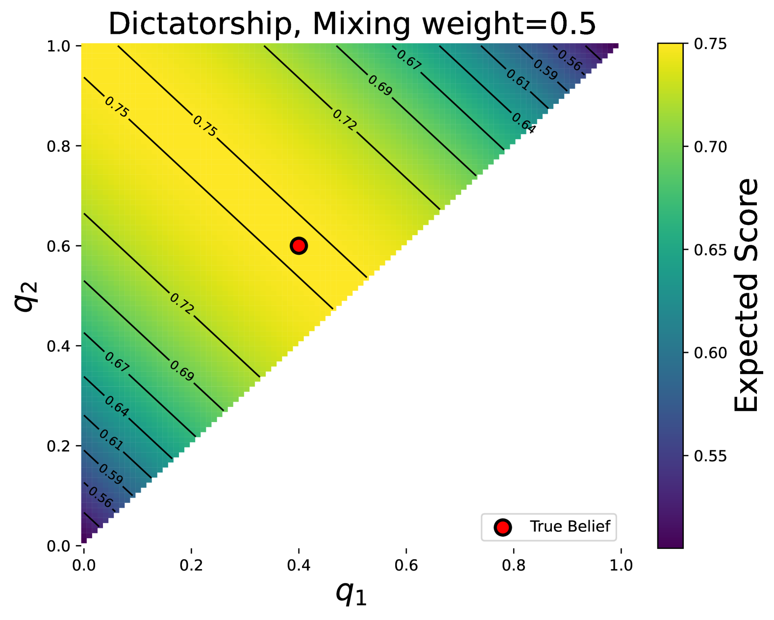
(a)

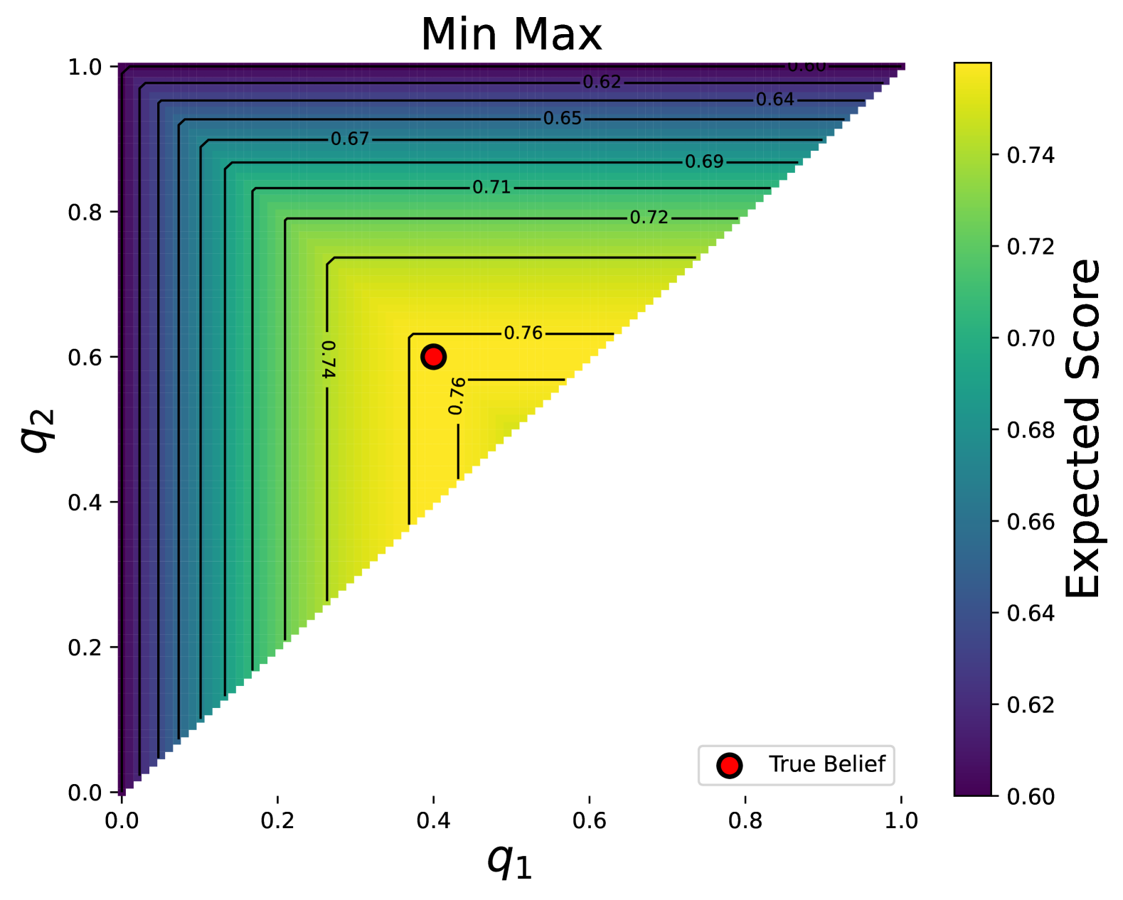
(b)

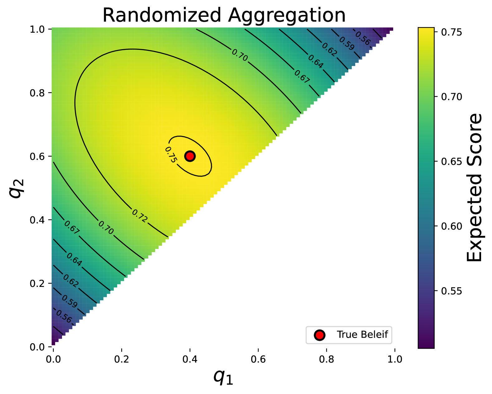
(c)

Figure 3: (Left-to-right) In the first figure we simulate the scoring rule where $\rho$ is a dictatorship with a fixed mixing weight of 0.5, in the middle figure we simulate the scoring rule with min-max $\rho$ (pessimistic decision maker) and in the last figure we simulate the scoring rule where the aggregation is a randomized dictatorship and the forecaster obtains a distribution $\theta=\mathcal{U}[0,1]$ over $\rho$. The lower half of the figure is not plotted since that corresponds to region $q_{1}>q_{2}$, i.e. lower probability being greater than upper probability

Figure˜3 highlights that the randomized scoring rule $s_{\theta}$ is strictly proper for imprecise forecasts as it has the highest expected score for the forecaster only when the forecaster reports his true belief. While in other cases of using a deterministic imprecise scoring rule $s_{\rho}$, if DM provides a $\rho$ such that it is a dictatorship, such as in the case of  Figure˜3(a), the scoring rule is proper; however, the forecaster can lie by reporting the dictator. This can be inferred from the contour that the point $[0.5,0.5]$, which corresponds to the precise forecast $0.5$, also has the highest expected score. With $\rho$ being a min-max rule, the scoring rule $s_{\rho}$ is proper but not strictly as other imprecise forecasts allow the forecaster to obtain the same expected score. For our implementation we consider ${\mathcal{A}}=[0,1]$ and $u(a,o):=(o-a)^{2}$ to satisfy  Lemma˜4.10. We release our implementation at https://github.com/muandet-lab/Imprecise-Scoring-Rule.

References

- Arrow, (1950) Arrow, K. J. (1950). A difficulty in the concept of social welfare. Journal of political economy, 58(4), 328–346.
- Arrow, (2012) Arrow, K. J. (2012). Social choice and individual values, volume 12. Yale university press.
- Augustin et al., (2014) Augustin, T., Coolen, F. P. A., de Cooman, G., & Troffaes, M. C. M. (2014). Introduction to Imprecise Probabilities. Chichester: John Wiley & Sons.
- Bishop & Leeuw, (1959) Bishop, E. & Leeuw, K. D. (1959). The representations of linear functionals by measures on sets of extreme points. In Annales de l’institut Fourier, volume 9 (pp. 305–331).
- Brier, (1950) Brier, G. W. (1950). Verification of forecasts expressed in terms of probability. Monthly Weather Review, 78(1), 1–3.
- Brown, (1981) Brown, L. D. (1981). A complete class theorem for statistical problems with finite sample spaces. The Annals of Statistics, (pp. 1289–1300).
- Caprio, (2024) Caprio, M. (2024). Optimal transport for -contaminated credal sets. arXiv preprint arXiv:2410.03267.
- Caprio et al., (2024) Caprio, M., Sultana, M., Elia, E., & Cuzzolin, F. (2024). Credal Learning Theory. arXiv:2402.00957 [cs, stat].
- Chau et al., (2024) Chau, S. L., Schrab, A., Gretton, A., Sejdinovic, D., & Muandet, K. (2024). Credal two-sample tests of epistemic ignorance. arXiv preprint arXiv:2410.12921.
- Dawid, (1982) Dawid, A. P. (1982). The well-calibrated bayesian. Journal of the American Statistical Association, 77(379), 605–610.
- Dawid, (2007) Dawid, A. P. (2007). The geometry of proper scoring rules. Annals of the Institute of Statistical Mathematics, 59, 77–93.
- de Finetti, (1974) de Finetti, B. (1974). Theory of Probability. John Wiley & Sons.
- Dhillon & Mertens, (1999) Dhillon, A. & Mertens, J.-F. (1999). Relative utilitarianism. Econometrica, 67(3), 471–498.
- Fröhlich & Williamson, (2024) Fröhlich, C. & Williamson, R. C. (2024). Scoring rules and calibration for imprecise probabilities. arXiv preprint arXiv:2410.23001.
- Frongillo & Kash, (2014) Frongillo, R. & Kash, I. (2014). General truthfulness characterizations via convex analysis. In Web and Internet Economics: 10th International Conference, WINE 2014, Beijing, China, December 14-17, 2014. Proceedings 10 (pp. 354–370).: Springer.
- Gajdos et al., (2004) Gajdos, T., Tallon, J.-M., & Vergnaud, J.-C. (2004). Decision making with imprecise probabilistic information. Journal of Mathematical Economics, 40(6), 647–681.
- Gneiting & Katzfuss, (2014) Gneiting, T. & Katzfuss, M. (2014). Probabilistic Forecasting. Annual Review of Statistics and Its Application, 1(1), 125–151. _eprint: https://doi.org/10.1146/annurev-statistics-062713-085831.
- Gneiting & Raftery, (2007) Gneiting, T. & Raftery, A. E. (2007). Strictly proper scoring rules, prediction, and estimation. Journal of the American statistical Association, 102(477), 359–378.
- Gopalan et al., (2021) Gopalan, P., Kalai, A. T., Reingold, O., Sharan, V., & Wieder, U. (2021). Omnipredictors. arXiv preprint arXiv:2109.05389.
- Harsanyi, (1955) Harsanyi, J. C. (1955). Cardinal welfare, individualistic ethics, and interpersonal comparisons of utility. Journal of political economy, 63(4), 309–321.
- Huntley et al., (2014) Huntley, N., Hable, R., & Troffaes, M. C. (2014). Decision making. Introduction to imprecise probabilities, (pp. 190–206).
- Hüllermeier & Waegeman, (2021) Hüllermeier, E. & Waegeman, W. (2021). Aleatoric and Epistemic Uncertainty in Machine Learning: An Introduction to Concepts and Methods. Machine Learning, 110(3), 457–506. arXiv:1910.09457 [cs, stat].
- Johnstone et al., (2011) Johnstone, D. J., Jose, V. R. R., & Winkler, R. L. (2011). Tailored scoring rules for probabilities. Decision Analysis, 8(4), 256–268.
- Konek, (2015) Konek, J. (2015). Epistemic conservativity and imprecise credence. Preprint.
- Konek, (2019) Konek, J. (2019). Ip scoring rules: Foundations and applications. In Proceedings of the Eleventh International Symposium on Imprecise Probabilities: Theories and Applications (pp. 256–264).: PMLR.
- Konek, (2023) Konek, J. (2023). Evaluating imprecise forecasts. In Proceedings of the International Symposium on Imprecise Probability: Theories and Applications, volume 215 (pp. 270–279).: PMLR.
- Levin & Peres, (2017) Levin, D. A. & Peres, Y. (2017). Markov chains and mixing times, volume 107. American Mathematical Soc.
- Mayo-Wilson & Wheeler, (2015) Mayo-Wilson, C. & Wheeler, G. (2015). Accuracy and imprecision: A mildly immodest proposal. Philosophy and Phenomenological Research.
- McCarthy, (1956) McCarthy, J. (1956). Measures of the value of information. Proceedings of the National Academy of Sciences, 42(9), 654–655.
- Muandet et al., (2013) Muandet, K., Balduzzi, D., & Schölkopf, B. (2013). Domain Generalization via Invariant Feature Representation. arXiv:1301.2115 [cs, stat].
- Murphy & Winkler, (1988) Murphy, A. H. & Winkler, R. L. (1988). A new vector partition of the probability score. Journal of Applied Meteorology, 27, 1200–1207.
- Myerson, (1981) Myerson, R. B. (1981). Optimal auction design. Mathematics of Operations Research, 6(1), 58–73.
- Pinson, (2013) Pinson, P. (2013). Wind energy: Forecasting challenges for its operational management.
- Pinson & Girard, (2012) Pinson, P. & Girard, R. (2012). Evaluating the quality of scenarios of short-term wind power generation. Applied Energy, 96, 12–20.
- Richmond et al., (2008) Richmond, J. V., Nau, R. F., & Winkler, R. L. (2008). Scoring rules, generalized entropy, and utility maximization. Operations research, (5), 1146–1157.
- Rindt et al., (2022) Rindt, D., Hu, R., Steinsaltz, D., & Sejdinovic, D. (2022). Survival regression with proper scoring rules and monotonic neural networks. In International Conference on Artificial Intelligence and Statistics (pp. 1190–1205).: PMLR.
- Rudin, (1976) Rudin, W. (1976). Principles of Mathematical Analysis. International Series in Pure and Applied Mathematics. New York: McGraw-Hill, 3rd edition.
- Sale et al., (2023) Sale, Y., Caprio, M., & Hüllermeier, E. (2023). Is the Volume of a Credal Set a Good Measure for Epistemic Uncertainty? arXiv:2306.09586 [cs, stat].
- Savage, (1971) Savage, L. J. (1971). Elicitation of personal probabilities and expectations. Journal of the American Statistical Association, 66(336), 783–801.
- Savage, (1972) Savage, L. J. (1972). The foundations of statistics. Courier Corporation.
- Schoenfield, (2017) Schoenfield, M. (2017). The accuracy and rationality of imprecise credences. Noûs, 51(4), 667–685.
- Seidenfeld et al., (2012) Seidenfeld, T. et al. (2012). Elicitation of imprecise beliefs. In Advances in Imprecise Probability (pp. 89–103). Springer.
- Shao et al., (2024) Shao, C., Meng, F., Liu, Y., & Zhou, J. (2024). Language generation with strictly proper scoring rules. arXiv preprint arXiv:2405.18906.
- Singh et al., (2024) Singh, A., Chau, S. L., Bouabid, S., & Muandet, K. (2024). Domain generalisation via imprecise learning. arXiv preprint arXiv:2404.04669.
- Troffaes, (2007) Troffaes, M. C. (2007). Decision making under uncertainty using imprecise probabilities. International journal of approximate reasoning, 45(1), 17–29.
- Troffaes & de Cooman, (2014) Troffaes, M. C. M. & de Cooman, G. (2014). Lower previsions. In Introduction to Imprecise Probabilities (pp. 159–181). Chichester: John Wiley & Sons.
- Von Neumann & Morgenstern, (1947) Von Neumann, J. & Morgenstern, O. (1947). Theory of games and economic behavior. Princeton university press.
- Walley, (1991) Walley, P. (1991). Statistical Reasoning with Imprecise Probabilities. London: Chapman and Hall.
- Wang et al., (2021) Wang, J., Lan, C., Liu, C., Ouyang, Y., & Qin, T. (2021). Generalizing to unseen domains: A survey on domain generalization. CoRR, abs/2103.03097.
- Wang et al., (2024) Wang, K., Cuzzolin, F., Shariatmadar, K., Moens, D., & Hallez, H. (2024). Credal wrapper of model averaging for uncertainty estimation on out-of-distribution detection. arXiv preprint arXiv:2405.15047.
- Wilks, (2011) Wilks, D. S. (2011). Statistical Methods in the Atmospheric Sciences. Academic Press, 3rd edition.
- Winkler, (1967) Winkler, R. L. (1967). The quantification of judgment: Some methodological suggestions. Journal of the American Statistical Association, 62(320), 1105–1120.
- Wu & Hartline, (2024) Wu, Y. & Hartline, J. (2024). Elicitationgpt: Text elicitation mechanisms via language models. arXiv preprint arXiv:2406.09363.
- Yanagisawa, (2023) Yanagisawa, H. (2023). Proper scoring rules for survival analysis. In International Conference on Machine Learning (pp. 39165–39182).: PMLR.
- Zhou et al., (2023) Zhou, K., Liu, Z., Qiao, Y., Xiang, T., & Loy, C. C. (2023). Domain generalization: A survey. IEEE Transactions on Pattern Analysis and Machine Intelligence, 45(4), 4396–4415.