Intrinsic superconducting diode effect and nonreciprocal superconductivity in rhombohedral graphene multilayers

Abstract

Rhombohedral tetralayer graphene has recently emerged as an exciting platform for a possible chiral superconducting state. Here, we theoretically demonstrate and study the emergence of nonreciprocal superconductivity and an intrinsic superconducting diode effect in this system. Our results are based on a fully self-consistent framework for determining the superconducting order parameter from a Kohn-Luttinger mechanism to superconductivity and show that large diode efficiencies, $\sim 60$%, are achievable and highly tunable by an external displacement field. Moreover, we also find that the diodicity shows a characteristic angular dependence with multiple enhanced lobes, which depend on the Fermi surface structure of the underlying normal state. Hence, our results suggest that the intrinsic superconducting diode effect could provide insights into the type of Fermi surface topology from which superconductivity arises.

Non-reciprocal phenomena in superconducting systems that break time-reversal and inversion symmetry have recently attracted a great deal of attention [1]. A prominent example is the superconducting diode effect (SDE), characterized by a critical current that depends on the current-bias direction [2, 3, 4, 5, 6, 7, 8]. One established route to achieving such a SDE relies on applying an external magnetic field [9, 10, 11, 12, 13, 14, 15, 16, 17, 18] or flux [19, 20, 21, 22, 23, 24, 25, 26] to break time-reversal symmetry. However, it is also possible for certain materials to break the relevant symmetries at the microscopic level, giving rise to an intrinsic SDE [27, 28, 29, 30, 31, 32, 33]. Such an intrinsic SDE could enable field-free non-reciprocal circuit elements [34, 35, 36, 37, 38, 39] and serve as a novel probe for symmetry-breaking in superconducting materials.

In an exciting recent development, superconductivity has been discovered in rhombohedral tetralayer graphene (RTLG) [40, 41]. A unique aspect of RTLG is that a superconducting phase can emerge from a spin- and valley-polarized “quarter-metal” parent state and persists under large in-plane magnetic fields [40]. These observations point to a possible spin-polarized pairing with a chiral $p+ip$ superconducting order parameter, as suggested by theoretical works  [42, 43, 44, 45, 46, 47, 48, 49, 50]. Notably, both time-reversal symmetry (due to the quarter-metal normal state and chiral superconductivity) and inversion symmetry (due to an applied displacement field and trigonal warping) can be broken in RTLG. These symmetry-breaking properties make RTLG a promising platform for non-reciprocal superconducting phenomena. Indeed, an observation of an intrinsic SDE in RTLG has recently been reported [40].

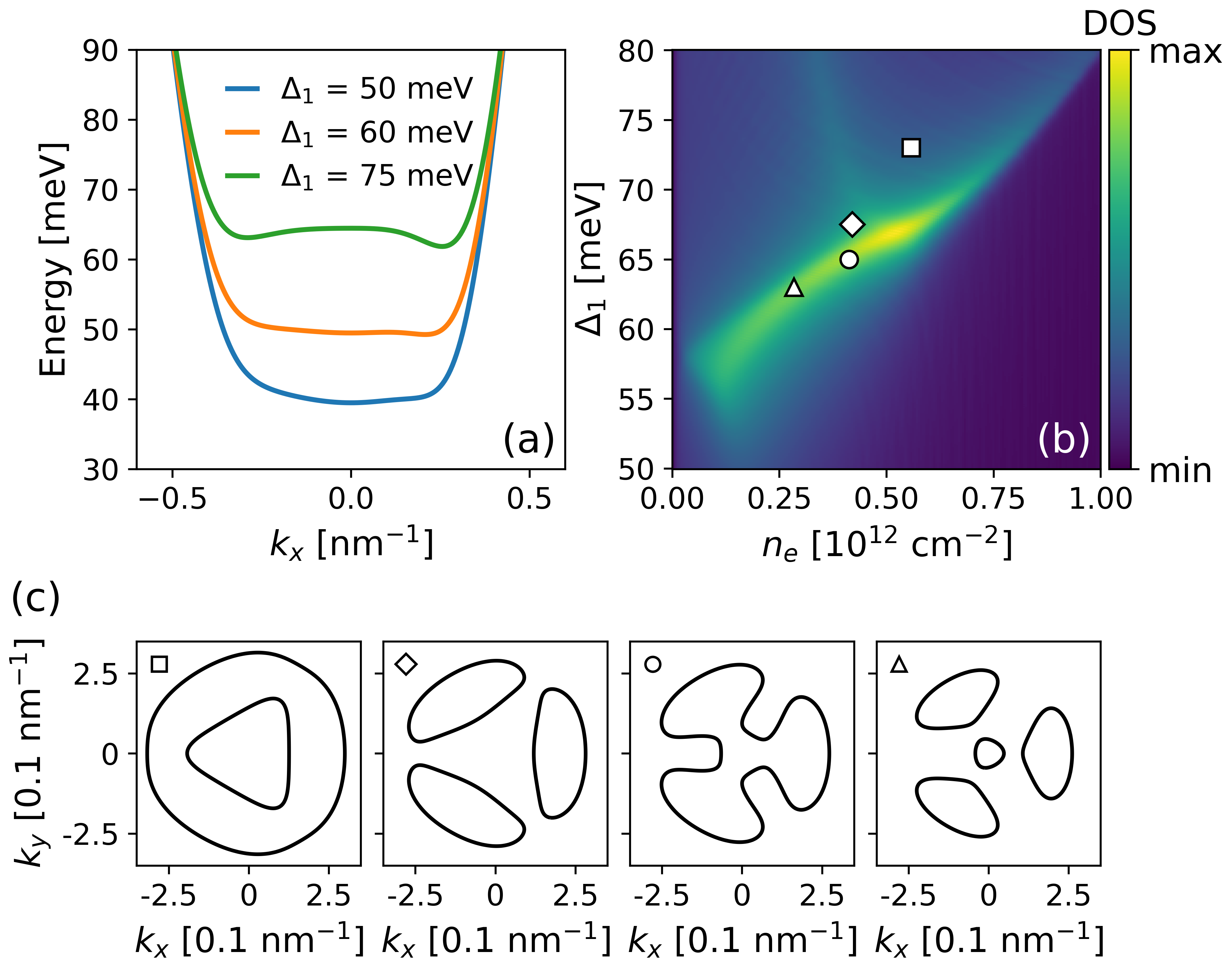
Figure 1: (a) Dispersion of RTLG along the $k_{x}$-direction for different displacement fields, $\Delta_{1}$, showing a band flattening around $k_{x}=0$. (b) Density of states (DOS) of RTLG as a function of $\Delta_{1}$ and the carrier density, $n_{e}$ (relative to the charge neutrality point), showing a significant enhancement due to the band flattening. (c) Fermi surfaces for ($\Delta_{1},n_{e}$), from left to right, set to $(72\,\text{meV},0.574)$, $(67.5\,\text{meV},0.386)$, $(65\,\text{meV},0.414)$, $(63\,\text{meV},0.254)$.

Here, we theoretically demonstrate and study the emergence of nonreciprocal superconductivity, characterized by an asymmetric quasiparticle dispersion, and an intrinsic SDE in RTLG. Our results are based on a fully self-consistent framework for determining the superconducting order parameter from a Kohn-Luttinger mechanism to superconductivity and show that large diode efficiencies, $\sim 60$%, are achievable and highly tunable by an external displacement field. Moreover, we also find that the diodicity shows a characteristic angular dependence with multiple enhanced lobes, which depend on the Fermi surface topology of the underlying normal state. Hence, our results suggest that the intrinsic SDE could provide insights into the type of Fermi surface topology from which superconductivity arises.

Model. We consider a minimal model for spin- and valley-polarized RTLG. The non-interacting part of the Hamiltonian, $H_{0}$, for describing the band structure near the $K$ or $K^{\prime}$ valley (labeled by $\tau=\pm$) is written in the basis $(A_{1},B_{1},A_{2},B_{2},A_{3},B_{3},A_{4},B_{4})$, where $A_{\ell}$ and $B_{\ell}$ denote the sublattices of the $\ell^{\text{th}}$ layer. It is given by [51],

$$H_{0}=$$ (1)

$$\begin{pmatrix}D-\delta&v_{0}\pi^{\dagger}&v_{4}\pi^{\dagger}&v_{3}\pi&0&\frac{\gamma_{2}}{2}&0&0\\ v_{0}\pi&D&\gamma_{1}&v_{4}\pi^{\dagger}&0&0&0&0\\ v_{4}\pi&\gamma_{1}&\frac{D}{3}&v_{0}\pi^{\dagger}&v_{4}\pi^{\dagger}&v_{3}\pi&0&\frac{\gamma_{2}}{2}\\ v_{3}\pi^{\dagger}&v_{4}\pi&v_{0}\pi&\frac{D}{3}&\gamma_{1}&v_{4}\pi^{\dagger}&0&0\\ 0&0&v_{4}\pi&\gamma_{1}&-\frac{D}{3}&v_{0}\pi^{\dagger}&v_{4}\pi^{\dagger}&v_{3}\pi\\ \frac{\gamma_{2}}{2}&0&v_{3}\pi^{\dagger}&v_{4}\pi&v_{0}\pi&-\frac{D}{3}&\gamma_{1}&v_{4}\pi^{\dagger}\\ 0&0&0&0&v_{4}\pi&\gamma_{1}&\delta-D&v_{0}\pi^{\dagger}\\ 0&0&\frac{\gamma_{2}}{2}&0&v_{3}\pi^{\dagger}&v_{4}\pi&v_{0}\pi&-D-\delta\end{pmatrix},$$

where $\pi=\tau k_{x}+ik_{y}$ and the momentum $\boldsymbol{k}=(k_{x},k_{y})$ is measured relative to $K$ or $K^{\prime}$ valley. The $k_{x}$-direction correspond to the $\Gamma$-$K$ direction of the full momentum-space Hamiltonian, while the $k_{y}$-direction corresponds to the $\Gamma$-$M$ direction. The parameters $v_{j}=\sqrt{3}a\gamma_{j}/2$ are given in terms of the graphene lattice constant, $a=2.46$\mathrm{\SIUnitSymbolAngstrom}$$, and the hoppings, $\gamma_{j}$. Moreover, $\delta$ is a sublattice potential and $D$ is an external displacement field. For our simulations, we use $(\gamma_{0},\gamma_{1},\gamma_{2},\gamma_{3},\gamma_{4},\delta)=(3.1,0.38,-0.015,-0.29,-0.141,-0.0105)\,\text{eV}$ [52].

Diagonalizing $H_{0}$ in Eq. (1) shows that the low-energy conduction and valence bands in RTLG originate primarily from the weakly-coupled $A_{1}$ and $B_{4}$ sublattices. These sublattices of the top and bottom layers are only weakly coupled by interlayer hopping, resulting in low-energy bands that touch near the $K$ or $K^{\prime}$ valley. The application of a displacement field, $\Delta_{1}$, opens an energy gap and flattens these lowest bands, leading to a significant enhancement of the density of states, see Fig. 1(a) and (b). Furthermore, a finite $\Delta_{1}$ reverses the band curvature near $\boldsymbol{k}=0$. As a result, the Fermi surface can display multiple connected components depending on $\Delta_{1}$ and the electron density $n_{e}$, see Fig. 1(c).

The aforementioned flattening of the low-energy bands in RTLG enhances the importance of interaction effects. In the recent observation of superconductivity from a spin- and valley-polarized “quarter-metal”, the chemical potential was tuned to the bottom of the lowest conduction band [40]. This motivates us to introduce the following effective Hamiltonian for the interacting system,

$$\begin{split}H_{\text{eff}}&=\sum_{\boldsymbol{k}}\varepsilon_{\boldsymbol{k}}\,c^{\dagger}_{\boldsymbol{k}}c_{\boldsymbol{k}}\\ &+\frac{1}{2\Omega}\sum_{\boldsymbol{k},\boldsymbol{k}^{\prime},\boldsymbol{q}}\tilde{V}_{\boldsymbol{q}}\,F_{\boldsymbol{k},\boldsymbol{k}+\boldsymbol{q}}\,F_{\boldsymbol{k}^{\prime},\boldsymbol{k}^{\prime}-\boldsymbol{q}}\;c_{\boldsymbol{k}}^{\dagger}c_{\boldsymbol{k}+\boldsymbol{q}}c_{\boldsymbol{k}^{\prime}}^{\dagger}c_{\boldsymbol{k}^{\prime}-\boldsymbol{q}}\end{split}$$ (2)

The first term describes the dispersion, $\varepsilon_{\boldsymbol{k}}$, of the lowest conduction band obtained from $H_{0}$ with $c_{\boldsymbol{k}}$ denoting the electron annihilation operator of that band.

Figure 2: (a) Magnitude of the superconducting order parameter, $\Delta_{\boldsymbol{k},\boldsymbol{q}}$, for the Fermi surface shown as an inset in the zero-temperature limit. (b) Phase of the superconducting order parameter, showing a $p+ip$ winding. (c) Quasiparticle dispersion, $E_{\boldsymbol{k,\boldsymbol{q}}}$, associated with the superconducting order parameter shown in (a) and (b). (d) The quasiparticle dispersion is asymmetric under $k_{x}\rightarrow-k_{x}$. Hence, RTLG realizes a nonreciprocal superconductor.

The second term captures interaction effects by projecting a repulsive Coulomb interaction onto the lowest conduction band and accounting for screening effects at the level of the random phase approximation (RPA). This projection introduces the structure factors, $F_{\boldsymbol{k},\boldsymbol{k}+\boldsymbol{q}}=\langle\psi_{\boldsymbol{k}}|\psi_{\boldsymbol{k}+\boldsymbol{q}}\rangle$, that describe the overlap of Bloch states in the lowest conduction band. Moreover, the RPA-screened Coulomb potential is,

$$\tilde{V}_{\boldsymbol{q}}=\frac{V_{\boldsymbol{q}}}{1-\Pi_{\mathbf{q}}V_{\boldsymbol{q}}}.$$ (3)

where $V_{\boldsymbol{q}}=\frac{e^{2}}{2\epsilon}\frac{\tanh(|\boldsymbol{q}|d)}{|\boldsymbol{q}|}$ denotes the gate-screened Coulomb potential with $d$ being the distance to the metallic gates and $\epsilon$ the dielectric permittivity of the hexagonal boron nitride encapsulation. We take $d=20\,\text{nm}$ and $\epsilon=6\epsilon_{0}$ with $\epsilon_{0}$ the vacuum permittivity. The polarization function, $\Pi_{\boldsymbol{q}}$, entering Eq. (3) is given by, $\Pi_{\boldsymbol{q}}=\frac{1}{\Omega}\sum_{\boldsymbol{k}}\frac{n_{F}(\varepsilon_{\boldsymbol{k}+\boldsymbol{q}})-n_{F}(\varepsilon_{\boldsymbol{k}})}{\varepsilon_{\boldsymbol{k}+\boldsymbol{q}}-\varepsilon_{\boldsymbol{k}}}|F_{\boldsymbol{k},\boldsymbol{k}+\boldsymbol{q}}|^{2}$, where $n_{F}$ is the Fermi-Dirac distribution and $\Omega$ the area of the system.

We will now use this effective Hamiltonian to explain the emergence of nonreciprocal superconductivity and an intrinsic SDE in RTLG.

Nonreciprocal superconductivity. We begin by discussing the emergence of nonreciprocal superconductivity. Nonreciprocal superconductors are a recently proposed class of superconductors in which the breaking of time-reversal and inversion symmetry leads to an asymmetric quasiparticle dispersion [53]. A possible mechanism for such nonreciprocity is finite-momentum pairing. However, as noted in previous works, the Cooper-pair momentum $\boldsymbol{q}$ (defined relative to the $K$ or $K^{\prime}$ valley) in RTLG can be small [44, 45]. We will now explicitly show that the primary origin of the asymmetric quasiparticle dispersion in RTLG is the intrinsic asymmetry of the normal-state band structure, $\varepsilon_{\boldsymbol{k}}\neq\varepsilon_{-\boldsymbol{k}}$. Nevertheless, a finite Cooper-pair momentum can still qualitatively modify the symmetry properties of the quasiparticle dispersion.

To describe the superconductivity in RTLG, we consider, inspired by earlier works [42, 43, 44, 45, 46, 47], a Kohn-Luttinger mechanisms [54, 55, 51, 56, 57]. Specifically, while the bare Coulomb potential, $V_{\boldsymbol{q}}$, is nominally repulsive, the screening effects described by Eq. (3) can lead to an “overscreening” regime, where the effective interaction becomes attractive. This effective attraction can be verified by transforming $\tilde{V}_{\mathbf{q}}$ to real space.

We will assume that this effective attraction can lead to pairing between momentum states $\boldsymbol{k}+\frac{\boldsymbol{q}}{2}$ and $-\boldsymbol{k}+\frac{\boldsymbol{q}}{2}$ where $\boldsymbol{q}$ is the Cooper-pair momentum. While we retain the possibility of a finite $\boldsymbol{q}$, we emphasize that it is not a necessary ingredient for the nonreciprocal superconductivity and SDE. We then perform a mean-field decoupling of the interaction in Eq. (2) in the Cooper channel. The superconducting order parameter is determined self-consistently as,

$$\begin{split}\Delta_{\boldsymbol{k},\boldsymbol{q}}=&-\sum_{\boldsymbol{k}^{\prime}}g_{\boldsymbol{k},\boldsymbol{k}^{\prime},\boldsymbol{q}}\,\frac{\Delta_{\boldsymbol{k}^{\prime},\boldsymbol{q}}}{2\tilde{E}_{\boldsymbol{k}^{\prime},\boldsymbol{q}}}\\ \times&\frac{1}{2}\left\{\tanh\left(\frac{\beta E_{\boldsymbol{k}^{\prime},\boldsymbol{q}}}{2}\right)+\tanh\left(\frac{\beta E_{-\boldsymbol{k}^{\prime},\boldsymbol{q}}}{2}\right)\right\}.\end{split}$$ (4)

where $g_{\boldsymbol{k},\boldsymbol{k}^{\prime},\boldsymbol{q}}=\tilde{V}_{\boldsymbol{k}^{\prime}-\boldsymbol{k}}F_{\boldsymbol{k}+\frac{\boldsymbol{q}}{2},\boldsymbol{k}^{\prime}+\frac{\boldsymbol{q}}{2}}F_{-\boldsymbol{k}+\frac{\boldsymbol{q}}{2},-\boldsymbol{k}^{\prime}+\frac{\boldsymbol{q}}{2}}$ is the pairing interaction, $1/\beta=k_{B}T$, and the quasiparticle dispersion is given by,

$$E_{\boldsymbol{k},\boldsymbol{q}}=\xi_{\boldsymbol{k},\boldsymbol{q},-}+\sqrt{(\xi_{\boldsymbol{k},\boldsymbol{q},+})^{2}+|\Delta_{\boldsymbol{k},\boldsymbol{q}}|^{2}}$$ (5)

Here, we have defined the symmetric and antisymmetric components of the normal-state dispersion as $\xi_{\boldsymbol{k},\boldsymbol{q},\pm}=(\varepsilon_{\boldsymbol{k}+\frac{\boldsymbol{q}}{2}}\pm\varepsilon_{-\boldsymbol{k}+\frac{\boldsymbol{q}}{2}})/2$. Moreover, we have introduced the reduced quasiparticle dispersion, $\tilde{E}_{\boldsymbol{k}^{\prime},\boldsymbol{Q}}=E_{\boldsymbol{k},\boldsymbol{q}}-\xi_{\boldsymbol{k},\boldsymbol{q},-}$.

Next, we solve for $\Delta_{\boldsymbol{k},\boldsymbol{q}}$ self-consistently, imposing a fixed electron density $n_{e}=\sum_{\boldsymbol{k}}\langle c^{\dagger}_{\boldsymbol{k}}c_{\boldsymbol{k}}\rangle/\Omega$ and varying $\boldsymbol{q}$. The realized superconducting order, $\Delta_{\boldsymbol{k},\boldsymbol{q}}$, is determined by minimizing the free energy,

$$F =-\sum_{\boldsymbol{k}}\left\{\frac{1}{\beta}\ln(1+e^{-\beta E_{\boldsymbol{k},\boldsymbol{q}}})-\frac{1}{2}(\xi_{\boldsymbol{k},\boldsymbol{q},+}-\tilde{E}_{\boldsymbol{k},\boldsymbol{q}})\right.$$ (6)

$$\qquad-\left.\frac{\absolutevalue{\Delta_{\boldsymbol{k},\boldsymbol{q}}}^{2}}{8\tilde{E}_{\boldsymbol{k},\boldsymbol{q}}}\left[\tanh\left(\frac{\beta E_{\boldsymbol{k},\boldsymbol{q}}}{2}\right)+\tanh\left(\frac{\beta E_{-\boldsymbol{k},\boldsymbol{q}}}{2}\right)\right]\right\}$$

An example result of self-consistency calculation is shown in Fig. 2(a) and (b) for a Fermi surface with an annulus topology. We see that the superconducting order parameter exhibits a $p+ip$ phase winding. The Cooper-pair momentum is found to be small but finite (${q}_{0}=-$0.004\text{\,}\mathrm{n}\mathrm{m}^{-1}$$), oriented along the $q_{x}$-direction (i.e., the $\Gamma$-$K$ direction). Using the self-consistent solution, we then compute the quasiparticle dispersion, $E_{\boldsymbol{k},\boldsymbol{q}}$, see Fig. 2(c). The quasiparticle dispersion is in general found to be asymmetric with respect to $\boldsymbol{k}\rightarrow-\boldsymbol{k}$. Hence, RTLG realizes nonreciprocal superconductivity. Writing $\boldsymbol{k}=(k\cos\theta,k\sin\theta)$, we see that the asymmetry is most pronounced along $\theta\in\{0^{\circ},60^{\circ},120^{\circ}\}$. It is instructive to discuss these results from a symmetry perspective.

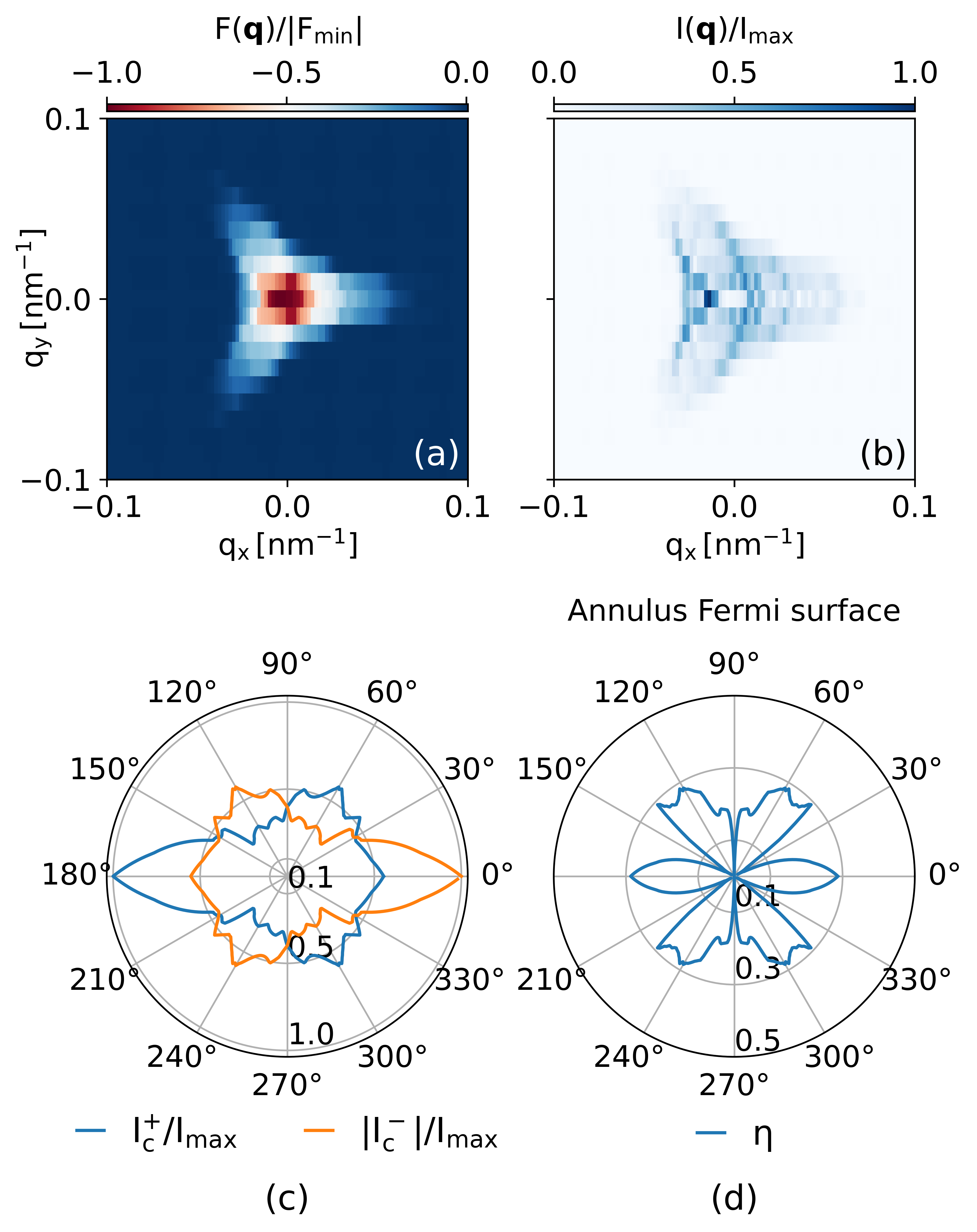
Figure 3: (a) Free energy, $F$, versus $\boldsymbol{q}=(q_{x},q_{y})$ for the annulus Fermi surface shown in Fig. 2. Here, $F_{\text{min}}\equiv\text{min}_{\boldsymbol{q}}\{F(\boldsymbol{q})\}.$ (b) Corresponding supercurrent magnitude, $I$, as a function of $\boldsymbol{q}$. Here, $I_{\text{max}}\equiv\text{max}_{\boldsymbol{q}}\{I(\boldsymbol{q})\}$. (c) Critical currents in the forward direction ($I_{c,+}$) and reverse direction ($I_{c,-}$) for current direction given by an angle $\theta$ relative to the $x$-direction. (d) Diode efficiency for a current direction given by an angle $\theta$.

First, we assume $\boldsymbol{q}=0$. The normal state spectrum is invariant under two three-fold rotations ($2C_{3}$) and three two-fold rotations ($3C_{2}^{\prime}$) around the in-plane axis pointing along $\theta\in\{0^{\circ},60^{\circ},120^{\circ}\}$. Consider a $\boldsymbol{k}$ pointing along one of the directions $\theta\in\{90^{\circ},150^{\circ},30^{\circ}\}$. Then, $C_{2}^{\prime}\boldsymbol{k}=-\boldsymbol{k}$ and hence $\varepsilon_{-\boldsymbol{k}}=\varepsilon_{C_{2}^{\prime}\boldsymbol{k}}=\varepsilon_{\boldsymbol{k}}$. As a result, $\xi_{\boldsymbol{k},\boldsymbol{q},-}=0$ and $E_{\boldsymbol{k},\boldsymbol{q}}=E_{-\boldsymbol{k},\boldsymbol{Q}}$ (since $|\Delta_{\boldsymbol{k},\boldsymbol{q}}|=|\Delta_{-\boldsymbol{k},\boldsymbol{q}}|$). Consequently, if $\boldsymbol{q}=0$, the quasiparticle spectrum is symmetric along the directions $\theta\in\{90^{\circ},150^{\circ},30^{\circ}\}$, but asymmetric otherwise.

Now assume $\boldsymbol{q}\neq 0$. In this case, a vanishing asymmetry of the quasiparticle spectrum requires both $C_{2}^{\prime}\boldsymbol{k}=-\boldsymbol{k}$ and $C_{2}^{\prime}\boldsymbol{q}=\boldsymbol{q}$. In our simulations, we found that $\boldsymbol{q}$ typically pointed along the $\theta=0^{\circ}$ directions so that the two conditions can only be satisfied for momenta $\boldsymbol{k}$ with $\theta=90^{\circ}$. Consequently, the quasiparticle dispersion can be strictly symmetric only along $\theta=90^{\circ}$; in all other directions, it remains asymmetric.

One experimental manifestation of the asymmetric quasiparticle dispersion is that a transparent normal-metal–superconductor junction can exhibit a current-voltage ($I$-$V$) characteristic that is not invariant under $V\rightarrow-V$ [53]. Our results suggest the following probe of the nonreciprocal superconductivity in RTLG: connect two normal leads to the RTLG superconductor, one along $\theta=0^{\circ}$ ($\Gamma$-$K$ direction) and one along $\theta=90^{\circ}$ ($\Gamma$-$M$ direction). Our results imply that the lead along $\theta=0^{\circ}$ would show an asymmytric $I$-$V$ curve, while the $I$-$V$ curve along $\theta=90^{\circ}$ would remain symmetric.

Intrinsic SDE. We are now in the position to evaluate the SDE for RTLG. For this purpose, we self-consistently solve for the superconducting order parameter for a broader range of Cooper-pair momenta, $\boldsymbol{q}$, and use the obtained $\Delta_{\boldsymbol{k},\boldsymbol{q}}$ to evaluate the free energy. The results of the free energy are shown in Fig. 3(a). The current in the ground state that minimizes $F(\mathbf{q})$ is always zero. However, applying a finite current-bias, produces a state with a finite Cooper-pair momentum different from the ground state value, $\boldsymbol{q}\neq\boldsymbol{q}_{0}$. The current in this state is $I=(2e/\hbar)|\partial_{\boldsymbol{q}}F(\boldsymbol{q})|$ [13].

As a next step, we compute the supercurrent versus $\boldsymbol{q}$ are shown in Fig. 3(b). Upon fixing a direction, $\theta$, so that $\boldsymbol{q}=(q\cos\theta,q\sin\theta)$, this allows us to determine the critical current in the forward direction, $I_{c,+}\equiv\text{max}_{q>0}\{I(q,\theta)\}$ and in the reversed direction as, $I_{c,-}\equiv\text{max}_{q>0}\{I(q,\theta+\pi)\}$. The diode efficiency is then defined as,

$$\eta=\frac{|I^{+}_{c}-I^{-}_{c}|}{I^{+}_{c}+I^{-}_{c}}.$$ (7)

Here, we defined $\eta$ as non-negative. However, we remark that the modified efficiency $\eta_{\text{signed}}=\frac{I^{+}_{c}-I^{-}_{c}}{I^{+}_{c}+I^{-}_{c}}$ can exhibit sign changes when transitioning through $\eta=0$ [58].

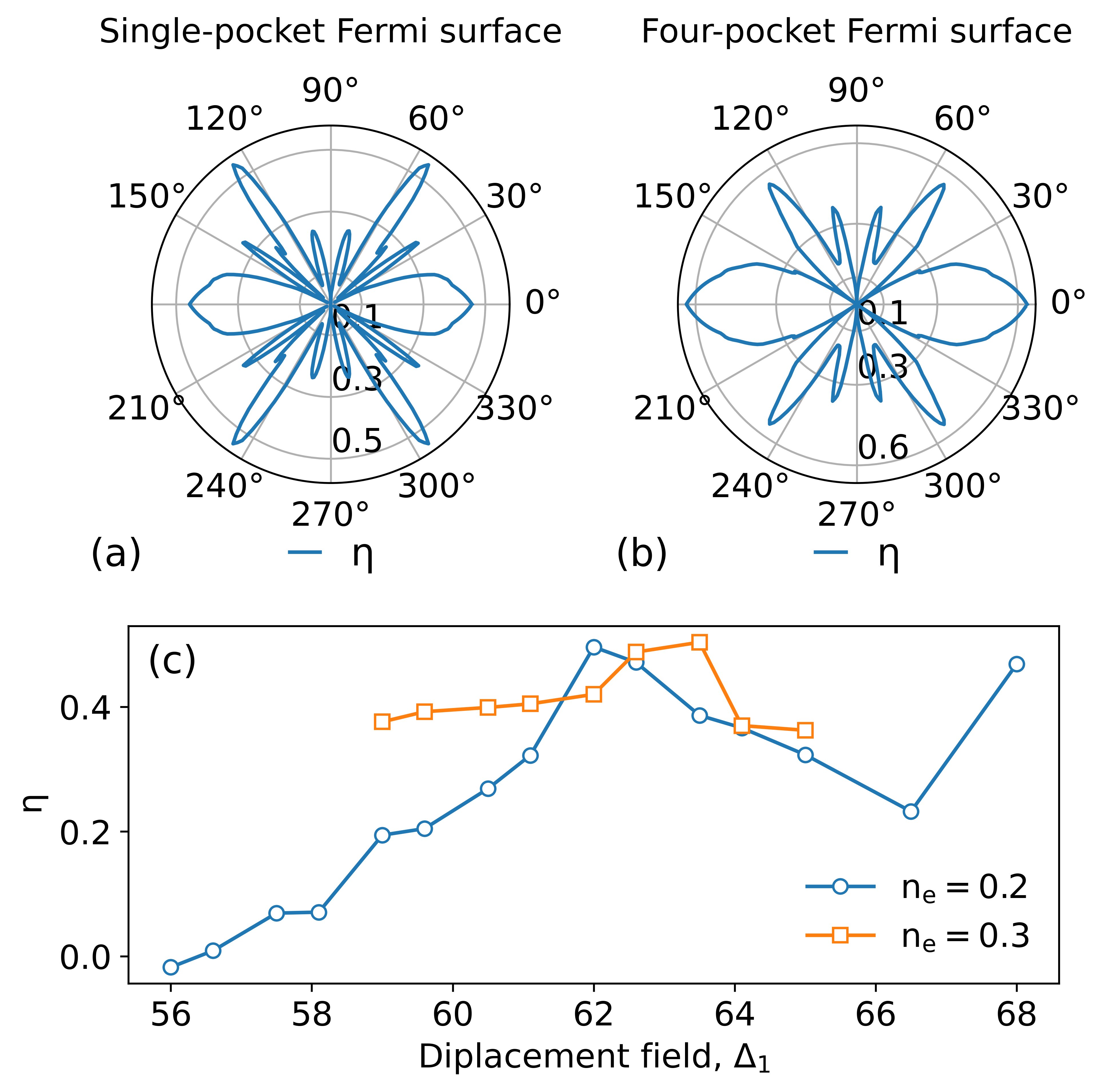
Figure 4: (a) Angular dependence of the diode efficiency, $\eta$, for the single-pocket Fermi surface shown in Fig. 1(c). (b) Same as (a) but for the four-pocket Fermi surface shown in Fig. 1(c). (c) Diode efficiency, $\eta$, versus the displacement field along the $q_{x}$ direction for different electron densities, $n_{e}$.

We begin by evaluating the angular dependence of the critical currents and diode efficiencies for fixed $\Delta_{1}$ and $n_{e}$. Our results are shown in Fig. 3(c) and (d) for a Fermi surface with annulus topology. We find that, in general, the diode efficiency takes on finite values. This verifies the emergence of an intrinsic SDE from a fully self-consistent calculation. Furthermore, we find that $\eta$ exhibits a characteristic multi-lobe structure. Specifically, we see that the efficiency tends to be maximized along the directions $\theta\in\{0^{\circ},60^{\circ},120^{\circ}\}$, reaching values of $\sim 30\%$ for the annulus Fermi surface. In addition, it is strongly suppressed along the directions $\theta\in\{30^{\circ},90^{\circ},150^{\circ}\}$. Moreover, the efficiency in the $\theta=0^{\circ},90^{\circ}$ lobes is functionally different from the remaining lobes. We attribute this difference to the small but finite Cooper-pair momentum along $q_{x}$.

It is now interesting to compare these results for the annulus Fermi surface with other Fermi surface topologies. Our results for a single-pocket Fermi surface and a four-pocket Fermi surface are shown in Fig. 4(a) and (b). We see that the shape of the lobes changes qualitatively. Specifically, the width of the lobes around $\theta\in\{60^{\circ},120^{\circ}\}$ is significantly reduced. Furthermore, in these lobes, the maximum efficiency is achieved slightly away from $\theta=60^{\circ},120^{\circ}$. The overall highest efficiency is found for the four-pocket Fermi surface at $\sim 60\%$. These results suggest that the Fermi surface topology can affect the angular dependence of the diode efficiency and, as a result, could provide insights into the type of Fermi surface topology from which the superconducting state arises. We provide more detailed plots of the free energies and critical currents for single-pocket and four-pocket Fermi surface in the Supplemental Material [58].

Finally, we have also investigated the diode efficiency as a function of the diplacement field, $\Delta_{1}$, for different densities, $n_{e}$, and along the fixed $q_{x}$-direction. Our results are shown in Fig. 4(c). We find that, in general, that the diode efficiency seems to increase with increasing displacement field. However, we remark that the system can enter a metallic phase if the displacement field is increased beyond a density-dependent threshold.

Conclusion. In this work, we have theoretically demonstrated and studied the emergence of an intrinsic SDE and non-reciprocal superconductivity in RTLG through a fully self-consistent approach to determining the superconducting order parameter. Our results suggest that angular dependence of the diodicity in RTLG could provide insights into the type of Fermi surface topology from which superconductivity arises.

Note added. We have recently become aware of a related work [50].

Acknowledgement. We acknowledge helpful discussions with Marco Valentini.

Supplemental Material to ‘Intrinsic superconducting diode effect and nonreciprocal superconductivity in rhombohedral graphene multilayers’

In the Supplemental Material, we provide details on the angular dependence of the diode efficiency and the the mean-field approach for describing the superconducting RTLG system.

1 Angular-dependence of the diode efficiency

In this first section of the Supplementary Material, we provide more details on the angular dependence of the diode efficiency for different Fermi surfaces. We also suggest a possible experimental setup to probe the angular dependence of the diodicity.

Specifically, the obtained angular dependence of the diodicity for a single-pocket Fermi surface and a four-pocket Fermi surface (as shown in Fig. 1(c) in the main text) are given in Fig. 5 and Fig. 6. We also show the signed diode efficiency, $\eta_{signed}$, for the annulus Fermi surface in Fig. 7.

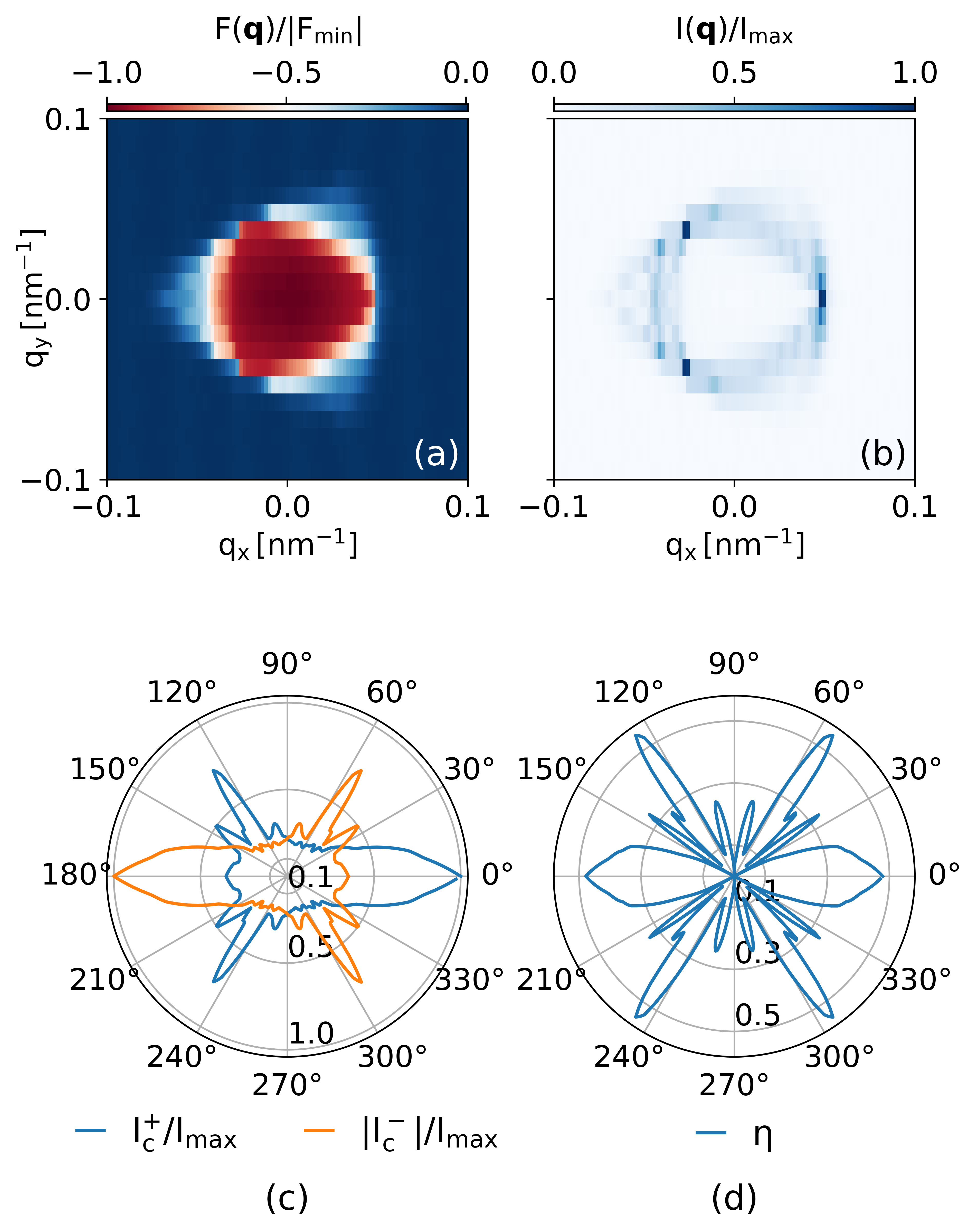
Figure 5: Results for a Fermi surface with one connected components (as shown in Fig. 1(c) of the main text). (a) Free energy, $F$, as a function of $\boldsymbol{q}=(q_{x},q_{y})$. Here, $F_{\text{min}}\equiv\text{min}_{\boldsymbol{q}}F(\boldsymbol{q}).$ (b) Corresponding supercurrent magnitude, $I$, as a function of $\boldsymbol{q}$. Here, $I_{\text{max}}\equiv\text{max}_{\boldsymbol{q}}I(\boldsymbol{q})$. (c) Critical currents in the forward direction ($I_{c,+}$) and reverse direction ($I_{c,-}$) for current direction given by an angle $\theta$ relative to the $x$-direction. (d) Diode efficiency for a current direction given by an angle $\theta$.

To measure the angular dependence of the diode efficiency, we propose a possible experimental setup, which is schematically shown in Fig. 8 and inspired by [29]. In the proposed setup, a circular superconducting RTLG system is connected to multiple leads. Applying a current-bias across the different possible directions would allow for a measurement of the critical currents and the diodicity along the different directions.

Figure 6: Results for a Fermi surface with four connected components (as shown in Fig. 1(c) of the main text). (a) Free energy, $F$, as a function of $\boldsymbol{q}=(q_{x},q_{y})$. Here, $F_{\text{min}}\equiv\text{min}_{\boldsymbol{q}}F(\boldsymbol{q}).$ (b) Corresponding supercurrent magnitude, $I$, as a function of $\boldsymbol{q}$. Here, $I_{\text{max}}\equiv\text{max}_{\boldsymbol{q}}I(\boldsymbol{q})$. (c) Critical currents in the forward direction ($I_{c,+}$) and reverse direction ($I_{c,-}$) for current direction given by an angle $\theta$ relative to the $x$-direction. (d) Diode efficiency for a current direction given by an angle $\theta$.

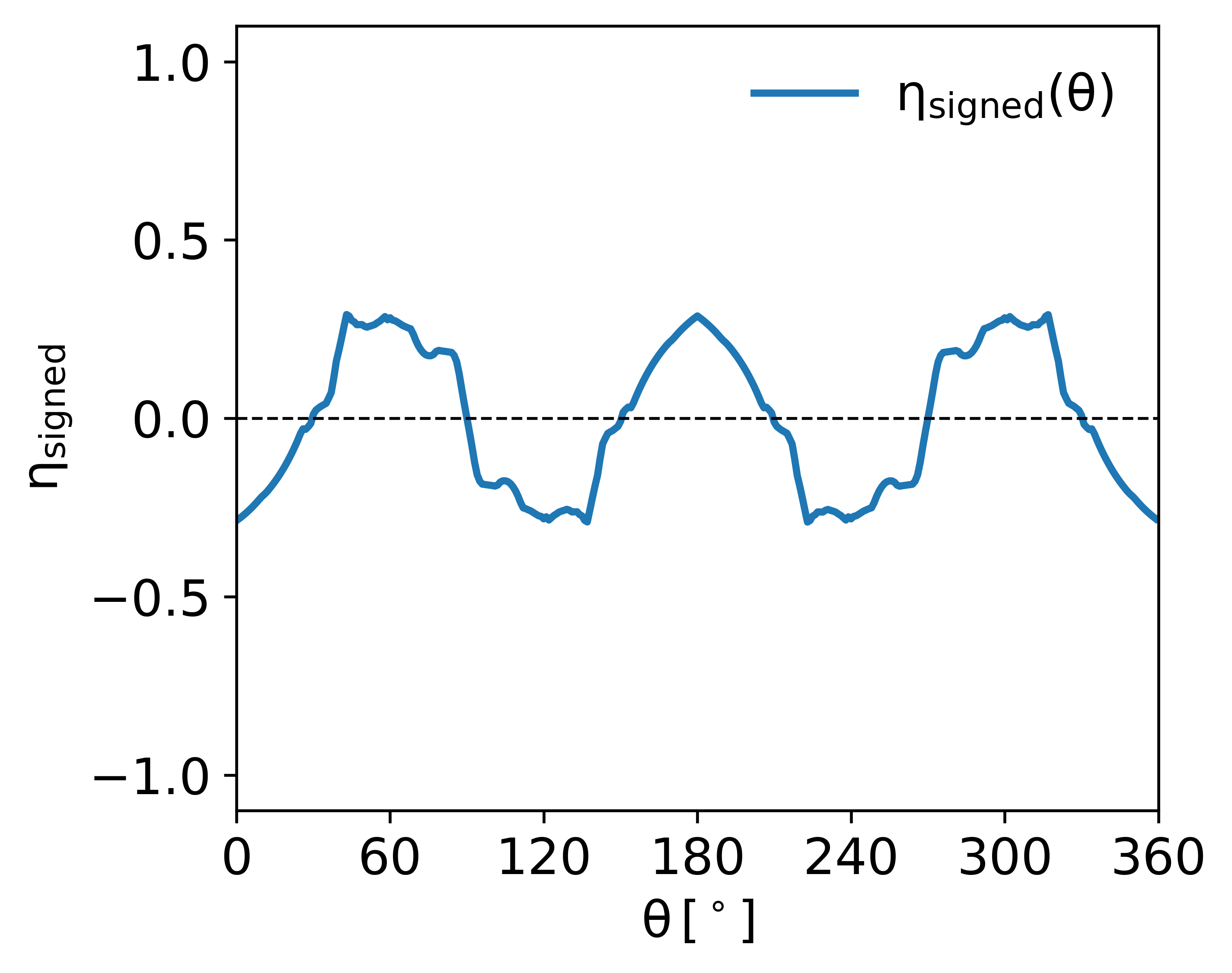
Figure 7: Signed diode efficiency, $\eta_{\text{signed}}$ as a function of the angle, $\theta$, for the annulus fermi surface discussed in Fig. 3 of the main text.

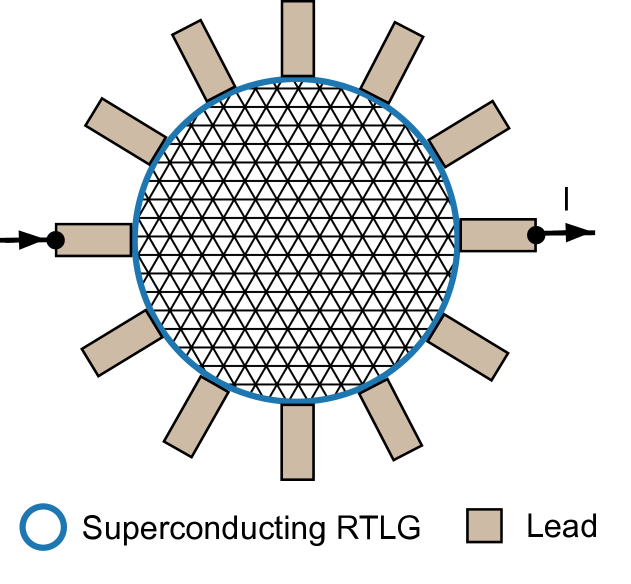
Figure 8: Possible setup for determining the angular dependence of diode efficiency in RTLG, inspired by [29]. A circular superconducting RTLG sample is connected to multiple leads. Application of a current bias, $I$, along the different directions enables the extraction of the critical currents and diode efficiencies.

2 Mean-field decoupling

In this second section of the Supplementary Material, we provide a detailed discussion of the mean-field decoupling of the effective interaction Hamiltonian.

We consider only scattering processes of electron pairs with a finite Cooper-pair momentum, $\boldsymbol{q}$. Then the effective Hamiltonian of the interacting systems can be written as,

$$\begin{split}H_{\text{eff}}&\rightarrow\sum_{\boldsymbol{k}}\varepsilon_{\boldsymbol{k}}\,c^{\dagger}_{\boldsymbol{k}}c_{\boldsymbol{k}}\\ &+\frac{1}{2\Omega}\sum_{\boldsymbol{k},\boldsymbol{k}^{\prime},\boldsymbol{q}}g_{\boldsymbol{k},\boldsymbol{k}^{\prime},\boldsymbol{q}}\,c_{\boldsymbol{k}+\frac{\boldsymbol{Q}}{2}}^{\dagger}c_{-\boldsymbol{k}+\frac{\boldsymbol{Q}}{2}}^{\dagger}c_{-\boldsymbol{k^{\prime}}+\frac{\boldsymbol{Q}}{2}}c_{\boldsymbol{k^{\prime}}+\frac{\boldsymbol{Q}}{2}}\end{split}$$ (8)

with the pairing interaction, $g_{\boldsymbol{k},\boldsymbol{k}^{\prime},\boldsymbol{q}}\,=\tilde{V}_{\boldsymbol{k}^{\prime}-\boldsymbol{k}}F_{\boldsymbol{k}+\frac{\boldsymbol{q}}{2},\boldsymbol{k}^{\prime}+\frac{\boldsymbol{q}}{2}}F_{-\boldsymbol{k}+\frac{\boldsymbol{q}}{2},-\boldsymbol{k}^{\prime}+\frac{\boldsymbol{q}}{2}}$.

Next, we introduce the mean-field,

$$b_{\boldsymbol{k^{\prime}},\boldsymbol{Q}}\equiv\bigl{\langle}c_{-\boldsymbol{k^{\prime}}+\frac{\boldsymbol{q}}{2}}\,c_{\boldsymbol{k^{\prime}}+\frac{\boldsymbol{q}}{2}}\bigr{\rangle},$$ (9)

which produces the following mean-field Hamiltonian,

$$H_{\text{MF}}=\sum_{\boldsymbol{k}}\varepsilon_{\boldsymbol{k}}\,c^{\dagger}_{\boldsymbol{k}}c_{\boldsymbol{k}}-\frac{1}{2}\sum_{\boldsymbol{k}}\left\{\Delta_{\boldsymbol{k},\boldsymbol{q}}^{*}c_{-\boldsymbol{k}+\frac{\boldsymbol{q}}{2}}c_{\boldsymbol{k}+\frac{\boldsymbol{q}}{2}}+\Delta_{\boldsymbol{k},\boldsymbol{q}}c_{\boldsymbol{k}+\frac{\boldsymbol{q}}{2}}^{\dagger}c_{-\boldsymbol{k}+\frac{\boldsymbol{q}}{2}}^{\dagger}\right\}+K_{0,\boldsymbol{q}}$$ (10)

with

$$K_{0,\boldsymbol{q}}=\frac{1}{2}\sum_{\boldsymbol{k}}\Delta_{\boldsymbol{k},\boldsymbol{q}}b_{\boldsymbol{k},\boldsymbol{q}}^{*}.$$ (11)

In the expression for the mean-field Hamiltonian, we have defined the superconducting order parameter as,

$$\Delta_{\boldsymbol{k},\boldsymbol{q}}=-\frac{1}{\Omega}\sum_{\boldsymbol{k^{\prime}}}g_{\boldsymbol{k},\boldsymbol{k^{\prime}},\boldsymbol{q}}b_{\boldsymbol{k^{\prime}},\boldsymbol{q}}.$$ (12)

We note that $g_{\boldsymbol{k},\boldsymbol{k}^{\prime},\boldsymbol{q}}=g_{-\boldsymbol{k},-\boldsymbol{k}^{\prime},\boldsymbol{q}}$ and $b_{\boldsymbol{k},\boldsymbol{Q}}=-b_{-\boldsymbol{k},\boldsymbol{Q}}$ from the fermionic anticommutation relations. Hence, the order parameter needs to satisfy,

$$\Delta_{\boldsymbol{k},\boldsymbol{q}}=-\Delta_{-\boldsymbol{k},\boldsymbol{q}}.$$ (13)

3 Bogoliubov-de Gennes Hamiltonian

In this third section of the Supplemental Material, we provide details on the derivation of the Bogoliubov-de Gennes Hamiltonian for rhombohedral tetralayer graphene and its diagonalization procedure.

3.1 Hamiltonian formulation

As a starting point, we write down the full system Hamiltonian as,

$$H_{\text{MF},\boldsymbol{q}}=H_{0}+H_{\Delta},$$ (14)

where $H_{0}$ represents the normal-state Hamiltonian and $H_{\Delta}$ is the pairing Hamiltonian.

First, for the normal-state Hamiltonian, we write,

$$\begin{split}H_{0}&=\sum_{\boldsymbol{k}}\varepsilon_{\boldsymbol{k}}c_{\boldsymbol{k}}^{\dagger}c_{\boldsymbol{k}}\\ &=\sum_{\boldsymbol{k}\in\text{BZ}_{+}}\varepsilon_{\boldsymbol{k}+\frac{\boldsymbol{q}}{2}}c_{\boldsymbol{k}+\frac{\boldsymbol{q}}{2}}^{\dagger}c_{\boldsymbol{k}+\frac{\boldsymbol{q}}{2}}+\sum_{\boldsymbol{k}\in\text{BZ}_{+}}\varepsilon_{-\boldsymbol{k}+\frac{\boldsymbol{q}}{2}}c_{-\boldsymbol{k}+\frac{\boldsymbol{q}}{2}}c_{-\boldsymbol{k}+\frac{\boldsymbol{q}}{2}}^{\dagger}+K_{1,\boldsymbol{q}},\end{split}$$ (15)

where the dispersion $\varepsilon_{\boldsymbol{k}}$ corresponds to the lowest conduction band. In this expression, the Brillouin zone is partitioned as $\text{BZ}_{+}\equiv\left\{\boldsymbol{k}=(k_{x},k_{y})\in\text{BZ}\,\middle|\,k_{x}>0\right\}$ and $\text{BZ}_{-}\equiv\left\{\boldsymbol{k}=(k_{x},k_{y})\in\text{BZ}\,\middle|\,k_{x}<0\right\}$. Moreover, the energy offset is defined as

$$K_{1,\boldsymbol{q}}\equiv\sum_{\boldsymbol{k}\in\text{BZ}_{+}}\varepsilon_{-\boldsymbol{k}+\frac{\boldsymbol{q}}{2}}.$$ (16)

Second, the pairing Hamiltonian is written as

$$\begin{split}H_{\Delta}&=K_{0,\boldsymbol{q}}-\frac{1}{2}\sum_{\boldsymbol{k}\in\text{BZ}_{+}}\left\{\Delta_{\boldsymbol{k},\boldsymbol{q}}\,c_{\boldsymbol{k}+\frac{\boldsymbol{q}}{2}}^{\dagger}c_{-\boldsymbol{k}+\frac{\boldsymbol{q}}{2}}^{\dagger}+\Delta_{-\boldsymbol{k},\boldsymbol{q}}\,c_{-\boldsymbol{k}+\frac{\boldsymbol{q}}{2}}^{\dagger}c_{\boldsymbol{k}+\frac{\boldsymbol{q}}{2}}^{\dagger}+\text{h.c.}\right\}\\ &=K_{0,\boldsymbol{q}}-\sum_{\boldsymbol{k}\in\text{BZ}_{+}}\left\{\Delta_{\boldsymbol{k},\boldsymbol{q}}\,c_{\boldsymbol{k}+\frac{\boldsymbol{q}}{2}}^{\dagger}c_{-\boldsymbol{k}+\frac{\boldsymbol{q}}{2}}^{\dagger}+\text{h.c.}\right\},\end{split}$$ (17)

Hence, the full Hamiltonian can be written as

$$H=K_{0,\boldsymbol{q}}+K_{1,\boldsymbol{q}}+\sum_{\boldsymbol{k}\in\text{BZ}_{+}}\Psi_{\boldsymbol{k},\boldsymbol{q}}^{\dagger}\mathcal{H}_{\text{BdG},\boldsymbol{k},\boldsymbol{q}}\Psi_{\boldsymbol{k},\boldsymbol{q}},\quad\text{with}\quad\mathcal{H}_{\text{BdG},\boldsymbol{k},\boldsymbol{q}}\equiv\begin{pmatrix}\varepsilon_{\boldsymbol{k}+\frac{\boldsymbol{q}}{2}}&-\Delta_{\boldsymbol{k},\boldsymbol{q}}\\ -\Delta_{\boldsymbol{k},\boldsymbol{q}}^{*}&-\varepsilon_{-\boldsymbol{k}+\frac{\boldsymbol{q}}{2}}\end{pmatrix}$$ (18)

and the Nambu spinor, $\Psi_{\boldsymbol{k},\boldsymbol{q}}\equiv(c_{\boldsymbol{k}+\frac{\boldsymbol{q}}{2}},c_{-\boldsymbol{k}+\frac{\boldsymbol{q}}{2}}^{\dagger})^{T}.$

3.2 Hamiltonian Diagonalization

To diagonalize $\mathcal{H}_{\text{BdG},\boldsymbol{k},\boldsymbol{q}}$, we first introduce the dispersions

$$\xi_{\boldsymbol{k},\boldsymbol{q},\pm}=\frac{\varepsilon_{\boldsymbol{k}+\frac{\boldsymbol{q}}{2}}\pm\varepsilon_{-\boldsymbol{k}+\frac{\boldsymbol{q}}{2}}}{2},$$ (19)

with $\xi_{\boldsymbol{k},\boldsymbol{q},+}=\xi_{-\boldsymbol{k},\boldsymbol{q},+}$ and $\xi_{\boldsymbol{k},\boldsymbol{q},-}=-\xi_{-\boldsymbol{k},\boldsymbol{q},-}$. We can then express the Bogoliubov-de Gennes Hamiltonian as,

$$\mathcal{H}_{\text{BdG},\boldsymbol{k},\boldsymbol{q}}=\xi_{\boldsymbol{k},\boldsymbol{q},-}\,\boldsymbol{I}_{2\times 2}+\begin{pmatrix}\xi_{\boldsymbol{k},\boldsymbol{q},+}&-\Delta_{\boldsymbol{k},\boldsymbol{q}}\\ -\Delta_{\boldsymbol{k},\boldsymbol{q}}^{*}&-\xi_{\boldsymbol{k},\boldsymbol{q},+}\end{pmatrix}.$$ (20)

Next, we define the Bogoliubov transformation

$$\begin{pmatrix}c_{\boldsymbol{k}+\frac{\boldsymbol{q}}{2}}\\ c_{-\boldsymbol{k}+\frac{\boldsymbol{q}}{2}}^{\dagger}\end{pmatrix}=W_{\boldsymbol{k},\boldsymbol{q}}\begin{pmatrix}\gamma_{\boldsymbol{k}}\\ \gamma_{-\boldsymbol{k}}^{\dagger}\end{pmatrix}\quad\text{with}\quad W_{\boldsymbol{k},\boldsymbol{q}}=\begin{pmatrix}u_{\boldsymbol{k},\boldsymbol{q}}&e^{i\phi_{\boldsymbol{k},\boldsymbol{q}}}v_{\boldsymbol{k},\boldsymbol{q}}\\[5.69054pt] -e^{-i\phi_{\boldsymbol{k},\boldsymbol{q}}}v_{\boldsymbol{k},\boldsymbol{q}}&u_{\boldsymbol{k},\boldsymbol{q}}\end{pmatrix}.$$ (21)

The phase $\phi_{\boldsymbol{k},\boldsymbol{q}}$ is defined by $\Delta_{\boldsymbol{k},\boldsymbol{q}}=\left|\Delta_{\boldsymbol{k},\boldsymbol{q}}\right|e^{i\phi_{\boldsymbol{k},\boldsymbol{q}}}$. Moreover, the coherence factors are given by

$$\begin{split}u_{\boldsymbol{k},\boldsymbol{q}}^{2}&=\frac{1}{2}\left(1+\frac{\xi_{\boldsymbol{k},\boldsymbol{q},+}}{\sqrt{\xi_{\boldsymbol{k},\boldsymbol{q},+}^{2}+|\Delta_{\boldsymbol{k},\boldsymbol{q}}|^{2}}}\right),\qquad v_{\boldsymbol{k},\boldsymbol{q}}^{2}=\frac{1}{2}\left(1-\frac{\xi_{\boldsymbol{k},\boldsymbol{q},+}}{\sqrt{\xi_{\boldsymbol{k},\boldsymbol{q},+}^{2}+|\Delta_{\boldsymbol{k},\boldsymbol{q}}|^{2}}}\right),\\ u_{\boldsymbol{k},\boldsymbol{q}}\,v_{\boldsymbol{k},\boldsymbol{q}}&=\frac{|\Delta_{\boldsymbol{k},\boldsymbol{q}}|}{2\sqrt{\xi_{\boldsymbol{k},\boldsymbol{q},+}^{2}+|\Delta_{\boldsymbol{k},\boldsymbol{q}}|^{2}}}.\end{split}$$ (22)

With this transformation, the Bogoliubov-de Gennes Hamiltonian becomes diagonal,

$$W_{\boldsymbol{k},\boldsymbol{q}}^{\dagger}\mathcal{H}_{\text{BdG},\boldsymbol{k},\boldsymbol{q}}W_{\boldsymbol{k},\boldsymbol{q}}=\begin{pmatrix}E_{\boldsymbol{k},\boldsymbol{q},+}&0\\ 0&-E_{\boldsymbol{k},\boldsymbol{q},-}\end{pmatrix},$$ (23)

where the energy dispersions are given by

$$E_{\boldsymbol{k},\boldsymbol{q},\pm}=\pm\xi_{\boldsymbol{k},\boldsymbol{q},-}+\sqrt{\xi_{\boldsymbol{k},\boldsymbol{q},+}^{2}+|\Delta_{\boldsymbol{k},\boldsymbol{q}}|^{2}}.$$ (24)

Moreover, we define,

$$E_{\boldsymbol{k},\boldsymbol{q}}\equiv\sqrt{\xi_{\boldsymbol{k},\boldsymbol{q},+}^{2}+|\Delta_{\boldsymbol{k},\boldsymbol{q}}|^{2}}.$$ (25)

The full system Hamiltonian then takes on the diagonalized form

$$\begin{split}H&=K_{0,\boldsymbol{q}}+K_{1,\boldsymbol{q}}+\sum_{\boldsymbol{k}\in\text{BZ}_{+}}[E_{\boldsymbol{k},\boldsymbol{q},+}\gamma_{\boldsymbol{k}}^{\dagger}\gamma_{\boldsymbol{k}}-E_{\boldsymbol{k},\boldsymbol{q},-}\gamma_{-\boldsymbol{k}}\gamma_{-\boldsymbol{k}}^{\dagger}]\\ &=K_{0,\boldsymbol{q}}+K_{1,\boldsymbol{q}}+K_{2,\boldsymbol{q}}+\sum_{\boldsymbol{k}\in\text{BZ}_{+}}[E_{\boldsymbol{k},\boldsymbol{q},+}\gamma_{\boldsymbol{k}}^{\dagger}\gamma_{\boldsymbol{k}}+E_{\boldsymbol{k},\boldsymbol{q},-}\gamma_{-\boldsymbol{k}}^{\dagger}\gamma_{-\boldsymbol{k}}]\\ &=K_{\boldsymbol{q}}+\sum_{\boldsymbol{k}\in\text{BZ}_{+}}E_{\boldsymbol{k},\boldsymbol{q},+}\gamma_{\boldsymbol{k}}^{\dagger}\gamma_{\boldsymbol{k}}+\sum_{\boldsymbol{k}\in\text{BZ}_{-}}E_{-\boldsymbol{k},\boldsymbol{q},-}\gamma_{\boldsymbol{k}}^{\dagger}\gamma_{\boldsymbol{k}}\\ &=K_{\boldsymbol{q}}+\sum_{\boldsymbol{k}\in\text{BZ}_{+}}E_{\boldsymbol{k},\boldsymbol{q},+}\gamma_{\boldsymbol{k}}^{\dagger}\gamma_{\boldsymbol{k}}+\sum_{\boldsymbol{k}\in\text{BZ}_{-}}E_{\boldsymbol{k},\boldsymbol{q},+}\gamma_{\boldsymbol{k}}^{\dagger}\gamma_{\boldsymbol{k}}\\ &=K_{\boldsymbol{q}}+\sum_{\boldsymbol{k}\in\text{BZ}}E_{\boldsymbol{k},\boldsymbol{q},+}\gamma_{\boldsymbol{k}}^{\dagger}\gamma_{\boldsymbol{k}},\end{split}$$ (26)

where we have used that $E_{\boldsymbol{k},\boldsymbol{q},+}=E_{-\boldsymbol{k},\boldsymbol{q},-},$ and defined the energy offset

$$K_{2,\boldsymbol{q}}=-\sum_{\boldsymbol{k}\in\text{BZ}_{+}}E_{\boldsymbol{k},\boldsymbol{q},-}.$$ (27)

The total energy offset is given by

$$\begin{split}K_{\boldsymbol{q}}&=K_{0,\boldsymbol{q}}+K_{1,\boldsymbol{q}}+K_{2,\boldsymbol{q}}\\ &=\sum_{\boldsymbol{k}}\frac{1}{2}\Delta_{\boldsymbol{k},\boldsymbol{q}}b_{\boldsymbol{k},\boldsymbol{q}}^{*}+\sum_{\boldsymbol{k}\in\text{BZ}_{+}}\left\{\varepsilon_{-\boldsymbol{k}+\frac{\boldsymbol{q}}{2}}-E_{\boldsymbol{k},\boldsymbol{q},-}\right\}\\ &=\sum_{\boldsymbol{k}}\frac{1}{2}\Delta_{\boldsymbol{k},\boldsymbol{q}}\,b_{\boldsymbol{k},\boldsymbol{q}}^{*}+\frac{1}{2}\sum_{\boldsymbol{k}\in\text{BZ}}\Bigl{\{}\xi_{\boldsymbol{k},\boldsymbol{q},+}-E_{\boldsymbol{k},\boldsymbol{q}}\Bigr{\}}.\end{split}$$ (28)

This completes the formulation and diagonalization of the Bogoliubov-de Gennes Hamiltonian for rhombohedral tetralayer graphene.

4 Self-consistency Equation for the Superconducting Gap Function

In this section of the Supplemental Material, we provide details on the derivation of the self-consistency equation that determines the superconducting gap function.

For this purpose, we need to evaluate the pair correlation function $b_{\boldsymbol{k},\boldsymbol{q}}=\langle c_{-\boldsymbol{k}+\frac{\boldsymbol{q}}{2}}c_{\boldsymbol{k}+\frac{\boldsymbol{q}}{2}}\rangle.$

As a first step, assume that $\boldsymbol{k}\in\text{BZ}_{+}$. Then we can write

$$\begin{split}c_{-\boldsymbol{k}+\frac{\boldsymbol{q}}{2}}c_{\boldsymbol{k}+\frac{\boldsymbol{q}}{2}}&=\left\{-e^{i\phi_{\boldsymbol{k},\boldsymbol{q}}}v_{\boldsymbol{k},\boldsymbol{q}}\gamma_{\boldsymbol{k}}^{\dagger}+u_{\boldsymbol{k},\boldsymbol{q}}\gamma_{-\boldsymbol{k}}\right\}\left\{u_{\boldsymbol{k},\boldsymbol{q}}\gamma_{\boldsymbol{k}}+e^{i\phi_{\boldsymbol{k},\boldsymbol{q}}}v_{\boldsymbol{k},\boldsymbol{q}}\gamma_{-\boldsymbol{k}}^{\dagger}\right\}\\ &=-e^{i\phi_{\boldsymbol{k},\boldsymbol{q}}}v_{\boldsymbol{k},\boldsymbol{q}}u_{\boldsymbol{k},\boldsymbol{q}}\gamma_{\boldsymbol{k}}^{\dagger}\gamma_{\boldsymbol{k}}-e^{2i\phi_{\boldsymbol{k},\boldsymbol{q}}}v_{\boldsymbol{k},\boldsymbol{q}}^{2}\gamma_{\boldsymbol{k}}^{\dagger}\gamma_{-\boldsymbol{k}}^{\dagger}+u_{\boldsymbol{k},\boldsymbol{q}}^{2}\gamma_{-\boldsymbol{k}}\gamma_{\boldsymbol{k}}+e^{i\phi_{\boldsymbol{k},\boldsymbol{q}}}u_{\boldsymbol{k},\boldsymbol{q}}v_{\boldsymbol{k},\boldsymbol{q}}\gamma_{-\boldsymbol{k}}\gamma_{-\boldsymbol{k}}^{\dagger}.\end{split}$$ (29)

Next, we evaluate the following expectation values,

$$\begin{split}\langle\gamma_{\boldsymbol{k}}^{\dagger}\gamma_{\boldsymbol{k}}\rangle&=n_{F}\left(E_{\boldsymbol{k},\boldsymbol{q},+}\right),\\ \langle\gamma_{-\boldsymbol{k}}\gamma_{-\boldsymbol{k}}^{\dagger}\rangle&=1-\langle\gamma_{-\boldsymbol{k}}^{\dagger}\gamma_{-\boldsymbol{k}}\rangle=1-n_{F}\left(E_{\boldsymbol{k},\boldsymbol{q},-}\right)=1-n_{F}\left(E_{-\boldsymbol{k},\boldsymbol{q},+}\right),\\ \langle\gamma_{\boldsymbol{k}}^{\dagger}\gamma_{-\boldsymbol{k}}^{\dagger}\rangle&=0,\\ \langle\gamma_{-\boldsymbol{k}}\gamma_{\boldsymbol{k}}\rangle&=0.\end{split}$$ (30)

Here, $n_{F}(E)\equiv\frac{1}{e^{\beta E}+1}$ is the Fermi-Dirac distribution function.

Using these results, the pair correlation function becomes

$$\begin{split}b_{\boldsymbol{k},\boldsymbol{q}}&=e^{i\phi_{\boldsymbol{k},\boldsymbol{q}}}u_{\boldsymbol{k},\boldsymbol{q}}v_{\boldsymbol{k},\boldsymbol{q}}\{1-n_{F}\left(E_{\boldsymbol{k},\boldsymbol{q},+}\right)-n_{F}\left(E_{-\boldsymbol{k},\boldsymbol{q},+}\right\}\\ &=\frac{\Delta_{\boldsymbol{k},\boldsymbol{q}}}{2E_{\boldsymbol{k},\boldsymbol{q}}}\{1-n_{F}\left(E_{\boldsymbol{k},\boldsymbol{q},+}\right)-n_{F}\left(E_{-\boldsymbol{k},\boldsymbol{q},+}\right\}.\end{split}$$ (31)

This result holds for $\boldsymbol{k}\in\text{BZ}_{+}$.

As a second step, assume that $\boldsymbol{k}\in\text{BZ}_{-}$. Then we can write $\boldsymbol{k}=-\boldsymbol{k}^{\prime}$ for some $\boldsymbol{k}^{\prime}\in\text{BZ}_{+}$. In this case,

$$\begin{split}b_{\boldsymbol{k},\boldsymbol{q}}&=\left\langle c_{-\boldsymbol{k}+\frac{\boldsymbol{q}}{2}}c_{\boldsymbol{k}+\frac{\boldsymbol{q}}{2}}\right\rangle=\left\langle c_{\boldsymbol{k}^{\prime}+\frac{\boldsymbol{q}}{2}}c_{-\boldsymbol{k}^{\prime}+\frac{\boldsymbol{q}}{2}}\right\rangle=-\left\langle c_{-\boldsymbol{k}^{\prime}+\frac{\boldsymbol{q}}{2}}c_{\boldsymbol{k}^{\prime}+\frac{\boldsymbol{q}}{2}}\right\rangle=-b_{\boldsymbol{k}^{\prime},\boldsymbol{q}}\\ &=-\frac{\Delta_{\boldsymbol{k}^{\prime},\boldsymbol{q}}}{2E_{\boldsymbol{k}^{\prime},\boldsymbol{q}}}\left\{1-n_{F}\left(E_{\boldsymbol{k}^{\prime},\boldsymbol{q},+}\right)-n_{F}\left(E_{-\boldsymbol{k}^{\prime},\boldsymbol{q},+}\right)\right\}\\ &=\frac{\Delta_{\boldsymbol{k},\boldsymbol{q}}}{2E_{\boldsymbol{k},\boldsymbol{q}}}\left\{1-n_{F}\left(E_{\boldsymbol{k},\boldsymbol{q},+}\right)-n_{F}\left(E_{-\boldsymbol{k},\boldsymbol{q},+}\right)\right\}.\end{split}$$ (32)

Note that in the first four equalities we are only using the definition of the pair correlation function and the fermionic anti-commutation relations. Only in the fifth equality, we use that $\boldsymbol{k}^{\prime}\in\text{BZ}_{+}$. In the sixth equality, we use the that the superconducting order parameter is an odd function for all $\boldsymbol{k}\in\text{BZ}$.

Thus, the following expression for the pair correlation function holds for all $\boldsymbol{k}\in\text{BZ}$,

$$b_{\boldsymbol{k},\boldsymbol{q}}=\frac{\Delta_{\boldsymbol{k},\boldsymbol{q}}}{2E_{\boldsymbol{k},\boldsymbol{q}}}\left\{1-n_{F}\left(E_{\boldsymbol{k},\boldsymbol{q},+}\right)-n_{F}\left(E_{-\boldsymbol{k},\boldsymbol{q},+}\right)\right\}.$$ (33)

As a result, the self-consistency gap equation is given by,

$$\begin{split}\Delta_{\boldsymbol{k},\boldsymbol{q}}&=-\sum_{\boldsymbol{k}^{\prime}}g_{\boldsymbol{k},\boldsymbol{k^{\prime}},\boldsymbol{q}}b_{\boldsymbol{k}^{\prime},\boldsymbol{q}}\\ &=-\sum_{\boldsymbol{k}^{\prime}}g_{\boldsymbol{k},\boldsymbol{k^{\prime}},\boldsymbol{q}}\frac{\Delta_{\boldsymbol{k}^{\prime},\boldsymbol{q}}}{2E_{\boldsymbol{k}^{\prime},\boldsymbol{q}}}\left\{1-n_{F}\left(E_{\boldsymbol{k}^{\prime},\boldsymbol{q},+}\right)-n_{F}\left(E_{-\boldsymbol{k}^{\prime},\boldsymbol{q},+}\right)\right\}\\ &=-\sum_{\boldsymbol{k}^{\prime}}g_{\boldsymbol{k},\boldsymbol{k^{\prime}},\boldsymbol{q}}\frac{\Delta_{\boldsymbol{k}^{\prime},\boldsymbol{q}}}{2E_{\boldsymbol{k}^{\prime},\boldsymbol{q}}}\,\frac{1}{2}\left[\tanh\left(\frac{E_{\boldsymbol{k}^{\prime},\boldsymbol{q},+}}{2k_{B}T}\right)+\tanh\left(\frac{E_{-\boldsymbol{k}^{\prime},\boldsymbol{q},+}}{2k_{B}T}\right)\right].\end{split}$$ (34)

5 Total Electron Density

In this section of the Supplemental Material, we provide details on the derivation of the total electron density in the superconducting state of the rhombohedral tetralayer graphene system.

In the our mean-field approach to superconductivity, the occupancy of a particular momentum state depends on both the superconducting gap function, $\Delta_{\boldsymbol{k},\boldsymbol{Q}}$, and the chemical potential, $\mu$. As a result, the total electron density,

$$n=\frac{1}{\Omega}\sum_{\boldsymbol{k}}\langle c_{\boldsymbol{k}}^{\dagger}c_{\boldsymbol{k}}\rangle.$$ (35)

To compute the total electron density, let us write,

$$\begin{split}n=\frac{1}{\Omega}\sum_{\boldsymbol{k}}\langle c_{\boldsymbol{k}}^{\dagger}c_{\boldsymbol{k}}\rangle=\frac{1}{\Omega}\sum_{\boldsymbol{k}}\langle c_{\boldsymbol{k}+\frac{\boldsymbol{q}}{2}}^{\dagger}c_{\boldsymbol{k}+\frac{\boldsymbol{q}}{2}}\rangle=\frac{1}{\Omega}\sum_{\boldsymbol{k}\in\text{BZ}_{+}}\langle c_{\boldsymbol{k}+\frac{\boldsymbol{q}}{2}}^{\dagger}c_{\boldsymbol{k}+\frac{\boldsymbol{q}}{2}}\rangle+\frac{1}{\Omega}\sum_{\boldsymbol{k}\in\text{BZ}_{+}}\langle c_{-\boldsymbol{k}+\frac{\boldsymbol{q}}{2}}^{\dagger}c_{-\boldsymbol{k}+\frac{\boldsymbol{q}}{2}}\rangle.\end{split}$$ (36)

For a given $\boldsymbol{k}\in\text{BZ}_{+}$, these expectation values are evaluated as,

$$\begin{split}\langle c_{\boldsymbol{k}+\frac{\boldsymbol{q}}{2}}^{\dagger}c_{\boldsymbol{k}+\frac{\boldsymbol{q}}{2}}\rangle&=u_{\boldsymbol{k},\boldsymbol{q}}^{2}n_{F}\left(E_{\boldsymbol{k},\boldsymbol{q},+}\right)-v_{\boldsymbol{k},\boldsymbol{q}}^{2}n_{F}\left(E_{-\boldsymbol{k},\boldsymbol{q},+}\right)+v_{\boldsymbol{k},\boldsymbol{q}}^{2},\\[5.69054pt] \langle c_{-\boldsymbol{k}+\frac{\boldsymbol{q}}{2}}^{\dagger}c_{-\boldsymbol{k}+\frac{\boldsymbol{q}}{2}}\rangle&=u_{\boldsymbol{k},\boldsymbol{q}}^{2}n_{F}\left(E_{-\boldsymbol{k},\boldsymbol{q},+}\right)-v_{\boldsymbol{k},\boldsymbol{q}}^{2}n_{F}\left(E_{\boldsymbol{k},\boldsymbol{q},+}\right)+v_{\boldsymbol{k},\boldsymbol{q}}^{2}.\end{split}$$ (37)

Using that $u_{\boldsymbol{k},\boldsymbol{q}}^{2}=u_{-\boldsymbol{k},\boldsymbol{q}}^{2}$ and $v_{\boldsymbol{k},\boldsymbol{q}}^{2}=v_{-\boldsymbol{k},\boldsymbol{q}}^{2}$, we obtain the total electron density as

$$n=\frac{1}{\Omega}\sum_{\boldsymbol{k}\in\text{BZ}}\left\{u_{\boldsymbol{k},\boldsymbol{q}}^{2}n_{F}\left(E_{\boldsymbol{k},\boldsymbol{q},+}\right)-v_{\boldsymbol{k},\boldsymbol{q}}^{2}n_{F}\left(E_{-\boldsymbol{k},\boldsymbol{q},+}\right)+v_{\boldsymbol{k},\boldsymbol{q}}^{2}\right\}.$$ (38)

6 Free Energy

In this section of the Supplemental Material, we provide details on the derivation of the free energy of the rhombohedral tetralayer graphene system.

First, we evaluate the partition function,

$$\begin{split}Z&=\mathrm{Tr}\left[e^{-\beta H}\right]\\ &=e^{-\beta K_{\boldsymbol{q}}}\prod_{\boldsymbol{k}\in\mathrm{BZ}_{+}}\left\{1+e^{-\beta E_{\boldsymbol{k},\boldsymbol{q},+}}\right\}\left\{1+e^{-\beta E_{-\boldsymbol{k},\boldsymbol{q},+}}\right\}\\ &=e^{-\beta K_{\boldsymbol{q}}}\prod_{\boldsymbol{k}\in\mathrm{BZ}}\left\{1+e^{-\beta E_{\boldsymbol{k},\boldsymbol{q},+}}\right\}.\end{split}$$ (39)

Then the free energy is obtained as,

$$\begin{split}\mathcal{F}&=-\frac{1}{\beta}\ln Z\\ &=K_{\boldsymbol{q}}-\frac{1}{\beta}\sum_{\boldsymbol{k}\in\mathrm{BZ}_{+}}\ln\left[1+e^{-\beta E_{\boldsymbol{k},\boldsymbol{q},+}}\right]-\frac{1}{\beta}\sum_{\boldsymbol{k}\in\mathrm{BZ}_{+}}\ln\left[1+e^{-\beta E_{-\boldsymbol{k},\boldsymbol{q},+}}\right]\\ &=K_{\boldsymbol{q}}-\frac{1}{\beta}\sum_{\boldsymbol{k}\in\mathrm{BZ}}\ln\left[1+e^{-\beta E_{\boldsymbol{k},\boldsymbol{q},+}}\right].\end{split}$$ (40)

For convenience, let us write down again the energy offset,

$$K_{\boldsymbol{q}}=\sum_{\boldsymbol{k}}\frac{1}{2}\Delta_{\boldsymbol{k},\boldsymbol{q}}\,b_{\boldsymbol{k},\boldsymbol{q}}^{*}+\frac{1}{2}\sum_{\boldsymbol{k}}\{\xi_{\boldsymbol{k},\boldsymbol{q},+}-E_{\boldsymbol{k},\boldsymbol{q}}\}$$ (41)

where

$$b_{\boldsymbol{k},\boldsymbol{q}}=\frac{\Delta_{\boldsymbol{k},\boldsymbol{q}}}{2E_{\boldsymbol{k},\boldsymbol{q}}}\left\{1-n_{F}\left(E_{\boldsymbol{k},\boldsymbol{q},+}\right)-n_{F}\left(E_{-\boldsymbol{k},\boldsymbol{q},+}\right)\right\}.$$ (42)

References

- Nadeem et al. [2023] M. Nadeem, M. S. Fuhrer, and X. Wang, The superconducting diode effect, Nature Reviews Physics 5, 558 (2023).
- Ando et al. [2020] F. Ando, Y. Miyasaka, T. Li, J. Ishizuka, T. Arakawa, Y. Shiota, T. Moriyama, Y. Yanase, and T. Ono, Observation of superconducting diode effect, Nature 584, 373 (2020).
- He et al. [2022] J. J. He, Y. Tanaka, and N. Nagaosa, A phenomenological theory of superconductor diodes, New Journal of Physics 24, 053014 (2022).
- Yuan and Fu [2022] N. F. Yuan and L. Fu, Supercurrent diode effect and finite-momentum superconductors, Proceedings of the National Academy of Sciences 119, e2119548119 (2022).
- Zhang et al. [2022] Y. Zhang, Y. Gu, P. Li, J. Hu, and K. Jiang, General Theory of Josephson Diodes, Physical Review X 12, 041013 (2022).
- Misaki and Nagaosa [2021] K. Misaki and N. Nagaosa, Theory of the nonreciprocal Josephson effect, Physical Review B 103, 245302 (2021).
- Davydova et al. [2022] M. Davydova, S. Prembabu, and L. Fu, Universal Josephson diode effect, Science advances 8, eabo0309 (2022).
- Souto et al. [2024] R. S. Souto, M. Leijnse, C. Schrade, M. Valentini, G. Katsaros, and J. Danon, Tuning the Josephson diode response with an ac current, Physical Review Research 6, L022002 (2024).
- Zazunov et al. [2009] A. Zazunov, R. Egger, T. Jonckheere, and T. Martin, Anomalous Josephson current through a spin-orbit coupled quantum dot, Physical Review Letters 103, 147004 (2009).
- Brunetti et al. [2013] A. Brunetti, A. Zazunov, A. Kundu, and R. Egger, Anomalous Josephson current, incipient time-reversal symmetry breaking, and Majorana bound states in interacting multilevel dots, Physical Review B 88, 144515 (2013).
- Pal et al. [2022] B. Pal, A. Chakraborty, P. K. Sivakumar, M. Davydova, A. K. Gopi, A. K. Pandeya, J. A. Krieger, Y. Zhang, M. Date, S. Ju, et al., Josephson diode effect from Cooper pair momentum in a topological semimetal, Nature Physics 18, 1228 (2022).
- Baumgartner et al. [2022] C. Baumgartner, L. Fuchs, A. Costa, S. Reinhardt, S. Gronin, G. C. Gardner, T. Lindemann, M. J. Manfra, P. E. Faria Junior, D. Kochan, et al., Supercurrent rectification and magnetochiral effects in symmetric Josephson junctions, Nature Nanotechnology 17, 39 (2022).
- Legg et al. [2022] H. F. Legg, D. Loss, and J. Klinovaja, Superconducting diode effect due to magnetochiral anisotropy in topological insulators and Rashba nanowires, Physical Review B 106, 104501 (2022).
- Lotfizadeh et al. [2024] N. Lotfizadeh, W. F. Schiela, B. Pekerten, P. Yu, B. H. Elfeky, W. M. Strickland, A. Matos-Abiague, and J. Shabani, Superconducting diode effect sign change in epitaxial Al-InAs Josephson junctions, Communications Physics 7, 120 (2024).
- Costa et al. [2023] A. Costa, J. Fabian, and D. Kochan, Microscopic study of the josephson supercurrent diode effect in Josephson junctions based on two-dimensional electron gas, Physical Review B 108, 054522 (2023).
- Maiani et al. [2023] A. Maiani, K. Flensberg, M. Leijnse, C. Schrade, S. Vaitiekėnas, and R. S. Souto, Nonsinusoidal current-phase relations in semiconductor–superconductor–ferromagnetic insulator devices, Physical Review B 107, 245415 (2023).
- Hess et al. [2023] R. Hess, H. F. Legg, D. Loss, and J. Klinovaja, Josephson transistor from the superconducting diode effect in domain wall and skyrmion magnetic racetracks, Physical Review B 108, 174516 (2023).
- Hou et al. [2023] Y. Hou, F. Nichele, H. Chi, A. Lodesani, Y. Wu, M. F. Ritter, D. Z. Haxell, M. Davydova, S. Ilić, O. Glezakou-Elbert, et al., Ubiquitous superconducting diode effect in superconductor thin films, Physical Review Letters 131, 027001 (2023).
- Kononov et al. [2020] A. Kononov, G. Abulizi, K. Qu, J. Yan, D. Mandrus, K. Watanabe, T. Taniguchi, and C. Schönenberger, One-dimensional edge transport in few-layer , Nano letters 20, 4228 (2020).
- Souto et al. [2022] R. S. Souto, M. Leijnse, and C. Schrade, Josephson Diode Effect in Supercurrent Interferometers, Physical Review Letters 129, 267702 (2022).
- Gupta et al. [2023] M. Gupta, G. V. Graziano, M. Pendharkar, J. T. Dong, C. P. Dempsey, C. Palmstrøm, and V. S. Pribiag, Gate-tunable superconducting diode effect in a three-terminal Josephson device, Nature Communications 14, 3078 (2023).
- Ciaccia et al. [2023] C. Ciaccia, R. Haller, A. C. C. Drachmann, T. Lindemann, M. J. Manfra, C. Schrade, and C. Schönenberger, Gate-tunable Josephson diode in proximitized InAs supercurrent interferometers, Phys. Rev. Res. 5, 033131 (2023).
- Valentini et al. [2024] M. Valentini, O. Sagi, L. Baghumyan, T. de Gijsel, J. Jung, S. Calcaterra, A. Ballabio, J. Aguilera Servin, K. Aggarwal, M. Janik, et al., Parity-conserving Cooper-pair transport and ideal superconducting diode in planar germanium, Nature Communications 15, 169 (2024).
- Greco et al. [2023] A. Greco, Q. Pichard, and F. Giazotto, Josephson diode effect in monolithic dc-SQUIDs based on 3D Dayem nanobridges, Applied Physics Letters 123 (2023).
- Legg et al. [2023] H. F. Legg, K. Laubscher, D. Loss, and J. Klinovaja, Parity-protected superconducting diode effect in topological Josephson junctions, Physical Review B 108, 214520 (2023).
- Cuozzo et al. [2024] J. J. Cuozzo, W. Pan, J. Shabani, and E. Rossi, Microwave-tunable diode effect in asymmetric SQUIDs with topological Josephson junctions, Physical Review Research 6, 023011 (2024).
- Daido et al. [2022] A. Daido, Y. Ikeda, and Y. Yanase, Intrinsic superconducting diode effect, Physical Review Letters 128, 037001 (2022).
- Wu et al. [2022] H. Wu, Y. Wang, Y. Xu, P. K. Sivakumar, C. Pasco, U. Filippozzi, S. S. P. Parkin, Y.-J. Zeng, T. McQueen, and M. N. Ali, The field-free Josephson diode in a van der Waals heterostructure, Nature 604, 653 (2022).
- Zhang et al. [2024] N. J. Zhang, J.-X. Lin, D. V. Chichinadze, Y. Wang, K. Watanabe, T. Taniguchi, L. Fu, and J. Li, Angle-resolved transport non-reciprocity and spontaneous symmetry breaking in twisted trilayer graphene, Nature Materials 23, 356 (2024).
- Scammell et al. [2022] H. D. Scammell, J. Li, and M. S. Scheurer, Theory of zero-field superconducting diode effect in twisted trilayer graphene, 2D Materials 9, 025027 (2022).
- Banerjee and Scheurer [2024] S. Banerjee and M. S. Scheurer, Enhanced superconducting diode effect due to coexisting phases, Phys. Rev. Lett. 132, 046003 (2024).
- D´ıez-Mérida et al. [2023] J. Díez-Mérida, A. Díez-Carlón, S. Yang, Y.-M. Xie, X.-J. Gao, J. Senior, K. Watanabe, T. Taniguchi, X. Lu, A. P. Higginbotham, et al., Symmetry-broken Josephson junctions and superconducting diodes in magic-angle twisted bilayer graphene, Nature Communications 14, 2396 (2023).
- Hu et al. [2023] J.-X. Hu, Z.-T. Sun, Y.-M. Xie, and K. T. Law, Josephson Diode Effect Induced by Valley Polarization in Twisted Bilayer Graphene, Physical Review Letters 130, 266003 (2023).
- Khabipov et al. [2022] M. Khabipov, V. Gaydamachenko, C. Kissling, R. Dolata, and A. Zorin, Superconducting microwave resonators with non-centrosymmetric nonlinearity, Superconductor Science and Technology 35, 065020 (2022).
- Frattini et al. [2017] N. E. Frattini, U. Vool, S. Shankar, A. Narla, K. M. Sliwa, and M. H. Devoret, 3-wave mixing Josephson dipole element, Applied Physics Letters 110, 222603 (2017).
- Frattini et al. [2018] N. Frattini, V. Sivak, A. Lingenfelter, S. Shankar, and M. Devoret, Optimizing the nonlinearity and dissipation of a snail parametric amplifier for dynamic range, Physical Review Applied 10, 054020 (2018).
- Sivak et al. [2019] V. Sivak, N. Frattini, V. Joshi, A. Lingenfelter, S. Shankar, and M. Devoret, Kerr-Free Three-Wave Mixing in Superconducting Quantum Circuits, Physical Review Applied 11, 054060 (2019).
- Miano et al. [2022] A. Miano, G. Liu, V. V. Sivak, N. E. Frattini, V. R. Joshi, W. Dai, L. Frunzio, and M. H. Devoret, Frequency-tunable Kerr-free three-wave mixing with a gradiometric SNAIL, Applied Physics Letters 120, 184002 (2022).
- Schrade and Fatemi [2024] C. Schrade and V. Fatemi, Dissipationless nonlinearity in quantum material josephson diodes, Phys. Rev. Appl. 21, 064029 (2024).
- Han et al. [2024] T. Han, Z. Lu, Z. Hadjri, L. Shi, Z. Wu, W. Xu, Y. Yao, A. A. Cotten, O. S. Sedeh, H. Weldeyesus, et al., Signatures of chiral superconductivity in rhombohedral graphene, arXiv preprint arXiv:2408.15233 (2024).
- Choi et al. [2024] Y. Choi, Y. Choi, M. Valentini, C. L. Patterson, L. F. W. Holleis, O. I. Sheekey, H. Stoyanov, X. Cheng, T. Taniguchi, K. Watanabe, et al., Electric field control of superconductivity and quantized anomalous hall effects in rhombohedral tetralayer graphene, arXiv preprint arXiv:2408.12584 (2024).
- Geier et al. [2024] M. Geier, M. Davydova, and L. Fu, Chiral and topological superconductivity in isospin polarized multilayer graphene, arXiv preprint arXiv:2409.13829 (2024).
- Chou et al. [2024] Y.-Z. Chou, J. Zhu, and S. D. Sarma, Intravalley spin-polarized superconductivity in rhombohedral tetralayer graphene, arXiv preprint arXiv:2409.06701 (2024).
- Yang and Zhang [2024] H. Yang and Y.-H. Zhang, Topological incommensurate fulde-ferrell-larkin-ovchinnikov superconductor and bogoliubov fermi surface in rhombohedral tetra-layer graphene, arXiv preprint arXiv:2411.02503 (2024).
- Qin and Wu [2024] Q. Qin and C. Wu, Chiral finite-momentum superconductivity in the tetralayer graphene, arXiv preprint arXiv:2412.07145 (2024).
- Parra-Martinez et al. [2025] G. Parra-Martinez, A. Jimeno-Pozo, V. T. Phong, H. Sainz-Cruz, D. Kaplan, P. Emanuel, Y. Oreg, P. A. Pantaleón, J. A. Silva-Guillén, and F. Guinea, Band renormalization, quarter metals, and chiral superconductivity in rhombohedral tetralayer graphene, arXiv preprint arXiv:2502.19474 (2025).
- Dong and Lee [2025] Z. Dong and P. A. Lee, A controllable theory of superconductivity due to strong repulsion in a polarized band (2025), eprint 2503.11079.
- Jahin and Lin [2024] A. Jahin and S.-Z. Lin, Enhanced kohn-luttinger topological superconductivity in bands with nontrivial geometry, arXiv preprint arXiv:2411.09664 (2024).
- Wang et al. [2024] Y.-Q. Wang, Z.-Q. Gao, and H. Yang, Chiral superconductivity from parent chern band and its non-abelian generalization, arXiv preprint arXiv:2410.05384 (2024).
- Yoon et al. [2025] C. Yoon, T. Xu, Y. Barlas, and F. Zhang, Quarter metal superconductivity, arXiv preprint arXiv:2502.17555 (2025).
- Ghazaryan et al. [2023] A. Ghazaryan, T. Holder, E. Berg, and M. Serbyn, Multilayer graphenes as a platform for interaction-driven physics and topological superconductivity, Phys. Rev. B 107, 104502 (2023).
- Zhou et al. [2021] H. Zhou, T. Xie, A. Ghazaryan, T. Holder, J. R. Ehrets, E. M. Spanton, T. Taniguchi, K. Watanabe, E. Berg, M. Serbyn, et al., Half-and quarter-metals in rhombohedral trilayer graphene, Nature 598, 429 (2021).
- Davydova et al. [2024] M. Davydova, M. Geier, and L. Fu, Nonreciprocal superconductivity, Science Advances 10, eadr4817 (2024), eprint https://www.science.org/doi/pdf/10.1126/sciadv.adr4817.
- Kohn and Luttinger [1965] W. Kohn and J. Luttinger, New mechanism for superconductivity, Physical Review Letters 15, 524 (1965).
- Chubukov [1993] A. V. Chubukov, Kohn-luttinger effect and the instability of a two-dimensional repulsive fermi liquid at t= 0, Physical Review B 48, 1097 (1993).
- Ghazaryan et al. [2021] A. Ghazaryan, T. Holder, M. Serbyn, and E. Berg, Unconventional superconductivity in systems with annular fermi surfaces: Application to rhombohedral trilayer graphene, Phys. Rev. Lett. 127, 247001 (2021).
- Schrade and Fu [2024] C. Schrade and L. Fu, Nematic, chiral, and topological superconductivity in twisted transition metal dichalcogenides, Phys. Rev. B 110, 035143 (2024).
- [58] In the Supplemental Material, we provide details on the angular dependence of the diode efficiency and the the mean-field approach for describing the superconducting RTLG system.