Spontaneous vortex-antivortex lattice and Majorana fermions in
rhombohedral graphene

Abstract

The discovery of superconducting states in multilayer rhombohedral graphene with spin and valley polarization [1] has raised an interesting question: how does superconductivity cope with time-reversal symmetry breaking? In this work, using Ginzburg-Landau theory and microscopic calculation, we predict the existence of a new superconducting state at low electron density, which exhibits a spontaneously formed lattice of vortices and antivortices hosting Majorana zero-modes in their cores. We further identify this vortex-antivortex lattice (VAL) state in the experimental phase diagram and describe its experimental manifestations.

Introduction – It is well-known that time-reversal symmetry plays a fundamental role in conventional $s$-wave superconductivity [2]. It enables electron pairing under weak attraction, underpins the robustness of superconductors against non-magnetic disorder, and explains their fragility against time-reversal symmetry breaking perturbations. For this reason, unconventional superconductivity with broken time-reversal symmetry is highly interesting and long sought after [3, 4]. Moreover, time-reversal-breaking superconductors with chiral order parameters can support Majorana fermions [5, 6, 7, 8], which may be harnessed for topological quantum computing [9].

It is therefore no surprise that the experimental discovery of superconductivity coexisting with orbital ferromagnetism in multilayer rhombohedral graphene [1] has sparked widespread excitement across the condensed matter physics community [10, 11, 12, 13, 14, 15, 16, 17, 18, 19]. In this system, superconductivity is observed at a low electron density (as small as $4\times 10^{11}\,$cm^-2) under a large displacement field, which flattens the conduction band edges near $K$ and $K^{\prime}$ valley. The large density of states give rise to spontaneous spin and valley ferromagnetism which onset at a relatively high temperature. At low temperature, the primary superconducting state (“SC-1”) arises within the fully spin and valley polarized quarter metal, as evidenced by (1) the survival of superconductivity up to very large in-plane magnetic field, (2) a large anomalous Hall effect above $T_{c}$, and (3) quantum oscillations characteristic of a single isospin flavor.

Superconductivity of spin-polarized electrons residing in a single valley is unconventional by all means. Due to Pauli exclusion principle, pairing of single-flavor electrons can only occur with odd orbital angular momentum, such as $p$-wave. Furthermore, the absence of time-reversal symmetry in the normal state invites the exploration of new types of superconducting states and phenomena.

In this work, we predict the existence of a new superconducting phase in rhombohedral graphene at low electron density, which has a spatially modulated pairing order parameter leading to a spontaneously formed lattice of vortices and anti-vortices at zero magnetic field. As we show by Ginzburg-Landau (GL) theory and microscopic calculation, this state is characterized by a superposition of finite-momentum pairings at three incommensurate wavevectors with the period on the order of $100$nm.

The vortex-antivortex lattice (VAL) state is energetically favored by trigonal warping [20, 21] in the band dispersion and competes with the $q=0$ uniform state at higher electron density [11]. Interestingly, we find that phase transition between these two states can be induced by tuning electron density and out-of-plane magnetic field. Comparing our theoretical phase diagram with experimental data, we identify a region of the likely VAL state in tetralayer graphene, and explain the unusual resistivity behavior in terms of the flux flow associated with “anomalous” vortices and anti-vortices.

By solving the quasiparticle energy spectrum, we find that spontaneous vortices and anti-vortices host Majorana zero modes, as a result of odd-parity pairing with a single flavor Fermi surface. These Majoranas form two nearly-flat Chern bands near the Fermi level, thus providing a large entropic contribution that further stabilizes the VAL state at finite temperatures.

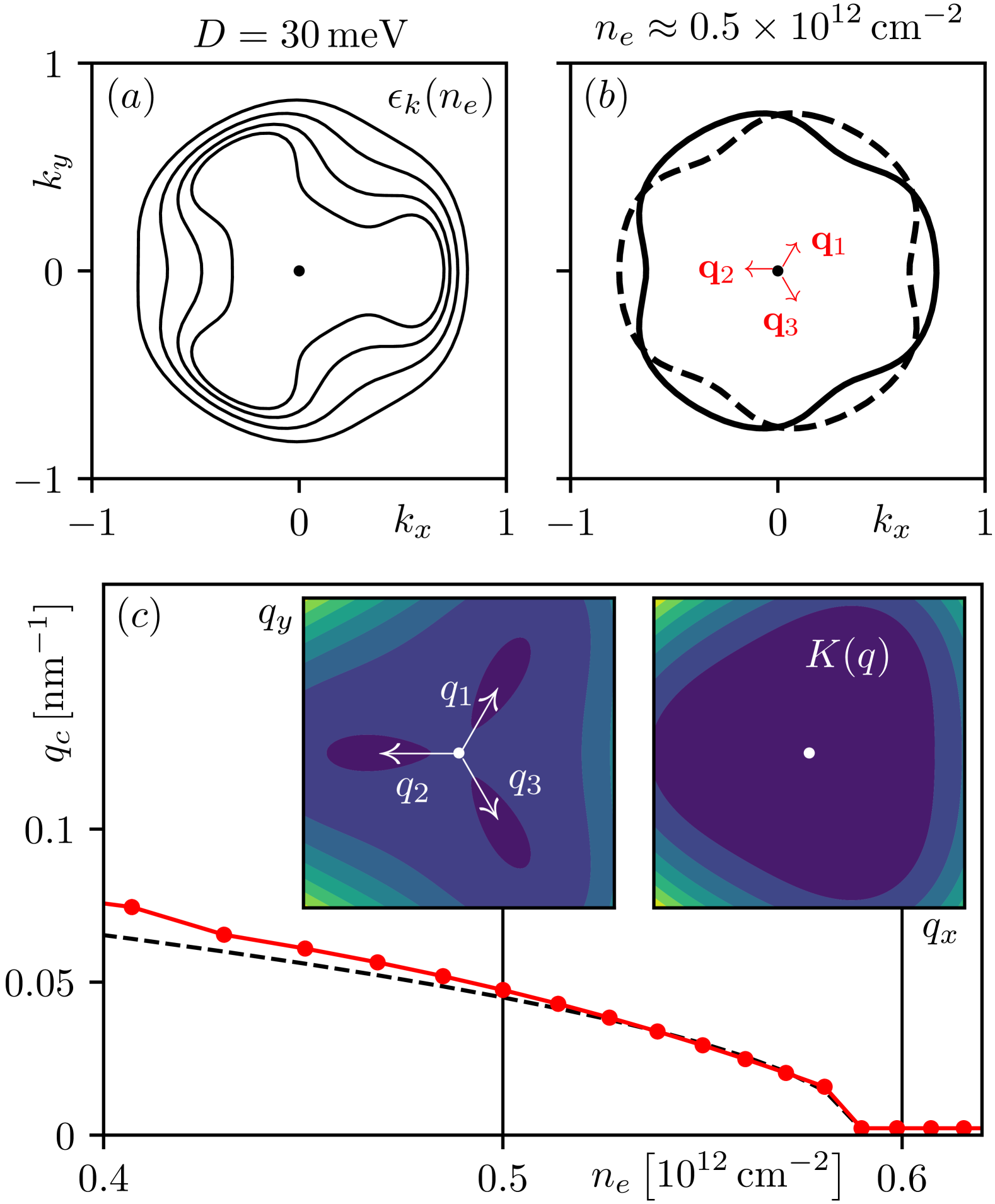
Figure 1: Finite-momentum pairing: Panel $(a)$ shows the Fermi surface in the $K$ valley, at fixed displacement field and growing electron densities $n_{e}\approx 0.2,0.4,0.5$ and $0.6\times 10^{12}\,$cm^-2. Panel $(b)$ displays the electron (solid) and hole (dashed) Fermi surfaces as well as the center-of-mass momentum shifts ${\bm{q}}_{1,2,3}$. Panel $(c)$ shows the microscopic value of $q_{0}$ (red) as a function of $n_{e}$, which displays the approximate scaling $\propto\sqrt{n_{e,0}-n_{e}}$ (dashed). Inset: colormap of $K({\bm{q}})$ for $n_{e}=0.5$ and $n_{e}=0.6\times 10^{12}\,$cm^-2.

Spontaneous vortex-antivortex lattice— We start by developing a Ginzburg-Landau (GL) theory of superconductivity in spin- and valley-polarized rhombohedral graphene based on general symmetry considerations. Full isospin polarization restricts the superconducting order parameter to have odd angular momentum $L=\pm 1$ ($p$-wave) or $\pm 3$ ($f$-wave). Moreover, the valley polarization breaks time-reversal symmetry at the orbital level, even in the absence of an external magnetic field. This lifts the degeneracy between $+L$ and $-L$ pairings, leading to a chiral superconducting state described by a single scalar order parameter [11, 10]. Finally, the valley-polarized normal state preserves three-fold rotation symmetry $C_{3z}$ of rhombohedral graphene and is invariant under the combined operation of reflection $x\rightarrow-x$ and time-reversal, $M_{x}T$. These symmetries are manifested in trigonal warping in the electronic band within a valley.

Taking into account the above symmetry constraints, the Ginzburg-Landau superconducting free energy close to the critical temperature takes the form:

$$F_{s}=\int \mathrm{d}^{2}{\bm{r}}\; \alpha(T)|\psi|^{2}+\frac{\hbar^{2}}{2m^{*}}|{\bm{D}}\psi|^{2}+\eta|{\bm{D}}^{2}\psi|^{2}$$ (1)

$$+ \gamma\psi^{*}\left(D_{x}^{3}-3D_{x}D^{2}_{y}\right)\psi+\cdots,$$

where $\alpha(T)=\alpha(0)(1-T/T_{0})$ with $\alpha(0)<0$ and ${\bm{D}}$ is the covariant derivative ${\bm{D}}=-i\nabla-(2e/\hbar){\bm{A}}$, with ${\bm{A}}$ the vector potential.

Importantly, the cubic gradient term $\propto\gamma$ (which we refer to as the cubic invariant) is allowed by (1) the presence of discrete symmetries $C_{3z}$ and $M_{x}T$, and (2) the absence of time-reversal symmetry in the valley polarized state above $T_{c}$. The quartic gradient term with $\eta>0$ is included to prevent the divergence in the gradient energy at large $\gamma$. For ${\bm{A}}=0$, it is convenient to express the quadratic coefficient $\propto|\psi|^{2}$ in the free energy in momentum space, where it takes the simple form

$$K(\bm{q})=\alpha(T)+\hbar^{2}q^{2}/2m-\gamma\,q^{3}\cos(3\theta_{\bm{q}})+\eta q^{4},$$ (2)

with the angle $\theta_{\bm{q}}$ specifying the direction of ${\bm{q}}$.

For a sufficiently large value of $\gamma>0$, the gradient term (2) has one minimum $\alpha(T)$ at $q=0$ and three degenerate minima $\alpha\equiv K({\bm{q}}_{j})$ at ${\bm{q}}_{j}$ along the directions $\theta_{j}=(2j-1)\pi/3$ with equal magnitude $|{\bm{q}}_{1}|=|{\bm{q}}_{2}|=|{\bm{q}}_{3}|\equiv q_{0}$. As a result, the free energy (1) favors finite (zero) momentum superconductivity when $\Delta\alpha=\alpha-\alpha(T)$ is negative (positive). The transition from $q=0$ to $q\neq 0$ states is first order. Our GL theory thus provides a unified description of zero- and finite-momentum states: the latter arises from an instability in gradient energy leading to a spatial modulation of the order parameter.

To determine whether finite momentum superconductivity may actually occur in rhombohedral graphene, we derive the gradient term $K({\bm{q}})$ from a microscopic calculation using the band dispersion $\epsilon_{{\bm{k}}}$ for the tetralayer graphene, with ${\bm{k}}=0$ corresponding to the Dirac point $K$. It reads

$$K({\bm{q}})=\frac{1}{2g}-\frac{k_{B}T}{2}\sum_{\omega_{n}}\int_{{\bm{k}}}|\Delta_{{\bm{k}}}|^{2}G_{p_{+}}G_{p_{-}},$$ (3)

where $\Delta_{\bm{k}}$ is the gap function which must be odd in ${\bm{k}}$: $\Delta_{-{\bm{k}}}=-\Delta_{{\bm{k}}}$; $g$ is the corresponding pairing strength; $p_{\pm}=({\bm{q}}/2\pm{\bm{k}},\pm\omega_{n})$ with $\omega_{n}=\pi(2n+1)k_{B}T$, $G_{p}=1/(i\omega_{n}-\xi_{\bm{k}})$ is the Green’s function of free electron, $\xi_{{\bm{k}}}=\epsilon_{{\bm{k}}}-\mu$ and $\int_{{\bm{k}}}=\Omega\int{d^{2}{\bm{k}}}/(2\pi)^{2}$ with $\Omega=\sqrt{3}a^{2}_{G}/2$ the unit cell area of graphene.

As is from Eq. (3), the ${\bm{q}}$ dependence in the gradient term $K({\bm{q}})$ at low temperature is largely determined by the Fermi surface of the valley-polarized normal state, shown in Fig. 1$\,(a)$. Two features are noteworthy. First, the absence of inversion symmetry $\xi_{{\bm{k}}}\neq\xi_{-{\bm{k}}}$ removes the Cooper log singularity in $\alpha(T)$ and necessitates a finite interaction strength $g$ (3) for the superconducting instability to occur, as detailed in the SM [22]. Second, the trigonal warping on the Fermi surface becomes pronounced at low density and triggers a stronger superconducting instability for finite momenta pairing at ${\bm{q}}_{j}$ due to better particle-particle nesting condition than $q=0$ pairing, as illustrated in Fig. 1$\,(b)$.

The functional form of $K({\bm{q}})$ obtained from our microscopic calculation agrees well with the GL theory (2). The absolute value of the pair center-of-mass momentum $q_{0}$ becomes nonzero below a critical density $n_{e,0}$ and increases upon further reducing the electron density, as shown in Fig. 1$\,(c)$. Therefore, we conclude that the superconducting state undergoes a first-order phase transition from being uniform to spatially modulated as the density decreases.

In the presence of pairing instability at three degenerate momenta ${\bm{q}}_{j}$ related by symmetry, the superconducting state below $T_{c}$ may be a single-${\bm{q}}$ state with a multiple-${\bm{q}}$ state, depending on the quartic terms in the free energy. Restricting to the three dominant ${\bm{q}}_{j}$ pairing components $\psi_{j}$, the free energy density takes the form

$$f_{s}=\alpha\sum_{j=1}^{3}|\psi_{j}|^{2}+\beta\sum_{j=1}^{3}|\psi_{j}|^{4}+\beta^{\prime}\sum_{i\neq j}|\psi_{i}|^{2}|\psi_{j}|^{2}.$$ (4)

The microscopic calculation of the quartic coefficients gives:

$$\begin{split}&\beta=\frac{k_{B}T}{4}\sum_{\omega_{n}}\int_{{\bm{k}}}|\Delta_{{\bm{k}}}|^{4}G_{p_{+}}^{2}G_{p_{-}}^{2},\\ &\beta^{\prime}=\frac{k_{B}T}{2}\sum_{\omega_{n}}\int_{{\bm{k}}}|\Delta_{{\bm{k}}+{\bm{q}}_{j}/2}|^{2}|\Delta_{{\bm{k}}+{\bm{q}}_{l}/2}|^{2}G^{2}_{p_{1}}G_{p_{2}}G_{p_{3}},\\ \end{split}$$ (5)

where $p_{\pm}$ have been defined below Eq. (3), and, in the integral for $\beta^{\prime}$, $p_{1}=({\bm{k}}+({\bm{q}}_{j}+{\bm{q}}_{l})/2,\omega_{n})$, $p_{2,3}=(\pm({\bm{q}}_{l}-{\bm{q}}_{j})/2-{\bm{k}},-\omega_{n})$. Performing the integrals in Eq. (5), we found that $\beta>\beta^{\prime}>0$, as shown in the SM [22], indicating that the triple-${\bm{q}}$ state characterized by an equal superposition of ${\bm{q}}_{1,2,3}$ components is favored over a wide a range of parameters. Its order parameter is

$$\psi=|\psi_{c}|\left(e^{i{\bm{q}}_{1}\cdot{\bm{r}}}+e^{i{\bm{q}}_{2}\cdot{\bm{r}}}+e^{i{\bm{q}}_{3}\cdot{\bm{r}}}\right),$$ (6)

with $|\psi_{c}|=\sqrt{|\alpha|/(2\beta+4\beta^{\prime})}$ found by minimizing Eq. (4). Note that the relative phases of the three components (6) are removed by a gauge transformation involving the global phase of the order parameter and a translation of coordinates [22].

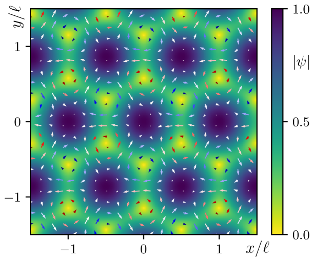
Figure 2: Vortex-antivortex lattice: Order parameter modulus (colormap) and current/phase pattern (arrows) associated to spontaneous VAL state (6). The coloring of the current arrows reflects the local winding of the order parameter, red for vortex and blue for anti-vortex.

The spatial profile of the modulus and the phase of the triple-${\bm{q}}$ order parameter are shown in Fig. 2. Due to the interference between the three plane-wave components, the order parameter exhibits periodic modulation with a large period $\ell=4\pi/(3q_{0})$ and a honeycomb lattice structure. Furthermore, $\psi$ has two sets of nodes with $\pm 2\pi$ phase winding around them, which are located at two triangular sublattices ${\bm{v}}^{\pm}_{n,m}=n{\bm{a}}_{1}+m{\bm{a}}_{2}\pm{\bm{u}}$, where $n,m\in\mathbb{Z}$, ${\bm{a}}_{1/2}=\ell\left(\pm 1/2,\sqrt{3}/2\right)$, ${\bm{u}}=\ell\left(0,1/\sqrt{3}\right)$. Together, these form a honeycomb lattice of vortices and antivortices, spontaneously formed at zero magnetic field. Therefore, we call this spatially modulated superconducting state a vortex-antitex lattice (VAL) state. The VAL state should be contrasted with other types of finite momentum superconductivity, such as Fulde-Ferrell state with a constant modulus or the Larkin-Ovchinnikov state with a real order parameter.

Experimental manifestation – The VAL state exhibits spontaneous circulating supercurrents and therefore produces a spatially varying magnetic field texture, which can be imaged with SQUID-on-tip scanning techniques [23, 24]. Using $j\sim e(n_{e}/d)(\hbar\,q_{0}/m)\sim 10^{4}\,$A/cm^-2 as an estimate [25] of the current density circulating in the VAL state ($n_{e}\sim 10^{12}\,\text{cm}^{-2}$ is the $2$D electron density, $m$ taken to be the bare electron mass and $d\sim 1\,$nm the sample thickness) we find magnetic fields $B\sim(4\pi/c)jd$ in the order of $10^{-4}\,$mT, well within the sensitivity range of the experimental technique.

The spatial varying order parameter in VAL phase at zero applied magnetic field displays a single characteristic length scale $\ell$, in contrast with a traditional Abrikosov vortex lattice where the ratio of the vortex core size $\sim\xi$ to the lattice constant $\propto\sqrt{1/H}$ can be tuned by means of the external magnetic field. Nonetheless, in both the VAL and the Abrikosov lattice, an electric current can induce the (thermally assisted) motion of the vortices, creating an electric field inside the superconductor and leading to finite resistivity [26]. This is particularly relevant for rhombohedral graphene, where the interface between different orbital magnetic domains (time-reversed copies where $\gamma,{\bm{q}}_{i},\psi\to-\gamma,-{\bm{q}}_{i},\psi^{*}$) act as grain boundaries that can facilitate vortex motion.

In light of our theory, we now examine experimental data on rhombohedral graphene. We note that an anomalous region exists at densities $n_{e}\sim 0.4-0.6\times 10^{12}\,$cm^-2, below SC-1 and above the highly insulating Wigner crystal. Here, the resistivity drops rapidly below a critical temperature (comparable to $T_{c}$ of SC-1 at slightly higher density) and saturates to a small nonzero value at low temperature, shown in Fig. 3. This unusual behavior, unaddressed in Ref.[1], is naturally explained by the flux-flow resistance in our VAL state. Drawing on the Bardeen-Stephen formula [27], we estimate the flux-flow resistivity to be a fraction $(q_{0}\,\xi)^{2}\sim 5-10\,\%$ of the normal-state $R_{n}$, with $\xi\approx 20\,$nm taken from Ref. [1]. This explains the low-temperature plateau observed at zero field (panel $(a)$). Further evidence for identifying this region as the VAL state is provided by its response to an out-of-plane magnetic field, as will be shown below.

VAL under out-of-plane magnetic field – We now proceed to discuss the response of the VAL state in rhombohedral graphene to an out-of-plane magnetic field. Conventional $q=0$ superconductivity is destroyed at $H_{c2}=\Phi_{0}/(2\pi\xi^{2})$ when vortices strongly overlap. However, for the VAL state, a small magnetic field $\sim\phi_{0}q_{0}^{2}$ is enough to penalize the energetics of the VAL and induce a first order phase transition into the conventional superconducting state, as we will now show.

This transition is marked by a change in the spatial profile of the order parameter driven by the magnetic field. To estimate the occurrence of the transition, we can account for the effect of $H$ via a momentum shift of the order of the inverse magnetic length $\ell_{B}^{-1}=\sqrt{\phi_{0}/2\pi H}$. Imposing that $K(q_{0}+\ell_{B}^{-1})$ is equal to the barrier $\sim\eta q_{0}^{4}$ separating the finite- and zero-momentum states, and using that the curvature of $K({\bm{q}})$ around ${\bm{q}}_{i}$ scales with $\eta q_{0}^{2}$ (cf SM [22]), we then find that $H_{c}\sim\phi_{0}q_{0}^{2}$. Using the dependence of $q_{0}$ on the electron density shown from Fig. 1$\,(c)$, we find the critical field displays an approximate linear scaling with $n_{e0}-n_{e}$; this result reproduces the observed phase boundary in Fig. 3$\,(b)$.

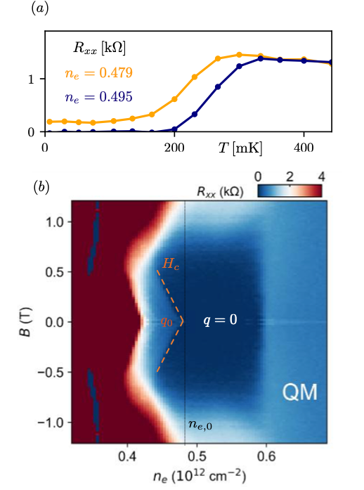
Figure 3: Experimental phase diagram [1]: $(a)$ Temperature dependence of the longitudinal resistivity in the VAL (orange) and zero-momentum state (blue) when $H=0$. In the VAL state (orange), $R_{xx}$ saturates to a plateau determined by the vortex-antivortex motion. $(b)$ At small temperatures and electronic densities $\lesssim 0.48\times 10^{-12}\,$cm^-2, the system is in the VAL phase (finite resistivity) for small magnetic fields and jumps into the zero-momentum state (vanishing resistivity) going across the $H_{c}$ line (orange dashed). For larger fields, the finite-momentum state is metastable and the system prefers the zero-momentum state until the superconductivity vanishes smoothly.

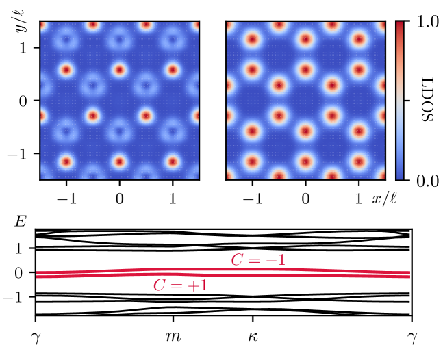
Figure 4: Majorana zero-modes: Local density of states for the upper Majorana band as measured by a local STM probe. As expected for a topological superconductor, the MZMs are concentrated in the cores of the VAL. Lower panel: energy dispersion of the BdG bands, expressed in units of the gap. The Majorana bands (red lines) are in gap states with Chern number $C=\pm 1$ and energy spacing $\sim W$.

Majoranas and Pomeranchuk effect – Topological superconductors host Majorana zero-modes (MZMs) inside their vortex cores [6, 7]. These exotic particles manifest themselves as in-gap states with zero energy and display non-Abelian statistics, thus holding the promise to fault-tolerant topological quantum computing [9]. Inspired by the presence of a spontaneous VAL inside our system, we derive a microscopic Bogoliubov-de Gennes Hamiltonian $h_{\text{BdG}}$ for the VAL phase [28, 29, 30, 31, 32, 22] which in the Nambu basis $(\Psi,\Psi^{\dagger})$ reads:

$$h_{\rm BdG}({\bm{r}})=\begin{pmatrix}\xi_{-i\nabla}&\{\psi({\bm{r}}),-i\bar{\partial}\}/2\\ h.c.&-\xi_{i\nabla}\end{pmatrix},$$ (7)

where $\bar{\partial}=\partial_{x}+i\partial_{y}$ and $\xi_{-i\nabla}=\epsilon_{-i\nabla}-\mu$.

The spectrum of the Hamiltonian $h_{\text{BdG}}$ is influenced by the order parameter $\psi({\bm{r}})$. For a single-$q$ condensate $|\psi({\bm{r}})|$ is constant and the quasiparticle spectrum is generically gapped with the exceptions of nodal configurations where electron-hole surfaces intersect at ${\bm{k}}=0$. On the other hand, in the VAL, $|\psi({\bm{r}})|$ is spatially modulated and vanishes as $\psi({\bm{r}}+\bm{v}_{n,m}^{+})\propto z$ and $\psi({\bm{r}}+\bm{v}_{n,m}^{-})\propto z^{*}$ with $z=x+iy$ around the vortices and antivortices, respectively, forming the honeycomb lattice in Fig. 2. In proximity of these nodes, Majorana zero-modes are realized [6]. The periodic array characterizing the VAL gives rise to in-gap flat bands of Majorana fermions (red lines in lower panel Fig. 4) with Chern number $C=\pm 1$.

The corresponding local density of state (LDOS) is concentrated inside the cores of the VAL, as shown in Fig. 4. The two panels display the LDOS measured as by an STM probe at small positive bias, at zero and finite temperatures. In the zero-temperature case, quasi-particles fill all the BdG bands with negative energies and electrons can only tunnel in the superconductor via the particle sector of the positive Majorana band. The resulting LDOS then distinguishes between vortices and antivortices [33] (Fig. 4$\,(a)$). When the temperature is larger than the Majorana bands spacing $\sim W$, on the other hand, band occupation is approximately symmetric and the electrons can tunnel as a particles in the upper band and holes in the lower band, resulting in a symmetric LDOS (Fig. 4$\,(b)$).

Remarkably rich physics emerges upon considering the physics of Majorana zero-modes at finite-temperatures. Because of MZMs, a spontaneous VAL with $2N$ vortex cores has a $2^{N}$-fold degeneracy [7], giving rise to an entropic contribution to the superconducting free energy that scales as $-TN\log 2\sim-T(\mathcal{A}/\mathcal{A}_{\rm uc})$ and is extensive in the sample area $\mathcal{A}$. At finite temperatures, the MZMs therefore give rise to a Pomeranchuk effect [34] that reduces the free energy of the VAL state, further stabilizing it against other possible order parameter configurations. While this effect was previously observed in magic-angle twisted graphene [35, 36], where it is of magnetic origin, the topological root of the Pomeranchuk effect in rhombohedral graphene makes it unprecedented.

Discussion – Spin and valley polarized superconductors are one of the most fascinating and challenging phases recently realized in multilayer graphene materials [1]. Our work presents a new state of matter, the vortex-antivortex lattice (VAL), characterized by honeycomb lattice geometry and hosting low-energy Majorana flat bands. In the low-electron-density regime of rhombohedral graphene, our microscopic calculations demonstrate that trigonal warping favors a finite center-of-mass momentum, while the quartic term selects an equal superposition of the three condensates related by threefold rotational symmetry. This superposition features nodes on an honeycomb lattice with sublattices featuring opposite vorticity and, therefore, realizes in-gap flat bands of Majorana fermions.

The VAL shows a number of phenomenological properties in good agreement with the recent observations [1]. First, a current flowing in the sample induces motion of vortices and antivortices resulting in a finite residual resistance. Second, an out-of-plane magnetic field induces a first-order transition from the VAL to a uniform superconductor, consistent with the observation of a zero-resistance state stabilized at finite field. Finally, our theory predicts a Pomeranchuk effect arising from low-energy in-gap Majorana flat bands, which further stabilizes the VAL phase over the uniform superconductor as temperature increases. We propose real-space imaging via STM to detect Majorana fermions and SQUID to visualize the lattice of vortex-antivortex pairs. Another smoking gun evidence of the VAL is the optical phonon mode [37, 38] associated with the relative shift of one sublattice with respect to the other. Finally, we hope that our work will motivate experimental efforts to directly image the magnetic texture resulting from the spontaneous vortex-antivortex lattice, for example with the SQUID-on-tip scanning technique.

Acknowledgments – It is our pleasure to thank Long Ju and Tonghang Han for insightful discussions and providing us the experimental figures used in this work. We also thank Yoichi Ando for a stimulating remark about Ref. [1] and Max Geier for discussion in the early stage of this work. This work was supported by a Simons Investigator Award from the Simons Foundation. F.G. is grateful for the financial support from the Swiss National Science Foundation (Postdoc.Mobility Grant No. 222230).

These supplementary materials contain the details of the Ginzburg-Landau theory as well as microscopic calculations supporting the results presented in the main text. Sec. A and A.1 contain details on the symmetry-constrainted expression of the particle-particle correlation function $K({\bm{q}})$. In Sec. B we show that the order parameter of the VAL is unambiguously determined, i.e. any additional phase in the Fourier components $\psi_{j}=|\psi_{c}|\to|\psi_{c}|e^{i\varphi_{j}}$ is absorbed by a gauge transformation. Sec. C and Sec. C.1 provide microscopic results establishing a solid ground for our theory. The continuum model Hamiltonian for the VAL is discussed in Sec. C.2.

Appendix A Scaling properties and phase diagram of the quadratic kernel $K(q)$

In this section we want to determine the phase diagram associated to the quadratic kernel

$$K(q)=\alpha(T)+\left(\hbar^{2}/2m^{*}\right)q^{2}-\gamma\,q^{3}+\eta q^{4}.$$ (1)

First, we want to reduce the parameter space by introducing the momentum scale $q_{c}=\sqrt{\hbar^{2}/2m^{*}\eta}$ and the dimensionless variable $t=q/q_{c}$, such that

$$\Delta K(q)=\eta\left(\frac{\hbar^{2}}{2m^{*}\eta}\right)^{2}t^{2}+\gamma\left(\frac{\hbar^{2}}{2m^{*}\eta}\right)^{3/2}t^{3}+\eta\left(\frac{\hbar^{2}}{2m^{*}\eta}\right)^{2}t^{4}\implies\frac{\Delta K(q)}{\eta q_{0}^{4}}=t^{2}-2(\gamma/\gamma_{\rm cx})t^{3}+t^{4},$$ (2)

after introducing $\gamma_{\rm cx}=2\sqrt{\hbar^{2}\eta/2m^{*}}$. We therefore see that $\Delta K(q)=K(q)-K(0)$ scales $\propto\eta q_{c}^{4}$.

The minima of (2) are located at

$$2t-6(\gamma/\gamma_{\rm cx})t^{2}+4t^{3}=0\implies t=0\quad\text{and}\quad t_{0}=\frac{q_{0}}{q_{c}}=\frac{3}{4}\left(\frac{\gamma}{\gamma_{\rm cx}}\pm\frac{\sqrt{\gamma^{2}-\gamma_{\rm sp}^{2}}}{\gamma_{\rm cx}}\right),$$ (3)

where $\gamma_{\rm sp}=(4/3)\sqrt{\hbar^{2}\eta/m^{*}}=\sqrt{8}\gamma_{\rm cx}/3$. We have therefore found that the finite momentum solution exits only above the spinodal line $\gamma=\gamma_{\rm sp}$. Along this line $t_{0}=1/\sqrt{2}$, while, for $\gamma=\gamma_{\rm cx}$, the solution is $t_{0}=1$. Plugging this into Eq. (2), one finds that $\Delta K(t_{0}=1)=0$: we can therefore identify $\gamma_{\rm cx}$ with the coexistence line where $\Delta\alpha=0$.

A.1 Curvature and anisotropy of $K(q)$ around $q_{i}$

The kernel $K({\bm{q}})$ can be expanded around ${\bm{q}}_{i}$ with the help of the coefficients

$$C_{\parallel}=\left(\hbar^{2}/2m^{*}\right)-3q_{0}(\gamma-2\eta q_{0}),\quad C_{\perp} =\left(\hbar^{2}/2m^{*}\right)+q_{0}(3\gamma+2\eta q_{0}),$$ (4)

that one finds by expanding $K({\bm{q}})$ to quadratic order around ${\bm{q}}_{i}$ (using that $q^{3}\cos 3\theta_{\bm{q}}=q_{x}^{3}-3q_{x}q_{y}^{2}$). We remark that $C_{\perp}>C_{\parallel}$ always holds.

For the sake of simplicity, it is convenient to work with the combination

$$\bar{C}=\frac{C_{\perp}+C_{\parallel}}{2}=\frac{\hbar^{2}}{2m^{*}}+4\eta q_{0}^{2},\quad\gamma=\frac{C_{\perp}-C_{\parallel}}{2\bar{C}}=\frac{3\gamma q_{0}-2\eta q_{0}^{2}}{\hbar^{2}/2m^{*}+4\eta q_{0}^{2}},$$ (5)

as done in the main text. In terms of the rescaled variable introduced in the previous section, the coefficients of Eqs. (4) and (5) read

$$\frac{C_{\parallel}}{\eta q_{c}^{2}}=1-6t_{0}\left(\frac{\gamma}{\gamma_{\rm cx}}-t_{0}\right),\quad\frac{C_{\perp}}{\eta q_{c}^{2}}=1+6t_{0}\left(\frac{\gamma}{\gamma_{\rm cx}}+\frac{t_{0}}{3}\right),\quad\frac{\bar{C}}{\eta q_{c}^{2}}=1+4t_{c}^{2},$$ (6)

and

$$a=\frac{6(\gamma/\gamma_{\rm cx})t_{0}-2t_{0}^{2}}{1+4t_{0}^{2}}.$$ (7)

We see that the coefficients $C_{\parallel},C_{\perp},\bar{C}$ scale with $\eta q_{c}^{2}$, while $a$ depends only on $\gamma/\gamma_{\rm cx}$ and changes from $a(\gamma_{\rm sp})=1$ to $a(\gamma_{\rm cx})=4/5$ and $a(\gamma\gg\gamma_{\rm sp})\approx 1/2$ upon increasing the cubic term $\gamma/\gamma_{\rm cx}$.

Appendix B Generality of the order parameter

Consider the combination of three condensates with distinct center-of-mass momenta ${\bm{q}}_{j}=q_{0}\,\hat{\bm{e}}(\theta_{j})$

$$\psi=\sum_{j=1}^{3}\psi_{j}e^{i{\bm{q}}_{j}\cdot{\bm{r}}},$$ (8)

with $|\psi_{j}|=|\psi_{c}|$. Here, we show that the three phases $\varphi_{j}=\arg\psi_{j}$ do not play a physical role and can be absorbed into a redefinition of the global phase of the condensate and in a translation of the origin of the vortex lattice. The combination of these transformations correspond to:

$$\psi({\bm{r}})\to\psi({\bm{r}}+{\bm{d}})e^{i\chi}=|\psi_{c}|e^{i\chi}\left[e^{i\varphi_{1}}e^{i{\bm{q}}_{1}\cdot({\bm{r}}+{\bm{d}})}+e^{i\varphi_{2}}e^{i{\bm{q}}_{2}\cdot({\bm{r}}+{\bm{d}})}+e^{i\varphi_{3}}e^{i{\bm{q}}_{3}\cdot({\bm{r}}+{\bm{d}})}\right].$$ (9)

By choosing the translation vector ${\bm{d}}$ as

$${\bm{d}}=-\left[\left(\frac{\varphi_{1}+\chi}{2\pi}\right){\bm{a}}_{1}+\left(\frac{\varphi_{2}+\chi}{2\pi}\right){\bm{a}}_{2}\right],$$ (10)

with ${\bm{a}}_{j}$ such that ${\bm{a}}_{j}\cdot{\bm{q}}_{l}=2\pi\delta_{jl}$ and $j,l=1,2$. The order parameter then becomes

$$\psi({\bm{r}})\to\psi({\bm{r}}+{\bm{d}})e^{i\chi}=|\psi_{0}|\left[e^{i{\bm{q}}_{1}\cdot{\bm{r}}}+e^{i{\bm{q}}_{2}\cdot{\bm{r}}}+e^{i{\bm{q}}_{3}\cdot r+i\left(3\chi+\sum_{l=1}^{3}\varphi_{l}\right)}\right].$$ (11)

Finally, by choosing the global phase $\chi$ as

$$\chi=\frac{2\pi}{3}n-\frac{\varphi_{1}+\varphi_{2}+\varphi_{3}}{3},\quad\quad\text{with }n\in\mathbb{Z},$$ (12)

with $n\in\mathbb{Z}$ which concludes the proof. We remark that the global phase $\chi$ corresponds to the Goldstone mode associated with the phase of the superconducting order. In contrast, $\varphi_{2,3}$ represent phononic modes arising from the spontaneous breaking of translational symmetry.

Appendix C Microscopic Modeling

In this section, we discuss the microscopic model employed to describe tetralayer graphene.

C.0.1 Tight-binding model

We use the lattice model for describing tetra-layer rhombohedral graphene [39, 21]:

$$h=\begin{pmatrix}h^{(0)}_{1}&h^{(1)}&h^{(2)}&0\\ h^{(1)\dagger}&h^{(0)}_{2}&h^{(1)}&h^{(2)}\\ h^{(2)\dagger}&h^{(1)\dagger}&h^{(0)}_{3}&h^{(1)}\\ 0&h^{(2)\dagger}&h^{{(1)}\dagger}&h^{(0)}_{4}\end{pmatrix},$$ (13)

where for simplicity we dropped the momentum dependency, $u_{\ell}=D(\ell-(N+1)/2)$ and:

$$h^{(0)}_{l}({\bm{k}})=\begin{pmatrix}u_{l}&-t_{0}f_{{\bm{k}}}\\ -t_{0}f^{*}_{{\bm{k}}}&u_{l}\end{pmatrix},\quad h^{(1)}({\bm{k}})=\begin{pmatrix}t_{4}f_{{\bm{k}}}&t_{3}f^{*}_{{\bm{k}}}\\ t_{1}&t_{4}f_{{\bm{k}}}\end{pmatrix},\quad h^{(2)}=\begin{pmatrix}0&t_{2}/2\\ 0&0\end{pmatrix},\quad f_{{\bm{k}}}=\sum^{3}_{j=1}e^{i\bm{u}_{j}\cdot{\bm{k}}}.$$ (14)

In the latter expression, we have introduced the vectors connecting the two sublattices $\bm{\delta}_{j}=a_{G}\mathcal{R}^{j-1}_{2\pi/3}(0,1)/\sqrt{3}$ and $a_{G}=0.246$nm. Model parameters taken from [40] are $t_{0}=3.1$eV, $t_{1}=380$meV and $(t_{2},t_{3},t_{4})=(-21,290,141)$meV and $u_{l}$ intralayer potential reflecting the displacement field. The model features a characteristic length scale $\ell=\hbar v_{F}/t_{1}=a_{G}\sqrt{3}t_{0}/(2t_{1})\approx 7a_{G}\approx 2$nm.

C.0.2 Interaction

Our low energy theory is constructed employing valley and spin-polarized electrons with dispersion $\epsilon_{{\bm{k}}}$ of the conduction band of tetra-layer graphene (13):

$$H_{0}=\sum_{{\bm{k}}}\epsilon_{{\bm{k}}}c^{\dagger}_{{\bm{k}}}c_{{\bm{k}}}.$$ (15)

Furthermore, we employ a finite range attractive interaction:

$$H_{\rm int}=\frac{1}{2}\sum_{i\neq j}V({\bm{r}}_{i}-{\bm{r}}_{j}),$$ (16)

where $V({\bm{r}})=-V_{0}e^{-r^{2}/(2a^{2})}$ and in momentum space $V_{{\bm{q}}}=-2\pi a^{2}V_{0}e^{-{\bm{q}}^{2}a^{2}/2}$. In second quantization, we have:

$$H_{\rm int}=\frac{1}{2A}\sum_{{\bm{q}}{\bm{k}}{\bm{k}}^{\prime}}V_{{\bm{k}}^{\prime}-{\bm{k}}}c^{\dagger}_{{\bm{k}}+\frac{{\bm{q}}}{2}}c^{\dagger}_{\frac{{\bm{q}}}{2}-{\bm{k}}}c_{\frac{{\bm{q}}}{2}-{\bm{k}}^{\prime}}c_{{\bm{k}}^{\prime}+\frac{{\bm{q}}}{2}},$$ (17)

where we have introduced:

$$V_{{\bm{k}}^{\prime}-{\bm{k}}}=-2\pi a^{2}V_{0}e^{-a^{2}({\bm{k}}-{\bm{k}}^{\prime})^{2}/2}.$$ (18)

Employing the Jacobi-Anger expansion we find:

$$V_{{\bm{k}}^{\prime}-{\bm{k}}}=-2\pi a^{2}V_{0}e^{-a^{2}k^{2}/2}e^{-a^{2}k^{\prime 2}/2}\sum_{n=-\infty}^{\infty}I_{n}(kk^{\prime}a^{2})e^{in\theta}e^{-in\theta^{\prime}},$$ (19)

where $I_{n}(x)$ is the modified first Bessel function. In the limit of short-ranged attraction $|kk^{\prime}a^{2}|\ll 1$ and we find:

$$I_{n}(kk^{\prime}a^{2})\approx\frac{(kk^{\prime}a^{2})^{n}}{2^{n}n!}.$$ (20)

The latter expansion is justified when the interaction range $a$ is smaller than the characteristic interparticle separation $d=1/\sqrt{n_{e}}\approx 10$ nm determining the relevant momentum scale. Keeping only the leading contribution to the momentum expansion:

$$V_{{\bm{k}}^{\prime}-{\bm{k}}}\approx-\pi a^{2}V_{0}\sum_{n=\pm}({\bm{k}}_{n}a)({{\bm{k}}^{\prime}}_{n}^{*}a)=-\pi a_{G}^{2}(a/a_{G})^{4}V_{0}\sum_{n=\pm}({\bm{k}}_{n}a_{G})({{\bm{k}}^{\prime}}_{n}^{*}a_{G}).$$ (21)

Without losing generality, in the following we perform calculations keeping the general structure $V_{{\bm{k}},{\bm{k}}^{\prime}}=-g\Delta_{{\bm{k}}}\Delta_{{\bm{k}}^{\prime}}^{*}$ with $\Delta_{{\bm{k}}}$ gap function. We then perform specific toy model calculations under the assumption that the normal state favors $p$-wave symmetry with a well-defined chirality, characterized by$L_{z}=\pm 1$ depending on the valley $K/K^{\prime}$ [11]. The interaction takes the form $V_{{\bm{k}}^{\prime}-{\bm{k}}}=-g{\bm{k}}_{\pm}{{\bm{k}}}^{\prime}_{\mp}$ with $g=\pi(a/a_{G})^{4}a_{G}^{2}V_{0}$.

C.1 Derivation of the Ginzburg-Landau theory

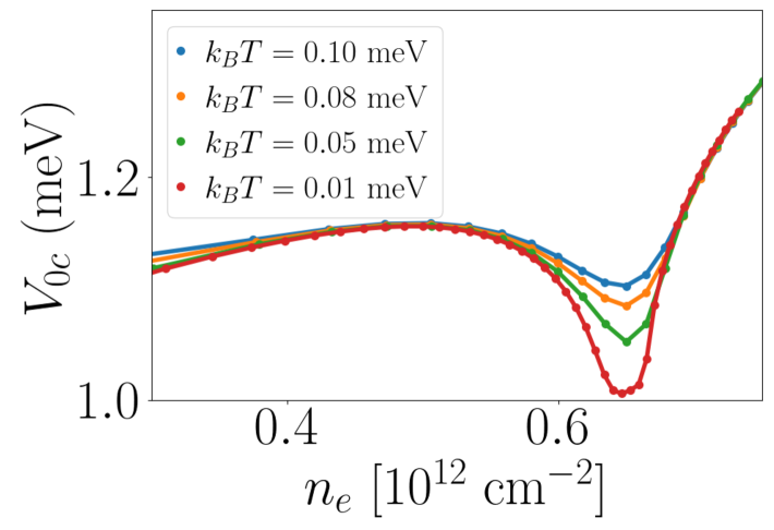
Figure S1: Critical coupling strength $V_{0c}$ (26) as a function of the temperature for different carrier concentrations and $D=30$meV.

The action describing the effective theory $H=H_{0}+H_{\rm int}$ reads:

$$S=\int^{\beta}_{0}d\tau\left[\sum_{{\bm{k}}}c^{\dagger}_{{\bm{k}}}(\partial_{\tau}-\xi_{{\bm{k}}})c_{{\bm{k}}}+\frac{1}{2}\sum_{{\bm{q}}{\bm{k}}}\psi({\bm{q}})\Delta_{{\bm{k}}}c^{\dagger}_{{\bm{k}}+{\bm{q}}/2}c^{\dagger}_{{\bm{q}}/2-{\bm{k}}}+h.c.+A\sum_{{\bm{q}}}\frac{|\psi({\bm{q}})|^{2}}{2g}\right],$$ (22)

where $\xi=\epsilon-\mu$, $\psi({\bm{q}})$ is the Hubbard-Stratonovich field associated to the pairing field and $\Delta_{{\bm{k}}}$ the gap function $\Delta_{-{\bm{k}}}=-\Delta_{{\bm{k}}}$. We integrate the fermions and expand the theory to second order in the pairing field $\psi({\bm{q}})$:

$$F^{(2)}_{\psi}=A\sum_{{\bm{q}}}\frac{|\psi({\bm{q}})|^{2}}{2g}-\frac{T}{2}\sum_{{\bm{q}}}|\psi({\bm{q}})|^{2}\sum_{\omega_{n}}\int_{{\bm{k}}}|\Delta_{\bm{k}}|^{2}G({\bm{k}}+{\bm{q}}/2,\omega_{n})G({\bm{q}}/2-{\bm{k}},-\omega_{n})=\sum_{{\bm{q}}}\psi({\bm{q}})^{*}K({\bm{q}})\psi({\bm{q}}),$$ (23)

where $\omega_{n}=i\pi(2n+1)k_{B}T$, $G^{-1}({\bm{k}},\omega_{n})=(i\omega_{n}-\xi_{{\bm{k}}})$ and we have introduced $K({\bm{q}})$ shown in Fig. S3a) and given by:

$$K({\bm{q}}) =\frac{1}{2g}-\frac{T}{2}\sum_{\omega_{n}}\int_{{\bm{k}}}|\Delta_{\bm{k}}|^{2}G\left({\bm{k}}+\frac{{\bm{q}}}{2},\omega_{n}\right)G\left(\frac{{\bm{q}}}{2}-{\bm{k}},-\omega_{n}\right)$$

$$=\frac{1}{2g}-\frac{\Omega}{4}\int\frac{d^{2}{\bm{k}}}{(2\pi)^{2}}\frac{|\Delta_{\bm{k}}|^{2}}{\xi_{{\bm{q}}/2+{\bm{k}}}+\xi_{{\bm{q}}/2-{\bm{k}}}}\left(\tanh\frac{\xi_{{\bm{q}}/2+{\bm{k}}}}{2k_{B}T}+\tanh\frac{\xi_{{\bm{q}}/2-{\bm{k}}}}{2k_{B}T}\right),$$ (24)

where $\Omega=|\bm{a}_{1}\times\bm{a}_{2}|=\sqrt{3}a^{2}_{G}/2$ is the area of the unit cell. By symmetry arguments, for a small center-of-mass momenta we can expand $K({\bm{q}})$ to find Eq. (2) in the main text. The latter expansion accurately describes the numerical results, as shown by the fit in Fig. 3.

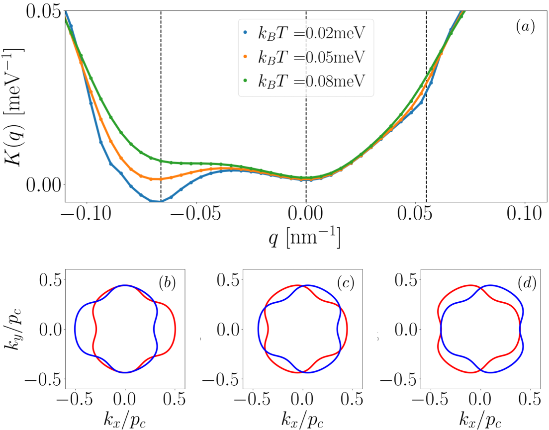
Figure S2: Panel $(a)$ shows $K({\bm{q}})$ along $q_{x}$ for different temperatures at filling factor $n=0.45\times 10^{12}$cm^-2 and $D=30$meV. We employed $V_{0}=1.15$meV and $a=20a_{G}$. Panels $(b)$, $(c)$ and $(d)$ show the electrons (red) and hole (blue) Fermi surface with net center-of-mass momenta ${\bm{q}}$ correspondent to the three dashed vertical lines in panel $(a)$. Momenta are measured in unit of $p_{c}=t_{1}/\hbar v_{F}$.

We emphasize that the absence of the Cooper log singularity requires that the coupling constant $g$ is larger than a critical threshold in order for the superconductivity to take place. We provide an estimate of the critical coupling strength $g_{c}$ for ${\bm{q}}=0$ superconductivity, defined as $K({\bm{q}}=0)=0$:

$$g_{c}(T,n_{e})=\left[\frac{\Omega}{2}\int\frac{d^{2}{\bm{k}}}{(2\pi)^{2}}\frac{|\Delta_{\bm{k}}|^{2}}{\xi_{{\bm{k}}}+\xi_{-{\bm{k}}}}\left(\tanh\frac{\xi_{{\bm{k}}}}{2k_{B}T}+\tanh\frac{\xi_{-{\bm{k}}}}{2k_{B}T}\right)\right]^{-1},$$ (25)

where the numerical analysis has been performed utilizing the form factor $\Delta_{\bm{k}}=k_{x}+ik_{y}$ characteristic of a chiral $p$-wave superconductor [6]. Exploiting the relation in Eq. 21, we find that the critical interaction strength reads:

$$V_{0c}(T,n_{e})=\frac{a^{2}_{G}g(T,n_{e})}{\pi a^{4}}.$$ (26)

Fig. S1 displays $V_{0c}$ as a function of the filling factor for different values of the temperature where we set $a=20a_{G}\approx 5$nm which remains smaller than the interparticle separation $d\geq 10$nm.

Fig. S2$(a)$ shows the evolution of $K({\bm{q}})$ for different values of the temperature at filling factor $n_{e}=0.45$. Figs. S2$(b)$, $(c)$ and $(d)$ depict the electron $\xi_{{\bm{q}}/2-{\bm{k}}}$ and hole $-\xi_{{\bm{q}}/2-{\bm{k}}}$ Fermi surfaces for three different center-of-mass shifts ${\bm{q}}$. The resonant condition is achieved for Fig. S2$(a)$ where the Cooper pair has net center-of-mass momentum ${\bm{q}}_{1}$. We remark that this condition is also achieved for the $C_{3z}$ symmetric momenta ${\bm{q}}_{2}=C_{3z}{\bm{q}}_{1}$ and ${\bm{q}}_{3}=C^{2}_{3z}{\bm{q}}_{1}$.

Figure S3: Panel a) shows the bubble diagram for the quadratic part $K({\bm{q}})$ of the superconducting action. Panels b) and c) show the box diagrams for the $|\psi|^{4}$ contribution to the free energy, with $j=l$ in b) and $j\neq l$ in c). Incoming and outgoing wavy lines are $\psi^{*}({\bm{q}}_{j/l})$ and $\psi({\bm{q}}_{j/l})$, respectively. Each vertex $\Delta_{{\bm{k}}}$ carries momentum given by the difference between the momenta of the incoming and outgoing fermionic lines.

To differentiate between different finite momentum condensates, we calculate the quartic contribution $\propto|\psi|^{4}$ to the action of the paring field. This is expressed in terms of box diagrams that includes 4 vertices and 4 internal legs. Each vertex carries a momentum label ${\bm{q}}_{j}$ with $j=1,2,3$. Particle number conservation implies that out of 4 vertices two are $\psi^{*}({\bm{q}}_{j_{1/3}})$ and the other two $\psi({\bm{q}}_{j_{2/4}})$. Finally, momentum conservation enforces ${\bm{q}}_{j_{1}}+{\bm{q}}_{j_{3}}={\bm{q}}_{j_{2}}+{\bm{q}}_{j_{4}}$. To start with, we consider the diagonal contribution where ${\bm{q}}_{j_{1}}={\bm{q}}_{j_{3}}$ and, therefore, ${\bm{q}}_{j_{2}}={\bm{q}}_{j_{4}}$. The resulting contribution is shown in Fig. S3b) and reads:

$$\beta=\frac{T}{4}\sum_{\omega_{n}}\int_{{\bm{k}}}|\Delta_{\bm{k}}|^{4}G\left(\frac{{\bm{q}}_{j}}{2}+{\bm{k}},\omega_{n}\right)^{2}G\left(\frac{{\bm{q}}_{j}}{2}-{\bm{k}},-\omega_{n}\right)^{2},$$ (27)

where as a result of the $C_{3z}$ symmetry the integral does not depend on $j=1,2,3$. The off-diagonal term shown in Fig. S3c) takes the form:

$$\beta^{\prime}=\frac{T}{2}\sum_{\omega_{n}}\int_{{\bm{k}}}\left|\Delta_{{\bm{k}}+{\bm{q}}_{j}/2}\right|^{2}\left|\Delta_{{\bm{k}}+{\bm{q}}_{l}/2}\right|^{2}G\left(\frac{{\bm{q}}_{j}+{\bm{q}}_{l}}{2}+{\bm{k}},\omega_{n}\right)^{2}G\left(\frac{{\bm{q}}_{j}-{\bm{q}}_{l}}{2}-{\bm{k}},-\omega_{n}\right)G\left(\frac{{\bm{q}}_{l}-{\bm{q}}_{j}}{2}-{\bm{k}},-\omega_{n}\right),$$ (28)

where the coefficient does not depend on the pair $j\neq l$ due to $C_{3z}$ and $TM_{x}$ symmetries.

Summing together the fourth order contribution with $F^{(2)}_{\psi}$ (23), we find the energy of the finite momentum condensate:

$$F_{\psi}=\alpha\sum_{j=1}^{3}|\psi_{j}|^{2}+\beta\sum_{j=1}^{3}|\psi_{j}|^{4}+\beta^{\prime}\sum_{i\neq j}|\psi_{i}|^{2}|\psi_{j}|^{2}.$$ (29)

Before moving on, we perform the integrals over Matsubara frequencies in Eqs. (27) and (28) and we provide numerical results for $\beta$ and $\beta^{\prime}$. The first integral reads:

$$T\sum_{\omega_{n}}G\left(\frac{{\bm{q}}_{j}}{2}+{\bm{k}},\omega_{n}\right)^{2}G\left(\frac{{\bm{q}}_{j}}{2}-{\bm{k}},-\omega_{n}\right)^{2}=\frac{\partial_{\epsilon}f|_{\xi_{{\bm{q}}_{j}/2+{\bm{k}}}}+\partial_{\epsilon}f|_{-\xi_{{\bm{q}}_{j}/2-{\bm{k}}}}}{(\xi_{{\bm{q}}/2+{\bm{k}}}+\xi_{{\bm{q}}/2-{\bm{k}}})^{2}}+\frac{\tanh\frac{\xi_{{\bm{q}}_{j}/2+{\bm{k}}}}{2k_{B}T}+\tanh\frac{\xi_{{\bm{q}}_{j}/2-{\bm{k}}}}{2k_{B}T}}{(\xi_{{\bm{q}}/2+{\bm{k}}}+\xi_{{\bm{q}}/2-{\bm{k}}})^{3}}.$$ (30)

The second contribution takes the form:

$$\begin{split}&T\sum_{\omega_{n}}G\left({\bm{k}}_{1},\omega_{n}\right)^{2}G\left({\bm{k}}_{2},-\omega_{n}\right)G\left({\bm{k}}_{3},-\omega_{n}\right)=\frac{\partial_{\epsilon}f|_{\xi_{{\bm{k}}_{1}}}}{(\xi_{{\bm{k}}_{1}}+\xi_{{\bm{k}}_{2}})(\xi_{{\bm{k}}_{1}}+\xi_{{\bm{k}}_{3}})}+\frac{f(-\xi_{{\bm{k}}_{2}})}{(\xi_{{\bm{k}}_{2}}+\xi_{{\bm{k}}_{1}})^{2}(\xi_{{\bm{k}}_{3}}-\xi_{{\bm{k}}_{2}})}\\ &+\frac{f(-\xi_{{\bm{k}}_{3}})}{(\xi_{{\bm{k}}_{3}}+\xi_{{\bm{k}}_{1}})^{2}(\xi_{{\bm{k}}_{2}}-\xi_{{\bm{k}}_{3}})}-\frac{(2\xi_{{\bm{k}}_{1}}+\xi_{{\bm{k}}_{2}}+\xi_{{\bm{k}}_{3}})f(\xi_{{\bm{k}}_{1}})}{(\xi_{{\bm{k}}_{1}}+\xi_{{\bm{k}}_{2}})^{2}(\xi_{{\bm{k}}_{1}}+\xi_{{\bm{k}}_{3}})^{2}},\end{split}$$ (31)

where $f(E)=1/(e^{E/k_{B}T}+1)$ and we introduced ${\bm{k}}_{1}={\bm{k}}+({\bm{q}}_{j}+{\bm{q}}_{l})/2$ and ${\bm{k}}_{2/3}=\pm({\bm{q}}_{j}-{\bm{q}}_{l})/2-{\bm{k}}$. Figure S4 presents the numerical evaluation of $\beta$ and $\beta^{\prime}$ in the relevant regime, where a pairing instability with net center-of-mass momentum occurs. In this regime, we found $\beta>\beta^{\prime}>0$ leading to the formation of the VAL.

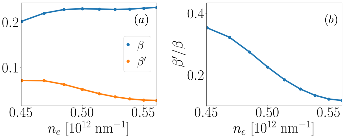
Figure S4: Panel $(a)$ shows the quartic coefficients $\beta$ and $\beta^{\prime}$ as a function of the density $n_{e}$ expressed in arbitrary units. Panel $(b)$ shows the ratio $\beta^{\prime}/\beta$. In this calculation, we employ $k_{B}T=.02$meV, $D=30$meV and the momentum $q_{0}$ is set by the absolute minimum of $K({\bm{q}})$.

C.2 Continuum BdG Hamiltonian of the VAL phase

In this section we derive the microscopic BdG Hamiltonian describing the VAL phase. Starting from the superconducting order parameter $\psi({\bm{r}})=|\psi_{c}|\sum_{j=1}^{3}e^{i{\bm{q}}_{j}\cdot{\bm{r}}}$, the continuum BdG Hamiltonian [28, 29] reads:

$$H_{\rm BdG}=\int d^{2}{\bm{r}}\left[\Psi^{\dagger}\xi_{-i\nabla}\Psi+\frac{1}{4}\Psi^{\dagger}\{\psi({\bm{r}}),-i\bar{\partial}\}\Psi^{\dagger}+h.c.\right],$$ (32)

where $\bar{\partial}=\partial_{x}+i\partial_{y}$ ($-i\bar{\partial}e^{i{\bm{q}}\cdot{\bm{r}}}=e^{i{\bm{q}}\cdot{\bm{r}}}({\bm{q}}_{+}-i\bar{\partial})$), $\{\cdot,\cdot\}$ is the anticommutator.

We now introduce the reciprocal lattice vectors ${\bm{g}}=n_{1}{\bm{g}}_{1}+n_{2}{\bm{g}}_{2}$ where ${\bm{g}}_{1}={\bm{q}}_{1}-{\bm{q}}_{2}$ and ${\bm{g}}_{2}={\bm{q}}_{2}-{\bm{q}}_{3}$ (${\bm{g}}_{3}={\bm{q}}_{3}-{\bm{q}}_{1}$). Given ${\bm{k}}\in\Pi$ in the first Brillouin zone $\Pi$, the BdG Hamiltonian expanded in plane waves reads:

$$\begin{split}H_{\rm BdG}({\bm{k}})&=\frac{1}{2}\sum_{{\bm{g}}}\left[\xi_{{\bm{k}}+{\bm{g}}}c^{\dagger}_{{\bm{k}}+{\bm{g}}}c_{{\bm{k}}+{\bm{g}}}-\xi_{-{\bm{k}}-{\bm{g}}+{\bm{q}}_{1}}c_{-{\bm{k}}-{\bm{g}}+{\bm{q}}_{1}}c^{\dagger}_{-{\bm{k}}-{\bm{g}}+{\bm{q}}_{1}}\right]\\ &+\frac{1}{2}\sum_{j=1}^{3}\psi_{j}\sum_{{\bm{g}}}\left({\bm{k}}+{\bm{g}}-\frac{{\bm{q}}_{j}}{2}\right)_{+}c^{\dagger}_{{\bm{k}}+{\bm{g}}}c^{\dagger}_{{\bm{q}}_{1}-\bm{Q}_{j}-{\bm{g}}-{\bm{k}}}+h.c.,\end{split}$$ (33)

where $\bm{Q}_{j}={\bm{q}}_{1}-{\bm{q}}_{j}$ and ${\bm{k}}_{\pm}=k_{x}\pm ik_{y}$. Using the Nambu basis:

$$\Phi_{{\bm{g}}}({\bm{k}})=\begin{pmatrix}c_{{\bm{k}}+{\bm{g}}}\\ c^{\dagger}_{{\bm{q}}_{1}-{\bm{k}}-{\bm{g}}}\end{pmatrix},$$ (34)

the Hamiltonian takes the compact form:

$$H_{\rm BdG}({\bm{k}})=\frac{1}{2}\sum_{{\bm{g}}}\Phi^{\dagger}_{{\bm{g}}}({\bm{k}})h_{{\bm{g}}{\bm{g}}^{\prime}}({\bm{k}})\Phi_{{\bm{g}}^{\prime}}({\bm{k}}).$$ (35)

In the latter expression we have:

$$h_{{\bm{g}}{\bm{g}}^{\prime}}({\bm{k}})=\delta_{{\bm{g}}{\bm{g}}^{\prime}}\begin{pmatrix}\xi_{{\bm{k}}+{\bm{g}}}&0\\ 0&-\xi_{{\bm{q}}_{1}-{\bm{k}}-{\bm{g}}}\end{pmatrix}+|\psi_{c}|\sum_{j=1}^{3}\delta_{{\bm{g}}^{\prime},{\bm{g}}+\bm{Q}_{j}}\tau^{+}\left({\bm{k}}+{\bm{g}}-\frac{\bm{q}_{j}}{2}\right)_{+}+h.c.,$$ (36)

where $\tau^{\pm}$ are raising and lowering matrices in the Nambu space.

References

- Han et al. [2024] T. Han, Z. Lu, Y. Yao, L. Shi, J. Yang, J. Seo, S. Ye, Z. Wu, M. Zhou, H. Liu, G. Shi, Z. Hua, K. Watanabe, T. Taniguchi, P. Xiong, L. Fu, and L. Ju, Signatures of chiral superconductivity in rhombohedral graphene (2024), arXiv:2408.15233 [cond-mat.mes-hall] .
- Anderson [1959] P. Anderson, Theory of dirty superconductors, Journal of Physics and Chemistry of Solids 11, 26 (1959).
- Kal [2016] Chiral superconductors, Reports on Progress in Physics 79, 054502 (2016).
- Maeno et al. [2024] Y. Maeno, A. Ikeda, and G. Mattoni, Thirty years of puzzling superconductivity in sr2ruo4, Nature Physics 20, 1712 (2024).
- Volovik [1999] G. E. Volovik, Fermion zero modes on vortices in chiral superconductors, Journal of Experimental and Theoretical Physics Letters 70, 609 (1999).
- Read and Green [2000] N. Read and D. Green, Paired states of fermions in two dimensions with breaking of parity and time-reversal symmetries and the fractional quantum hall effect, Phys. Rev. B 61, 10267 (2000).
- Ivanov [2001] D. A. Ivanov, Non-abelian statistics of half-quantum vortices in -wave superconductors, Phys. Rev. Lett. 86, 268 (2001).
- Kozii et al. [2016] V. Kozii, J. W. F. Venderbos, and L. Fu, Three-dimensional majorana fermions in chiral superconductors, Science Advances 2, e1601835 (2016), https://www.science.org/doi/pdf/10.1126/sciadv.1601835 .
- Nayak et al. [2008] C. Nayak, S. H. Simon, A. Stern, M. Freedman, and S. Das Sarma, Non-abelian anyons and topological quantum computation, Rev. Mod. Phys. 80, 1083 (2008).
- Chou et al. [2024] Y.-Z. Chou, J. Zhu, and S. D. Sarma, Intravalley spin-polarized superconductivity in rhombohedral tetralayer graphene (2024), arXiv:2409.06701 [cond-mat.supr-con] .
- Geier et al. [2024] M. Geier, M. Davydova, and L. Fu, Chiral and topological superconductivity in isospin polarized multilayer graphene (2024), arXiv:2409.13829 [cond-mat.supr-con] .
- Yoon et al. [2025] C. Yoon, T. Xu, Y. Barlas, and F. Zhang, Quarter metal superconductivity (2025), arXiv:2502.17555 [cond-mat.mes-hall] .
- Yang and Zhang [2024] H. Yang and Y.-H. Zhang, Topological incommensurate fulde-ferrell-larkin-ovchinnikov superconductor and bogoliubov fermi surface in rhombohedral tetra-layer graphene (2024), arXiv:2411.02503 [cond-mat.supr-con] .
- Qin and Wu [2024] Q. Qin and C. Wu, Chiral finite-momentum superconductivity in the tetralayer graphene (2024), arXiv:2412.07145 [cond-mat.supr-con] .
- Jahin and Lin [2024] A. Jahin and S.-Z. Lin, Enhanced kohn-luttinger topological superconductivity in bands with nontrivial geometry (2024), arXiv:2411.09664 [cond-mat.supr-con] .
- Shavit and Alicea [2024] G. Shavit and J. Alicea, Quantum geometric unconventional superconductivity (2024), arXiv:2411.05071 [cond-mat.supr-con] .
- May-Mann et al. [2025] J. May-Mann, T. Helbig, and T. Devakul, How pairing mechanism dictates topology in valley-polarized superconductors with berry curvature (2025), arXiv:2503.05697 [cond-mat.supr-con] .
- Parra-Martinez et al. [2025] G. Parra-Martinez, A. Jimeno-Pozo, V. T. Phong, H. Sainz-Cruz, D. Kaplan, P. Emanuel, Y. Oreg, P. A. Pantaleon, J. A. Silva-Guillen, and F. Guinea, Band renormalization, quarter metals, and chiral superconductivity in rhombohedral tetralayer graphene (2025), arXiv:2502.19474 [cond-mat.str-el] .
- Zhang and Vishwanath [2025] Y.-H. Zhang and A. Vishwanath, Chiral superconductivity in the flat bands of rhombohedral graphene (2025).
- Koshino and McCann [2009] M. Koshino and E. McCann, Trigonal warping and berry’s phase in abc-stacked multilayer graphene, Phys. Rev. B 80, 165409 (2009).
- Zhang et al. [2010] F. Zhang, B. Sahu, H. Min, and A. H. MacDonald, Band structure of -stacked graphene trilayers, Phys. Rev. B 82, 035409 (2010).
- [22] See Supplementary Material at url … for a detailed discussion of the Ginzburg-Landau free energy, the VAL order parameter, as well as the microscopic calculations of the free energy and the Bogoliubov-de Gennes continuum model.
- Vasyukov et al. [2013] D. Vasyukov, Y. Anahory, L. Embon, D. Halbertal, J. Cuppens, L. Neeman, A. Finkler, Y. Segev, Y. Myasoedov, M. L. Rappaport, M. E. Huber, and E. Zeldov, A scanning superconducting quantum interference device with single electron spin sensitivity, Nature Nanotechnology 8, 639 (2013).
- Uri et al. [2016] A. Uri, A. Y. Meltzer, Y. Anahory, L. Embon, E. O. Lachman, D. Halbertal, N. HR, Y. Myasoedov, M. E. Huber, A. F. Young, and E. Zeldov, Electrically tunable multiterminal squid-on-tip, Nano Letters 16, 6910 (2016).
- Gaggioli et al. [2024] F. Gaggioli, G. Blatter, K. S. Novoselov, and V. B. Geshkenbein, Superconductivity in atomically thin films: Two-dimensional critical state model, Phys. Rev. Res. 6, 023190 (2024).
- Blatter et al. [1994] G. Blatter, M. V. Feigel’man, V. B. Geshkenbein, A. I. Larkin, and V. M. Vinokur, Vortices in high-temperature superconductors, Rev. Mod. Phys. 66, 1125 (1994).
- Stephen and Bardeen [1965] M. J. Stephen and J. Bardeen, Viscosity of type-ii superconductors, Phys. Rev. Lett. 14, 112 (1965).
- Franz and Tešanović [2000] M. Franz and Z. Tešanović, Quasiparticles in the vortex lattice of unconventional superconductors: Bloch waves or landau levels?, Phys. Rev. Lett. 84, 554 (2000).
- Vafek et al. [2001] O. Vafek, A. Melikyan, and Z. Tešanović, Quasiparticle hall transport of d-wave superconductors in the vortex state, Phys. Rev. B 64, 224508 (2001).
- Chiu et al. [2015] C.-K. Chiu, D. I. Pikulin, and M. Franz, Strongly interacting majorana fermions, Phys. Rev. B 91, 165402 (2015).
- Liu and Franz [2015] T. Liu and M. Franz, Electronic structure of topological superconductors in the presence of a vortex lattice, Phys. Rev. B 92, 134519 (2015).
- Pu et al. [2024] S. Pu, J. D. Sau, and R.-X. Zhang, Topologically protected emergent fermi surface in an abrikosov vortex lattice (2024), arXiv:2402.18627 [cond-mat.supr-con] .
- Kraus et al. [2009] Y. E. Kraus, A. Auerbach, H. A. Fertig, and S. H. Simon, Majorana fermions of a two-dimensional superconductor, Phys. Rev. B 79, 134515 (2009).
- Pomeranchuk [1950] I. Y. Pomeranchuk, On the theory of he3, Zh. Eksp. i Teor. Fiz. 20, 919 (1950).
- Rozen et al. [2021] A. Rozen, J. M. Park, U. Zondiner, Y. Cao, D. Rodan-Legrain, T. Taniguchi, K. Watanabe, Y. Oreg, A. Stern, E. Berg, P. Jarillo-Herrero, and S. Ilani, Entropic evidence for a pomeranchuk effect in magic-angle graphene, Nature 592, 214 (2021).
- Saito et al. [2021] Y. Saito, F. Yang, J. Ge, X. Liu, T. Taniguchi, K. Watanabe, J. I. A. Li, E. Berg, and A. F. Young, Isospin pomeranchuk effect in twisted bilayer graphene, Nature 592, 220 (2021).
- Zhang [1993] S.-C. Zhang, Vortex-antivortex lattice in superfluid films, Phys. Rev. Lett. 71, 2142 (1993).
- Gabay and Kapitulnik [1993] M. Gabay and A. Kapitulnik, Vortex-antivortex crystallization in thin superconducting and superfluid films, Phys. Rev. Lett. 71, 2138 (1993).
- Jung and MacDonald [2013] J. Jung and A. H. MacDonald, Gapped broken symmetry states in abc-stacked trilayer graphene, Phys. Rev. B 88, 075408 (2013).
- Dong et al. [2024] J. Dong, T. Wang, T. Wang, T. Soejima, M. P. Zaletel, A. Vishwanath, and D. E. Parker, Anomalous hall crystals in rhombohedral multilayer graphene. i. interaction-driven chern bands and fractional quantum hall states at zero magnetic field, Physical Review Letters 133, 10.1103/physrevlett.133.206503 (2024).
Supplementary materials for: “”
Filippo Gaggioli1, Daniele Guerci1 and Liang Fu1
1Department of Physics, Massachusetts Institute of Technology, Cambridge, MA, USA