Abstract

We study the quantum transport generated by the bipartite entanglement in two-dimensional conformal field theory at finite density with the $U(1)\times U(1)$ symmetry associated to the conservation of the electric charge and of the helicity. The bipartition given by an interval is considered, either on the line or on the circle. The continuity equations and the corresponding conserved quantities for the modular flows of the currents and of the energy-momentum tensor are derived. We investigate the mean values of the associated currents and their quantum fluctuations in the finite density representation, which describe the properties of the modular quantum transport. The modular analogues of the Johnson-Nyquist law and of the fluctuation-dissipation relation are found, which encode the thermal nature of the modular evolution.

Dedicated to the memory of Ivan Todorov

1 Introduction

Entanglement is a fundamental property of quantum systems which can be investigated e.g. by considering a spatial bipartition identified by a subsystem $A$ and its complement $B$. Assuming that the Hilbert space is factorised accordingly and denoting by $\rho$ the state of the entire system, the reduced density matrix $\rho_{A}\equiv\textrm{Tr}_{B}\rho$ obtained by tracing out the degrees of freedom associated to $B$ determines an intrinsic internal dynamics known as modular evolution [1]. This evolution is generated by the modular Hamiltonian $K_{A}$ of the subsystem, which is defined as $\rho_{A}\sim{\rm e}^{-K_{A}}$ and depends on the representation of the theory. A basic feature of the evolution of any quantum system is the existence of conserved charges. Their propagation in spacetime is implemented by the corresponding currents, which generate the quantum transport [2, 3, 4]. In this paper we study the conserved charges, the currents and transport properties associated to the modular evolution.

The modular Hamiltonian is known analytically in very few cases. The most important one corresponds to the theorem of Bisognano and Wichmann [5, 6], which considers the bipartition associated to half space of a local relativistic quantum field theory in its fundamental representation. Another important class of examples is given by conformal field theories (CFT) in two spacetime dimensions, where some modular Hamiltonians $K_{A}$ of an interval $A$ are explicitly known and take a local form in various inequivalent representations [7, 8, 9, 10, 11].

In two-dimensional CFT, besides the fundamental representation, where the quantum transport is rather trivial, other representations at finite particle density and/or finite temperature have been explored [12, 13, 14, 15, 16, 17]. When the left and right moving excitations have different temperature, the underlying states are non-equilibrium steady states (NESS) [18, 19, 20] and display interesting transport properties [13, 14, 15, 16, 21]. Focussing on the zero temperature case for the sake of simplicity, in this paper we study the modular evolution generated by the modular Hamiltonian of an interval $A$ for a CFT in the state characterised by non-vanishing chemical potentials and investigate the corresponding quantum transport.

We consider a local CFT in $1\!+\!1$ spacetime dimensions with $U(1)\times U(1)$ symmetry, implementing the electric charge and the helicity conservation. Along the modular flow, conformal invariance fixes the one-point and two-point functions. In this way one determines the mean values of the currents and their quadratic quantum fluctuations (noise), which provide a physical picture the modular quantum transport in the system.

The paper is organised as follows. In Sec. 2 we discuss the evolution of the basic CFT chiral fields generated by a Hamiltonian depending on a smooth inhomogeneous velocity for each chirality. In Sec. 3 these evolutions are employed to construct currents, continuity equations and conserved quantities in this inhomogeneous CFT. In Sec. 4 we consider the modular evolution for a CFT on the line in the finite density representation and the bipartition determined by an interval is considered and in Sec. 5 the corresponding modular transport properties are investigated. In Sec. 6 and Sec. 7 these analyses are performed for the finite density representation of a CFT at finite volume. Some conclusions are drawn in Sec. 8. Further results and technical details supporting the analyses described in the main text are discussed in the Appendices A, B, C, E, D and F.

2 CFT with spacetime dependent velocities

In this section we focus on some universal algebraic features of CFT in the two-dimensional Minkowski spacetime which hold in any representation.

2.1 Commutation relations

Consider the chiral field algebras $\mathcal{A}_{\pm}=\{T_{\pm}(u),\phi_{\pm}(u),j_{\pm}(u),\dots;\,u\in{\mathbb{R}}\}$ generating the right $(+)$ and left $(-)$ sectors of a CFT with $U(1)$ symmetry. The algebraic properties defining the theory are encoded in commutation relations involving the following chiral field [22, 23, 24, 25]:

(i) the chiral components of the energy-momentum tensor $T_{\pm}$, that satisfy

$$\big{[}\,T_{\pm}(u)\,,T_{\pm}(v)\,\big{]}=\mp\,{\rm i}\,\delta(u-v)\,\partial_{v}T_{\pm}(v)\pm 2{\rm i}\,\delta^{\prime}(u-v)\,T_{\pm}(v)\mp{\rm i}\,\frac{c}{24\pi}\,\delta^{\prime\prime\prime}(u-v)$$ (2.1)

where $c$ is the central charge of the CFT model;

(ii) the complex primary fields $\phi_{\pm}$, with dimensions $h_{\pm}$, occurring into

$$\big{[}\,T_{\pm}(u)\,,\phi_{\pm}(v)\,\big{]} = \mp\,{\rm i}\,\delta(u-v)\,\partial_{v}\phi_{\pm}(v)\pm{\rm i}\,h_{\pm}\,\delta^{\prime}(u-v)\,\phi_{\pm}(v)$$ (2.2)

$$\big{[}\,T_{\pm}(u)\,,\phi^{*}_{\pm}(v)\,\big{]} = \mp\,{\rm i}\,\delta(u-v)\ \partial_{v}\phi^{*}_{\pm}(v)\pm{\rm i}\,h_{\pm}\delta^{\prime}(u-v)\,\phi^{*}_{\pm}(v)$$ (2.3)

which are consistent with (2.1).

(iii) the chiral components of a conserved current $j_{\pm}$, with dimension $h_{j_{\pm}}=1$, which generate the $U(1)$ transformations and satisfy

$$\big{[}\,j_{\pm}(u)\,,\phi_{\pm}(v)\,\big{]}=-\,\delta(u-v)\,\phi_{\pm}(v)\;\;\;\qquad\;\;\;\big{[}\,j_{\pm}(u)\,,\,\phi^{*}_{\pm}(v)\,\big{]}=\delta(u-v)\,\phi^{*}_{\pm}(v)\,.$$ (2.4)

The commutators (2.4) imply that the charge of $\phi$ and $\phi^{*}$ are equal to $-1$ and $1$ respectively. Moreover,

$$\big{[}\,j_{\pm}(u)\,,\,j_{\pm}(v)\,\big{]}=\mp\,{\rm i}\,\frac{\kappa}{2\pi}\,\delta^{\prime}(u-v)$$ (2.5)

where $\kappa$ is a real constant and the r.h.s. is known as Schwinger term.

In the Appendix A we report some consistency checks for the commutators (2.1) and (2.5) through the two-point functions in the fundamental representation which determines the normalization of the two-point functions for $j_{\pm}$ and $T_{\pm}$.

In order to obtain a conventional quantum field theory structure from the above algebraic setting, one should fix a Hilbert space representation $\mathcal{H}_{+}$ and $\mathcal{H}_{-}$ of the chiral algebras $\mathcal{A}_{+}$ and $\mathcal{A}_{-}$ respectively. After smearing with smooth test functions, the elements of $\mathcal{A}_{\pm}$ act as operators in $\mathcal{H}_{+}\otimes\mathcal{H}_{-}$, that represents the physical state space of the system. Before fixing $\mathcal{H}_{\pm}$, in the following we employ (2.1)-(2.5) to obtain some results which are independent of the representation.

2.2 Evolution through spacetime dependent velocities

In the following we consider a general setting where the temporal evolution of the right and the left sectors of the CFT is characterised by two independent velocities $V_{\pm}(u_{\pm})$, which are smooth real functions depending on the light-cone coordinates $u_{\pm}\equiv x\pm t$. In particular, we focus on the Hamiltonian

$$H=\int_{-\infty}^{\infty}\!V_{+}(u_{+})\,{\cal T}_{+}(u_{+})\,{\rm d}u_{+}+\int_{-\infty}^{\infty}\!V_{-}(u_{-})\,{\cal T}_{-}(u_{-})\,{\rm d}u_{-}$$ (2.6)

where

$${\cal T}_{\pm}(u)\equiv T_{\pm}(u)-\mu_{\pm}\,j_{\pm}(u)$$ (2.7)

being $\mu_{\pm}$ defined as the chemical potentials associated to the two chiralities. The temporal evolution generated by (2.6) with $\mu_{+}=\mu_{-}=0$ and $V_{+}=V_{-}$ independent of $t$ has been studied also in [26].

The evolution of the primary fields $\phi_{\pm}(u)$ generated by (2.6) is

$$\phi_{\pm}(\tau,u)\equiv{\rm e}^{{\rm i}\tau H}\,\phi_{\pm}(u)\,{\rm e}^{-{\rm i}\tau H}$$ (2.8)

where $\tau$ will be called modular time to highlight its different role with respect to the physical time $t$. Notice that the dimension of $V_{\pm}$ determines the dimension of $\tau$. Furthermore, we remark that adding a real constant in the r.h.s. of (2.6) does not influence the corresponding evolution (2.8).

Taking the derivative of (2.8) with respect to $\tau$ provides the corresponding equation of motion

$$\partial_{\tau}\phi_{\pm}(\tau,u)\,=\,{\rm i}\,\big{[}\,H,\phi_{\pm}(\tau,u)\,\big{]}\,=\,{\rm i}\,\big{[}\,H\,,{\rm e}^{{\rm i}\tau H}\,\phi_{\pm}(u)\,{\rm e}^{-{\rm i}\tau H}\,\big{]}\,=\,{\rm i}\,{\rm e}^{{\rm i}\tau H}\,\big{[}\,H\,,\phi_{\pm}(u)\,\big{]}\,{\rm e}^{-{\rm i}\tau H}\,.$$ (2.9)

By using (2.2), the first commutator in (2.4) and (2.6), for finite values of $u$ one finds

$$\partial_{\tau}\phi_{\pm}(\tau,u) = {\rm e}^{{\rm i}\tau H}\,\int_{-\infty}^{\infty}\!V_{\pm}(v)\,\Big{\{}\delta(v-u)\,(\pm\,\partial_{u}+{\rm i}\mu_{\pm})\phi_{\pm}(u)\mp h_{\pm}\,\partial_{v}\delta(v-u)\phi_{\pm}(u)\Big{\}}\,{\rm d}v\,{\rm e}^{-{\rm i}\tau H}$$ (2.10)

$$= {\rm e}^{{\rm i}\tau H}\,\Big{\{}\!\pm V_{\pm}(u)\big{(}\partial_{u}\pm{\rm i}\mu_{\pm}\big{)}\phi_{\pm}(u)\pm h_{\pm}\big{[}\partial_{u}V_{\pm}(u)\big{]}\phi_{\pm}(u)\Big{\}}\,{\rm e}^{-{\rm i}\tau H}\qquad\qquad\qquad$$

which leads to

$$\partial_{\tau}\phi_{\pm}(\tau,u)=\pm\,V_{\pm}(u)\big{(}\partial_{u}\pm{\rm i}\mu_{\pm}\big{)}\phi_{\pm}(\tau,u)\pm h_{\pm}\big{[}\partial_{u}V_{\pm}(u)\big{]}\phi_{\pm}(\tau,u)\,.$$ (2.11)

In order to solve (2.11), let us consider the following linear first order equation

$$\partial_{\tau}\xi_{\pm}(\tau,u)=\pm\,V_{\pm}(u)\,\partial_{u}\xi_{\pm}(\tau,u)$$ (2.12)

with initial condition

$$\xi_{\pm}(0,u)=u\,.$$ (2.13)

We assume that $V_{\pm}(u)$ are smooth functions with a finite number of zeros; hence they are finite functions for any finite value of $u$. We introduce $w_{\pm}(u)$ through the following condition

$$w^{\prime}_{\pm}(u)=\frac{1}{V_{\pm}(u)}$$ (2.14)

and consider the interval $A\equiv[a,b]$ identified by two consecutive zeros of $V_{\pm}(u)$, i.e.

$$V_{\pm}(a)=V_{\pm}(b)=0\,.$$ (2.15)

When $u\in A$, the function $w_{\pm}(u)$ is monotonic and therefore its inverse function $w^{-1}_{\pm}(u)$ is well defined. In this case, we define

$$\xi_{\pm}(\tau,u)\equiv w_{\pm}^{-1}\big{(}w_{\pm}(u)\pm\tau\big{)}\,.$$ (2.16)

The functions $\xi_{\pm}(\tau,u)$ satisfy the initial condition (2.13) and

$$\partial_{\tau}\xi_{\pm}(\tau,u)=\pm\,V_{\pm}\big{(}\xi_{\pm}(\tau,u)\big{)}\;\;\;\qquad\;\;\;\partial_{u}\xi_{\pm}(\tau,u)=\frac{V_{\pm}\big{(}\xi_{\pm}(\tau,u)\big{)}}{V_{\pm}(u)}\;.$$ (2.17)

The solution of the equation of motion (2.11) is

$$\phi_{\pm}(\tau,u)\,=\,{\rm e}^{\pm{\rm i}\mu_{\pm}[\xi_{\pm}(\tau,u)-u]}\,\big{[}\partial_{u}\xi_{\pm}(\tau,u)\big{]}^{h_{\pm}}\,\phi_{\pm}\big{(}\xi_{\pm}(\tau,u)\big{)}$$ (2.18)

and satisfies the initial condition

$$\phi_{\pm}(0,u)=\phi_{\pm}(u)\,.$$ (2.19)

Analogously, the evolution of the primary fields $\phi_{\pm}^{*}$ is described by

$$\phi^{*}_{\pm}(\tau,u)\,=\,{\rm e}^{\mp{\rm i}\mu_{\pm}[\xi_{\pm}(\tau,u)-u]}\,\big{[}\partial_{u}\xi_{\pm}(\tau,u)\big{]}^{h_{\pm}}\,\phi^{*}_{\pm}(\xi_{\pm}(\tau,u))\,.$$ (2.20)

The above considerations can be applied to explore also the evolution of the chiral currents generated by (2.6), namely $j_{\pm}(\tau,u)\equiv{\rm e}^{{\rm i}\tau H}\,j_{\pm}(u)\,{\rm e}^{-{\rm i}\tau H}$. The corresponding equation of motion is affected by the Schwinger term in (2.5) and has the form

$$\partial_{\tau}j_{\pm}(\tau,u) = \pm\,V_{\pm}(u)\,\partial_{u}j_{\pm}(\tau,u)\pm\big{[}\partial_{u}V_{\pm}(u)\big{]}j_{\pm}(\tau,u)\pm\frac{\kappa\mu_{\pm}}{2\pi}\,\partial_{u}V_{\pm}(u)$$ (2.21)

$$= \pm\,\partial_{u}\big{[}V_{\pm}(u)\,j_{\pm}(\tau,u)\big{]}\pm\frac{\kappa\mu_{\pm}}{2\pi}\,\partial_{u}V_{\pm}(u)$$ (2.22)

with initial condition $j_{\pm}(0,u)=j_{\pm}(u)$; whose solution is

$$j_{\pm}(\tau,u)=\big{[}\partial_{u}\xi_{\pm}(\tau,u)\big{]}\,j_{\pm}\big{(}\xi_{\pm}(\tau,u)\big{)}-\frac{\kappa\mu_{\pm}}{2\pi}\,\big{[}1-\partial_{u}\xi_{\pm}(\tau,u)\big{]}\,.$$ (2.23)

The continuity equation (2.22) can be written also as

$$\partial_{\tau}j_{\pm}(\tau,u)=\pm\,\partial_{u}\!\left[\,V_{\pm}(u)\left(j_{\pm}(\tau,u)+\frac{\kappa\mu_{\pm}}{2\pi}\right)\right]$$ (2.24)

or, equivalently, as

$$\partial_{\tau}\!\left(j_{\pm}(\tau,u)+\frac{\kappa\mu_{\pm}}{2\pi}\right)=\pm\,\partial_{u}\!\left[\,V_{\pm}(u)\left(j_{\pm}(\tau,u)+\frac{\kappa\mu_{\pm}}{2\pi}\right)\right].$$ (2.25)

In the representations investigated in this manuscript, the mean value of $j_{\pm}(\tau,u)+\tfrac{\kappa\mu_{\pm}}{2\pi}$ vanishes (see (4.1) and (6.1), with the velocities given by (4.7) and (6.9) respectively). The previous observation leads us to realise that (2.22) is equivalent to

$$\partial_{\tau}\!\left(j_{\pm}(\tau,u)+\tilde{\alpha}_{\pm}\frac{\kappa\mu_{\pm}}{2\pi}\right)=\pm\,\partial_{u}\!\left[\,V_{\pm}(u)\left(j_{\pm}(\tau,u)+\alpha_{\pm}\frac{\kappa\mu_{\pm}}{2\pi}\right)\right]\pm\big{(}1-\alpha_{\pm}\big{)}\frac{\kappa\mu_{\pm}}{2\pi}\,\partial_{u}V_{\pm}(u)$$ (2.26)

where $\alpha_{\pm}$ and $\tilde{\alpha}_{\pm}$ are real constants. However, in our analyses we mainly consider the case where $\alpha_{\pm}=\tilde{\alpha}_{\pm}=0$, as discussed in Sec. 3.1.

The evolution of $T_{\pm}(u)$ generated by (2.6), i.e. $T_{\pm}(\tau,u)\equiv{\rm e}^{{\rm i}\tau H}\,T_{\pm}(u)\,{\rm e}^{-{\rm i}\tau H}$, can be explored by employing (2.1), (2.2) and (2.5), which lead to

$$\partial_{\tau}T_{\pm}(\tau,u)=\pm\,V_{\pm}(u)\,\partial_{u}T_{\pm}(\tau,u)\pm 2\big{[}\partial_{u}V_{\pm}(u)\big{]}T_{\pm}(\tau,u)\mp\frac{c}{24\pi}\,\partial^{3}_{u}V_{\pm}(u)\mp\mu_{\pm}V_{\pm}(u)\,\partial_{u}j_{\pm}(\tau,u)$$ (2.29)

where $j_{\pm}(\tau,u)$ is given by (2.23). The occurrence of $j_{\pm}(\tau,u)$ in (2.29) leads us to consider the evolution of ${\cal T}_{\pm}(u)$, namely ${\cal T}_{\pm}(t,x)\equiv{\rm e}^{{\rm i}tH}\,{\cal T}_{\pm}(x)\,{\rm e}^{-{\rm i}tH}$. Indeed, the equation of motion for these fields reads

$$\partial_{\tau}{\cal T}_{\pm}(\tau,u)=\pm\,V_{\pm}(u)\partial_{u}{\cal T}_{\pm}(\tau,u)\pm 2\big{[}\partial_{u}V_{\pm}(u)\big{]}{\cal T}_{\pm}(\tau,u)\mp\frac{\kappa\mu_{\pm}^{2}}{2\pi}\,\partial_{u}V_{\pm}(u)\mp\frac{c}{24\pi}\,\partial^{3}_{u}V_{\pm}(u)$$ (2.30)

with the initial condition ${\cal T}_{\pm}(0,u)={\cal T}_{\pm}(u)$, where only the field ${\cal T}_{\pm}(\tau,u)$ occurs.

Multiplying both sides of (2.30) by $V_{\pm}(u)$, we obtain the following equivalent form

$$\partial_{\tau}\big{[}V_{\pm}(u)\,{\cal T}_{\pm}(\tau,u)\big{]}=\pm\,\partial_{u}\big{[}V_{\pm}(u)^{2}\,{\cal T}_{\pm}(\tau,u)\big{]}\mp\frac{\kappa\mu_{\pm}^{2}}{4\pi}\,\partial_{u}V_{\pm}(u)^{2}\mp\frac{c}{24\pi}\,V_{\pm}(u)\,\partial^{3}_{u}V_{\pm}(u)\,.$$ (2.31)

This differential equation can be arranged as

$$\partial_{\tau}\!\left[\,V_{\pm}(u)\left({\cal T}_{\pm}(\tau,u)-\frac{\kappa\mu_{\pm}^{2}}{4\pi}\right)\right]=\pm\,\partial_{u}\!\left[\,V_{\pm}(u)^{2}\left({\cal T}_{\pm}(\tau,u)-\frac{\kappa\mu_{\pm}^{2}}{4\pi}\right)\right]\mp\frac{c}{24\pi}\,V_{\pm}(u)\,\partial^{3}_{u}V_{\pm}(u)\,.$$ (2.32)

As done in (2.26) for the differential equation for $j_{\pm}(\tau,u)$, (2.32) can be written also in a general form involving the constants $\alpha_{\pm}$ and $\tilde{\alpha}_{\pm}$ that we do not find worth reporting here.

In the finite density representation on the line, where the mean values (4.1) and the velocity $V_{\pm}(u)=V(u)$ in (4.7) must be used, the operators ${\cal T}_{\pm}(\tau,u)-\tfrac{\kappa\mu_{\pm}^{2}}{4\pi}$ have vanishing mean values and $\partial^{3}_{u}V(u)=0$. Instead, in the finite density representation on the circle of length $L$, where the mean values (6.1) and the velocity $V_{\pm}(u)=V_{L}(u)$ in (6.9) must be employed, it is more convenient to write (2.32) as follows

$$\partial_{\tau}\!\left[\,V_{\pm}(u)\left({\cal T}_{\pm}(\tau,u)-\frac{\kappa\mu_{\pm}^{2}}{4\pi}+\frac{\pi c}{12L^{2}}\right)\right] = \pm\,\partial_{u}\!\left[\,V_{\pm}(u)^{2}\left({\cal T}_{\pm}(\tau,u)-\frac{\kappa\mu_{\pm}^{2}}{4\pi}+\frac{\pi c}{12L^{2}}\right)\right]$$

$$\mp\,\frac{c}{24\pi}\left(\frac{2\pi^{2}}{L^{2}}\,\partial_{u}V_{\pm}(u)^{2}+V_{\pm}(u)\,\partial^{3}_{u}V_{\pm}(u)\right).\hskip 31.2982pt$$ (2.33)

Indeed, in this representation the operators within the round brackets in (2.2) have vanishing mean values and $\tfrac{2\pi^{2}}{L^{2}}\,\partial_{u}V_{L}(u)^{2}+V_{L}(u)\,\partial^{3}_{u}V_{L}(u)=0$ for the velocity (6.9).

The solution of (2.30) reads

$${\cal T}_{\pm}(\tau,u)=\big{[}\partial_{u}\xi_{\pm}(\tau,u)\big{]}^{2}\,{\cal T}_{\pm}\big{(}\xi_{\pm}(\tau,u)\big{)}+\frac{\kappa\mu^{2}_{\pm}}{4\pi}\,\Big{\{}1-\big{[}\partial_{u}\xi_{\pm}(\tau,u)\big{]}^{2}\Big{\}}-\frac{c}{24\pi}\,\mathcal{S}_{u}[\xi_{\pm}](\tau,u)$$ (2.34)

where $\mathcal{S}_{u}[\xi](\tau,u)$ is the Schwarzian derivative of the functions $\xi_{\pm}(\tau,u)$, i.e.

$$\mathcal{S}_{u}[\xi](\tau,u)=\frac{\partial^{3}_{u}\xi(\tau,u)}{\partial_{u}\xi(\tau,u)}-\frac{3}{2}\left[\frac{\partial^{2}_{u}\xi(\tau,u)}{\partial_{u}\xi(\tau,u)}\right]^{2}.$$ (2.35)

The solution (2.34) has been found by exploiting the following identity

$$\partial_{\tau}\mathcal{S}_{u}[\xi_{\pm}](\tau,u)=\pm\,V_{\pm}(u)\,\partial_{u}\mathcal{S}_{u}[\xi_{\pm}](\tau,u)\pm 2\big{[}\partial_{u}V_{\pm}(u)\big{]}\mathcal{S}_{u}[\xi_{\pm}](\tau,u)\pm\partial^{3}_{u}V_{\pm}(u)$$ (2.36)

which is a consequence of (2.12) and (2.35). Multiplying (2.36) by $V_{\pm}(u)$, it can be written as

$$\partial_{\tau}\big{\{}V_{\pm}(u)\,\mathcal{S}_{u}[\xi_{\pm}](\tau,u)\big{\}}=\pm\,\partial_{u}\big{\{}V_{\pm}(u)^{2}\,\mathcal{S}_{u}[\xi_{\pm}](\tau,u)\big{\}}\pm V_{\pm}(u)\,\partial^{3}_{u}V_{\pm}(u)\,.$$ (2.37)

By employing the second expression in (2.17), one finds that (2.35) can be expressed as follows

$$\mathcal{S}_{u}[\xi_{\pm}](\tau,u) = \frac{V_{\pm}\big{(}\xi(\tau,u)\big{)}^{2}}{V_{\pm}(u)^{2}}\left[\,\frac{\partial^{2}_{u}V_{\pm}\big{(}\xi(\tau,u)\big{)}}{V_{\pm}\big{(}\xi(\tau,u)\big{)}}-\frac{1}{2}\Bigg{(}\frac{\partial_{u}V_{\pm}\big{(}\xi(\tau,u)\big{)}}{V_{\pm}\big{(}\xi(\tau,u)\big{)}}\Bigg{)}^{2}\,\right]$$

$$-\left[\,\frac{\partial^{2}_{u}V_{\pm}(u)}{V_{\pm}(u)}-\frac{1}{2}\bigg{(}\frac{\partial_{u}V_{\pm}(u)}{V_{\pm}(u)}\bigg{)}^{2}\,\right].$$ (2.38)

This result will be applied in Sec. 4.2 and Sec. 6.2 for specific expressions of $V_{\pm}(u)$.

3 Conservation laws, currents and charges

In this section we discuss the conservation of some charges in the spacetime diamond

$$\mathcal{D}_{A}\equiv\big{\{}(x,t):\,a\leqslant u_{+}\leqslant b\,,\;a\leqslant u_{-}\leqslant b\,\big{\}}$$ (3.1)

corresponding to the domain of dependence of the interval $A\equiv[a,b]$, which can be identified by two consecutive zeros $a<b$ of $V_{\pm}(u)$. The spacetime coordinates $(x,t)$ of the vertices of $\mathcal{D}_{A}$ are $P_{a}=(a,0)$, $P_{b}=(b,0)$, $P_{+\infty}=(\tfrac{a+b}{2},\tfrac{b-a}{2})$ and $P_{-\infty}=(\tfrac{a+b}{2},-\tfrac{b-a}{2})$. The function (2.16) provides $\xi_{\pm}(\tau,u_{\pm})$, which allow to construct the trajectory in $\mathcal{D}_{A}$ parameterised by $\tau\in{\mathbb{R}}$ whose generic point has spacetime coordinates

$$x(\tau)=\frac{\xi_{+}(\tau,u_{+})+\xi_{-}(\tau,u_{-})}{2}\;\;\;\qquad\;\;\;t(\tau)=\frac{\xi_{+}(\tau,u_{+})-\xi_{-}(\tau,u_{-})}{2}$$ (3.2)

where $(u_{+},u_{-})$ are the light-cone coordinates of the initial point corresponding to $\tau=0$.

3.1 Electric charge and helicity

From the commutation relations (2.4), the electric charge density at $\tau=0$ is

$$\varrho(\tau=0;x,t)\equiv j_{+}(u_{+})+j_{-}(u_{-})$$ (3.3)

where $u_{\pm}=x\pm t$ are the light-cone coordinates. Hence, its modular evolution reads

$$\varrho(\tau;x,t)\equiv j_{+}(\tau,u_{+})+j_{-}(\tau,u_{-})$$ (3.4)

where $j_{\pm}(\tau,u_{\pm})$ are given by (2.23).

We remark that the quantity (3.4) and all the subsequent ones defined in a similar way depend both on the physical time $t$ associated to the Hamiltonian of the CFT and on the evolution parameter $\tau$ associated to the Hamiltonian (2.6), which will play the role of the modular Hamiltonian from the next section.

By using (2.21) and $\partial_{x}=\partial_{u_{+}}+\partial_{u_{-}}$, for $\mu_{\pm}=0$ we find the continuity relation

$$\partial_{\tau}\varrho(\tau;x,t)=-\,\partial_{x}j_{x}(\tau;x,t)$$ (3.5)

where

$$j_{x}(\tau;x,t)\equiv-\,V_{+}(u_{+})\,j_{+}(\tau,u_{+})+V_{-}(u_{-})\,j_{-}(\tau,u_{-})$$ (3.6)

defines the space component of the electric current when spacetime dependent velocities $V_{\pm}(u_{\pm})$ occur. In the special case of $V_{+}(u_{+})=V_{-}(u_{-})=1$ identically and for $\tau=0$, from (2.23) we find that the current (3.6) becomes

$$j_{x}(\tau=0;x,t)\big{|}_{V_{+}=V_{-}=1}\,=\,-\,j_{+}(u_{+})+j_{-}(u_{-})$$ (3.7)

i.e. the standard CFT expressions employed e.g. in [13, 15, 14, 16], which has vanishing expectation value in the fundamental representation.

When $\mu_{\pm}\not=0$, the Schwinger term in (2.5) generates an additional contribution with respect to (3.5). In the case we are exploring, given the definition (3.6), by employing (2.21) and $\partial_{t}=\partial_{u_{+}}-\partial_{u_{-}}$ we find the following continuity equation

$$\partial_{\tau}\varrho(\tau;x,t)=-\,\partial_{x}j_{x}(\tau;x,t)+\frac{\kappa}{2\pi}\,\partial_{t}\big{[}\,\mu_{+}\,V_{+}(u_{+})+\mu_{-}\,V_{-}(u_{-})\,\big{]}$$ (3.8)

which naturally leads us to introduce the following $t$-component for the charge current

$$j_{t}(\tau;x,t)\equiv\frac{\kappa}{2\pi}\,\big{[}\,\mu_{+}\,V_{+}(u_{+})+\mu_{-}\,V_{-}(u_{-})\,\big{]}$$ (3.9)

which is independent of $\tau$.

We emphasize that, from either (2.21) or (2.24) and $\partial_{x}=\partial_{u_{+}}+\partial_{u_{-}}$, it is straightforward to observe that (3.8) can be written also as

$$\partial_{\tau}\varrho(\tau;x,t) = -\,\partial_{x}j_{x}(\tau;x,t)+\frac{\kappa}{2\pi}\,\partial_{x}\big{[}\,\mu_{+}\,V_{+}(u_{+})-\mu_{-}\,V_{-}(u_{-})\,\big{]}$$ (3.10)

$$= -\,\partial_{x}\left(j_{x}(\tau;x,t)-\frac{\kappa}{2\pi}\,\big{[}\,\mu_{+}\,V_{+}(u_{+})-\mu_{-}\,V_{-}(u_{-})\,\big{]}\right).$$ (3.11)

This observation, or (2.25), leads us to introduce instead the operators

$$\hat{\varrho}(\tau;x,t)\equiv\left(j_{+}(\tau,u_{+})+\frac{\kappa\mu_{+}}{2\pi}\right)+\left(j_{-}(\tau,u_{-})+\frac{\kappa\mu_{-}}{2\pi}\right)$$ (3.12)

and

$$\hat{j}_{x}(\tau;x,t)\equiv-\,V_{+}(u_{+})\left(j_{+}(\tau,u_{+})+\frac{\kappa\mu_{+}}{2\pi}\right)+V_{-}(u_{-})\left(j_{-}(\tau,u_{-})+\frac{\kappa\mu_{-}}{2\pi}\right)$$ (3.13)

which satisfy the following continuity equation also when $\mu_{\pm}\neq 0$

$$\partial_{\tau}\hat{\varrho}(\tau;x,t)=-\,\partial_{x}\hat{j}_{x}(\tau;x,t)\,.$$ (3.14)

In Sec. 4.1 we will see that the operators (3.12) and (3.13) have vanishing mean values in the finite density representation; hence they do not provide the operators employed in [13, 15, 14, 16] when $\tau=0$ and $V_{+}(u_{+})=V_{-}(u_{-})=1$ identically. Thus, in our analysis we mainly adopt the definitions (3.4) and (3.6).

In the following, also for the helicity, the energy and the momentum we can introduce operators having vanishing mean values in the finite density representation and playing the same role of (3.12) and (3.13). The above considerations are straightforwardly adapted to these operators.

By employing (3.9), the continuity relation (3.8) takes the form

$$\partial_{\tau}\varrho(\tau;x,t)=-\,\partial_{x}j_{x}(\tau;x,t)+\partial_{t}j_{t}(\tau;x,t)$$ (3.15)

which can be rewritten also in following covariant form

$$\partial_{\tau}\varrho(\tau;x,t)=\partial_{\mu}j^{\mu}(\tau;x,t)$$ (3.16)

via the Minkowski metric $\eta_{\mu\nu}\equiv\textrm{diag}(1,-1)$ in the spacetime parameterised by $x^{\mu}=(t,x)$, that allows to raise the index of the vector $j_{\mu}\equiv(j_{t},j_{x})$, finding $j^{\mu}\equiv(j_{t},\,-j_{x})$.

We remark that the arbitrary additive constant shifts in (3.6) and (3.9) can be fixed also by requiring the vanishing of these quantities at the vertices $P_{a}$, $P_{b}$, $P_{+\infty}$ and $P_{-\infty}$ of the spacetime diamond $\mathcal{D}_{A}$ in (3.1), i.e. for $u_{\pm}\in\{a,b\}$.

From (3.4), we can define the total electric charge in $\mathcal{D}_{A}$ as

$$Q_{A}\equiv\int_{\mathcal{D}_{A}}\!\!\varrho(\tau;x,t)\,{\rm d}x\,{\rm d}t\,=\,\frac{b-a}{2}\left(\,\int_{a}^{b}j_{+}(\tau,u_{+})\,{\rm d}u_{+}+\int_{a}^{b}j_{-}(\tau,u_{-})\,{\rm d}u_{-}\right)$$ (3.17)

which is independent of $x$ and $t$ by construction. The independence of $\tau$ in (3.17), i.e. the condition $\partial_{\tau}Q_{A}=0$ corresponding to the conservation of $Q_{A}$ in $\mathcal{D}_{A}$, follows from the equations of motion for the currents in (2.21) combined with (2.15).

From (3.6) and (3.9), notice that $\partial_{\tau}j_{x}$ is non vanishing, while $\partial_{\tau}j_{t}=0$, being $j_{t}$ independent of $\tau$. In particular, by employing (2.22) we obtain

$$\partial_{\tau}j_{x}(\tau;x,t) = -\,\partial_{u_{+}}\!\big{[}\,V_{+}(u_{+})^{2}\,j_{+}(\tau,u_{+})\,\big{]}-\partial_{u_{-}}\!\big{[}\,V_{-}(u_{-})^{2}\,j_{+}(\tau,u_{-})\,\big{]}$$

$$+\,\frac{\partial_{u_{+}}\!V_{+}(u_{+})^{2}}{2}\;j_{+}(\tau,u_{+})+\frac{\partial_{u_{-}}\!V_{-}(u_{-})^{2}}{2}\;j_{-}(\tau,u_{-})$$ (3.18)

$$-\;\frac{\kappa}{4\pi}\Big{[}\,\mu_{+}\,\partial_{u_{+}}\!V_{+}(u_{+})^{2}+\mu_{-}\,\partial_{u_{-}}\!V_{-}(u_{-})^{2}\,\Big{]}$$

which implies that $j_{x}(\tau;x,t)$ does not correspond to the density of a conserved quantity in the diamond $\mathcal{D}_{A}$. This happens because of the terms in the second line of (3.1); indeed the first line and the third line can be written as total derivatives e.g. in $x$ and $t$ respectively.

The helicity can be investigated in a similar way. Since $\phi_{+}$ and $\phi_{-}$ have opposite helicities, the commutators (2.4) lead us to introduce the following density

$$\chi(\tau;x,t)\equiv j_{+}(\tau,u_{+})-j_{-}(\tau,u_{-})\,.$$ (3.19)

From (2.21), we find the continuity relation

$$\partial_{\tau}\chi(\tau;x,t)=\partial_{t}k_{t}(\tau;x,t)-\,\partial_{x}k_{x}(\tau;x,t)=\partial_{\mu}k^{\mu}(\tau;x,t)$$ (3.20)

where the components of the helicity current are defined as

$$k_{x}(\tau;x,t) \equiv -\,V_{+}(u_{+})\,j_{+}(\tau,u_{+})-V_{-}(u_{-})\,j_{-}(\tau,u_{-})$$ (3.21)

$$\rule{0.0pt}{17.07182pt}k_{t}(\tau;x,t) \equiv \frac{\kappa}{2\pi}\,\big{[}\,\mu_{+}\,V_{+}(u_{+})-\mu_{-}\,V_{-}(u_{-})\,\big{]}$$ (3.22)

which vanish for $u_{\pm}\in\{a,b\}$. The helicity charge in $\mathcal{D}_{A}$ following from (3.19) is

$$\widetilde{Q}_{A}\equiv\int_{\mathcal{D}_{A}}\!\!\chi(\tau;x,t)\,{\rm d}x\,{\rm d}t\,=\,\frac{b-a}{2}\left(\,\int_{a}^{b}j_{+}(\tau,u_{+})\,{\rm d}u_{+}-\int_{a}^{b}j_{-}(\tau,u_{-})\,{\rm d}u_{-}\right).$$ (3.23)

This quantity is independent of $x$, $t$ and also conserved, i.e. independent of $\tau$, as we can find from (2.21) and (2.15).

3.2 Energy and momentum

The energy density can be introduced from (2.6) as follows

$$\mathcal{E}(\tau;x,t)\equiv V_{+}(u_{+})\,{\cal T}_{+}(\tau,u_{+})+V_{-}(u_{-})\,{\cal T}_{-}(\tau,u_{-})+f_{+}(u_{+})+f_{-}(u_{-})$$ (3.24)

and $f_{\pm}(u_{\pm})$ are real functions that can be exploited to fix the mean value of this operator but they do not influence the following analysis because they are independent of $\tau$.

The equations of motion (2.30) lead to

$$\partial_{\tau}\mathcal{E}(\tau;x,t) = \partial_{u_{+}}\big{[}\,V_{+}(u_{+})^{2}\,{\cal T}_{+}(\tau,u_{+})\,\big{]}-\frac{\kappa\,\mu_{+}^{2}}{2\pi}\,\partial_{u_{+}}\big{[}V_{+}(u_{+})^{2}\big{]}-\frac{c}{24\pi}\,V_{+}(u_{+})\,\partial_{u_{+}}^{3}V_{+}(u_{+})$$

$$-\,\partial_{u_{-}}\big{[}\,V_{-}(u_{-})^{2}\,{\cal T}_{-}(\tau,u_{-})\,\big{]}+\frac{\kappa\,\mu_{-}^{2}}{2\pi}\,\partial_{u_{-}}\big{[}V_{-}(u_{-})^{2}\big{]}+\frac{c}{24\pi}\,V_{-}(u_{-})\,\partial_{u_{-}}^{3}V_{-}(u_{-})\,.$$

By using the following identity

$$\partial_{u}\big{(}V(u)^{2}\,\mathcal{V}[V](u)\big{)}=\,V(u)\,\partial_{u}^{3}V(u)$$ (3.26)

where

$$\mathcal{V}[V](u)\equiv\frac{V^{\prime\prime}(u)}{V(u)}-\frac{1}{2}\left[\frac{V^{\prime}(u)}{V(u)}\right]^{2}$$ (3.27)

and the fact that $\partial_{x}=\partial_{u_{+}}+\partial_{u_{-}}$ and $\partial_{t}=\partial_{u_{+}}-\partial_{u_{-}}$, the differential equation (3.2) can be written also in the form of the continuity relation

$$\partial_{\tau}\mathcal{E}(\tau;x,t)=\partial_{t}\mathcal{J}_{t}(\tau;x,t)-\partial_{x}\mathcal{J}_{x}(\tau;x,t)=\partial_{\mu}\mathcal{J}^{\mu}(\tau;x,t)$$ (3.28)

where

$$\mathcal{J}_{x}(\tau;x,t) \equiv -\,V_{+}(u_{+})^{2}\,{\cal T}_{+}(\tau,u_{+})+V_{-}(u_{-})^{2}\,{\cal T}_{-}(\tau,u_{-})$$ (3.29)

$$\rule{0.0pt}{22.76228pt}\rule{0.0pt}{19.91684pt}\mathcal{J}_{t}(\tau;x,t) \equiv -\,\frac{\kappa}{4\pi}\,\Big{\{}\mu^{2}_{+}\,V_{+}(u_{+})^{2}+\mu^{2}_{-}\,V_{-}(u_{-})^{2}\Big{\}}$$

$$-\,\frac{c}{24\pi}\,\Big{\{}V_{+}(u_{+})^{2}\,\mathcal{V}[V_{+}](u_{+})+V_{-}(u_{-})^{2}\,\mathcal{V}[V_{-}](u_{-})\Big{\}}+C_{\mathcal{J}}\,.$$ (3.30)

We remark that (3.29) satisfies

$$\mathcal{J}_{x}(\tau=0;x,t)\big{|}_{V_{+}=V_{-}=1}=-\,{\cal T}_{+}(u_{+})+{\cal T}_{-}(u_{-})$$ (3.31)

whose expectation value in the finite density representation (see (4.1)) agrees with the corresponding result found in [15] at zero temperature. In (3.2) we have introduced the constant $C_{\mathcal{J}}$ because, while $\mathcal{J}_{x}$ vanishes for $u_{\pm}\in\{a,b\}$, this condition is not guaranteed for $\mathcal{J}_{t}$.

The energy density (3.24) leads us to define the total energy in $\mathcal{D}_{A}$ as follows

$$E_{A} \equiv \int_{\mathcal{D}_{A}}\!\!\mathcal{E}(\tau;x,t)\,{\rm d}x\,{\rm d}t$$ (3.32)

$$= \frac{b-a}{2}\left(\,\int_{a}^{b}\!\Big{[}V_{+}(u_{+})\,{\cal T}_{+}(\tau,u_{+})+f_{+}(u_{+})\Big{]}{\rm d}u_{+}+\int_{a}^{b}\!\Big{[}V_{-}(u_{-})\,{\cal T}_{-}(\tau,u_{-})+f_{-}(u_{-})\Big{]}{\rm d}u_{-}\right)$$

which is constant, i.e. independent of $x$, $t$ and $\tau$. Its conservation along the $\tau$-evolution, i.e. the fact that $\partial_{\tau}E_{A}=0$, is obtained from the continuity equation (3.2), the identity (3.26) and the condition (2.15).

By employing (2.31), from (3.2) and (3.29) we obtain respectively $\partial_{\tau}\mathcal{J}_{t}=0$ and

$$\partial_{\tau}\mathcal{J}_{x}(\tau;x,t) = -\,\partial_{u_{+}}\!\big{[}\,V_{+}(u_{+})^{3}\,\mathcal{T}_{+}(\tau,u_{+})\,\big{]}-\partial_{u_{-}}\!\big{[}\,V_{-}(u_{-})^{3}\,\mathcal{T}_{+}(\tau,u_{-})\,\big{]}$$ (3.33)

$$+\,\frac{\partial_{u_{+}}\!V_{+}(u_{+})^{3}}{3}\;\mathcal{T}_{+}(\tau,u_{+})+\frac{\partial_{u_{-}}\!V_{-}(u_{-})^{3}}{3}\;\mathcal{T}_{-}(\tau,u_{-})$$

$$\hskip-73.97733pt+\,\frac{\kappa}{6\pi}\Big{[}\,\mu_{+}^{2}\,\partial_{u_{+}}\!V_{+}(u_{+})^{3}+\mu_{-}^{2}\,\partial_{u_{-}}\!V_{-}(u_{-})^{3}\,\Big{]}+\frac{c}{24\pi}\Big{[}\,V_{+}(u_{+})^{2}\,\partial_{u_{+}}^{3}\!V_{+}(u_{+})+V_{-}(u_{-})^{2}\,\partial_{u_{-}}^{3}\!V_{-}(u_{-})\,\Big{]}$$

which tells us that $\mathcal{J}_{x}(\tau;x,t)$ is not the density of a conserved quantity in the diamond.

We find it worth introducing also the following generalized momentum density

$$\widetilde{\mathcal{E}}(\tau;x,t)\equiv V_{+}(u_{+})\,{\cal T}_{+}(\tau,u_{+})-V_{-}(u_{-})\,{\cal T}_{-}(\tau,u_{-})+f_{+}(u_{+})-f_{-}(u_{-})$$ (3.34)

where for the real functions $f_{\pm}(u_{\pm})$ we can repeat the considerations made below (3.24). The equations of motion (2.30) give

$$\partial_{\tau}\widetilde{\mathcal{E}}(\tau;x,t) = \partial_{u_{+}}\big{[}\,V_{+}(u_{+})^{2}\,{\cal T}_{+}(\tau,u_{+})\,\big{]}-\frac{\kappa\mu_{+}^{2}}{2\pi}\,\partial_{u_{+}}\big{[}V_{+}(u_{+})^{2}\big{]}-\frac{c}{24\pi}\,V_{+}(u_{+})\,\partial_{u_{+}}^{3}V_{+}(u_{+})$$

$$+\,\partial_{u_{-}}\big{[}\,V_{-}(u_{-})^{2}\,{\cal T}_{-}(\tau,u_{-})\,\big{]}-\frac{\kappa\mu_{-}^{2}}{2\pi}\,\partial_{u_{-}}\big{[}V_{-}(u_{-})^{2}\big{]}-\frac{c}{24\pi}\,V_{-}(u_{-})\,\partial_{u_{-}}^{3}V_{-}(u_{-})$$

or, equivalently,

$$\partial_{\tau}\widetilde{\mathcal{E}}(\tau;x,t)=\partial_{t}\widetilde{\mathcal{J}}_{t}(\tau;x,t)-\partial_{x}\widetilde{\mathcal{J}}_{x}(\tau;x,t)=\partial_{\mu}\widetilde{\mathcal{J}}^{\mu}(\tau;x,t)$$ (3.36)

where

$$\widetilde{\mathcal{J}}_{x}(\tau;x,t) \equiv -\,V_{+}(u_{+})^{2}\,{\cal T}_{+}(\tau,u_{+})-V_{-}(u_{-})^{2}\,{\cal T}_{-}(\tau,u_{-})$$ (3.37)

$$\rule{0.0pt}{22.76228pt}\rule{0.0pt}{19.91684pt}\widetilde{\mathcal{J}}_{t}(\tau;x,t) \equiv -\,\frac{\kappa}{4\pi}\,\Big{\{}\mu^{2}_{+}\,V_{+}(u_{+})^{2}-\mu^{2}_{-}\,V_{-}(u_{-})^{2}\Big{\}}$$

$$-\,\frac{c}{24\pi}\,\Big{\{}V_{+}(u_{+})^{2}\,\mathcal{V}[V_{+}](u_{+})-V_{-}(u_{-})^{2}\,\mathcal{V}[V_{-}](u_{-})\Big{\}}+C_{\widetilde{\mathcal{J}}}\,.$$ (3.38)

In analogy with (3.32), the momentum density (3.34) leads us to introduce the total momentum in $\mathcal{D}_{A}$ as follows

$$\widetilde{E}_{A} \equiv \int_{\mathcal{D}_{A}}\!\!\widetilde{\mathcal{E}}(\tau;x,t)\,{\rm d}x\,{\rm d}t$$ (3.39)

$$= \frac{b-a}{2}\left(\,\int_{a}^{b}\!\Big{[}V_{+}(u_{+})\,{\cal T}_{+}(\tau,u_{+})+f_{+}(u_{+})\Big{]}{\rm d}u_{+}-\int_{a}^{b}\!\Big{[}V_{-}(u_{-})\,{\cal T}_{-}(\tau,u_{-})+f_{-}(u_{-})\Big{]}{\rm d}u_{-}\right)$$

which is independent of $x$, $t$ and also of $\tau$, as it can be found from the corresponding continuity equation (3.2), the identity (3.26) and the condition (2.15).

The application of the above analysis to the chiral primaries is discussed in the Appendix B.

3.3 Transformation generated by the generalized momentum

The operator (3.34) provides the following evolution operator

$$P\equiv\int_{-\infty}^{\infty}\!\Big{[}V_{+}(u_{+})\,{\cal T}_{+}(\tau,u_{+})+f_{+}(u_{+})\Big{]}{\rm d}u_{+}-\int_{-\infty}^{\infty}\!\Big{[}V_{-}(u_{-})\,{\cal T}_{-}(\tau,u_{-})+f_{-}(u_{-})\Big{]}{\rm d}u_{-}\,.$$ (3.40)

The evolution of a primary $\phi_{\pm}$ generated by (3.40) reads

$$\widetilde{\phi}_{\pm}(\lambda,u)\equiv{\rm e}^{{\rm i}\lambda P}\,\phi_{\pm}(u)\,{\rm e}^{-{\rm i}\lambda P}$$ (3.41)

and it can be studied by slightly modifying the analysis described for (2.8). This leads to the following equation for (3.41)

$$\partial_{\lambda}\widetilde{\phi}_{\pm}(\lambda,u)=V_{\pm}(u)\big{(}\partial_{u}\pm{\rm i}\mu_{\pm}\big{)}\widetilde{\phi}_{\pm}(\lambda,u)+h_{\pm}\big{[}\partial_{u}V_{\pm}(u)\big{]}\widetilde{\phi}_{\pm}(\lambda,u)$$ (3.42)

with initial condition $\widetilde{\phi}_{\pm}(0,u)=\phi_{\pm}(u)$, which can be solved through $\zeta_{\pm}(\lambda,x)$ satisfying

$$\partial_{\lambda}\zeta_{\pm}(\lambda,u)=V_{\pm}(u)\,\partial_{u}\zeta_{\pm}(\lambda,u)$$ (3.43)

with the initial condition

$$\zeta_{\pm}(0,u)=u\,.$$ (3.44)

which can be compared with the differential equation (2.12) and its initial condition (2.13) respectively. The solution of (3.43) and (3.44) can expressed for $u\in[a,b]$ between two consecutive zeros of $V_{\pm}$ in terms of (2.14) as follows

$$\zeta_{\pm}(\lambda,u)\equiv w_{\pm}^{-1}\big{(}w_{\pm}(u)+\lambda\big{)}$$ (3.45)

which is slightly different from (2.16). The expressions (3.45) satisfy

$$\partial_{\lambda}\zeta_{\pm}(\lambda,u)=V_{\pm}(\zeta_{\pm}(\lambda,u))\;\;\;\qquad\;\;\;\partial_{u}\zeta_{\pm}(\lambda,u)=\frac{V_{\pm}(\zeta_{\pm}(\lambda,u))}{V_{\pm}(u)}\;.$$ (3.46)

Comparing the functions in (3.45) with the ones in (2.16), we observe that $\zeta_{+}(\lambda,u)=\xi_{+}(\lambda,u)$, while $\zeta_{-}(\lambda,u)=\xi_{-}(-\lambda,u)$. The infinitesimal transformation is obtained by expanding (3.45) for small $\lambda$ and this gives (see also the remark 4.2 of [26])

$$\zeta_{\pm}(\lambda,u)=u+V_{\pm}(u)\,\lambda+O(\lambda^{2})\,.$$ (3.47)

For constant velocities $V_{\pm}$, we have $\zeta_{\pm}(\lambda,u)=u+V_{\pm}\lambda$ for (3.45), i.e. the spatial translations.

By using (3.45), for the evolution (3.41) we find

$$\widetilde{\phi}_{\pm}(\lambda,u)={\rm e}^{\pm{\rm i}\mu_{\pm}[\zeta_{\pm}(\lambda,u)-u]}\,\big{[}\partial_{u}\zeta_{\pm}(\lambda,u)\big{]}^{h_{\pm}}\,\phi_{\pm}\big{(}\zeta_{\pm}(\lambda,u)\big{)}$$ (3.48)

which satisfies the initial condition $\widetilde{\phi}_{\pm}(0,u)=\phi_{\pm}(u)$, as expected. Notice that the r.h.s.’s of (2.18) and (3.48) are formally identical. Thus, as for the evolutions in $\lambda$ of $j_{\pm}$ and of ${\cal T}_{\pm}$, i.e.

$$\widetilde{j}_{\pm}(\lambda,u)\equiv{\rm e}^{{\rm i}\lambda\widetilde{H}}\,j_{\pm}(u)\,{\rm e}^{-{\rm i}\lambda\widetilde{H}}\;\;\qquad\;\;\widetilde{{\cal T}}_{\pm}(\lambda,u)\equiv{\rm e}^{{\rm i}\lambda\widetilde{H}}\,{\cal T}_{\pm}(u)\,{\rm e}^{-{\rm i}\lambda\widetilde{H}}$$ (3.49)

we find that they are given by the r.h.s.’s of (2.23) and (2.34) respectively, with $\xi_{\pm}(\tau,u)$ replaced by $\zeta_{\pm}(\lambda,u)$.

Finally, from (3.45) one introduces the trajectories in $\mathcal{D}_{A}$ generated through the evolution governed by (3.40), as done in (3.2) for (2.16), whose spacetime coordinates read

$$x(\lambda)=\frac{\zeta_{+}(\lambda,u_{+})+\zeta_{-}(\lambda,u_{-})}{2}\;\;\;\qquad\;\;\;t(\lambda)=\frac{\zeta_{+}(\lambda,u_{+})-\zeta_{-}(\lambda,u_{-})}{2}$$ (3.50)

where $\lambda\in{\mathbb{R}}$ and $(u_{+},u_{-})$ are the light-cone coordinates of the point corresponding to $\lambda=0$.

3.4 Heat

Any linear combinations of the above conserved currents defines a conserved current as well. From non-equilibrium thermodynamics [27], it is known that the heat density in the system is described by

$$\mathcal{M}(\tau;x,t)=\mathcal{E}(\tau;x,t)-\mu_{c}\,\varrho(\tau;x,t)-\mu_{h}\,\chi(\tau;x,t)$$ (3.51)

defined through (3.4), (3.19) and (3.24), where the electric charge and helicity chemical potentials are the combinations

$$\mu_{e}\equiv\mu_{+}+\mu_{-}\;\;\;\qquad\;\;\;\mu_{h}\equiv\mu_{+}-\mu_{-}\,.$$ (3.52)

Accordingly, the heat flow in the system is generated by the currents

$$q_{x}(\tau;x,t) = \mathcal{J}_{x}(\tau;x,t)-\mu_{e}\,j_{x}(\tau;x,t)-\mu_{h}\,k_{x}(\tau;x,t)$$ (3.53)

$$q_{t}(\tau;x,t) = \,\mathcal{J}_{t}(\tau;x,t)-\mu_{e}\,j_{t}(\tau;x,t)-\mu_{h}\,k_{t}(\tau;x,t)\,.$$ (3.54)

Combining (3.51) with (3.17), (3.23) and (3.32), for the total heat in the diamond $\mathcal{D}_{A}$ we have

$$\mathcal{M}_{A}=E_{A}-\mu_{e}\,Q_{A}-\mu_{h}\,{\widetilde{Q}}_{A}$$ (3.55)

which is independent of $x$, $t$ and $\tau$.

4 Infinite volume

In this section we consider the finite density representation of the CFT on the line, which is characterised by the mean values reported in Sec. 4.1, and the modular Hamiltonian corresponding to the bipartition provided by an interval. The results of Sec. 2.2 are employed to discuss the modular evolution of the fields (Sec. 4.2), the modular conjugation and its geometric action (Sec. 4.3). The modular correlators are considered in Sec. 4.4.

4.1 Finite density representation on the line

In the finite density representation of the CFT on the line, the mean values of the basic chiral fields described in Sec. 2.1 are

$$\langle\phi_{\pm}(u)\rangle_{\mu_{\pm}}=0\;\;\qquad\;\;\langle j_{\pm}(u)\rangle_{\mu_{\pm}}=-\frac{\kappa\mu_{\pm}}{2\pi}\;\;\qquad\;\;\langle{\cal T}_{\pm}(u)\rangle_{\mu_{\pm}}=\frac{\kappa\mu^{2}_{\pm}}{4\pi}\,.$$ (4.1)

These expressions are obtained from the corresponding ones in the fundamental (ground state) representation $\pi_{0}$, where all these one-point function vanish (see the Appendix A) through an automorphism $\gamma_{\mu}=\gamma_{\mu_{+}}\otimes\gamma_{\mu_{-}}$, as discussed in the Appendix C. This automorphism provides the state $\Omega_{\mu_{\pm}}$ from the ground state $\Omega_{0}$, which corresponds to $\mu_{\pm}=0$. The finite density representation is given by $\pi_{0}\circ\gamma_{\mu}$. In the following we denote $\pi_{0}\circ\gamma_{\mu}[\mathcal{O}_{\pm}]$ just by $\mathcal{O}_{\pm}$, with a slight abuse of notation.

This procedure can be employed to find also the two-point functions of these fields in the finite density representation listed below, that are obtained from the ones in the fundamental representation, as explained in the Appendix C). The two-point functions of $\phi_{\pm}$ are (see e.g. [28] for $\mu_{\pm}=0$)

$$\langle\phi_{\pm}^{*}(u)\,\phi_{\pm}(v)\rangle_{\mu_{\pm}}^{\textrm{\tiny con}}=\frac{{\rm e}^{\mp{\rm i}\pi h_{\pm}}\,{\rm e}^{\pm{\rm i}\mu_{\pm}(u-v)}}{2\pi\,(u-v\mp{\rm i}\varepsilon)^{2h_{\pm}}}\;\;\;\qquad\;\;\;\langle\phi_{\pm}(u)\,\phi^{*}_{\pm}(v)\rangle_{\mu_{\pm}}^{\textrm{\tiny con}}=\frac{{\rm e}^{\mp{\rm i}\pi h_{\pm}}\,{\rm e}^{\mp{\rm i}\mu_{\pm}(u-v)}}{2\pi\,(u-v\mp{\rm i}\varepsilon)^{2h_{\pm}}}\,.$$ (4.2)

The two-point functions of $j_{\pm}$ contain the constant $\kappa$ and read

$$\langle j_{\pm}(u)\,j_{\pm}(v)\rangle_{\mu_{\pm}}^{\textrm{\tiny con}}=\frac{\kappa}{4\pi^{2}}\,\frac{1}{(u-v\mp{\rm i}\varepsilon)^{2}}$$ (4.3)

while the two-point functions of ${\cal T}_{\pm}$ depend on the central charge $c$ as follows

$$\langle{\cal T}_{\pm}(u)\,{\cal T}_{\pm}(v)\rangle_{\mu_{\pm}}^{\textrm{\tiny con}}=\frac{c}{8\pi^{2}}\,\frac{1}{(u-v\mp{\rm i}\varepsilon)^{4}}\,.$$ (4.4)

The positivity of (4.2)-(4.4) imply $h_{\pm}\geqslant 0$ (see the Appendix D), $\kappa\geqslant 0$ and $c\geqslant 0$ respectively. Furthermore, we have that

$$\langle{\cal T}_{\pm}(u)\,j_{\pm}(v)\rangle_{\mu_{\pm}}^{\textrm{\tiny con}}=-\,\mu_{\pm}\,\langle j_{\pm}(u)\,j_{\pm}(v)\rangle_{\mu_{\pm}}^{\textrm{\tiny con}}\,.$$ (4.5)

The connected mixed correlators involving fields having different chiralities vanish identically.

When $t\pm x$ are chosen as light-cone coordinates, the $\mp{\rm i}\varepsilon$ must be replaced with $-{\rm i}\varepsilon$ in all the chiral two-point functions occurring in this manuscript.

4.2 Modular Hamiltonian

The results discussed in Sec. 2.2 can be employed to investigate some modular Hamiltonians in two-dimensional CFT corresponding to the spatial bipartition provided by an interval [7, 8, 9, 10].

In the following we consider a CFT on a line and in the finite density state characterised by the correlators reported in Sec. 4.1. The spatial bipartition of the line is given by the interval $A=[a,b]$ and its complement $B=(-\infty,a)\cup(b,+\infty)$. In this setup, the modular Hamiltonian of the interval $A$ reads [9, 11]

$$K_{A}=\int_{A}V(u_{+})\left[\,{\cal T}_{+}(u_{+})-\frac{\kappa\mu^{2}_{+}}{4\pi}\,\right]{\rm d}u_{+}+\int_{A}V(u_{-})\left[\,{\cal T}_{-}(u_{-})-\frac{\kappa\mu^{2}_{-}}{4\pi}\,\right]{\rm d}u_{-}$$ (4.6)

in terms of the chiral operators (2.7), with

$$V(u)=2\pi\,\frac{(b-u)(u-a)}{b-a}=\frac{1}{w^{\prime}(u)}\;\;\;\qquad\;\;\;u\in A$$ (4.7)

where

$$w(u)\equiv\frac{1}{2\pi}\,\log\!\left(\!-\frac{u-a}{u-b}\right).$$ (4.8)

The modular Hamiltonian (4.6) can be obtained by applying the automorphism $\gamma_{\mu}^{-1}$ described in the Appendix C to the corresponding modular Hamiltonian in the fundamental representation (see (C.9)). Notice that the integrand in (4.6) corresponds to the special case of (3.24) where $V_{\pm}(u_{\pm})=V(u_{\pm})$ and $f_{\pm}(u_{\pm})=-\tfrac{\kappa\mu^{2}_{\pm}}{4\pi}V(u_{\pm})$.

The modular Hamiltonian of the complement $B$ can be found by exchanging $a$ and $b$ in (4.7) and (4.8) (in the latter equation also the global sign in the argument of the logarithm must be inverted in order to have a well defined function); hence $V$ changes its global sign. Notice that $-V(u)\geqslant 0$ when $u\in B$. This leads to

$$K_{B}=\int_{B}\big{(}\!-V(u_{+})\big{)}\left[\,{\cal T}_{+}(u_{+})-\frac{\kappa\mu^{2}_{+}}{4\pi}\,\right]{\rm d}u_{+}+\int_{B}\big{(}\!-V(u_{-})\big{)}\left[\,{\cal T}_{-}(u_{-})-\frac{\kappa\mu^{2}_{-}}{4\pi}\,\right]{\rm d}u_{-}\,.$$ (4.9)

We remark that the weight functions in (4.6) and (4.9), which are given by $V(u)$ and $-V(u)$ respectively, are positive in the corresponding domains. The modular Hamiltonians (4.6) and (4.9) provide the full modular Hamiltonian for the bipartition and the finite density state $\Omega_{\mu_{\pm}}$ that we are considering, which reads

$$K \equiv K_{A}\otimes\boldsymbol{1}_{B}-\boldsymbol{1}_{A}\otimes K_{B}$$ (4.10)

$$= \int_{-\infty}^{\infty}V(u_{+})\left[\,{\cal T}_{+}(u_{+})-\frac{\kappa\mu^{2}_{+}}{4\pi}\,\right]{\rm d}u_{+}+\int_{-\infty}^{\infty}V(u_{-})\left[\,{\cal T}_{-}(u_{-})-\frac{\kappa\mu^{2}_{-}}{4\pi}\,\right]{\rm d}u_{-}\,.$$

We remark that, because of the choice $f_{\pm}(u_{\pm})=-\tfrac{\kappa\mu^{2}_{\pm}}{4\pi}V(u_{\pm})$, this full modular Hamiltonian satisfies $\langle K\rangle_{\mu}=0$, which is a straightforward consequence of the constraint $K\,\Omega_{\mu_{\pm}}=0$ (see Eq. (V.2.7) of [1]). The full modular Hamiltonian (4.10) corresponds to the special case of (2.6) where $V_{+}(u)=V_{-}(u)=V(u)$ is the velocity (4.7) (which vanishes only at the endpoints of $A$) and $\mathcal{T}_{\pm}(u_{\pm})$ are the operators in the finite density representation introduced in Sec. 4.1.

The modular evolution generated by the full modular Hamiltonian (4.10) can be investigated by specialising the results discussed in Sec. 2.2 to $V_{+}(u)=V_{-}(u)=V(u)$ given by (4.7). In this case (2.16) becomes

$$\xi_{\pm}(\tau,u)=\xi(\pm\tau,u)\;\;\;\qquad\;\;\;\xi(\tau,u)\equiv\frac{(b-u)\,a+(u-a)\,b\,\mathrm{e}^{2\pi\tau}}{(b-u)+(u-a)\,\mathrm{e}^{2\pi\tau}}\,.$$ (4.11)

Although this expression has been obtained for $u\in A$, it can extended to $u\in B$; indeed, it is invariant under the transformation that exchanges $a$ and $b$ and replaces $\tau$ with $-\,\tau$. Another way to find this result is to consider $\tilde{w}(u)=\tfrac{1}{2\pi}\log\!\big{(}\tfrac{u-b}{u-a}\big{)}$ for $u\in B$ introduced above and observe that the expression $\tilde{w}^{-1}\big{(}\tilde{w}(u)-\tau\big{)}$ obtained from such $\tilde{w}(u)$ (see (2.16) combined with (4.10)) coincides with the one given in (4.11). Notice that $\xi(\tau,u)$ in (4.11) can be written in the form $\xi(\tau,u)=\tfrac{\alpha u+\beta}{\gamma u+\delta}$, with $\alpha=\tfrac{b\,{\rm e}^{2\pi\tau}-a}{b-a}$, $\beta=\tfrac{a\,b\,(1-{\rm e}^{2\pi\tau})}{b-a}$, $\gamma=\tfrac{{\rm e}^{2\pi\tau}-1}{b-a}$ and $\delta=\tfrac{b-a\,{\rm e}^{2\pi\tau}}{b-a}$; hence it is not a transformation of $SL(2,\mathbb{R})$ for any value of $\tau$ because $\alpha\delta-\beta\gamma={\rm e}^{2\pi\tau}$, which is different from one for $\tau\neq 0$.

For every $\tau\in\mathbb{R}$, we have that $\xi(\tau,u)\in A$ when $u\in A$ and $\xi(\tau,u)\in B$ when $u\in B$. Moreover, given $u\in\mathbb{R}$, one observes that $\xi(\tau,u)\rightarrow b$ as ${\tau\rightarrow+\infty}$ and $\xi(\tau,u)\rightarrow a$ as ${\tau\rightarrow-\infty}$. When $u\in B$, a finite value $\tau_{\infty}(u)$ for $\tau$ occurs such that $\xi(\tau,u)\rightarrow\pm\infty$ when $\tau\rightarrow\tau_{\infty}(u)^{\pm}$. It corresponds to the zero of the denominator of (4.11) and its explicit expression reads [29]

$$\tau_{\infty}(u)\equiv\frac{1}{2\pi}\,\log\!\left(\frac{u-b}{u-a}\right).$$ (4.12)

which is $\tau_{\infty}(u)<0$ when $u>b$ and $\tau_{\infty}(u)>0$ when $u<a$.

The modular evolutions of $\phi_{\pm}$, $j_{\pm}$ and ${\cal T}_{\pm}$ are obtained by plugging (4.11) into (2.18), (2.23) and (2.34) respectively. We remark that the Schwarzian derivative (2.35) for (4.11) vanishes identically, i.e. $\mathcal{S}_{u}[\xi](\tau,u)=0$.

From (3.2) and (4.11), we get the modular trajectories in the spacetime as follows

$$x(\tau)=\frac{\xi(\tau,u_{+})+\xi(-\tau,u_{-})}{2}\;\;\;\qquad\;\;\;t(\tau)=\frac{\xi(\tau,u_{+})-\xi(-\tau,u_{-})}{2}$$ (4.13)

where $(u_{+},u_{-})$ are the light-cone coordinates of the spacetime point corresponding to $\tau=0$.

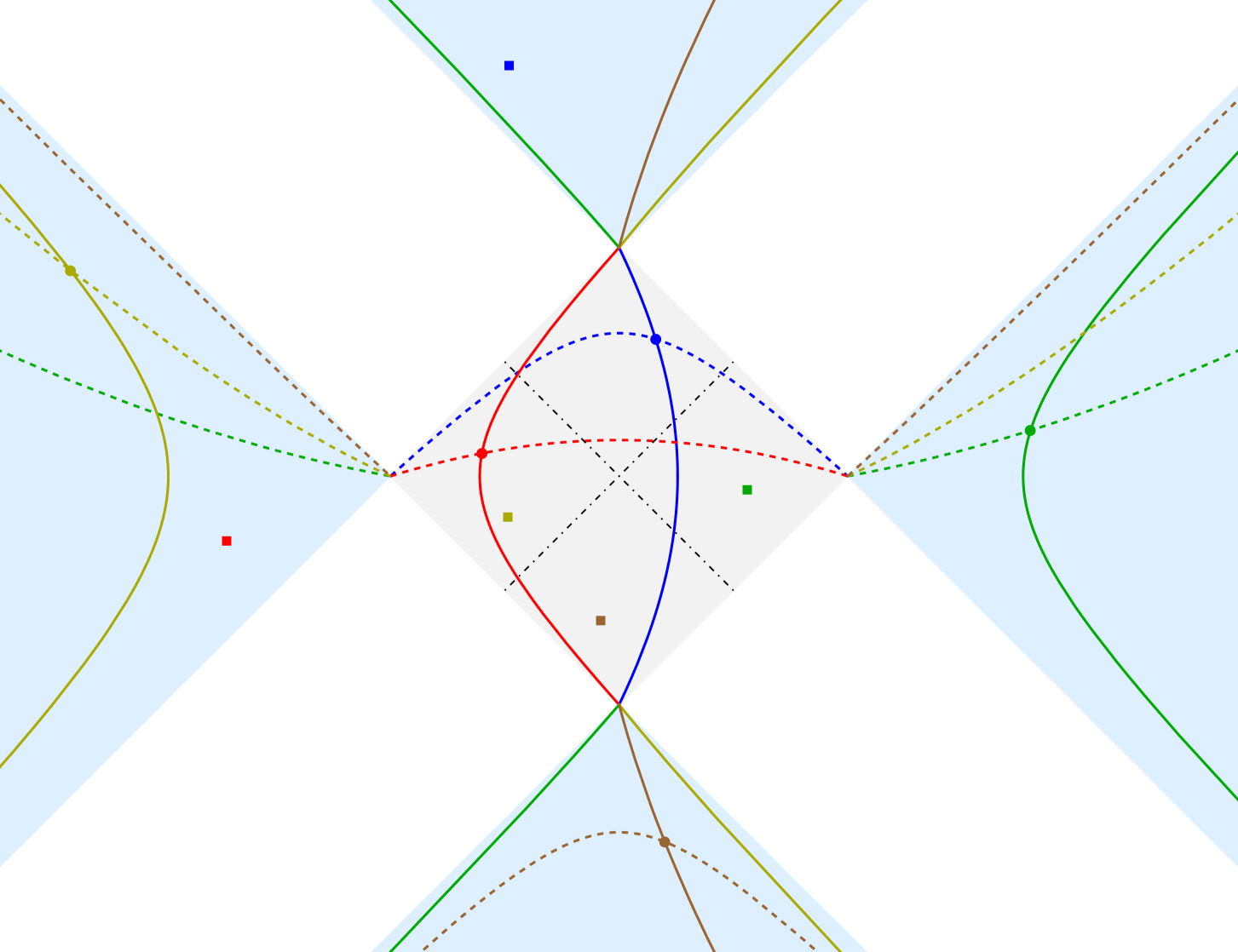
Figure 1: Modular trajectories generated by either the modular Hamiltonian (4.10) (solid lines) or the modular momentum (4.14) (dashed lines), obtained from (4.13) and (4.15) respectively. The coloured squares denote the images through the modular conjugation (4.22) of the spacetime points corresponding to the dots having the same colour. The dot dashed segments identify the partition $\mathcal{D}_{A}=\mathcal{D}_{\textrm{\tiny R}}\cup\mathcal{D}_{\textrm{\tiny L}}\cup\mathcal{D}_{\textrm{\tiny F}}\cup\mathcal{D}_{\textrm{\tiny P}}$ of the diamond $\mathcal{D}_{A}$.

The domain of dependence $\mathcal{D}_{A}$ of the interval $A$ is the diamond made by the points with light-cone coordinates $u_{\pm}\in A$ and it corresponds to the grey rhombus in Fig. 1. Its vertices $P_{a}$, $P_{b}$, $P_{+\infty}$ and $P_{-\infty}$ have light-cone coordinates $(u_{+},u_{-})\in\big{\{}(a,a)\,,(b,b)\,,(b,a)\,,(a,b)\big{\}}$ respectively. Let us introduce the partition of $\mathcal{D}_{A}$ provided by the light rays from its center $P_{c}$, whose light-cone coordinates are $u_{+}=u_{-}=\tfrac{a+b}{2}$ (see the dot-dashed segments in $\mathcal{D}_{A}$ in Fig. 1). This gives $\mathcal{D}_{A}=\mathcal{D}_{\textrm{\tiny R}}\cup\mathcal{D}_{\textrm{\tiny L}}\cup\mathcal{D}_{\textrm{\tiny F}}\cup\mathcal{D}_{\textrm{\tiny P}}$, where $\mathcal{D}_{i}$ belongs to the right wedge, the left wedge, the future cone and the past cone of $P_{c}$ for $i\in\big{\{}\textrm{R},\textrm{L},\textrm{F},\textrm{P}\big{\}}$ respectively. A modular trajectory (4.13) whose initial point corresponding to $\tau=0$ belongs to $\mathcal{D}_{A}$ entirely stays within $\mathcal{D}_{A}$, for any real value of $\tau$. In particular, its endpoints are the vertices $P_{+\infty}$ and $P_{-\infty}$, which are reached as $\tau\to+\infty$ and $\tau\to-\infty$ respectively. In Fig. 1 the red and blue solid lines are the modular trajectories whose initial points are the red and blue dots respectively. The modular trajectories whose initial point has light-cone coordinates $(u_{+},u_{-})$ such that $u_{\pm}\in A$ span the diamond $\mathcal{D}_{A}$.

As for region $\mathcal{R}_{A}$ made by the points with light-cone coordinates $u_{\pm}\in B$ (light blue region in Fig. 1), it can be naturally partitioned into four regions, i.e. $\mathcal{R}_{A}=\mathcal{R}_{\textrm{\tiny R}}\cup\mathcal{R}_{\textrm{\tiny L}}\cup\mathcal{R}_{\textrm{\tiny F}}\cup\mathcal{R}_{\textrm{\tiny P}}$, where $\mathcal{R}_{i}$ is the infinite region that shares a vertex of $\mathcal{D}_{A}$ with $\mathcal{D}_{i}$ and belongs to the right wedge, the left wedge, the future cone and the past cone of $P_{c}$ for $i\in\big{\{}\textrm{R},\textrm{L},\textrm{F},\textrm{P}\big{\}}$ respectively. The modular trajectories (4.13) with initial points at $\tau=0$ in $\mathcal{R}_{A}$ span the entire domain $\mathcal{R}_{A}$ (in Fig. 1, see e.g. the green, yellow and brown solid lines, whose initial points are the dots having the corresponding color). A modular trajectories which does not belong to the vertical line passing through $P_{+\infty}$ and $P_{-\infty}$ has a non trivial intersection with $\mathcal{R}_{\textrm{\tiny P}}$, $\mathcal{R}_{\textrm{\tiny F}}$ and either $\mathcal{R}_{\textrm{\tiny R}}$ or $\mathcal{R}_{\textrm{\tiny L}}$, depending on whether the $x$-coordinate of its initial point at $\tau=0$ (whose light-cone coordinate are $u_{\pm}$) is either $x>(a+b)/2$ or $x<(a+b)/2$ respectively (instead, the single modular trajectory belonging to the vertical line passing through $P_{+\infty}$ and $P_{-\infty}$ intersects $\mathcal{R}_{\textrm{\tiny P}}$ and $\mathcal{R}_{\textrm{\tiny F}}$ only). The two transitions from $\mathcal{R}_{\textrm{\tiny P}}$ to $\mathcal{R}_{i}$ and from $\mathcal{R}_{i}$ to $\mathcal{R}_{\textrm{\tiny F}}$, where $i\in\big{\{}\textrm{L},\textrm{R}\big{\}}$, occur at two finite values of $\tau$ given by $\tau_{\infty}(u_{+})$ and $\tau_{\infty}(u_{-})$, in terms of $\tau_{\infty}(u)$ introduced in (4.12) [29].

We remark that all the modular trajectories arrive to $P_{+\infty}$ and $P_{-\infty}$ as $\tau\to+\infty$ and $\tau\to-\infty$ respectively, independently of whether the initial point is either in $\mathcal{D}_{A}$ or in $\mathcal{R}_{A}$.

The modular momentum operator is obtained by specialising (3.40) to the case that we are investigating, finding

$$P\equiv\int_{-\infty}^{\infty}V(u_{+})\left[\,{\cal T}_{+}(u_{+})-\frac{\kappa\mu^{2}_{+}}{4\pi}\,\right]{\rm d}u_{+}-\int_{-\infty}^{\infty}V(u_{-})\left[\,{\cal T}_{-}(u_{-})-\frac{\kappa\mu^{2}_{-}}{4\pi}\,\right]{\rm d}u_{-}$$ (4.14)

where $V(u)$ has been introduced in (4.7). This operator provides a transformation of the fields that can be written by specialising the results of Sec. 3.3 to $V_{+}(u)=V_{-}(u)=V(u)$. The corresponding modular trajectories in the spacetime are obtained from (3.50) in the same way and the result reads

$$x(\lambda)=\frac{\zeta(\lambda,u_{+})+\zeta(\lambda,u_{-})}{2}\;\;\;\qquad\;\;\;t(\lambda)=\frac{\zeta(\lambda,u_{+})-\zeta(\lambda,u_{-})}{2}$$ (4.15)

where $\lambda\in{\mathbb{R}}$ and $(u_{+},u_{-})$ are the light-cone coordinates of the initial point at $\lambda=0$. The initial point can be either in $\mathcal{D}_{A}$ or in $\mathcal{R}_{A}$ and the entire modular trajectory (4.15) belongs to the same region for all finite real values of $\lambda$, reaching $P_{a}$ and $P_{b}$ as $\lambda\to-\infty$ and $\lambda\to+\infty$ respectively. In Fig. 1 the dashed curves we show some modular trajectories generated by the momentum operator, whose initial points are the dots with the same colour.

The above discussion is based on the fact that $V_{+}(u)=V_{-}(u)$, given by (4.7). Since the assumption $V_{+}=V_{-}$ has not been employed throughout Sec. 2, it is straightforward to extend our analysis to the boosted interval, which is characterised by two different bipartitions along the chiral directions, determined by the interval $(a_{+},b_{+})$ and $(a_{-},b_{-})$ for $u_{+}$ and $u_{-}$ directions respectively. When the CFT₂ is at finite densities, the modular Hamiltonian to consider is (2.6) with the following weight functions

$$V_{\pm}(u)\equiv 2\pi\,\frac{(b_{\pm}-u)(u-a_{\pm})}{b_{\pm}-a_{\pm}}=\frac{1}{w_{\pm}^{\prime}(u)}\;\;\;\qquad\;\;\;u\in(a_{\pm},b_{\pm})$$ (4.16)

where

$$w_{\pm}(u)\equiv\frac{1}{2\pi}\log\!\left(\!-\frac{u-a_{\pm}}{u-b_{\pm}}\right).$$ (4.17)

From Sec. 2.2, we have that the modular evolution of a primary chiral field is given by (2.18), where $\xi_{\pm}(\tau,u)$ is obtained by specifying (2.16) to this case. This leads to

$$\xi_{\pm}(\tau,u)=\frac{(b_{\pm}-u)\,a_{\pm}+(u-a_{\pm})\,b_{\pm}\,\mathrm{e}^{\pm 2\pi\tau}}{(b_{\pm}-u)+(u-a_{\pm})\,\mathrm{e}^{\pm 2\pi\tau}}$$ (4.18)

which reduce to (4.11) when $a_{+}=a_{-}$ and $b_{+}=b_{-}$, as expected. As for the modular evolution generated by the modular generalised momentum (3.40) defined through the weight functions (4.16) characterising the boosted interval, for a primary chiral field we find (3.48) with

$$\zeta_{\pm}(\lambda,u)=\frac{(b_{\pm}-u)\,a_{\pm}+(u-a_{\pm})\,b_{\pm}\,\mathrm{e}^{2\pi\lambda}}{(b_{\pm}-u)+(u-a_{\pm})\,\mathrm{e}^{2\pi\lambda}}\,.$$ (4.19)

From (4.18) and (4.19) it is straightforward to obtain the generalisation of Fig. 1 corresponding to a region of spacetime determined by two different intervals $(a_{+},b_{+})$ and $(a_{-},b_{-})$ along the chiral directions parameterised by $u_{+}$ and $u_{-}$ respectively.

Let us conclude this discussion with a brief comment on the relation between the operator (4.10) and the Tomita-Takesaki modular theory. Referring for details to [30], here we observe that the $K$-flow generated by the operator (4.10) is well defined for conformal fields with any dimension $h_{\pm}\geqslant 0$. With some abuse of terminology, such flow is usually called modular flow, although strictly speaking it can be associated with the Tomita-Takesaki theory only for quantum fields which are local, i.e. that either commute or anticommute at spacelike distances. In CFT, this is certainly the case for fields with dimensions $h_{\pm}\in\mathbb{Z}$ and $h_{\pm}\in{\mathbb{Z}}+\frac{1}{2}$. Hence, according to Sec. 2, the modular theory applies for the currents describing the transport of electric charge and helicity ($h_{\pm}=1$) and of energy ($h_{\pm}=2$). With the exception of Appendix B, in the following we focus on the modular properties of these currents.

4.3 Modular conjugation

The modular theory of Tomita and Takesaki [31, 1, 32, 33, 34] is constructed through the modular operator $e^{-K}$, written in terms of the full modular Hamiltonian, and the modular conjugation $J$, an antiunitary operator which leaves the state invariant and satisfies $J=J^{\ast}=J^{-1}$. For the bipartition and the state of the CFT we are considering, the modular conjugation has a geometric action implemented by the real function $\mathsf{j}:\mathbb{R}\rightarrow\mathbb{R}$ which can be obtained by setting $\tau=\pm\,{\rm i}/2$ in (4.11) and reads [1]

$$\mathsf{j}(u)\equiv\frac{a+b}{2}+\frac{\left(\frac{b-a}{2}\right)^{2}}{u-\frac{a+b}{2}}$$ (4.20)

which is a bijective and idempotent function sending $A$ onto $B$. The map (4.20) is invariant under $a\leftrightarrow b$ and satisfies $\mathsf{j}^{\prime}(u)<0$. We remark that (4.11) and (4.20) commute, namely

$$\mathsf{j}\big{(}\xi(\tau,u)\big{)}=\xi\big{(}\tau,\mathsf{j}(u)\big{)}\,.$$ (4.21)

Notice that $\mathsf{j}(u)$ in (4.20) becomes $\mathsf{j}(u)=2a-u$ as $b\to+\infty$ and $\mathsf{j}(u)=2b-u$ as $a\to-\infty$.

In Minkowski spacetime, the geometric action of the modular conjugation $J$ associated to the state and the bipartition we are investigating can be written through (4.20) as follows

$$\tilde{x}(x,t)\equiv\frac{\mathsf{j}(u_{+})+\mathsf{j}(u_{-})}{2}\;\;\;\qquad\;\;\;\tilde{t}(x,t)\equiv\frac{\mathsf{j}(u_{+})-\mathsf{j}(u_{-})}{2}\;.$$ (4.22)

In Fig. 1 the points labelled by coloured squares are the images through (4.22) of the points labelled by dots having the same colour. Considering the partitions of $\mathcal{D}_{A}$ and $\mathcal{R}_{A}$ introduced in Sec. 4.2, we have that, for any assigned $i\in\big{\{}\textrm{R},\textrm{L},\textrm{F},\textrm{P}\big{\}}$, the idempotent map (4.22) sends $\mathcal{D}_{i}$ onto $\mathcal{R}_{i}$ in a bijective way.

The image of the modular trajectories (4.13) through (4.22) has been studied e.g. in [29]. Within the context of the gauge/gravity correspondence, the holographic dual of (4.22) tor $t=0$ has been discussed [29, 35] by employing the geodesic bit threads [36, 37].

Considering a modular trajectory (4.13) in $\mathcal{D}_{A}$ with initial point $P\in\mathcal{D}_{A}$ having light-cone coordinates $(u_{+},u_{-})$, its image under (4.22) belongs to $\mathcal{R}_{A}$ and the spacetime coordinates of its generic point read [29]

$$\tilde{x}(\tau)=\frac{\mathsf{j}\big{(}\xi(\tau,u_{+})\big{)}+\,\mathsf{j}\big{(}\xi(-\tau,u_{-})\big{)}}{2}\;\;\;\qquad\;\;\;\tilde{t}(\tau)=\frac{\mathsf{j}\big{(}\xi(\tau,u_{+})\big{)}-\,\mathsf{j}\big{(}\xi(-\tau,u_{-})\big{)}}{2}$$ (4.23)

which can be written in an equivalent form by employing (4.21).

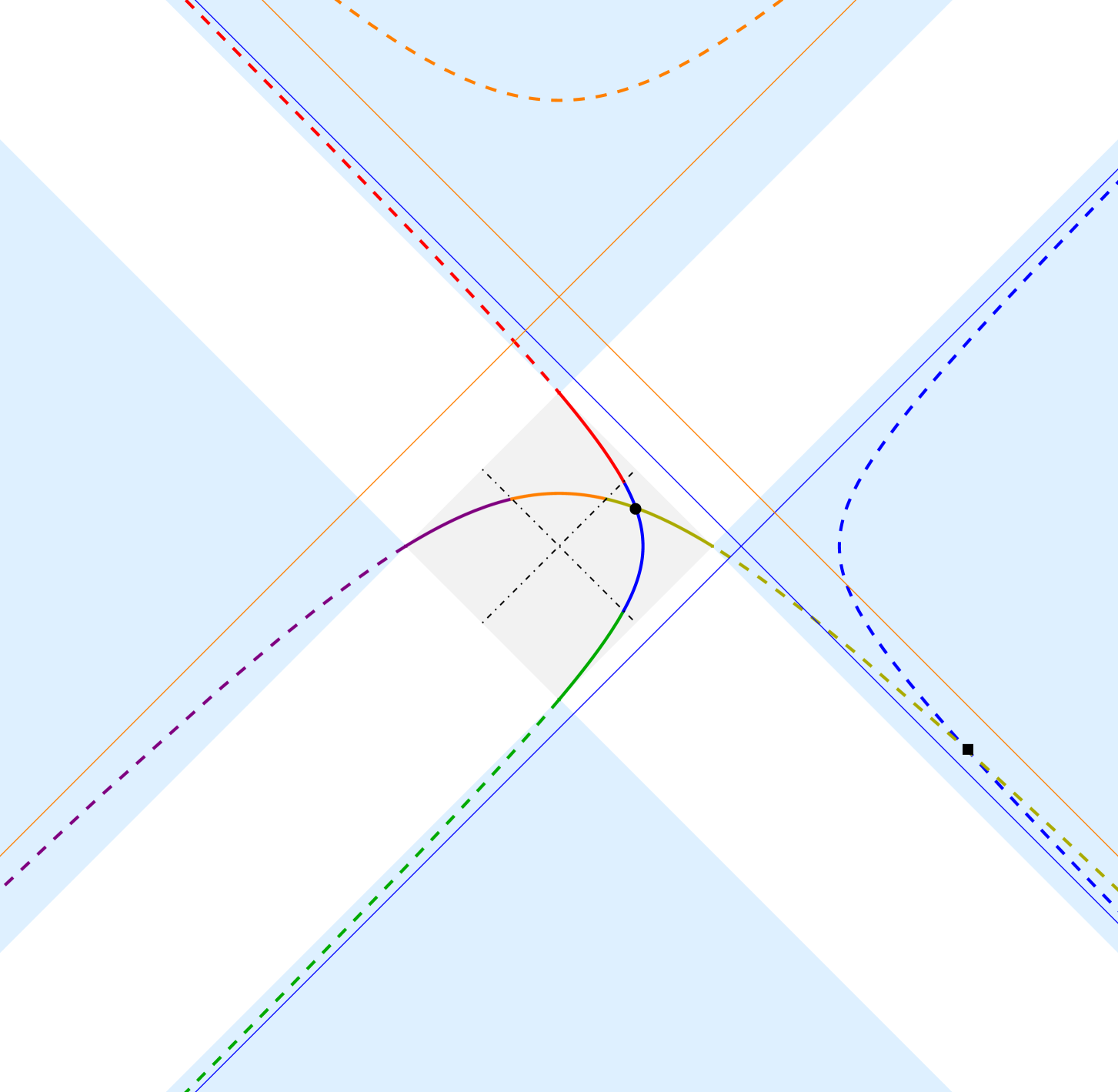
Figure 2: The modular hyperbolae $\mathcal{I}_{{}_{P}}$ in (4.24) correspond to the red, blue and green arcs, while the modular hyperbolae $\widetilde{\mathcal{I}}_{{}_{P}}$ in(4.27) is made by the purple, orange and dark yellow arcs. The asymptotes of $\mathcal{I}_{{}_{P}}$ and $\widetilde{\mathcal{I}}_{{}_{P}}$ are the orange and blue thin straight lines respectively.

In [29, 30] it has been observed that the union of the modular trajectory (4.13) in $\mathcal{D}_{A}$ and of the corresponding curve in $\mathcal{R}_{A}$ obtained through (4.23) provides the hyperbola $\mathcal{I}_{{}_{P}}$ defined as follows

$$\big{[}x(\tau)-x_{0}\big{]}^{2}-t(\tau)^{2}=\kappa^{2}\;\;\;\qquad\;\;\;\big{[}\tilde{x}(\tau)-x_{0}\big{]}^{2}-\tilde{t}(\tau)^{2}=\kappa_{0}^{2}$$ (4.24)

whose parameters are

$$x_{0}\equiv\frac{u_{+}\,u_{-}-a\,b}{u_{+}+u_{-}-(a+b)}\;\;\;\qquad\;\;\;\kappa_{0}\equiv\frac{\sqrt{(b-u_{+})(u_{+}-a)\,(b-u_{-})(u_{-}-a)}}{u_{+}+u_{-}-(a+b)}$$ (4.25)

in terms of the light-cone coordinates of the initial point $P$.

In Fig. 2, the point $P$ corresponds to the black dot and its modular trajectory has been partitioned into the the green, blue and red solid arcs, corresponding to the intersection of the modular trajectory with different $\mathcal{D}_{i}$, with $i\in\big{\{}\textrm{R},\textrm{L},\textrm{F},\textrm{P}\big{\}}$. The black square is the image of $P$ under (4.22) and the image of each arc through (4.22) is indicated by the dashed curve with the same colour. The asymptotes of the hyperbolae (4.24) are $t=x-x_{0}$ and $t=-x+x_{0}$ (see the blue solid thin straight lines in Fig. 2).

It is worth considering also the modular trajectory (4.15) provided by the evolution generated by the modular momentum operator (4.14) having the same point $P\in\mathcal{D}_{A}$ employed above as initial point at $\lambda=0$, where $\lambda\in{\mathbb{R}}$ is the modular parameter. In Fig. 2, this modular trajectory has been partitioned into the purple, orange and dark yellow solid arcs, which correspond to the intersection of the modular trajectory with different $\mathcal{D}_{i}$, with $i\in\big{\{}\textrm{R},\textrm{L},\textrm{F},\textrm{P}\big{\}}$. The image of the modular trajectory (4.15) through (4.22) belongs to $\mathcal{R}_{A}$ and reads

$$\tilde{x}(\lambda)=\frac{\mathsf{j}\big{(}\zeta(\lambda,u_{+})\big{)}+\,\mathsf{j}\big{(}\zeta(\lambda,u_{-})\big{)}}{2}\;\;\;\qquad\;\;\;\tilde{t}(\lambda)=\frac{\mathsf{j}\big{(}\zeta(\lambda,u_{+})\big{)}-\,\mathsf{j}\big{(}\zeta(\lambda,u_{-})\big{)}}{2}$$ (4.26)

In Fig. 2, the images under the inversion (4.22) of the solid arcs in purple, orange and dark yellow partitioning the modular trajectory obtained from (4.15) are the dashed arcs having the corresponding colour.

By adapting the construction of the hyperbola $\mathcal{I}_{{}_{P}}$ to the evolution generated by the modular momentum operator (4.14), here we observe that the union of the modular trajectory (4.15) and of its image under the map (4.22) described by (4.26) provide the hyperbola $\widetilde{\mathcal{I}}_{{}_{P}}$ given by

$$\big{[}\,t(\lambda)-t_{0}\,\big{]}^{2}-\left[\,x(\lambda)-\frac{a+b}{2}\,\right]^{2}\!=\lambda^{2}\;\;\qquad\;\;\big{[}\,\tilde{t}(\lambda)-t_{0}\,\big{]}^{2}-\left[\,\tilde{x}(\lambda)-\frac{a+b}{2}\,\right]^{2}\!=\tilde{\kappa}_{0}^{2}\phantom{xx}$$ (4.27)

where the parameters are

$$t_{0}\equiv\frac{\big{(}u_{+}-\tfrac{a+b}{2}\big{)}\big{(}u_{-}-\tfrac{a+b}{2}\big{)}-\big{(}\tfrac{b-a}{2}\big{)}^{2}}{u_{-}-u_{+}}\;\;\qquad\;\;\tilde{\kappa}_{0}\equiv\frac{\sqrt{(b-u_{+})(u_{+}-a)\,(b-u_{-})(u_{-}-a)}}{u_{+}-u_{-}}$$ (4.28)

in terms of the light-cone coordinates of the initial point $P$. These expressions are well defined whenever $u_{+}\neq u_{-}$; indeed, for $u_{+}=u_{-}$ the hyperbola $\widetilde{\mathcal{I}}_{{}_{P}}$ becomes the horizontal line $t=0$. The two hyperbolas $\mathcal{I}_{{}_{P}}$ and $\widetilde{\mathcal{I}}_{{}_{P}}$ intersect at $P\in\mathcal{D}_{A}$ and at its image under (4.22) in $\mathcal{R}_{A}$.

It is worth describing the action of the modular conjugation on the fields of the CFT considered in Sec. 2. In the literature, this transformation has been considered e.g. in [38, 39]. Since the geometric action of the modular conjugation is obtained from (4.11) at $\tau=\pm\,{\rm i}/2$, the action of $J$ on the basic fields of the CFT can be found by combining the fact that $J$ is antiunitary with (2.18), (2.20), (2.23) and (2.34). Thus, for the primaries we have

$$J\,\phi_{\pm}(u)\,J\,=\,\mathrm{e}^{\mp\mathrm{i}\mu_{\pm}(\,\mathsf{j}(u)-u)}\,\mathsf{j}^{\prime}(u)^{h_{\pm}}\,\phi^{\ast}_{\pm}(\,\mathsf{j}(u))$$ (4.29)

$$\rule{0.0pt}{14.22636pt}J\,\phi^{\ast}_{\pm}(u)\,J\,=\,\mathrm{e}^{\pm\mathrm{i}\mu_{\pm}(\,\mathsf{j}(u)-u)}\,\mathsf{j}^{\prime}(u)^{h_{\pm}}\,\phi_{\pm}(\,\mathsf{j}(u))$$ (4.30)

where, from (4.20), we have that $\mathsf{j}^{\prime}(u)<0$. We remark that $\mathsf{j}^{\prime}(u)\to-1$ as either $b\to+\infty$ or $a\to-\infty$. As for the currents and the operators (2.7) containing the energy-momentum tensor, which are hermitean operators, we find respectively

$$J\,j_{\pm}(u)\,J\,=\,\mathsf{j}^{\prime}(u)\,j_{\pm}(\,\mathsf{j}(u))-\frac{\kappa\mu_{\pm}}{2\pi}\left[\,1-\mathsf{j}^{\prime}(u)\,\right]$$ (4.31)

and

$$J\,\mathcal{T}_{\pm}(u)\,J\,=\,\mathsf{j}^{\prime}(u)^{2}\,\mathcal{T}_{\pm}(\,\mathsf{j}(u))+\frac{\kappa\mu_{\pm}^{2}}{4\pi}\left[\,1-\mathsf{j}^{\prime}(u)^{2}\,\right]$$ (4.32)

where in the last expression we used that the Schwarzian derivative (see (2.35)) of (4.20) vanishes identically, i.e. $\mathcal{S}_{u}[\,\mathsf{j}\,](u)=0$.

The transformation rule (4.32) can be employed to observe that

$$J\left(\,\int_{a}^{b}V(u)\,\mathcal{T}_{\pm}(u)\,{\rm d}u\right)J = \int_{a}^{b}\mathsf{j}^{\prime}(u)\,V(u)\,\mathcal{T}_{\pm}(\,\mathsf{j}(u))\,\mathsf{j}^{\prime}(u)\,{\rm d}u+\textrm{const}$$

$$= -\left[\,\int_{-\infty}^{a}\!\!V(u)\,\mathcal{T}_{\pm}(u)\,{\rm d}u+\int_{b}^{+\infty}\!\!V(u)\,\mathcal{T}_{\pm}(u)\,{\rm d}u\,\right]+\textrm{const}\hskip 28.45274pt$$

where we used that (4.7) and (4.20) satisfy the following identity

$$\mathsf{j}^{\prime}(u)\,V(u)=V(\,\mathsf{j}(u))\,.$$ (4.34)

By applying (4.3) to (4.6), it is straightforward to find that (4.9) can be written as $K_{B}=J\,K_{A}\,J$; hence the full modular Hamiltonian (4.10) can be equivalently expressed in the following suggestive form

$$K\equiv K_{A}\otimes\boldsymbol{1}_{B}-\boldsymbol{1}_{A}\otimes\big{(}J\,K_{A}\,J\big{)}$$ (4.35)

Since $J\,\Omega_{\mu_{\pm}}=\Omega_{\mu_{\pm}}$, taking the mean values of (4.29), (4.30), (4.31) and (4.32) in the l.h.s.’s one finds $\langle\phi_{\pm}(u)\rangle_{\mu_{\pm}}$, $\langle\phi^{\ast}_{\pm}(u)\rangle_{\mu_{\pm}}$, $\langle j_{\pm}(u)\rangle_{\mu_{\pm}}$ and $\langle{\cal T}_{\pm}(u)\rangle_{\mu_{\pm}}$ respectively. By using (4.1) in the corresponding r.h.s.’s, consistency is observed; indeed, the r.h.s.’s of the expressions in (4.1) are obtained.

The modular conjugation $J$ allows us to investigate the modular evolution in $\mathcal{R}_{A}$. Indeed, considering a chiral operator $\mathcal{O}_{\pm}(u)$ placed at $u\in B$, i.e. in the domain complementary to $A$ on the line, its modular evolution $\mathcal{O}_{\pm}(\tau,u)$ can be written as

$$\mathcal{O}_{\pm}(\tau,u)\,=\,{\rm e}^{\mathrm{i}K\tau}\,\mathcal{O}_{\pm}(u)\,{\rm e}^{-\mathrm{i}K\tau}\,=\,JJ\,{\rm e}^{\mathrm{i}K\tau}\,\mathcal{O}_{\pm}(u)\,{\rm e}^{-\mathrm{i}K\tau}JJ\,=\,J\left[\,{\rm e}^{\mathrm{i}K\tau}\big{(}J\,\mathcal{O}_{\pm}(u)\,J\,\big{)}\,{\rm e}^{-\mathrm{i}K\tau}\,\right]J$$ (4.36)

where we used that $J$ is idempotent and that $J\,{\rm e}^{\mathrm{i}K\tau}J={\rm e}^{\mathrm{i}K\tau}$ (see e.g. Eq. (V.2.9) of [1]). In the last expression of (4.36), the operator $J\,\mathcal{O}_{\pm}(u)\,J$ is located in $A$; hence the same holds for its modular evolution, which corresponds to the operator within the square brackets in the last expression of (4.36). In the Appendix E we have obtained explicit expressions for (4.36) when $\mathcal{O}_{\pm}$ is either $\phi_{\pm}$ or $j_{\pm}$ or $\mathcal{T}_{\pm}$, finding that the expressions for the modular evolutions given by (2.18), (2.20), (2.23) and (2.34) with $\xi_{\pm}(\tau,u)$ reported in (4.11) hold also when $u\in B$.

4.4 Modular correlators

The two-point functions of the primaries, of the currents and of the energy-momentum tensor along the modular evolution generated by the full modular Hamiltonian (4.10) can be written by combining the results discussed in Sec. 2.2 with the expressions reported in Sec. 4.1.

As for the one-point functions, from (4.1) we can take the mean values of (2.18), (2.20), (2.23) and (2.34) with $\xi_{\pm}(\tau,u)$ given by (4.11), finding that they are independent of $\tau$, i.e. $\langle\phi_{\pm}(u)\rangle_{\mu_{\pm}}=\langle\phi_{\pm}(\tau,u)\rangle_{\mu_{\pm}}$ for the primaries, $\langle j_{\pm}(u)\rangle_{\mu_{\pm}}=\langle j_{\pm}(\tau,u)\rangle_{\mu_{\pm}}$ for the currents and $\langle{\cal T}_{\pm}(u)\rangle_{\mu_{\pm}}=\langle{\cal T}_{\pm}(\tau,u)\rangle_{\mu_{\pm}}$ for the operators (2.7).

In order to investigate the modular two-point functions, we first observe that, when $u\neq v$ and $\tau_{1}\neq\tau_{2}$ are real, for (4.11) we have

$$\frac{\partial_{u}\xi(\tau_{1},u)\,\partial_{v}\xi(\tau_{2},v)}{\big{[}\xi(\tau_{1},u)-\xi(\tau_{2},v)\big{]}^{2}}=\bigg{(}\frac{R(\tau_{12};u,v)}{u-v}\bigg{)}^{2}$$ (4.37)

where we have introduced

$$R(\tau;u,v)\equiv\frac{{\rm e}^{2\pi w(u)}-{\rm e}^{2\pi w(v)}}{{\rm e}^{2\pi w(u)+\pi\tau}-{\rm e}^{2\pi w(v)-\pi\tau}}\,=\,\frac{(u-a)(v-b)-(u-b)(v-a)}{(u-a)(v-b)\,{\rm e}^{\pi\tau}-(u-b)(v-a)\,{\rm e}^{-\pi\tau}}$$ (4.38)

which satisfies

$$R(\tau=0;u,v)=1\;\qquad\;R(-\tau;v,u)=R(\tau;u,v)\;\qquad\;R(\tau+{\rm i}\,;u,v)=-R(-\tau;v,u)$$ (4.39)

In the derivation of (4.37) we used that

$$\xi(\tau_{1},u)-\xi(\tau_{2},v)=\frac{p(\tau_{1},u)\,p(\tau_{2},v)}{R(\tau_{12};u,v)}\;(u-v)$$ (4.40)

in terms of (4.38) and of

$$p(\tau,u)\equiv\frac{(b-a)\,{\rm e}^{\pi\tau}}{b-u+(u-a)\,{\rm e}^{2\pi\tau}}\;\;\;\qquad\;\;\;q(\tau,u)\equiv b-u+(u-a)\,{\rm e}^{2\pi\tau}\,.$$ (4.41)

The dependence on $\tau_{12}$ in (4.37), which is not evident in the l.h.s., occurs because the product $q(\tau_{1},u)\,q(\tau_{2},v)$ simplifies in the ratio (see (4.40)). Notice that ${\rm e}^{2\pi w(u)}$ in (4.37) is well defined for $u\in{\mathbb{R}}$, although $w(u)$ in (4.8) holds for $u\in A$. Moreover, we remark that (4.37) is invariant under the simultaneous exchange $a\leftrightarrow b$ and $\tau_{1}\leftrightarrow\tau_{2}$.

For the primaries $\phi_{\pm}$, from (2.18), (2.20), (4.1), (4.2) and (4.37), one finds the following modular correlators

$$\langle\phi_{\pm}^{*}(\tau_{1},u)\,\phi_{\pm}(\tau_{2},v)\rangle_{\mu_{\pm}}^{\textrm{\tiny con}} =$$

$$\hskip-99.58464pt=\,{\rm e}^{\mp{\rm i}\mu_{\pm}[\xi_{\pm}(\tau_{1},u)-\xi_{\pm}(\tau_{2},v)-u+v]}\big{[}\partial_{u}\xi_{\pm}(\tau_{1},u)\,\partial_{v}\xi_{\pm}(\tau_{2},v)\big{]}^{h_{\pm}}\langle\phi_{\pm}^{*}\big{(}\xi_{\pm}(\tau_{1},u)\big{)}\,\phi_{\pm}\big{(}\xi_{\pm}(\tau_{2},v)\big{)}\rangle_{\mu_{\pm}}$$

$$\hskip-99.58464pt=\,\frac{{\rm e}^{\pm{\rm i}\mu_{\pm}(u-v)}}{2\pi\,{\rm e}^{\pm{\rm i}\pi h_{\pm}}}\;W_{\pm}(\pm\tau_{12};u,v)^{2h_{\pm}}$$ (4.42)

and

$$\langle\phi_{\pm}(\tau_{1},u)\,\phi^{*}_{\pm}(\tau_{2},v)\rangle_{\mu_{\pm}}^{\textrm{\tiny con}}=\,\frac{{\rm e}^{\mp{\rm i}\mu_{\pm}(u-v)}}{2\pi\,{\rm e}^{\pm{\rm i}\pi h_{\pm}}}\;W_{\pm}(\pm\tau_{12};u,v)^{2h_{\pm}}$$ (4.43)

where we have introduced

$$W_{\pm}(\tau;u,v)\,\equiv\,\frac{{\rm e}^{2\pi w(u)}-{\rm e}^{2\pi w(v)}}{u-v}\;\frac{1}{{\rm e}^{2\pi w(u)+\pi\tau}-{\rm e}^{2\pi w(v)-\pi\tau}\mp{\rm i}\varepsilon}\;.$$ (4.44)

When either $u\neq v$ or $\tau\neq 0$, we can set $\varepsilon=0$ and $W_{\pm}(\tau;u,v)$ becomes

$$W(\tau;u,v)\equiv\frac{R(\tau;u,v)}{u-v}$$ (4.45)

in terms of (4.38). Notice that the Hilbert space structure implies that (4.4) satisfies

$$\langle\phi_{\pm}^{*}(\tau_{1},u)\,\phi_{\pm}(\tau_{2},v)\rangle_{\mu_{\pm}}^{\textrm{\tiny con}}=\overline{\langle\phi^{\ast}_{\pm}(\tau_{2},v)\,\phi_{\pm}(\tau_{1},u)\rangle_{\mu_{\pm}}^{\textrm{\tiny con}}}$$ (4.46)

where the overline denotes the complex conjugation.

As for the currents $j_{\pm}$, from (2.23), (4.1), (4.3) and (4.37), their modular correlators read

$$\langle j_{\pm}(\tau_{1},u)\,j_{\pm}(\tau_{2},v)\rangle_{\mu_{\pm}}^{\textrm{\tiny con}} = \big{[}\partial_{u}\xi_{\pm}(\tau_{1},u)\,\partial_{v}\xi_{\pm}(\tau_{2},v)\big{]}\,\langle j_{\pm}\big{(}\xi_{\pm}(\tau_{1},u)\big{)}\,j_{\pm}\big{(}\xi_{\pm}(\tau_{2},v)\big{)}\rangle_{\mu_{\pm}}$$

$$= \frac{\kappa}{4\pi^{2}}\,W_{\pm}(\pm\tau_{12};u,v)^{2}\,.$$ (4.47)

Similarly, for the modular correlators of the operators (2.7), which contains the energy-momentum tensor, from (2.34), (4.1), (4.4) and (4.37), we find

$$\langle{\cal T}_{\pm}(\tau_{1},u)\,{\cal T}_{\pm}(\tau_{2},v)\rangle_{\mu_{\pm}}^{\textrm{\tiny con}} = \big{[}\partial_{u}\xi_{\pm}(\tau_{1},u)\,\partial_{v}\xi_{\pm}(\tau_{2},v)\big{]}^{2}\,\langle{\cal T}_{\pm}\big{(}\xi_{\pm}(\tau_{1},u)\big{)}\,{\cal T}_{\pm}\big{(}\xi_{\pm}(\tau_{2},v)\big{)}\rangle_{\mu_{\pm}}$$

$$= \frac{c}{8\pi^{2}}\,W_{\pm}(\pm\tau_{12};u,v)^{4}\,.$$ (4.48)

We remark that these modular correlators are functions of $\tau_{12}$ which depend on $t_{1}$ and $t_{2}$ separately; hence the modular energy is conserved along the modular evolution (see Sec. 3.2), while the conventional energy is not. Furthermore, according to the discussion reported at the end of Sec. 4.3 and in the Appendix E, we have that the expressions (4.4), (4.43), (4.4) and (4.4) for the modular correlators hold for any $u,v\in{\mathbb{R}}$.

Since for (4.44) the following property holds

$$W_{\pm}(\tau+{\rm i};u,v)=W_{\pm}(\tau-{\rm i};u,v)=W_{\pm}(-\tau;v,u)$$ (4.49)

the modular correlators (4.4), (4.43), (4.4) and (4.4) satisfy the KMS condition with modular inverse temperature $\tilde{\beta}=1$. This is a characterising feature of the modular correlators that exposes the thermal nature of the modular evolution. Furthermore, the validity of this condition confirms the expression (4.6) for the modular Hamiltonian (this criterion has been adopted e.g. in [40] to confirm the expression of the modular Hamiltonian of disjoint intervals on the line for the massless Dirac field in the ground state, found in [41]).

In the Appendix D we also provide a consistency check for (4.4) based on the modular reflection positivity property (see e.g. [38]).

Let us highlight that, when $\tau\neq 0$, the limit $v\to u$ of (4.44) is well defined and reads

$$\lim_{v\to u}W_{\pm}(\tau;u,v)=\frac{\pi}{V(u)\,\sinh(\pi\tau\mp{\rm i}\varepsilon)}\;.$$ (4.50)

This observation will be employed in Sec. 5.3 in a crucial way.

From the properties of the modular conjugation, for a chiral operator $\mathcal{O}_{\pm}$ we have

$$\langle\mathcal{O}_{\pm}^{*}(\tau_{1},u)\,\mathcal{O}_{\pm}(\tau_{2},v)\rangle_{\mu_{\pm}}^{\textrm{\tiny con}}=\langle\big{[}J\,\mathcal{O}^{\ast}_{\pm}(\tau_{2},v)\,J\big{]}\big{[}J\,\mathcal{O}_{\pm}(\tau_{1},u)\,J\big{]}\rangle_{\mu_{\pm}}^{\textrm{\tiny con}}$$ (4.51)

By employing the following identity

$$W_{\pm}(\tau,u,v)^{2}=\mathsf{j}^{\prime}(u)\,\mathsf{j}^{\prime}(v)\,W_{\pm}(-\tau,\mathsf{j}(v),\mathsf{j}(u))^{2}$$ (4.52)

we checked that the r.h.s.’s of (4.29), (4.30) (4.31) and (4.32) are consistent with (4.51).

The analyses discussed above can be extended to investigate the correlators of the fields whose evolution is determined by the momentum operator (see (4.14)-(4.15) and Sec. 3.3). It is straightforward to adapt the expressions (4.4), (4.43), (4.4) and (4.4) to these flows, finding correlators that satisfy the corresponding KMS condition, whose validity is based on the property (4.49) for (4.44).

5 Modular transport and fluctuations

In this section we consider the modular evolution $\mathcal{O}(\tau;x,t)\equiv{\rm e}^{{\rm i}\tau K}\mathcal{O}(x,t)\,{\rm e}^{-{\rm i}\tau K}$ of some observables $\mathcal{O}$ (essentially currents and densities) of the CFT in the finite density representation and for the bipartition given by an interval on the line. In unitary quantum field theory, the sequence of connected correlation functions $\big{\{}\langle\mathcal{O}(\tau_{1};x_{1},t_{1})\,...\,\mathcal{O}(\tau_{n};x_{n},t_{n})\rangle_{\mu}^{\textrm{\tiny con}}\big{\}}$ provides the cumulants of a probability distribution (see e.g. [1]). Hereafter the notation $\langle\,\dots\rangle_{\mu}$ denotes that both $\langle\,\dots\rangle_{\mu_{+}}$ and $\langle\,\dots\rangle_{\mu_{-}}$ are employed. When $\mathcal{O}$ is a current, this distribution fully describes the microscopic transport properties of the associated charge. For $n=1$ and $n=2$ one gets respectively the mean value and the quadratic fluctuations (quantum noise) of the current. In the following we consider operators whose one-point function $\langle\mathcal{O}(\tau;x,t)\rangle_{\mu}$ is independent of $\tau$, as discussed in Sec. 4.4.

5.1 Charge and helicity transport

The mean values of the charge currents in (3.6) and (3.9) in the finite density representation of the CFT on the line can be written by using (4.1) and specialising the velocities to $V_{+}(u)=V_{-}(u)$ given by (4.7). The result is

$$\langle j_{x}(\tau;x,t)\rangle_{\mu} = \frac{\kappa}{2\pi}\,\big{[}\mu_{+}V(u_{+})-\mu_{-}V(u_{-})\big{]}$$ (5.1)

$$\rule{0.0pt}{17.07182pt}\langle j_{t}(\tau;x,t)\rangle_{\mu} = \frac{\kappa}{2\pi}\,\big{[}\mu_{+}V(u_{+})+\mu_{-}V(u_{-})\big{]}\,.$$ (5.2)

We remark that, instead, the mean values of the operators (3.12) and (3.13) vanish identically.

The mean values of the helicity currents (3.22) are obtained in the same way and read

$$\langle k_{x}(\tau;x,t)\rangle_{\mu} = \frac{\kappa}{2\pi}\,\big{[}\mu_{+}V(u_{+})+\mu_{-}V(u_{-})\big{]}$$ (5.3)

$$\rule{0.0pt}{17.07182pt}\langle k_{t}(\tau;x,t)\rangle_{\mu} = \frac{\kappa}{2\pi}\,\big{[}\mu_{+}V(u_{+})-\mu_{-}V(u_{-})\big{]}\,.$$ (5.4)

These mean values for the charge currents and for the helicity currents are independent of $\tau$ and the event with spacetime coordinates $(x,t)$ corresponds to the initial point of the modular evolution; hence $(x,t)\in\mathcal{D}_{A}\cup\mathcal{R}_{A}$. We find it worth introducing the smooth planar vector fields $\boldsymbol{j}(x,t)\equiv\big{(}\langle j_{x}(\tau;x,t)\rangle_{\mu}\,,\langle j_{t}(\tau;x,t)\rangle_{\mu}\big{)}$ and $\boldsymbol{k}(x,t)\equiv\big{(}\langle k_{x}(\tau;x,t)\rangle_{\mu}\,,\langle k_{t}(\tau;x,t)\rangle_{\mu}\big{)}$ for $(x,t)\in\mathcal{D}_{A}\cup\mathcal{R}_{A}$. Despite the fact that these vector fields are defined in $\mathcal{D}_{A}\cup\mathcal{R}_{A}$, it is natural to extend them to the entire Minkowski spacetime and in the following such extension will be mainly explored. In Fig. 3 and Fig. 4 the vector fields $\boldsymbol{j}(x,t)$ and $\boldsymbol{k}(x,t)$ are displayed for a specific choice of the parameters (see the caption of Fig. 3). In particular, in the left panels $\mu_{+}=\mu_{-}$, while $\mu_{+}\neq\mu_{-}$ in the right panels. Moreover, in Fig. 3 the top panels show $\boldsymbol{j}(x,t)$ for $(x,t)\in\mathcal{D}_{A}\cup\mathcal{R}_{A}$, while in the bottom panels the corresponding extensions to the entire Minkowski spacetime are displayed.

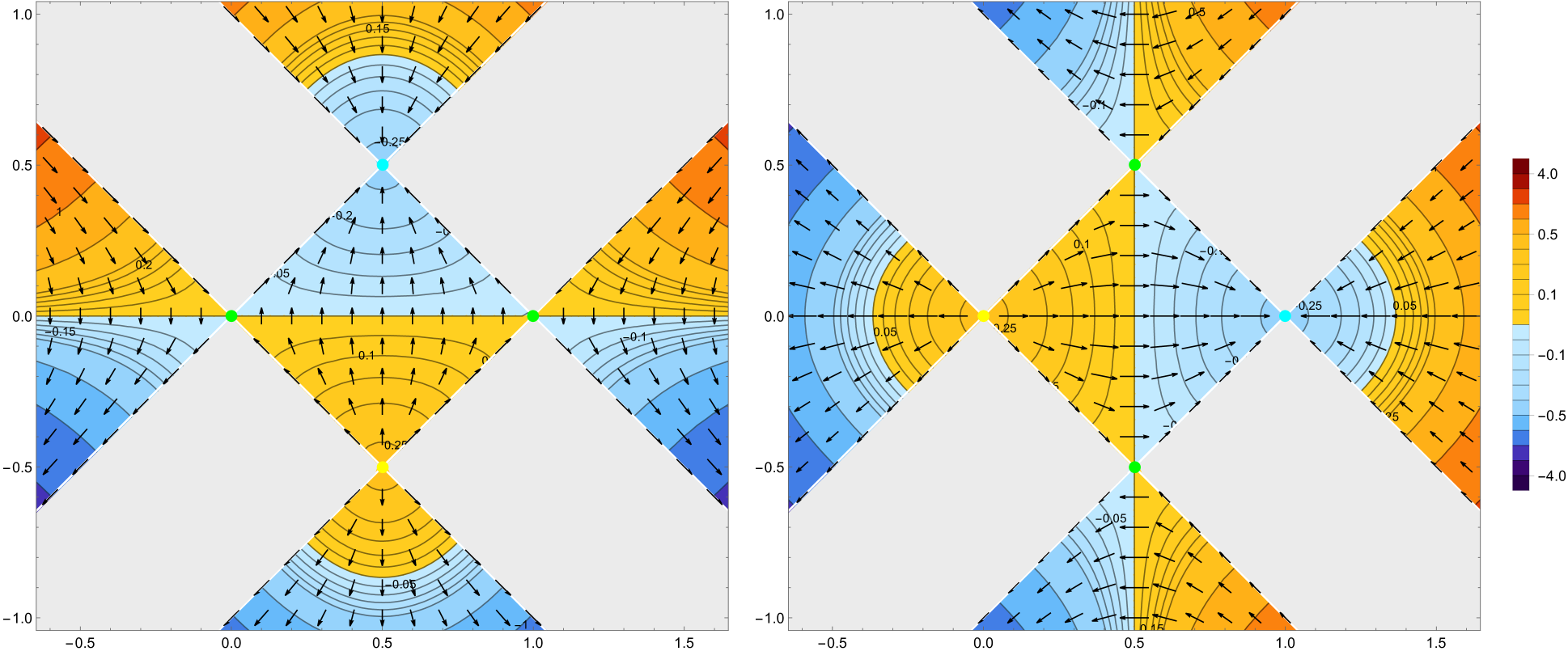
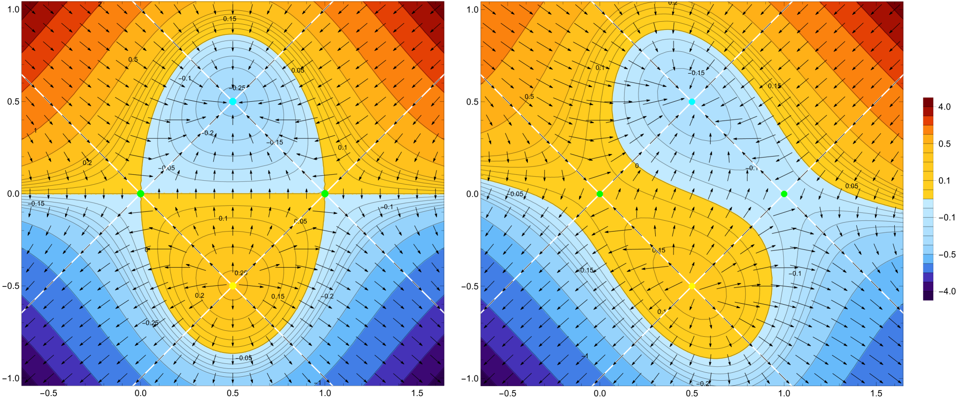
Figure 3: Vector fields for the mean values of the charge currents (5.1) and (5.2), whose potential is the first expressions in (5.12). The interval is $A=[0,1]$ on the line and the CFT has $c=1$, $\kappa=3$ and either equal chemical potentials $\mu_{+}=\mu_{-}=0.52$ (left panels) or different chemical potentials $\mu_{+}=0.52$ and $\mu_{-}=0.22$ (right panels). In the top panels the initial point $(x,t)\in\mathcal{D}_{A}\cup\mathcal{R}_{A}$, while in the bottom panels the vector field $\boldsymbol{j}(x,t)$ is extended to the entire Minkowski spacetime.

Two-dimensional vector fields have been largely explored [42, 43]. For instance, it is insightful to consider the critical points (also called singular points in the mathematical literature) of the vector field, i.e. the points where it vanishes. By construction, the critical points of both the vector fields $\boldsymbol{j}(x,t)$ and $\boldsymbol{k}(x,t)$ extended to the entire Minkowski spacetime are isolated points located in the vertices of the diamond $\mathcal{D}_{A}$, i.e. $P_{a}$, $P_{b}$, $P_{+\infty}$ and $P_{-\infty}$, whose light-cone coordinates are $(u_{+},u_{-})\in\big{\{}(a,a)\,,(b,b)\,,(b,a)\,,(a,b)\big{\}}$ respectively (see the coloured dots in Fig. 3 and Fig. 4), which are obtained by combining the zeros of the function $V(u)$ in (4.7). Since $a$ and $b$ are zeros of (4.7) of order $1$, all these critical points have multiplicity $1$.

The Poincaré index is a useful tool to study smooth vector fields $\boldsymbol{v}\equiv(v_{x},v_{t})$ with isolated zeros. Given a smooth closed curve $\gamma$ where the vector field is not vanishing, the Poincaré index of $\gamma$ relative to the vector field $\boldsymbol{v}$ can be computed as follows

$$\mathcal{I}[\boldsymbol{v}](\gamma)\equiv\frac{1}{2\pi}\oint_{\gamma}\frac{v_{t}\,{\rm d}v_{x}-v_{x}\,{\rm d}v_{t}}{v_{x}^{2}+v_{t}^{2}}$$ (5.5)

and it corresponds to the number of rotations in the positive (counterclockwise) direction that the vector field performs when we go around $\gamma$ once. The index $\mathcal{I}_{P}$ of a critical point $P$ is the Poincaré index of a closed smooth curve that encloses only $P$; hence it is determined by the behaviour of the vector field nearby $P$. Depending on such behaviour, $P$ is a critical point of certain type (e.g. either a node or a center or a focus or a saddle or something else). A node contains all the nearby trajectories and it is either stable or unstable, depending on whether all the trajectories move away from the point. A saddle has two transversal trajectories called separatices, one of which is ingoing and the other outgoing, while the other trajectories behave like a family of hyperbolas whose asymptotes are the separatrices. A node has Poincaré index $+1$ (like a focus and a center), while a saddle has Poincaré index $-1$. The vector fields $\boldsymbol{j}(x,t)$ and $\boldsymbol{k}(x,t)$ display two nodes, one stable and one unstable, and two saddles (in the bottom panels of Fig. 3 and Fig. 4, see the cyan dot, the yellow dot and the green dots respectively).

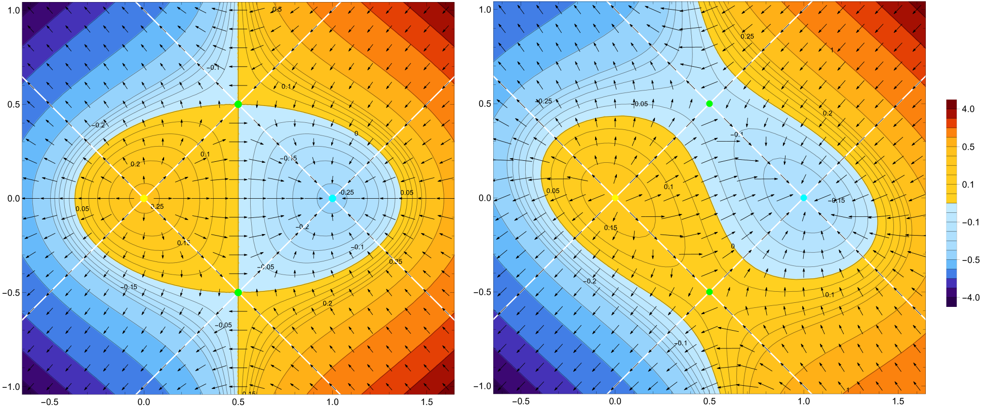
Figure 4: Vector fields for the mean values of the helicity currents (5.3) and (5.4), whose potential is the second expressions in (5.12), for either equal (left panel) or different (right panel) chemical potentials, in the same setup of Fig. 3.

Various theorems about the sum of the indices for smooth vector fields with isolated zeros have been established [42]. For instance, the index of a closed curve is equal to the sum of the indices of the critical points enclosed by the curve. A fundamental result in this context is the Poincaré-Hopf theorem, which claims that the sum of the indices of all the isolated critical points of a vector field on a two-dimensional compact manifold is independent of the vector field and equal to the Euler characteristic of the manifold. For the vector fields $\boldsymbol{j}(x,t)$ and $\boldsymbol{k}(x,t)$, which are defined on the plane, the sum of the indices of all the critical points is zero. These vector fields can be mapped to the Riemann sphere through the stereographic projection and the resulting vector fields on this compact manifold must have a critical point with Poincaré index $+2$ at the north pole, which corresponds to infinity on the plane.

By employing the definitions in (3.52), from (5.1)-(5.2) and (5.3)-(5.4) we introduce the local conductivities respectively as

$$\boldsymbol{\sigma}_{j,e} \equiv \partial_{\mu_{e}}\boldsymbol{j}(x,t)=\frac{\kappa}{4\pi}\,\Big{(}V(u_{+})-V(u_{-})\,,\,V(u_{+})+V(u_{-})\Big{)}$$ (5.6)

$$\rule{0.0pt}{19.91684pt}\boldsymbol{\sigma}_{j,h} \equiv \partial_{\mu_{h}}\boldsymbol{j}(x,t)=\frac{\kappa}{4\pi}\,\Big{(}V(u_{+})+V(u_{-})\,,\,V(u_{+})-V(u_{-})\Big{)}$$ (5.7)

and

$$\boldsymbol{\sigma}_{k,e}\equiv\partial_{\mu_{e}}\boldsymbol{k}(x,t)=\boldsymbol{\sigma}_{j,h}\;\;\;\qquad\;\;\;\boldsymbol{\sigma}_{k,h}\equiv\partial_{\mu_{h}}\boldsymbol{k}(x,t)=\boldsymbol{\sigma}_{j,e}\,.$$ (5.8)

These four local conductivities are independent of $\tau$; hence their Fourier transform gives only a Dirac delta term.

In order to understand the nature of the modular transport, let us consider

$$\int_{0}^{\tau}\boldsymbol{j}(x,t)\,{\rm d}\tilde{\tau}=\boldsymbol{j}(x,t)\,\tau\;\;\;\qquad\;\;\;\int_{0}^{\tau}\boldsymbol{k}(x,t)\,{\rm d}\tilde{\tau}=\boldsymbol{k}(x,t)\,\tau\,.$$ (5.9)

These linear growths tell us that the modular transport is ballistic (see e.g. [44]). We remark that the linear response approximation is not employed here.

A vector field $\boldsymbol{v}$ has vanishing curl when its components satisfy $\partial_{t}v_{x}-\partial_{x}v_{t}=0$ and this feature implies that it can be written as the gradient of the potential $\mathsf{W}$, namely $v_{\mu}=-\,\partial_{\mu}\mathsf{W}$.

Both the vector fields $\boldsymbol{j}(x,t)$ and $\boldsymbol{k}(x,t)$ have vanishing curl and therefore the corresponding potentials $\mathsf{W}_{j}(x,t)$ and $\mathsf{W}_{k}(x,t)$ respectively can be obtained. Indeed, we find that

$$\langle j_{x}(\tau;x,t)\rangle_{\mu}=-\,\partial_{x}\mathsf{W}_{j}(x,t)\;\;\;\qquad\;\;\;\langle j_{t}(\tau;x,t)\rangle_{\mu}=-\,\partial_{t}\mathsf{W}_{j}(x,t)$$ (5.10)

and

$$\langle k_{x}(\tau;x,t)\rangle_{\mu}=-\,\partial_{x}\mathsf{W}_{k}(x,t)\;\;\;\qquad\;\;\;\langle k_{t}(\tau;x,t)\rangle_{\mu}=-\,\partial_{t}\mathsf{W}_{k}(x,t)$$ (5.11)

where the potentials $\mathsf{W}_{j}$ and $\mathsf{W}_{k}$ are defined respectively as

$$\mathsf{W}_{j}(x,t)\equiv\frac{\kappa}{2\pi}\big{[}\mu_{+}g(u_{+})-\mu_{-}g(u_{-})\big{]}\;\;\;\qquad\;\;\;\mathsf{W}_{k}(x,t)\equiv\frac{\kappa}{2\pi}\big{[}\mu_{+}g(u_{+})+\mu_{-}g(u_{-})\big{]}$$ (5.12)

in terms of

$$g(u)\equiv\frac{2\pi}{3(b-a)}\left(u-\frac{a+b}{2}\right)\left(u^{2}-(a+b)\,u-\frac{a^{2}-4ab+b^{2}}{2}\,\right).$$ (5.13)

The arbitrary additive constants in (5.12) have been fixed by imposing the vanishing condition at the center of $\mathcal{D}_{A}$ for both these potentials; indeed (5.13) has a zero at $u=(a+b)/2$. We remark that (5.1)-(5.2), (5.3)-(5.4) are consistent with (5.10) and (5.11) because

$$-\,\partial_{u}g(u)=V(u)\,.$$ (5.14)

Given a curve $\gamma$ (not necessarily closed) parameterised by $s$, let us denote the line integral of the vector field $\boldsymbol{v}$ along $\gamma$ and the flux of $\boldsymbol{v}$ through $\gamma$ respectively as

$$\mathcal{L}[\boldsymbol{v}](\gamma)\equiv\int_{\gamma}\boldsymbol{v}\cdot\hat{\boldsymbol{\tau}}\,{\rm d}s\;\;\;\qquad\;\;\;\mathcal{F}[\boldsymbol{v}](\gamma)\equiv\int_{\gamma}\boldsymbol{v}\cdot\hat{\boldsymbol{n}}\,{\rm d}s$$ (5.15)

where $\hat{\boldsymbol{\tau}}$ and $\hat{\boldsymbol{n}}$ are the unit vectors which are respectively tangent and normal to $\gamma$.

We highlight the vanishing of the fluxes of the vector fields $\boldsymbol{j}(x,t)$ and $\boldsymbol{k}(x,t)$ through the straight white lines in Fig. 3 and Fig. 4, which identify the diamond $\mathcal{D}_{A}$ and the region $\mathcal{R}_{A}$ (i.e. the grey and light blue regions in Fig. 1). This can be shown by observing that the absolute value of the ratio of theirs components is equal to one along these lines. This absence of flux naturally suggests to consider the total charges in the diamond $\mathcal{D}_{A}$. In the finite density representation, by using (4.1) and (3.52), for the mean values of (3.17) and (3.23) we find respectively

$$\langle Q_{A}\rangle_{\mu}=\,-\frac{\kappa}{4\pi}\,\mu_{e}\,\ell^{2}\;\;\;\qquad\;\;\;\langle\widetilde{Q}_{A}\rangle_{\mu}=\,-\frac{\kappa}{4\pi}\,\mu_{h}\,\ell^{2}\,.$$ (5.16)

A crucial feature of $\boldsymbol{j}(x,t)$ and $\boldsymbol{k}(x,t)$ is that they are curl free vector fields. The Green theorem implies that any line integral of a curl free vector field along a closed curve vanishes; hence, all the line integrals along curves anchored to the same endpoints provide the same result given by the difference between the values of the potential at these endpoints. In our case, we find it worth considering the lines anchored to the opposite vertices of $\mathcal{D}_{A}$ and, among them, the convenient representatives to choose are the horizontal segment $A=\{(x,t=0)\,;\,a\leqslant x\leqslant b\}$ along the real axis, whose endpoints are $P_{a}$ and $P_{b}$, and the vertical segment $\tilde{A}=\{(x=\tfrac{a+b}{2},t)\,;\,-\tfrac{b-a}{2}\leqslant t\leqslant\tfrac{b-a}{2}\}$ on the imaginary axis, whose endpoints are $P_{-\infty}$ and $P_{+\infty}$. Given a smooth curves $\gamma(P_{1}\to P_{2})$ starting in $P_{1}$ and ending in $P_{2}$ and a vector field $\boldsymbol{v}(x,t)$, let us denote by $\mathcal{L}[\boldsymbol{v}]\big{(}\gamma(P_{1}\to P_{2})\big{)}$ the line integral of $\boldsymbol{v}(x,t)$ along $\gamma(P_{1}\to P_{2})$ and by $\mathcal{F}[\boldsymbol{v}]\big{(}\gamma(P_{1}\to P_{2})\big{)}$ its flux through $\gamma(P_{1}\to P_{2})$. When $\boldsymbol{v}(x,t)$ is curl free, $\mathcal{L}[\boldsymbol{v}]\big{(}\gamma(P_{1}\to P_{2})\big{)}$ depends only on the endpoints $P_{1}$ and $P_{2}$. For the vector field $\boldsymbol{j}(x,t)$ in (5.1)-(5.2), these line integrals can be written in terms of the mean values of total charges (5.16) as follows

$$\mathcal{L}[\boldsymbol{j}]\big{(}\gamma(P_{a}\to P_{b})\big{)} = \mathsf{W}_{j}\big{|}_{P_{a}}-\mathsf{W}_{j}\big{|}_{P_{b}}\,=\,-\frac{2\pi}{3}\,\langle\widetilde{Q}_{A}\rangle_{\mu}$$ (5.17)

$$\rule{0.0pt}{19.91684pt}\mathcal{L}[\boldsymbol{j}]\big{(}\gamma(P_{-\infty}\to P_{+\infty})\big{)} = \mathsf{W}_{j}\big{|}_{P_{-\infty}}-\mathsf{W}_{j}\big{|}_{P_{+\infty}}=\,-\frac{2\pi}{3}\,\langle Q_{A}\rangle_{\mu}$$ (5.18)

and, similarly, for the vector field $\boldsymbol{k}(x,t)$ in (5.3)-(5.4) we have that

$$\mathcal{L}[\boldsymbol{k}]\big{(}\gamma(P_{a}\to P_{b})\big{)} = \mathsf{W}_{k}\big{|}_{P_{a}}-\mathsf{W}_{k}\big{|}_{P_{b}}\,=\,-\frac{2\pi}{3}\,\langle Q_{A}\rangle_{\mu}$$ (5.19)

$$\rule{0.0pt}{19.91684pt}\mathcal{L}[\boldsymbol{k}]\big{(}\gamma(P_{-\infty}\to P_{+\infty})\big{)} = \mathsf{W}_{k}\big{|}_{P_{-\infty}}-\mathsf{W}_{k}\big{|}_{P_{+\infty}}=\,-\frac{2\pi}{3}\,\langle\widetilde{Q}_{A}\rangle_{\mu}\,.$$ (5.20)

When $\mu_{+}=\mu_{-}$, the line integrals in (5.17) and (5.20) vanish, as one can observe also from the left panel of Fig. 3 and Fig. 4 respectively.

We find it worth studying also the fluxes of the vector fields $\boldsymbol{j}(x,t)$ and $\boldsymbol{k}(x,t)$ through the above mentioned curves. However, since the divergence of these vector fields does not vanish, these fluxes depend on the curve. Among the curves starting in $P_{a}$ and ending in $P_{b}$, let us consider the spacelike curve $\gamma_{t_{0}}$ given by (4.15) with $u_{\pm}=\frac{a+b}{2}\pm t_{0}$ and $-\ell/2\leqslant t_{0}\leqslant\ell/2$. Analogously, in the class of curves starting in $P_{-\infty}$ and ending in $P_{+\infty}$, we choose the modular trajectories $\gamma_{x_{0}}$ given by (4.13) with $u_{\pm}=x_{0}$ and $a\leqslant x_{0}\leqslant b$. The fluxes of $\boldsymbol{j}(x,t)$ through these curves can be written in terms of the mean values of total charges (5.16) as follows

$$\mathcal{F}[\boldsymbol{j}]\big{(}\gamma_{t_{0}}(P_{a}\to P_{b})\big{)} = \frac{2\pi}{3}\,\langle Q_{A}\rangle_{\mu}\,f(2t_{0}/\ell)$$ (5.21)

$$\rule{0.0pt}{19.91684pt}\mathcal{F}[\boldsymbol{j}]\big{(}\gamma_{x_{0}}(P_{-\infty}\to P_{+\infty})\big{)} = \frac{2\pi}{3}\,\langle\widetilde{Q}_{A}\rangle_{\mu}\,f\big{(}2(x_{0}-\tfrac{a+b}{2})/\ell\big{)}$$ (5.22)

and, similarly, for the fluxes of $\boldsymbol{k}(x,t)$ we get

$$\mathcal{F}[\boldsymbol{k}]\big{(}\gamma_{t_{0}}(P_{a}\to P_{b})\big{)} = \frac{2\pi}{3}\,\langle\widetilde{Q}_{A}\rangle_{\mu}\,f(2t_{0}/\ell)$$ (5.23)

$$\rule{0.0pt}{19.91684pt}\mathcal{F}[\boldsymbol{k}]\big{(}\gamma_{x_{0}}(P_{-\infty}\to P_{+\infty})\big{)} = \frac{2\pi}{3}\,\langle Q_{A}\rangle_{\mu}\,f\big{(}2(x_{0}-\tfrac{a+b}{2})/\ell\big{)}$$ (5.24)

where the function $f(y)$ is defined for $|y|<1$ as

$$f(y)\equiv\frac{3\big{(}1-y^{2}\big{)}^{2}}{8\,y^{3}}\left[\left(1+y^{2}\right)\log\!\left(\frac{1+y}{1-y}\right)-2y\,\right].$$ (5.25)

Notice that this function is even, vanishes as $|y|\to 1$ and takes its maximum value equal to $1$ at $y=0$.

Focussing on the case $\mu_{+}=\mu_{-}$ considered in the left panel Fig. 3 for simplicity, which has already non trivial modular transport properties, a heuristic physical picture for the charge transport in the diamond $\mathcal{D}_{A}$ is the following. The critical points $P_{-\infty}$ and $P_{+\infty}$ play the role of a source and a sink respectively: the charged excitations are emitted by $P_{-\infty}$ and absorbed by $P_{+\infty}$ with vanishing velocity. Since the total charge in $\mathcal{D}_{A}$ is conserved (see (5.16)), the amount of charge emitted in $P_{-\infty}$ is equal to the one absorbed in $P_{+\infty}$. After the emission, in the lower part of $\mathcal{D}_{A}$, where $t<0$, the charges are accelerated, arriving at the segment $A$ on the $x$-axes with maximal velocity. The flux through $A$, which is given by (5.21) for $t_{0}=0$, is maximal. In the upper part of $\mathcal{D}_{A}$, where $t>0$, the charges decelerate until they reach $P_{+\infty}$, where they are absorbed. When $\mu_{+}\neq\mu_{-}$ the situation is similar, but deformed as shown in the right panel of Fig. 3 for a specific setup. In this case the maximum flux should be reached along the curve separating the light blue and the orange regions, where the potential vanishes.

A similar heuristic picture for the helicity transport (see Fig. 4) is obtained by adapting the above observations properly. For instance, in this case the vertices $P_{a}$ and $P_{b}$ of the diamond $\mathcal{D}_{A}$ play the role of the source and the sink respectively and, when $\mu_{+}=\mu_{-}$, the maximal flux corresponds to $\tilde{A}$.

We find it worth mentioning that the charge transport displayed in the left panel of Fig. 3 resembles the transport of electrons in the vacuum tube called triode in the context of electromagnetism. In this analogy, $P_{-\infty}$ and $P_{+\infty}$ play the role of the cathode and anode respectively. Indeed, the cathode emits electrons, which are accelerated by the electric field in the vacuum. The control grid of the triode is represented by the segment $A$ at $t=0$ and its potential is tuned in such a way that the electrons produced by the cathode in $P_{-\infty}$ reach the anode in $P_{+\infty}$ with vanishing velocity.

5.2 Energy and momentum transport

The analysis discussed in Sec. 5.1 can be adapted to the energy and momentum currents.

The mean values of the energy currents (3.29)-(3.2) specialised to $V_{+}(u)=V_{-}(u)$ given by (4.7) are obtained by employing (4.1) and the results read respectively

$$\langle\mathcal{J}_{x}(\tau;x,t)\rangle_{\mu} = -\frac{\kappa}{4\pi}\,\big{[}\,\mu^{2}_{+}V(u_{+})^{2}-\mu^{2}_{-}V(u_{-})^{2}\,\big{]}$$ (5.26)

$$\rule{0.0pt}{17.07182pt}\langle\mathcal{J}_{t}(\tau;x,t)\rangle_{\mu} = -\frac{\kappa}{4\pi}\,\big{[}\,\mu^{2}_{+}V(u_{+})^{2}+\mu^{2}_{-}V(u_{-})^{2}\,\big{]}$$ (5.27)

where we fixed the constant $C_{\mathcal{J}}=-\,\pi c/6$ to get the last expression. This constant has been determined by observing that for (4.7) we have

$$V(u)^{2}\,\mathcal{V}[V](u)\,=\,-\,2\pi^{2}$$ (5.28)

which implies that the term in the second line of (3.2) drastically simplifies to

$$-\frac{c}{24\pi}\,\Big{\{}V(u_{+})^{2}\,\mathcal{V}[V](u_{+})+V(u_{-})^{2}\,\mathcal{V}[V](u_{-})\Big{\}}=\frac{\pi\,c}{6}$$ (5.29)

and imposing the vanishing of the final expression at all the vertices of $\mathcal{D}_{A}$. The mean values (5.26) and (5.27) provide the components of the planar vector field $\boldsymbol{\mathcal{J}}(x,t)$.
Similarly, we introduce the planar vector field $\boldsymbol{\widetilde{\mathcal{J}}}(x,t)$ whose components are the mean values of the momentum currents (3.37) and (3.2), which are obtained through the same steps and read respectively

$$\langle\widetilde{\mathcal{J}}_{x}(\tau;x,t)\rangle_{\mu} = -\frac{\kappa}{4\pi}\,\big{[}\,\mu^{2}_{+}V(u_{+})^{2}+\mu^{2}_{-}V(u_{-})^{2}\,\big{]}$$ (5.30)

$$\rule{0.0pt}{17.07182pt}\langle\widetilde{\mathcal{J}}_{t}(\tau;x,t)\rangle_{\mu} = -\frac{\kappa}{4\pi}\,\big{[}\,\mu^{2}_{+}V(u_{+})^{2}-\mu^{2}_{-}V(u_{-})^{2}\,\big{]}\,.$$ (5.31)

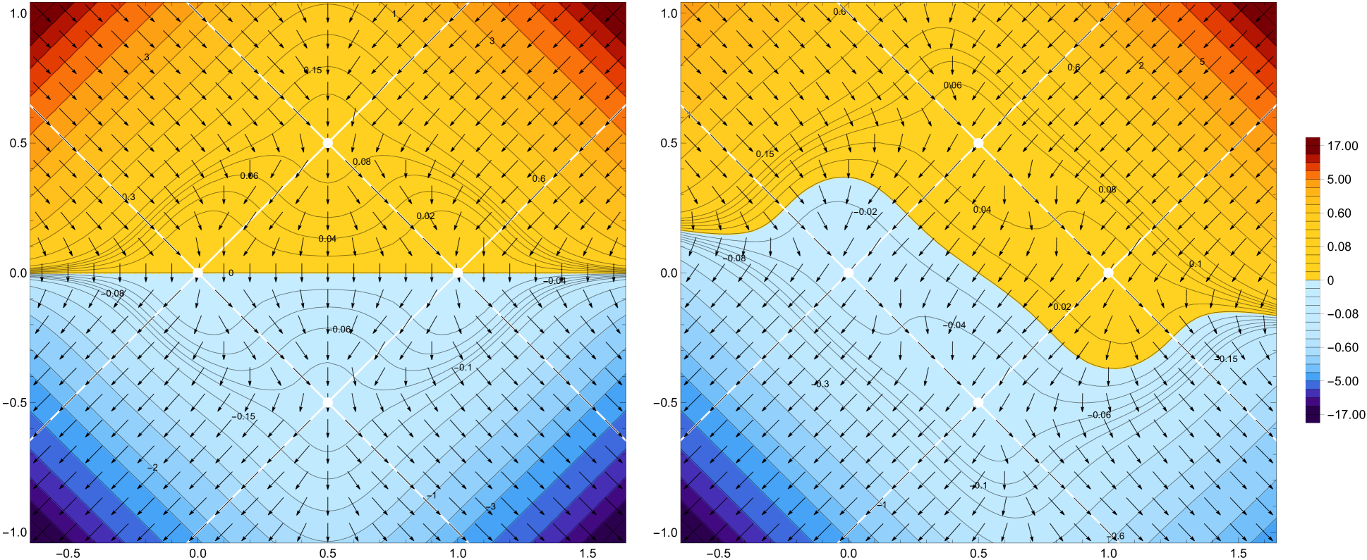
Figure 5: Vector fields for the mean values of the energy density currents (5.26) and (5.27), whose potential is the first expressions in (5.38), for either equal (left panel) or different (right panel) chemical potentials, in the same setup of Fig. 3.

The planar vector fields $\boldsymbol{\mathcal{J}}(x,t)$ and $\boldsymbol{\widetilde{\mathcal{J}}}(x,t)$ are displayed in Fig. 5 and Fig. 6 for the choice parameters reported in the caption of Fig. 3. In particular, $\mu_{+}=\mu_{-}$ in the left panels, while $\mu_{+}\neq\mu_{-}$ in the right panels. These vector fields have the same isolated critical points which are given by the vertices of the diamond $\mathcal{D}_{A}$. All of them have multiplicity $2$ and Poincaré index $0$. By applying the Poincaré-Hopf theorem (see Sec. 5.1), we find consistency with the fact that these vector fields can me mapped (through the stereographic projection) to vector fields on the Riemann sphere which have a critical point of index $2$ at the north pole.

The fluxes of the vector fields $\boldsymbol{\mathcal{J}}(x,t)$ and $\boldsymbol{\widetilde{\mathcal{J}}}(x,t)$ through the straight white lines in Fig. 5 and Fig. 6 vanish. Indeed, the absolute value of the ratios of their components is equal to 1 along these lines. Unfortunately, this analytic result is not properly shown in Fig. 5 and Fig. 6 because of a graphical failure in the displaying of these vector fields around their critical points. Another similar failure occurs at the vertices of $\mathcal{D}_{A}$, where arrows are displayed, while they should not because they are critical points of the vector fields. These failures could be related to the multiplicity of the critical points; indeed they do not occur for the vector fields shown in Fig. 3 and Fig. 4, whose critical points have multiplicity 1.

The local conductivities corresponding to (5.26)-(5.27) and (5.30)-(5.31) are respectively

$$\boldsymbol{\sigma}_{\mathcal{J}\!,e} \equiv \partial_{\mu_{e}}\boldsymbol{\mathcal{J}}(x,t)=-\frac{\kappa}{4\pi}\,\Big{(}\mu_{+}V(u_{+})^{2}-\mu_{-}V(u_{-})^{2}\,,\,\mu_{+}V(u_{+})^{2}+\mu_{-}V(u_{-})^{2}\Big{)}\hskip 22.76228pt$$ (5.32)

$$\rule{0.0pt}{19.91684pt}\boldsymbol{\sigma}_{\mathcal{J}\!,h} \equiv \partial_{\mu_{h}}\boldsymbol{\mathcal{J}}(x,t)=-\frac{\kappa}{4\pi}\,\Big{(}\mu_{+}V(u_{+})^{2}+\mu_{-}V(u_{-})^{2}\,,\,\mu_{+}V(u_{+})^{2}-\mu_{-}V(u_{-})^{2}\Big{)}$$ (5.33)

and

$$\boldsymbol{\sigma}_{\widetilde{\mathcal{J}}\!,e}\equiv\partial_{\mu_{e}}\boldsymbol{\widetilde{\mathcal{J}}}(x,t)=\boldsymbol{\sigma}_{\mathcal{J}\!,h}\;\;\;\qquad\;\;\;\boldsymbol{\sigma}_{\widetilde{\mathcal{J}}\!,h}\equiv\partial_{\mu_{h}}\boldsymbol{\widetilde{\mathcal{J}}}(x,t)=\boldsymbol{\sigma}_{\mathcal{J}\!,e}$$ (5.34)

which are independent of $\tau$; hence their Fourier transform gives only a Dirac delta term.

The ballistic nature of the modular transport observed through (5.9) is confirmed by the linear growth in $\tau$ of the following quantities

$$\int_{0}^{\tau}\boldsymbol{\mathcal{J}}(x,t)\,{\rm d}\tilde{\tau}=\boldsymbol{\mathcal{J}}(x,t)\,\tau\;\;\;\qquad\;\;\;\int_{0}^{\tau}\boldsymbol{\widetilde{\mathcal{J}}}(x,t)\,{\rm d}\tilde{\tau}=\boldsymbol{\widetilde{\mathcal{J}}}(x,t)\,\tau\,.$$ (5.35)

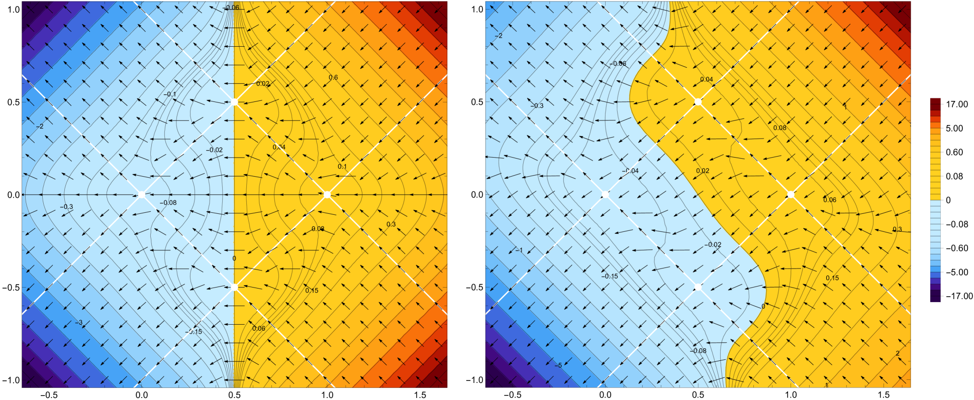
Figure 6: Vector fields for the mean values of the momentum density currents (5.30) and (5.31), whose potential is the second expressions in (5.38), for either equal (left panel) or different (right panel) chemical potentials, in the same setup of Fig. 3.

Both the vector fields defined by the energy and momentum currents are curl free and can be written as the gradient some potentials as follows

$$\langle\mathcal{J}_{x}(\tau;x,t)\rangle_{\mu}=-\,\partial_{x}\mathsf{W}_{\mathcal{J}}(x,t)\;\;\;\qquad\;\;\;\langle\mathcal{J}_{t}(\tau;x,t)\rangle_{\mu}=-\,\partial_{t}\mathsf{W}_{\mathcal{J}}(x,t)$$ (5.36)

and

$$\langle\widetilde{\mathcal{J}}_{x}(\tau;x,t)\rangle_{\mu}=-\,\partial_{x}\mathsf{W}_{\widetilde{\mathcal{J}}}(x,t)\;\;\;\qquad\;\;\;\langle\widetilde{\mathcal{J}}_{t}(\tau;x,t)\rangle_{\mu}=-\,\partial_{t}\mathsf{W}_{\widetilde{\mathcal{J}}}(x,t)$$ (5.37)

For the potentials $\mathsf{W}_{\mathcal{J}}$ and $\mathsf{W}_{\widetilde{\mathcal{J}}}$, we find respectively

$$\mathsf{W}_{\mathcal{J}}(x,t)\equiv\frac{\kappa}{4\pi}\big{[}\mu_{+}^{2}G(u_{+})-\mu_{-}^{2}G(u_{-})\big{]}\;\qquad\;\mathsf{W}_{\widetilde{\mathcal{J}}}(x,t)\equiv\frac{\kappa}{4\pi}\big{[}\mu_{+}^{2}G(u_{+})+\mu_{-}^{2}G(u_{-})\big{]}$$ (5.38)

being $G(u)$ defined as

$$G(u) \equiv \frac{2\pi^{2}}{15\,(b-a)^{2}}\left(u-\frac{a+b}{2}\right)\Big{[}\,6\,u^{4}-12(a+b)\,u^{3}+4\big{(}a^{2}+7ab+b^{2}\big{)}\,u^{2}$$

$$\hskip 99.58464pt+\,2\big{(}a^{3}-7a^{2}b-7ab^{2}+b^{3}\big{)}\,u+a^{4}-6a^{3}b+16a^{2}b^{2}-6ab^{3}+b^{4}\,\Big{]}$$

whose additive constant has been fixed by imposing the condition $G(\tfrac{a+b}{2})=0$. The expressions (5.26)-(5.27), (5.30)-(5.31), (5.36) and (5.37) are consistent because (5.2) and (4.7) are related as follows

$$\partial_{u}G(u)=V(u)^{2}\,.$$ (5.40)

Finally, since the vector fields $\boldsymbol{\mathcal{J}}(x,t)$ and $\boldsymbol{\widetilde{\mathcal{J}}}(x,t)$ are curl free, their line integrals along a curve depend only on the endpoints of the curve. Let us consider the curves anchored to the opposite vertices of $\mathcal{D}_{A}$, as done in Sec. 5.1. By employing (5.36) and (5.37), we find

$$\mathcal{L}[\boldsymbol{\mathcal{J}}]\big{(}\gamma(P_{a}\to P_{b})\big{)} = \mathsf{W}_{\mathcal{J}}\big{|}_{P_{a}}-\mathsf{W}_{\mathcal{J}}\big{|}_{P_{b}}\,=\,-\frac{4\pi}{5}\,\widetilde{\mathsf{E}}_{A}\hskip 39.83368pt$$ (5.41)

$$\rule{0.0pt}{17.07182pt}\mathcal{L}[\boldsymbol{\mathcal{J}}]\big{(}\gamma(P_{-\infty}\to P_{+\infty})\big{)} = \mathsf{W}_{\mathcal{J}}\big{|}_{P_{-\infty}}-\mathsf{W}_{\mathcal{J}}\big{|}_{P_{+\infty}}\,=\,-\frac{4\pi}{5}\,\mathsf{E}_{A}\hskip 28.45274pt$$ (5.42)

and

$$\mathcal{L}[\boldsymbol{\widetilde{\mathcal{J}}}]\big{(}\gamma(P_{a}\to P_{b})\big{)} = \mathsf{W}_{\widetilde{\mathcal{J}}}\big{|}_{P_{a}}-\mathsf{W}_{\widetilde{\mathcal{J}}}\big{|}_{P_{b}}\,=\,-\frac{4\pi}{5}\,\mathsf{E}_{A}\hskip 39.83368pt$$ (5.43)

$$\rule{0.0pt}{17.07182pt}\mathcal{L}[\boldsymbol{\widetilde{\mathcal{J}}}]\big{(}\gamma(P_{-\infty}\to P_{+\infty})\big{)} = \mathsf{W}_{\widetilde{\mathcal{J}}}\big{|}_{P_{-\infty}}-\mathsf{W}_{\widetilde{\mathcal{J}}}\big{|}_{P_{+\infty}}\,=\,-\frac{4\pi}{5}\,\widetilde{\mathsf{E}}_{A}\hskip 28.45274pt$$ (5.44)

where we have introduced

$$\mathsf{E}_{A}\equiv\frac{\kappa}{24}\big{(}\mu_{+}^{2}+\mu_{-}^{2}\big{)}\,\ell^{3}\;\;\;\qquad\;\;\;\widetilde{\mathsf{E}}_{A}\equiv\frac{\kappa}{24}\big{(}\mu_{+}^{2}-\mu_{-}^{2}\big{)}\,\ell^{3}$$ (5.45)

which correspond respectively to the mean value of the total energy (3.32) and of the total momentum (3.39) in the diamond $\mathcal{D}_{A}$ in the case where $f_{+}(u_{+})=f_{-}(u_{-})=0$ are imposed. Instead, from (4.6) we have that the mean values of (3.32) and (3.39) are $\langle E_{A}\rangle_{\mu}=\langle\widetilde{E}_{A}\rangle_{\mu}=0$.

The vanishing of the line integrals in (5.42) and (5.44) for $\mu_{+}=\mu_{-}$ can be observed also from the left panel of Fig. 5 and Fig. 6 respectively.

We find it worth considering also the fluxes of $\boldsymbol{\mathcal{J}}(x,t)$ and $\boldsymbol{\widetilde{\mathcal{J}}}(x,t)$ through the curves $\gamma_{t_{0}}$ and $\gamma_{x_{0}}$ introduced in Sec. 5.1. They can be written as

$$\mathcal{F}[\boldsymbol{\mathcal{J}}]\big{(}\gamma_{t_{0}}(P_{a}\to P_{b})\big{)} = -\frac{4\pi}{5}\,\mathsf{E}_{A}\,F(2t_{0}/\ell)$$ (5.46)

$$\rule{0.0pt}{17.07182pt}\mathcal{F}[\boldsymbol{\mathcal{J}}]\big{(}\gamma_{x_{0}}(P_{-\infty}\to P_{+\infty})\big{)} = -\frac{4\pi}{5}\,\widetilde{\mathsf{E}}_{A}\,F\big{(}2(x_{0}-\tfrac{a+b}{2})/\ell\big{)}$$ (5.47)

and

$$\mathcal{F}[\boldsymbol{\widetilde{\mathcal{J}}}]\big{(}\gamma_{t_{0}}(P_{a}\to P_{b})\big{)} = -\frac{4\pi}{5}\,\widetilde{\mathsf{E}}_{A}\,F(2t_{0}/\ell)$$ (5.48)

$$\rule{0.0pt}{17.07182pt}\mathcal{F}[\boldsymbol{\widetilde{\mathcal{J}}}]\big{(}\gamma_{x_{0}}(P_{-\infty}\to P_{+\infty})\big{)} = -\frac{4\pi}{5}\,\mathsf{E}_{A}\,F\big{(}2(x_{0}-\tfrac{a+b}{2})/\ell\big{)}$$ (5.49)

in terms of the mean values of total charges (5.45), where $F(y)$ is defined for $|y|<1$ as follows

$$F(y)\equiv\frac{5\left(1-y^{2}\right)^{2}}{64\,y^{5}}\left[\,2y\big{(}3y^{4}-2y^{2}+3\big{)}-3\left(1-y^{2}\right)^{2}\left(1+y^{2}\right)\log\!\left(\frac{1+y}{1-y}\right)\right].$$ (5.50)

This function is even, vanishes as $|y|\to 1$ and takes its maximum value equal to $1$ at $y=0$.

5.3 Quantum noise

Quantum effects along the conventional temporal evolution of any observable $\mathcal{O}$ generate non-trivial fluctuations around its mean value $\langle\mathcal{O}\rangle$. This is the case for the modular evolution as well. For instance, the quadratic fluctuations of the current $j_{x}(\tau;x,t)$ describe the quantum noise produced by the transport of charged particles. It is known [45, 46] that, besides spoiling the charge propagation and detection, the noise carries also useful information because it provides the experimental basis of noise spectroscopy.

The basic quantity of interest is the (modular) noise power generated by the charge current (3.6) at frequency $\omega$ in the point $(x,t)$ of the spacetime, defined as follows

$$P_{j}(\omega;x,t)\,\equiv\,-\int_{-\infty}^{\infty}\langle j_{x}(\tau_{1};x,t)\,j_{x}(\tau_{2};x,t)\rangle_{\mu}^{\textrm{\tiny con}}\;{\rm e}^{{\rm i}\omega\tau_{12}}\,{\rm d}\tau_{12}\,.$$ (5.51)

Since $\tau_{12}$ is dimensionless, the corresponding frequency $\omega$ is dimensionless as well. Notice that the noise power is generated only by $j_{x}$ because $\langle j_{t}(\tau_{1};x,t)\,j_{t}(\tau_{2};x,t)\rangle_{\mu}^{\textrm{\tiny con}}$ vanishes identically. Indeed, $j_{t}$ introduced in (3.9) is proportional to the identity operator, being generated only by the central extension $\kappa$ in the r.h.s. of (2.5).

Considering (3.13), we remark that $\langle j_{x}(\tau_{1};x,t)\,j_{x}(\tau_{2};x,t)\rangle_{\mu}^{\textrm{\tiny con}}=\langle\hat{j}_{x}(\tau_{1};x,t)\,\hat{j}_{x}(\tau_{2};x,t)\rangle_{\mu}^{\textrm{\tiny con}}$; indeed $j_{x}(\tau;x,t)$ and $\hat{j}_{x}(\tau;x,t)$ differ by a real function.

By using (3.6), the modular noise power can be expressed in terms of the two-point functions of the chiral currents $j_{\pm}(\tau,u)$

$$P_{j}(\omega;x,t) = -\int_{-\infty}^{\infty}\Big{[}\,V(u_{+})^{2}\,\langle j_{+}(\tau_{1},u_{+})\,j_{+}(\tau_{2},u_{+})\rangle_{\mu_{+}}^{\textrm{\tiny con}}$$

$$\hskip 42.67912pt+\,V(u_{-})^{2}\,\langle j_{-}(\tau_{1},u_{-})\,j_{-}(\tau_{2},u_{-})\rangle_{\mu_{-}}^{\textrm{\tiny con}}\,\Big{]}{\rm e}^{{\rm i}\omega\tau_{12}}\,{\rm d}\tau_{12}\,.$$

By employing (4.4) and the limit given in (4.50), we have that the dependence on $V(u_{+})$ and $V(u_{-})$ drops out and therefore (5.3) becomes (see (F.3) for the evaluation of the integral)

$$P_{j}(\omega;x,t) = -\frac{\kappa}{4}\,\lim_{\varepsilon\to 0}\,\int_{-\infty}^{\infty}\left[\,\frac{1}{\sinh^{2}(\pi\tau-{\rm i}\varepsilon)}+\frac{1}{\sinh^{2}(-\pi\tau+{\rm i}\varepsilon)}\,\right]{\rm e}^{{\rm i}\omega\tau}\,{\rm d}\tau$$

$$= -\frac{\kappa}{2}\,\lim_{\varepsilon\to 0}\,\int_{-\infty}^{\infty}\frac{{\rm e}^{{\rm i}\omega\tau}}{\sinh^{2}(\pi\tau-{\rm i}\varepsilon)}\,{\rm d}\tau\,=\,\frac{\kappa}{2\pi}\;\omega\coth(\omega/2)+\frac{\kappa}{2\pi}\,\omega$$ (5.53)

which is indepedent of $x$ and $t$. The zero frequency limit of (5.53) reads

$$P_{j}(0;x,t)=\lim_{\omega\to 0}P_{j}(\omega;x,t)=\frac{\kappa}{\pi}\;.$$ (5.54)

It is worth comparing this result with the Johnson-Nyquist law [47, 48]. In a CFT on the line at finite inverse temperature $\beta$ and vanishing chemical potential, the two-point functions of the chiral currents read

$$\langle j_{\pm}(u)\,j_{\pm}(v)\rangle_{{}_{\textrm{\tiny$\beta$}}}^{\textrm{\tiny con}}=\frac{\kappa}{4\pi^{2}}\bigg{(}\frac{\pi}{\beta\,\sinh\!\big{[}\pi(u-v\mp{\rm i}\varepsilon)/\beta\big{]}}\bigg{)}^{2}.$$ (5.55)

Since $\varrho(x,t)=j_{+}(u_{+})+j_{-}(u_{-})$, $j_{x}(x,t)=j_{+}(u_{+})-j_{-}(u_{-})$ and $\langle j_{\pm}(u)\,j_{\mp}(v)\rangle_{{}_{\textrm{\tiny$\beta$}}}^{\textrm{\tiny con}}=0$, by using (F.3) the noise power $P_{\textrm{\tiny JN}}(\omega)$ at frequency $\omega$ in the point $x$ of the space for $\varrho$ and $j_{x}$ coincide and read

$$P_{\textrm{\tiny JN}}(\omega) \equiv -\int_{-\infty}^{\infty}\!\langle\varrho(x,t_{1})\,\varrho(x,t_{2})\rangle_{\beta}^{\textrm{\tiny con}}\;{\rm e}^{{\rm i}\omega t_{12}}\,{\rm d}t_{12}\,=\,-\int_{-\infty}^{\infty}\!\langle j_{x}(x,t_{1})\,j_{x}(x,t_{2})\rangle_{\beta}^{\textrm{\tiny con}}\;{\rm e}^{{\rm i}\omega t_{12}}\,{\rm d}t_{12}$$

$$= -\frac{\kappa}{4\,\beta^{2}}\,\lim_{\varepsilon\to 0}\,\int_{-\infty}^{\infty}\bigg{(}\,\frac{1}{\sinh^{2}\!\big{[}\pi(t-{\rm i}\varepsilon)/\beta\big{]}}+\frac{1}{\sinh^{2}\!\big{[}\pi(-t+{\rm i}\varepsilon)/\beta\big{]}}\,\bigg{)}\,{\rm e}^{{\rm i}\omega t}\,{\rm d}t\hskip 28.45274pt$$

$$= -\frac{\kappa}{2\,\beta^{2}}\,\lim_{\varepsilon\to 0}\,\int_{-\infty}^{\infty}\frac{{\rm e}^{{\rm i}\omega t}}{\sinh^{2}\!\big{[}\pi(t-{\rm i}\varepsilon)/\beta\big{]}}\,{\rm d}t\,=\,\frac{\kappa}{2\pi}\;\omega\coth(\beta\omega/2)+\frac{\kappa}{2\pi}\,\omega$$ (5.56)

which is independent of $x$ because of the translation invariance of the CFT. The zero frequency limit of (5.56) gives the Johnson-Nyquist law

$$P_{\textrm{\tiny JN}}(0)=\frac{\kappa}{\pi\beta}$$ (5.57)

Comparing (5.53) with (5.56) and also the corresponding zero frequency limits given by (5.54) with (5.57) confirms that the modular evolution has a thermal character with inverse temperature $\tilde{\beta}=1$, which appears in the KMS condition (4.49) satisfied by the modular correlation functions (4.4), (4.43), (4.4) and (4.4). We remark that the noise power (5.54) provides a physical observable [45, 46] where in principle the modular temperature can be measured.

We can also introduce the modular noise power $P_{k}(\omega;x,t)$ at frequency $\omega$ in the point $(x,t)$ of the spacetime generated by the helicity current (3.22), defined by the r.h.s. (5.51) with $j_{x}$ replaced by $k_{x}$. From the explicit expression of $\langle k_{x}(\tau_{1};x,t)\,k_{x}(\tau_{2};x,t)\rangle_{\mu}^{\textrm{\tiny con}}$ and (C.14)-(C.15), it is straightforward to obtain the r.h.s. of (5.3) for $P_{k}(\omega;x,t)$; hence $P_{j}(\omega;x,t)=P_{k}(\omega;x,t)$. Indeed, the differences due to the diverse relative signs in (3.6) and (3.21) do not lead to a relevant result in this computation because the mixed connected correlators vanish.

Similarly, it is worth investigating the noise generated by the energy current (3.29), namely

$${\cal P_{J}}(\omega;x,t)\equiv\int_{-\infty}^{\infty}\!\langle\mathcal{J}_{x}(\tau_{1};x,t)\,\mathcal{J}_{x}(\tau_{2};x,t)\rangle_{\mu}^{\textrm{\tiny con}}\;{\rm e}^{{\rm i}\omega\tau_{12}}\,{\rm d}\tau_{12}\,.$$ (5.58)

From (4.4) and the identity (4.50), one finds (see (F.5) for the evaluation of the integral)

$${\cal P_{J}}(\omega;x,t) = \frac{\pi^{2}c}{8}\,\lim_{\varepsilon\to 0}\,\int_{-\infty}^{\infty}\left[\,\frac{1}{\sinh^{4}(\pi\tau-{\rm i}\varepsilon)}+\frac{1}{\sinh^{4}(-\pi\tau+{\rm i}\varepsilon)}\,\right]{\rm e}^{{\rm i}\omega\tau}\,{\rm d}\tau$$ (5.59)

$$= \frac{\pi^{2}c}{4}\,\lim_{\varepsilon\to 0}\,\int_{-\infty}^{\infty}\frac{{\rm e}^{{\rm i}\omega\tau}}{\sinh^{4}(\pi\tau-{\rm i}\varepsilon)}\,{\rm d}\tau\,=\frac{c}{24\pi}\,\big{(}4\pi^{2}+\omega^{2}\big{)}\,\big{[}\,\omega\coth(\omega/2)+\omega\,\big{]}\hskip 28.45274pt$$ (5.60)

which is indepedent of $x$ and $t$, and whose zero frequency limit gives

$${\cal P_{J}}(0;x,t)=\lim_{\omega\to 0}{\cal P_{J}}(\omega;x,t)=\frac{\pi\,c}{3}\;.$$ (5.61)

It is worth comparing these results based on the modular evolution with the corresponding ones based on the standard temporal evolution. In a CFT on the line at finite temperature and vanishing chemical potential, we have

$$\langle T_{\pm}(u)\,T_{\pm}(v)\rangle_{{}_{\textrm{\tiny$\beta$}}}^{\textrm{\tiny con}}=\frac{c}{8\pi^{2}}\bigg{(}\frac{\pi}{\beta\,\sinh\!\big{[}\pi(u-v\mp{\rm i}\varepsilon)/\beta\big{]}}\bigg{)}^{4}.$$ (5.62)

Since $T_{tt}(x,t)=T_{+}(u_{+})+T_{-}(u_{-})$, $T_{xt}(x,t)=T_{+}(u_{+})-T_{-}(u_{-})$ and $\langle T_{\pm}(u)\,T_{\mp}(v)\rangle_{{}_{\textrm{\tiny$\beta$}}}^{\textrm{\tiny con}}=0$, the noise power $\mathcal{P}_{\textrm{\tiny JN}}(\omega)$ at frequency $\omega$ in the point $x$ of the space of $T_{tt}$ and $T_{xt}$ coincide. It reads

$$\mathcal{P}_{\textrm{\tiny JN}}(\omega) \equiv \int_{-\infty}^{\infty}\!\langle T_{xt}(x,t_{1})\,T_{xt}(x,t_{2})\rangle_{\beta}^{\textrm{\tiny con}}\;{\rm e}^{{\rm i}\omega t_{12}}\,{\rm d}t_{12}\,=\,\int_{-\infty}^{\infty}\!\langle T_{tt}(x,t_{1})\,T_{tt}(x,t_{2})\rangle_{\beta}^{\textrm{\tiny con}}\;{\rm e}^{{\rm i}\omega t_{12}}\,{\rm d}t_{12}$$

$$= \frac{\pi^{2}c}{8\,\beta^{4}}\,\lim_{\varepsilon\to 0}\,\int_{-\infty}^{\infty}\bigg{(}\,\frac{1}{\sinh^{4}\!\big{[}\pi(t-{\rm i}\varepsilon)/\beta\big{]}}+\frac{1}{\sinh^{4}\!\big{[}\pi(-t+{\rm i}\varepsilon)/\beta\big{]}}\,\bigg{)}\,{\rm e}^{{\rm i}\omega t}\,{\rm d}t\hskip 28.45274pt$$ (5.63)

$$= \frac{\pi^{2}c}{4\,\beta^{4}}\,\lim_{\varepsilon\to 0}\,\int_{-\infty}^{\infty}\frac{{\rm e}^{{\rm i}\omega t}}{\sinh^{4}\!\big{[}\pi(t-{\rm i}\varepsilon)/\beta\big{]}}\,{\rm d}t$$ (5.64)

$$= \frac{c}{24\pi\,\beta^{2}}\,\big{[}\,4\pi^{2}+(\beta\omega)^{2}\,\big{]}\,\big{[}\,\omega\coth(\beta\omega/2)+\omega\,\big{]}$$ (5.65)

where (F.5) has been employed and whose zero frequency limit is

$$\mathcal{P}_{\textrm{\tiny JN}}(0)=\frac{\pi\,c}{3\,\beta^{3}}\,.$$ (5.66)

Comparing (5.65) with the modular noise (5.60) provides another consistency check for the fact that the modular evolution has a thermal character with inverse temperature $\tilde{\beta}=1$.

Thus, while $P_{j}(0;x,t)$ provides the coefficient $\kappa$ of the central term in (2.5) through (5.54), ${\cal P_{J}}(0;x,t)$ gives the central charge $c$ through (5.61). Notice that in the derivation of (5.60), the expression (4.37) has been employed, which holds for the specific velocity given in (4.7).

The noise ${\cal P}_{\widetilde{\mathcal{J}}}(\omega;x,t)$ generated by the momentum current (3.37) is defined by the r.h.s. of (5.58) with $\mathcal{J}_{x}$ replaced by $\widetilde{\mathcal{J}}_{x}$. By adapting the observations made above to get $P_{j}(\omega;x,t)=P_{k}(\omega;x,t)$ and using (C)-(C), one finds that ${\cal P}_{\widetilde{\mathcal{J}}}(\omega;x,t)={\cal P}_{\mathcal{J}}(\omega;x,t)$.

The previous analysis shows that the modular noise power generated by the charge and energy currents is uniform in space and time, despite the fact that the translation invariance is broken by the bipartition of the system. This peculiar feature does not hold for the quadratic fluctuations of a generic observable. Indeed, consider for instance the modular noise power relative to the charge density (3.4), namely

$$P_{\varrho}(\omega;x,t)\,\equiv\,-\int_{-\infty}^{\infty}\!\langle\varrho(\tau_{1};x,t)\,\varrho(\tau_{2};x,t)\rangle_{\mu}^{\textrm{\tiny con}}\;{\rm e}^{{\rm i}\omega\tau_{12}}\,{\rm d}\tau_{12}\,.$$ (5.67)

By using (4.4), (4.50) and (F.3), we find

$$P_{\varrho}(\omega;x,t) = -\frac{\kappa}{4}\,\lim_{\varepsilon\to 0}\,\int_{-\infty}^{\infty}\left[\,\frac{1}{V(u_{+})^{2}\,\sinh^{2}(\pi\tau-{\rm i}\varepsilon)}+\frac{1}{V(u_{-})^{2}\,\sinh^{2}(-\pi\tau+{\rm i}\varepsilon)}\,\right]{\rm e}^{{\rm i}\omega\tau}\,{\rm d}\tau$$

$$= -\frac{\kappa}{4}\left[\frac{1}{V^{2}(u_{+})}+\frac{1}{V^{2}(u_{-})}\right]\lim_{\varepsilon\to 0}\,\int_{-\infty}^{\infty}\frac{{\rm e}^{{\rm i}\omega\tau}}{\sinh^{2}(\pi\tau-{\rm i}\varepsilon)}\,{\rm d}\tau$$

$$= \frac{\kappa}{4\pi}\left[\,\frac{1}{V^{2}(u_{+})}+\frac{1}{V^{2}(u_{-})}\,\right]\big{[}\,\omega\coth(\omega/2)+\omega\,\big{]}$$ (5.68)

that depends on the frequency and on the position in spacetime. The zero frequency limit of (5.68) gives

$$P_{\varrho}(0;x,t)=\frac{\kappa}{2\pi}\left[\frac{1}{V(u_{+})^{2}}+\frac{1}{V(u_{-})^{2}}\right]$$ (5.69)

which is qualitatively different from (5.54) because of the occurrence of a non trivial dependence on the spacetime position. Notice that, setting $V(u)=1$ identically in (5.69) one recovers (5.57) in the special case of $\beta=1$.

We can introduce also the noise $P_{\chi}(\omega;x,t)$ generated by $\chi$ in (3.19) as the Fourier transform in $\tau_{12}$ of the connected modular two-point function of $\chi$ at coincident points, as done in (5.67) for $P_{\varrho}(\omega;x,t)$. Comparing this computation with the one reported above for $P_{\varrho}(\omega;x,t)$, we observe again that the differences due to the different relative sign in (3.4) and (3.19) do not play any role because the mixed connected correlators vanish; hence $P_{\chi}(\omega;x,t)=P_{\varrho}(\omega;x,t)$.

We can perform a non trivial consistency check of the above results by considering the Fourier transform of the anticommutator

$$\mathcal{A}[\mathcal{O}](\omega;x,t)\,\equiv\,\frac{1}{2}\int_{-\infty}^{\infty}\langle\,\big{\{}\,\mathcal{O}(\tau_{1};x,t)\,,\mathcal{O}(\tau_{2};x,t)\,\big{\}}\,\rangle_{\mu}^{\textrm{\tiny con}}\,{\rm e}^{{\rm i}\omega\tau_{12}}\,{\rm d}\tau_{12}$$ (5.70)

and the Fourier transform of the commutator

$$\rule{0.0pt}{19.91684pt}\mathcal{C}[\mathcal{O}](\omega;x,t)\,\equiv\,\frac{1}{2}\int_{-\infty}^{\infty}\langle\,\big{[}\,\mathcal{O}(\tau_{1};x,t)\,,\mathcal{O}(\tau_{2};x,t)\,\big{]}\,\rangle_{\mu}^{\textrm{\tiny con}}\,{\rm e}^{{\rm i}\omega\tau_{12}}\,{\rm d}\tau_{12}$$ (5.71)

for the modular correlators of the operators $\mathcal{O}\in\big{\{}j_{x},k_{x},\mathcal{J}_{x},\widetilde{\mathcal{J}}_{x},\rho,\chi\big{\}}$ considered above. Since the Fourier transform $F(\omega)\equiv\int_{-\infty}^{+\infty}f(t)\,{\rm e}^{{\rm i}\omega t}{\rm d}t$ of a generic function $f(t)$ satisfies the property $\tfrac{1}{2}\int_{-\infty}^{+\infty}\!\big{[}f(t)\pm f(-t)\big{]}{\rm e}^{{\rm i}\omega t}{\rm d}t=\tfrac{1}{2}\big{[}F(\omega)\pm F(-\omega)\big{]}$, by employing (5.53), (5.60) and (5.68), for (5.70) and (5.71) we find that the following modular fluctuation-dissipation relation

$$\mathcal{A}[\mathcal{O}](\omega;x,t)\,=\,\coth\!\left(\frac{\omega}{2}\right)\,\mathcal{C}[\mathcal{O}](\omega;x,t)$$ (5.72)

which corresponds to the fluctuation-dissipation relation [49, 50, 51] with inverse temperature given by $\tilde{\beta}=1$. In the case of two-dimensional CFT, this result further confirms the thermal nature of the modular evolution with inverse temperature $\tilde{\beta}=1$, in agreement with the KMS condition discussed in Sec. 4.4.

6 Finite volume

In this section the analyses of Sec. 4 are extended to a two-dimensional CFT at finite density and finite volume by compactifying each chiral direction on the circle of length $L$, hence the resulting spacetime $\mathbb{M}_{\diamond}$ has the topology of the torus. In Sec. 6.1 the relevant chiral correlators are discussed. The modular Hamiltonian associated to the bipartition of each chiral direction provided by the interval $A=[a,b]$ and the corresponding modular correlators are explored in Sec. 6.2 and Sec. 6.3 respectively.

6.1 Finite density representation on the circle

The finite density and finite volume representation of a CFT on a circle of length $L$ can be obtained from its ground state representation in the infinite line, by employing first the conformal transformation $u\mapsto{\rm e}^{2\pi{\rm i}u/L}$ and then the automorphism described in the Appendix C.

In this representation, the one-point functions are obtained by first applying the conformal transformation $u\mapsto{\rm e}^{2\pi{\rm i}u/L}$ to the one-point functions in the ground state and on the line, which are given by (4.1) with $\mu_{+}=\mu_{-}=0$, and then employing the automorphism discussed in the Appendix C. The result is

$$\langle\phi_{\pm}(u)\rangle_{{}_{\textrm{\tiny$L,\mu_{\pm}$}}}\!=\,0\;\;\qquad\;\;\langle j_{\pm}(u)\rangle_{{}_{\textrm{\tiny$L,\mu_{\pm}$}}}\!=\,-\frac{\kappa\mu_{\pm}}{2\pi}\;\;\qquad\;\;\langle{\cal T}_{\pm}(u)\rangle_{{}_{\textrm{\tiny$L,\mu_{\pm}$}}}\!=\,\frac{\kappa\mu^{2}_{\pm}}{4\pi}-\frac{\pi c}{12L^{2}}\;\;$$ (6.1)

where we used that the Schwarzian derivative (2.35) of the conformal map $u\mapsto{\rm e}^{2\pi{\rm i}u/L}$ is equal to $2\pi^{2}/L^{2}$. In the infinite volume limit $L\to+\infty$, the one-point functions (6.1) become the ones in (4.1), as expected.

The connected two-point functions in the finite density and finite volume representation can be written through the same procedure, starting from the connected two-point functions in the ground state representation. From (4.2), for the connected two-point expectation values of $\phi_{\pm}$ we obtain

$$\langle\phi_{\pm}^{*}(u)\,\phi_{\pm}(v)\rangle_{{}_{\textrm{\tiny$L,\mu_{\pm}$}}}^{\textrm{\tiny con}}\!=\frac{{\rm e}^{\pm{\rm i}\mu_{\pm}(u-v)}}{2\pi\,{\rm e}^{\pm{\rm i}\pi h_{\pm}}}\bigg{(}\frac{\pi}{L\,\sin\!\big{[}\pi(u-v\mp{\rm i}\varepsilon)/L\big{]}}\bigg{)}^{2h_{\pm}}\;\;\qquad\;\;\frac{L\mu_{\pm}}{2\pi}\in\mathbb{Z}$$ (6.2)

whose r.h.s. is periodic, as expected. In the Appendix D.1, a consistency check of (6.2) is discussed by considering the special case of a free fermion with anti-periodic boundary conditions and obtaining the corresponding two-point function through the Fermi-Dirac distribution.
As for the two-point functions of $j_{\pm}$ and ${\cal T}_{\pm}$, from (4.3) and (4.4) we find respectively

$$\langle j_{\pm}(u)\,j_{\pm}(v)\rangle_{{}_{\textrm{\tiny$L,\mu_{\pm}$}}}^{\textrm{\tiny con}}=\frac{\kappa}{4\pi^{2}}\bigg{(}\frac{\pi}{L\,\sin\!\big{[}\pi(u-v\mp{\rm i}\varepsilon)/L\big{]}}\bigg{)}^{2}$$ (6.3)

and

$$\langle{\cal T}_{\pm}(u)\,{\cal T}_{\pm}(v)\rangle_{{}_{\textrm{\tiny$L,\mu_{\pm}$}}}^{\textrm{\tiny con}}=\frac{c}{8\pi^{2}}\bigg{(}\frac{\pi}{L\,\sin\!\big{[}\pi(u-v\mp{\rm i}\varepsilon)/L\big{]}}\bigg{)}^{4}\,.$$ (6.4)

We also have that

$$\langle{\cal T}_{\pm}(u)\,j_{\pm}(v)\rangle_{{}_{\textrm{\tiny$L,\mu_{\pm}$}}}^{\textrm{\tiny con}}=-\,\mu_{\pm}\,\langle j_{\pm}(u)\,j_{\pm}(v)\rangle_{{}_{\textrm{\tiny$L,\mu_{\pm}$}}}^{\textrm{\tiny con}}\,.$$ (6.5)

The connected mixed correlators involving fields having different chiralities vanish identically. Notice that the infinite volume limit $L\to+\infty$ of the two-point correlators (6.2), (6.3) and (6.4) gives the two-point correlators on line (4.2), (4.3) and (4.4) respectively, as expected.

6.2 Modular Hamiltonian and modular conjugation

In the following we consider the portion of Minkowski spacetime described by the light-cone coordinates $(u_{+},u_{-})$ when periodic boundary conditions are imposed along both the chiral directions with the same period equal to $L$. The resulting spacetime $\mathbb{M}_{\diamond}$ has the topology of a torus and it is shown is Fig. 7, where $u_{\pm}\in(-L/2\,,L/2)$ and the dashed segments having the same colour are identified. We consider a two-dimensional CFT in the finite density state on this spacetime. Moreover, each chiral direction is partitioned through the interval $A=[a,b]$ with length $\ell\equiv b-a$ and its complement; hence the diamond $\mathcal{D}_{A}$ can be introduced. The two panels of Fig. 7 describe the same setup in two equivalent ways and $\mathcal{D}_{A}$ corresponds to the grey region in each panel.

A standard way to compactify a chiral direction exploits the Cayley map, which relates the real line to the unit circle $\mathbb{S}$ with one point removed (see e.g. [52]) and reads $u\mapsto z=\tfrac{1+{\rm i}\,v}{1-{\rm i}\,v}$ where $v\in{\mathbb{R}}$ and $z\in\mathbb{S}\setminus\{P_{0}\}$, being $P_{0}$ the point at $\theta=\pi$ on $\mathbb{S}$. By employing the complex number $z={\rm e}^{2\pi{\rm i}u/L}$ with $u\sim u+L$ to parameterise $\mathbb{S}$, where $L$ corresponds to the compactification parameter, the Cayley map and its inverse read respectively

$${\rm e}^{2\pi{\rm i}u/L}=\frac{1+{\rm i}\,v}{1-{\rm i}\,v}\;\;\;\;\qquad\;\;\;\;v\,=\,{\rm i}\;\frac{1-{\rm e}^{2\pi{\rm i}u/L}}{1+{\rm e}^{2\pi{\rm i}u/L}}\,=\,\tan(\pi u/L)\,\equiv\,\mathcal{C}(u)\,.$$ (6.6)

Alternatively [53], one first introduces the periodic identification $u\sim u+L$ on the real line and then uses the exponential map $u\mapsto{\rm e}^{2\pi{\rm i}u/L}$.

By adapting the general results described in Sec. 2.2, in this CFT setup the modular Hamiltonian of $A$ and the corresponding full modular Hamiltonian read respectively [9, 10]

$$K_{A}=\int_{A}V_{L}(u_{+})\left[\,{\cal T}_{+}(u_{+})-\frac{\kappa\mu^{2}_{+}}{4\pi}+\frac{\pi c}{12L^{2}}\,\right]\!{\rm d}u_{+}+\int_{A}V_{L}(u_{-})\left[\,{\cal T}_{-}(u_{-})-\frac{\kappa\mu^{2}_{-}}{4\pi}+\frac{\pi c}{12L^{2}}\,\right]\!{\rm d}u_{-}$$ (6.7)

and

$$K\equiv K_{A}\otimes\boldsymbol{1}_{B}-\boldsymbol{1}_{A}\otimes K_{B} = \int_{-L/2}^{L/2}V_{L}(u_{+})\left[\,{\cal T}_{+}(u_{+})-\frac{\kappa\mu^{2}_{+}}{4\pi}+\frac{\pi c}{12L^{2}}\,\right]{\rm d}u_{+}$$

$$+\int_{-L/2}^{L/2}V_{L}(u_{-})\left[\,{\cal T}_{-}(u_{-})-\frac{\kappa\mu^{2}_{-}}{4\pi}+\frac{\pi c}{12L^{2}}\,\right]{\rm d}u_{-}$$ (6.8)

where the velocity $V_{L}(u)$ is

$$V_{L}(u)=2L\,\frac{\sin[\pi(b-u)/L]\,\sin[\pi(u-a)/L]}{\sin[\pi(b-a)/L]}=\frac{1}{w_{L}^{\prime}(u)}\;\;\;\qquad\;\;\;u\in A$$ (6.9)

being $w_{L}(u)$ defined as follows

$$w_{L}(u)\equiv\frac{1}{2\pi}\,\log\!\left(\!-\frac{\sin[\pi(u-a)/L]}{\sin[\pi(u-b)/L]}\right).$$ (6.10)

The weight function (6.9) can be obtained from (4.7) as follows

$$V_{L}(v)=\frac{\widetilde{V}\big{(}{\rm e}^{2\pi{\rm i}v/L}\big{)}}{\partial_{v}\big{(}{\rm e}^{2\pi{\rm i}v/L}\big{)}}=\frac{\widehat{V}\big{(}\mathcal{C}(v)\big{)}}{\mathcal{C}^{\prime}(v)}$$ (6.11)

where $\widetilde{V}(v)$ is defined as (4.7) with $a$ and $b$ replaced by ${\rm e}^{2\pi{\rm i}a/L}$ and ${\rm e}^{2\pi{\rm i}b/L}$ respectively, while in the last expression the Cayley map (6.6) is employed and $\widehat{V}(v)$ is given by (4.7) with $a$ and $b$ replaced by $\mathcal{C}(a)$ and $\mathcal{C}(b)$ respectively. The full modular Hamiltonian (6.2) corresponds (2.6) specialised to $V_{+}(u)=V_{-}(u)=V_{L}(u)$ given by (6.9), which vanishes only at the endpoints of $A$. Notice that a vanishing additive constant has been chosen in (6.7).

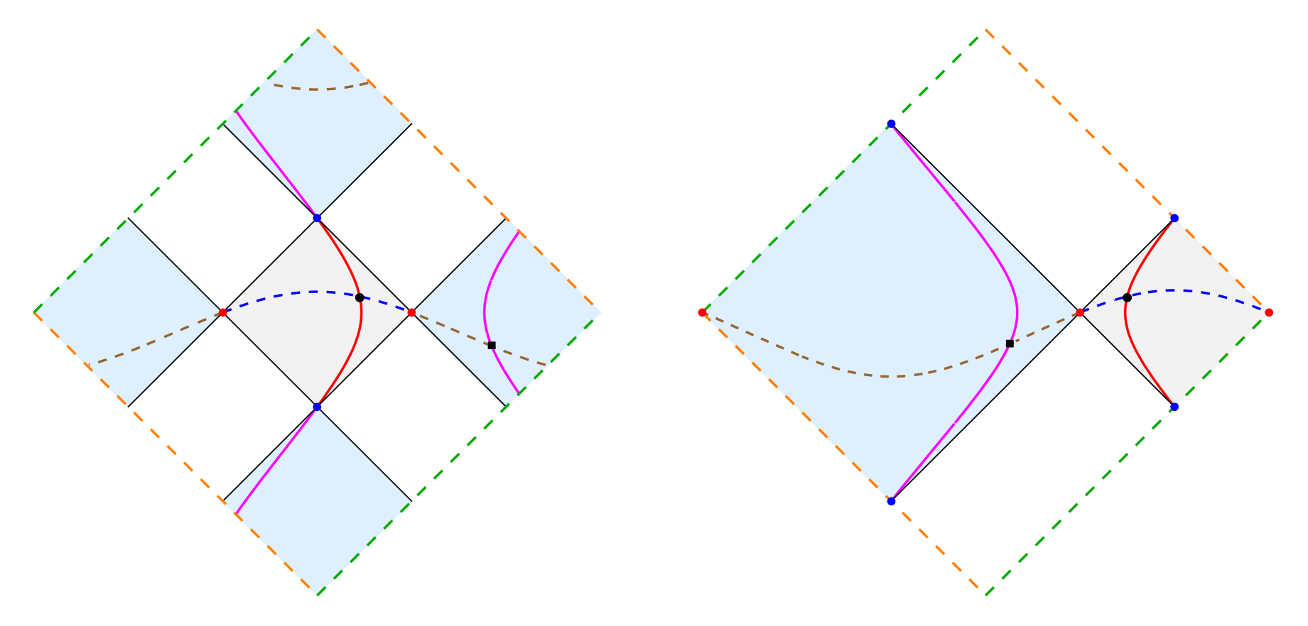
Figure 7: Modular trajectories generated either by the modular Hamiltonian (6.2) (solid lines) or by the modular momentum (dashed lines) for the CFT on the circle. Since periodic boundary conditions are imposed, the green (orange) dashed straight lines must be identified. The solid (dashed) curves having different colours are related through the geometric action of the modular conjugation, constructed from (6.18).

The modular evolution generated by (6.2) can be studied by applying the results discussed in Sec. 2.2 to $V_{+}(u)=V_{-}(u)=V_{L}(u)$ and $w_{+}(u)=w_{-}(u)=w_{L}(u)$, introduced in (6.9) and (6.10) respectively. In this case (2.16) becomes [54]

$$\xi_{\pm}(\tau,u)=\xi_{L}(\pm\tau,u)\;\;\;\qquad\;\;\;\xi_{L}(\tau,u)\equiv\frac{L}{2\pi\,{\rm i}}\,\log\!\bigg{(}\frac{{\rm e}^{\pi{\rm i}(b+a)/L}+{\rm e}^{2\pi{\rm i}b/L}\,{\rm e}^{2\pi w_{L}(u)+2\pi\tau}}{{\rm e}^{\pi{\rm i}(b-a)/L}+{\rm e}^{2\pi w_{L}(u)+2\pi\tau}}\bigg{)}$$ (6.12)

whose infinite volume limit $L\to+\infty$ gives (4.11), as expected. From (6.12) we have

$${\rm e}^{2\pi{\rm i}\xi_{L}(\tau,u)/L} = \frac{\big{(}{\rm e}^{2\pi{\rm i}b/L}-{\rm e}^{2\pi{\rm i}u/L}\big{)}\,{\rm e}^{2\pi{\rm i}a/L}+\big{(}{\rm e}^{2\pi{\rm i}u/L}-{\rm e}^{2\pi{\rm i}a/L}\big{)}\,{\rm e}^{2\pi{\rm i}b/L}\,\mathrm{e}^{2\pi\tau}}{\big{(}{\rm e}^{2\pi{\rm i}b/L}-{\rm e}^{2\pi{\rm i}u/L}\big{)}+\big{(}{\rm e}^{2\pi{\rm i}u/L}-{\rm e}^{2\pi{\rm i}a/L}\big{)}\,\mathrm{e}^{2\pi\tau}}$$ (6.13)

$$= {\rm e}^{\pi{\rm i}(a+b)/L}\;\frac{{\rm e}^{\pi{\rm i}a/L}\sin\!\big{[}\pi(b-u)/L\big{]}+{\rm e}^{\pi{\rm i}b/L}\sin\!\big{[}\pi(u-a)/L\big{]}\,{\rm e}^{2\pi\tau}}{{\rm e}^{\pi{\rm i}b/L}\sin\!\big{[}\pi(b-u)/L\big{]}+{\rm e}^{\pi{\rm i}a/L}\sin\!\big{[}\pi(u-a)/L\big{]}\,{\rm e}^{2\pi\tau}}\hskip 28.45274pt$$ (6.14)

where the r.h.s. of (6.13) corresponds to the r.h.s. of $\xi(\tau,u)$ in (4.11) with $a$, $b$ and $u$ replaced by ${\rm e}^{2\pi{\rm i}a/L}$, ${\rm e}^{2\pi{\rm i}b/L}$ and ${\rm e}^{2\pi{\rm i}u/L}$ respectively.

From $\xi_{L}(\tau,u)$ in (6.12) we obtain the spacetime coordinates of the modular trajectory in the diamond $\mathcal{D}_{A}$ whose initial point at $\tau=0$ has light-cone coordinates $(u_{+},u_{-})$, namely

$$x(\tau)=\frac{\xi_{L}(\tau,u_{+})+\xi_{L}(-\tau,u_{-})}{2}\;\;\;\qquad\;\;\;t(\tau)=\frac{\xi_{L}(\tau,u_{+})-\xi_{L}(-\tau,u_{-})}{2}$$ (6.15)

which correspond to (4.13) with $\xi(\tau,u)$ replaced by $\xi_{L}(\tau,u)$. In Fig. 7, the solid red curve is a modular trajectory whose initial point is the black dot.

The modular evolutions of the operators $\phi_{\pm}$, $j_{\pm}$ and $\mathcal{T}_{\pm}$ are obtained by specialising (2.18), (2.23) and (2.34) respectively to (6.12). It is worth writing explicitly the result for $\mathcal{T}_{\pm}$

$${\cal T}_{\pm}(\tau,u)=\big{[}\partial_{u}\xi_{L}(\pm\tau,u)\big{]}^{2}\,{\cal T}_{\pm}\big{(}\xi_{L}(\pm\tau,u)\big{)}+\left(\frac{\kappa\mu^{2}_{\pm}}{4\pi}-\frac{\pi c}{12L^{2}}\right)\Big{\{}1-\big{[}\partial_{u}\xi_{L}(\pm\tau,u)\big{]}^{2}\Big{\}}$$ (6.16)

where we used that

$$\mathcal{S}_{u}[\xi_{L}](\tau,u)=\,\frac{2\pi^{2}}{L^{2}}\,\Big{\{}1-\big{[}\partial_{u}\xi_{L}(\tau,u)\big{]}^{2}\Big{\}}\;.$$ (6.17)

The modular momentum operator can be introduced as (3.40) specialised to $V_{+}(u)=V_{-}(u)=V_{L}(u)$ given by (6.9), finding (4.14) with $V(u)$ replaced by $V_{L}(u)$. The coordinates of the corresponding modular trajectories are (4.15) with $\zeta(\lambda,u)$ replaced by $\zeta_{L}(\lambda,u)$, which is defined by specialising (3.45) to $w_{+}(u)=w_{-}(u)=w_{L}(u)$ in (6.10). In Fig. 7, the dashed blue curve in $\mathcal{D}_{A}$ is a modular trajectory generated by the momentum operator whose initial point is the black dot.

The modular conjugation $J$ for the state and the bipartition of the circle that we are considering displays a geometric action in the spacetime characterised by the map $(x,t)\to\big{(}\tilde{x}(x,t),\tilde{t}(x,t)\big{)}$ given by (4.22) where $\mathsf{j}(u)$ is replaced by the function $\mathsf{j}_{L}:\mathbb{R}\rightarrow\mathbb{R}$ defined as

$$\mathsf{j}_{L}(u)\equiv\frac{L}{2\pi{\rm i}}\,\log\!\left(\frac{{\rm e}^{2\pi{\rm i}b/L}+{\rm e}^{2\pi{\rm i}a/L}}{2}+\frac{\big{[}\big{(}{\rm e}^{2\pi{\rm i}b/L}-{\rm e}^{2\pi{\rm i}a/L}\big{)}/2\big{]}^{2}}{{\rm e}^{2\pi{\rm i}u/L}-\big{(}{\rm e}^{2\pi{\rm i}b/L}+{\rm e}^{2\pi{\rm i}a/L}\big{)}/2}\right)$$ (6.18)

which is a bijective and idempotent function sending $A$ onto $B$ with negative derivative

$$\mathsf{j}^{\prime}_{L}(u)=\,-\,\frac{\sin^{2}[\pi(b-a)/L]}{\big{|}\sin[\pi(b-u)/L]-{\rm e}^{\pi{\rm i}(b-a)/L}\sin[\pi(u-a)/L]\,\big{|}^{2}}\;.$$ (6.19)

Notice that the maps (6.12) and (6.18) commute, namely they satify

$$\mathsf{j}_{L}\big{(}\xi_{L}(\tau,u)\big{)}=\xi_{L}\big{(}\tau,\mathsf{j}_{L}(u)\big{)}$$ (6.20)

whose infinite volume limit gives (4.21). In Fig. 7 the solid and dashed curves in the light blue region are obtained from the corresponding ones in $\mathcal{D}_{A}$ through the above mentioned map providing the geometric action of the modular conjugation. These curves also the modular trajectories generated by either the modular Hamiltonian or the modular momentum whose initial point is labelled by the black square, which is the image of the black dot in $\mathcal{D}_{A}$ through the geometric action of modular conjugation.

The field transformations of the basic CFT fields are obtained by adapting the observations made in Sec. 4.3 to the finite volume case we are considering. This leads us to conclude that the action of $J$ on $\phi_{\pm}$, $\phi^{\ast}_{\pm}$ and $j_{\pm}$ is given by (4.29), (4.30) are (4.31) respectively, with $\mathsf{j}(u)$ replaced by $\mathsf{j}_{L}(u)$ defined in (6.18). As for $\mathcal{T}_{\pm}$, the non trivial term due to the Schwarzian derivative must be taken into account. The result is obtained by setting $\tau=\pm{\rm i}/2$ in (6.16) and reads

$$J\,\mathcal{T}_{\pm}(u)\,J\,=\,\mathsf{j}^{\prime}_{L}(u)^{2}\,\mathcal{T}_{\pm}(\,\mathsf{j}_{L}(u))+\left(\frac{\kappa\mu^{2}_{\pm}}{4\pi}-\frac{\pi c}{12L^{2}}\right)\left[\,1-\mathsf{j}^{\prime}_{L}(u)^{2}\,\right].$$ (6.21)

By adapting (4.3) to the finite volume case, this transformation rule combined with the fact that (6.9) and (6.18) satisfy

$$\mathsf{j}_{L}^{\prime}(u)\,V_{L}(u)=V_{L}(\,\mathsf{j}_{L}(u))$$ (6.22)

leads to write the full modular Hamiltonian in the form given in (4.35).

At finite volume, we performed a consistency check of these field transformations rules by taking their mean values, employing the fact that $J$ leaves the state invariant and using (6.1), as done in the end of Sec. 4.3 for the interval in the infinite line. For instance, in the case of $\mathcal{T}_{\pm}$ we have that $\langle{\cal T}_{\pm}(u)\rangle_{{}_{\textrm{\tiny$L,\mu_{\pm}$}}}=\langle J\,{\cal T}_{\pm}(u)\,J\rangle_{{}_{\textrm{\tiny$L,\mu_{\pm}$}}}$ and we found that the r.h.s. of (6.21) is consistent with the last expression in (6.1).

Following the analysis reported in the final part of Sec. 4.3, we computed the modular evolution of an operator belonging to the complementary region $B$, from (4.36) specialised to either $\phi_{\pm}$ or $j_{\pm}$ or $\mathcal{T}_{\pm}$. In the Appendix E, by employing also (6.20) and (6.21), we have found that the expressions (2.18), (2.20), (2.23) and (2.34) with $\xi_{\pm}(\tau,u)$ given by (6.12) for the modular evolution hold also for $u\in B$.

We remark that the compact manifold $\mathbb{M}_{\diamond}$ considered above does not coincide with the compactification $\overline{\mathbb{M}}=({\mathbb{S}}\times{\mathbb{S}})/{\mathbb{Z}}_{2}$ of the two-dimensional Minkowski spacetime $\mathbb{M}$ (often called Dirac-Weyl compactification) discussed in [55, 56, 57, 58, 59], where ${\mathbb{S}}$ is the unit circle. Since $\overline{\mathbb{M}}$ is not causally orientable, its universal covering ${\widetilde{\mathbb{M}}}={\mathbb{S}}\times{\mathbb{R}}$ is employed to define a consistent CFT on the cylinder [55, 57, 59]. However, from the group theoretical point of view, the time $t_{c}\in{\mathbb{R}}$ on ${\widetilde{\mathbb{M}}}$ is associated to the conformal Hamiltonian $\frac{1}{2}(P_{0}+K_{0})$ rather than to the Hamiltonian $P_{0}$ in ${\mathbb{M}}$, where $K_{0}$ is the generator of the special conformal transformations [56, 58].

6.3 Modular correlators

The modular evolutions of $\phi_{\pm}$, $j_{\pm}$ and $\mathcal{T}_{\pm}$ can be written by specialising (2.18), (2.23) and (2.34) to (6.12), as already mentioned above in Sec. 6.2. The result for $\mathcal{T}_{\pm}$ has been reported explicitly in (6.16). Taking the mean values of the resulting expressions and using (6.1), we find one-point functions that are independent of $\tau$, i.e. $\langle\phi_{\pm}(u)\rangle_{{}_{\textrm{\tiny$L,\mu_{\pm}$}}}=\langle\phi_{\pm}(\tau,u)\rangle_{{}_{\textrm{\tiny$L,\mu_{\pm}$}}}$ for the primaries, $\langle j_{\pm}(u)\rangle_{{}_{\textrm{\tiny$L,\mu_{\pm}$}}}=\langle j_{\pm}(\tau,u)\rangle_{{}_{\textrm{\tiny$L,\mu_{\pm}$}}}$ for the currents and $\langle{\cal T}_{\pm}(u)\rangle_{{}_{\textrm{\tiny$L,\mu_{\pm}$}}}=\langle{\cal T}_{\pm}(\tau,u)\rangle_{{}_{\textrm{\tiny$L,\mu_{\pm}$}}}$ for the operators (2.7) (in the latter case also (6.17) has been used).

As for the modular two-point correlators at finite volume, when $u\neq v$, $\tau_{1}\neq\tau_{2}$ and for the velocity (6.9) providing (6.12), one finds the following identity

$$\frac{\partial_{u}\xi_{L}(\tau_{1},u)\,\partial_{v}\xi_{L}(\tau_{2},v)}{\Big{(}\frac{L}{\pi}\sin\!\big{[}\frac{\pi}{L}\big{(}\xi_{L}(\tau_{1},u)-\xi_{L}(\tau_{2},v)\big{)}\big{]}\Big{)}^{2}}\,=\left(\frac{R_{L}(\tau_{12};u,v)}{\frac{L}{\pi}\sin\!\big{[}\frac{\pi}{L}\,(u-v)\big{]}}\right)^{2}$$ (6.23)

where

$$R_{L}(\tau;u,v) \equiv \frac{{\rm e}^{2\pi w_{L}(u)}-{\rm e}^{2\pi w_{L}(v)}}{{\rm e}^{2\pi w_{L}(u)+\pi\tau}-{\rm e}^{2\pi w_{L}(v)-\pi\tau}}$$ (6.24)

$$= \frac{\sin\!\big{[}\tfrac{\pi}{L}(u-a)\big{]}\,\sin\!\big{[}\tfrac{\pi}{L}(v-b)\big{]}-\sin\!\big{[}\tfrac{\pi}{L}(u-b)\big{]}\,\sin\!\big{[}\tfrac{\pi}{L}(v-a)\big{]}}{\sin\!\big{[}\tfrac{\pi}{L}(u-a)\big{]}\,\sin\!\big{[}\tfrac{\pi}{L}(v-b)\big{]}\,{\rm e}^{\pi\tau}-\sin\!\big{[}\tfrac{\pi}{L}(u-b)\big{]}\,\sin\!\big{[}\tfrac{\pi}{L}(v-a)\big{]}\,{\rm e}^{-\pi\tau}}\hskip 28.45274pt$$

which satisfies

$$R_{L}(\tau=0;u,v)=1\;\qquad\;R_{L}(-\tau;v,u)=R_{L}(\tau;u,v)\;\qquad\;R_{L}(\tau+{\rm i}\,;u,v)=-R_{L}(-\tau;v,u)\,.$$ (6.25)

The infinite volume limit of (6.23) and (6.24) gives (4.37) and (4.38) respectively, as expected. The r.h.s. of (6.23) has been obtained by observing that

$$\sin\!\big{[}\tfrac{\pi}{L}\big{(}\xi_{L}(\tau_{1},u)-\xi_{L}(\tau_{2},v)\big{)}\big{]}=\frac{p_{L}(\tau_{1},u)\,p_{L}(\tau_{2},v)}{R_{L}(\tau_{12};u,v)}\,\sin\!\big{[}\tfrac{\pi}{L}(u-v)\big{]}$$ (6.26)

in terms of (6.24) and of

$$p_{L}(\tau,u)\equiv\frac{2{\rm i}\,{\rm e}^{\pi{\rm i}(a+b)/L}\sin[\pi(b-a)/L]\,{\rm e}^{\pi\tau}\,{\rm e}^{\pi{\rm i}u/L}}{\big{[}\,{\rm e}^{2\pi{\rm i}b/L}-{\rm e}^{2\pi{\rm i}u/L}+\big{(}{\rm e}^{2\pi{\rm i}u/L}-{\rm e}^{2\pi{\rm i}a/L}\big{)}\,\mathrm{e}^{2\pi\tau}\,\big{]}\,{\rm e}^{\pi{\rm i}\xi_{L}(\tau,u)/L}}$$ (6.27)

which satisfies $p_{L}(\tau=0,u)=1$ and is a real function when $u\in A$, indeed we notice that its square can be written as

$$p_{L}(\tau,u)^{2} = \partial_{u}\xi_{L}(\tau,u)$$ (6.28)

$$= \frac{\sin^{2}[\tfrac{\pi}{L}(b-a)]}{\sin^{2}[\tfrac{\pi}{L}(b-a)]+\big{(}{\rm e}^{2\pi\tau}-1\big{)}\sin^{2}[\tfrac{\pi}{L}(u-a)]+\big{(}{\rm e}^{-2\pi\tau}-1\big{)}\sin^{2}[\tfrac{\pi}{L}(b-u)]}\hskip 28.45274pt$$ (6.29)

which is positive for $u\in A$ and any $\tau\in{\mathbb{R}}$. From (6.28), we have that $p_{L}(\tau,u)$ does not vanish for any finite value of $\tau$; hence, since $p_{L}(\tau=0,u)=1$, we conclude that $p_{L}(\tau,u)>0$. The infinite volume limit of (6.26) gives (4.40), as expected.

The modular correlators can be written by adapting the procedure described in Sec. 4.4. Thus, from the expressions in (2.18), (2.20), (2.23) and (2.34), the correlators (6.2), (6.3) and (6.4) and the identity (6.23), for the connected modular correlators of the primary $\phi_{\pm}$ we get

$$\langle\phi_{\pm}^{*}(\tau_{1},u)\,\phi_{\pm}(\tau_{2},v)\rangle_{{}_{\textrm{\tiny$L,\mu_{\pm}$}}}^{\textrm{\tiny con}} = \frac{{\rm e}^{\pm{\rm i}\mu_{\pm}(u-v)}}{2\pi\,{\rm e}^{\pm{\rm i}\pi h_{\pm}}}\;W_{L,\pm}(\pm\tau_{12};u,v)^{2h_{\pm}}$$ (6.30)

$$\rule{0.0pt}{22.1931pt}\langle\phi_{\pm}(\tau_{1},u)\,\phi^{*}_{\pm}(\tau_{2},v)\rangle_{{}_{\textrm{\tiny$L,\mu_{\pm}$}}}^{\textrm{\tiny con}} = \frac{{\rm e}^{\mp{\rm i}\mu_{\pm}(u-v)}}{2\pi\,{\rm e}^{\pm{\rm i}\pi h_{\pm}}}\;W_{L,\pm}(\pm\tau_{12};u,v)^{2h_{\pm}}$$ (6.31)

and for the connected modular correlators of the current $j_{\pm}$ and the energy-momentum tensor one obtains respectively

$$\rule{0.0pt}{17.07182pt}\langle j_{\pm}(\tau_{1},u)\,j_{\pm}(\tau_{2},v)\rangle_{{}_{\textrm{\tiny$L,\mu_{\pm}$}}}^{\textrm{\tiny con}} = \frac{\kappa}{4\pi^{2}}\,W_{L,\pm}(\pm\tau_{12};u,v)^{2}$$ (6.32)

$$\rule{0.0pt}{17.07182pt}\langle{\cal T}_{\pm}(\tau_{1},u)\,{\cal T}_{\pm}(\tau_{2},v)\rangle_{{}_{\textrm{\tiny$L,\mu_{\pm}$}}}^{\textrm{\tiny con}} = \frac{c}{8\pi^{2}}\,W_{L,\pm}(\pm\tau_{12};u,v)^{4}$$ (6.33)

where $W_{L,\pm}$ is defined in terms of (6.10) as follows [54]

$$W_{L,\pm}(\tau;u,v)\,\equiv\,\frac{{\rm e}^{2\pi w(u)}-{\rm e}^{2\pi w(v)}}{\tfrac{L}{\pi}\,\sin\!\big{[}\tfrac{\pi}{L}(u-v)\big{]}}\;\frac{1}{{\rm e}^{2\pi w(u)+\pi\tau}-{\rm e}^{2\pi w(v)-\pi\tau}\mp{\rm i}\varepsilon}$$ (6.34)

which becomes (4.44) in the infinite volume limit $L\to+\infty$.

For (6.34) one finds the following property

$$W_{L,\pm}(\tau+{\rm i};u,v)=W_{L,\pm}(\tau-{\rm i};u,v)=W_{L,\pm}(-\tau;v,u)$$ (6.35)

which implies that the modular correlators (6.30), (6.31), (6.32) and (6.33) satisfy the KMS condition with modular inverse temperature $\tilde{\beta}=1$.

Furthermore, when $\tau\neq 0$, the limit $v\to u$ of (4.44) is well defined and given by

$$\lim_{v\to u}W_{L,\pm}(\tau;u,v)=\frac{\pi}{V_{L}(u)\,\sinh(\pi\tau\mp{\rm i}\varepsilon)}$$ (6.36)

in terms of (6.9), which becomes (4.50) as $L\to+\infty$ and will be employed in Sec. 7.

Finally, by employing the following identity for (6.34) and (6.18)

$$W_{L,\pm}(\tau,u,v)^{2}=\mathsf{j}_{L}^{\prime}(u)\;\mathsf{j}_{L}^{\prime}(v)\,W_{L,\pm}(-\tau,\mathsf{j}_{L}(v),\mathsf{j}_{L}(u))^{2}$$ (6.37)

we checked that the expressions reported in the r.h.s.’s of (4.29), (4.30), (4.31) and (6.21), with $\mathsf{j}$ replaced by $\mathsf{j}_{L}$, are consistent with (4.51) written for finite volume and finite density representation.

7 Modular transport and fluctuations at finite volume

In this section, the analyses discussed in Sec. 5 are extended to the CFT at finite density and finite volume described in Sec. 6.

The mean values of the charge currents $\langle j_{x}(\tau;x,t)\rangle_{{}_{\textrm{\tiny$L,\mu$}}}$ and $\langle j_{t}(\tau;x,t)\rangle_{{}_{\textrm{\tiny$L,\mu$}}}$ are obtained by employing (3.6), (3.9) and (6.1). This gives the r.h.s.’s of (5.1)-(5.2) with the velocity $V(u)$ replaced by $V_{L}(u)$ introduced in (6.9), which provide the components of the vector field $\boldsymbol{j}(x,t)$. Similarly, the mean values of the helicity currents $\langle k_{x}(\tau;x,t)\rangle_{{}_{\textrm{\tiny$L,\mu$}}}$ and $\langle k_{t}(\tau;x,t)\rangle_{{}_{\textrm{\tiny$L,\mu$}}}$, which are the components of the vector field $\boldsymbol{k}(x,t)$, can be written from (3.22) and (6.1), finding the r.h.s.’s of (5.3)-(5.4) with $V(u)$ replaced by $V_{L}(u)$.

The smooth planar vector fields $\boldsymbol{j}(x,t)$ and $\boldsymbol{k}(x,t)$ in $\mathbb{M}_{\diamond}$ are shown in Fig. 8 and Fig. 9 for the choice of the parameters described in the caption of Fig. 8. In all the figures of this section $\mathcal{D}_{A}$ and $\mathbb{M}_{\diamond}$ have been represented like in the left panel of Fig. 7. Moreover, the extension of the vector fields to the entire spacetime $\mathbb{M}_{\diamond}$ have been displayed, as discussed in Sec. 5.1 for the case of the Minkowski spacetime (see also Fig. 3).

Both the vector fields $\boldsymbol{j}(x,t)$ and $\boldsymbol{k}(x,t)$ have the same critical points (by construction) and all of them have multiplicity $1$. In particular, four critical points occur in $\mathbb{M}_{\diamond}$: two nodes (one stable and one unstable) and two saddles, which are denoted through the same notation adopted in the figures of Sec. 5. We recall that the nodes have Poincaré index $+1$, while the saddles have Poincaré index $-1$. Thus, the sum of the Poincaré indices of all the isolated critical points in a fundamental region vanishes. This is consistent with the Poincaré-Hopf theorem mentioned in Sec. 5.1; indeed $\mathbb{M}_{\diamond}$ has the topology of the torus, whose Euler characteristic is equal to zero.

The vector fields $\boldsymbol{j}(x,t)$ and $\boldsymbol{k}(x,t)$ are curl free and satisfy

$$\langle j_{x}(\tau;x,t)\rangle_{{}_{\textrm{\tiny$L,\mu$}}}=-\,\partial_{x}\mathsf{W}_{L,j}(x,t)\;\;\;\qquad\;\;\;\langle j_{t}(\tau;x,t)\rangle_{{}_{\textrm{\tiny$L,\mu$}}}=-\,\partial_{t}\mathsf{W}_{L,j}(x,t)\hskip 28.45274pt$$ (7.1)

$$\langle k_{x}(\tau;x,t)\rangle_{{}_{\textrm{\tiny$L,\mu$}}}=-\,\partial_{x}\mathsf{W}_{L,k}(x,t)\;\;\;\qquad\;\;\,\langle k_{t}(\tau;x,t)\rangle_{{}_{\textrm{\tiny$L,\mu$}}}=-\,\partial_{t}\mathsf{W}_{L,k}(x,t)$$ (7.2)

where the potentials read respectively

$$\mathsf{W}_{L,j}(x,t)\equiv\frac{\kappa}{2\pi}\big{[}\mu_{+}\,g_{{}_{\textrm{\tiny$L$}}}\!(u_{+})-\mu_{-}\,g_{{}_{\textrm{\tiny$L$}}}\!(u_{-})\big{]}\;\qquad\;\mathsf{W}_{L,k}(x,t)\equiv\frac{\kappa}{2\pi}\big{[}\mu_{+}\,g_{{}_{\textrm{\tiny$L$}}}\!(u_{+})+\mu_{-}\,g_{{}_{\textrm{\tiny$L$}}}\!(u_{-})\big{]}\hskip 5.69046pt$$ (7.3)

being the function $g_{{}_{\textrm{\tiny$L$}}}\!(u)$ defined as follows

$$g_{{}_{\textrm{\tiny$L$}}}\!(u)\equiv\frac{L}{\tan\!\big{[}\tfrac{\pi}{L}(b-a)\big{]}}\bigg{(}u-\frac{a+b}{2}\bigg{)}-\frac{L^{2}}{2\pi\sin\!\big{[}\tfrac{\pi}{L}(b-a)\big{]}}\,\sin\!\bigg{[}\frac{2\pi}{L}\bigg{(}u-\frac{a+b}{2}\bigg{)}\bigg{]}\,.$$ (7.4)

Notice that, although (7.4) is not a periodic function of $u$ and therefore the potentials in (7.3) are not periodic $\mathbb{M}_{\diamond}$ as well, the corresponding vector fields (7.1) and (7.2) are periodic $\mathbb{M}_{\diamond}$. Thus, the potentials in (7.3) are well defined on an open subset of $\mathbb{M}_{\diamond}$; hence the potentials displayed in Fig. 8 and Fig. 9 are not defined in a neighbourhood of boundary made by the union of the dashed straight segments.

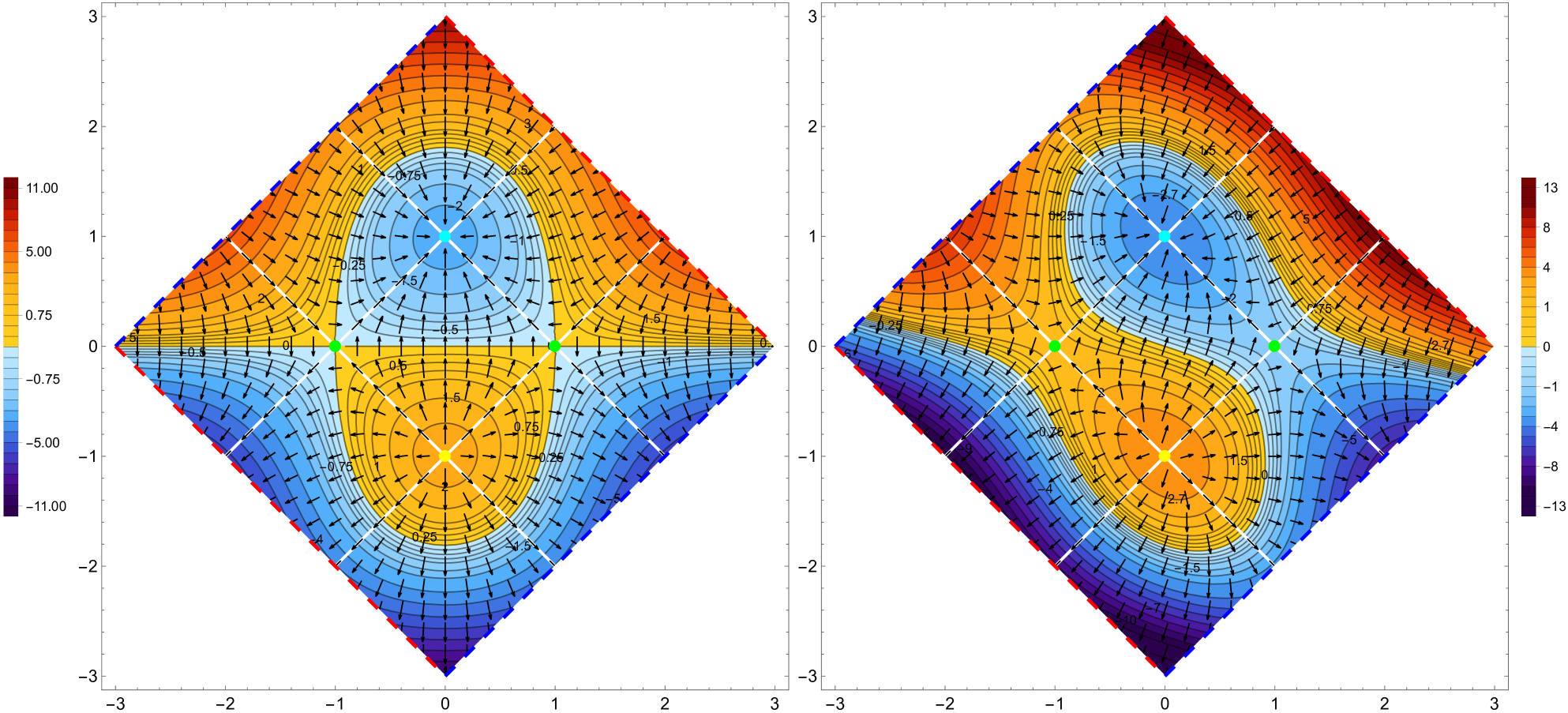
Figure 8: Vector fields for the mean values of the charge currents (7.1) in $\mathbb{M}_{\diamond}$, whose potential is the first expressions in (7.3). The CFT has $c=1$, $\kappa=3$ and either equal chemical potentials $\mu_{+}=\mu_{-}=2\pi/L$ (left panel) or different chemical potentials $\mu_{+}=4\pi/L$ and $\mu_{-}=2\pi/L$ (right panel). Here $L=6$ and $\ell=2$.

Consistency between (7.1)-(7.4) and the mean values of the currents occurs because (7.4) and (6.9) are related as follows

$$-\,\partial_{u}\,g_{{}_{\textrm{\tiny$L$}}}\!(u)=V_{L}(u)\,.$$ (7.5)

Combining (5.14), (6.11) and (7.5), it is straightforward to find that the functions (5.13) and (7.4) are related as follows

$$\partial_{u}g_{L}(u)=\frac{\partial_{u}\tilde{g}\big{(}{\rm e}^{2\pi{\rm i}u/L}\big{)}}{\big{[}\partial_{u}\big{(}{\rm e}^{2\pi{\rm i}u/L}\big{)}\big{]}^{2}}$$ (7.6)

where $\tilde{g}(u)$ is defined as (5.13) where $a$ and $b$ are replaced by ${\rm e}^{2\pi{\rm i}a/L}$ and ${\rm e}^{2\pi{\rm i}b/L}$ respectively. Moreover, the infinite volume limit $L\to+\infty$ of (7.4) gives (5.13); hence the potentials (5.12) obtained for the CFT on the line are the infinite volume limit of (7.3).

The vector fields $\boldsymbol{j}(x,t)$ and $\boldsymbol{k}(x,t)$, which are well defined in $\mathbb{M}_{\diamond}$, have vanishing fluxes through the solid white lines in Fig. 8 and Fig. 9; indeed, the absolute value of the ratio of theirs components is equal to one along these lines. These vanishing fluxes lead us to consider the total charges in the diamond $\mathcal{D}_{A}$. In the finite volume and finite density representation, from (6.1) and (5.16), for the mean values of (3.17) and (3.23) we find respectively

$$\langle Q_{A}\rangle_{{}_{\textrm{\tiny$L,\mu$}}}\!=\langle Q_{A}\rangle_{\mu}\;\;\;\qquad\;\;\;\langle\widetilde{Q}_{A}\rangle_{{}_{\textrm{\tiny$L,\mu$}}}\!=\langle\widetilde{Q}_{A}\rangle_{\mu}\,.$$ (7.7)

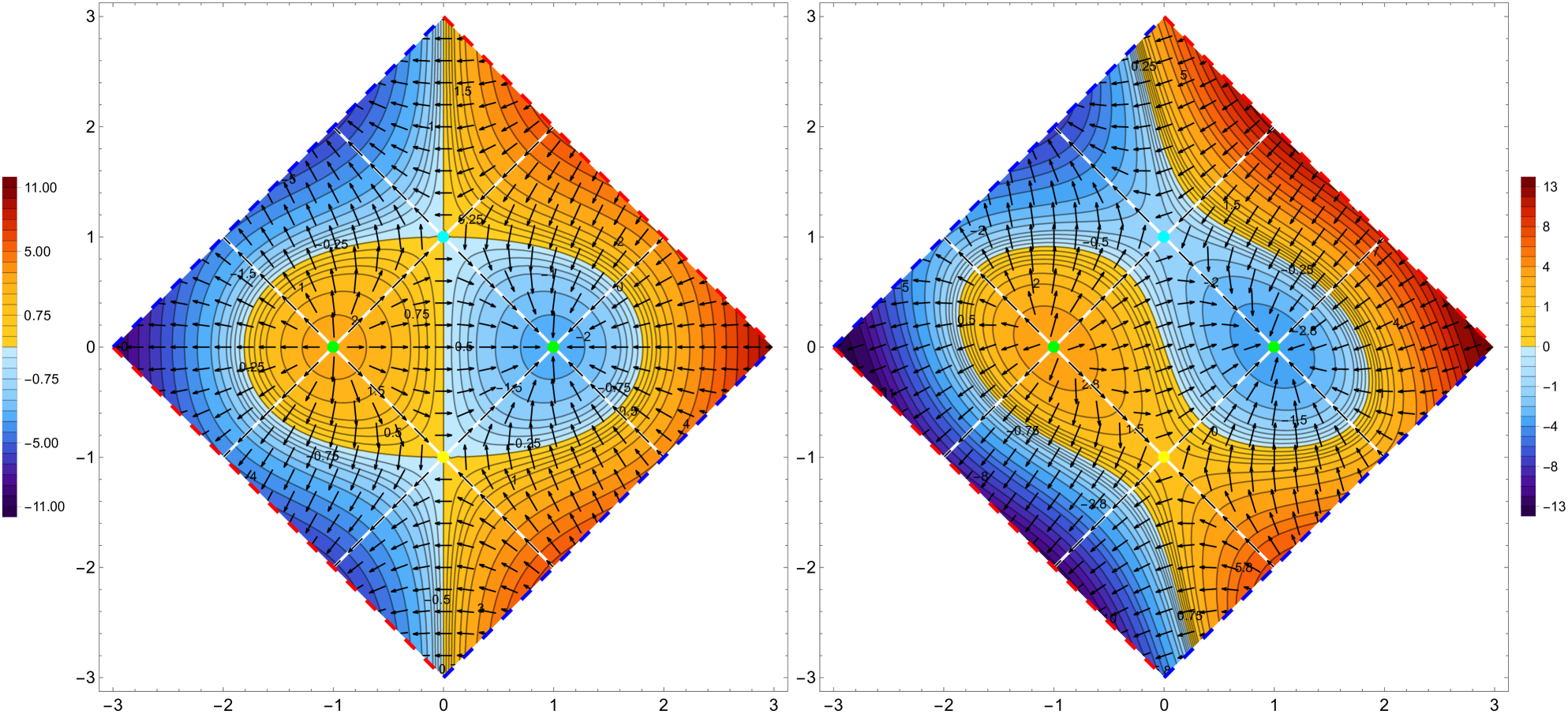
Figure 9: Vector fields for the mean values of the helicity currents (7.2) in $\mathbb{M}_{\diamond}$, whose potential is the second expressions in (7.3), for either equal (left panel) or different (right panel) chemical potentials, in the same setup of Fig. 8.

It is worth considering the line integrals of the curl free vector fields $\boldsymbol{j}(x,t)$ and $\boldsymbol{k}(x,t)$ along curves anchored to the opposite vertices of $\mathcal{D}_{A}$, as done in Sec. 5.1. The results read

$$\mathcal{L}[\boldsymbol{j}]\big{(}\gamma(P_{a}\to P_{b})\big{)} = \,\mathsf{W}_{L,j}\big{|}_{P_{a}}-\mathsf{W}_{L,j}\big{|}_{P_{b}}=-\frac{2\pi}{3}\,\langle\widetilde{Q}_{A}\rangle_{\mu}\,M(\pi\ell/L)$$ (7.8)

$$\rule{0.0pt}{22.76228pt}\mathcal{L}[\boldsymbol{j}]\big{(}\gamma(P_{-\infty}\to P_{+\infty})\big{)} = \,\mathsf{W}_{L,j}\big{|}_{P_{-\infty}}-\mathsf{W}_{L,j}\big{|}_{P_{+\infty}}=-\frac{2\pi}{3}\,\langle Q_{A}\rangle_{\mu}\,M(\pi\ell/L)$$ (7.9)

and

$$\mathcal{L}[\boldsymbol{k}]\big{(}\gamma(P_{a}\to P_{b})\big{)} = \,\mathsf{W}_{L,k}\big{|}_{P_{a}}-\mathsf{W}_{L,k}\big{|}_{P_{b}}=-\frac{2\pi}{3}\,\langle Q_{A}\rangle_{\mu}\,M(\pi\ell/L)$$ (7.10)

$$\rule{0.0pt}{22.76228pt}\mathcal{L}[\boldsymbol{k}]\big{(}\gamma(P_{-\infty}\to P_{+\infty})\big{)} = \,\mathsf{W}_{L,k}\big{|}_{P_{-\infty}}-\mathsf{W}_{L,k}\big{|}_{P_{+\infty}}=-\frac{2\pi}{3}\,\langle\widetilde{Q}_{A}\rangle_{\mu}\,M(\pi\ell/L)$$ (7.11)

where

$$M(y)\equiv\frac{3}{y^{2}}\Big{(}1-y\cot(y)\Big{)}\,.$$ (7.12)

Since $M(\pi\ell/L)\to 1$ as $L/\ell\to+\infty$, the line integrals (7.8)-(7.9) and (7.10)-(7.11) become respectively (5.17)-(5.18) and (5.19)-(5.20) in the infinite volume limit. When $\mu_{+}=\mu_{-}$, the line integrals in (7.8) and (7.11) vanish (see also the left panel of Fig. 8 and Fig. 9 respectively).

The mean values of the energy currents $\langle\mathcal{J}_{x}(\tau;x,t)\rangle_{{}_{\textrm{\tiny$L,\mu$}}}$ and $\langle\mathcal{J}_{t}(\tau;x,t)\rangle_{{}_{\textrm{\tiny$L,\mu$}}}$ for the two-dimensional CFT in $\mathbb{M}_{\diamond}$ provide the components of the vector field $\boldsymbol{\mathcal{J}}(x,t)$. From the expressions of the operators in (3.29)-(3.2) with $C_{\mathcal{J}}=-\,\pi c/6$ (see also in the text below (5.27)), the mean values (6.1) and the velocity $V_{L}(u)$ in (6.9) characterising the representation and the bipartition we are considering, for the mean values of these energy currents we find

$$\langle\mathcal{J}_{x}(\tau;x,t)\rangle_{{}_{\textrm{\tiny$L,\mu$}}} = -\left[\left(\frac{\kappa\mu^{2}_{+}}{4\pi}-\frac{\pi c}{12L^{2}}\right)V_{L}(u_{+})^{2}-\left(\frac{\kappa\mu^{2}_{-}}{4\pi}-\frac{\pi c}{12L^{2}}\right)V_{L}(u_{-})^{2}\,\right]$$ (7.13)

and

$$\rule{0.0pt}{19.91684pt}\langle\mathcal{J}_{t}(\tau;x,t)\rangle_{{}_{\textrm{\tiny$L,\mu$}}} \equiv -\frac{\kappa}{4\pi}\,\Big{\{}\mu^{2}_{+}\,V_{L}(u_{+})^{2}+\mu^{2}_{-}\,V_{L}(u_{-})^{2}\Big{\}}$$

$$-\,\frac{c}{24\pi}\,\Big{\{}V_{L}(u_{+})^{2}\,\mathcal{V}[V_{L}](u_{+})+V_{L}(u_{-})^{2}\,\mathcal{V}[V_{L}](u_{-})\Big{\}}-\frac{\pi\,c}{6}$$ (7.14)

$$= -\left[\left(\frac{\kappa\mu^{2}_{+}}{4\pi}-\frac{\pi c}{12L^{2}}\right)V_{L}(u_{+})^{2}+\left(\frac{\kappa\mu^{2}_{-}}{4\pi}-\frac{\pi c}{12L^{2}}\right)V_{L}(u_{-})^{2}\,\right]$$ (7.15)

where the non trivial function of the spacetime position occurring in the second line of (7) can be simplified by observing that

$$V_{L}(u)^{2}\,\mathcal{V}[V_{L}](u)\,=\,-\,2\pi^{2}-\frac{2\pi^{2}}{L^{2}}\,V_{L}(u)^{2}$$ (7.16)

which becomes constant in the infinite volume limit (see (5.28)).

In a similar way, the mean values $\langle\widetilde{\mathcal{J}}_{x}(\tau;x,t)\rangle_{{}_{\textrm{\tiny$L,\mu$}}}$ and $\langle\widetilde{\mathcal{J}}_{t}(\tau;x,t)\rangle_{{}_{\textrm{\tiny$L,\mu$}}}$ of the momentum currents define the components of the vector field $\boldsymbol{\widetilde{\mathcal{J}}}(x,t)$ in $\mathbb{M}_{\diamond}$. From the expressions of the operators in (3.37)-(3.2) with $\widetilde{C}_{\mathcal{J}}=0$, the mean values (6.1) and the velocity $V_{L}(u)$ in (6.9), for the mean values of the operators (3.37) and (3.2) with $\widetilde{C}_{\mathcal{J}}=0$ in the finite density representation in $\mathbb{M}_{\diamond}$ we get respectively

$$\langle\widetilde{\mathcal{J}}_{x}(\tau;x,t)\rangle_{{}_{\textrm{\tiny$L,\mu$}}}\,=\,-\left[\left(\frac{\kappa\mu^{2}_{+}}{4\pi}-\frac{\pi c}{12L^{2}}\right)V_{L}(u_{+})^{2}+\left(\frac{\kappa\mu^{2}_{-}}{4\pi}-\frac{\pi c}{12L^{2}}\right)V_{L}(u_{-})^{2}\,\right]$$ (7.17)

and

$$\rule{0.0pt}{19.91684pt}\langle\widetilde{\mathcal{J}}_{t}(\tau;x,t)\rangle_{{}_{\textrm{\tiny$L,\mu$}}} \equiv -\frac{\kappa}{4\pi}\,\Big{\{}\mu^{2}_{+}\,V_{L}(u_{+})^{2}-\mu^{2}_{-}\,V_{L}(u_{-})^{2}\Big{\}}$$

$$-\,\frac{c}{24\pi}\,\Big{\{}V_{L}(u_{+})^{2}\,\mathcal{V}[V_{L}](u_{+})-V_{L}(u_{-})^{2}\,\mathcal{V}[V_{L}](u_{-})\Big{\}}$$ (7.18)

$$= -\left[\left(\frac{\kappa\mu^{2}_{+}}{4\pi}-\frac{\pi c}{12L^{2}}\right)V_{L}(u_{+})^{2}-\left(\frac{\kappa\mu^{2}_{-}}{4\pi}-\frac{\pi c}{12L^{2}}\right)V_{L}(u_{-})^{2}\,\right].$$ (7.19)

The additive constants in (7.13)-(7) and (7.17)-(7) have been fixed by imposing that the resulting expressions vanish at the vertices of the diamond $\mathcal{D}_{A}$.

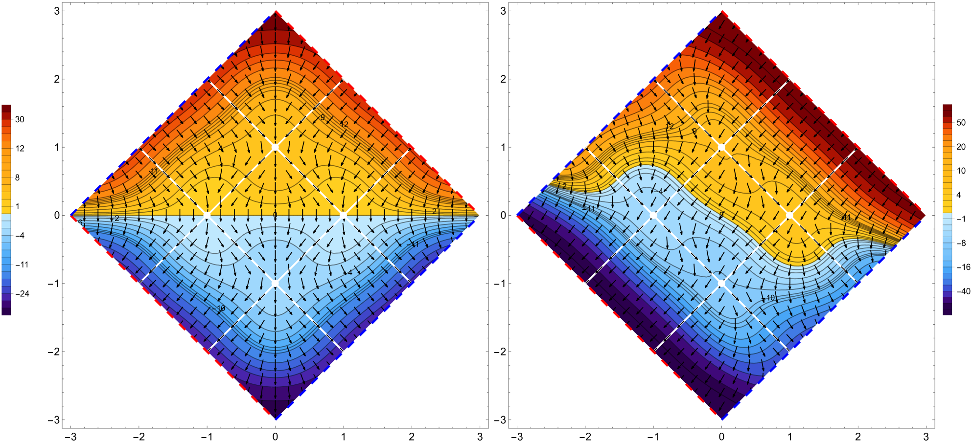
Figure 10: Vector fields for the mean values of the energy density currents (7.20) in $\mathbb{M}_{\diamond}$, whose potential is (7.22), for either equal (left panel) or different (right panel) chemical potentials, in the same setup of Fig. 8.

In Fig. 10 and Fig. 11 we show the vector fields $\boldsymbol{\mathcal{J}}(x,t)$ and $\boldsymbol{\widetilde{\mathcal{J}}}(x,t)$ in $\mathbb{M}_{\diamond}$ for the choice of the parameters described in the caption of Fig. 8. These vector fields vanish at the same critical point, which correspond to the vertices of $\mathcal{D}_{A}$. All these isolated critical points have multiplicity $2$ and Poincaré index $0$. Hence, the Poincaré-Hopf theorem can be checked also in these cases; indeed, the sum of the Poincaŕe indices in $\mathbb{M}_{\diamond}$ is zero, consistently with the fact that $\mathbb{M}_{\diamond}$ has the topology of the torus.

The vector fields $\boldsymbol{\mathcal{J}}(x,t)$ and $\boldsymbol{\widetilde{\mathcal{J}}}(x,t)$ are curl free and can be written respectively as

$$\langle\mathcal{J}_{x}(\tau;x,t)\rangle_{{}_{\textrm{\tiny$L,\mu$}}}=-\,\partial_{x}\mathsf{W}_{L,\mathcal{J}}(x,t)\;\;\;\qquad\;\;\;\langle\mathcal{J}_{t}(\tau;x,t)\rangle_{{}_{\textrm{\tiny$L,\mu$}}}=-\,\partial_{t}\mathsf{W}_{L,\mathcal{J}}(x,t)$$ (7.20)

$$\langle\widetilde{\mathcal{J}}_{x}(\tau;x,t)\rangle_{{}_{\textrm{\tiny$L,\mu$}}}=-\,\partial_{x}\mathsf{W}_{L,\widetilde{\mathcal{J}}}(x,t)\;\;\;\qquad\;\;\;\langle\widetilde{\mathcal{J}}_{t}(\tau;x,t)\rangle_{{}_{\textrm{\tiny$L,\mu$}}}=-\,\partial_{t}\mathsf{W}_{L,\widetilde{\mathcal{J}}}(x,t)$$ (7.21)

where the potentials $\mathsf{W}_{L,\mathcal{J}}$ and $\mathsf{W}_{L,\widetilde{\mathcal{J}}}$ read respectively

$$\mathsf{W}_{L,\mathcal{J}}(x,t) \equiv \left(\frac{\kappa\mu^{2}_{+}}{4\pi}-\frac{\pi c}{12L^{2}}\right)G_{L}(u_{+})-\left(\frac{\kappa\mu^{2}_{-}}{4\pi}-\frac{\pi c}{12L^{2}}\right)G_{L}(u_{-})$$ (7.22)

$$\rule{0.0pt}{19.91684pt}\mathsf{W}_{L,\widetilde{\mathcal{J}}}(x,t) \equiv \left(\frac{\kappa\mu^{2}_{+}}{4\pi}-\frac{\pi c}{12L^{2}}\right)G_{L}(u_{+})+\left(\frac{\kappa\mu^{2}_{-}}{4\pi}-\frac{\pi c}{12L^{2}}\right)G_{L}(u_{-})$$ (7.23)

in terms of the function $G_{L}(u)$ defined as follows

$$G_{L}(u) \equiv \frac{L^{3}}{2\pi\sin^{2}\!\big{[}\tfrac{\pi}{L}(b-a)\big{]}}\;\Bigg{\{}\sin\!\left(\frac{2\pi(b-u)}{L}\right)-\sin\!\left(\frac{2\pi(u-a)}{L}\right)$$ (7.24)

$$\hskip 42.67912pt+\,\frac{1}{4}\sin\!\left(\frac{4\pi}{L}\!\left(u-\frac{a+b}{2}\right)\!\right)+\frac{2\pi}{L}\left[1+\frac{1}{2}\,\cos\!\left(\frac{2\pi(b-a)}{L}\right)\right]\left(u-\frac{a+b}{2}\right)\Bigg{\}}$$

which satisfies $G_{L}\big{(}\frac{a+b}{2}\big{)}=0$; hence (7.22) and (7.23) vanish in the center of the diamond $\mathcal{D}_{A}$.

Similarly to (7.4) and (7.1)-(7.2), the function (7.24) is not periodic in $u$ and therefore the potentials (7.22) and (7.23) are not well defined in the whole spacetime $\mathbb{M}_{\diamond}$ but only in a subset of $\mathbb{M}_{\diamond}$ where a neighbourhood of boundary made by the union of the dashed straight segments in Fig. 10 and Fig. 11 has been subtracted.

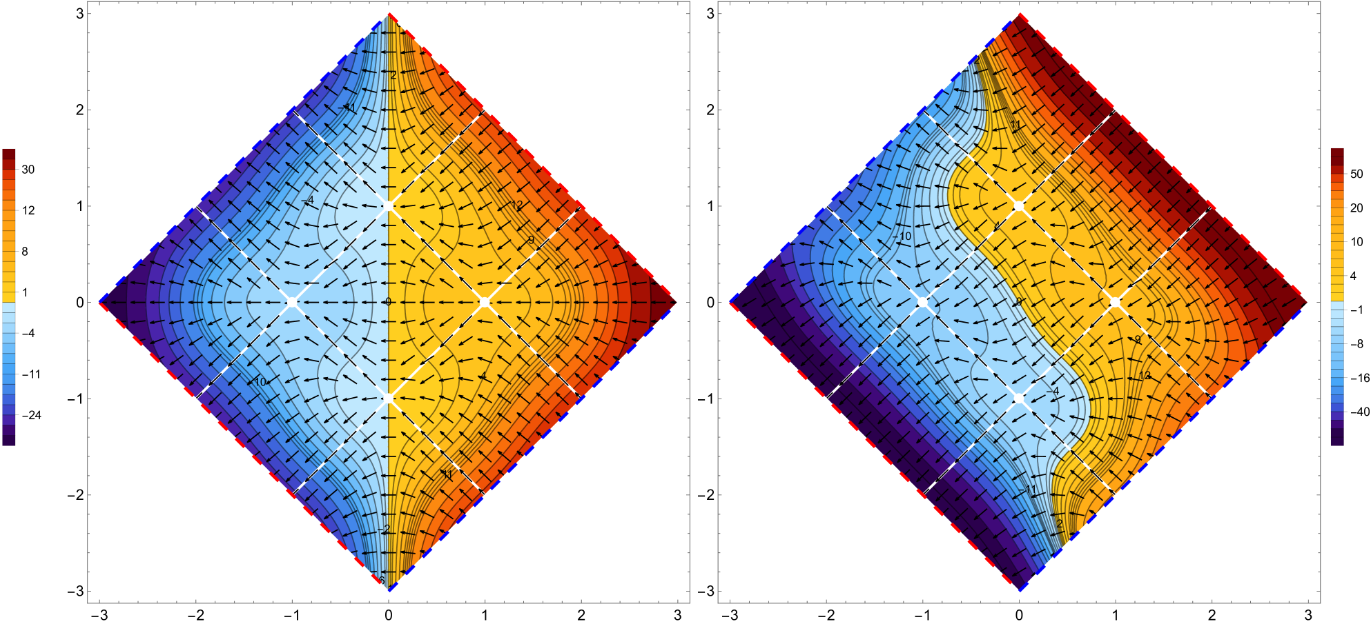
Figure 11: Vector fields for the mean values of the momentum density currents (7.21) in $\mathbb{M}_{\diamond}$, whose potential is (7.23), for either equal (left panel) or different (right panel) chemical potentials, in the same setup of Fig. 8.

Consistency among the expressions reported between (7.13) and (7.24) occurs because (7.24) and $V_{L}(u)$ in (6.9) are related as follows

$$\partial_{u}G_{L}(u)=V_{L}(u)^{2}\,.$$ (7.25)

From (5.40), (6.11) and (7.25), we observe that the functions in (5.2) and (7.24) are related as follows

$$\partial_{u}G_{L}(u)=\frac{\partial_{u}\widetilde{G}\big{(}{\rm e}^{2\pi{\rm i}u/L}\big{)}}{\big{[}\partial_{u}\big{(}{\rm e}^{2\pi{\rm i}u/L}\big{)}\big{]}^{3}}$$ (7.26)

where $\widetilde{G}(u)$ is defined as (5.2) where $a$ and $b$ are replaced by ${\rm e}^{2\pi{\rm i}a/L}$ and ${\rm e}^{2\pi{\rm i}b/L}$ respectively. In the infinite volume limit $L\to+\infty$ of (7.24) gives (5.2); hence the potentials in (7.22) and (7.23) become respectively the first and the second potential in (5.38) in this regime.

The fluxes of the vector fields $\boldsymbol{\mathcal{J}}(x,t)$ and $\boldsymbol{\widetilde{\mathcal{J}}}(x,t)$ through the straight white lines in Fig. 10 and Fig. 11 vanish, as we can show by observing that the absolute value of the ratios of their components is equal to 1 along these lines. As already highlighted in Sec. 5.2 for the corresponding vector fields on the plane, also in this case this analytic result is not properly displayed in the left panels of Fig. 10 and Fig. 11 (see around the vertices of $\mathcal{D}_{A}$) because of a failure in the graphical representation of the vector fields. A similar issue occurs in both the panels of these figures at the vertices of $\mathcal{D}_{A}$, where arrows are displayed, despite the fact that these are critical points of the vector fields. Such failures do not occur for the vector fields $\boldsymbol{j}(x,t)$ and $\boldsymbol{k}(x,t)$ in Fig. 8 and Fig. 9, whose critical points have multiplicity 1.

The line integrals of the curl free vector fields $\boldsymbol{\mathcal{J}}(x,t)$ and $\boldsymbol{\widetilde{\mathcal{J}}}(x,t)$ along curves anchored to the opposite vertices of $\mathcal{D}_{A}$ read

$$\mathcal{L}[\boldsymbol{\mathcal{J}}]\big{(}\gamma(P_{a}\to P_{b})\big{)} = \,\mathsf{W}_{L,\mathcal{J}}\big{|}_{P_{a}}-\mathsf{W}_{L,\mathcal{J}}\big{|}_{P_{b}}\,=\,-\frac{4\pi}{5}\,\widetilde{\mathsf{E}}_{A,L}\;\mathcal{M}(\pi\ell/L)$$ (7.27)

$$\rule{0.0pt}{17.07182pt}\mathcal{L}[\boldsymbol{\mathcal{J}}]\big{(}\gamma(P_{-\infty}\to P_{+\infty})\big{)} = \,\mathsf{W}_{L,\mathcal{J}}\big{|}_{P_{-\infty}}-\mathsf{W}_{L,\mathcal{J}}\big{|}_{P_{+\infty}}=\,-\frac{4\pi}{5}\,\mathsf{E}_{A,L}\;\mathcal{M}(\pi\ell/L)$$ (7.28)

and

$$\mathcal{L}[\boldsymbol{\widetilde{\mathcal{J}}}]\big{(}\gamma(P_{a}\to P_{b})\big{)} = \,\mathsf{W}_{L,\widetilde{\mathcal{J}}}\big{|}_{P_{a}}-\mathsf{W}_{L,\widetilde{\mathcal{J}}}\big{|}_{P_{b}}\,=\,-\frac{4\pi}{5}\,\mathsf{E}_{A,L}\;\mathcal{M}(\pi\ell/L)$$ (7.29)

$$\rule{0.0pt}{17.07182pt}\mathcal{L}[\boldsymbol{\widetilde{\mathcal{J}}}]\big{(}\gamma(P_{-\infty}\to P_{+\infty})\big{)} = \,\mathsf{W}_{L,\widetilde{\mathcal{J}}}\big{|}_{P_{-\infty}}-\mathsf{W}_{L,\widetilde{\mathcal{J}}}\big{|}_{P_{+\infty}}=\,-\frac{4\pi}{5}\,\widetilde{\mathsf{E}}_{A,L}\;\mathcal{M}(\pi\ell/L)$$ (7.30)

where we have introduced

$$\mathsf{E}_{A,L} \equiv \left(\frac{\kappa(\mu^{2}_{+}+\mu^{2}_{-})}{8\pi}-\frac{\pi c}{12L^{2}}\right)\frac{\pi\ell^{3}}{3}\,M(\pi\ell/L)$$ (7.31)

$$\rule{0.0pt}{19.91684pt}\widetilde{\mathsf{E}}_{A,L} \equiv \frac{\kappa(\mu^{2}_{+}-\mu^{2}_{-})}{8\pi}\;\frac{\pi\ell^{3}}{3}\,M(\pi\ell/L)$$ (7.32)

in terms of the function (7.12) (hence these expressions become the ones defined in (5.45) in the infinite volume limit, as expected) and

$$\mathcal{M}(y)\equiv\frac{5\big{[}3\cot(y)+y\big{(}2-3\csc(y)^{2}\big{)}\big{]}}{4\,y\big{[}y\cot(y)-1\big{]}}\;.$$ (7.33)

From (6.1), we notice that (7.31) and (7.32) provide the mean values of the total energy (3.32) and of the total momentum (3.39) in $\mathcal{D}_{A}$ in the finite density and finite volume representation when $f_{+}(u_{+})=f_{-}(u_{-})=0$. Instead, from (6.7), for the mean values of (3.32) and (3.39) we have $\langle E_{A}\rangle_{{}_{\textrm{\tiny$L,\mu$}}}=\langle\widetilde{E}_{A}\rangle_{{}_{\textrm{\tiny$L,\mu$}}}=0$.

Since $\mathcal{M}(\pi\ell/L)\to 1$ in the infinite volume limit, the line integrals (7.27)-(7.28) and (7.29)-(7.30) become respectively (5.41)-(5.42) and (5.43)-(5.44) in this regime. When $\mu_{+}=\mu_{-}$, the integrals in (7.28) and (7.30) vanish, as one can realise also from the left panel of Fig. 10 and Fig. 11 respectively.

By using the correlators in Sec. 6.1, also at finite volume we can introduce the modular noise power at frequency $\omega$ and in the spacetime point $(x,t)\in\mathbb{M}_{\diamond}$ generated by the various quantities as done in Sec. 5.3 for the Minkowski spacetime. In $\mathbb{M}_{\diamond}$ one introduces $P_{L,j}(\omega;x,t)$ for the charge current, $P_{L,k}(\omega;x,t)$ for the helicity current, $P_{L,\mathcal{J}}(\omega;x,t)$ for the energy current, $P_{L,\widetilde{\mathcal{J}}}(\omega;x,t)$ for the momentum current, $P_{L,\varrho}(\omega;x,t)$ for the charge density and $P_{L,\chi}(\omega;x,t)$ for the density (3.19). Since in the computation of these quantities the coincident points limit must be considered, the only difference with respect to the expressions reported in Sec. 5.3 is due to the fact that $V(u)$ must be replaced by $V_{L}(u)$ in (6.9). Thus, $P_{L,j}(\omega;x,t)=P_{j}(\omega;x,t)$, $P_{L,k}(\omega;x,t)=P_{k}(\omega;x,t)$, $P_{L,\mathcal{J}}(\omega;x,t)=P_{\mathcal{J}}(\omega;x,t)$ and $P_{L,\widetilde{\mathcal{J}}}(\omega;x,t)=P_{\widetilde{\mathcal{J}}}(\omega;x,t)$, while in $P_{L,\varrho}(\omega;x,t)$ and $P_{L,\chi}(\omega;x,t)$ do not coincide with $P_{\varrho}(\omega;x,t)$ and $P_{\chi}(\omega;x,t)$ respectively because the velocity explicitly occurs in their expressions (see (5.3)).

These observations lead to introduce $\mathcal{A}_{L}[\mathcal{O}](\omega;x,t)$ and $\mathcal{C}_{L}[\mathcal{O}](\omega;x,t)$ as the r.h.s. of (5.70) and (5.71) respectively with $\langle\dots\rangle_{\mu}^{\textrm{\tiny con}}$ replaced by $\langle\dots\rangle^{\textrm{\tiny con}}_{{}_{\textrm{\tiny$L,\mu$}}}$, finding that they satisfy the following modular fluctuation-dissipation relation

$$\mathcal{A}_{L}[\mathcal{O}](\omega;x,t)\,=\,\coth\!\left(\frac{\omega}{2}\right)\,\mathcal{C}_{L}[\mathcal{O}](\omega;x,t)$$ (7.34)

which encodes the fact that the modular evolution has a thermal nature with inverse temperature $\tilde{\beta}=1$, in agreement with the KMS condition for the modular correlators (see Sec. 6.3).

Finally, we emphasise that the heuristic picture for the transport described in the final part of Sec. 5.1 can be adapted to the finite volume case in a straightforward way.

8 Conclusions

We investigated the modular quantum transport in a two-dimensional CFT at finite density and zero temperature for the bipartition given by an interval either on the line or on the circle.

The modular flows of the operators that we have considered (primaries, currents and energy-momentum tensor) are generated by modular Hamiltonians which depend also on the chemical potentials (see (2.6), (4.10) and (6.2)) [9, 11]. Their explicit expressions can be written by specialising (2.18), (2.20), (2.23) and (2.34) to the modular evolutions corresponding to (4.11) for the interval on the infinite line and to (6.12) for the interval on the circle, as discussed in Sec. 4.2 and Sec. 6.2 respectively. From these modular flows, we have found modular continuity equations (see (3.15), (3.20), (3.28) and (3.36) specialised to $V_{+}(u)=V_{-}(u)$, which is equal to (4.7) for the interval on the line and to (6.9) for the interval on the circle) and the corresponding conserved quantities along the modular evolution (see (3.17), (3.23), (3.32), (3.39) and also (3.55) for the modular heat, in the special cases just mentioned), where the dependence on the representation occurs through the expression of the velocities.

In the finite density representations, either on the line or on the circle, the mean values of the modular currents that we have introduced naturally provide two-dimensional curl free vector fields that describe the modular quantum transport in the spacetime (see Sec. 5.1 and Sec. 5.2 for the CFT on the line and in Sec. 7 for the CFT on the circle). This modular quantum transport is different from the one discussed in [60, 61, 62], based on the Berry phase.

Finally, we have investigated the modular quantum noise power generated by various currents for a CFT either on the line or on the circle (see Sec. 5.3 and Sec. 7 respectively). A modular Johnson-Nyquist law (see (5.54), which holds also at finite volume) for the modular noise power generated by the charge current and the modular analogue of the fluctuation-dissipation relation are obtained. These results confirm the thermal nature of the modular evolution with inverse temperature $\tilde{\beta}=1$, in agreement with the KMS condition for the modular correlators (see Sec. 4.4 and Sec. 6.3). While the modular noise power generated by the charge or by the helicity current contains the coefficient occurring in the central term in (2.5), the modular noise power generated by the energy or by the momentum current contains the central charge of the CFT. Furthermore, while the modular noise power generated by these currents is independent of the spacetime position (see (5.54) and (5.61)), the modular noise power generated by the charge density depends on the position in the spacetime (see (5.69)).

The results discussed in this manuscript can be extended in various directions. In two spacetime dimensions, it is worth studying the modular transport properties for CFT at finite temperature, for either bi-local or non-local modular Hamiltonians [41, 40, 63, 64, 65, 66, 67, 68], including the ones corresponding to systems with boundaries or defects [54, 69, 70], for modular Hamiltonians in inhomogeneous systems [71] and in non-relativistic field theories [72, 11, 73]. It is relevant to explore the modular quantum transport also in higher dimensional quantum field theories [7, 8] and to investigate possible gravitational duals of these results, maybe by using [74, 75, 76]. Another direction concerns the connections between our results and the previous analyses in inhomogeneous CFT [77, 78, 79, 80, 81, 82, 26, 83, 84, 85]. Finally, it is worth exploring the modular evolution and the corresponding transport properties also in lattice models [86, 87, 88, 89, 90, 91, 92, 93, 94, 95, 96].

Acknowledgments

We are grateful to Bruno Bertini, Andrea Gambassi, Stefano Lepri, Per Moosavi, Domenico Seminara and especially Stefan Hollands, Antonio Lerario, Hong Liu and Roberto Longo for useful discussions or correspondence. ET acknowledges Center for Theoretical Physics at MIT (Boston), University of Florence and NORDITA (Stockholm) for warm hospitality and financial support during part of this work. DP has been supported by ERC under Consolidator grant number 771536 (NEMO) during his last year in SISSA.

Appendix A Basic correlators in the fundamental representation

In this appendix we summarise the one-point functions and the two-point functions of the chiral fields on the line considered in Sec. 2.1 in the fundamental representation.

A characteristic feature of this representation is the vanishing of the one-point functions

$$\langle\phi_{\pm}(u)\rangle_{{}_{0}}=\langle j_{\pm}(u)\rangle_{{}_{0}}=\langle T_{\pm}(u)\rangle_{{}_{0}}=0$$ (A.1)

hence the corresponding two-point functions coincide with their connected parts. By using the normalisation adopted in [28, 52], by conformal invariance, for the primaries we have

$$\langle\phi_{\pm}^{*}(u)\,\phi_{\pm}(v)\rangle_{{}_{0}}=\langle\phi_{\pm}(u)\,\phi_{\pm}^{*}(v)\rangle_{{}_{0}}=\frac{{\rm e}^{\mp{\rm i}\pi h_{\pm}}}{2\pi\,(u-v\mp{\rm i}\varepsilon)^{2h_{\pm}}}\,.$$ (A.2)

The normalisation of the two-point functions of $j_{\pm}(u)$ and $T_{\pm}(u)$ follow from (2.5) and (2.1) respectively. This can be shown by considering the following well known distribution

$$\frac{1}{u\pm{\rm i}\varepsilon}=\frac{1}{u}\mp{\rm i}\pi\delta(u)$$ (A.3)

and the ones obtained by taking its first, second and third derivative, that read respectively

$$\frac{1}{(u\pm{\rm i}\varepsilon)^{2}}=\frac{1}{u^{2}}\pm{\rm i}\pi\,\delta^{\prime}(u)\;\qquad\;\frac{1}{(u\pm{\rm i}\varepsilon)^{3}}=\frac{1}{u^{3}}\mp\frac{{\rm i}\pi}{2}\,\delta^{\prime\prime}(u)\;\qquad\;\frac{1}{(u\pm{\rm i}\varepsilon)^{4}}=\frac{1}{u^{4}}\pm\frac{{\rm i}\pi}{6}\,\delta^{\prime\prime\prime}(u)\,.$$ (A.4)

By conformal invariance [24], we have that

$$\langle j_{\pm}(x_{1}\pm t_{1})\,j_{\pm}(x_{2}\pm t_{2})\rangle_{{}_{0}}\,=\,\frac{C_{j_{\pm}}}{(x_{12}\pm t_{12}\mp{\rm i}\varepsilon)^{2}}$$ (A.5)

where we remind that $x_{12}\equiv x_{1}-x_{2}$ and $t_{12}\equiv t_{1}-t_{2}$. In order to fix $C_{j_{\pm}}$, from (A.5) we evaluate the expectation value of the commutator

$$\langle\big{[}\,j_{\pm}(x_{1}\pm t)\,,\,j_{\pm}(x_{2}\pm t)\,\big{]}\rangle_{{}_{0}} = C_{j_{\pm}}\!\left[\frac{1}{(x_{12}\mp{\rm i}\varepsilon)^{2}}-\frac{1}{(x_{21}\mp{\rm i}\varepsilon)^{2}}\right]$$ (A.6)

$$= C_{j_{\pm}}\!\left[\frac{1}{(x_{12}\mp{\rm i}\varepsilon)^{2}}-\frac{1}{(x_{12}\pm{\rm i}\varepsilon)^{2}}\right]\,=\,\mp\,2\pi{\rm i}\,C_{j_{\pm}}\,\delta^{\prime}(x_{12})$$

where the first distribution in (A.4) has been employed. Comparing this result with the expectation value of (2.5), one finds

$$C_{j_{\pm}}=\frac{\kappa}{4\pi^{2}}\;.$$ (A.7)

Hence, the positivity of (A.5) implies $\kappa\geqslant 0$.

A similar analysis can be performed for $T_{\pm}(u)$. In this case the two-point function is

$$\langle\,T_{\pm}(x_{1}\pm t_{1})\,T_{\pm}(x_{2}\pm t_{2})\,\rangle_{{}_{0}}=\frac{C_{T_{\pm}}}{(x_{12}\pm t_{12}\mp{\rm i}\varepsilon)^{4}}$$ (A.8)

where the constant $C_{T_{\pm}}$ has to be fixed. From (A.8), one obtains

$$\langle\big{[}\,T_{\pm}(x_{1}\pm t)\,,\,T_{\pm}(x_{2}\pm t)\,\big{]}\rangle_{{}_{0}} = C_{T_{\pm}}\!\left[\frac{1}{(x_{12}\mp{\rm i}\varepsilon)^{4}}-\frac{1}{(x_{21}\mp{\rm i}\varepsilon)^{4}}\right]$$ (A.9)

$$= C_{T_{\pm}}\!\left[\frac{1}{(x_{12}\mp{\rm i}\varepsilon)^{4}}-\frac{1}{(x_{12}\pm{\rm i}\varepsilon)^{4}}\right]=\mp\,\frac{{\rm i}\pi}{3}\,C_{T_{\pm}}\delta^{\prime\prime\prime}(x_{12})$$

which can be compared with the expectation value of (2.1), finding that consistency leads to

$$C_{T_{\pm}}=\frac{c}{8\pi^{2}}\;.$$ (A.10)

In this case, positivity of (A.8) implies the well known constraint $c\geqslant 0$ for unitary CFT.

Appendix B Currents involving the chiral primaries

In this appendix we apply to the chiral primaries the analyses discussed in Sec. 3.1 and Sec. 3.2 about the continuity equations and the conservation laws involving the electric charge, the helicity, the energy and the momentum.

Multiplying (2.11) by $V_{\pm}(u_{\pm})^{h_{\pm}-1}$ first and then taking either the sum or the difference of the resulting equations, we obtain

$$\partial_{\tau}\Phi(\tau;x,t) = \big{(}\partial_{u_{+}}+{\rm i}\,\mu_{+}\big{)}\big{[}\,V_{+}(u_{+})^{h_{+}}\,\phi_{+}(\tau,u_{+})\,\big{]}-\big{(}\partial_{u_{-}}-{\rm i}\,\mu_{-}\big{)}\big{[}\,V_{-}(u_{-})^{h_{-}}\,\phi_{-}(\tau,u_{-})\,\big{]}$$

$$\partial_{\tau}\widetilde{\Phi}(\tau;x,t) = \big{(}\partial_{u_{+}}+{\rm i}\,\mu_{+}\big{)}\big{[}\,V_{+}(u_{+})^{h_{+}}\,\phi_{+}(\tau,u_{+})\,\big{]}+\big{(}\partial_{u_{-}}-{\rm i}\,\mu_{-}\big{)}\big{[}\,V_{-}(u_{-})^{h_{-}}\,\phi_{-}(\tau,u_{-})\,\big{]}$$

where we have introduced

$$\Phi(\tau;x,t) \equiv V_{+}(u_{+})^{h_{+}-1}\,\phi_{+}(\tau,u_{+})+V_{-}(u_{-})^{h_{-}-1}\,\phi_{-}(\tau,u_{-})$$ (B.3)

$$\widetilde{\Phi}(\tau;x,t) \equiv V_{+}(u_{+})^{h_{+}-1}\,\phi_{+}(\tau,u_{+})-V_{-}(u_{-})^{h_{-}-1}\,\phi_{-}(\tau,u_{-})\,.$$ (B.4)

By using $\partial_{u_{\pm}}=\tfrac{1}{2}\big{(}\partial_{x}\pm\partial_{t}\big{)}$ and renaming (3.52) as $(\mu_{x},\mu_{t})\equiv(\mu_{e},\mu_{h})$, one finds that (B) and (B) can be written respectively as the following continuity equations

$$\partial_{\tau}\Phi(\tau;x,t)=\big{(}\partial_{\nu}+{\rm i}\,\mu_{\nu}\big{)}\Psi^{\nu}(\tau;x,t)\;\;\;\qquad\;\;\;\partial_{\tau}\widetilde{\Phi}(\tau;x,t)=\big{(}\partial_{\nu}+{\rm i}\,\mu_{\nu}\big{)}\widetilde{\Psi}^{\nu}(\tau;x,t)$$ (B.5)

where we have introduced

$$\Psi^{x}(\tau;x,t) \equiv \frac{1}{2}\big{[}\,V_{+}(u_{+})^{h_{+}}\,\phi_{+}(\tau,u_{+})-V_{-}(u_{-})^{h_{-}}\,\phi_{-}(\tau,u_{-})\,\big{]}$$ (B.6)

$$\rule{0.0pt}{18.49411pt}\Psi^{t}(\tau;x,t) \equiv \frac{1}{2}\big{[}\,V_{+}(u_{+})^{h_{+}}\,\phi_{+}(\tau,u_{+})+V_{-}(u_{-})^{h_{-}}\,\phi_{-}(\tau,u_{-})\,\big{]}$$ (B.7)

and

$$\widetilde{\Psi}^{x}(\tau;x,t)\equiv\Psi^{t}(\tau;x,t)\;\;\;\qquad\;\;\;\widetilde{\Psi}^{t}(\tau;x,t)\equiv\Psi^{x}(\tau;x,t)\,.$$ (B.8)

The differential equations in (B.5) can be expressed more conveniently in the following form

$$\partial_{\tau}\big{[}{\rm e}^{{\rm i}\mu_{\alpha}x^{\alpha}}\Phi(\tau;x,t)\big{]} = \partial_{\nu}\big{[}{\rm e}^{{\rm i}\mu_{\alpha}x^{\alpha}}\Psi^{\nu}(\tau;x,t)\big{]}$$ (B.9)

$$\partial_{\tau}\big{[}{\rm e}^{{\rm i}\mu_{\alpha}x^{\alpha}}\widetilde{\Phi}(\tau;x,t)\big{]} = \partial_{\nu}\big{[}{\rm e}^{{\rm i}\mu_{\alpha}x^{\alpha}}\widetilde{\Psi}^{\nu}(\tau;x,t)\big{]}$$ (B.10)

where $\mu_{\alpha}x^{\alpha}=\mu_{x}x+\mu_{t}t=\mu_{+}u_{+}+\mu_{-}u_{-}\,$. Considering (B.9), its r.h.s. can be written as

$$\partial_{\nu}\left[e^{i\mu_{\alpha}x^{\alpha}}\Psi^{\nu}(\tau;x,t)\right]=$$

$$\hskip-85.35826pt=\,{\rm e}^{{\rm i}\mu_{-}u_{-}}\,\partial_{u_{+}}\big{[}{\rm e}^{i\mu_{+}u_{+}}V_{+}(u_{+})^{h_{+}}\phi_{+}(\tau,u_{+})\big{]}-{\rm e}^{{\rm i}\mu_{+}u_{+}}\,\partial_{u_{-}}\big{[}{\rm e}^{{\rm i}\mu_{-}u_{-}}V_{-}(u_{-})^{h_{-}}\phi_{-}(\tau,u_{-})\big{]}$$

hence

$$\int_{\mathcal{D}_{A}}\!\!\partial_{\nu}\big{[}{\rm e}^{{\rm i}\mu_{\alpha}x^{\alpha}}\Psi^{\nu}(\tau;x,t)\big{]}{\rm d}x\,{\rm d}t = C_{a,b}(\mu_{-})\left(\,\int_{a}^{b}\partial_{u_{+}}\big{[}{\rm e}^{{\rm i}\mu_{+}u_{+}}V_{+}(u_{+})^{h_{+}}\phi_{+}(\tau,u_{+})\big{]}du_{+}\right)\hskip 39.83368pt$$

$$+\;C_{a,b}(\mu_{+})\left(\,\int_{a}^{b}\partial_{u_{-}}\big{[}{\rm e}^{{\rm i}\mu_{-}u_{-}}V_{-}(u_{-})^{h_{-}}\phi_{-}(\tau,u_{-})\big{]}du_{-}\right)=0$$

where we have introduced

$$C_{a,b}(\mu)\equiv\frac{{\rm e}^{-{\rm i}\mu a}-{\rm e}^{-{\rm i}\mu b}}{2\mu}$$ (B.13)

and (2.15) has been used. This result and the corresponding one obtained by performing a similar analysis for (B.10) imply that

$$F_{A}\equiv\int_{\mathcal{D}_{A}}\!\!{\rm e}^{{\rm i}\mu_{\alpha}x^{\alpha}}\Phi(\tau;x,t)\,{\rm d}x\,{\rm d}t = C_{a,b}(\mu_{-})\int_{a}^{b}{\rm e}^{{\rm i}\mu_{+}u_{+}}V_{+}(u_{+})^{h_{+}-1}\,\phi_{+}(\tau,u_{+})\,{\rm d}u_{+}$$

$$+\,C_{a,b}(\mu_{+})\int_{a}^{b}{\rm e}^{{\rm i}\mu_{-}u_{-}}V_{-}(u_{-})^{h_{-}-1}\,\phi_{-}(\tau,u_{-})\,{\rm d}u_{-}\hskip 28.45274pt$$

and

$$\widetilde{F}_{A}\equiv\int_{\mathcal{D}_{A}}\!\!{\rm e}^{{\rm i}\mu_{\alpha}x^{\alpha}}\,\widetilde{\Phi}(\tau;x,t)\,{\rm d}x\,{\rm d}t = C_{a,b}(\mu_{-})\int_{a}^{b}{\rm e}^{{\rm i}\mu_{+}u_{+}}V_{+}(u_{+})^{h_{+}-1}\,\phi_{+}(\tau,u_{+})\,{\rm d}u_{+}$$

$$-\,C_{a,b}(\mu_{+})\int_{a}^{b}{\rm e}^{{\rm i}\mu_{-}u_{-}}V_{-}(u_{-})^{h_{-}-1}\,\phi_{-}(\tau,u_{-})\,{\rm d}u_{-}\hskip 28.45274pt$$

are conserved, i.e. independent of $\tau$.

Appendix C Representations and automorphisms

In this appendix we describe the construction of the finite density representation of a chiral CFT on either the line $\mathbb{R}$ or on the circle $\mathbb{S}$ (see Sec. 4.1 and Sec. 6.1 respectively) using a specific automorphism $\gamma_{\mu}\equiv\gamma_{\mu_{+}}\otimes\gamma_{\mu_{-}}$ and the corresponding fundamental representation.

We begin by considering the line, where the automorphism $\gamma_{\mu}\equiv\gamma_{\mu_{+}}\otimes\gamma_{\mu_{-}}$ is defined as follows [12, 13, 97, 14, 15, 16, 26]

$$\gamma_{\mu_{\pm}}\!(\mathcal{O}_{\pm})\,\equiv\,\mathrm{e}^{\mathrm{i}D_{\mu_{\pm}}}\,\mathcal{O}_{\pm}\,\mathrm{e}^{-\mathrm{i}D_{\mu_{\pm}}}$$ (C.1)

with

$$D_{\mu_{\pm}}\,\equiv\,\pm\,\mu_{\pm}\!\int_{-\infty}^{\infty}\!u\,j_{\pm}(u)\,{\rm d}u\,.$$ (C.2)

By applying (C.1) to the fields $\phi_{\pm}$, $j_{\pm}$ and $T_{\pm}$, we find respectively

$$\gamma_{\mu_{\pm}}\!\big{(}\phi_{\pm}(u)\big{)} = {\rm e}^{\mp{\rm i}\mu_{\pm}u}\,\phi_{\pm}(u)$$ (C.3)

$$\rule{0.0pt}{19.91684pt}\gamma_{\mu_{\pm}}\!\big{(}j_{\pm}(u)\big{)} = j_{\pm}(u)-\frac{\kappa\mu_{\pm}}{2\pi}$$ (C.4)

$$\rule{0.0pt}{17.07182pt}\gamma_{\mu_{\pm}}\!\big{(}T_{\pm}(u)\big{)} = T_{\pm}(u)+\mu_{\pm}\,j_{\pm}(u)-\frac{\kappa\mu_{\pm}^{2}}{4\pi}\;.$$ (C.5)

Thus, for (2.7) we obtain

$$\gamma_{\mu_{\pm}}\!\big{(}\mathcal{T}_{\pm}(u)\big{)}\,=\,\gamma_{\mu_{\pm}}\!\big{(}T_{\pm}(u)\big{)}-\mu_{\pm}\,\gamma_{\mu_{\pm}}\!\big{(}j_{\pm}(u)\big{)}\,=\,T_{\pm}(u)+\frac{\kappa\mu_{\pm}^{2}}{4\pi}$$ (C.6)

where in the r.h.s. $T_{\pm}(u)$ occurs. The inverse of (C.3), (C.4), (C.5) and (C.6) read respectively

$$\gamma_{\mu_{\pm}}^{-1}\big{(}\phi_{\pm}(u)\big{)} = {\rm e}^{\pm{\rm i}\mu_{\pm}u}\phi_{\pm}(u)$$ (C.7)

$$\rule{0.0pt}{19.91684pt}\gamma_{\mu_{\pm}}^{-1}\big{(}j_{\pm}(u)\big{)} = j_{\pm}(u)+\frac{\kappa\mu_{\pm}}{2\pi}$$ (C.8)

$$\rule{0.0pt}{17.07182pt}\gamma_{\mu_{\pm}}^{-1}\big{(}T_{\pm}(u)\big{)} = T_{\pm}(u)-\mu_{\pm}j_{\pm}(u)-\frac{\kappa\mu_{\pm}^{2}}{4\pi}$$ (C.9)

and

$$\gamma^{-1}_{\mu_{\pm}}\big{(}\mathcal{T}_{\pm}(u)\big{)}\,=\,\mathcal{T}_{\pm}(u)-\mu_{\pm}j_{\pm}(u)-\frac{3\kappa\mu_{\pm}^{2}}{4\pi}\;.$$ (C.10)

We remark that (C.3)-(C.5) preserve the commutation relations (2.1)-(2.5).

The $n$-point function of a generic operator $\mathcal{O}$ in the finite density representation can be constructed through the automorphism (C.1) and the corresponding $n$-point function in the fundamental representation as follows

$$\langle\mathcal{O}(u_{1})\dots\mathcal{O}(u_{n})\rangle_{\textrm{\tiny$\mu_{\pm}$}}\!=\langle\gamma_{\mu_{\pm}}(\mathcal{O}(u_{1}))\dots\gamma_{\mu_{\pm}}(\mathcal{O}(u_{n}))\rangle_{{}_{0}}$$ (C.11)

The one-point functions at finite density in (4.1) are straightforwardly obtained by combining (C.11) with the fact that for a CFT in its ground state and on the line we have

$$\langle\phi_{\pm}(u)\rangle_{{}_{0}}=\,\langle j_{\pm}(u)\rangle_{{}_{0}}=\,\langle\mathcal{T}_{\pm}(u)\rangle_{{}_{0}}=\,0$$ (C.12)

The prescription (C.11) tell us that the automorphism $\gamma_{\mu_{\pm}}$ maps an operator in the finite density representation into the corresponding operator in the fundamental representation; hence $\gamma_{\mu_{\pm}}^{-1}$ can be employed to construct operators in the finite density representation from the corresponding ones in the fundamental representation. An important example is given by the modular Hamiltonians in (4.6), (4.9) and (4.10), which can be easily obtained by applying $\gamma_{\mu_{\pm}}^{-1}$ (see (C.9)) to the corresponding modular Hamiltonians in the fundamental representation.

The action of the automorphism $\gamma_{\mu_{\pm}}$ described in (C.3)-(C.6) provides also the two-point functions at finite density on the line reported in Sec. 4.1. The two-point function for the primaries in (4.2) is obtained by employing (C.3) and (4.1) as follows

$$\langle\phi_{\pm}^{*}(u)\,\phi_{\pm}(v)\rangle_{\mu_{\pm}}^{\textrm{\tiny con}}=\big{\langle}\gamma_{\mu_{\pm}}\!\big{(}\phi_{\pm}^{*}(u)\big{)}\,\gamma_{\mu_{\pm}}\!\big{(}\phi_{\pm}(v)\big{)}\big{\rangle}_{{}_{0}}^{\textrm{\tiny con}}={\rm e}^{\pm{\rm i}\mu_{\pm}(u-v)}\langle\phi_{\pm}^{*}(u)\,\phi_{\pm}(v)\rangle_{{}_{0}}^{\textrm{\tiny con}}\,.$$ (C.13)

This procedure tells us that the correlators involving primaries with different chiralities vanish also at finite density. Similarly, from (C.4) and (4.1) one finds the two-point function for the current given in (4.3) as follows

$$\langle j_{\pm}(u)\,j_{\pm}(v)\rangle_{\mu_{\pm}}^{\textrm{\tiny con}} = \langle j_{\pm}(u)\,j_{\pm}(v)\rangle_{\mu_{\pm}}-\langle j_{\pm}(u)\rangle_{\mu_{\pm}}\langle j_{\pm}(v)\rangle_{\mu_{\pm}}$$ (C.14)

$$= \langle\gamma_{\mu_{\pm}}\!\big{(}j_{\pm}(u)\big{)}\,\gamma_{\mu_{\pm}}\!\big{(}j_{\pm}(v)\big{)}\rangle_{{}_{0}}-\langle\gamma_{\mu_{\pm}}\!\big{(}j_{\pm}(u)\big{)}\rangle_{{}_{0}}\,\langle\gamma_{\mu_{\pm}}\!\big{(}j_{\pm}(v)\big{)}\rangle_{{}_{0}}$$

$$= \big{\langle}\Big{(}j_{\pm}(u)-\frac{\kappa\mu_{\pm}}{2\pi}\Big{)}\Big{(}j_{\pm}(v)-\frac{\kappa\mu_{\pm}}{2\pi}\Big{)}\big{\rangle}_{{}_{0}}-\left(\frac{\kappa\mu_{\pm}}{2\pi}\right)^{2}=\langle j_{\pm}(u)\,j_{\pm}(v)\rangle_{{}_{0}}^{\textrm{\tiny con}}\hskip 28.45274pt$$

and through similar steps also

$$\langle j_{\pm}(u)\,j_{\mp}(v)\rangle_{\mu}^{\textrm{\tiny con}}\,=\,\big{\langle}\Big{(}j_{\pm}(u)-\frac{\kappa\mu_{\pm}}{2\pi}\Big{)}\Big{(}j_{\mp}(v)-\frac{\kappa\mu_{\mp}}{2\pi}\Big{)}\big{\rangle}_{{}_{0}}-\frac{\kappa^{2}\mu_{+}\mu_{-}}{(2\pi)^{2}}=\langle j_{\pm}(u)\,j_{\mp}(v)\rangle_{{}_{0}}^{\textrm{\tiny con}}=\,0$$ (C.15)

which implies (see e.g. [26])

$$\langle j_{\pm}(u)\,j_{\mp}(v)\rangle_{\mu}=\kappa^{2}\,\frac{\mu_{+}\mu_{-}}{(2\pi)^{2}}\,.$$ (C.16)

From (C.6) and (4.1), the two-point function (4.4) is obtained as follows

$$\langle\mathcal{T}_{\pm}(u)\,\mathcal{T}_{\pm}(v)\rangle_{\mu_{\pm}}^{\textrm{\tiny con}} = \big{\langle}\bigg{(}T_{\pm}(u)+\frac{\kappa\mu^{2}_{\pm}}{4\pi}\bigg{)}\bigg{(}T_{\pm}(u)+\frac{\kappa\mu^{2}_{\pm}}{4\pi}\bigg{)}\big{\rangle}_{{}_{0}}-\left(\frac{\kappa\mu^{2}_{\pm}}{4\pi}\right)^{2}=\langle T_{\pm}(u)\,T_{\pm}(v)\rangle_{{}_{0}}^{\textrm{\tiny con}}$$

$$\langle\mathcal{T}_{\pm}(u)\,\mathcal{T}_{\mp}(v)\rangle_{\mu_{\pm}}^{\textrm{\tiny con}} = \big{\langle}\bigg{(}T_{\pm}(u)+\frac{\kappa\mu^{2}_{\pm}}{4\pi}\bigg{)}\bigg{(}T_{\mp}(u)+\frac{\kappa\mu^{2}_{\mp}}{4\pi}\bigg{)}\big{\rangle}_{{}_{0}}-\frac{\kappa^{2}\mu^{2}_{+}\mu^{2}_{-}}{(4\pi)^{2}}=\langle T_{\pm}(u)\,T_{\mp}(v)\rangle_{{}_{0}}^{\textrm{\tiny con}}=0\,.$$

The above considerations can be extended to any chiral field theory on a circle of length $L$ by fixing the periodicity of the fields. This circle is obtained by imposing the periodicity condition on the line; hence we can restrict to the the interval $[-L/2\,,\,L/2]$, imposing the following boundary conditions

$$\phi_{\pm}(L/2)=(-1)^{2h_{\pm}}\,\phi_{\pm}(-L/2)\qquad j_{\pm}(L/2)=j_{\pm}(-L/2)\qquad T_{\pm}(L/2)=T_{\pm}(-L/2)\,.$$ (C.19)

In particular, $\phi_{\pm}$ are periodic for $h_{\pm}\in\mathbb{Z}$ and anti-periodic for $h_{\pm}\in\mathbb{Z}+\frac{1}{2}$. In this case, instead of the automorphism $D_{\mu_{\pm}}$ in (C.1), one introduces

$$D_{{}_{\textrm{\tiny$L,\mu_{\pm}$}}}\,\equiv\,\pm\,\mu_{\pm}\!\int_{-L/2}^{L/2}\!u\,j_{\pm}(u)\,{\rm d}u$$ (C.20)

where $j_{\pm}(u)$ satisfies (C.19). Requiring that $\gamma_{\mu_{\pm}}$ preserves the periodicity condition (C.19) leads to the following constraint

$$\frac{L\,\mu_{\pm}}{2\pi}=n_{\pm}\;\;\;\qquad\;\;\;n_{\pm}\in\mathbb{Z}\,.$$ (C.21)

Taking into account this condition, the finite density and the zero density correlators on the circle are related as follows

$$\langle\mathcal{O}(u_{1})\dots\mathcal{O}(u_{n})\rangle_{{}_{\textrm{\tiny$L,\mu_{\pm}$}}}\!=\,\langle\gamma_{\mu_{\pm}}(\mathcal{O}(u_{1}))\dots\gamma_{\mu_{\pm}}(\mathcal{O}(u_{n}))\rangle_{{}_{\textrm{\tiny$L,0$}}}\,.$$ (C.22)

Thus, the one-point functions at finite density (6.1) can be written straightforwardly by combining (C.22) with the fact that for a CFT in its ground state and on the circle we have

$$\langle\phi_{\pm}(u)\rangle_{{}_{L,0}}=\,\langle j_{\pm}(u)\rangle_{{}_{L,0}}=\,0\;\;\;\qquad\;\;\;\langle\mathcal{T}_{\pm}(u)\rangle_{{}_{L,0}}=\langle T_{\pm}(u)\rangle_{{}_{\textrm{\tiny$L,0$}}}=\,-\frac{\pi c}{12L^{2}}\;.$$ (C.23)

Analogously, the two-point function (6.4) is obtained from (6.1) and (C.6) as follows

$$\langle{\cal T}_{\pm}(u)\,{\cal T}_{\pm}(v)\rangle_{{}_{\textrm{\tiny$L,\mu_{\pm}$}}}^{\textrm{\tiny con}} = \langle{\cal T}_{\pm}(u)\,{\cal T}_{\pm}(v)\rangle_{{}_{\textrm{\tiny$L,\mu_{\pm}$}}}-\langle{\cal T}_{\pm}(u)\rangle_{{}_{\textrm{\tiny$L,\mu_{\pm}$}}}\langle{\cal T}_{\pm}(v)\rangle_{{}_{\textrm{\tiny$L,\mu_{\pm}$}}}$$

$$= \big{\langle}\bigg{(}T_{\pm}(u)+\frac{\kappa\mu^{2}_{\pm}}{4\pi}\bigg{)}\bigg{(}T_{\pm}(u)+\frac{\kappa\mu^{2}_{\pm}}{4\pi}\bigg{)}\big{\rangle}_{{}_{\textrm{\tiny$L,0$}}}\!-\left(\frac{\kappa\mu^{2}_{\pm}}{4\pi}-\frac{\pi c}{12L^{2}}\right)^{2}$$

$$= \langle T_{\pm}(u)\,T_{\pm}(v)\rangle_{{}_{\textrm{\tiny$L,0$}}}-\left(\frac{\pi c}{12L^{2}}\right)^{2}=\,\langle T_{\pm}(u)\,T_{\pm}(v)\rangle_{{}_{\textrm{\tiny$L,0$}}}^{\textrm{\tiny con}}\,.$$ (C.24)

Summarising, the fundamental input are the correlation functions $\langle\,\cdots\rangle_{{}_{0}}$ in the ground state representation on the line. They generate, through the mapping $u\mapsto{\rm e}^{2\pi{\rm i}u/L}$, the ground state correlation functions $\langle\,\cdots\rangle_{{}_{\textrm{\tiny$L,0$}}}$ on the circle. The associated finite density correlators are obtained in turn through the automorphism $\gamma_{\mu_{\pm}}$ (see (C.11) and (C.22)). The allowed values for the chemical potential are $\mu_{\pm}\in\mathbb{R}$ on the line and $L\mu_{\pm}/(2\pi)\in\mathbb{Z}$ on the circle.

Appendix D Consistency checks for the correlators

In this appendix we describe some consistency checks for both the correlation functions (see (4.2) and (6.2)) and the modular correlators (4.4). These checks are based on the special case of free fermions (Sec. D.1), the positivity (Sec. D.2) and the properties of the entanglement spectrum (Sec. D.3). Since both chiralities can be analysed in the same way, we focus on the right movers $\phi_{+}(u)$, by setting $\phi_{+}(u)\equiv\phi(u)$, $h_{+}\equiv h$ and $\mu_{+}\equiv\mu$ throughout this appendix, to enlighten the notation.

D.1 Fermionic correlators at finite density

In order to check the first expression in (4.2) in a special case, let us consider the free chiral fermion on the line, whose two-point function at finite density can be written through the Fermi-Dirac distribution as follows

$$C(u,v)=\int_{\mathbb{R}}\frac{{\rm d}p}{2\pi}\int_{\mathbb{R}}\frac{{\rm d}k}{2\pi}\;{\rm e}^{{\rm i}(pu-kv)}\;\frac{2\pi\,\delta(u-v)}{1+{\rm e}^{\beta(p-\mu)}}\,=\,\int_{\mathbb{R}}\frac{{\rm d}p}{2\pi}\;{\rm e}^{{\rm i}p(u-v)}\;\frac{1}{1+{\rm e}^{\beta(p-\mu)}}$$ (D.1)

which can be regularised at $p\to-\infty$ by introducing the infinitesimal $\varepsilon>0$ as follows

$$C_{\varepsilon}(u,v)\equiv\int_{\mathbb{R}}\frac{{\rm d}p}{2\pi}\;{\rm e}^{{\rm i}p(u-v-{\rm i}\varepsilon)}\;\frac{1}{1+{\rm e}^{\beta(p-\mu)}}$$ (D.2)

the limit of this expression at zero temperature reads

$$\lim_{\beta\to+\infty}C_{\varepsilon}(u,v) = \int_{\mathbb{R}}\frac{{\rm d}p}{2\pi}\;{\rm e}^{{\rm i}p(u-v-{\rm i}\varepsilon)}\;\theta(\mu-p)$$ (D.3)

$$= {\rm e}^{{\rm i}\mu(u-v)}\int_{\mathbb{R}}\frac{{\rm d}q}{2\pi}\;{\rm e}^{-{\rm i}q(u-v-{\rm i}\varepsilon)}\;\theta(q)\,=\,\frac{{\rm e}^{{\rm i}\mu(u-v)}}{2\pi{\rm i}\,(u-v-{\rm i}\varepsilon)}$$

which corresponds to the first expression in (4.2) for the right moving fields when $h_{+}=1/2$.

It is worth studying the analogue computation on the circle, in order to check (6.2) in a special case. Considering the free fermion on a circle of length $L$ satisfying anti-periodic boundary conditions we can employ the complete set of orthonormal functions $\big{\{}\frac{1}{\sqrt{L}}\,{\rm e}^{{\rm i}\,2\pi n\,u/L}\,;n\in\widetilde{\mathbb{Z}}\,\big{\}}$, where $\widetilde{\mathbb{Z}}$ denotes the set made by the half-integers. The periodic boundary conditions are more subtle in the context of entanglement [98]. The two-point function of this field can be expressed through the Fermi-Dirac distribution as follows

$$C_{L}(u,v)=\frac{1}{L}\sum_{m\,\in\,\widetilde{\mathbb{Z}}}\,\sum_{n\,\in\,\widetilde{\mathbb{Z}}}\,{\rm e}^{2\pi{\rm i}(mu-nv)/L}\,\frac{\delta_{m,n}}{1+{\rm e}^{\beta(2\pi n/L-\mu)}}\,=\frac{1}{L}\sum_{n\,\in\,\widetilde{\mathbb{Z}}}{\rm e}^{2\pi{\rm i}\,n(u-v)/L}\,\frac{1}{1+{\rm e}^{\beta(2\pi n/L-\mu)}}$$ (D.4)

which can be regularised as $n\to-\infty$ through the infinitesimal $\varepsilon>0$ as above, namely

$$C_{L,\varepsilon}(u,v)\,=\frac{1}{L}\sum_{n\,\in\,\widetilde{\mathbb{Z}}}{\rm e}^{2\pi{\rm i}\,n(u-v-{\rm i}\varepsilon)/L}\,\frac{1}{1+{\rm e}^{\beta(2\pi n/L-\mu)}}$$ (D.5)

which is convergent for both $n\to-\infty$ and $n\to+\infty$, because of $\varepsilon>0$ and $\beta>0$ respectively.

The zero temperature limit of (D.5) selects the values of $n\in\widetilde{\mathbb{Z}}$ in the series such that $2\pi\,n/L-\mu\leqslant 0$, namely $n\leqslant L\mu/(2\pi)$. Since $L\mu/(2\pi)\in\mathbb{Z}$ (see Appendix C), the values of $n$ providing a non-vanishing contribution to (D.5) in the zero temperature limit are given by $n=L\mu/(2\pi)+\tilde{n}$ with $\tilde{n}\in\widetilde{\mathbb{Z}}_{-}$, being $\widetilde{\mathbb{Z}}_{-}$ made by the half-integer and negative numbers (in particular, we have that $n<L\mu/(2\pi)$). Thus, the zero temperature limit of (D.5) when $L\mu/(2\pi)\in\mathbb{Z}$ gives

$$\lim_{\beta\to+\infty}\!C_{L,\varepsilon}(u,v) = \frac{1}{L}\!\sum_{\tilde{n}\,\in\,\widetilde{\mathbb{Z}}_{-}}\!\!{\rm e}^{2\pi{\rm i}(L\mu/(2\pi)+\tilde{n})(u-v-{\rm i}\varepsilon)/L}$$

$$= \frac{{\rm e}^{{\rm i}\mu(u-v)}}{L}\!\sum_{\tilde{n}\,\in\,\widetilde{\mathbb{Z}}_{-}}\!\!{\rm e}^{2\pi{\rm i}\,\tilde{n}(u-v-{\rm i}\varepsilon)/L}\,=\,\frac{{\rm e}^{{\rm i}\mu(u-v)}}{L}\;\frac{1}{2{\rm i}\,\sin\!\big{[}\pi(u-v-{\rm i}\varepsilon)/L\big{]}}$$

which corresponds to (6.2) for the right moving fields and specialised to $h_{+}=1/2$.

D.2 Positivity

Assuming that we are dealing with a unitary CFT, the positivity of the scalar product $(\cdot\,,\cdot)$ in the state space implies that

$$\big{(}\mathcal{O}(f)\,\Omega_{\mu}\,,\,\mathcal{O}(f)\,\Omega_{\mu}\big{)}\geqslant 0$$ (D.7)

where the state $\Omega_{\mu}$ characterises the finite density representation introduced in Sec. 4.1 and

$$\mathcal{O}(f)\equiv\int_{-\infty}^{\infty}\!f(u)\,\mathcal{O}(u)\,{\rm d}u$$ (D.8)

is a chiral field smeared with a generic complex test function $f$. Choosing $\mathcal{O}(u)=\phi(u)$, the inequality (D.7) implies

$$\int_{-\infty}^{\infty}\!{\rm d}u\int_{-\infty}^{\infty}\!{\rm d}v\;\overline{f(u)}\,\langle\phi^{*}(u)\phi(v)\rangle_{\mu}\,f(v)\geqslant 0$$ (D.9)

for any test function $f$. Plugging in (D.9) the explicit form (4.2) of the correlation function one gets

$$\frac{{\rm e}^{-{\rm i}\pi h}}{2\pi}\int_{-\infty}^{\infty}\!{\rm d}u\int_{-\infty}^{\infty}\!{\rm d}v\;\frac{\overline{f_{\mu}(u)}\,f_{\mu}(v)}{(u-v-{\rm i}\varepsilon)^{2h}}\geqslant 0$$ (D.10)

where $f_{\mu}(u)\equiv{\rm e}^{-{\rm i}\mu u}f(u)$ and the overline denotes complex conjugation.

The inequality (D.10) implies a condition on the dimension $h$, which is easily obtained in momentum space. In fact, performing the Fourier transform (see for instance [99]) (D.10) takes the form

$$\frac{1}{\Gamma(2h)}\int_{-\infty}^{\infty}\frac{{\rm d}p}{2\pi}\,\big{|}\widehat{f}_{\mu}(p)\big{|}^{2}\,p_{+}^{2h-1}\,=\,\frac{1}{\Gamma(2h)}\int_{0}^{\infty}\frac{{\rm d}p}{2\pi}\,\big{|}\widehat{f}_{\mu}(p)\big{|}^{2}\,p^{2h-1}\,\geqslant\,0$$ (D.11)

where the distribution $p_{+}^{\sigma}\equiv\theta(p)\,p^{\sigma}$ has been introduced. The bound (D.11) is satisfied provided that the integral converges. This is the case for large $p$, where the integrand is dominated by the exponential decay of $|\widehat{f}_{\mu}(p)|$. The convergence at $p=0$ implies that $h>0$. Summarising, for both chiralities the dimensions of the primary fields in unitary CFT satisfy

$$h_{\pm}>0\,.$$ (D.12)

Let us discuss now the impact of positivity on the modular correlator (4.4). Given the interval $A\equiv[a,b]$, we consider the chiral field (D.8) localised in $A$ assuming for the support of the test functions ${\rm supp}(f)\subset A$. Let $S$ be the conjugate linear operator occurring in the Tomita-Takesaki theorem (see Eq. (V.2.1) of [1]) which acts as follows

$$S\,\mathcal{O}(f)\,\Omega_{\mu}=\,\mathcal{O}^{*}(f)\,\Omega_{\mu}\;\;\;\qquad\;\;\;{\rm supp}(f)\subset A\,.$$ (D.13)

The unique polar decomposition of $S$ reads

$$S=J\,\Delta^{1/2}$$ (D.14)

defining the (antiunitary) modular conjugation $J$ studied in Sec. 4.3 and the self-adjoint positive (in general unbounded) modular operator $\Delta$, which satisfy

$$J=J^{*}=J^{-1}\;\;\qquad\;\;\Delta\,\Omega_{\mu}=\Omega_{\mu}\;\;\qquad\;\;J\,\Omega_{\mu}=\Omega_{\mu}\,.$$ (D.15)

The modular operator $\Delta$ is expressed in terms of the full modular Hamiltonian $K$ in (4.10) by $\Delta\equiv{\rm e}^{-K}$.

Following [100, 38, 39] (see also (4.29)-(4.32)), we introduce the reflected operator

$$\mathcal{O}^{\textrm{\tiny ref}}(f)\equiv J\,\mathcal{O}(f)\,J^{*}$$ (D.16)

By employing (D.14) and (D.15), one finds

$$\big{(}\Omega_{\mu}\,,\,\mathcal{O}^{\textrm{\tiny ref}}(f)\,\mathcal{O}(f)\,\Omega_{\mu}\big{)} = \big{(}J^{2}\,\Omega_{\mu}\,,\,J\mathcal{O}(f)J^{*}\,\mathcal{O}(f)\,\Omega_{\mu}\big{)}$$ (D.17)

$$\hskip-42.67912pt=\,\big{(}\mathcal{O}(f)J^{*}\mathcal{O}(f)\,\Omega_{\mu}\,,\,J\,\Omega_{\mu}\big{)}=\big{(}\mathcal{O}(f)J^{*}\mathcal{O}(f)\,\Omega_{\mu}\,,\,\Omega_{\mu}\big{)}$$

$$\hskip-42.67912pt=\,\big{(}\Omega_{\mu}\,,\,\mathcal{O}^{*}(f)\,J\,\mathcal{O}^{*}(f)\,\Omega_{\mu}\big{)}=\big{(}\Omega_{\mu}\,,\,\mathcal{O}^{*}(f)\,J\,S\,\mathcal{O}(f)\,\Omega_{\mu}\big{)}$$

$$\hskip-42.67912pt=\,\big{(}\Omega_{\mu}\,,\,\mathcal{O}^{*}(f)\,J^{2}\,\Delta^{1/2}\,\mathcal{O}(f)\,\Omega_{\mu}\big{)}=\big{(}\Omega_{\mu}\,,\,\mathcal{O}^{*}(f)\,\Delta^{1/2}\,\mathcal{O}(f)\,\Omega_{\mu}\big{)}$$

$$\hskip-42.67912pt=\,\big{(}\mathcal{O}(f)\,\Omega_{\mu}\,,\,\Delta^{1/2}\,\mathcal{O}(f)\,\Omega_{\mu}\big{)}\geqslant 0$$

which has been called modular reflection positivity [38]. Thus, the modular reflection positivity can be derived from the properties of $J$, the positivity of the scalar product $(\cdot\,,\cdot)$ and the positivity of the modular operator $\Delta$.

For the field $\mathcal{O}(u)=\phi(u)$ in (D.8), the inequality (D.17) takes the form

$$\int_{-\infty}^{\infty}\!{\rm d}u\int_{-\infty}^{\infty}\!{\rm d}v\;\overline{f(u)}\,\big{(}\phi(u)\,\Omega_{\mu}\,,\,{\rm e}^{-K/2}\,\phi(v)\,\Omega_{\mu}\big{)}\,f(v)\geqslant 0\,.$$ (D.18)

On the other hand, by using ${\rm e}^{-{\rm i}\tau K}\,\Omega_{\mu}=\Omega_{\mu}$, the modular evolution (2.8) and the modular correlator (4.4) for the field $\phi(u)$, one gets

$$\frac{{\rm e}^{\pm{\rm i}\mu(u-v)}}{2\pi\,{\rm e}^{i\pi h}}\,W_{+}(\tau_{12};u,v)^{2h} = \big{(}\phi(\tau_{1},u)\,\Omega_{\mu}\,,\,\phi(\tau_{2},v)\,\Omega_{\mu}\big{)}$$ (D.19)

$$= \big{(}{\rm e}^{{\rm i}\tau_{1}K}\,\phi(u)\,{\rm e}^{-{\rm i}\tau_{1}K}\,\Omega_{\mu}\,,\,{\rm e}^{{\rm i}\tau_{2}K}\,\phi(v)\,{\rm e}^{-{\rm i}\tau_{2}K}\,\Omega_{\mu}\big{)}$$

$$= \big{(}\phi(u)\,\Omega_{\mu}\,,\,{\rm e}^{-{\rm i}\tau_{12}K}\,\phi(v)\,\Omega_{\mu}\big{)}\,.$$

Combining (D.19) specialised to $\tau_{12}=-{\rm i}/2$ with (D.18), one finds

$$\int_{-\infty}^{\infty}\!{\rm d}u\int_{-\infty}^{\infty}\!{\rm d}v\;\overline{f_{\mu}(u)}\;\frac{W_{+}(-{\rm i}/2;u,v)^{2h}}{2\pi\,{\rm e}^{i\pi h}}\;f_{\mu}(v)\,\geqslant\,0$$ (D.20)

where $f_{\mu}$ has been defined in the text below (D.10) and we have that ${\rm supp}(f_{\mu})={\rm supp}(f)\subset A$. The inequality (D.20) provides a non-trivial consistency condition for the explicit expression of $W_{+}(\tau;u,v)$ in (4.44). Indeed, when $A$ has finite length we have that (4.44) for $\varepsilon=0$ and $\tau_{12}=-{\rm i}/2$ can be written as

$$W_{+}(-{\rm i}/2;u,v)^{2h}=\Bigg{(}\frac{{\rm i}}{\tfrac{b-a}{2}\,\big{[}1-s(u)\,s(v)\big{]}}\Bigg{)}^{2h}\;\;\qquad\;\;s(u)\equiv\frac{u-\tfrac{a+b}{2}}{\tfrac{b-a}{2}}\in(-1,1)\,.$$ (D.21)

Plugging this expression into (D.20) and employing the following Taylor series

$$\frac{1}{\left(1-y\right)^{h}}=\sum_{n=0}^{\infty}\alpha_{n}(h)\,y^{n}\;\;\;\qquad\;\;\;\alpha_{n}(h)\equiv\frac{1}{n!}\prod_{k=0}^{n-1}(h+k)>0$$ (D.22)

where $h>0$ and $|y|<1$, for an interval of finite length we find that the inequality (D.20) becomes equivalent to

$$\int_{-\infty}^{\infty}\!\!{\rm d}u\int_{-\infty}^{\infty}\!\!{\rm d}v\,\overline{f_{\mu}(u)}\left[\,\sum_{n=0}^{\infty}\alpha_{n}(2h)\,s(u)^{n}s(v)^{n}\right]\!f_{\mu}(v)=\sum_{n=0}^{\infty}\alpha_{n}(2h)\left|\,\int_{-\infty}^{\infty}\!\!{\rm d}u\,f_{\mu}(u)\,s(u)^{n}\right|^{2}\geqslant 0$$ (D.23)

which is verified because $\alpha_{n}(2h)>0$.

In the special case of the Rindler wedge, i.e. in the limiting regime given by $b\to+\infty$, the inequality (D.20) becomes equivalent to

$$\int_{-\infty}^{\infty}\!\!{\rm d}u\int_{-\infty}^{\infty}\!\!{\rm d}v\,\overline{f_{\mu}(u)}\,\left(\frac{1}{u-a+v-a}\right)^{h}\!f_{\mu}(v)$$ (D.24)

$$=\frac{1}{2}\int_{-\infty}^{\infty}\!\!{\rm d}u\int_{-\infty}^{\infty}\!\!{\rm d}v\left(\frac{1}{u-a+v-a}\right)^{h}\left[\,\overline{f_{\mu}(u)}\,f_{\mu}(v)+\textrm{c.c.}\right]\,\geqslant\,\frac{1}{M_{f}^{h}}\left[\,\int_{-\infty}^{\infty}\!\!{\rm d}u\,f_{\mu}(u)\,\right]^{2}\geqslant\,0$$

where c.c. denotes the complex conjugate, $M_{f}\equiv\textrm{max}\big{\{}u-a+v-a>0\;;\,u,v\in\textrm{supp}(f)\big{\}}$ and the crucial inequality has been obtained by assuming that $f_{\mu}$ are real and positive functions with compact support properly included in $A=[a,+\infty)$.

The above analysis provides a non-trivial consistency check between the expression (4.44) of $W_{+}(\tau;u,v)$ and the modular reflection positivity condition (D.17).

D.3 Entanglement spectrum

As further consistency check of the modular correlator in (4.4)-(4.44), we show that

$$\big{(}\mathcal{O}(f)\,\Omega_{\mu}\,,\,\mathcal{O}(f)\,\Omega_{\mu}\big{)}\geqslant\big{(}\mathcal{O}(f)\,\Omega_{\mu}\,,\,\Delta^{1/2}\,\mathcal{O}(f)\,\Omega_{\mu}\big{)}\geqslant 0$$ (D.25)

where the first inequality comes from the fact that the spectrum of $\Delta$ (i.e. the entanglement spectrum) is a subset of $(0,1)$, while the last one corresponds to the positivity of the modular operator $\Delta$ (see (D.17)). For non-coincident $u,v\in[a,b]$, from (4.38) we introduce

$$r(u,v)\equiv-\,{\rm i}\,R(-{\rm i}/2;u,v)=\frac{(b-a)\,(u-v)}{2\big{[}\tfrac{a+b}{2}(u+v)-(u\,v+a\,b)\big{]}}\,\in\,[-1,1]$$ (D.26)

which satisfies (see also (4.45) and (D.21))

$$\frac{W_{+}(-{\rm i}/2;u,v)^{2h}}{{\rm e}^{i\pi h}}=\frac{r(u,v)}{u-v}\,.$$ (D.27)

From (D.19) specialised to $\tau_{12}=-{\rm i}/2$, (D.20) and (D.27), we obtain

$$\big{(}\phi(u)\,\Omega_{\mu}\,,\,\Delta^{1/2}\,\phi(v)\,\Omega_{\mu}\big{)} = \int_{-\infty}^{\infty}\!{\rm d}u\int_{-\infty}^{\infty}\!{\rm d}v\;\overline{f_{\mu}(u)}\;\frac{W_{+}(-{\rm i}/2;u,v)^{2h}}{2\pi\,{\rm e}^{i\pi h}}\;f_{\mu}(v)$$

$$= \int_{-\infty}^{\infty}\!{\rm d}u\int_{-\infty}^{\infty}\!{\rm d}v\;\overline{f_{\mu}(u)}\;\frac{r(u,v)^{2h}}{2\pi\,(u-v)^{2h}}\;f_{\mu}(v)$$

$$\leqslant \int_{-\infty}^{\infty}\!{\rm d}u\int_{-\infty}^{\infty}\!{\rm d}v\;f_{\mu}(u)\;\frac{1}{2\pi\,(u-v)^{2h}}\;f_{\mu}(v)$$ (D.28)

where the inequality originates from the fact that $r(u,v)^{2}\in[0,1]$ for $u,v\in[a,b]$ and it has been obtained by assuming that $f_{\mu}$ are real and positive functions. Finally, from (4.2), one realises that the inequality in (D.3) provides the first inequality in (D.25).

Appendix E Modular evolution in the complementary region

The modular evolution of an operator localised in the region $B$ complementary to the interval $A$ can be studied by combining its modular evolution in $A$ and the modular conjugation, as obtained in (4.36). In this appendix we derive the explicit expressions of these modular evolutions for the fields $\phi_{\pm}$, $j_{\pm}$ and $\mathcal{T}_{\pm}$.

In order to specify (4.36) to the primary fields $\phi_{\pm}$, by employing (2.18), (2.20) and (4.29), let us consider

$$\hskip-17.07182pt{\rm e}^{{\rm i}K\tau}\big{(}J\,\phi_{\pm}(u)\,J\,\big{)}\,{\rm e}^{-{\rm i}K\tau}=\;\mathrm{e}^{\mp{\rm i}\mu_{\pm}(\mathsf{j}(u)-u)}\,\mathsf{j}^{\prime}(u)^{h_{\pm}}\,{\rm e}^{{\rm i}K\tau}\phi_{\pm}^{*}(\,\mathsf{j}(u))\,{\rm e}^{-{\rm i}K\tau}$$

$$=\,\mathrm{e}^{\mp{\rm i}\mu_{\pm}(\mathsf{j}(u)-u)}\,\mathsf{j}^{\prime}(u)^{h_{\pm}}\Big{[}\,\mathrm{e}^{\mp\mathrm{i}\mu_{\pm}(\xi_{\pm}(\tau,\,\mathsf{j}(u))-\mathsf{j}(u))}\Big{(}\partial_{v}\xi_{\pm}(\tau,v)\big{|}_{v=\mathsf{j}(u)}\Big{)}^{h_{\pm}}\phi_{\pm}^{*}\big{(}\xi_{\pm}(\tau,\mathsf{j}(u))\big{)}\Big{]}$$

$$=\,\mathrm{e}^{\mp\mathrm{i}\mu_{\pm}(\xi_{\pm}(\tau,\,\mathsf{j}(u))-u)}\big{[}\partial_{u}\xi_{\pm}(\tau,\mathsf{j}(u))\big{]}^{h_{\pm}}\,\phi_{\pm}^{*}\big{(}\xi_{\pm}(\tau,\mathsf{j}(u))\big{)}\,.$$ (E.1)

Then, the r.h.s. of (4.36) is obtained by applying $J(\cdot)J$ to (E); hence, by using (4.30), for the primaries we find

$$\phi_{\pm}(\tau,u)=\mathrm{e}^{\pm\mathrm{i}\mu_{\pm}(\tilde{\xi}_{\pm}(\tau,u)-u)}\big{(}\partial_{u}\tilde{\xi}_{\pm}(\tau,u)\big{)}^{h_{\pm}}\phi_{\pm}\big{(}\tilde{\xi}_{\pm}(\mathsf{\tau,}u))\big{)}$$ (E.2)

with $\tilde{\xi}_{\pm}(\tau,u)$ being defined as follows

$$\tilde{\xi}_{\pm}(\tau,u)\equiv\,\mathsf{j}\big{(}\xi_{\pm}(\tau,\mathsf{j}(u))\big{)}=\xi_{\pm}(\tau,u)$$ (E.3)

where (4.21) has been used in the last step. This result tells us that, for the modular evolution, the expression (2.18) combined with (4.11) holds also for $u\notin A$. The above analysis can be adapted to the finite volume case by replacing $\mathsf{j}(u)$ with $\mathsf{j}_{L}(u)$ and $\xi(\tau,u)$ with $\xi_{L}(\tau,u)$ (see (6.18) and (6.12) respectively), finding the same conclusion in terms of (6.12).

As for the chiral currents $j_{\pm}$, from the r.h.s. of (4.36), (2.23) and (4.31) we have that

$${\rm e}^{{\rm i}K\tau}\big{(}J\,j_{\pm}(u)\,J\,\big{)}\,{\rm e}^{-{\rm i}K\tau}=\mathsf{j}^{\prime}(u)\;{\rm e}^{{\rm i}K\tau}j_{\pm}(\,\mathsf{j}(u))\,{\rm e}^{-{\rm i}K\tau}-\frac{\kappa\mu_{\pm}}{2\pi}\big{[}1-\mathsf{j}^{\prime}(u)\big{]}$$

$$=\,\mathsf{j}^{\prime}(u)\!\left[\,\partial_{v}\xi_{\pm}(\tau,v)\big{|}_{v=\mathsf{j}(u)}\,j_{\pm}\big{(}\xi_{\pm}(\tau,\mathsf{j}(u))\big{)}-\frac{\kappa\mu_{\pm}}{2\pi}\left(1-\left.\partial_{v}\xi_{\pm}(\tau,v)\right|_{v=\mathsf{j}(u)}\right)\right]-\frac{\kappa\mu_{\pm}}{2\pi}\big{[}1-\mathsf{j}^{\prime}(u)\big{]}$$

$$=\,\partial_{u}\xi_{\pm}(\tau,\mathsf{j}(u))\,j_{\pm}\big{(}\xi_{\pm}(\tau,\mathsf{j}(u))\big{)}-\frac{\kappa\mu_{\pm}}{2\pi}\big{[}1-\partial_{u}\xi_{\pm}(\tau,\mathsf{j}(u))\big{]}\,.$$ (E.4)

By applying $J(\cdot)J$ to (E), one gets the r.h.s. of (4.36) specified to this case. Hence, by employing again (4.31), we obtain

$$j_{\pm}(\tau,u) = \,\partial_{u}\xi_{\pm}(\tau,\mathsf{j}(u))\left[\,\mathsf{j}^{\prime}(v)\big{|}_{v=\xi_{\pm}(\tau,\,\mathsf{j}(u))}\,j_{\pm}\big{(}\,\mathsf{j}(\xi_{\pm}(\tau,\mathsf{j}(u)))\big{)}-\frac{\kappa\mu_{\pm}}{2\pi}\left(1-\left.\mathsf{j}^{\prime}(v)\right|_{v=\xi_{\pm}(\tau,\,\mathsf{j}(u))}\right)\right]$$

$$-\,\frac{\kappa\mu_{\pm}}{2\pi}\big{[}1-\partial_{u}\xi_{\pm}(\tau,\mathsf{j}(u))\big{]}$$

$$= \partial_{u}\tilde{\xi}_{\pm}(\tau,u)\,j_{\pm}\big{(}\tilde{\xi}_{\pm}(\tau,u)\big{)}-\frac{\kappa\mu_{\pm}}{2\pi}\big{[}1-\partial_{u}\tilde{\xi}_{\pm}(\tau,u)\big{]}$$ (E.5)

in terms of (E.9). Thus, as for the modular evolution of the chiral currents, the expression (2.23) combined with (4.11) holds also for $u\notin A$. This conclusion is found also in the finite volume case, once $\xi(\tau,u)$ is replaced by $\xi_{L}(\tau,u)$ given in (6.12), as one obtains by repeating the above analysis replacing also $\mathsf{j}(u)$ with $\mathsf{j}_{L}(u)$ given in (6.18).

In the finite volume case, for (2.7), from the r.h.s. of (4.36), (6.21) and (2.34) we arrive to

$$\mathrm{e}^{\mathrm{i}K\tau}\big{(}J\,\mathcal{T}_{\pm}(u)\,J\,\big{)}\,\mathrm{e}^{-\mathrm{i}K\tau}=\,\mathsf{j}_{L}^{\prime}(u)^{2}\,\mathrm{e}^{iK\tau}\,\mathcal{T}_{\pm}(\,\mathsf{j}_{L}(u))\,\mathrm{e}^{-iK\tau}+\left(\frac{\kappa\mu^{2}_{\pm}}{4\pi}-\frac{\pi c}{12L^{2}}\right)\left[\,1-\mathsf{j}^{\prime}_{L}(u)^{2}\,\right]$$

$$=\,\mathsf{j}_{L}^{\prime}(u)^{2}\;\bigg{\{}\left(\partial_{v}\xi_{L,\pm}(\tau,v)\big{|}_{v=\mathsf{j}_{L}(u)}\right)^{2}\,\mathcal{T}_{\pm}\big{(}\xi_{\pm}(\tau,\mathsf{j}_{L}(u))\big{)}+\frac{\kappa\mu_{\pm}^{2}}{4\pi}\left[\,1-\left(\left.\partial_{v}\xi_{\pm}(\tau,v)\right|_{v=\mathsf{j}_{L}(u)}\right)^{2}\,\right]$$

$$\hskip 56.9055pt-\,\frac{c}{24\pi}\,\mathcal{S}_{v}[\xi_{\pm}](\tau,v)\big{|}_{v=\mathsf{j}_{L}(u)}\,\bigg{\}}+\left(\frac{\kappa\mu^{2}_{\pm}}{4\pi}-\frac{\pi c}{12L^{2}}\right)\left[\,1-\mathsf{j}^{\prime}_{L}(u)^{2}\,\right]$$

$$=\,\big{(}\partial_{u}\xi_{\pm}(\tau,\mathsf{j}_{L}(u))\big{)}^{2}\,\mathcal{T}_{\pm}\big{(}\xi_{\pm}(\tau,\mathsf{j}_{L}(u))\big{)}+\frac{\kappa\mu_{\pm}^{2}}{4\pi}\left[\,1-\big{(}\partial_{u}\xi_{\pm}(\tau,\mathsf{j}_{L}(u))\big{)}^{2}\,\right]$$

$$\hskip 17.07182pt-\,\frac{c}{24\pi}\;\mathsf{j}_{L}^{\prime}(u)^{2}\,\mathcal{S}_{v}[\xi_{\pm}](\tau,v)\big{|}_{v=\mathsf{j}_{L}(u)}-\frac{\pi c}{12L^{2}}\left[\,1-\mathsf{j}^{\prime}_{L}(u)^{2}\,\right]$$

$$=\,\big{(}\partial_{u}\xi_{\pm}(\tau,\mathsf{j}_{L}(u))\big{)}^{2}\,\mathcal{T}_{\pm}\big{(}\xi_{\pm}(\tau,\mathsf{j}_{L}(u))\big{)}+\frac{\kappa\mu_{\pm}^{2}}{4\pi}\left[\,1-\big{(}\partial_{u}\xi_{\pm}(\tau,\mathsf{j}_{L}(u))\big{)}^{2}\,\right]-\frac{c}{24\pi}\;\mathcal{S}_{u}[\xi_{\pm}\circ\mathsf{j}_{L}](u)$$

where the following identity for the Schwarzian derivative

$$g^{\prime}(u)^{2}\,\mathcal{S}_{v}[f](v)\big{|}_{v=g(u)}=\,\mathcal{S}_{u}[f\circ g](u)-\mathcal{S}_{u}[g](u)$$ (E.7)

and (6.17) have been employed. By applying $J(\cdot)J$ to (E) and then using (6.21), we get

$$\mathcal{T}_{\pm}(\tau,u)\,=\,\big{(}\partial_{u}\tilde{\xi}_{\pm}(\tau,\mathsf{j}_{L}(u))\big{)}^{2}\,\mathcal{T}_{\pm}(\,\mathsf{j}_{L}(u))+\left(\frac{\kappa\mu^{2}_{\pm}}{4\pi}-\frac{\pi c}{12L^{2}}\right)\left[\,1-\big{(}\partial_{u}\tilde{\xi}_{\pm}(\tau,\mathsf{j}_{L}(u))\big{)}^{2}\,\right]$$ (E.8)

with $\tilde{\xi}_{\pm}(\tau,u)$ being defined in terms of (6.12) as follows

$$\tilde{\xi}_{\pm}(\tau,u)\equiv\,\mathsf{j}_{L}\big{(}\xi_{\pm}(\tau,\mathsf{j}_{L}(u))\big{)}=\xi_{\pm}(\tau,u)$$ (E.9)

where (6.20) has been employed in the last step. Thus, for the modular evolution of the chiral operators (2.7) we can use (6.16) combined with (4.11) also for $u\notin A$.

Appendix F Integrals for the quantum noise

In this appendix we discuss the explicit computation of the integrals occurring in Sec. 5.3. Let us consider first the following identity

$$\frac{1}{\sinh^{2}(\pi\tau\pm{\rm i}\epsilon)}\,=\,-\frac{1}{\pi}\,\partial_{\tau}\coth(\pi\tau\pm{\rm i}\epsilon)$$ (F.1)

where

$$\coth(\pi\tau\pm{\rm i}\epsilon)=\coth(\pi\tau)\mp{\rm i}\,\delta(\tau)$$ (F.2)

where in the r.h.s. the principal value regularization is assumed for the distribution $\coth(\pi\tau)$.

The first integral to consider is the one occurring in (5.56), namely

$$\lim_{\varepsilon\to 0}\,\int_{-\infty}^{\infty}\frac{{\rm e}^{{\rm i}\omega t}}{\sinh^{2}\!\big{[}\pi(t-{\rm i}\varepsilon)/\beta\big{]}}\,{\rm d}t\,=\,-\frac{\beta}{\pi}\,\lim_{\varepsilon\to 0}\,\int_{-\infty}^{+\infty}\!\mathrm{e}^{\mathrm{i}\beta\omega\tau}\,\partial_{\tau}\coth(\pi\tau-{\rm i}\epsilon)\,{\rm d}\tau$$ (F.3)

$$=\,{\rm i}\;\frac{\beta^{2}\omega}{\pi}\,\int_{-\infty}^{+\infty}\!\big{[}\coth(\pi\tau)+{\rm i}\,\delta(\tau)\big{]}\,\mathrm{e}^{\mathrm{i}\beta\omega\tau}\,{\rm d}\tau\,=\,-\frac{\beta^{2}}{\pi}\,\big{[}\,\omega\,\coth(\beta\omega/2)+\omega\,\big{]}$$

where we used (F.1), (F.2) and $\int_{-\infty}^{+\infty}\mathrm{e}^{\mathrm{i}\omega\tau}\coth(\pi\tau)\,{\rm d}\tau={\rm i}\coth(\omega/2)$. This computation can be adapted to investigate also the other integral we need, which occurs in (5.64). Indeed, by considering the following identity

$$\frac{1}{\sinh^{4}(\pi\tau\pm{\rm i}\epsilon)}\,=\,\frac{2}{3\pi}\,\partial_{\tau}\coth(\pi\tau\pm{\rm i}\epsilon)-\frac{1}{6\pi^{3}}\,\partial_{\tau}^{3}\coth(\pi\tau\pm{\rm i}\epsilon)$$ (F.4)

we find that

$$\lim_{\varepsilon\to 0}\,\int_{-\infty}^{\infty}\frac{{\rm e}^{{\rm i}\omega t}}{\sinh^{4}\!\big{[}\pi(t-{\rm i}\varepsilon)/\beta\big{]}}\,{\rm d}t$$ (F.5)

$$\,=\,\frac{\beta}{\pi}\,\lim_{\varepsilon\to 0}\,\int_{-\infty}^{+\infty}\!\left[\,\frac{2}{3}\,\partial_{\tau}\coth(\pi\tau-{\rm i}\epsilon)-\frac{1}{6\pi^{2}}\,\partial_{\tau}^{3}\coth(\pi\tau-{\rm i}\epsilon)\right]\mathrm{e}^{\mathrm{i}\beta\omega\tau}\,{\rm d}\tau$$

$$\,=\,-\,{\rm i}\,\frac{\beta^{2}\omega}{\pi}\left[\,\frac{2}{3}+\frac{(\beta\omega)^{2}}{6\pi^{2}}\,\right]\lim_{\varepsilon\to 0}\,\int_{-\infty}^{+\infty}\!\mathrm{e}^{\mathrm{i}\beta\omega\tau}\coth(\pi\tau-{\rm i}\epsilon)\,{\rm d}\tau$$

$$\,=\,\frac{\beta^{2}}{6\pi^{3}}\,\big{[}\,4\pi^{2}+(\beta\omega)^{2}\,\big{]}\,\big{[}\,\omega\coth(\beta\omega/2)+\omega\,\big{]}$$

where (F.4) and (F.2) have been employed.

References

- [1] R. Haag, “Local quantum physics: Fields, particles, algebras”, Springer-Verlag (1996).
- [2] S. Datta, “Electronic Transport in Mesoscopic Systems”, Cambridge University Press (1995).
- [3] Y. Blanter and M. Büttiker, “Shot noise in mesoscopic conductors”, Physics Reports 336, 1 (2000), arxiv:9910158.
- [4] Y. Nazarov and Y. Blanter, “Quantum Transport: Introduction to Nanoscience”, Cambridge University Press (2009).
- [5] J. Bisognano and E. Wichmann, “On the Duality Condition for a Hermitian Scalar Field”, J. Math. Phys. 16, 985 (1975).
- [6] J. Bisognano and E. Wichmann, “On the Duality Condition for Quantum Fields”, J. Math. Phys. 17, 303 (1976).
- [7] P. Hislop and R. Longo, “Modular Structure of the Local Algebras Associated With the Free Massless Scalar Field Theory”, Commun. Math. Phys. 84, 71 (1982).
- [8] H. Casini, M. Huerta and R. Myers, “Towards a derivation of holographic entanglement entropy”, JHEP 1105, 036 (2011).
- [9] G. Wong, I. Klich, L. Pando Zayas and D. Vaman, “Entanglement Temperature and Entanglement Entropy of Excited States”, JHEP 1312, 020 (2013), arxiv:1305.3291.
- [10] J. Cardy and E. Tonni, “Entanglement hamiltonians in two-dimensional conformal field theory”, J. Stat. Mech. 1612, 123103 (2016), arxiv:1608.01283.
- [11] M. Mintchev, D. Pontello, A. Sartori and E. Tonni, “Entanglement entropies of an interval in the free Schrödinger field theory at finite density”, JHEP 2207, 120 (2022), arxiv:2201.04522.
- [12] H. Araki, D. Kastler, M. Takesaki and R. Haag, “Extension of KMS States and Chemical Potential”, Commun. Math. Phys. 53, 97 (1977).
- [13] A. Liguori, M. Mintchev and L. Pilo, “Bosonization at finite temperature and anyon condensation”, Nucl. Phys. B 569, 577 (2000), hep-th/9906205.
- [14] D. Bernard and B. Doyon, “Non-Equilibrium Steady States in Conformal Field Theory”, Annales Henri Poincare 16, 113 (2015), arxiv:1302.3125.
- [15] S. Hollands and R. Longo, “Non-Equilibrium Thermodynamics and Conformal Field Theory”, Commun. Math. Phys. 357, 43 (2018), arxiv:1605.01581.
- [16] D. Bernard and B. Doyon, “Conformal field theory out of equilibrium: a review”, J. Stat. Mech. 1606, 064005 (2016), arxiv:1603.07765.
- [17] E. Akhmedov, H. Epstein and U. Moschella, “The massless thermal field and the thermal fermion bosonization in two dimensions”, JHEP 2209, 123 (2022), arxiv:2203.02747.
- [18] D. Ruelle, “Natural Nonequilibrium States in Quantum Statistical Mechanics”, J. Stat. Phys. 98, 57 (2000), math-ph/9906005.
- [19] S.-i. Sasa and H. Tasaki, “Steady State Thermodynamics”, J. Stat. Phys. 125, 125 (2006), cond-mat/0411052.
- [20] T. Kita, “Introduction to Nonequilibrium Statistical Mechanics with Quantum Field Theory”, Progress of Theoretical Physics 123, 581 (2010), arxiv:1005.0393.
- [21] A. Cappelli, M. Huerta and G. Zemba, “Thermal transport in chiral conformal theories and hierarchical quantum Hall states”, Nucl. Phys. B 636, 568 (2002), cond-mat/0111437.
- [22] M. Luscher and G. Mack, “The energy momentum tensor of critical quantum field theories in dimensions”, unpublished notes (1976).
- [23] A. A. Belavin, A. M. Polyakov and A. B. Zamolodchikov, “Infinite Conformal Symmetry in Two-Dimensional Quantum Field Theory”, Nucl. Phys. B 241, 333 (1984).
- [24] M. Luscher, “How to derive the Virasoro algebra from dilation invariance”, unpublished notes (1988).
- [25] P. Di Francesco, P. Mathieu and D. Sénéchal, “Conformal Field Theory”, Springer-Verlag (1996).
- [26] P. Moosavi, “Inhomogeneous Conformal Field Theory Out of Equilibrium”, Annales Henri Poincare, (2021), arxiv:1912.04821.
- [27] H. B. Callen, “Thermodynamics and an introduction to Thermostatistics”, John Wiley & Sons (1960).
- [28] K.-H. Rehren and B. Schroer, “Quasiprimary Fields: An Approach to Positivity of 2- Conformal Quantum Field Theory”, Nucl. Phys. B 295, 229 (1988).
- [29] M. Mintchev and E. Tonni, “Modular conjugations in 2D conformal field theory and holographic bit threads”, JHEP 2212, 149 (2022), arxiv:2209.03242.
- [30] D. Jovanovic, M. Mintchev and E. Tonni, “Modular evolutions and causality in two-dimensional conformal field theory”, arxiv:2501.11567.
- [31] M. Takesaki, “Tomita’s Theory of Modular Hilbert Algebras and its Applications”, Springer-Verlag (1970).
- [32] O. Bratteli and D. Robinson, “Operator algebras and quantum statistical mechanics 2: Equilibrium states. Models in quantum statistical mechanics”, Springer-Verlag (1996).
- [33] H. Borchers, “On revolutionizing quantum field theory with Tomita’s modular theory”, J. Math. Phys. 41, 3604 (2000).
- [34] M. Takesaki, “Theory of Operator Algebras II”, Springer (2003).
- [35] S. Caggioli, F. Gentile, D. Seminara and E. Tonni, “Holographic thermal entropy from geodesic bit threads”, JHEP 2407, 088 (2024), arxiv:2403.03930.
- [36] M. Freedman and M. Headrick, “Bit threads and holographic entanglement”, Commun. Math. Phys. 352, 407 (2017), arxiv:1604.00354.
- [37] C. Agón, J. De Boer and J. Pedraza, “Geometric Aspects of Holographic Bit Threads”, JHEP 1905, 075 (2019), arxiv:1811.08879.
- [38] H. Casini, “Wedge reflection positivity”, J. Phys. A 44, 435202 (2011), arxiv:1009.3832.
- [39] K. Papadodimas and S. Raju, “State-Dependent Bulk-Boundary Maps and Black Hole Complementarity”, Phys. Rev. D 89, 086010 (2014), arxiv:1310.6335.
- [40] R. Longo, P. Martinetti and K.-H. Rehren, “Geometric modular action for disjoint intervals and boundary conformal field theory”, Rev. Math. Phys. 22, 331 (2010).
- [41] H. Casini and M. Huerta, “Reduced density matrix and internal dynamics for multicomponent regions”, Class. Quant. Grav. 26, 185005 (2009), arxiv:0903.5284.
- [42] V. Arnol’d, “Ordinary Differential Equations”, Springer-Verlag (1992).
- [43] J. Milnor, “Topology from the Differentiable Viewpoint”, The University Press of Virginia (1965).
- [44] M. Ljubotina, M. Žnidarič and T. Prosen, “Spin diffusion from an inhomogeneous quench in an integrable system”, Nature Commun. 8, 16117 (2017), arxiv:1702.04210.
- [45] R. Landauer, “The noise is the signal”, Nature 392, 658 (1998).
- [46] C. L. Kane and M. P. A. Fisher, “Nonequilibrium noise and fractional charge in the quantum Hall effect”, Phys. Rev. Lett. 72, 724 (1994).
- [47] J. Johnson, “Thermal Agitation of Electricity in Conductors”, Phys. Rev. 32, 97 (1928).
- [48] H. Nyquist, “Thermal Agitation of Electric Charge in Conductors”, Phys. Rev. 32, 110 (1928).
- [49] R. Kubo, “The fluctuation-dissipation theorem”, Rep. Prog. Phys. 29, 255 (1966).
- [50] R. Kubo, M. Toda and N. Hashitsume, “Statistical Physics 2: Nonequilibrium statistical mechanics”, Springer-Verlag (1991).
- [51] U. Marini Bettolo Marconi, A. Puglisi, L. Rondoni and A. Vulpiani, “Fluctuation–dissipation: Response theory in statistical physics”, Phys. Rep. 461, 111 (2008), arxiv:0803.0719.
- [52] S. Hollands, “On the modular operator of mutli-component regions in chiral CFT”, Commun. Math. Phys. 384, 785 (2021), arxiv:1904.08201.
- [53] P. Ginsparg, “Applied Conformal Field Theory”, hep-th/9108028, in: “Les Houches Summer School in Theoretical Physics: Fields, Strings, Critical Phenomena”.
- [54] M. Mintchev and E. Tonni, “Modular Hamiltonians for the massless Dirac field in the presence of a boundary”, JHEP 2103, 204 (2021), arxiv:2012.00703.
- [55] I. Segal, “Causally oriented manifolds and groups”, Bull. Amer. Math. Soc. 77, 958 (1971).
- [56] I. Segal, “Mathematical Cosmology and Extragalactic Astronomy”, Academic Press (1976).
- [57] M. Luscher and G. Mack, “Global Conformal Invariance in Quantum Field Theory”, Commun. Math. Phys. 41, 203 (1975).
- [58] I. Todorov, M. Mintchev and V. Petkova, “Conformal Invariance in Quantum Field Theory”, Scuola Normale Superiore (1978).
- [59] R. Brunetti, D. Guido and R. Longo, “Modular structure and duality in conformal quantum field theory”, Commun. Math. Phys. 156, 201 (1993).
- [60] B. Czech, L. Lamprou, S. McCandlish and J. Sully, “Modular Berry Connection for Entangled Subregions in AdS/CFT”, Phys. Rev. Lett. 120, 091601 (2018), arxiv:1712.07123.
- [61] B. Czech, J. De Boer, D. Ge and L. Lamprou, “A modular sewing kit for entanglement wedges”, JHEP 1911, 094 (2019), arxiv:1903.04493.
- [62] S. Banerjee, M. Dorband, J. Erdmenger, R. Meyer and A.-L. Weigel, “Berry phases, wormholes and factorization in AdS/CFT”, JHEP 2208, 162 (2022), arxiv:2202.11717.
- [63] R. Arias, H. Casini, M. Huerta and D. Pontello, “Entropy and modular Hamiltonian for a free chiral scalar in two intervals”, Phys. Rev. D 98, 125008 (2018), arxiv:1809.00026.
- [64] D. Blanco and G. Pérez-Nadal, “Modular Hamiltonian of a chiral fermion on the torus”, Phys. Rev. D 100, 025003 (2019), arxiv:1905.05210.
- [65] P. Fries and I. Reyes, “Entanglement Spectrum of Chiral Fermions on the Torus”, Phys. Rev. Lett. 123, 211603 (2019), arxiv:1905.05768.
- [66] H. Bostelmann, D. Cadamuro and C. Minz, “On the Mass Dependence of the Modular Operator for a Double Cone”, Annales Henri Poincare 24, 3031 (2023), arxiv:2209.04681.
- [67] N. Abate, D. Blanco, M. Koifman and G. Pérez-Nadal, “Modular conjugation for multicomponent regions”, Phys. Rev. D 107, 045015 (2023), arxiv:2209.10711.
- [68] N. Abate and M. Koifman, “Modular conjugation for the chiral fermion in multicomponent regions on the torus”, Phys. Rev. D 108, 085003 (2023), arxiv:2307.11819.
- [69] M. Mintchev and E. Tonni, “Modular Hamiltonians for the massless Dirac field in the presence of a defect”, JHEP 2103, 205 (2021), arxiv:2012.01366.
- [70] F. Rottoli, S. Murciano, E. Tonni and P. Calabrese, “Entanglement and negativity Hamiltonians for the massless Dirac field on the half line”, J. Stat. Mech. 2301, 013103 (2023), arxiv:2210.12109.
- [71] E. Tonni, J. Rodríguez-Laguna and G. Sierra, “Entanglement hamiltonian and entanglement contour in inhomogeneous 1D critical systems”, J. Stat. Mech. 1804, 043105 (2018).
- [72] H. Leschke, A. Sobolev and W. Spitzer, “Scaling of Rényi Entanglement Entropies of the Free Fermi-Gas Ground State: A Rigorous Proof”, Phys. Rev. Lett. 112, 160403 (2014), arxiv:1312.6828.
- [73] M. Mintchev, D. Pontello and E. Tonni, “Entanglement entropies of an interval in the free Schrödinger field theory on the half line”, JHEP 2209, 090 (2022), arxiv:2206.06187.
- [74] S. Ryu and T. Takayanagi, “Holographic derivation of entanglement entropy from AdS/CFT”, Phys. Rev. Lett. 96, 181602 (2006), hep-th/0603001.
- [75] S. Ryu and T. Takayanagi, “Aspects of Holographic Entanglement Entropy”, JHEP 0608, 045 (2006), hep-th/0605073.
- [76] V. E. Hubeny, M. Rangamani and T. Takayanagi, “A Covariant holographic entanglement entropy proposal”, JHEP 0707, 062 (2007), arxiv:0705.0016.
- [77] G. Ramírez, J. Rodríguez-Laguna and G. Sierra, “Entanglement over the rainbow”, J. Stat. Mech. 1506, P06002 (2015), arxiv:1503.02695.
- [78] N. Allegra, J. Dubail, J.-M. Stéphan and J. Viti, “Inhomogeneous field theory inside the arctic circle”, J. Stat. Mech. 1605, 053108 (2016), arxiv:1512.02872.
- [79] J. Dubail, J.-M. Stéphan, J. Viti and P. Calabrese, “Conformal Field Theory for Inhomogeneous One-dimensional Quantum Systems: the Example of Non-Interacting Fermi Gases”, SciPost Phys. 2, 002 (2017), arxiv:1606.04401.
- [80] K. Gawedzki, E. Langmann and P. Moosavi, “Finite-time universality in nonequilibrium CFT”, J. Statist. Phys. 172, 353 (2018), arxiv:1712.00141.
- [81] E. Langmann, J. Lebowitz, V. Mastropietro and P. Moosavi, “Time evolution of the Luttinger model with nonuniform temperature profile”, Phys. Rev. B 95, 235142 (2017), arxiv:1701.06620.
- [82] E. Langmann and P. Moosavi, “Diffusive Heat Waves in Random Conformal Field Theory”, Phys. Rev. Lett. 122, 020201 (2019), arxiv:1807.10239.
- [83] R. Fan, Y. Gu, A. Vishwanath and X. Wen, “Emergent Spatial Structure and Entanglement Localization in Floquet Conformal Field Theory”, Phys. Rev. X 10, 031036 (2020), arxiv:1908.05289.
- [84] R. Fan, Y. Gu, A. Vishwanath and X. Wen, “Floquet conformal field theories with generally deformed Hamiltonians”, SciPost Phys. 10, 049 (2021), arxiv:2011.09491.
- [85] J. de Boer, V. Godet, J. Kastikainen and E. Keski-Vakkuri, “Quantum information geometry of driven CFTs”, JHEP 2309, 087 (2023), arxiv:2306.00099.
- [86] I. Peschel, “Calculation of reduced density matrices from correlation functions”, J. Phys. A 36, L205 (2003), cond-mat/0212631.
- [87] H. Casini and M. Huerta, “Entanglement entropy in free quantum field theory”, J. Phys. A 42, 504007 (2009), arxiv:0905.2562.
- [88] V. Eisler and I. Peschel, “Reduced density matrices and entanglement entropy in free lattice models”, J. Phys. A 42, 504003 (2009), arxiv:0906.1663.
- [89] R. Arias, D. Blanco, H. Casini and M. Huerta, “Local temperatures and local terms in modular Hamiltonians”, Phys. Rev. D 95, 065005 (2017), arxiv:1611.08517.
- [90] V. Eisler and I. Peschel, “Analytical results for the entanglement Hamiltonian of a free-fermion chain”, J. Phys. A 50, 284003 (2017), arxiv:1703.08126.
- [91] V. Eisler and I. Peschel, “Properties of the entanglement Hamiltonian for finite free-fermion chains”, J. Stat. Mech. 1810, 104001 (2018), arxiv:1805.00078.
- [92] V. Eisler, E. Tonni and I. Peschel, “On the continuum limit of the entanglement Hamiltonian”, J. Stat. Mech. 1907, 073101 (2019), arxiv:1902.04474.
- [93] G. Di Giulio and E. Tonni, “On entanglement hamiltonians of an interval in massless harmonic chains”, J. Stat. Mech. 2003, 033102 (2020), arxiv:1911.07188.
- [94] V. Eisler, G. Di Giulio, E. Tonni and I. Peschel, “Entanglement Hamiltonians for non-critical quantum chains”, J. Stat. Mech. 2010, 103102 (2020), arxiv:2007.01804.
- [95] V. Eisler, E. Tonni and I. Peschel, “Local and non-local properties of the entanglement Hamiltonian for two disjoint intervals”, J. Stat. Mech. 2208, 083101 (2022), arxiv:2204.03966.
- [96] N. Javerzat and E. Tonni, “On the continuum limit of the entanglement Hamiltonian of a sphere for the free massless scalar field”, JHEP 2202, 086 (2022), arxiv:2111.05154.
- [97] P. Camassa, R. Longo, Y. Tanimoto and M. Weiner, “Thermal States in Conformal QFT. II”, Commun. Math. Phys. 315, 771 (2012), arxiv:1109.2064.
- [98] I. Klich, D. Vaman and G. Wong, “Entanglement Hamiltonians for chiral fermions with zero modes”, Phys. Rev. Lett. 119, 120401 (2017), arxiv:1501.00482.
- [99] I. Gel’fand and G. Shilov, “Generalised Functions vol. I”, Academic Press (1964).
- [100] N. Landsman and C. van Weert, “Real and Imaginary Time Field Theory at Finite Temperature and Density”, Phys. Rept. 145, 141 (1987).