Finite Sample Analysis of System Poles for Ho-Kalman Algorithm

Abstract

This paper investigates the error analysis of system pole estimation in $n$-dimensional discrete-time Linear Time-Invariant systems with $m$ outputs and $p$ inputs, using the classical Ho-Kalman algorithm based on finite input-output sample data. Building upon prior work, we establish end-to-end estimation guarantees for system poles under both single-trajectory and multiple-trajectory settings. Specifically, we prove that, with high probability, the estimation error of system poles decreases at a rate of at least $\mathcal{O}\{T^{-\frac{1}{2n}}\}$ in the single-trajectory case and $\mathcal{O}\{N^{-\frac{1}{2n}}\}$ in the multiple-trajectory case, where $T$ is the length of a single trajectory, and $N$ is the number of trajectories. Furthermore, we reveal that in both settings, achieving a constant estimation accuracy for system poles requires the sample size to grow super-polynomially with respect to the larger of the two ratios, $\max\{n/m,n/p\}$. Numerical experiments are conducted to validate the non-asymptotic results of system pole estimation.

1 Introduction

Linear Time-Invariant (LTI) systems are a crucial class of models with widespread applications in finance, biology, robotics, and other engineering fields and control applications [1]. Many modern control design techniques depend on the availability of a reasonably accurate LTI state-space model of the plant to be controlled [2]. To this end, identifying the state-space model of the following Multiple-Input Multiple-Output (MIMO) LTI systems

$$x_{k+1} =Ax_{k}+Bu_{k}+w_{k},$$ (1)

$$y_{k} =Cx_{k}+Du_{k}+v_{k},$$

from input/output sample data has become one of the core problems in system analysis, design and control [3]. In the past, classical results [4, 5, 6, 7] in the identification of LTI systems have primarily focused on ensuring the asymptotic convergence properties of specific estimation schemes [8, 9], including consistency [10], asymptotic normality [11], and variance analysis [12]. In recent years, academia and industry have paid more and more attention to finite sample complexity and non-asymptotic analysis, because good error bounds are crucial for designing high-performance robust control systems and establishing end-to-end performance guarantees under finite sample conditions [13]. The research focus has shifted from asymptotic analysis based on infinite data to statistical analysis in the finite-data regime [14, 15]. In particular, with advancements in statistical learning and high-dimensional statistics [16, 17], a large number of research works [18, 19, 20, 14, 15, 21, 22, 23, 24, 25, 26, 27, 28, 13, 29, 30, 2, 31, 32, 33, 34, 35] based on finite samples have emerged in recent years, dedicated to addressing the parameter identification problem of LTI systems. A more comprehensive overview of non-asymptotic system identification can be found in [36].

When the system state can be measured accurately, i.e., when $C=I,D=\mathbf{0}$ and $v_{k}\equiv\mathbf{0}$, the system (1) is known as a fully observed LTI system. A series of recent studies [18, 19, 21, 14, 34, 13, 27] has established upper bounds on the identification error of system matrices $(A,B)$ when estimated using ordinary least-squares method (OLS), from a finite sample perspective. Beyond OLS, Jedra and Proutiere [26, 28] derives lower bounds on the sample complexity within the Probably Approximately Correct (PAC) framework for a class of locally stable algorithms. Furthermore, Tsiamis and Pappas [23] reveals that in under-actuated and under-excited LTI systems with specific structures, the worst-case sample complexity exhibits exponential growth with respect to the system dimension within the PAC framework. Recently, Chatzikiriakos and Iannelli [33] establish both upper and lower bounds on the sample complexity for identifying the system matrices $(A,B)$ from a finite set of candidates, even in absence of stability assumptions.

When $C\neq I$, the system (1) is a partially observed LTI system, wherein the identification problem becomes more challenging due to the inability to accurately measure the system state [37]. Recent works [2, 20, 30, 31, 32, 22, 35] have established high-probability upper bounds and convergence rates for the identification of the state-space realization $(A,B,C,D)$ under finite sample conditions, up to similarity transformations, achieving rates of $\mathcal{O}\{1/\sqrt{T}\}$ or $\mathcal{O}\{1/\sqrt{N}\}$ (up to logarithmic factors), where $T$ denotes the length of a single sample trajectory and $N$ denotes the number of independent sample trajectories. Among them, works [22, 35] estimate state-space models using subspace identification methods (SIM), which involve first extracting the relevant subspaces of the system from the input/output sample data matrix via a sequence of projections and regressions, and then utilizing the identified subspaces to reconstruct a realization of the corresponding state-space model. Another line of researches [2, 20, 30, 31, 32] focus on a two-step approach for estimating state-space models: First, the Markov parameters are estimated from finite sample data using the least-squares method (OLS). Subsequently, a balanced state-space realization is recovered via the Ho-Kalman algorithm based on the estimated Markov parameters. In addition, several other methods have been proposed for identifying state-space models based on finite sample data, including reinforcement learning techniques[38] and gradient descent algorithm [39].

Although finite-sample identification error analysis of the state-space realization $(A,B,C,D)$ under finite sample conditions have been established in works [2, 20, 30, 31, 32, 22, 35], there remains a lack of finite-sample identification error analysis concerning the system poles, i.e., the eigenvalues of matrix $A$. Therefore, in this paper, we focus on analyzing the finite-sample identification error associated with the system poles under the Ho-Kalman algorithm. [2] and [30] has provided high-probability upper bounds and convergence rate analyses for the identification error of the state-space realization under a single sample trajectory and multiple sample trajectories settings, respectively. Building upon the results of [2] and [30], we will establish high-probability upper bounds and convergence rates for the identification error of the system poles under both single-sample and multiple-sample trajectory settings, leveraging matrix eigenvalue perturbation theory. To the best of our knowledge, we provide the first finite sample identification analysis of the system poles for Ho-Kalman algorithm. The main contribution of this paper is as follows:

1. Based on the results of [2], we provides end-to-end estimation guarantees for the system poles using a single sample trajectory, and demonstrates that, with high probability, the estimation error of the system poles decreases at a rate of at least $\mathcal{O}\{T^{-\frac{1}{2n}}\}$, where $n$ denotes the system order, and $T$ denotes the length of a single sample trajectory.

2. Based on the results of [30], we provides end-to-end estimation guarantees for the system poles using a single sample trajectory, and demonstrates that, with high probability, the estimation error of the system poles decreases at a rate of at least $\mathcal{O}\{N^{-\frac{1}{2n}}\}$, where $N$ denotes the number of independent sample trajectories.

3. We further reveal that, under both single-sample and multiple-sample trajectory settings, achieving a constant estimation accuracy of the system poles requires the sample size to grow super-polynomially with respect to the larger of the two ratios, $\max\{n/m,n/p\}$, where $m$ and $p$ denote the input and output dimensions, respectively.

This paper is organized as follows: Section 2 formulates the identification problem and reviews OLS and Ho-Kalman algorithm. Section 3 analyzes the finite sample identification error of the system poles for Ho-Kalman algorithm. Section 4 provides numerical simulations, and finally, Section 5 concludes this paper.

Notations: $\mathbf{0}$ is an all-zero matrix of proper dimensions. For any $x\in\mathbb{R}$, $\lfloor x\rfloor$ denotes the largest integer not exceeding $x$, and $\lceil x\rceil$ denotes the smallest integer not less than $x$. The Frobenius norm is denoted by $\|A\|_{\rm F}=\sqrt{{\rm tr}\left(A^{\rm H}A\right)}$, and $\|A\|$ is the spectral norm of $A$, i.e., its largest singular value $\sigma_{\max}(A)$. $\sigma_{j}(A)$ denotes the $j$-th largest singular value of $A$, and $\sigma_{\min}(A)$ denotes the smallest non-zero singular value of $A$. $\lambda(A)$ denotes the spectrum of a square matrix $A$. The Moore-Penrose inverse of matrix $A$ is denoted by $A^{\dagger}$. $I_{n}$ denotes the $n\times n$ identity matrix. The matrix inequality $A>B$ implies that matrix $A-B$ is strictly positive semi-definite. Multivariate Gaussian distribution with mean $\mu$ and covariance $\Sigma$ is denoted by $\mathcal{N}(\mu,\Sigma)$. The big-$\mathcal{O}$ notation $\mathcal{O}\{f(n)\}$ represents a function that grows at most as fast as $f(n)$. The big-$\Omega$ notation $\Omega\{f(n)\}$ represents a function that grows at least as fast as $f(n)$. The big-$\Theta$ notation $\Theta\{f(n)\}$ represents a function that grows as fast as $f(n)$.

2 Problem Setup

We consider the identification problem on the MIMO LTI system of order $n$ evolving according to

$$x_{k+1} =Ax_{k}+Bu_{k}+w_{k},$$ (2)

$$y_{k} =Cx_{k}+Du_{k}+v_{k},$$

based on finite input/output sample data, where $x_{k}\in\mathbb{R}^{n}$, $u_{k}\in\mathbb{R}^{p}$, $y_{k}\in\mathbb{R}^{m}$ are the system state, the input and the output, respectively, and $w_{k}\sim\mathcal{N}(\mathbf{0},\mathcal{Q})$, $v_{k}\sim\mathcal{N}(\mathbf{0},\mathcal{R})$ with $\mathcal{Q},\,\mathcal{R}>\mathbf{0}$ are the i.i.d. process and measurement noise respectively and are independent from each other. $A,B,C,D$ are unknown matrices with appropriate dimensions.

Assumption 1.

For the system (2), the pair $(A,C)$ is observable, and the pair $(A,B)$ is controllable.

Remark 1.

Indeed, the system (2) is minimal in the sense of Assumption 1, i.e, the state-space realization $(A,B,C,D)$ of the system (2) has the smallest dimension among all state-space realizations with the same input-output relationship. On the other hand, it is worth noting that only the observable part of the system can be identified, and the controllability assumption of the system can ensure that all modes can be excited by the external input $u_{k}$. Therefore, Assumption 1 is necessary and well-defined.

Assumption 2.

The system order $n$ is known.

The goal of this paper is to provide a finite sample bound on the unknown system poles, i.e., the eigenvalues of matrix $A$, for Ho-Kalman algorithm.

Remark 2.

It is noteworthy that the input/output sample data correspond to an infinite number of equivalent state-space realizations, which are related through similarity transformations. Consequently, in this paper, we focus on the estimation of poles, which are uniquely determined by the spectrum $\lambda(A)$ of the matrix $A$ and remain invariant under similarity transformations. On the other hand, system poles serve as fundamental design parameters in various control strategies, including pole placement [40], $H_{\infty}$ loop shaping [41], and the root locus method [42], as they critically influence the stability and dynamic performance of the closed-loop system.

2.1 Least-Squares Procedure

Least-Squares procedure is used to recover Markov parameters from finite input/output sample data, which subsequently enables the recovery of a balanced state-space realization via Ho-Kalman algorithm. However, there are two distinct approaches for recovering Markov parameters using Least-Squares procedure:

1. Utilizing a single sample trajectory $\{(u_{k},y_{k}):0\leq k\leq T-1\}$, where $T$ represents the length of sample trajectory;

2. Utilizing multiple sample trajectories $\{(u_{k}^{(i)},y_{k}^{(i)}):0\leq k\leq K-1,1\leq i\leq N\}$, where $K$ and $N$ represent the length and number of sample trajectories, respectively.

Therefore, in this subsection, we will review these two approaches for recovering Markov parameters using least-squares procedure.

First define $G$ as as the matrix composed of the first $K$ Markov parameters as follows

$$G\triangleq\begin{bmatrix}D&CB&CAB&\cdots&CA^{K-2}B\end{bmatrix}\in\mathbb{R}^{m\times Kp},$$ (3)

where $G$ is recovered using Least-Squares procedure based on finite sample data, and then a balanced state-space realization is obtained by incorporating the Ho-Kalman algorithm.

2.1.1 Utilizing A Single Sample Trajectory

The least-squares procedure introduced next is from [2]. Given a single sample trajectory $\{(u_{k},y_{k}):0\leq k\leq T-1\}$, we generate $\overline{T}$ sub-sequences of length $K$, where $T=K+\overline{T}-1$ and $\overline{T}\geq 1$.

Define $\overline{u}_{k}$ and $\overline{w}_{k}$ as the vectors obtained by organizing the input $u_{k}$ and process noise $w_{k}$ into blocks of length $K$ as follows:

$$\overline{u}_{k}\triangleq\begin{bmatrix}u_{k}\\ u_{k-1}\\ \vdots\\ u_{k-K+1}\end{bmatrix}\in\mathbb{R}^{Kp},\quad\overline{w}_{k}\triangleq\begin{bmatrix}w_{k}\\ w_{k-1}\\ \vdots\\ w_{k-K+1}\end{bmatrix}\in\mathbb{R}^{Kn}.$$ (4)

Define the matrix $F$ as:

$$F\triangleq\begin{bmatrix}\mathbf{0}_{m\times n}&C&CA&\cdots&CA^{K-2}\end{bmatrix}\in\mathbb{R}^{m\times Kn}.$$ (5)

$$Y\triangleq\begin{bmatrix}y_{K-1}&y_{K}&\cdots&y_{T-1}\end{bmatrix}^{\top}\in\mathbb{R}^{\overline{T}\times m},\quad U\triangleq\begin{bmatrix}\overline{u}_{K-1}&\overline{u}_{K}&\cdots&\overline{u}_{T-1}\end{bmatrix}^{\top}\in\mathbb{R}^{\overline{T}\times Kp}.$$ (6)

The estimation of $G$ can be derived from solving the following least-squares problem:

$$\widehat{G}=\arg\min_{X\in\mathbb{R}^{m\times Kp}}\|Y-UX^{\top}\|_{\rm F}^{2}.$$ (7)

Thus, the least squares solution $\widehat{G}$ can be expressed as $\widehat{G}=(U^{\dagger}Y)^{\top}$, where $U^{\dagger}=(U^{\top}U)^{-1}U^{\top}$ is the left Moore-Penrose inverse of the matrix $U$.

2.1.2 Utilizing Multiple Sample Trajectories

The least-squares procedure introduced next is from [30]. We first define some notations. For each sample trajectory $i$, $i=1,2,\cdots,N$, define the input/output data as

$$y^{(i)}\triangleq\begin{bmatrix}y_{0}^{(i)}&\cdots&y_{K-1}^{(i)}\end{bmatrix}\in\mathbb{R}^{m\times K},\qquad U^{(i)}\triangleq\begin{bmatrix}u_{0}^{(i)}&u_{1}^{(i)}&\cdots&u_{K-1}^{(i)}\\ &u_{0}^{(i)}&\cdots&u_{K-2}^{(i)}\\ &&\ddots&\vdots\\ &&&u_{0}^{(i)}\end{bmatrix}\in\mathbb{R}^{pK\times K}.$$ (8)

Define the output matrix $Y$ and input matrix $U$ as

$$Y\triangleq\begin{bmatrix}y^{(1)}&\cdots&y^{(N)}\end{bmatrix}\in\mathbb{R}^{m\times NK},\quad U\triangleq\begin{bmatrix}U^{(1)}&\cdots&U^{(N)}\end{bmatrix}\in\mathbb{R}^{pK\times NK}.$$ (9)

The estimation of $G$ can be derived from solving the following least-squares problem:

$$\widehat{G}=\arg\min_{X\in\mathbb{R}^{m\times Kp}}\|Y-XU\|_{\rm F}^{2}.$$ (10)

Hence, the least squares solution $\widehat{G}$ can be expressed as $\widehat{G}=YU^{\dagger}$, where $U^{\dagger}=U^{\top}(UU^{\top})^{-1}$ is the right Moore-Penrose inverse of the matrix $U$.

2.2 Ho-Kalman Algorithm

In this subsection, we introduce the Ho-Kalman algorithm [43, 2] that generates a state-space realization $(A,B,C,D)$ from the Markov parameter matrix $G$ or its corresponding estimation $\widehat{G}$. Before continuing on, we first define the (extended) observability, controllability and the Hankel matrices $O\in\mathbb{R}^{K_{1}m\times n}$, $Q\in\mathbb{R}^{n\times(K_{2}+1)p}$ and $H\in\mathbb{R}^{K_{1}m\times(K_{2}+1)p}$ of the system (2) as

$$O \triangleq\begin{bmatrix}C^{\top}&(CA)^{\top}&\cdots&(CA^{K_{1}-1})^{\top}\end{bmatrix}^{\top},$$ (11)

$$Q \triangleq\begin{bmatrix}B&AB&\cdots&A^{K_{2}}B\end{bmatrix},$$ (12)

$$H \triangleq\begin{bmatrix}CB&CAB&\cdots&CA^{K_{2}}B\\ CAB&CA^{2}B&\cdots&CA^{K_{2}+1}B\\ \vdots&\vdots&\ddots&\vdots\\ CA^{K_{1}-1}B&CA^{K_{1}}B&\cdots&CA^{K_{1}+K_{2}-1}B\end{bmatrix}=OQ,$$ (13)

where $K=K_{1}+K_{2}+1$, and $K_{1},K_{2}\geq n$. Here, we introduce the Ho-Kalman algorithm on the estimated Markov parameter matrix $\widehat{G}$, which is from Algorithm 1 in [2].

Step 1: Construct the Hankel matrix $\widehat{H}$ based on the estimated Markov parameter matrix $\widehat{G}$ from finite input/output sample data. Let $\widehat{H}^{+}$ and $\widehat{H}^{-}$ are the sub-matrices of $\widehat{H}$ discarding the left-most and right-most $mK_{1}\times p$ block respectively. Denote $\widehat{L}\in\mathbb{R}^{K_{1}m\times K_{2}p}$ as the best rank-$n$ approximation of $\widehat{H}^{-}$.

Step 2: Compute the singular value decomposition (SVD) of the matrix

$$\widehat{L}=\mathcal{U}_{1}\Sigma_{1}\mathcal{V}^{\rm H}_{1},$$ (14)

where $\Sigma_{1}$ is a diagonal matrix, with its elements being the first $n$ largest singular values of matrix $\widehat{L}$, sorted in descending order, and $\mathcal{U}_{1}$ and $\mathcal{V}_{1}$ are matrices composed of corresponding left and right singular vectors, respectively.

Step 3: Estimate the (extended) observability and controllability matrices $O$ and $Q$ from the SVD of matrix $\widehat{L}$:

$$\widehat{O}=\mathcal{U}_{1}\Sigma_{1}^{\frac{1}{2}},\quad\widehat{Q}=\Sigma_{1}^{\frac{1}{2}}\mathcal{V}_{1}^{\rm H}.$$ (15)

Step 4: Construct estimates of the state-space matrices as follows

$$\widehat{D}=\widehat{G}(:,1:p),\quad\widehat{C}=\widehat{O}(1:m,:),\quad\widehat{B}=\widehat{Q}(:,1:p),\quad\widehat{A}=\widehat{O}^{\dagger}\widehat{H}^{+}\widehat{Q}^{\dagger},$$ (16)

where $\widehat{G}(:,1:p)$ is the left-most $m\times p$ block of $\widehat{G}$, and $\widehat{O}(1:m,:)$ is the top-most $m\times n$ block of $\widehat{O}$, and $\widehat{Q}(:,1:p)$ is the left-most $n\times p$ block of $\widehat{Q}$.

The Ho-Kalman algorithm above is also applied to the true Markov parameter matrix $G$, and it will return the true balanced state-space realization of the system (2).

Remark 3.

Note that $D$ is a sub-matrix of $G$, thus it follows that

$$\|D-\widehat{D}\|\leq\|G-\widehat{G}\|.$$ (17)

Thus, in the following, we will focus on the identification on $A,B,C$.

3 Finite Sample Analysis of System Poles

References [2] and [30] provide high-probability upper bounds for the identification error of state-space realizations under the conditions of a single sample trajectory and multiple sample trajectories, respectively. However, there is a lack of finite sample identification error analysis concerning the system poles, i.e., the eigenvalues of the matrix $A$. Therefore, in the following, we aim to address this issue.

3.1 Utilizing A Single Sample Trajectory

In this subsection, we first provide a non-asymptotic high-probability upper bound for the estimation error of the system poles using a single sample trajectory $\{(u_{k},y_{k}):0\leq k\leq T-1\}$, based on the results in Reference [2] and combined with eigenvalue perturbation theory. We also analyze the sample complexity required to achieve constant estimation error with high probability.

Theorem 1 ([2]).

For the system (2), under the conditions of Assumption 1 and 2, consider the setups of Theorem 3.1, 5.2 and 5.3 in [2]. Let $H$ and $\widehat{H}$ be the Hankel matrices constructed from the Markov parameter matrices $G$ and $\widehat{G}$ with a single sample trajectory $\{(u_{k},y_{k}):0\leq k\leq T-1\}$, respectively, via (13). Let $\overline{A},\overline{B},\overline{C}$ be the the state-space realization corresponding to the output of Ho–Kalman algorithm with input $G$ and $\widehat{A},\widehat{B},\widehat{C}$ be the state-space realization corresponding to output of Ho-Kalman algorithm with input $\widehat{G}$. Let $\overline{T}_{0}=Kq\log^{2}(Kq)$, where $q=p+m+n$. Suppose $\sigma_{n}(H^{-})>0$ and perturbation obeys

$$\|L-\widehat{L}\|\leq\frac{\sigma_{n}(H^{-})}{2},$$ (18)

and sample size parameter $\overline{T}$ obeys

$$\frac{\overline{T}}{\log^{2}(\overline{T}q)}\sim\Omega\left\{\frac{K\overline{T}_{0}}{\sigma_{n}^{2}(H^{-})}\right\}.$$ (19)

Then, with high probability (same as Theorem 3.1 in [2]), there exists a unitary matrix $\mathcal{U}\in\mathbb{R}^{n\times n}$, such that

$$\max\left\{\|\overline{C}-\widehat{C}\mathcal{U}\|_{\rm F},\|O-\widehat{O}\mathcal{U}\|_{\rm F},\|\overline{B}-\mathcal{U}^{\rm H}\widehat{B}\|_{\rm F},\|Q-\mathcal{U}^{\rm H}\widehat{Q}\|_{\rm F}\right\}\leq\frac{\sqrt{\mathcal{C}nK}\log(\overline{T}q)}{\sqrt{\sigma_{n}(H^{-})}}\sqrt{\frac{\overline{T}_{0}}{\overline{T}}},$$ (20)

where $\mathcal{C}$ is a constant. Furthermore, hidden state matrices $\widehat{A},\overline{A}$ satisfy

$$\|\overline{A}-\mathcal{U}^{\rm H}\widehat{A}\mathcal{U}\|_{\rm F}\leq\frac{\mathcal{C}\sqrt{nK}\log(\overline{T}q)\|H\|}{\sigma_{n}^{2}(H^{-})}\sqrt{\frac{\overline{T}_{0}}{\overline{T}}}.$$ (21)

Oymak and Ozay in [2] point out that, with high probability, the finite sample estimation errors of the state-space realization decay at a rate of at least $1/\sqrt{\overline{T}}$.

To characterize the gap between the spectra of matrices $\overline{A}$ and $\widehat{A}$, we first introduce the Hausdorff distance [44] as follows.

Definition 1 (The Hausdorff Distance).

Given $\mathcal{A}=(\alpha_{ij})\in\mathbb{C}^{n\times n}$ and $\mathcal{B}=(\beta_{ij})\in\mathbb{C}^{n\times n}$, suppose that $\lambda(\mathcal{A})=\{\lambda_{1}(\mathcal{A}),\cdots,\lambda_{n}(\mathcal{A})\}$ and $\lambda(\mathcal{B})=\{\mu_{1}(\mathcal{B}),\cdots,\mu_{n}(\mathcal{B})\}$ are the spectra of matrix $\mathcal{A}$ and $\mathcal{B}$ respectively, then

$$d_{\rm H}(\mathcal{A},\mathcal{B})\triangleq\max\{{\rm sv}_{\mathcal{A}}(\mathcal{B}),{\rm sv}_{\mathcal{B}}(\mathcal{A})\}$$ (22)

is defined as the Hausdorff distance between the spectra of matrix $\mathcal{A}$ and $\mathcal{B}$, where

$${\rm sv}_{\mathcal{A}}(\mathcal{B})\triangleq\max_{1\leq j\leq n}\min_{1\leq i\leq n}|\lambda_{i}(\mathcal{A})-\mu_{j}(\mathcal{B})|$$ (23)

is the spectrum variation of $\mathcal{B}$ with respect to $\mathcal{A}$.

Remark 4.

The geometric meaning of $s_{\mathcal{A}}(\mathcal{B})$ can be explained as follows. Let $\mathcal{D}_{i}\triangleq\{z\in\mathbb{C}:|z-\lambda_{i}(\mathcal{A})|\leq\gamma\}$, $i=1,\cdots,n$, then $s_{\mathcal{A}}(\mathcal{B})\leq\gamma$ means that $\lambda(\mathcal{B})\subseteq\bigcup_{i=1}^{n}\mathcal{D}_{i}$. On the other hand, it can be shown that the Hausdorff distance is a metric on $\{\lambda(\mathcal{A}):\mathcal{A}\in\mathbb{C}^{n\times n}\}$.

The following theorem provides a high-probability upper bound for the identification error of the system poles using a single sample trajectory $\{(u_{k},y_{k}):0\leq k\leq T-1\}$, based on the results of Theorem 1.

Theorem 2.

For the system (2), under the conditions of Assumption 1 and 2, consider the setups of Theorem 3.1, 5.2 and 5.3 in [2]. Let $H$ and $\widehat{H}$ be the Hankel matrices constructed from the Markov parameter matrices $G$ and $\widehat{G}$ with a single sample trajectory $\{(u_{k},y_{k}):0\leq k\leq T-1\}$, respectively, via (13). Let $\overline{A},\overline{B},\overline{C}$ be the the state-space realization corresponding to the output of Ho–Kalman algorithm with input $G$ and $\widehat{A},\widehat{B},\widehat{C}$ be the state-space realization corresponding to output of Ho-Kalman algorithm with input $\widehat{G}$. Let $\overline{T}_{0}=Kq\log^{2}(Kq)$, where $q=p+m+n$. Suppose $\sigma_{n}(H^{-})>0$ and perturbation obeys

$$\|L-\widehat{L}\|\leq\frac{\sigma_{n}(H^{-})}{2},$$ (24)

and sample size parameter $\overline{T}$ obeys

$$\frac{\overline{T}}{\log^{2}(\overline{T}q)}\sim\Omega\left\{\frac{K\overline{T}_{0}}{\sigma_{n}^{2}(H^{-})}\right\}.$$ (25)

Then, with high probability (same as Theorem 3.1 in [2]), there exists a unitary matrix $\mathcal{U}\in\mathbb{R}^{n\times n}$, such that

$$d_{\rm H}(\widehat{A},\overline{A})\leq\sqrt{n}^{1+\frac{1}{n}}\left[\left(1+\frac{1}{\sqrt{n}}\right)^{n}-1\right]^{\frac{1}{n}}(\Delta+\|\overline{A}\|)^{1-\frac{1}{n}}\Delta^{\frac{1}{n}},$$ (26)

where $\mathcal{C}$ is a constant, and

$$\Delta=\frac{\mathcal{C}\sqrt{nK}\log(\overline{T}q)\|H\|}{\sigma_{n}^{2}(H^{-})}\sqrt{\frac{\overline{T}_{0}}{\overline{T}}}.$$ (27)

Proof.

Based on Lemma 2, it can be obtained that

$$d_{\rm H}(\widehat{A},\overline{A})=d_{\rm H}(\widehat{A},\mathcal{U}^{\top}\overline{A}\mathcal{U})\leq n^{\frac{1}{2n}}\left[\left(1+\frac{1}{\sqrt{n}}\right)^{n}-1\right]^{\frac{1}{n}}m_{A}^{1-\frac{1}{n}}\|\widehat{A}-\mathcal{U}^{\top}\overline{A}\mathcal{U}\|_{\rm F}^{\frac{1}{n}},$$ (28)

where $m_{A}=\max\{\|\mathcal{U}^{\top}\overline{A}\mathcal{U}\|_{\rm F},\|\widehat{A}\|_{\rm F}\}$, and the first equality holds because the unitary matrix transformation does not change the spectrum of the matrix. According to Theorem 1, there exists a unitary matrix $\mathcal{U}\in\mathbb{R}^{n\times n}$ such that with high probability (same as Theorem 3.1 in [2]), $\|\widehat{A}-\mathcal{U}^{\top}\overline{A}\mathcal{U}\|\leq\Delta$. Furthermore, it can be obtained that

$$\|\widehat{A}-\mathcal{U}^{\top}\overline{A}\mathcal{U}\|_{\rm F}\leq\sqrt{n}\|\widehat{A}-\mathcal{U}^{\top}\overline{A}\mathcal{U}\|\leq\sqrt{n}\Delta.$$ (29)

On the other hand, according to the triangle inequality, we obtain

$$m_{A}\leq\|\mathcal{U}^{\top}\overline{A}\mathcal{U}\|_{\rm F}+\|\mathcal{U}^{\top}\overline{A}\mathcal{U}-\widehat{A}\|_{\rm F}\leq\|\mathcal{U}^{\top}\overline{A}\mathcal{U}\|_{\rm F}+\sqrt{n}\Delta\leq\sqrt{n}\left(\|\overline{A}\|+\Delta\right),$$ (30)

where the last inequality holds because the unitary matrix transformation does not change the Frobenius norm of the matrix and $\|\overline{A}\|_{\rm F}\leq\sqrt{n}|\overline{A}\|$. By combining (28), (29), and (30), the proof is completed. ∎

Theorem 2 provides end-to-end estimation guarantees for the system poles using a single sample trajectory $\{(u_{k},y_{k}):0\leq k\leq T-1\}$ and demonstrates that the estimation error of the system poles decreases at a rate of at least $\mathcal{O}\{T^{-\frac{1}{2n}}\}$, where $T=K+\overline{T}-1$ denotes the length of the single sampling trajectory.

On the other hand, based on Theorem 1, Oymak and Ozay in [2] also point out that, ignoring logarithmic factors, when $\overline{T}_{0}\sim\Theta\{Kq\}$, for state-space realizations, in order to achieve constant estimation error with high probability, the sample size parameter $\overline{T}$ needs to satisfy $\overline{T}\sim\Omega\{K^{2}qn\}$, where $q=p+m+n$. Following a similar approach, one can derive the sample size complexity required to achieve constant estimation error with high probability for system poles. However, the above derivation implicitly assumes the Hankel matrix $H^{-}$ is well-conditioned, neglecting the critical dependence on $\sigma_{n}(H^{-})$, i.e., the smallest singular value of the Hankel matrix $H^{-}$. This omission is nontrivial, as $\sigma_{n}(H^{-})$ fundamentally governs the numerical stability of realization algorithms, this will become evident in the following. To bridge this gap, the following lemma provides a theoretically rigorous characterization of $\sigma_{n}(H^{-})$.

Lemma 1 ([45]).

If the system (2) is stable (or marginally stable), then the $n$-th largest singular value of $H$ satisfies the following inequality

$$\sigma_{n}(H)\leq 2\overline{\delta}nK\sqrt{pm}\rho^{-\max\left\{\frac{\left\lfloor\frac{n-1}{2m}\right\rfloor}{\log(2mK_{1})},\frac{\left\lfloor\frac{n-1}{2p}\right\rfloor}{\log(2pK_{2})}\right\}},$$ (31)

where $\rho\triangleq e^{\frac{\pi^{2}}{4}}\approx 11.79$, and $K=K_{1}+K_{2}$, and

$$\overline{\delta}\triangleq\left(\max_{i,j}|b_{ij}|\right)\left(\max_{i,j}|c_{ij}|\right).$$ (32)

For the system (2), when matrix $A$ is stable or marginally stable, the results of Theorem 2 and Lemma 1 reveal that, ignoring the logarithmic factors, if the sample parameter satisfies $\overline{T}_{0}\sim\Omega\left\{Kq\right\}$, where $q=p+m+n$, the required sample parameter $\overline{T}$ to achieve constant estimation accuracy for the system poles with high probability must satisfy

$$\overline{T}\sim\Omega\left\{\frac{q}{npm}\varrho^{\max\left\{\frac{\left\lfloor\frac{n-1}{2m}\right\rfloor}{\log(2K_{1}m)},\frac{\left\lfloor\frac{n-1}{2p}\right\rfloor}{\log(2(K_{2}+1)p)}\right\}}\right\},$$ (33)

where $\varrho\triangleq\rho^{4}=e^{\pi^{2}}\approx 19333.69$. Note that the length of the sample trajectory satisfies $T=K+\overline{T}-1$, which indicates that, to achieve constant estimation accuracy for the system poles, the required sample size $T$ grows super-polynomially with respect to the larger of the two dimensional ratios, $\max\{n/m,n/p\}$.

Remark 5.

In the process of deriving (33), the following upper bound on the spectral norm of the Hankel matrix $H$ is employed:

$$\|H\|^{2} \leq\|H\|_{\rm F}^{2}=\sum_{k_{1}=0}^{K_{1}-1}\sum_{k_{2}=0}^{K_{2}}\|CA^{k_{1}+K_{2}}B\|_{\rm F}^{2}\leq\sum_{k_{1}=0}^{K_{1}-1}\sum_{k_{2}=0}^{K_{2}}\|C\|_{\rm F}^{2}\|B\|_{\rm F}^{2}\|A^{k_{1}+K_{2}}\|^{2}$$ (34)

$$\leq\sum_{k_{1}=0}^{K_{1}-1}\sum_{k_{2}=0}^{K_{2}}\overline{\delta}^{2}n^{2}pm\leq\frac{K^{2}}{4}\overline{\delta}^{2}n^{2}pm,$$

where the third inequality holds because matrix $A$ is stable or marginally stable, and the final inequality follows from that $K_{1}(K_{2}+1)\leq\left(\frac{K_{1}+K_{2}+1}{2}\right)^{2}=\frac{K^{2}}{4}$.

3.2 Utilizing Multiple Sample Trajectories

In this subsection, similar to the previous one, we provide a non-asymptotic high-probability upper bound for the estimation error of the system poles using multiple sample trajectories $\{(u_{k}^{(i)},y_{k}^{(i)}):0\leq k\leq K-1,1\leq i\leq N\}$, based on the results in Reference [30] and combined with eigenvalue perturbation theory. We further analyze the sample complexity required to achieve constant estimation error with high probability.

Theorem 3 ([30]).

For the system (2), under the conditions of Assumption 1 and 2, assume that the process and measurement noises are i.i.d. Gaussian, i.e., $w_{k}\sim\mathcal{N}(\mathbf{0},\sigma_{w}^{2}I_{n})$ and $v_{k}\sim\mathcal{N}(\mathbf{0},\sigma_{v}^{2}I_{m})$. Fix any $0<\delta<1$, and the input is Gaussian, i.e., $u_{k}\sim\mathcal{N}(\mathbf{0},\sigma_{u}^{2}I_{p})$. The process noise, measurement noise, and input are mutually independent. If the number of sample trajectories $N\geq 8pK+4(p+n+m+4)\log(3K/\delta)$, we have with probability at least $1-\delta$,

$$\|\hat{G}-G\|\leq\frac{\sigma_{v}C_{1}+\sigma_{w}C_{2}}{\sigma_{u}}\sqrt{\frac{1}{N}},$$ (35)

where

$$C_{1} =8\sqrt{2K(K+1)(p+m)\log(27K/\delta)},$$ (36)

$$C_{2} =16\|F\|\sqrt{\left(\frac{K^{3}}{3}+\frac{K^{2}}{2}+\frac{K}{6}\right)2(p+n)\log(27K/\delta)}.$$ (37)

Corollary 1 ([30]).

For the system (2), under the conditions of Assumption 1 and 2, assume that the process and measurement noises are i.i.d. Gaussian, i.e., $w_{k}\sim\mathcal{N}(\mathbf{0},\sigma_{w}^{2}I_{n})$ and $v_{k}\sim\mathcal{N}(\mathbf{0},\sigma_{v}^{2}I_{m})$. The input is Gaussian, i.e., $u_{k}\sim\mathcal{N}(\mathbf{0},\sigma_{u}^{2}I_{p})$. The process noise, measurement noise, and input are mutually independent. Then for $N$ and $K$ sufficiently large, there exists a unitary matrix $\mathcal{U}$, and a constant $C_{3}$ depending on system parameters $(A,B,C,D)$, the dimension $(n,p,m,K)$ and $\sigma_{u},\sigma_{w},\sigma_{v}$, and logarithmic factor of $N$ such that we have with high probability

$$\max\left\{\|\widehat{A}-\mathcal{U}A\mathcal{U}^{\rm H},\|\widehat{B}-\mathcal{U}B\|,\|\widehat{C}-C\mathcal{U}^{\rm H}\|,\|\widehat{D}-D\|\right\}\leq\frac{C_{3}}{\sqrt{N}},$$ (38)

where $(\widehat{A},\widehat{B},\widehat{C},\widehat{D})$ is the output of the Ho-Kalman algorithm on the least-squares estimation $\widehat{G}$ from (10).

The corollary above reveals that, with high probability, the finite sample estimation errors of the state-space realization decay at a rate of at least $1/\sqrt{N}$.

Remark 6.

It is worth noting that Corollary 1 in Reference [30] is derived by combining Theorem 3 with the results from Section 5.3 of Reference [21]. However, neither Reference [30] nor its extended version [46] provide an explicit expression for $C_{3}$. In fact, by leveraging Theorem 3 along with Lemma 3 and Theorem 6 from Reference [2], one can similarly obtain results analogous to Corollary 1, establishing that the finite sample estimation errors of the state-space realization decay at a rate of at least $1/\sqrt{N}$. As demonstrated in the following theorem.

Theorem 4.

For the system (2), under the conditions of Assumption 1 and 2, assume that the process and measurement noises are i.i.d. Gaussian, i.e., $w_{k}\sim\mathcal{N}(\mathbf{0},\sigma_{w}^{2}I_{n})$ and $v_{k}\sim\mathcal{N}(\mathbf{0},\sigma_{v}^{2}I_{m})$. Fix any $0<\delta<1$, and the input is Gaussian, i.e., $u_{k}\sim\mathcal{N}(\mathbf{0},\sigma_{u}^{2}I_{p})$. The process noise, measurement noise, and input are mutually independent. If the number of sample trajectories $N\geq 8pK+4(p+n+m+4)\log(3K/\delta)$, we have with probability at least $1-\delta$,

$$\|A-\mathcal{U}^{\top}\widehat{A}\mathcal{U}\|_{\rm F}\leq\frac{9\sqrt{n}}{\sigma_{n}(L)}\left(\frac{\|H^{+}\|}{\sigma_{n}(L)}+2\right)\sqrt{\min\{K_{1},K_{2}+1\}}\frac{\sigma_{v}C_{1}+\sigma_{w}C_{2}}{\sigma_{u}}\sqrt{\frac{1}{N}},$$ (39)

where $C_{1}$ and $C_{2}$ are respectively defined in (36) and (37), and $(\widehat{A},\widehat{B},\widehat{C},\widehat{D})$ is the output of the Ho-Kalman algorithm on the least-squares estimation $\widehat{G}$ from (10).

Proof.

By combining the results of Theorem 3 with Lemma 3 and Theorem 6, the proof can be completed. ∎

The following theorem provides a high-probability upper bound for the identification error of the system poles using multiple sample trajectories $\{(u_{k}^{(i)},y_{k}^{(i)}):0\leq k\leq K-1,1\leq i\leq N\}$, based on the results of Theorem 4.

Theorem 5.

For the system (2), under the conditions of Assumption 1 and 2, assume that the process and measurement noises are i.i.d. Gaussian, i.e., $w_{k}\sim\mathcal{N}(\mathbf{0},\sigma_{w}^{2}I_{n})$ and $v_{k}\sim\mathcal{N}(\mathbf{0},\sigma_{v}^{2}I_{m})$. Fix any $0<\delta<1$, and the input is Gaussian, i.e., $u_{k}\sim\mathcal{N}(\mathbf{0},\sigma_{u}^{2}I_{p})$. The process noise, measurement noise, and input are mutually independent. If the number of sample trajectories $N\geq 8pK+4(p+n+m+4)\log(3K/\delta)$, we have with probability at least $1-\delta$,

$$d_{\rm H}(\widehat{A},A)\leq\sqrt{n}^{1+\frac{1}{n}}\left[\left(1+\frac{1}{\sqrt{n}}\right)^{n}-1\right]^{\frac{1}{n}}(\Delta^{\prime}+\|A\|)^{1-\frac{1}{n}}(\Delta^{\prime})^{\frac{1}{n}},$$ (40)

where $(\widehat{A},\widehat{B},\widehat{C},\widehat{D})$ is the output of the Ho-Kalman algorithm on the least-squares estimation $\widehat{G}$ from (10), and

$$\Delta^{\prime}=\frac{9\sqrt{n}}{\sigma_{n}(L)}\left(\frac{\|H^{+}\|}{\sigma_{n}(L)}+2\right)\sqrt{\min\{K_{1},K_{2}+1\}}\frac{\sigma_{v}C_{1}+\sigma_{w}C_{2}}{\sigma_{u}}\sqrt{\frac{1}{N}},$$ (41)

and $C_{1}$ and $C_{2}$ are respectively defined in (36) and (37).

Theorem 5 provides end-to-end estimation guarantees for the system poles using multiple sample trajectories $\{(u_{k}^{(i)},y_{k}^{(i)}):0\leq k\leq K-1,1\leq i\leq N\}$, and demonstrates that the estimation error of the system poles decreases at a rate of at least $\mathcal{O}(N^{-\frac{1}{2n}})$, where $N$ denotes the number of sample trajectories, which is consistent with the results in [35].

By combining the results of Theorem 5 and Lemma 1, it follows that for the system (2), when matrix $A$ is stable or marginally stable, ignoring the logarithmic factors, the required sample parameter $N$ to achieve constant estimation accuracy for the system poles with high probability must satisfy

$$N\sim\Omega\left\{\frac{nK^{3}}{p}\varrho^{\max\left\{\frac{\left\lfloor\frac{n-1}{2m}\right\rfloor}{\log(2K_{1}m)},\frac{\left\lfloor\frac{n-1}{2p}\right\rfloor}{\log(2(K_{2}+1)p)}\right\}}\right\},$$ (42)

where $\varrho\triangleq\rho^{4}=e^{\pi^{2}}\approx 19333.69$. This implies that, to achieve constant estimation accuracy for the system poles, the number of sample trajectories $N$ must grow super-polynomially with respect to the larger of the two dimensional ratios, $\max\{n/m,n/p\}$.

Remark 7.

In deriving (42), a process similar to that in Remark 5 is used to bound the spectral norm of the Hankel matrix $H^{+}$, and subsequently, the following upper bound on the spectral norm of matrix $F$ defined in (5) is applied:

$$\|F\|^{2} \leq\|F\|_{\rm F}^{2}=\sum_{k=0}^{K-2}\|CA^{k}\|_{\rm F}^{2}\leq\sum_{k=0}^{K-2}\|C\|_{\rm F}^{2}\|A^{k}\|_{2}^{2} \leq\sum_{k=0}^{K-2}\ \overline{\delta}^{2}mn\leq\overline{\delta}^{2}mnK,$$ (43)

where the last inequality holds because matrix $A$ is stable or marginally stable.

4 Numerical Results

In this section, we consider a discrete-time stable LTI system given by

$$A=\begin{bmatrix}0.8&\\ &0.2\end{bmatrix},B=\begin{bmatrix}1\\ 1\end{bmatrix},C=\begin{bmatrix}1&1\end{bmatrix},D=0.$$ (44)

In the experiments, we set the standard deviation of the input $u_{k}$ as $\sigma_{u}=1$. For the multiple-trajectory setting, each trajectory length is fixed at $K=10$, while the number of trajectories, $N$, varies from 100 to $10^{3}$. In the single-trajectory case, the trajectory length, $T$, increases from $10^{3}$ to $10^{4}$. The parameters $K_{1}$ and $K_{2}$ of the Hankel matrix are set to 4 and 5, respectively. Each scenario is evaluated over 100 independent trials.

For varying noise levels $\sigma_{w}=\sigma_{v}=0.2,0.4,0.6,0.8$, we evaluate the estimation error of system poles using the Hausdorff distance metric and visualize the results with shadeErrorBara, as shown in Figure 1. In each subplot, the red curve represents the Ho-Kalman algorithm from [30], which utilizes multiple trajectories, while the blue curve corresponds to the Ho-Kalman algorithm from [2], which is based on a single trajectory. As expected, the estimation error of system poles decreases as the sample size increases.

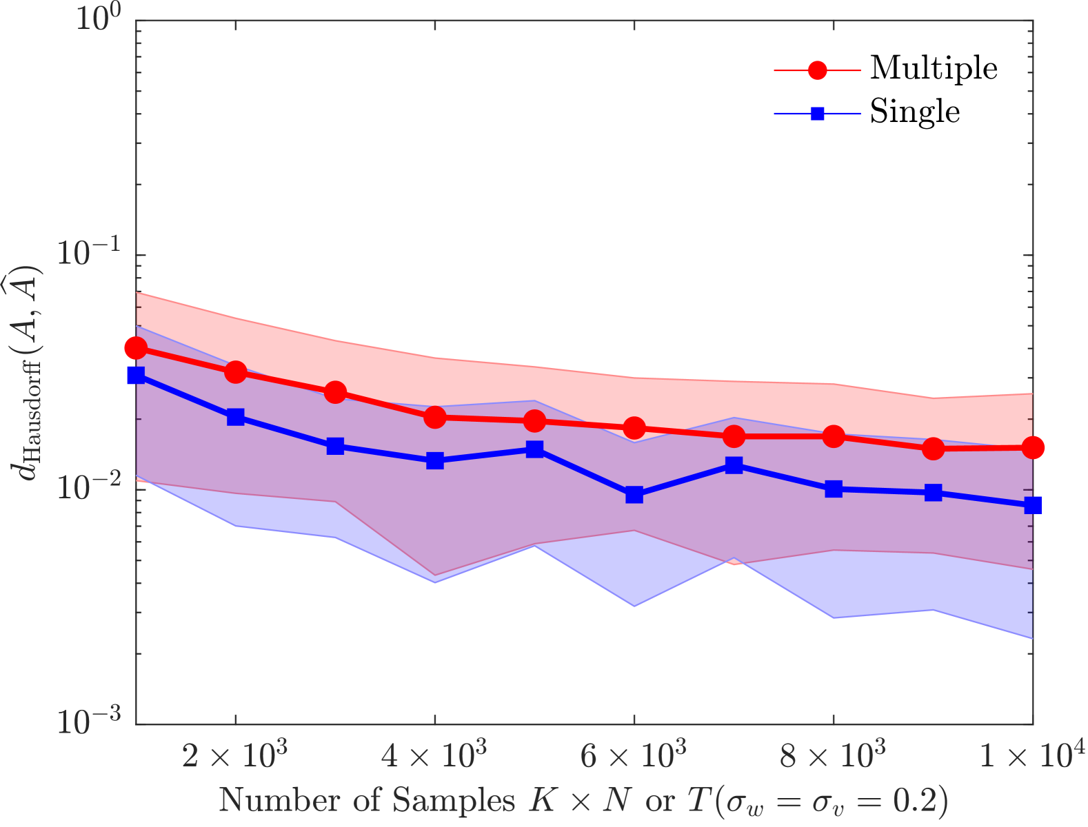
(a)

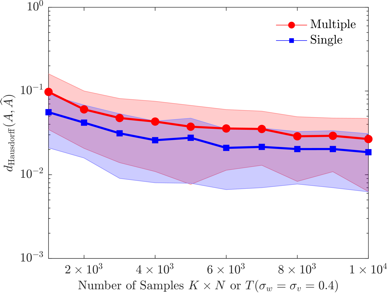
(b)

(c)

(d)

Figure 1: Comparison of system pole estimation errors under different noise levels and sample sizes. In each subplot, the red curve represents the Ho-Kalman algorithm from [30], which utilizes multiple trajectories, while the blue curve corresponds to the Ho-Kalman algorithm from [2], based on a single trajectory.

5 Conclusions

This paper has analyzed the identification errors in system pole estimation for $n$-dimensional discrete-time LTI systems with $m$ outputs and $p$ inputs, using the classical Ho-Kalman algorithm with finite input-output sample data. By establishing non-asymptotic high-probability bounds, we quantify the estimation error under both single-trajectory and multiple-trajectory settings. Our results indicate that the estimation error of system poles decays at a rate of at least $\mathcal{O}\{T^{-\frac{1}{2n}}\}$ when a single trajectory is used and at least $\mathcal{O}\{N^{-\frac{1}{2n}}\}$ when multiple trajectories are available, where $T$ denotes the length of a single trajectory and $N$ represents the number of trajectories. Additionally, we demonstrated that achieving a constant estimation accuracy for system poles requires the sample size to grow super-polynomially with respect to the larger of the two ratios, $\max\{n/m,n/p\}$. Future work involves extending the results to the continuous-time setting.

Appendix

Lemma 2 ([47]).

Given $\mathcal{A}=(\alpha_{ij})\in\mathbb{C}^{n\times n}$, $\mathcal{B}=(\beta_{ij})\in\mathbb{C}^{n\times n}$, suppose that $\lambda(\mathcal{A})=\{\lambda_{1}(\mathcal{A}),\cdots,\lambda_{n}(\mathcal{A})\}$ and $\lambda(\mathcal{B})=\{\mu_{1}(\mathcal{B}),\cdots,\mu_{n}(\mathcal{B})\}$ are the spectra of matrices $\mathcal{A}$ and $\mathcal{B}$ respectively, then the Hausdorff distance between the spectra of matrices $\mathcal{A}$ and $\mathcal{B}$ satisfy

$$d_{\rm H}(\mathcal{A},\mathcal{B})\leq n^{\frac{1}{2n}}\left[\left(1+\frac{1}{\sqrt{n}}\right)^{n}-1\right]^{\frac{1}{n}}m_{\rm F}^{1-\frac{1}{n}}\|\mathcal{A}-\mathcal{B}\|_{\rm F}^{\frac{1}{n}},$$ (45)

where $m_{\rm F}=\max\{\|\mathcal{A}\|_{\rm F},\|\mathcal{B}\|_{\rm F}\}$.

This lemma indicates that the Hausdorff distance between the spectra of matrices $\mathcal{A}$ and $\mathcal{B}$ can be controlled by the distance between matrices $\mathcal{A}$ and $\mathcal{B}$ in the sense of matrix norm.

Lemma 3 ([2]).

The Hankel matrices $H$, $\widehat{H}$, and $L$, $\widehat{L}$ defined in Subsection 2.2, satisfy the following perturbation conditions:

$$\max\left\{\|H^{+}-\widehat{H}^{+}\|,\|H^{-}-\widehat{H}^{-}\|\right\}\leq\|H-\widehat{H}\|\leq\sqrt{\min\{K_{1},K_{2}+1\}}\|G-\widehat{G}\|,$$ (46)

$$\|L-\widehat{L}\|\leq 2\|H^{-}-\widehat{H}^{-}\|\leq 2\sqrt{\min\{K_{1},K_{2}\}}\|G-\widehat{G}\|.$$ (47)

Theorem 6 ([2]).

For the system (2), under the conditions of Assumption 1 and 2, let $H$ and $\widehat{H}$ be the Hankel matrices constructed from the Markov parameter matrices $G$ and $\widehat{G}$ with multiple sample trajectories $\{(u_{k}^{(i)},y_{k}^{(i)}):0\leq k\leq K-1,1\leq i\leq N\}$, respectively, via (13). Let $\overline{A},\overline{B},\overline{C},\overline{D}$ be the the state-space realization corresponding to the output of Ho–Kalman algorithm with input $G$ and $\widehat{A},\widehat{B},\widehat{C},\widehat{D}$ be the state-space realization corresponding to output of Ho-Kalman algorithm with input $\widehat{G}$. Suppose $\sigma_{n}(L)>0$ and perturbation obeys

$$\|L-\widehat{L}\|\leq\frac{\sigma_{n}(L)}{2}.$$ (48)

Then there exists a unitary matrix $\mathcal{U}\in\mathbb{R}^{n\times n}$ such that

$$\|\overline{A}-\mathcal{U}^{\top}\widehat{A}\mathcal{U}\|_{\rm F}\leq\frac{9\sqrt{n}}{\sigma_{n}(L)}\left(\frac{\|L-\widehat{L}\|}{\sigma_{n}(L)}\|H^{+}\|+\|H^{+}-\widehat{H}^{+}\|\right).$$ (49)

References

- [1] L. Ljung, “System identification: theory for the user prentice-hall, inc,” Upper Saddle River, NJ, USA, 1986.
- [2] S. Oymak and N. Ozay, “Revisiting ho–kalman-based system identification: Robustness and finite-sample analysis,” IEEE Transactions on Automatic Control, vol. 67, no. 4, pp. 1914–1928, 2021.
- [3] M. Verhaegen and P. Dewilde, “Subspace model identification part 1. the output-error state-space model identification class of algorithms,” International Journal of Control, vol. 56, no. 5, pp. 1187–1210, 1992.
- [4] D. A. Kodde, F. Plam, and G. A. Pfann, “Asymptotic least-squares estimation efficiency considerations and applications,” Journal of Applied Econometrics, vol. 5, no. 3, pp. 229–243, 1990.
- [5] J. S. Gibson, G. Lee, and C.-F. Wu, “Least-squares estimation of input/output models for distributed linear systems in the presence of noise,” Automatica, vol. 36, no. 10, pp. 1427–1442, 2000.
- [6] M. Deistler, K. Peternell, and W. Scherrer, “Consistency and relative efficiency of subspace methods,” Automatica, vol. 31, no. 12, pp. 1865–1875, 1995.
- [7] M. Viberg, B. Wahlberg, and B. Ottersten, “Analysis of state space system identification methods based on instrumental variables and subspace fitting,” Automatica, vol. 33, no. 9, pp. 1603–1616, 1997.
- [8] G. C. Goodwin and R. L. Payne, DYNAMIC SYSTEM IDENTIFICATION. Elsevier, 1977. [Online]. Available: https://www.sciencedirect.com/science/article/pii/S0076539208632270
- [9] S. J. Qin, “An overview of subspace identification,” Computers & chemical engineering, vol. 30, no. 10-12, pp. 1502–1513, 2006.
- [10] M. Jansson and B. Wahlberg, “On consistency of subspace methods for system identification,” Automatica, vol. 34, no. 12, pp. 1507–1519, 1998.
- [11] K. D. West, “Asymptotic normality, when regressors have a unit root,” Econometrica: Journal of the Econometric Society, pp. 1397–1417, 1988.
- [12] M. Jansson, “Asymptotic variance analysis of subspace identification methods,” IFAC Proceedings Volumes, vol. 33, no. 15, pp. 91–96, 2000.
- [13] S. Dean, H. Mania, N. Matni, B. Recht, and S. Tu, “On the sample complexity of the linear quadratic regulator,” Foundations of Computational Mathematics, vol. 20, no. 4, pp. 633–679, 2020.
- [14] N. Matni and S. Tu, “A tutorial on concentration bounds for system identification,” in 2019 IEEE 58th Conference on Decision and Control (CDC). IEEE, 2019, pp. 3741–3749.
- [15] N. Matni, A. Proutiere, A. Rantzer, and S. Tu, “From self-tuning regulators to reinforcement learning and back again,” in 2019 IEEE 58th Conference on Decision and Control (CDC). IEEE, 2019, pp. 3724–3740.
- [16] R. Vershynin, High-dimensional probability: An introduction with applications in data science. Cambridge university press, 2018, vol. 47.
- [17] M. J. Wainwright, High-dimensional statistics: A non-asymptotic viewpoint. Cambridge university press, 2019, vol. 48.
- [18] M. K. S. Faradonbeh, A. Tewari, and G. Michailidis, “Finite time identification in unstable linear systems,” Automatica, vol. 96, pp. 342–353, 2018.
- [19] M. Simchowitz, H. Mania, S. Tu, M. I. Jordan, and B. Recht, “Learning without mixing: Towards a sharp analysis of linear system identification,” in Conference On Learning Theory. PMLR, 2018, pp. 439–473.
- [20] M. Simchowitz, R. Boczar, and B. Recht, “Learning linear dynamical systems with semi-parametric least squares,” in Conference on Learning Theory. PMLR, 2019, pp. 2714–2802.
- [21] T. Sarkar and A. Rakhlin, “Near optimal finite time identification of arbitrary linear dynamical systems,” in International Conference on Machine Learning. PMLR, 2019, pp. 5610–5618.
- [22] A. Tsiamis and G. J. Pappas, “Finite sample analysis of stochastic system identification,” in 2019 IEEE 58th Conference on Decision and Control (CDC). IEEE, 2019, pp. 3648–3654.
- [23] ——, “Linear systems can be hard to learn,” in 2021 60th IEEE Conference on Decision and Control (CDC). IEEE, 2021, pp. 2903–2910.
- [24] A. Tsiamis, I. M. Ziemann, M. Morari, N. Matni, and G. J. Pappas, “Learning to control linear systems can be hard,” in Conference on Learning Theory. PMLR, 2022, pp. 3820–3857.
- [25] A. Tsiamis and G. J. Pappas, “Online learning of the kalman filter with logarithmic regret,” IEEE Transactions on Automatic Control, vol. 68, no. 5, pp. 2774–2789, 2022.
- [26] Y. Jedra and A. Proutiere, “Sample complexity lower bounds for linear system identification,” in 2019 IEEE 58th Conference on Decision and Control (CDC). IEEE, 2019, pp. 2676–2681.
- [27] ——, “Finite-time identification of stable linear systems optimality of the least-squares estimator,” in 2020 59th IEEE Conference on Decision and Control (CDC). IEEE, 2020, pp. 996–1001.
- [28] ——, “Finite-time identification of linear systems: Fundamental limits and optimal algorithms,” IEEE Transactions on Automatic Control, vol. 68, no. 5, pp. 2805–2820, 2022.
- [29] Y. Sun, S. Oymak, and M. Fazel, “Finite sample system identification: Optimal rates and the role of regularization,” in Learning for Dynamics and Control. PMLR, 2020, pp. 16–25.
- [30] Y. Zheng and N. Li, “Non-asymptotic identification of linear dynamical systems using multiple trajectories,” IEEE Control Systems Letters, vol. 5, no. 5, pp. 1693–1698, 2020.
- [31] H. Wang and J. Anderson, “Large-scale system identification using a randomized svd,” in 2022 American Control Conference (ACC). IEEE, 2022, pp. 2178–2185.
- [32] J. He, C. R. Rojas, and H. Hjalmarsson, “A weighted least-squares method for non-asymptotic identification of markov parameters from multiple trajectories,” IFAC-PapersOnLine, vol. 58, no. 15, pp. 169–174, 2024.
- [33] N. Chatzikiriakos and A. Iannelli, “Sample complexity bounds for linear system identification from a finite set,” IEEE Control Systems Letters, 2024.
- [34] A. Wagenmaker and K. Jamieson, “Active learning for identification of linear dynamical systems,” in Conference on Learning Theory. PMLR, 2020, pp. 3487–3582.
- [35] S. Sun, “Non-asymptotic analysis of subspace identification for stochastic systems using multiple trajectories,” arXiv preprint arXiv:2501.18853, 2025.
- [36] A. Tsiamis, I. Ziemann, N. Matni, and G. J. Pappas, “Statistical learning theory for control: A finite-sample perspective,” IEEE Control Systems Magazine, vol. 43, no. 6, pp. 67–97, 2023.
- [37] Y. Zheng, L. Furieri, M. Kamgarpour, and N. Li, “Sample complexity of linear quadratic gaussian (lqg) control for output feedback systems,” in Learning for Dynamics and Control. PMLR, 2021, pp. 559–570.
- [38] S. Lale, K. Azizzadenesheli, B. Hassibi, and A. Anandkumar, “Logarithmic regret bound in partially observable linear dynamical systems,” Advances in Neural Information Processing Systems, vol. 33, pp. 20 876–20 888, 2020.
- [39] M. Hardt, T. Ma, and B. Recht, “Gradient descent learns linear dynamical systems,” Journal of Machine Learning Research, vol. 19, no. 29, pp. 1–44, 2018.
- [40] F. Brasch and J. Pearson, “Pole placement using dynamic compensators,” IEEE Transactions on Automatic Control, vol. 15, no. 1, pp. 34–43, 1970.
- [41] G. Papageorgiou and K. Glover, “H-infinity loop shaping-why is it a sensible procedure for designing robust flight controllers?” in Guidance, Navigation, and Control Conference and Exhibit, 1999, p. 4272.
- [42] W. R. Evans, “Control system synthesis by root locus method,” Transactions of the American Institute of Electrical Engineers, vol. 69, no. 1, pp. 66–69, 1950.
- [43] B. Ho and R. E. Kálmán, “Effective construction of linear state-variable models from input/output functions,” at-Automatisierungstechnik, vol. 14, no. 1-12, pp. 545–548, 1966.
- [44] F. Hausdorff, Grundzüge der mengenlehre. von Veit, 1914, vol. 7.
- [45] S. Sun, J. Li, and Y. Mo, “Finite time performance analysis of mimo systems identification,” 2023. [Online]. Available: https://arxiv.org/abs/2310.11790
- [46] Y. Zheng and N. Li, “Non-asymptotic identification of linear dynamical systems using multiple trajectories,” arXiv preprint arXiv:2009.00739, 2020.
- [47] S. Sun, “Non-asymptotic error analysis of subspace identification for deterministic systems,” arXiv preprint arXiv:2412.16761, 2024.