Natural inflation in Palatini $F(R,X)$

Abstract

In the context of Palatini gravity, $F(R,X)$ models, with X the inflaton kinetic term, are characterized by the appealing property of generating asymptotically flat inflaton potentials. In this paper, we study the case of a Jordan frame potential which is positive and bounded, specifically, natural inflation. We compute the CMB observables and show that for a wide class of $F(R,X)$ theories, including the quadratic one, natural inflation is still viable.

1 Introduction

As observations of cosmic microwave background radiation (CMB) demonstrate, our universe is flat and homogeneous at large scales. By introducing an accelerated period of expansion in the early universe before the hot big bang, it is possible to generate the observed flatness and homogeneity without fine-tuning of initial conditions [1, 2, 3, 4]. This period of accelerated expansions is called inflation. In the simplest version, inflation is driven by the quasi-constant energy density of the inflaton, a scalar particle embedded in General Relativity (GR). However, most of the simplest models are strongly disfavored by the current CMB measurements [5, 6]. Among such models there is natural inflation, first introduced in [7], which naturally solves the fine-tuning problem of the inflaton potential. There have been several attempts in order to restore its viability (e.g. [8, 9, 10, 11, 12, 13, 14, 15, 16, 17, 18, 19, 20, 21] and refs. therein). Notably several of them rely on non-minimal formulations of gravity, as they give more freedom in formulating the theory and exploring the available parameter space (e.g. [22, 23] and refs. therein). Among them, non-minimally coupled to gravity models in the Palatini formulation have received a lot of attention recently, e.g. [24, 25, 26, 27, 28, 29, 30, 31, 32, 33, 34, 35, 36, 37, 38, 39, 40, 41, 42, 43, 44, 45, 46, 47, 48, 49, 50, 51, 52, 53, 54, 55, 56, 57, 58, 59, 60, 61, 62, 63, 64, 65, 66, 67, 68, 69, 70, 71, 72, 73, 74, 75, 76]. In the metric formulation, the only dynamical degree of freedom is the metric, and the affine connection is assumed to be the Levi-Civita one. On the other hand, in the case of Palatini gravity, the affine connection and the metric tensor are considered a priori independent, and the relation between them is set by the corresponding equations of motion (EOMs). The two formulations have been proved to be equivalent in the case of minimally coupled gravity. However, in presence of non-minimal theories of gravity, the two formulations are not equivalent anymore and yield different phenomenological predictions [77, 78].

In this study, we are interested in a particular class of non-minimal Palatini models: the $F(R,X)$ models, with $X$ the inflaton kinetic term. This kind of theories has been introduced in [79] as way to heal the Palatini $F(R)_{>2}$ (that is those containing terms diverging faster than $R^{2}$) class of models, which has shown to have dynamical issues with the evolution of the scalar field outside slow-roll due, to the presence of higher-order kinetic terms in the Einstein frame. The remarkable feature of this class of theories is the positivity of Einstein frame inflaton potential, regardless of the initial sign of the Jordan frame one [76]. Therefore, in this context, inflation has been extensively studied in [79, 80] for both positive and negative unbounded inflaton potentials in the Jordan frame, as an extended generalization of the $F(R)$ models already explored in [76]. Moreover $F(R,X)$ models seems to provide a natural framework for quintessential inflation realizations [79, 80, 81].

The main purpose of this manuscript is to study the remaining complementary case, that is a positive bounded potential in the Jordan frame embedded in $F(R,X)$ Palatini gravity. In particular, we choose the case of natural inflation. The paper is organized as follows. In section 2, we introduce the class of Palatini $F(R,X)$ models, and describe their fundamental features. In section 3, we compute the CMB observables for $F(R,X)_{\leq 2}$ while in section 4 we do the same but for the $F(R,X)_{>2}$ case. In section 5, we summarize the results and draw our conclusion. Finally, some additional details about slow-roll computation are given in Appendix A.

2 Palatini $F(R,X)$ theories

In the following, we assume Planck units, where $M_{\text{P}}$ is set equal to unity, and a space-like metric signature. The starting point for the $F(R,X)$ action has the form:

$$S_{J}=\int\differential^{4}x\sqrt{-g_{J}}\left[\frac{1}{2}F(R(\Gamma),X)-V(\phi)\right]\,,$$ (2.1)

where $X$ is the inflaton kinetic term given by $X\equiv-g_{J}^{\mu\nu}\partial_{\mu}\phi\partial_{\nu}\phi$, where the use of the Palatini formulation of gravity (and therefore an independent affine connection $\Gamma^{\rho}_{\mu\nu}$) is emphasized in the notation “$R(\Gamma)$” for the curvature scalar. In this work, we follow the simplest case for which $F(R,X)=F(R_{X})$ with $R_{X}\equiv R+X$. This generic setup has been extensively studied in [80, 79, 81], therefore we summarize in the following only the most important details. By introducing an auxiliary field $\zeta$, we can rewrite the action as:

$$S_{J} = \int\differential^{4}x\sqrt{-g}_{J}\left[\frac{1}{2}\left[F(\zeta)+F^{\prime}(\zeta)\left(R_{X}-\zeta\right)\right]-V(\phi)\right]\,,$$ (2.2)

where we used $F^{\prime}(\zeta)\equiv\partial F/\partial\zeta$. By performing a Weyl transformation we can move to the Einstein frame,

$$g_{E\,\mu\nu}=F^{\prime}(\zeta)\ g_{J\,\mu\nu}\,,$$ (2.3)

which gives

$$S_{E}=\int\differential^{4}x\sqrt{-g_{E}}\left[\frac{1}{2}R_{E}-\frac{1}{2}g_{E}^{\mu\nu}\partial_{\mu}\phi\partial_{\nu}\phi-U(\phi,\zeta)\right]\,,$$ (2.4)

where we notice that the canonically normalized scalar field $\phi$ is the same that appeared in the Jordan frame inside the argument of the $F$ function. The scalar field potential takes the form:

$$U(\phi,\zeta)=\frac{V(\phi)}{F^{\prime}(\zeta)^{2}}-\frac{F(\zeta)}{2F^{\prime}(\zeta)^{2}}+\frac{\zeta}{2F^{\prime}(\zeta)}\,.$$ (2.5)

By varying (2.4) with respect to $\zeta$, we get its EOM in the Einstein frame,

$$G(\zeta)=V(\phi)\,,$$ (2.6)

with

$$G(\zeta)\equiv\frac{1}{4}[2F(\zeta)-\zeta F^{\prime}(\zeta)].$$ (2.7)

Applying the computational strategy introduced in [76], one can show that the Einstein frame inflaton potential can be formally written as a function of $\zeta$ only:

$$U(\zeta)=\frac{1}{4}\frac{\zeta}{F^{\prime}(\zeta)}\,.$$ (2.8)

In general, (2.6) can’t be solved explicitly for $\zeta$, however, we can still compute the CMB observables by using the formalism developed in [76] i.e. using $\zeta$ as the computational variable. Consistency of the theory requires $F^{\prime}(\zeta)>0$. If this constraint is satisfied and $\zeta$ is positive, then $U$ is positive definite for any $V(\phi)$, positive or negative, that satisfies eq. (2.6). The case of a positive $V(\phi)$ and unbounded from above and of a negative $V(\phi$) unbounded from below have been already studied in [80, 79]. This time we study the complementary case in which $V(\phi)$ is positive and bounded from above. Specifically, we study the case of a Jordan frame potential given by natural inflation:

$$V(\phi)=\Lambda^{4}\left[1+\cos{\left(\frac{\phi}{M}\right)}\right].$$ (2.9)

In the following, we consider polynomial $F$ of the form

$$F(\zeta)=\zeta+\alpha\zeta^{n}\,,$$ (2.10)

and study separately $n\leq 2$ and $n>2$ because of the different properties that $G(\zeta)$ will exhibit when studying the two distinct cases.

3 Natural inflation for $n\leq 2$

The function $G(\zeta)$, obtained from a $F(\zeta)$ given by eq. (2.10), reads

$$G(\zeta)=\frac{1}{4}(\zeta+\alpha(2-n)\zeta^{n}).$$ (3.1)

It is then clear that the function is positive and monotonically increasing for any $\zeta>0$ and $1<n\leq 2$. This ensures that the mapping between $G(\zeta)$ and $V(\phi)$ is always possible and, in particular, for $n=2$ it allows to solve explicitly (2.6), giving $\zeta=4V(\phi)$. We also stress that the passage from $n\neq 2$ to $n=2$ is discontinuous because of the appearance (disappearance) of the $(2-n)\zeta^{n}$ contribution when $n\neq 2$ $(n=2)$. We will start from the latter, given the simplicity of the computations, and then study and compute the CMB observables for $1<n<2$ (in particular $n=\frac{3}{2},\frac{7}{4}$ in order to understand the behavior as $n\rightarrow 2$).

For the $n=2$ case, the Einstein frame potential can be explicitly written as:

$$U(\phi)=\frac{\Lambda^{4}\quantity(1+\cos\frac{\phi}{M})}{1+8\alpha\Lambda^{4}\quantity(1+\cos\frac{\phi}{M})}.$$ (3.2)

We show an indicative plot of the potential in Fig. 1 for the choice $M=5$, and $\alpha=2\cdot 10^{8}$(red), $\alpha=2\cdot 10^{9}$(blue). $\Lambda\sim 5\cdot 10^{-3}$ is fixed by imposing the constraint $A_{s}\simeq 2.1\cdot 10^{-9}$. We also show for reference the field values $\phi_{N}$ and $\phi_{end}$, respectively corresponding to the “beginning” and “end of inflation”. As $\alpha$ increases, the height of the plateaus decreases, and their width becomes much larger than the width of the minima of the potential where the field will perform reheating. The potential is periodic with period $2\pi M$.

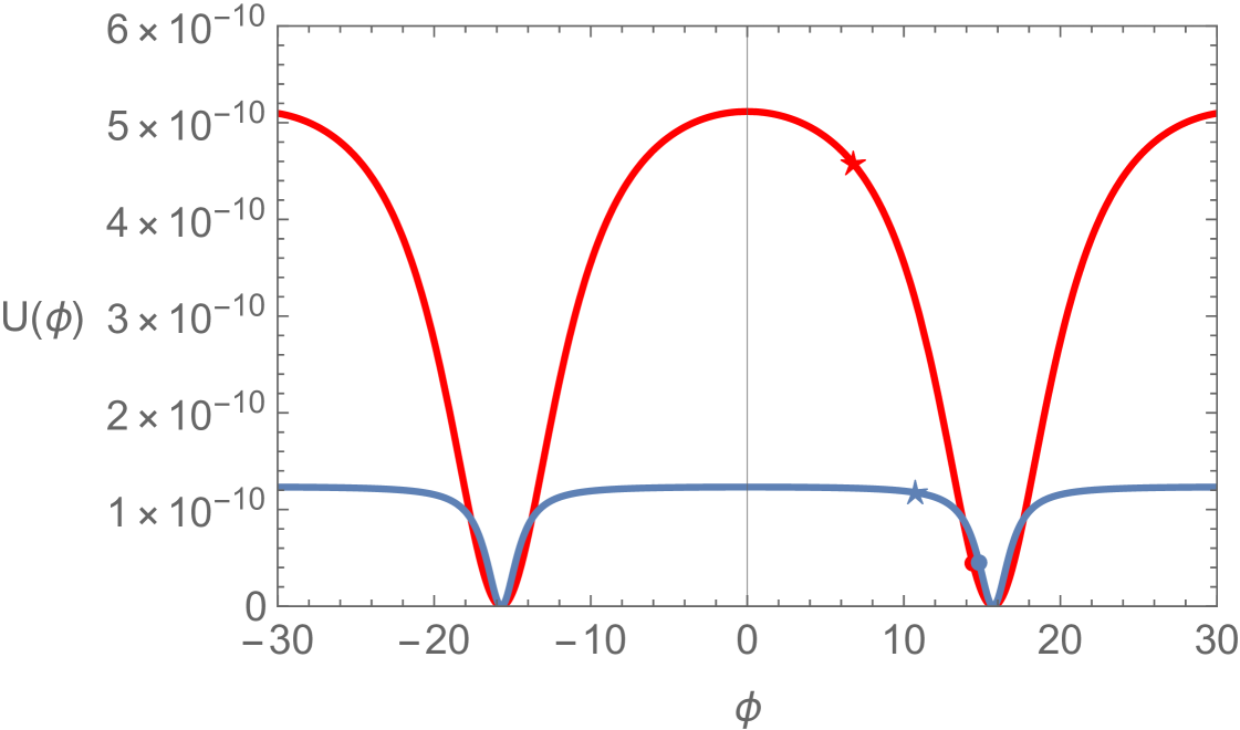
Figure 1: Einstein frame potential for the quadratic $F(R_{X})=R_{X}+\alpha R_{X}^{2}$ with $M=5$, and $\alpha=2\cdot 10^{8}$ (red), $\alpha=10^{9}$ (blue), $\Lambda\sim 5\cdot 10^{-3}$ is fixed by imposing the constraint $A_{s}\simeq 2.1\cdot 10^{-9}$. We also show for reference the field values $\phi_{N}$ (star) and $\phi_{end}$ (dot). As $\alpha$ increases, the width of the plateaus becomes much larger than the width of the minima of the potential where the field will perform reheating.

We now proceed with the evaluation of the slow-roll parameters for the case $n=2$:

$$\epsilon(\phi_{N}) = \frac{\tan^{2}\quantity(\frac{\phi_{N}}{2M})}{2M^{2}\quantity(8\alpha\Lambda^{4}+8\alpha\Lambda^{4}\cos(\frac{\phi_{N}}{M})+1)^{2}},$$ (3.3)

$$\eta(\phi_{N}) = \frac{4\alpha\Lambda^{4}\left(\cos\left(\frac{2\phi_{N}}{M}\right)-3\right)-\left(8\alpha\Lambda^{4}+1\right)\cos\left(\frac{\phi_{N}}{M}\right)}{M^{2}\left(\cos\left(\frac{\phi_{N}}{M}\right)+1\right)\left(8\alpha\Lambda^{4}+8\alpha\Lambda^{4}\cos\left(\frac{\phi_{N}}{M}\right)+1\right)^{2}},$$ (3.4)

and the number of efolds reads:

$$N_{e}=-2M^{2}\left[4\alpha\Lambda^{4}\cos\left(\frac{\phi}{M}\right)+\left(16\alpha\Lambda^{4}+1\right)\ln\left(\sin\left(\frac{\phi}{2M}\right)\right)\right]_{\phi_{end}}^{\phi_{N}}$$ (3.5)

The corresponding CMB observables are given by:

$$r =16\epsilon(\phi_{N}),$$ (3.6)

$$n_{s} =1+2\eta(\phi_{N})-6\epsilon(\phi_{N}),$$ (3.7)

$$A_{s} =\frac{U(\phi_{N})}{24\pi^{2}\epsilon(\phi_{N})}.$$ (3.8)

It can be proven numerically that by increasing $\alpha$ both ${\phi_{end}}$ and ${\phi_{N}}$ approach $M\pi$ (see also Fig. 1). Therefore, by making an expansion at the leading order around $\phi=M\pi$ we can obtain the following approximated results valid in the strong coupling regime:

$$r \simeq\frac{M}{\sqrt{2}\sqrt{\alpha}\Lambda^{2}N_{e}^{3/2}}\,,$$ (3.9)

$$n_{s} \simeq 1-\frac{3}{2N_{e}}+\frac{M}{2\sqrt{2}\sqrt{\alpha}\Lambda^{2}N_{e}^{3/2}}\,,$$ (3.10)

$$A_{s} \simeq\frac{\Lambda^{2}N_{e}^{3/2}}{6\sqrt{2}\pi^{2}\sqrt{\alpha}M}\,.$$ (3.11)

For the $n<2$ models, we cannot solve (2.6) explicitly hence we have to use the formalism derived in [76], where the auxiliary field $\zeta$ is used as the computational variable. At large $\alpha$, we get the following expressions for the CMB observables (see Appendix (A.5)-(A.10) for the full expressions of the slow-roll parameters and the inflationary observables):

$$r(\zeta_{N}) \approx\frac{8(n-2)^{2}}{M^{2}n^{2}\left(e^{\frac{(2-n)N_{e}}{nM^{2}}}-1\right)},$$ (3.12)

$$n_{s}(\zeta_{N}) \approx 1+\frac{(2-n)}{M^{2}n^{2}}\left(\frac{2}{e^{\frac{(n-2)N_{e}}{M^{2}n}}-1}+2-n\right),$$ (3.13)

$$A_{s}(\zeta_{N}) \approx-\frac{M^{2}2^{\frac{6}{n}-7}n^{2}e^{-\frac{(n-2)N_{e}}{M^{2}n}}}{3\pi^{2}\Lambda^{4}(n-2)}\left(\frac{\Lambda^{4}\left(e^{\frac{(n-2)N_{e}}{M^{2}n}}-1\right)}{\alpha(n-2)}\right)^{2/n}\,.$$ (3.14)

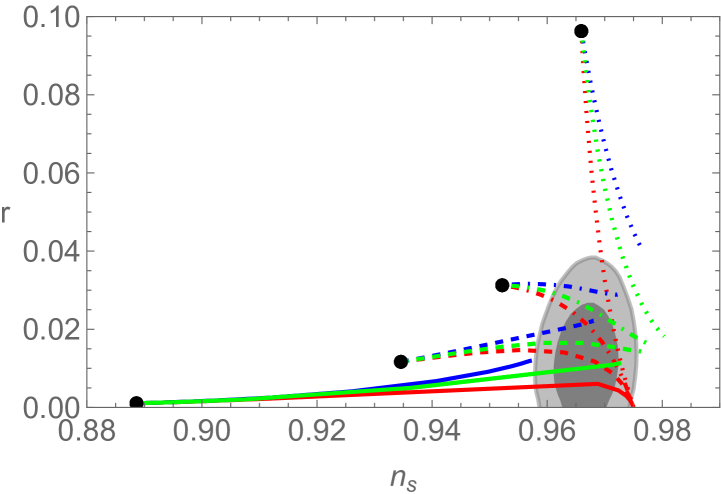
(a)

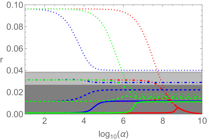
(b)

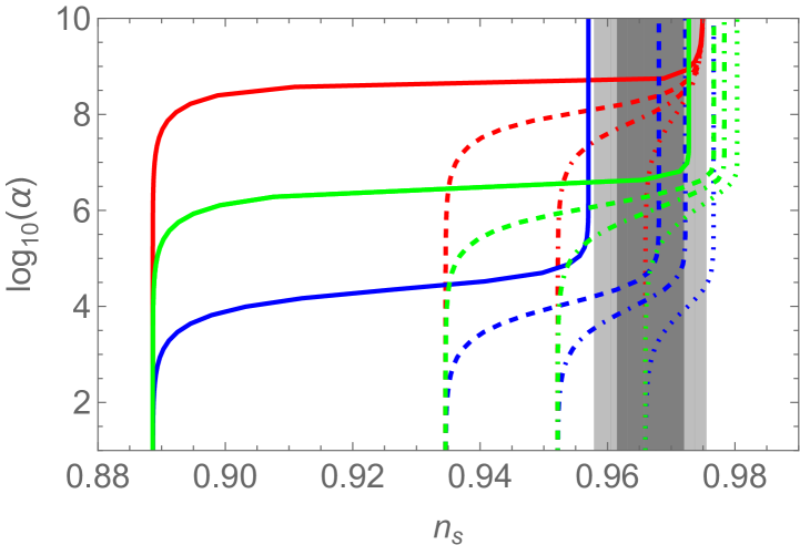
(c)

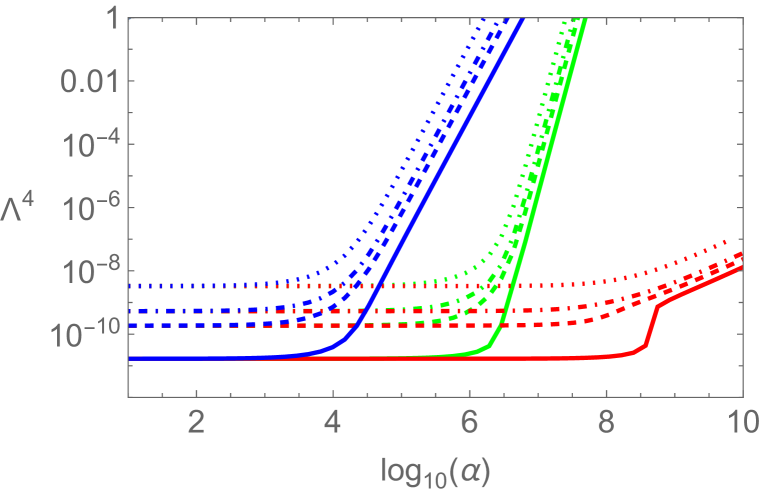
(d)

Figure 2: (a) $r$ vs. $n_{s}$, (b) $r$ vs. $\log_{10}(\alpha)$, (c) $n_{s}$ vs. $\log_{10}(\alpha)$, and (d) $\Lambda^{4}$ vs. $\log_{10}(\alpha)$ for the model presented in section 3, with $n=3/2$ (blue) $n=7/4$ (green) and $n=2$ (red) with $M=3$ (thick), $M=4$ (dashed), $M=5$ (dash-dotted), and $M=10$ (dotted). The black dots show the predictions of the original natural inflation model. All observables are computed at $N_{e}=60$. The amplitude of the power spectrum $A_{s}$ is fixed to its observed value. The gray regions indicate the 95% (dark-gray) and 68% (light-gray) confidence levels (CL), respectively, based on the latest combination of Planck, BICEP/Keck, and BAO data [6].

The discontinuity from the $n<2$ to the $n=2$ case can be appreciated in eqs. (3.12)-(3.14), where $r$, $n_{s}$ and $A_{s}$ respectively approach 0, 1 and $\infty$ when $n$ approaches 2.

The numerical results for the $n\leq 2$ scenario are shown in Fig. 2 (a) $r$ vs. $n_{s}$, (b) $r$ vs. $\log_{10}(\alpha)$, (c) $n_{s}$ vs. $\log_{10}(\alpha)$, and (d) $\Lambda^{4}$ vs. $\log_{10}(\alpha)$, with $n=3/2$ (blue) $n=7/4$ (green) and $n=2$ (red) with $M=3$ (thick), $M=4$ (dashed), $M=5$ (dash-dotted), and $M=10$ (dotted). The black dots show the predictions of the original natural inflation model. All observables are computed at $N_{e}=60$. The amplitude of the power spectrum $A_{s}$ is fixed to its observed value $A_{s}\sim 2.1\cdot 10^{-9}$ [5]. The gray regions indicate the 95% (dark-gray) and 68% (light-gray) confidence levels (CL), respectively, based on the latest combination of Planck, BICEP/Keck, and BAO data [6].

Panel (a) of Fig. 2 displays the tensor-to-scalar ratio $r$ plotted against the scalar spectral index $n_{s}$. For every choice of $(n,M)$, we scan over $\alpha$ and fix $\Lambda^{4}$ in such a way to have $A_{s}\sim 2.1\cdot 10^{-9}$. The resulting trajectories illustrate how the interplay between the additional $\alpha R_{X}^{n}$ term and the natural inflation potential modifies the prediction for $r$ and $n_{s}$.

Fig. 2 (b) shows the behavior of the tensor-to-scalar ratio $r$ as $\alpha$ varies for three choices of $n$ and $M$, the gray-shaded bands represent projections of the 95% (dark-gray) and 68% (light-gray) confidence levels based on Planck, BICEP/Keck, and BAO data [6]. A key feature is that, for each $n$, increasing $\alpha$ generally drives $r$ towards the allowed regions.

In panel (c) of Fig. 2, we display the scalar spectral index $n_{s}$ against $\log_{10}(\alpha)$ for different choices of $n$ and $M$, while the shaded regions (dark-gray and light-gray) show the projections of the 95% and 68% confidence levels from Planck, BICEP/Keck, and BAO data [6]. In general, we see that, as $\alpha$ increases, the $n_{s}$ value is pushed towards the allowed regions. Different $M$ predict different trajectories for $n_{s}$.

We notice that for the $n=2$ case in the $\alpha\rightarrow\infty$ the trajectories converge to a single point. This can be easily computed taking the corresponding limit in (3.9)-(3.10), obtaining

$$r \sim 0,$$ (3.15)

$$n_{s} \sim 1-\frac{3}{2N_{e}},$$ (3.16)

where the dependence on $M$ disappears, predicting $r=0,n_{s}=0.975$ for $N_{e}=60$, in agreement with Fig. 2. Moreover, the big $\alpha$ limit in eqs. (3.12)-(3.14) for $n<2$ is confirmed as well by the results of Fig. 2.

4 Natural inflation for $n>2$

The computations proceed in the same way as for the $n<2$ case. However, some fundamental differences appear as well. First of all, the asymptotic values of the CMB observables are not anymore given by (3.12)-(3.14), because, as explained in the following, the $\alpha\rightarrow\infty$ regime cannot be achieved. We then use the full expressions presented in the appendix (see (A.5)-(A.10)). However, there are first some important considerations to be done, since as it was shown in [76], the case $n\leq 2$ and $n>2$ are conceptually very different. We see from (3.1) that the function $G(\zeta)$ is positive only between $\zeta=0$ and $\zeta=\zeta_{0}=\quantity(\alpha(n-2))^{1/1-n}$ (i.e. the solution of $G(\zeta)=0$). Moreover $G(\zeta)$ (see Fig. 3) also has a maximum in $\zeta_{\text{max}}$ with

$$\zeta_{\text{max}} =\quantity(\alpha(n-2)n)^{\frac{1}{1-n}},$$ (4.1)

$$G(\zeta_{\text{max}}) =\frac{1}{4}\left(1-\frac{1}{n}\right)(\alpha(n-2)n)^{\frac{1}{1-n}}=\frac{n-1}{4n}\zeta_{\text{max}}.$$ (4.2)

Figure 3: Reference plots of a $G(\zeta)$ (left) generated by a $F_{>2}(R_{X})$ and natural inflation $V(\phi)$ (right). Notice that $G(\zeta)=V(\phi)$ is satisfied easily for any $\phi$ when $\zeta\leq\zeta_{0}$, provided that the local maximum of $G\geq$ is higher than the maximum of $V$.

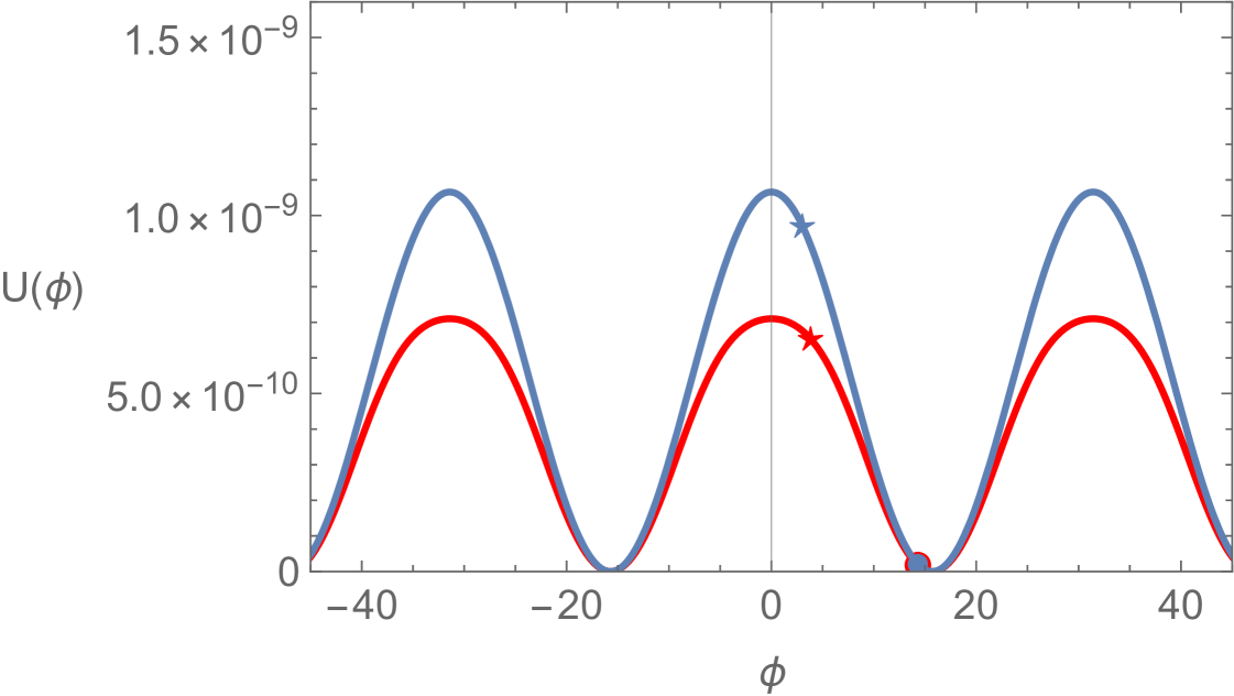
Figure 4: Einstein frame potential for the model $F(R_{X})=R_{X}+\alpha R_{X}^{3}$ with $M=5$, and $\alpha=0$ (i.e. the original natural inflation potential) (blue), and for $\alpha_{max}=1.1\cdot 10^{16}$ (red). We also show for reference the field values $\phi_{N}$ (star) and $\phi_{end}$ (dot). We notice that even for $\alpha=\alpha_{max}$ the potential change is minor. As a consequence, the CMB observables do not change enough, giving $r=0.02,n_{s}=0.957$, still outside the experimental region.

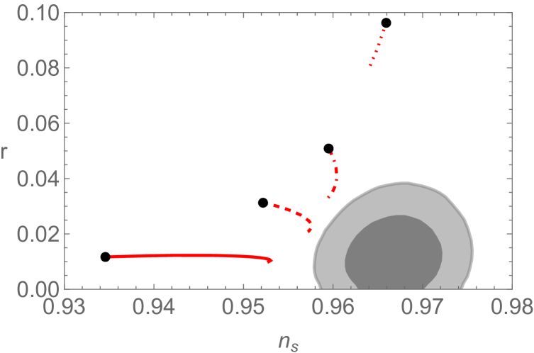
(a)

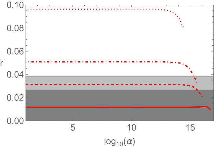
(b)

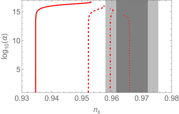
(c)

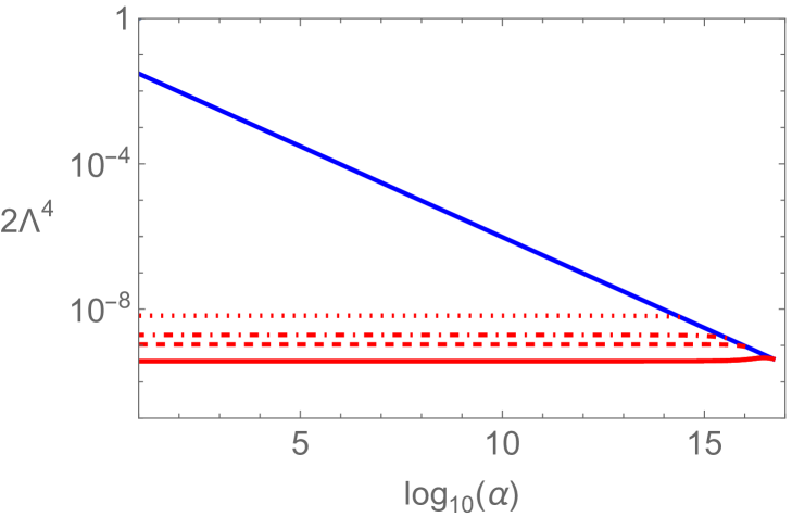
(d)

Figure 5: (a) $r$ vs. $n_{s}$, (b) $r$ vs. $\log_{10}(\alpha)$, (c) $n_{s}$ vs. $\log_{10}(\alpha)$, and (d) $\Lambda$ vs. $\log_{10}(\alpha)$ for the model presented in section 4, with $M=4$ (thick), $M=5$ (dashed), $M=6$ (dashed-dotted), and $M=10$ (dotted) and $n=3$. The black dots show the prediction for the original natural inflation potential. The blue line in (d) is $G(\zeta_{\text{max}})$ as a function of $\alpha$. Notice moreover that we plot $2\Lambda^{4}$, so to make manifest that the model is only defined for $\alpha<\alpha_{max}$. The amplitude of the power spectrum $A_{s}$ is fixed to its observed value. The gray regions indicate the 95% (dark-gray) and 68% (light-gray) confidence levels (CL), respectively, based on the latest combination of Planck, BICEP/Keck, and BAO data [6].

First of all, it is very important to notice that since we want to preserve the validity of eq. (2.6) for all $\phi$ values, we need $G(\zeta_{\text{max}})\geq 2\Lambda^{4}$, that is we want the maximum of the $G(\zeta)$ function to be higher than the maximum of the Jordan frame potential $V(\phi)$. Unfortunately, this cannot always be true since as $\alpha$ increases, $G(\zeta_{\text{max}})$ decreases (see (4.2)).

Therefore, at a given $\Lambda$, $\alpha$ must be smaller (or equal) than a $\Lambda$ dependent $\alpha_{\text{max}}$:

$$\alpha_{\text{max}}=\frac{1}{n(n-2)}\quantity(\frac{n-1}{4n\Lambda})^{n-1}.$$ (4.3)

Therefore, without loss of generality, we start by considering the closest integer number to 2: $n=3$. We show in Fig. 4 the Einstein frame potential for a benchmark point, and in Fig. 5 the numerical results for (a) $r$ vs. $n_{s}$, (b) $r$ vs. $\log_{10}(\alpha)$, (c) $n_{s}$ vs. $\log_{10}(\alpha)$, and (d) $\Lambda$ vs. $\log_{10}(\alpha)$ for the model presented in section 4, with $M=4$ (thick), $M=5$ (dashed), $M=6$ (dashed-dotted), and $M=10$ (dotted) and $n=3$. The black dots show the prediction for the original natural inflation potential. The blue line in (d) is $G(\zeta_{\text{max}})$ as a function of $\alpha$. Notice moreover that we plot $2\Lambda^{4}$ so to make manifest that the model is only defined for $\alpha\leq\alpha_{\text{max}}$ (i.e. for $G(\zeta_{\text{max}})\geq 2\Lambda^{4}$). The amplitude of the power spectrum $A_{s}$ is fixed to its observed value. The gray regions indicate the 95% (dark-gray) and 68% (light-gray) confidence levels (CL), respectively, based on the latest combination of Planck, BICEP/Keck, and BAO data [6]. Since $\alpha$ can’t increase to $\alpha\rightarrow\infty$, the predictions do improve with respect to the original natural inflation potential but not enough to reach the allowed region. This feature is actually shared between all the possible $F(R_{X})_{>2}$ theories. As can be seen from eq. (4.3), the closer $n$ to 2, the higher $\alpha_{\text{max}}$. Therefore we can consider the case in which $n=2+\delta$ with $\delta$ a small effective positive correction induced by a generic $F(R_{X})_{>2}$ in the proximity of $\zeta_{\text{max}}$. In this case (3.1) is given by:

$$G(\zeta)=\frac{1}{4}\zeta\quantity(1-\alpha\delta\zeta^{1+\delta})$$ (4.4)

while,

$$\zeta_{\text{max}}=\quantity(\frac{1}{2\alpha\delta(2+\delta)})^{1/1+\delta}\,.$$ (4.5)

In the limit for $\delta\rightarrow 0$ we get:

$$G(\zeta_{\text{max}})\simeq\frac{1}{16\alpha\delta}.$$ (4.6)

Hence, in order to counterbalance the high $\alpha$ suppression of the $G(\zeta_{\text{max}})$ value, we would need an unnatural $\delta\lesssim\frac{1}{\alpha}$. Therefore, unless ad hoc constructed cases, the $F(R_{X})_{>2}$ framework cannot rescue the natural inflation scenario.

5 Conclusions

We studied the case of natural inflation in the context of Palatini $F(R,X)$ theories. We considered the $F(R,X)$ dependence to take the simple form $F(R,X)=F(R+X)\equiv F(R_{X})$. We then considered two different classes of theories, those with an $R_{X}$ term diverging faster than quadratic and those which diverge slower. The $n<2$ studied cases have shown to improve the results of standard natural inflation. This especially happens for choice of parameter $3\leq M\leq 5$ and for large enough values of $\alpha$, i.e. when the higher order term, $\alpha R_{X}^{n}$, becomes relevant during inflation. On the other hand, when $n=2$, the predictions for any $M$ value appear to enter the 2$\sigma$ allowed region for big enough $\alpha$. However, this cannot be achieved for $F(R_{X})$ that diverges faster than the quadratic case. If we consider the observed $A_{s}$, the relation between the higher-order coupling $\alpha$ and the $\Lambda^{4}$ scale is constrained in such a way that $\alpha$ can never be big enough to contribute to inflation in a sufficient way. In other words, the Einstein frame potential is not substantially modified, and the higher order term represents just an insufficient correction for the prediction of the CMB observables. Summarizing, $F(R_{X})_{\leq 2}$ theories appear to restore the viability of natural inflation and the forthcoming CMB experiments, with a precision of $\delta r\sim 10^{-3}$, such as Simons Observatory [82], CMB-S4 [83] and LITEBIRD [84], will be capable test our scenario, specially for the configurations away from the $r\sim 0$ limit.

Appendix A More details about slow-roll computations

If the Einstein frame potential can be written in terms of the canonical scalar field ($\phi$), by using slow-roll parameters, inflationary predictions can be acquired. The slow-roll parameters with regard to $\phi$ are as follows:

$$\epsilon(\phi)=\frac{1}{2}\left(\frac{U(\phi)^{\prime}}{U(\phi)}\right)^{2}\,,\quad\eta(\phi)=\frac{U(\phi)^{{}^{\prime\prime}}}{U(\phi)}\,,$$ (A.1)

here the superscripts ^′ indicate derivatives with respect to the argument, and it is worth emphasizing that we are setting $M_{P}$ to unity. In the slow-roll approximation, the inflationary parameters can be defined in the form:

$$n_{s}=1-6\epsilon(\phi_{N})+2\eta(\phi_{N})\,,\quad r=16\epsilon(\phi_{N})\,.$$ (A.2)

where $\phi_{N}$ is determined by inverting the equation for the number of e-folds which, in the slow-roll approximation, reads

$$N_{e}=\int^{\phi_{N}}_{\phi_{end}}\frac{U(\phi)}{U(\phi)^{{}^{\prime}}}d\phi\,.$$ (A.3)

where $\phi_{\text{end}}$ is the value of the inflaton, where the inflation halts. It can be computed by using the expression, $\epsilon(\phi_{\text{end}})=1$. The number of e-folds is usually taken around 50-60. Moreover, the amplitude of curvature perturbations in terms of $\phi$ can be expressed by using the form

$$A_{s}=\frac{1}{24\pi^{2}}\frac{U(\phi_{N})}{\epsilon(\phi_{N})}$$ (A.4)

which should be matched with $A_{s}\approx 2.1\times 10^{-9}$ from the Planck results [5] for the pivot scale $k_{N}=0.002$ Mpc^-1.

The full formulas for the slow-roll parameters and CMB observables for $V(\phi)$ given by eq. (2.9) and $F(R)=R+\alpha R^{n}$ can be easily obtained by using the method introduced in [76] i.e. we use $\zeta$ as the computational variable, we write $U$ in terms of $\zeta$ following eq. (2.5) and then compute terms like $U(\phi)^{\prime}$ as $\frac{U(\zeta)^{\prime}}{\phi(\zeta)^{\prime}}$, where $\phi(\zeta)$ is obtained by solving eq. (2.6) in terms of $\phi$. After performing all the computations, the slow-roll parameters read:

$$\epsilon(\zeta_{N}) =\frac{\left(\zeta_{N}+\alpha(2-n)\zeta_{N}^{n}\right)\left(8\Lambda^{4}-\zeta_{N}-\left(\alpha(2-n)\zeta_{N}^{n}\right)\right)}{2M^{2}\left(\zeta_{N}+\alpha n\zeta_{N}^{n}\right)^{2}},$$ (A.5)

$$\eta(\zeta_{N})= \frac{\zeta_{N}^{2}\left(4\Lambda^{4}-\zeta_{N}\right)+\alpha\zeta_{N}^{n+1}\left(\zeta_{N}(n(3n-4)-2)+4\Lambda^{4}n(7-5n)\right)}{M^{2}\left(\zeta_{N}+\alpha n\zeta_{N}^{n}\right)^{2}\left(\zeta_{N}+\alpha(2-n)n\zeta_{N}^{n}\right)}+$$ (A.6)

$$+\frac{(2-n)n\alpha^{2}\zeta_{N}^{2n}\left(\zeta_{N}(4n-7)+4\Lambda^{4}(4-3n)\right)-(2-n)^{3}n\alpha^{3}\zeta_{N}^{3n}}{M^{2}\left(\zeta_{N}+\alpha n\zeta_{N}^{n}\right)^{2}\left(\zeta_{N}+\alpha(2-n)n\zeta_{N}^{n}\right)}.$$

Hence, the number of e-folds is given by:

$$N_{e}=\int_{\zeta_{end}}^{\zeta_{N}}\frac{M^{2}\left(\zeta+\alpha n\zeta^{n}\right)\left(\zeta+\alpha(2-n)n\zeta^{n}\right)}{\zeta\left(\zeta+\alpha(2-n)\zeta^{n}\right)\left(-\zeta+8\Lambda^{4}-\left(\alpha(2-n)\zeta^{n}\right)\right)}d\zeta.$$ (A.7)

and the CMB observables are:

$$r(\zeta_{N}) =16\epsilon(\zeta_{N}),$$ (A.8)

$$n_{s}(\zeta_{N}) =1+2\eta(\zeta_{N})-6\epsilon(\zeta_{N}),$$ (A.9)

$$A_{s}(\zeta_{N}) =\frac{\zeta_{N}^{2}M^{2}\left(\zeta_{N}+\alpha n\zeta_{N}^{n}\right)}{48\pi^{2}\left(\zeta_{N}+\alpha(2-n)\zeta_{N}^{n}\right)\left(-\zeta_{N}+8\Lambda^{4}-\left(\alpha(2-n)\zeta_{N}^{n}\right)\right)}.$$ (A.10)

References

- [1] A. A. Starobinsky, A New Type of Isotropic Cosmological Models Without Singularity, Phys. Lett. B91 (1980) 99.
- [2] A. H. Guth, The Inflationary Universe: A Possible Solution to the Horizon and Flatness Problems, Phys.Rev. D23 (1981) 347.
- [3] A. D. Linde, A New Inflationary Universe Scenario: A Possible Solution of the Horizon, Flatness, Homogeneity, Isotropy and Primordial Monopole Problems, Phys.Lett. B108 (1982) 389.
- [4] A. Albrecht and P. J. Steinhardt, Cosmology for Grand Unified Theories with Radiatively Induced Symmetry Breaking, Phys.Rev.Lett. 48 (1982) 1220.
- [5] Planck collaboration, Planck 2018 results. X. Constraints on inflation, Astron. Astrophys. 641 (2020) A10 [1807.06211].
- [6] BICEP, Keck collaboration, Improved Constraints on Primordial Gravitational Waves using Planck, WMAP, and BICEP/Keck Observations through the 2018 Observing Season, Phys. Rev. Lett. 127 (2021) 151301 [2110.00483].
- [7] K. Freese, J. A. Frieman and A. V. Olinto, Natural inflation with pseudo - Nambu-Goldstone bosons, Phys. Rev. Lett. 65 (1990) 3233.
- [8] A. Achúcarro, V. Atal and Y. Welling, On the viability of and natural inflation, JCAP 07 (2015) 008 [1503.07486].
- [9] R. Z. Ferreira, A. Notari and G. Simeon, Natural Inflation with a periodic non-minimal coupling, JCAP 11 (2018) 021 [1806.05511].
- [10] I. Antoniadis, A. Karam, A. Lykkas, T. Pappas and K. Tamvakis, Rescuing Quartic and Natural Inflation in the Palatini Formalism, JCAP 1903 (2019) 005 [1812.00847].
- [11] A. Salvio, Quasi-Conformal Models and the Early Universe, Eur. Phys. J. C 79 (2019) 750 [1907.00983].
- [12] G. Simeon, Scalar-tensor extension of Natural Inflation, JCAP 07 (2020) 028 [2002.07625].
- [13] E. McDonough, A. H. Guth and D. I. Kaiser, Nonminimal Couplings and the Forgotten Field of Axion Inflation, 2010.04179.
- [14] A. Salvio, Natural-scalaron inflation, JCAP 10 (2021) 011 [2107.03389].
- [15] A. Salvio, BICEP/Keck data and quadratic gravity, JCAP 09 (2022) 027 [2202.00684].
- [16] N. Bostan, Non-minimally coupled Natural Inflation: Palatini and Metric formalism with the recent BICEP/Keck, JCAP 02 (2023) 063 [2209.02434].
- [17] A. Salvio and S. Sciusco, (Multi-field) natural inflation and gravitational waves, JCAP 03 (2024) 018 [2311.00741].
- [18] A. Mukuno and J. Soda, Chromonatural warm inflation, Phys. Rev. D 109 (2024) 123504 [2402.08849].
- [19] A. Racioppi and A. Salvio, Natural metric-affine inflation, JCAP 06 (2024) 033 [2403.18004].
- [20] D. L. Lorenzoni, D. I. Kaiser and E. McDonough, Natural inflation with exponentially small tensor-to-scalar ratio, Phys. Rev. D 110 (2024) L061302 [2405.13881].
- [21] M. Michelotti, R. Gonzalez Quaglia, E. Dimastrogiovanni, M. Fasiello and D. Roest, Kinetic Gauge Friction in Natural Inflation, 2411.19892.
- [22] L. Järv, K. Kannike, L. Marzola, A. Racioppi, M. Raidal, M. Rünkla et al., Frame-Independent Classification of Single-Field Inflationary Models, Phys. Rev. Lett. 118 (2017) 151302 [1612.06863].
- [23] L. Järv, A. Karam, A. Kozak, A. Lykkas, A. Racioppi and M. Saal, Equivalence of inflationary models between the metric and Palatini formulation of scalar-tensor theories, Phys. Rev. D 102 (2020) 044029 [2005.14571].
- [24] N. Tamanini and C. R. Contaldi, Inflationary Perturbations in Palatini Generalised Gravity, Phys. Rev. D83 (2011) 044018 [1010.0689].
- [25] F. Bauer and D. A. Demir, Higgs-Palatini Inflation and Unitarity, Phys. Lett. B698 (2011) 425 [1012.2900].
- [26] S. Rasanen and P. Wahlman, Higgs inflation with loop corrections in the Palatini formulation, JCAP 1711 (2017) 047 [1709.07853].
- [27] T. Tenkanen, Resurrecting Quadratic Inflation with a non-minimal coupling to gravity, JCAP 1712 (2017) 001 [1710.02758].
- [28] A. Racioppi, Coleman-Weinberg linear inflation: metric vs. Palatini formulation, JCAP 1712 (2017) 041 [1710.04853].
- [29] T. Markkanen, T. Tenkanen, V. Vaskonen and H. Veermäe, Quantum corrections to quartic inflation with a non-minimal coupling: metric vs. Palatini, 1712.04874.
- [30] L. Järv, A. Racioppi and T. Tenkanen, The Palatini side of inflationary attractors, 1712.08471.
- [31] A. Racioppi, New universal attractor in nonminimally coupled gravity: Linear inflation, Phys. Rev. D97 (2018) 123514 [1801.08810].
- [32] K. Kannike, A. Kubarski, L. Marzola and A. Racioppi, A minimal model of inflation and dark radiation, Phys. Lett. B792 (2019) 74 [1810.12689].
- [33] V.-M. Enckell, K. Enqvist, S. Rasanen and E. Tomberg, Higgs inflation at the hilltop, JCAP 1806 (2018) 005 [1802.09299].
- [34] V.-M. Enckell, K. Enqvist, S. Rasanen and L.-P. Wahlman, Inflation with term in the Palatini formalism, JCAP 1902 (2019) 022 [1810.05536].
- [35] S. Rasanen, Higgs inflation in the Palatini formulation with kinetic terms for the metric, 1811.09514.
- [36] N. Bostan, Non-minimally coupled quartic inflation with Coleman-Weinberg one-loop corrections in the Palatini formulation, 1907.13235.
- [37] N. Bostan, Quadratic, Higgs and hilltop potentials in the Palatini gravity, 1908.09674.
- [38] P. Carrilho, D. Mulryne, J. Ronayne and T. Tenkanen, Attractor Behaviour in Multifield Inflation, JCAP 1806 (2018) 032 [1804.10489].
- [39] J. P. B. Almeida, N. Bernal, J. Rubio and T. Tenkanen, Hidden Inflaton Dark Matter, JCAP 1903 (2019) 012 [1811.09640].
- [40] T. Takahashi and T. Tenkanen, Towards distinguishing variants of non-minimal inflation, JCAP 1904 (2019) 035 [1812.08492].
- [41] T. Tenkanen, Minimal Higgs inflation with an term in Palatini gravity, Phys. Rev. D99 (2019) 063528 [1901.01794].
- [42] T. Tenkanen and L. Visinelli, Axion dark matter from Higgs inflation with an intermediate , JCAP 1908 (2019) 033 [1906.11837].
- [43] T. Tenkanen, Trans-Planckian Censorship, Inflation and Dark Matter, 1910.00521.
- [44] A. Kozak and A. Borowiec, Palatini frames in scalar-tensor theories of gravity, Eur. Phys. J. C79 (2019) 335 [1808.05598].
- [45] I. Antoniadis, A. Karam, A. Lykkas and K. Tamvakis, Palatini inflation in models with an term, JCAP 1811 (2018) 028 [1810.10418].
- [46] I. D. Gialamas and A. B. Lahanas, Reheating in Palatini inflationary models, 1911.11513.
- [47] A. Racioppi, Non-Minimal (Self-)Running Inflation: Metric vs. Palatini Formulation, JHEP 21 (2020) 011 [1912.10038].
- [48] J. Rubio and E. S. Tomberg, Preheating in Palatini Higgs inflation, JCAP 04 (2019) 021 [1902.10148].
- [49] A. Edery and Y. Nakayama, Palatini formulation of pure gravity yields Einstein gravity with no massless scalar, Phys. Rev. D 99 (2019) 124018 [1902.07876].
- [50] A. Lloyd-Stubbs and J. McDonald, Sub-Planckian inflation in the Palatini formulation of gravity with an term, Phys. Rev. D 101 (2020) 123515 [2002.08324].
- [51] N. Das and S. Panda, Inflation and Reheating in f(R,h) theory formulated in the Palatini formalism, JCAP 05 (2021) 019 [2005.14054].
- [52] J. McDonald, Does Palatini Higgs Inflation Conserve Unitarity?, JCAP 04 (2021) 069 [2007.04111].
- [53] M. Shaposhnikov, A. Shkerin and S. Zell, Quantum Effects in Palatini Higgs Inflation, JCAP 07 (2020) 064 [2002.07105].
- [54] V.-M. Enckell, S. Nurmi, S. Räsänen and E. Tomberg, Critical point Higgs inflation in the Palatini formulation, JHEP 04 (2021) 059 [2012.03660].
- [55] I. D. Gialamas, A. Karam and A. Racioppi, Dynamically induced Planck scale and inflation in the Palatini formulation, JCAP 11 (2020) 014 [2006.09124].
- [56] A. Karam, M. Raidal and E. Tomberg, Gravitational dark matter production in Palatini preheating, JCAP 03 (2021) 064 [2007.03484].
- [57] I. D. Gialamas, A. Karam, A. Lykkas and T. D. Pappas, Palatini-Higgs inflation with nonminimal derivative coupling, Phys. Rev. D 102 (2020) 063522 [2008.06371].
- [58] A. Karam, S. Karamitsos and M. Saal, -function reconstruction of Palatini inflationary attractors, 2103.01182.
- [59] A. Karam, E. Tomberg and H. Veermäe, Tachyonic preheating in Palatini R 2 inflation, JCAP 06 (2021) 023 [2102.02712].
- [60] I. D. Gialamas, A. Karam, T. D. Pappas and V. C. Spanos, Scale-invariant quadratic gravity and inflation in the Palatini formalism, Phys. Rev. D 104 (2021) 023521 [2104.04550].
- [61] J. Annala and S. Rasanen, Inflation with terms in the Palatini formulation, 2106.12422.
- [62] A. Racioppi, J. Rajasalu and K. Selke, Multiple point criticality principle and Coleman-Weinberg inflation, 2109.03238.
- [63] D. Y. Cheong, S. M. Lee and S. C. Park, Reheating in Models with Non-minimal Coupling in metric and Palatini formalisms, 2111.00825.
- [64] Y. Mikura and Y. Tada, On UV-completion of Palatini-Higgs inflation, 2110.03925.
- [65] A. Ito, W. Khater and S. Rasanen, Tree-level unitarity in Higgs inflation in the metric and Palatini formulation, 2111.05621.
- [66] A. Racioppi and M. Vasar, On the number of -folds in the Jordan and Einstein frames, 2111.09677.
- [67] M. AlHallak, A. AlRakik, N. Chamoun and M. S. El-Daher, Palatini f(R) Gravity and Variants of k-/Constant Roll/Warm Inflation within Variation of Strong Coupling Scenario, Universe 8 (2022) 126 [2111.05075].
- [68] M. AlHallak, N. Chamoun and M. S. Eldaher, Natural Inflation with non minimal coupling to gravity in R 2 gravity under the Palatini formalism, JCAP 10 (2022) 001 [2202.01002].
- [69] I. D. Gialamas, A. Karam and T. D. Pappas, Gravitational corrections to electroweak vacuum decay: metric vs. Palatini, 2212.03052.
- [70] K. Dimopoulos, A. Karam, S. Sánchez López and E. Tomberg, Palatini R 2 quintessential inflation, JCAP 10 (2022) 076 [2206.14117].
- [71] K. Dimopoulos, A. Karam, S. Sánchez López and E. Tomberg, Modelling Quintessential Inflation in Palatini-Modified Gravity, Galaxies 10 (2022) 57 [2203.05424].
- [72] I. D. Gialamas and K. Tamvakis, Inflation in Metric-Affine Quadratic Gravity, 2212.09896.
- [73] A. Racioppi, -attractors in metric-affine gravity, 2411.08031.
- [74] I. D. Gialamas and A. Racioppi, Symmetry-breaking inflation in non-minimal metric-affine gravity, 2412.17738.
- [75] N. Bostan and R. H. Dejrah, Minimally coupled -exponential inflation with an term in the Palatini formulation, 2409.10398.
- [76] C. Dioguardi, A. Racioppi and E. Tomberg, Slow-roll inflation in Palatini F(R) gravity, JHEP 06 (2022) 106 [2112.12149].
- [77] T. Koivisto and H. Kurki-Suonio, Cosmological perturbations in the palatini formulation of modified gravity, Class. Quant. Grav. 23 (2006) 2355 [astro-ph/0509422].
- [78] F. Bauer and D. A. Demir, Inflation with Non-Minimal Coupling: Metric versus Palatini Formulations, Phys. Lett. B665 (2008) 222 [0803.2664].
- [79] C. Dioguardi, A. Racioppi and E. Tomberg, Beyond (and back to) Palatini quadratic gravity and inflation, JCAP 03 (2024) 041 [2212.11869].
- [80] C. Dioguardi and A. Racioppi, Palatini : a new framework for inflationary attractors, 2307.02963.
- [81] C. Dioguardi et al., to appear, 25xx.xxxx.
- [82] Simons Observatory collaboration, The Simons Observatory: Science goals and forecasts, JCAP 02 (2019) 056 [1808.07445].
- [83] K. Abazajian et al., CMB-S4 Science Case, Reference Design, and Project Plan, 1907.04473.
- [84] LiteBIRD collaboration, LiteBIRD: JAXA’s new strategic L-class mission for all-sky surveys of cosmic microwave background polarization, Proc. SPIE Int. Soc. Opt. Eng. 11443 (2020) 114432F [2101.12449].