Hamiltonian dynamics of classical spins

Abstract

We discuss the geometry behind classical Heisenberg model at the level suitable for third or fourth year students who did not have the opportunity to take a course on differential geometry. The arguments presented here rely solely on elementary algebraic concepts such as vectors, dual vectors and tensors, as well as Hamiltonian equations and Poisson brackets in their simplest form. We derive Poisson brackets for classical spins, along with the corresponding equations of motion for classical Heisenberg model, starting from the geometry of two-sphere, thereby demonstrating the relevance of standard canonical procedure in the case of Heisenberg model.

I Introduction

Before diving into the quantum world, students familiarize themselves with classical physics. This is certainly not because classical physics is more fundamental, but rather knowledge of classical physics can be helpful in understanding counterintuitive quantum phenomena. Indeed, the so-called process of quantization, both in Hamiltonian and Lagrangian formulations, relies on the corresponding classical physical system as a starting point in constructing quantum theory. Examples of this strategy are numerous: the harmonic oscillator is studied as a prime example in classical mechanics with the quantum version being of equal importance. Pauli’s solution to the quantum mechanical hydrogen atom is the direct analog of Kepler problem in classical mechanics [1, 2]. Finally, the prerequisite for learning quantum electrodynamics is the knowledge of Maxwell’s classical theory [3, 2, 4].

An important exception to this rule of studying quantum system after the classical one is fully understood, is the (quantum) Heisenberg model which captures the physics of localized magnetism. In the simplest case of an isotropic ferromagnet with nearest-neighbor interaction, it is defined by the Hamiltonian operator

$$\hat{H}=-\frac{J}{2}\sum_{\bm{n},\bm{\lambda}}\hat{\bm{S}}(\bm{n})\cdot\hat{\bm{S}}(\bm{n}+\bm{\lambda})$$ (1)

where $J>0$ denotes the exchange integral, $\bm{n}$ is the position vector of a site in the lattice, $\{\bm{\lambda}\}$ is the set of vectors connecting each lattice site with its nearest neighbors, $\hat{\bm{S}}(\bm{n})$ is the spin operator corresponding to the lattice site $\bm{n}$ and components of spin operators satisfy equal-time commutation relation (we are dropping temporal coordinate for clarity)

$$\Big{[}\hat{S}_{\alpha}(\bm{n}),\hat{S}_{\beta}(\bm{m})\Big{]}=\mathrm{i}\epsilon_{\alpha\beta\gamma}\Delta(\bm{n}-\bm{m})\hat{S}_{\gamma}(\bm{n}),$$ (2)

where $\Delta(\bm{n}-\bm{m})=1$ only for $\bm{n}=\bm{m}$ and $\Delta(\bm{n}-\bm{m})=0$ in all other cases and $\epsilon_{\alpha\beta\gamma}$ denotes the Levi-Civita symbol. In essence, $\{\hat{S}_{\alpha}(\bm{n})\}$ operators from different sites commute, while those on the same site satisfy standard $\mathfrak{su}(2)$ commutation relations. The Hilbert space for this model consists of tensor products of spin states at all sites [5].

When introducing Heisenberg model in texts for undergraduate students, authors usually start from the exchange interaction and the Dirac Hamiltonian [6, 7], while graduate-level books discuss the Hubbard model and derive the Heisenberg Hamiltonian as an effective model which describes the physics of spin exchange and superexchange [5, 8, 9, 10]. This kind of presentation is, of course, completely reasonable from the point of view of atomic physics. After all, quantum-mechanical properties of electrons are key to our understanding of magnetism. However, it serves an injustice to the corresponding model of classical spins since spin waves (or magnons), as emergent degrees of freedom in a quantum model, are the quantized version of small collective oscillations of classical spins. Likewise, a direct confrontation with quantum many-body Hamiltonian (1) may leave students wondering what happened to the canonical prescription of replacing Poisson brackets with commutators, or how the spin operators suddenly became dynamical degrees of freedom. It turns out that all these issues arise because the underlying phase space for a single classical spin fails to be a Euclidean space – it is the two-sphere ${\rm S}^{2}$ and a full understanding of the classical Heisenberg model requires certain knowledge of tensor analysis on ${\rm S}^{2}$. The problem is that most undergraduates do not take courses on differential geometry. Still, some elements of differential geometry are used in physics courses. For example, introductory texts on quantum field theory describe gauge field strength as curvature [3, 11], while modern introductory texts to general relativity cover many important geometric concepts [12, 13]. It is unfortunate that the classical Heisenberg model does not get the same treatment, giving the fact that students usually possess needed tools acquired on linear algebra and vector calculus courses and that the symplectic form and associate Poisson tensor, which we shall be discussing here, are no more abstract than the curvature or parallel transport along a curve on a manifold. As far as standard textbook treatments are concerned, the classical Heisenberg model remains somewhat mysterious of an object and students are missing a nice opportunity of connecting classical and quantum Heisenberg models in a compelling way.

The paper is not intended as an introduction to symplectic geometry, nor to the theories of classical and quantum Heisenberg models; standard references cover these topics in depth [14, 15, 5]. Instead, it points to frequently omitted geometry of classical Heisenberg spins and its connection and relevance to the quantum model. In the second section we review vectors, dual vectors and tensors, as well as tensor fields, while the symplectic form and the Poison tensor on $\mathbb{R}^{2}$ are introduced in Section III. Generalization of these objects to the case when phase space is two-sphere is given in Section IV, which also contains an example of a simple system defined on the phase space ${\rm S^{2}}$. Finally, the application of these ideas to the case of classical Heisenberg model is given in Section V and an alternative definition of Poisson brackets in terms of the symplectic form is presented in Section VI. Some technical details and notation on symplectic manifolds are collected in Section VII. We set $\hbar=1$ throughout the paper.

II Vectors, dual vectors and tensors

We shall start by recapitulating some basic facts from the theory of vector spaces just to set up notation. Standard references are [16, 17, 18, 19]. We consider only real vector spaces here.

II.1 Vectors and dual vectors

Let $V$ be a vector space of dimension $N$. Each element $X\in V$ can be uniquely represented as $X=X^{i}e_{i}$, where $\{e_{i}\}$ is the set of basis vectors and $X^{i}$ are components of $X$ with respect to this basis. Here, and throughout the paper, we employ the Einstein summation convention so that in all expressions which contain the same letter as a lower and as an upper index, the summation is carried over all the values of index: $1,2,3,...,N$. Real $N$ dimensional vector space is isomorphic to $\mathbb{R}^{N}$, the space of $N-$tuplets of real numbers. By convention, we write these elements as columns. For example, when $N=2$, to each vector $X=X^{1}e_{1}+X^{2}e_{2}$ we ascribe the column

$$\begin{bmatrix}X^{1}\\ X^{2}\\ \end{bmatrix},$$ (3)

which we denote by the same symbol, $X$.

Dual vectors are linear maps from $V$ to real numbers and, as it turns out, they form a vector space of the same dimension $N$. We denote this space by $V^{*}$ and a typical dual vector $\alpha\in V^{*}$ is written as $\alpha=\alpha_{i}e^{*i}$. Here $\{e^{*i}\}$ denotes the dual basis whose elements are defined by their action on the basis elements of $V$, $e^{*i}(e_{j})=\delta^{i}_{j}$. Dual vectors are represented by rows. If $N=2$, we have

$$\alpha=\alpha_{1}e^{*1}+\alpha_{2}e^{*2}\equiv\begin{bmatrix}\alpha_{1}\;\alpha_{2}\end{bmatrix}$$ (4)

so that the action of $\alpha\in V^{*}$ on $X\in V$ can be written as

$$\alpha(X)=\begin{bmatrix}\alpha_{1}\;\alpha_{2}\end{bmatrix}\begin{bmatrix}X^{1}\\ X^{2}\\ \end{bmatrix}=\alpha_{1}X^{1}+\alpha_{2}X^{2}\equiv X(\alpha),$$ (5)

which is just a real number. The last step in the previous equation simply states that vectors could be considered as linear maps on dual vectors. Although we are usually a bit cavalier when it comes to vectors and dual vectors, we must keep in mind that these are different mathematical objects that should be carefully distinguished.

II.2 Tensors

Vectors and dual vectors can be used to construct more complicated objects – tensors. These are multilinear maps (i.e. linear with respect to each argument) which take certain number of dual vectors and vectors to produce a number. Formally, we say that the multilinear map

$${\rm T}:\underbrace{V^{*}\times V^{*}\times\dots\times V^{*}}_{{\rm n}\;\;\rm{copies}}\times\underbrace{V\times V\times\dots\times V}_{{\rm m}\;\;\rm{copies}}\to\mathbb{R},$$ (6)

where $\times$ denotes Cartesian product, is a tensor of type $(\rm n,m)$. We shall restrict ourselves here to tensors of types $(1,1)$, $(0,2)$ and $(2,0)$.

Tensors of various types are naturally expressed in terms of tensor products. Given two dual vectors, $\alpha,\beta\in V^{*}$, we define their tensor product $\alpha\otimes\beta$ by

$$\alpha\otimes\beta(X,Y):=\alpha(X)\beta(Y),$$ (7)

where $X,Y\in V$. As dual vectors are linear maps, this construction automatically satisfies the definition of a $(0,2)$ type tensor. In terms of its components ${\rm T}_{ij}$, an arbitrary $(0,2)$ type tensor is written as ${\rm T}={\rm T}_{ij}e^{*i}\otimes e^{*j}$, where ${\rm T}_{ij}={\rm T}(e_{i},e_{j})$. In complete analogy, $(2,0)$ and $(1,1)$ tensors are given by ${\rm A}={\rm A}^{ij}e_{i}\otimes e_{j}$ and ${\rm B}={\rm B}^{i}_{\;j}e_{i}\otimes e^{*j}$, with components given by ${\rm A}^{ij}={\rm A}(e^{*i},e^{*j})$ and ${\rm B}^{i}_{\;j}={\rm B}(e^{*i},e_{j})$. This construction can be applied to tensors of arbitrary type. In particular, a vector is a tensor of type $(1,0)$ and a dual vector is a type $(0,1)$ tensor. If ${\rm T}_{ij}={\rm T}_{ji}$, we say that the corresponding tensor is symmetric. On the other hand, if ${\rm T}_{ij}=-{\rm T}_{ji}$, the tensor is antisymmetric.

Tensor products of vectors and dual vectors could also be represented by rows and columns. This operation is defined so that each component of the first factor in the product is multiplied by the entire second object (the object being a row or a column). For example,

$$e_{1}\otimes e^{*1}=\begin{bmatrix}1\\ 0\\ \end{bmatrix}\otimes\begin{bmatrix}1\;0\end{bmatrix}=\begin{bmatrix}1\cdot\begin{bmatrix}1\;0\end{bmatrix}\\[3.00003pt] 0\cdot\begin{bmatrix}1\;0\end{bmatrix}\\[3.00003pt] \end{bmatrix}=\begin{bmatrix}1&0\\ 0&0\\ \end{bmatrix},$$ (8)

or

$$e^{*1}\otimes e^{*2} =\begin{bmatrix}1\;0\end{bmatrix}\otimes\begin{bmatrix}0\;1\end{bmatrix}=\begin{bmatrix}1\cdot\begin{bmatrix}0\;1\end{bmatrix}\;0\cdot\begin{bmatrix}0\;1\end{bmatrix}\end{bmatrix}$$

$$=\begin{bmatrix}0\;1\;0\;0\end{bmatrix}.$$ (9)

Thus, for a two-dimensional vector space, a $(1,1)$ type tensor ${\rm B}$ is represented by a matrix

$${\rm B}={\rm B}^{i}_{\;j}e_{i}\otimes e^{*j}=\begin{bmatrix}{\rm B}^{1}_{\;1}&{\rm B}^{1}_{\;2}\\[3.50006pt] {\rm B}^{2}_{\;1}&{\rm B}^{2}_{\;2}\\ \end{bmatrix},$$ (10)

while a $(0,2)$ type tensor is represented by

$${\rm T}={\rm T}_{ij}e^{*i}\otimes e^{*j}=\begin{bmatrix}{\rm T}_{11}\;{\rm T}_{12}\;{\rm T}_{21}\;{\rm T}_{22}\end{bmatrix}.$$ (11)

An explicit representation of a $(2,0)$ tensor can be found in a similar fashion.

Components of tensors could as well be calculated using matrix notation. For example,

$${\rm B}^{1}_{\;2}={\rm B}\left(e^{*1},e_{2}\right)=\begin{bmatrix}1\;\;\;0\end{bmatrix}\begin{bmatrix}{\rm B}^{1}_{\;1}&{\rm B}^{1}_{\;2}\\[3.50006pt] {\rm B}^{2}_{\;1}&{\rm B}^{2}_{\;2}\end{bmatrix}\begin{bmatrix}1\\[4.0pt] 0\\ \end{bmatrix}$$ (12)

with analogous expressions in other cases.

II.3 Metric tensor

A non-degenerate symmetric tensor of type $(0,2)$ is of particular significance. It goes by the name of metric tensor and, as it is well known, it defines an inner product on $V$. If $\rm G$ is such symmetric tensor and $X,Y\in V$, their inner product is defined to be

$$\langle X,Y\rangle:={\rm G}(X,Y)={\rm G}_{ij}X^{i}Y^{j}.$$ (13)

We can use elements ${\rm G}_{ij}$ to define the $(2,0)$ tensor ${\rm G}^{-1}\equiv{\rm G}^{ij}e_{i}\otimes e_{j}$, where ${\rm G}^{ij}$ are solutions of equations ${\rm G}_{ik}{\rm G}^{kj}=\delta^{j}_{\;i}$. The metric tensor also establishes an isomorphism between $V$ and $V^{*}$. Let $Y\in V$ be an arbitrary vector. Since ${\rm G}$ is symmetric, the dual vector ${\rm G}(Y,\rule{11.38092pt}{0.42677pt})={\rm G}(\rule{11.38092pt}{0.42677pt},Y)$ has the property that its action on a vector $X$ coincides with the inner product of $X$ and $Y$. By convention, the components of this dual vector are denoted by $Y_{i}$. Thus,

$$Y_{i}={\rm G}_{ij}Y^{j}.$$ (14)

The procedure of ascribing a dual vector to the vector $Y$ is known as lowering the index. Similarly, we can ”raise the index” of a dual vector $\alpha$ with the action of ${\rm G}^{-1}$ as ${\rm G}^{-1}(\alpha,\rule{11.38092pt}{0.42677pt})={\rm G}^{-1}(\rule{11.38092pt}{0.42677pt},\alpha)$, which, in components, reads

$$\alpha^{i}={\rm G}^{ij}\alpha_{j}.$$ (15)

This conversion between upper and lower indices works for tensors of arbitrary type as well. For example

$${\rm T}^{i}_{\;jk}={\rm G}^{il}{\rm G}_{jm}{\rm G}_{kn}{\rm T}_{l}^{\;mn}$$ (16)

with summation over $l,m$ and $n$ understood.

By standard abuse of notation, metric tensor is usually represented as a square matrix with the elements ${\rm G}_{ij}$. With this convention, ${\rm G}^{-1}$ corresponds to the inverse matrix of $\rm G$, i.e. $\rm G\rm G^{-1}=\rm I$, where $\rm I$ denotes $N\times N$ unit matrix.

II.4 Linear operators

A second class of tensors, which turns out to be of special importance, are tensors of type $(1,1)$, also known as linear operators. These tensors have a property to map vectors onto vectors and dual vectors onto dual vectors. Let ${\rm U}={\rm U}^{i}_{\;j}e_{i}\otimes e^{*j}$ be such a tensor and it act on vectors in $\mathbb{R}^{N}$. If $x\in\mathbb{R}^{N}$, then $\bar{x}={\rm U}(x)$ and

$${\bar{x}}^{i}={\rm U}^{i}_{\;j}x^{j}.$$ (17)

This equation allows us to express matrix elements of ${\rm U}$ as [12]

$${\rm U}^{i}_{\;j}=\frac{\partial{\bar{x}}^{i}}{\partial x^{j}}$$ (18)

In this manner, we arrive at an alternate definition of a vector: If a quantity $X$, whose components $X^{i}$ transform with tensor ${\rm U}$ in such a way that

$${\bar{X}}^{i}=\frac{\partial{\bar{x}}^{i}}{\partial x^{j}}X^{j},$$ (19)

we say that $X$ is a vector. The notation introduced in (18) suggests that components of $X$ may depend on $x$. This will be the case when we introduce vector fields.

Further, let ${\rm V}={\rm V}^{i}_{\;j}e_{i}\otimes e^{*j}$ be a linear operator which performs the corresponding transformation on dual vectors, ${\bar{\alpha}}={\rm V}(\alpha)$. Thus,

$${\bar{\alpha}}_{i}={\rm V}^{j}_{\;i}\alpha_{j}.$$ (20)

The coefficients ${\rm V}^{j}_{\;i}$ cannot be arbitrary. They are determined in such a way that the action of $\alpha$ on $X$ remains invariant, ${\bar{\alpha}}(\bar{X})=\alpha(X)$. Thus

$${\rm V}^{k}_{\;i}{\rm U}^{i}_{\;j}\alpha_{k}X^{j}=\alpha_{k}X^{k},$$ (21)

which gives conditions on components of ${\rm V}$,

$${\rm V}^{k}_{\;i}{\rm U}^{i}_{\;j}=\delta^{k}_{j}$$ (22)

and we see from (18) that

$${\rm V}^{i}_{\;j}=\frac{\partial{x}^{i}}{\partial{\bar{x}}^{j}}.$$ (23)

A simple application of the chain rule proves the correctness of (23). We can now say that a dual vector is a $N$ component quantity $\alpha$ whose components transform according to

$${\bar{\alpha}}_{i}=\frac{\partial{x}^{j}}{\partial{\bar{x}}^{i}}\alpha_{j}.$$ (24)

One can easily derive transformation rules for tensors of higher order. We shall have no use of them here, however.

On the other hand, we may use the tensor $\rm U$ to transform basis set of $\{e_{i}\}$ into $\{E_{i}={\rm U}(e_{i})\}$. The corresponding dual basis is then given by $\{E^{*i}={\rm V}(e^{*i})\}$ if ${\rm V}^{k}_{\;i}{\rm U}^{i}_{\;j}=\delta^{k}_{j}$.

II.5 Tensor fields

At this point we are ready to generalize the algebraic concept of tensors to objects which continuously depend on a certain number of parameters. These are known as tensor fields and include vector and dual vector fields as special cases. The concept of a tensor field not only allows us to differentiate or integrate proper objects, but is also a fundamental object in non-Euclidean geometry. Detailed accounts of tensor fields and their application to physical problems can be found in [14, 15]. We shall focus on the concept of gradient here. In Euclidean geometry, the gradient of a scalar field $\phi$ is usually treated as a vector field with components $\partial\phi/\partial x_{i}$ [19]. However, if we change the coordinate system and the express gradient in $\{\bar{x}^{i}\}$ coordinates, by the use of the chain rule, we find

$$\frac{\partial\phi}{\partial{x}^{i}}\longrightarrow\frac{\partial\phi}{\partial{\bar{x}}^{i}}=\frac{\partial{x}^{j}}{\partial\bar{x}^{i}}\frac{\partial\phi}{\partial{x}^{j}}.$$ (25)

According to (24), the components of a gradient transform as components of a dual vector. Thus, in general, the gradient is a dual vector. This object is usually denoted by $\mathrm{d}\phi$ since its components are the same as components of a total differential $\mathrm{d}\phi$ of a function $\phi$. The fact that gradient is not truly a vector will be of crucial importance for obtaining the true form of Hamilton equations in the case when phase space is a non-Euclidean space.

We also mention that metric tensor becomes a field which defines an inner product at each point of (in general, a non-Euclidean) space.

III Symplectic form on $\mathbb{R}^{2}$

Suppose we have a two-dimensional phase space ${\rm Z}=\mathbb{R}^{2}$ with coordinates $(q,p)$ and a Hamiltonian function $H(q,p)$. The dynamics of the system described by $H$ follows from the Hamilton equations

$$\dot{q}=\frac{\partial H}{\partial p},\hskip 28.45274pt\dot{p}=-\frac{\partial H}{\partial q}.$$ (26)

We wish to generalize these equations to the phase space which is ${\rm S}^{2}$. This can be done by casting them into a coordinate-free form. In this way we shall identify the underlying geometric structure carried by the so-called symplectic form on $\mathbb{R}^{2}$. The geometric meaning of the symplectic form on $\mathbb{R}^{2}$ will also give us a hint on how to construct the corresponding tensor field on ${\rm S}^{2}$.

For a start, we introduce a vector field $X\in\mathbb{R}^{2}$

$$X=\begin{bmatrix}q\\ p\\ \end{bmatrix}$$ (27)

and the gradient of $H$ with respect to $X$

$$\nabla_{X}H=\left[\begin{array}[]{cc}\frac{\partial H}{\partial q}\\ \frac{\partial H}{\partial p}\\ \end{array}\right].$$ (28)

To express (26) in coordinate-free form, we need to permute components of the gradient (28). This could be done with the help of a matrix

$$\rm A=\left[\begin{array}[]{rr}0&1\\ -1&0\end{array}\right].$$ (29)

We can now write the system (26) as a single equation for $X$:

$$\dot{X}={\rm A}\left(\nabla_{X}H\right).$$ (30)

The notation indicates that $\rm A$, as a matrix, acts on a column vector $\nabla_{X}H$ from the left. Equation (30) looks like a true vector equation, but to make sure this is indeed the case, we need to check whether the components of (30) satisfy the same relations in all charts. Therefore, we change the basis vectors as

$$e_{i}\to E_{i}={\rm U}(e_{i}),\hskip 28.45274pte^{*i}\to E^{*i}={\rm V}(e^{*i})$$ (31)

and

$$\dot{X}=\dot{X}^{i}e_{i}\to{\rm U}(\dot{X})=\dot{X}^{k}E_{k}=\dot{X}^{k}{\rm U}^{l}_{\;k}e_{l}$$ (32)

while, since $\mathbb{R}^{2}$ is an Euclidean space, we take $\nabla_{X}H$ to transform like a vector

$$\nabla_{X}H\to\frac{\partial H}{\partial X_{k}}{\rm U}^{j}_{\;k}e_{j}.$$ (33)

Finally,

$${\rm A}\to{\rm A}^{i}_{j}{\rm U}^{l}_{\;i}{\rm V}^{j}_{\;m}e_{l}\otimes e^{*m},$$ (34)

where ${\rm A}^{i}_{\;j}$ represent the components of the matrix (29). Now

$${\rm A}(\nabla_{X}H) \to{\rm A}^{i}_{j}{\rm U}^{l}_{\;i}{\rm V}^{j}_{\;m}e_{l}\otimes e^{*m}\left(\frac{\partial H}{\partial X_{k}}{\rm U}^{n}_{\;k}e_{n}\right)$$

$$={\rm A}^{i}_{j}{\rm U}^{l}_{\;i}{\rm V}^{j}_{\;m}{\rm U}^{m}_{\;k}\frac{\partial H}{\partial X_{k}}e_{l}={\rm A}^{i}_{j}{\rm U}^{l}_{\;i}\frac{\partial H}{\partial X_{j}}e_{l},$$ (35)

where we have used (22). By comparing (32) and (35), we see that the components of (30) in the new frame satisfy

$$\dot{{X}}^{i}={\rm A}^{i}_{\;j}\frac{\partial H}{\partial{X}^{j}}.$$ (36)

Thus, the form of Hamilton equations (26) indeed remains the same.

However, equation (30) cannot be the whole story. As we saw in the previous section, in general, gradient is not a vector. This means that (30) is not an invariant equation in general. Still, the matrix ${\rm A}$, so-called symplectic matrix, does have an intrinsic meaning on $\mathbb{R}^{2}$. Namely, it measures the area enclosed by two vectors $X$ and $Y$. Indeed, by standard misuse of notation on Euclidean spaces, we have

$$X\cdot{\rm A}(Y) =\begin{bmatrix}X^{1}&X^{2}\end{bmatrix}\left[\begin{array}[]{rr}0&1\\ -1&0\end{array}\right]\begin{bmatrix}Y^{1}\\ Y^{2}\end{bmatrix}$$ (39)

$$=X^{1}Y^{2}-X^{2}Y^{1}={\rm Area}(X,Y).$$ (40)

We also mentioned in previous section that the quantity which produces a number out of two vectors is a tensor of type $(0,2)$. In particular, the tensor in question is an antisymmetric tensor known as the symplectic form

$$\omega=e^{*1}\otimes e^{*2}-e^{*2}\otimes e^{*1}$$ (41)

so that

$$\omega(X,Y)={\rm Area}(X,Y).$$ (42)

Thus, $\omega$ should replace $A$ in Hamilton equations.

As a consistency check, we confirm that the action of $\omega$ on $X,Y\in{\mathbb{R}}^{2}$ does not depend on the coordinates used. Since

$$\bar{\omega} =E^{*1}\otimes E^{*2}-E^{*2}\otimes E^{*1}$$

$$=\left({\rm V}^{1}_{\;j}{\rm V}^{2}_{\;k}-{\rm V}^{2}_{\;j}{\rm V}^{1}_{\;k}\right)e^{*j}\otimes e^{*k},$$ (43)

we have

$$\bar{\omega}({\bar{X}},{\bar{Y}})$$

$$=\left({\rm V}^{1}_{\;j}{\rm V}^{2}_{\;k}-{\rm V}^{2}_{\;j}{\rm V}^{1}_{\;k}\right) X^{l}Y^{i}{\rm U}^{m}_{\;\;l}{\rm U}^{n}_{\;\;i}e^{*j}\otimes e^{*k}(e_{m},e_{n})$$

$$=X^{1}Y^{2}-X^{2} Y^{1}=\omega(X,Y),$$ (44)

where we have used (31). Note also that $\omega(X,X)=0$, while ${\rm G}(X,X)=|X|^{2}$.

If we want to write Hamilton equations with symplectic form, a second issue arises. As we remarked earlier, in general, $\{\partial H/\partial X^{i}\}$ do not form a vector, but a dual vector. To make a distinction between gradient vector $\nabla_{X}H$ and this dual vector, we shall denote the latter by $\mathrm{d}H$,

$$\mathrm{d}H=\frac{\partial H}{\partial X^{1}}e^{*1}+\frac{\partial H}{\partial X^{2}}e^{*2}.$$ (45)

Components of $\mathrm{d}H$ and $\nabla H$ are related by

$$(\nabla H)^{i}={\rm G}^{ij}(\mathrm{d}H)_{j},\hskip 28.45274pt(\mathrm{d}H)_{i}={\rm G}_{ij}(\nabla H)^{j}.$$ (46)

Now we reach the final issue. Obviously, $\omega$ cannot not act on a vector $\dot{X}$ to produce another vector. This must be done by a $(2,0)$ tensor. The tensor in question should reduce to $A$ in Euclidean space so its components are given by ${\mathcal{P}}^{ik}\omega_{kj}=-\delta^{i}_{j}$. Thus, if for $\dot{X}=\dot{X}^{1}e_{1}+\dot{X}^{2}e_{2}$, the coordinate-free form of Hamilton equations is

$$\dot{X}={\mathcal{P}}(\rule{11.38092pt}{0.42677pt},\mathrm{d}H),$$ (47)

where

$${\mathcal{P}}={\mathcal{P}}^{ij}e_{i}\otimes e_{j}=\frac{1}{2}\mathcal{P}^{ij}\Big{(}e_{i}\otimes e_{j}-e_{j}\otimes e_{i}\Big{)}$$ (48)

denotes the Poisson tensor – an antisymmetric type $(2,0)$ tensor [14],

$$\omega=\omega_{ij}e^{*i}\otimes e^{*j}=\frac{1}{2}\omega_{ij}\Big{(}e^{*i}\otimes e^{*j}-e^{*j}\otimes e^{*i}\Big{)}$$ (49)

and

$${\mathcal{P}}^{ik}\omega_{kj}=-\delta^{i}_{j}.$$ (50)

Equation (47), besides being coordinate-free, is also suitable for generalization to phase spaces other than $\mathbb{R}^{2}$.

We can use the Poisson tensor to write equations involving Poisson brackets in coordinate-free form. Suppose $f$ is a function on phase space $\mathbb{R}^{2}$. Then [20]

$$\dot{f}=\frac{\partial f}{\partial X^{i}}\dot{X}^{i}=\frac{\partial f}{\partial X^{i}}{\mathcal{P}}^{ij}\frac{\partial H}{\partial X^{j}}\equiv\big{[}f,H\big{]}_{\rm{PB}},$$ (51)

and Poisson brackets for two functions on the phase space are defined as

$$\big{[}f,g\big{]}_{\rm{PB}}:={\mathcal{P}}\Big{(}\mathrm{d}f,\mathrm{d}g\Big{)},$$ (52)

where $\mathrm{d}f=\partial_{1}fe^{*1}+\partial_{2}fe^{*2}$. It is easy to see that the Poisson brackets defined in this way satisfy standard algebraic properties [14]. For example,

$$\big{[}f,gh\big{]}_{\rm{PB}} ={\mathcal{P}}\Big{(}\mathrm{d}f,\mathrm{d}(gh)\Big{)}$$

$$={\mathcal{P}}\Big{(}\mathrm{d}f,h\mathrm{d}g\Big{)}+{\mathcal{P}}\Big{(}\mathrm{d}f,g\mathrm{d}h\Big{)}$$

$$=h{\mathcal{P}}\Big{(}\mathrm{d}f,\mathrm{d}g\Big{)}+g{\mathcal{P}}\Big{(}\mathrm{d}f,\mathrm{d}h\Big{)}$$

$$=h\big{[}f,g\big{]}_{\rm{PB}}+g\big{[}f,h\big{]}_{\rm{PB}},$$ (53)

where we have used Leibnitz rule for $\mathrm{d}(fg)$ and linearity of the Poisson tensor.

A pair of quantities on $\mathrm{R}^{2}$ which satisfy

$$\big{[}f,g\big{]}_{\rm{PB}}=1$$ (54)

is known as the canonical variables. In this simple Cartesian space they are $f=X^{1}=q$ and $g=X^{2}=p$:

$$\left[X^{1},X^{2}\right]_{\rm{PB}}=\big{[}q,p\big{]}_{\rm{PB}}=1.$$ (55)

The definition (52) is precisely the one which will give us the Poisson algebra of classical spins. A manifold ${\rm M}$ equipped with Poisson tensor $\mathcal{P}$ is known as a Poisson manifold [14].

IV Hamiltonian dynamics on two-sphere ${\rm S}^{2}$

IV.1 Geometry of two-sphere

Our first task is to construct the symplectic form on ${\rm S}^{2}$. To do so, we recall that, at each point ${\rm M}\in{\rm S}^{2}$, vectors are defined as tangent vectors, i.e. as vectors lying in the tangent plane at ${\rm M}$. To each point ${\rm M}$ we ascribe standard spherical coordinates $\{\varphi,\theta\}$. The tangent plane is spanned by vectors $\{e_{\varphi},e_{\theta}\}$ and arbitrary vector field can be written as $X(\varphi,\theta)=X^{\varphi}(\varphi,\theta)e_{\varphi}+X^{\theta}(\varphi,\theta)e_{\theta}$ [See FIG. 1]. The metric tensor on ${\rm S}^{2}$ is given by

$${\rm G}=\sin^{2}\theta\;e^{*\varphi}\otimes e^{*\varphi}+e^{*\theta}\otimes e^{*\theta},$$ (56)

where $\{e^{*\varphi},e^{*\theta}\}$ represents the dual basis at each point of ${\rm S}^{2}$. That is, $e^{*\varphi}(e_{\varphi})=e^{*\theta}(e_{\theta})=1$. Note that $\{e_{\varphi},e_{\theta}\}$ is not an orthonormal basis since $|e_{\varphi}|^{2}={\rm G}(e_{\varphi},e_{\varphi})=\sin^{2}\theta$. This means that $e_{\varphi}$ corresponds to $\sin\theta\bm{e}_{\varphi}$, where $\bm{e}_{\varphi}=-\sin\varphi\bm{e}_{x}+\cos\varphi\bm{e}_{y}$ is the standard unit vector field of the spherical coordinate system.

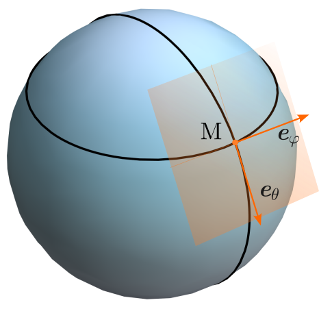
Figure 1: Tangent plane to a sphere and two basis vectors $e_{\varphi}$ and $e_{\theta}$ at a point $\rm M\in S^{2}$.

Next, we recall the expression for an area element on a unit sphere. In standard spherical coordinates $\{\varphi,\theta\}$, it is given by $\Delta A=\sin\theta\Delta\varphi\Delta\theta$ [19]. We interpret this result as an area enclosed by vectors $\Delta\varphi e_{\varphi}$ and $\Delta\theta e_{\theta}$. Now we see that the symplectic form on ${\rm S}^{2}$ is given by [21]

$$\omega=\sin\theta\Big{(}e^{*\varphi}\otimes e^{*\theta}-e^{*\theta}\otimes e^{*\varphi}\Big{)}$$ (57)

so that

$$\omega\Big{(}\Delta\varphi e_{\varphi},\Delta\theta e_{\theta}\Big{)}=\Delta A.$$ (58)

Therefore, the Poisson tensor field is given by

$${\mathcal{P}}=-\left(\sin\theta\right)^{-1}\Big{(}e_{\varphi}\otimes e_{\theta}-e_{\theta}\otimes e_{\varphi}\Big{)}.$$ (59)

Having the Poisson tensor at our disposal, we can calculate Poisson brackets and identify canonical variables. Let us try first with the most obvious choice $X^{1}=\varphi,X^{2}=\theta$. Since $\mathrm{d}\varphi=e^{*\varphi}$ and $\mathrm{d}\theta=e^{*\theta}$, we have

$$\big{[}\varphi,\theta\big{]}_{\rm PB}={\mathcal{P}}\Big{(}\mathrm{d}\varphi,\mathrm{d}\theta\Big{)}=-\frac{1}{\sin\theta}.$$ (60)

Thus, $\varphi$ and $\theta$ are not the canonical variables for ${\rm S}^{2}$. For our second guess, we take $X^{1}=\varphi,X^{2}=\cos\theta$, with $\mathrm{d}\cos\theta=-\sin\theta e^{*\theta}$. Since

$$\big{[}\varphi,\cos\theta\big{]}_{\rm PB}={\mathcal{P}}\Big{(}\mathrm{d}\varphi,\mathrm{d}\theta\Big{)}=1,$$ (61)

we can select $\{\varphi,\cos\theta\}\equiv\{q,p\}$ to be a pair of canonical variables on ${\rm S}^{2}$. This will allow us to define Hamiltonian systems on ${\rm Z}={\rm S}^{2}$ and to study their dynamics. In particular, we shall define classical spins and classical Heisenberg model.

IV.2 A simple quadratic model on ${\rm S}^{2}$

As a warm-up, let us consider a simple quadratic model on the sphere ${\rm S}^{2}$, with Hamiltonian defined as the direct generalization of linear harmonic oscillator

$$H=\frac{p^{2}}{2m}+\frac{m\omega^{2}q^{2}}{2}$$ (62)

with $q=\varphi$ and $p=\cos\theta$. To simplify notation, we choose $m=\omega=1$ so that the quadratic Hamiltonian reduces to

$$H=\frac{\cos^{2}\theta}{2}+\frac{\varphi^{2}}{2}.$$ (63)

Corresponding dual vector field $\mathrm{d}H$ is

$$\mathrm{d}H=-\sin\theta\cos\theta e^{*\theta}+\varphi e^{*\varphi}$$ (64)

and the equations of motion (51) become

$$\frac{\mathrm{d}\varphi}{\mathrm{d}t}=\cos\theta,\hskip 28.45274pt\frac{\mathrm{d}}{\mathrm{d}t}\cos\theta=-\varphi.$$ (65)

To solve this system, we apply the standard procedure and take the second derivative w.r.t time

$$\ddot{\varphi}=\frac{\mathrm{d}}{\mathrm{d}t}\dot{\varphi}={\mathcal{P}}\Big{(}d\dot{\varphi},\mathrm{d}H\Big{)}=-\varphi,$$ (66)

where $\mathrm{d}\dot{\varphi}=\mathrm{d}\cos\theta=-\sin\theta e^{*\theta}$. By choosing $\varphi(0)=\varphi_{0}$ and $\dot{\varphi}(0)=0$, we have

$$\varphi(t)=\varphi_{0}\cos t.$$ (67)

Upon substituting $\varphi(t)$ into the second equation of (65) gives

$$-\dot{\theta}\sin\theta=-\varphi_{0}\cos t,$$ (68)

so that

$$\cos\Big{(}\theta(t)\Big{)}=p(t)=\cos\theta_{0}-\varphi_{0}\sin t,$$ (69)

where $\theta_{0}$ represents the initial value for $\theta(t)$.

Equations (67) and (69) constitute a solution to this simple quadratic model on ${\rm S}^{2}$ and $(\varphi(t),p(t))$ is a parametrized trajectory on two-sphere as a phase space. This solution is presented in FIG. 2, while FIG. 3 shows explicit solutions $\theta(t),\varphi(t)$ and $p(t)=\cos\big{(}\theta(t)\big{)}$. As expected from the Hamiltonian (63), phase-space trajectories resemble those of a simple linear harmonic oscillator. Note that the model (63) does not describe a particle confined to a sphere. For a geometric treatment of classical and quantum particle on a sphere, see [22, 23].

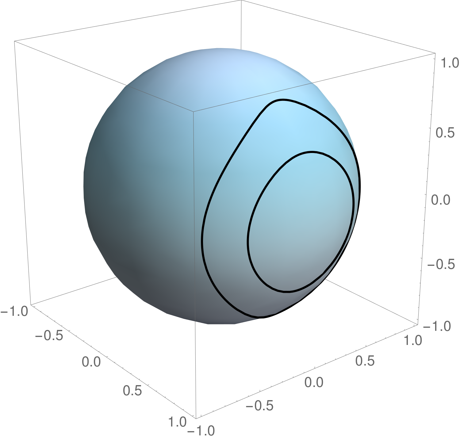
Figure 2: Phase space trajectory $(\varphi(t),p(t)=\cos\theta(t))$ for a simple quadratic Hamiltonian (63) and two sets of initial conditions $(\varphi_{0}=0.5,\cos\theta_{0}=0)$ and $(\varphi_{0}=0.8,\cos\theta_{0}=0)$.

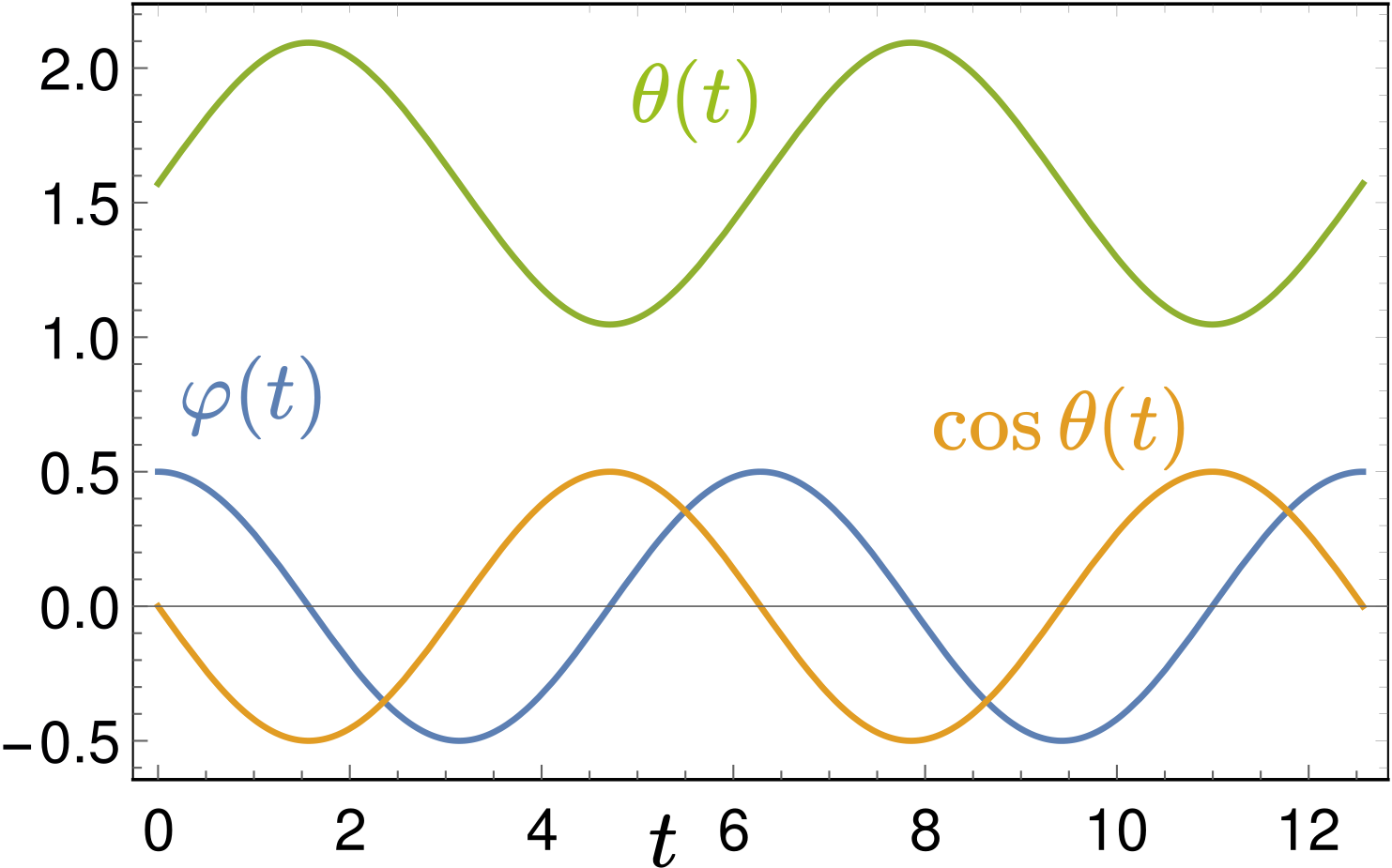
Figure 3: Time evolution of phase space variables $\varphi(t),\theta(t)$ and $p(t)=\cos\theta(t)$ for initial conditions $(\varphi_{0}=0.5,\cos\theta_{0}=0)$.

V Classical Heisenberg model

Now that we have defined the symplectic form and the Poisson tensor, and gained some insight into the phase space ${\rm S}^{2}$ by analyzing a simple harmonic model, we proceed with the study of classical spins.

V.1 Poisson algebra of classical spins

We shall first focus on the case of a single classical spin [24]. A classical unit vector can be represented as

$$\bm{S}=\begin{bmatrix}S_{x}\\ S_{y}\\ S_{z}\\ \end{bmatrix}=\begin{bmatrix}\sin\theta\cos\varphi\\ \sin\theta\sin\varphi\\ \cos\theta\\ \end{bmatrix}$$ (70)

and the condition $|\bm{S}|=1$ follows directly from (70). Since any state of $\bm{S}$ can be uniquely mapped onto a point on a unit sphere, we can consider $\bm{S}$ to be a dynamical variable defined in terms of the canonical pair $\{\varphi,\cos\theta\}$ which parametrizes the phase space ${\rm S}^{2}$. To specify the dynamics, we need a Hamiltonian. However, as we have identified the underlying phase space and corresponding Poisson tensor, we can derive expressions for Poisson brackets of $S_{x},S_{y}$ and $S_{z}$. Note that $S_{x},S_{y}$ and $S_{z}$ are not components of a vector (or a vector field) on ${\rm S}^{2}$. As far as the geometry of phase space is concerned, they are dynamical variables built out of canonical coordinates $\{\varphi,\cos\theta\}$. Because of that, we choose to write $x,y$ and $z$ as lower indices.

Let us calculate first the Poisson bracket of $S_{x}$ and $S_{y}$. According to (52), we have

$$\Big{[}S_{x},S_{y}\Big{]}_{\rm PB}=\mathcal{P}\Big{(}\mathrm{d}S_{x},\mathrm{d}S_{y}\Big{)},$$ (71)

with ${\mathcal{P}}$ given in (59) and

$$\begin{split}\mathrm{d}S_{x}&=-\sin\theta\sin\varphi e^{*\varphi}+\cos\theta\cos\varphi e^{*\theta},\\ \mathrm{d}S_{y}&=\sin\theta\cos\varphi e^{*\varphi}+\cos\theta\sin\varphi e^{*\theta}.\end{split}$$ (72)

Therefore,

$$\begin{split}\Big{[}S_{x},S_{y}\Big{]}_{\rm PB}&=\sin\theta\sin\varphi\frac{\cos\theta}{\sin\theta}\sin\varphi+\cos\theta\cos^{2}\varphi\\ &=\cos\theta=S^{z}.\end{split}$$ (73)

By evaluating the remaining two brackets, and knowing that $\mathcal{P}$ is an antisymmetric tensor, we can show that

$$\Big{[}S_{\alpha},S_{\beta}\Big{]}_{\rm PB}=\varepsilon_{\alpha\beta\gamma}S^{\gamma}$$ (74)

represents the general form of Poisson brackets for classical spins. Here $\varepsilon_{\alpha\beta\gamma}$ represents Levi-Civita symbol [19]. Hence, the algebraic relations under Poisson brackets which components of classical spins satisfy, closely resemble the commutation relations of spin operators (2).

V.2 Hamiltonian and phase space

The classical Heisenberg model is the simplest $\rm O(3)$ invariant model built using the phase space ${\rm S}^{2}$. To construct its Hamiltonian, we need to specify how points on ${\rm S}^{2}$ transform under the action of $\rm O(3)$. The canonical coordinates $\{\varphi,\cos\theta\}$ transform under $\rm O(3)$ according to a nonlinear realization [25] and, because of that, invariant Hamiltonian must include the metric tensor on ${\rm S}^{2}$. On the other hand, the spin vector $\bm{S}$ transforms linearly and the Hamiltonian takes a much simpler form when expressed in terms of $S_{x},S_{y}$ and $S_{z}$.

For simplicity, let us assume a cubic lattice with sites labeled by vector $\bm{n}$ and suppose further that each lattice site hosts a classical spin $\bm{S}_{\bm{n}}$. Since $|\bm{S}_{\bm{n}}|=1$, we can build a Hamiltonian function quadratic in $\bm{S}_{\bm{n}}$ using projections of $\bm{S}_{\bm{n}}$ on $\bm{S}_{\bm{m}}$. If we assume that only nearest-neighbor projections contribute with equal weights $J$, we arrive at the Hamiltonian of classical Heisenberg model

$$H=-\frac{J}{2}\sum_{\bm{n},\bm{\lambda}}\bm{S}_{\bm{n}}\cdot\bm{S}_{\bm{n}+\bm{\lambda}},$$ (75)

where $\{\bm{\lambda}\}$ denotes vectors connecting each site with its nearest neighbors. If $J>0$, the Hamiltonian (75) will give rise to ferromagnetic order [26].

Classical spin configurations satisfy equations of motion which can be obtained using Poisson brackets for classical spins. Since Hamiltonian (75) describes a many-spin system, we need to generalize the Poisson algebra (74). The phase space of classical Heisenberg model is given by Cartesian products of two-spheres for each lattice site

$${\rm{Z}}=\underset{\bm{n}}{\raisebox{-4.5pt}{\scalebox{2.8}{$\times$}}}\left({\rm S}^{2}\right)_{\bm{n}}$$ (76)

and it represents the space of solutions of classical equations of motion [27]. We shall denote spherical coordinates on a unit sphere located at lattice site $\bm{n}$ by $\{\varphi_{\bm{n}},\theta_{\bm{n}}\}$, the tangent vector fields to the unit sphere at $\bm{n}$ by $\{e_{\varphi_{\bm{n}}},e_{\theta_{\bm{n}}}\}$ and the corresponding dual vector fields by $\{e^{*\varphi_{\bm{n}}},e^{*\theta_{\bm{n}}}\}$. The action of dual vector fields on $\{e_{\varphi_{\bm{n}}},e_{\theta_{\bm{n}}}\}$ is given by

$$e^{*\varphi_{\bm{n}}}\Big{(}e_{\varphi_{\bm{m}}}\Big{)}=e^{*\theta{\bm{n}}}\Big{(}e_{\theta{\bm{m}}}\Big{)}=\Delta(\bm{n}-\bm{m}),$$ (77)

where $\Delta(\bm{n}-\bm{m})=1$ only if $\bm{n}=\bm{m}$, $\Delta(\bm{n}-\bm{m})=0$ otherwise, and the symplectic form generalizes to

$$\omega=\sum_{\bm{n}}\sin\theta_{\bm{n}}\Big{(}e^{*\varphi_{\bm{n}}}\otimes e^{*\theta_{\bm{n}}}-e^{*\theta_{\bm{n}}}\otimes e^{*\varphi_{\bm{n}}}\Big{)}.$$ (78)

For each $\bm{n}$, a small variation of a solution of equations of motion can be written as $\delta\bm{S}(\bm{n})=X^{\varphi}\bm{e}_{\varphi_{\bm{n}}}+X^{\bm{\theta}}\bm{e}_{\theta_{\bm{n}}}$ [27] so that $\bm{S}\cdot\delta\bm{S}=0$ and $|\bm{S}+\delta\bm{S}|=1$ within linear approximation in $\delta\bm{S}$. Tensor field $\omega$ measures the area determined by two vector fields in the sense that

$$\omega\Big{(}\Delta\varphi_{\bm{n}}e_{\varphi_{\bm{n}}},\Delta\theta_{\bm{m}}e_{\theta_{\bm{m}}}\Big{)}=\Delta(\bm{n}-\bm{m})\sin\theta_{\bm{m}}\Delta\theta_{\bm{m}}\Delta\varphi_{\bm{n}}.$$ (79)

In complete analogy, we define the Poisson tensor

$${\mathcal{P}}=-\sum_{\bm{n}}\frac{1}{\sin\theta_{\bm{n}}}\Big{(}e_{\varphi_{\bm{n}}}\otimes e_{\theta_{\bm{n}}}-e_{\theta_{\bm{n}}}\otimes e_{\varphi_{\bm{n}}}\Big{)}$$ (80)

so that the Poisson brackets of spin components evaluate to

$$\Big{[}S_{\alpha}(\bm{n}),S_{\beta}(\bm{m})\Big{]}_{\rm PB}=\Delta(\bm{n}-\bm{m})\varepsilon_{\alpha\beta\gamma}S^{\gamma}(\bm{n}),$$ (81)

while fundamental Poisson brackets (61) become

$$\Big{[}\varphi_{\bm{n}},\cos\theta_{\bm{m}}\Big{]}_{\rm PB}=\Delta(\bm{n}-\bm{m}).$$ (82)

Equation (81), together with classical Hamiltonian (75), completely specifies the dynamics of classical spins in Heisenberg model. The Poisson bracket algebra (82) is usually derived starting from commutation relations for spin operators expressed in terms of phase operator $\hat{\varphi}_{\bm{n}}$ and $\hat{S}^{z}_{\bm{n}}$ [28, 29], or postulated [30], while relations (82) are obtained by assuming the correct form of the equations of motion for spins [31]. Here we see that both sets of algebraic relations arise due to symplectic structure on $\rm Z$. The transition to the theory of quantum Heisenberg model can be achieved by standard canonical prescription: replace the classical variable $\bm{S}$ with the operator $\hat{\bm{S}}$ at each lattice site $\bm{n}$ and replace the algebraic structure of Poisson brackets (81) with commutators

$$\Big{[}\;,\;\Big{]}_{\rm PB}\longrightarrow\frac{1}{\mathrm{i}}\Big{[}\;,\;\Big{]}.$$ (83)

This line of reasoning allows us to arrive at the theory of quantum spin systems in a manner which is consistent with standard introduction of operator algebras in quantum systems – by starting from the Poisson algebra of classical dynamical variables and corresponding classical Hamilton function.

V.3 Classical spin waves

To make an analogy with classical field theories of scalar fields, it is useful to rewrite Hamiltonian (75) using the lattice Laplacian. In terms of a site-dependent quantity $\phi$, it is defined as [32]

$$\blacktriangledown^{2}\phi(\bm{x})=\frac{2D}{Z_{1}|\bm{\lambda}|^{2}}\sum_{\{\bm{\lambda}\}}\Big{[}\phi(\bm{x}+\bm{\lambda})-\phi(\bm{x})\Big{]},$$ (84)

where $Z_{1}$ denotes the number of nearest neighbors and $D$ is the dimension of the lattice. In case at hand, $D=3$ and $Z_{1}=6$. A nice property of the lattice Laplacian is that its eigenfunctions are plane waves

$$\blacktriangledown^{2}\exp[\mathrm{i}\bm{k}\cdot\bm{x}] =-\frac{2D}{|\bm{\lambda}|^{2}}[1-\gamma_{D}(\bm{k})]\exp[\mathrm{i}\bm{k}\cdot\bm{x}]$$

$$\equiv-\mathcal{K}^{2}\exp[\mathrm{i}\bm{k}\cdot\bm{x}],$$ (85)

where

$$\gamma_{D}(\bm{k})=Z_{1}^{-1}\sum_{\{\bm{\lambda}\}}\exp[\mathrm{i}\bm{k}\cdot\bm{\lambda}].$$ (86)

The lattice Laplacian is designed in such a way that

$$\lim_{|\bm{\lambda}|\to 0}\mathcal{K}^{2}=\bm{k}^{2}+\mathcal{O}(k^{4})$$ (87)

and, consequently,

$$\blacktriangledown^{2}\phi(\bm{x})=\nabla^{2}\phi(\bm{x})+\mathcal{O}(|\bm{\lambda}|^{2})$$ (88)

with $\nabla^{2}$ denoting standard Laplacian operator. Hamiltonian (75) can be rewritten using lattice Laplacian as

$$H=-\frac{1}{2}\;\frac{JZ_{1}|\bm{\lambda}|^{2}}{2D}\sum_{\bm{n}}\bm{S}_{\bm{n}}\cdot\blacktriangledown^{2}\bm{S}_{\bm{n}}-\frac{JZ_{1}N}{2},$$ (89)

where $N$ denotes the number of sites in the lattice.

Equations of motion are now given by (51), with $f$ denoting components of $\bm{S}_{\bm{n}}$, $H$ given in (89) and $\mathcal{P}$ defined in (80). Thus,

$$\dot{\bm{S}}(\bm{n},t) =\Big{[}\bm{S}(\bm{n},t),H\Big{]}_{\rm PB}=\Big{[}S_{\beta}(\bm{n},t),H\Big{]}_{\rm PB}\bm{e}_{\beta}$$

$$=\frac{JZ_{1}|\bm{\lambda}|^{2}}{2D}\varepsilon_{\gamma\alpha\beta}S_{\gamma}(\bm{n},t)\blacktriangledown^{2}S_{\alpha}(\bm{n},t)\bm{e}_{\beta},$$

$$=\frac{JZ_{1}|\bm{\lambda}|^{2}}{2D}\bm{S}(\bm{n},t)\times\blacktriangledown^{2}\bm{S}(\bm{n},t),$$ (90)

where we have used (81) and (53). The equation (90) is a discretized version of the Landau-Lifshitz equation.

At this point we are going to make an approximation by assuming that spin configurations governed by (90) describe small deviations from a uniform $[0,0,1]^{\rm T}=\bm{e}_{z}$ state. Therefore, we take $\bm{S}$ to be of the form $[\delta S_{x},\delta S_{y},1]^{\rm T}$, with $(\delta S_{x})^{2},(\delta S_{y})^{2}\ll 1$ and $\dot{S}_{z}=0$. The equation (90) now reduces to

$$\dot{\delta S_{x}}(\bm{n},t) =-\frac{JZ_{1}|\bm{\lambda}|^{2}}{2D}\blacktriangledown^{2}S_{y}(\bm{n},t),$$

$$\dot{\delta S_{y}}(\bm{n},t) =\frac{JZ_{1}|\bm{\lambda}|^{2}}{2D}\blacktriangledown^{2}S_{x}(\bm{n},t).$$ (91)

As we shall see now, these two equations describe a single physical degree of freedom. This is most easily seen by defining a complex field

$$\psi(\bm{n},t):=\frac{\delta S_{x}(\bm{n},t)+\mathrm{i}\delta S_{y}(\bm{n},t)}{\sqrt{2}}$$ (92)

so that the equation of motion for $\psi$ takes the form of a Schrödinger equation

$$\mathrm{i}\dot{\psi}(\bm{n},t)=-\frac{1}{2m}\blacktriangledown^{2}\psi(\bm{n},t),$$ (93)

where

$$m:=\frac{D}{JZ_{1}|\bm{\lambda}|^{2}}$$ (94)

is a parameter that depends on the strength of the coupling $J$ and the structure of the lattice. The field $\psi$, which describes small fluctuations around the ferromagnetic ground state, is the classical spin wave. Being linear, equation (93) can be solved by Fourier transform

$$\hskip-11.38092pt\psi(\bm{n},t)=\int_{\bm{k}}a_{\bm{k}}\;\mathrm{e}^{\mathrm{i}\bm{k}\cdot\bm{x}-\omega(\bm{k})t},\hskip 14.22636pt\int_{\bm{k}}\equiv\int_{\rm{IBZ}}\frac{\mathrm{d}^{D}\bm{k}}{(2\pi)^{D}}$$ (95)

where

$$\omega(\bm{k})=\frac{\widehat{\bm{k}}^{2}}{2m}$$ (96)

and $a_{\bm{k}}$ are complex amplitudes and $\int_{\rm{IBZ}}$ denotes integration over the first Brillouin zone.

It is easy to see that the equation of motion (93) follows from the Hamiltonian

$$H_{\rm{LSW}}=-\frac{1}{2m}\sum_{\bm{n}}\psi^{*}(\bm{n},t)\blacktriangledown^{2}\psi(\bm{n},t)$$ (97)

and Poisson brackets

$$\Big{[}\psi(\bm{n},t),\psi^{*}(\bm{m},t)\Big{]}_{\rm{PB}}=-\mathrm{i}\Delta(\bm{n}-\bm{m}),$$ (98)

where

$$\Big{[}F,G\Big{]}_{\rm{PB}}=\sum_{\bm{n}}\left(\frac{\partial F}{\partial\psi(\bm{n})}\frac{\partial G}{\partial\psi^{*}(\bm{n})}-\frac{\partial F}{\partial\psi^{*}(\bm{n})}\frac{\partial G}{\partial\psi(\bm{n})}\right).$$ (99)

This motivates us to define conjugate momentum $\pi:=\mathrm{i}\psi^{*}$, so that

$$\Big{[}\psi(\bm{n},t),\pi(\bm{m},t)\Big{]}_{\rm{PB}}=\Delta(\bm{n}-\bm{m}).$$ (100)

Indeed, these all are well-known results in the theory of classical Schrödinger field [2]. The symplectic form of the linearized system is given by

$$\omega=\sum_{\bm{n}}\Big{(}e^{*\psi_{\bm{n}}}\otimes e^{*\pi_{\bm{n}}}-e^{*\pi_{\bm{n}}}\otimes e^{*\psi_{\bm{n}}}\Big{)}$$ (101)

and it describes a symplectic structure on the phase space $\mathbb{R}^{2N}$, which is the space of plane-wave solutions. In the context of classical spin waves, the linearization process may be viewed as the transition from (78) to (101).

To summarize, classical field configurations which describe small deviations from the ferromagnetic ground state $\bm{S}(\bm{n},t)=\bm{e}_{z}$ are given by (superposition of) plane waves with dispersion relation (96). In modern nomenclature, they are classified as Nambu-Goldstone fields of type B [33, 34]. Upon quantization, these will become elementary excitations – magnons.

We see from (87) and (96) that in the low-energy limit $\omega(\bm{k})\approx\bm{k}^{2}/(2m)$, so that ferromagnetic magnons behave like nonrelativistic particles. This is not a universal feature of Nambu-Goldstone bosons as evidenced from the cases of antiferromagnetic magnons, phonos or pions which all exhibit relativistic dispersion relation $\omega(\bm{k})\propto|\bm{k}|$ [30]. It turns out that nonrelativistic dispersion relation is a consequence of symplectic form defined on configuration space of the magnon fields, which is also ${\rm S^{2}}$. This symplectic form, also known as Kirillov-Kostant symplectic form, is induced by spontaneous magnetization and it is responsible for pairing two components $\{S_{x}(\bm{x},t)$, $S_{y}(\bm{x},t)\}$ into a single physical degree of freedom $\psi(\bm{x},t)$ [34].

VI Alternative definition of Poisson brackets

As we have seen, the Poisson tensor can be used to define Poisson brackets on a non-Euclidean phase space. However, there is an equivalent definition in terms of the symplectic form. Since the symplectic form is a $(0,2)$ type tensor field, it naturally acts on pair of vector fields and these vector fields must be associated to the pair of functions $f,g$ whose brackets we wish to define.

We shall denote the vector field corresponding to the function $f$ by $X_{f}$ and define it in terms of $\mathrm{d}f$ [14]

$$X_{f}={\mathcal{P}}\Big{(}\rule{11.38092pt}{0.42677pt},\mathrm{d}f\Big{)}.$$ (102)

This definition resembles the usual index gymnastics described in Section II.3 except the fact that ${\mathcal{P}}$ is an antisymmetric rather than a symmetric tensor field. The Poisson bracket is now given by [21]

$$\Big{[}f,g\Big{]}_{\rm{PB}}:=\omega\Big{(}X_{f},X_{g}\Big{)},$$ (103)

where $f$ and $g$ are functions on $\rm Z$.

Of course, we need to show that (103) coincides with (52). First of all, we see from (102) that the components of the associated vector field $X_{f}$ are given by $(X_{f})^{i}={\mathcal{P}}^{ik}\partial_{k}f$. Now

$$\omega\Big{(}X_{f},X_{g}\Big{)} =\omega_{ij}(X_{f})^{i}(X_{g})^{j}=\omega_{ij}{\mathcal{P}}^{ik}{\mathcal{P}}^{jl}\partial_{k}f\partial_{l}g$$

$$=-\omega_{ji}{\mathcal{P}}^{ik}{\mathcal{P}}^{jl}\partial_{k}f\partial_{l}g$$

$$={\mathcal{P}}\Big{(}\mathrm{d}f,\mathrm{d}g\Big{)}=\Big{[}f,g\Big{]}_{\rm{PB}},$$ (104)

where we have used (50). The two definitions are, therefore, completely equivalent and all results regarding the phase space $\rm S^{2}$ and classical Heisenberg model could be derived starting from (103).

VII Symplectic manifolds

The purpose of this section is to provide some details on manifolds, and symplectic manifolds in particular. The exposition is elementary and a complete treatment can be found in [14, 35, 36].

First of all, a manifold is defined to be a space which locally looks like $\mathbb{R}^{n}$. For example, a sphere looks locally like $\mathbb{R}^{2}$ since the vicinity of each point on the sphere can be mapped on a two dimensional Euclidean space by a one-to-one continuous map [14, 15]. The equivalence between $\rm S^{2}$ and $\mathbb{R}^{2}$ does not hold globally, however. Symplectic manifolds carry additional structure – a closed non-degenerate antisymmetric tensor field of type $(0,2)$. The condition of the symplectic form being closed amounts to Poisson brackets satisfying the Jacobi identity. Non-degeneracy of an antisymmetric tensor field means that we require non-degeneracy of symplectic form at each point on the manifold. Given a point $\rm M$ of the manifold and a tangent vector to the manifold at the same point $\rm M$, $X_{\rm M}$, the symplectic form at this point, $\omega_{\rm M}$, is non-degenerate if $\omega_{\rm M}(X_{\rm M},Y_{\rm M})=0$ implies $Y_{\rm M}=0$. The condition of non-degeneracy seems to be in conflict with our definition of symplectic form on $\rm S^{2}$ given in (57).

To see that the symplectic form (57) is truly non-degenerate, we shall first show that it can be defined in a coordinate-free manner. For a point $\rm{M}\in{\rm S}^{2}$, determined by the unit vector $\bm{e}_{r}$, and two tangent vectors $X_{\rm M},Y_{\rm M}$ at the same point, the symplectic form is defined by

$$\omega_{\rm M}(X_{\rm M},Y_{\rm M}):=-\bm{e}_{r}\cdot(\bm{X}\times\bm{Y}),$$ (105)

where $\bm{X},\bm{Y}\in\mathbb{R}^{3}$ are vectors tangent to the sphere at $\rm M$ (corresponding to $X_{\rm M}$ and $Y_{\rm M}$, respectively), $\times$ denotes cross product of vectors in $\mathbb{R}^{3}$, $\cdot$ is the standard inner product on $\mathbb{R}^{3}$ and the negative sign is just for convention. The form $\omega$ is obviously well defined at all points $\rm{M}\in{\rm S}^{2}$. The non-degeneracy condition for $\omega_{\rm M}$ is now easily established since, given two nonzero and non-collinear vectors $X_{\rm M},Y_{\rm M}$ at the same point, $\bm{X}\times\bm{Y}$ is parallel to $\bm{e}_{r}$ and, consequently $\omega_{\rm M}(X_{\rm M},Y_{\rm M})\neq 0$. To show that (105) is equivalent to (57), we simply evaluate components of $\omega$ at point $\rm M$ determined by $\bm{e}_{r}=\sin\theta(\bm{e}_{x}\cos\varphi+\bm{e}_{y}\sin\varphi)+\bm{e}_{z}\cos\theta$. By remembering that $e_{\varphi}$ corresponds to $\sin\theta\bm{e}_{\varphi}$, and that $\bm{e}_{\theta}\times\bm{e}_{\varphi}=\bm{e}_{r}$, we get

$$\omega_{\varphi\theta}\left.\right|_{\rm M} =\omega(e_{\varphi},e_{\theta})\left.\right|_{\rm M}=-\bm{e}_{r}\cdot\Big{(}\sin\theta\bm{e}_{\varphi}\times\bm{e}_{\theta}\Big{)}$$

$$=\sin\theta$$ (106)

in complete agreement with (57). Thus, the symplectic form $\omega$ is indeed defined at all points of a sphere and the apparent vanishing of $\omega$ at poles is just an artifact of standard spherical coordinates. These problems can be evaded if several coordinate systems are used to cover $\rm S^{2}$.

Finally, we give a few remarks on notation. A coordinate basis of vector fields, on a patch of a manifold covered by local coordinates $\{x^{\mu}\}$, is commonly denoted by $\{\partial/\partial x^{\mu}\equiv\partial_{\mu}\}$. The corresponding basis of dual vector fields is denoted by $\{\mathrm{d}x^{\mu}\}$, so that $\mathrm{d}x^{\mu}(\partial_{\nu})=\delta^{\mu}_{\nu}$. Using this notation, (45) becomes simply $\mathrm{d}H=\partial_{1}H\mathrm{d}x^{1}+\partial_{2}H\mathrm{d}x^{2}$. Also, when working with antisymmetric tensors, one is naturally led to the concept of exterior (or wedge) product – antisymmetric tensor product defined as $\mathrm{d}x^{\mu}\wedge\mathrm{d}x^{\nu}:=\mathrm{d}x^{\mu}\otimes\mathrm{d}x^{\nu}-\mathrm{d}x^{\nu}\otimes\mathrm{d}x^{\mu}$. Using the wedge product, the symplectic form (57) can be written as

$$\omega=\sin\theta\mathrm{d}\varphi\wedge\mathrm{d}\theta.$$ (107)

One can easily rewrite all the other tensor fields used in this article in a similar fashion (See [15, 14]).

VIII Summary

Quantum Heisenberg model describes the physics of localized magnetism. As such, it has many important applications in modeling strongly correlated electron systems. It exhibits spontaneous symmetry breaking, emergent degrees of freedom carried by quasi-particles, as well as a rich phase diagram controlled by various coupling constants, anisotropy parameters, etc., which makes it important from a pedagogical point of view also. However, it is rarely discussed in the context of quantization since Poisson brackets for classical spins are not of a simple form usually taught to undergraduate physics students. Because of that, Heisenberg model is commonly introduced directly as a quantum model and classical Heisenberg ferromagnet does not get a portion of the attention it deserves.

The reason for avoiding detailed discussion on classical Heisenberg model in introductory statistical mechanics courses lies in the simple fact: The phase space for a single classical spin is not a Euclidean space and the standard definition of Poisson brackets does not apply in this case. We provide here step-by-step derivation of the Poison bracket algebra of classical spins based on the symplectic form on two-sphere. The presentation is elementary: we assume only knowledge of basic tensor algebra and curvilinear spherical coordinates. Besides allowing for a discussion on classical spin waves as collective degrees of freedom which eventually become magnons, arguments presented here put classical Heisenberg model into a broader context of quantization of systems defined on non-Euclidean phase spaces and limitations of standard canonical prescription.

Many excellent books emphasizing the importance of symplectic and Poisson structures in contemporary physics do exist. Besides already mentioned [14, 15], an interested reader could also consult classic texts [36, 35, 21] or a recent review [37]. Also, Landau-Lifshitz equation and its solutions are discussed in [38, 39], while some references on Monte Carlo simulations of classical Heisenberg model are [40, 41, 42, 43]. The physics of Nambu-Goldstone bosons is covered in [30] as well as in [44, 45].