Persistent Stiefel–Whitney Classes of Tangent Bundles

Abstract

Stiefel–Whitney classes are invariants of the tangent bundle of a smooth manifold, represented as cohomology classes of the base manifold. Given a point cloud, we construct a Čech or alpha filtration. By applying the Wu formula in a persistent setting, we derive a sequence of persistent cohomology classes from the filtration. We show that if the filtration is homotopy equivalent to a smooth manifold, then one of these persistent cohomology classes corresponds to the $k$-th Stiefel–Whitney class of the tangent bundle of that manifold. To demonstrate the effectiveness of our approach, we present experiments on real-world datasets.

1 Introduction

The tangent bundle of a smooth manifold consists of its all tangent spaces and plays a fundamental role in differential geometry and topology ([1, 2]). The Stiefel–Whitney classes of the tangent bundle are characteristic cohomology classes that serve as powerful invariants of the base manifold ([3, 4, 5]). For example, a smooth manifold is orientable if and only if the first Stiefel–Whitney class of its tangent bundle vanishes. More generally, higher Stiefel–Whitney classes impose additional obstructions, such as constraints on whether a smooth manifold can be embedded into Euclidean space of a given dimension.

Here is an intuitive example illustrating the significance of the Stiefel–Whitney classes. The torus and the Klein bottle cannot be differentiated by their cohomology with coefficients in $\mathbb{Z}/2$, but the first Stiefel–Whitney class of their tangent bundles distinguishes them. More broadly, every closed surface can be completely classified by its Euler characteristic and the first Stiefel–Whitney class of its tangent bundle.

Topological Data Analysis (TDA) applies algebraic topology to extract topological features from point clouds embedded in high-dimensional spaces ([6, 7, 8]). A central tool, persistent (co)homology, tracks connected components, loops, and higher-dimensional cycles across multiple scales in a filtration. Although recent work has introduced methods for computing Stiefel–Whitney classes in a persistent setting ([9, 10, 11]), many aspects remain unexplored. A fundamental challenge in computing characteristic classes in the persistent setting is that vector bundles are traditionally defined over a single CW complex, whereas persistent topology operates on filtrations of simplicial complexes. Recent studies have made progress in bridging this gap.

Tinarrage ([9]) proposed a method for defining and computing persistent Stiefel–Whitney classes using a vector bundle filtration. It utilized the simplicial classifying map of the topological space into an infinite projective space, restricting it to rank-1 (line) bundles and preventing extension to tangent bundles. The issue arises because while the projective space $\mathbb{RP}^{m}$ large $m$ approximates the classifying space for line bundles, the corresponding space for higher-rank vector bundles is the $n$-dimensional Grassmannian $\mathbf{Gr}_{n}(\mathbb{R}^{m})$, which has a highly complex triangulation when $n\geq 2$.

In an alternative approach, Scoccola and Perea ([10]) computed the first and second characteristic classes using a discrete approximate $O(d)$-valued 1-dimensional cocycle, derived by estimating the tangent spaces via local PCA ([12]). Their framework is well-suited for discrete data, but its reliance on geometric estimates limits its natural extension to persistent cohomology.

Ren ([11]) defined a persistent vector bundle as a sequence of functorial pullback bundles and independently introduced persistent Stiefel–Whitney classes, distinct from those in [9]. In that work, these classes were used to provide obstructions to embedding problems in configuration spaces of hard spheres.

Wu ([13]) introduced the Wu formula for determining Stiefel–Whitney classes of tangent bundles using the cup product and Steenrod squares. A primary advantage is that it extracts Stiefel–Whitney classes of the tangent bundle directly from the cohomology ring of the base manifold. Moreover, since the cup product and Steenrod squares are functorial, they naturally extend to operations on cohomology barcodes ([14]). Consequently, Wu’s approach may allow the definition and computation of persistent Stiefel–Whitney classes based on persistent cohomology operations.

In this work, we establish a novel methodology for computing persistent cohomology classes that correspond to the Stiefel–Whitney classes of the tangent bundle of the smooth manifold in a persistent manner. First, we introduce the definitions of persistent vector bundle and vector bundle filtration in [11] and [9], establish their equivalence, and prove that they yield the same persistent Stiefel–Whitney classes. We define the persistent Wu classes and persistent Stiefel–Whitney classes of type $n$, characterized by the Wu criterion in persistent topology. Our main theorem demonstrates that if a filtration is homotopy equivalent to an $n$-dimensional smooth manifold, then the persistent Stiefel–Whitney classes of type $n$ of the filtration always exist and represent the Stiefel–Whitney classes of the tangent bundle of the manifold.

Theorem 1.1 (Theorem 3.1).

Let $\mathbb{X}=\{X^{r}\}_{r\in[s,t]}$ be a filtration of spaces defined on a filtration interval $[s,t]$. Suppose that for every $s\leq r\leq t$, each space $X^{r}$ deformation retracts onto a smooth $n$-dimensional manifold $M$. Then, for $1\leq k\leq n$, the $k$-th persistent Stiefel–Whitney class $\mathbb{w}_{k}$ of the vector bundle filtration associated with the classifying map of the tangent bundle of $M$ and the family of homotopy equivalences, exists and can be computed using the persistent Wu formula (Definition 3.7).

We propose an algorithm to compute persistent Stiefel–Whitney classes of type $n$, based on Theorem 3.1. The pipeline consists of the following steps:

1. Construct a filtration of simplicial complexes $\mathbb{X}=\{X^{r}\}_{r\in[s,t]}$ over the filtration interval $[s,t]$ from the sampled data $P=\{p_{i}\}_{i=1}^{N}\subset\mathbb{R}^{D}$, using either the Čech or the Alpha filtration.

2. Compute the persistent cohomology $H^{*}(\mathbb{X};\mathbb{Z}/2)$ over $[s,t]$ and extract representative cocycles at the filtration scale $t$.

3. Compute $\{v_{(k,n)}^{t}\}_{k=0}^{n}$, the Wu classes of type $n$ at scale $t$, ensuring that they satisfy the Wu criterion (cf. Remark 2.1):

   $$v_{(k,n)}^{t}\smile x=\operatorname{Sq}^{k}(x)\quad\text{for every }x\text{ in a basis of }\in H^{n-k}(X^{t};\mathbb{Z}/2).$$

   Here, the computations of the cup product and Steenrod squares follow from Algorithm 3 and Algorithm 5, respectively.

4. Compute the $k$-th Stiefel–Whitney class of type $n$ at scale $t$, denoted by $w_{(k,n)}^{t}$, using the Wu formula:

   $$w_{(k,n)}^{t}=\sum_{i+j=k}\operatorname{Sq}^{i}(v_{(j,n)}^{t}).$$

5. Check that for every persistent cohomology $\mathbb{x}_{l}=\{x_{l}^{r}\}_{r\in[s_{l},t_{l}]}\in H^{n-k}(\mathbb{X};\mathbb{Z}/2)$ with its barcode $[s_{l},t_{l}]$ satisfying $s\leq t_{l}<t$, the Wu criterion holds at each right endpoint $t_{l}$ (cf. Remark 3.1):

   $$v_{(k,n)}^{t_{l}}\smile x_{l}^{t_{l}}=\operatorname{Sq}^{k}(x_{l}^{t_{l}}),\quad v_{(k,n)}^{t_{l}}=\iota_{t_{l}}^{t*}v_{(k,n)}^{t}.$$

6. If this condition holds for all relevant cases, compute the $k$-th persistent Stiefel–Whitney class of type $n$ using the persistent Wu formula (cf. Definition 3.7):

   $$\mathbb{w}_{(k,n)}=\sum_{i+j=k}\operatorname{Sq}^{i}(\mathbb{v}_{(j,n)})=\left\{\iota_{r}^{t*}\left[\sum_{i+j=k}\operatorname{Sq}^{i}(v_{(j,n)}^{t})\right]\right\}_{r\in[s,t]}.$$

To illustrate the applicability of our theory to real-world data, we present the results of three numerical experiments. All Python implementation codes are available at https://github.com/Dongwoo-Gang/sw-using-wu/tree/master.

Outline of the Paper

The paper begins in Section 2 with a brief introduction to vector bundle theory and persistence theory. In Section 3, we introduce persistent Stiefel–Whitney classes in two ways, prove their equivalence, and develop an algorithm to compute them using the Wu formula. In Section 4, we prove the existence persistent Stiefel–Whitney classes with high probability. Section 5 presents a pipeline for finding persistent Stiefel–Whitney classes. In Section 6, we present results from numerical experiments on structured datasets, including applications to complex manifolds, image patches, and molecular conformation space.

2 Theoretical background

2.1 Cohomology operations

In this subsection, we present the combinatorial definitions of two cohomology operations, the cup product and Steenrod squares, following [14]. For their construction and topological significance, see [15], Chapters 3–4.

Let $X$ be a simplicial complex. For a ring $R$, let $H^{p}(X;R)$ denote the $p$-th singular cohomology of $X$ with coefficients in $R$. Given two cohomology classes $\alpha\in H^{p}(X;R)$ and $\beta\in H^{q}(X;R)$, their cup product $\alpha\smile\beta\in H^{p+q}(X;R)$ is defined by

$$(\alpha\smile\beta)(\sigma)=(-1)^{p+q}\alpha([v_{0},\ldots,v_{p}])\cdot\beta([v_{p},\ldots,v_{p+q}]).$$

for a given $(p+q)$-dimensional simplex $\sigma=[v_{0},\ldots,v_{p+q}]$ of $X$. This operation is bilinear, associative, and satisfies the graded-commutativity $\alpha\smile\beta=(-1)^{pq}\beta\smile\alpha$. Moreover, the cup product is functorial with respect to pullbacks, that is, if $f:X\to Y$ is a continuous map between topological spaces, then for all $\alpha\in H^{p}(Y;R)$ and $\beta\in H^{q}(Y;R)$, we have $f^{*}(\alpha\smile\beta)=f^{*}\alpha\smile f^{*}\beta.$ The cup product endows $H^{*}(X;R)$ with a graded-commutative algebra structure.

Steenrod squares are a unique family of cohomology operations $\operatorname{Sq}^{i}:H^{p}(X;\mathbb{Z}/2)\to H^{p+i}(X;\mathbb{Z}/2)$ satisfying the following properties.

• Naturality : For a map $f:X\to Y$ and $\alpha\in H^{*}(Y;\mathbb{Z}/2)$, $f^{*}\operatorname{Sq}^{k}(\alpha)=\operatorname{Sq}^{k}(f^{*}\alpha)$.

• $\operatorname{Sq}^{0}=id$.

• If $|x|=i$, then $\operatorname{Sq}^{i}(x)=x^{2}=x\smile x$.

• If $|x|<i$, then $\operatorname{Sq}^{i}(x)=0$.

• Cartan formula : $\operatorname{Sq}^{k}(x\smile y)=\sum_{i+j=k}\operatorname{Sq}^{i}(x)\smile\operatorname{Sq}^{j}(y)$ .

In this work, we adopt an approach for computing Steenrod Squares based on cup-$i$ coproduct, as described in [16], and implement it in Algorithms 4 and 5 .

Definition 2.1 ([16], Cup-$i$ Coproduct).

For a simplicial complex $X$ and $i\in\mathbb{N}\cup\{0\}$, let $\sigma=[0,1,\ldots,p]\in X$. Define the cup-$i$ coproduct as

$$\Delta_{i}:H_{p}(X;\mathbb{Z}/2)\rightarrow H_{p+i}(X;\mathbb{Z}/2),$$

$$\Delta_{i}(\sigma)=\sum_{U\subset\{0,1,\ldots,p\},\,|U|=p-i}d_{U^{0}}(\sigma)\otimes d_{U^{1}}(\sigma)\in(C_{*}(X;\mathbb{Z}/2)\otimes C_{*}(X;\mathbb{Z}/2))_{p+i},$$

where the sum is taken over all subsets $U=\{u_{1},\ldots,u_{p-i}\}$ of $\{0,1,\ldots,p\}$ with $|U|=p-i$. Here, the subsets $U^{0}$ and $U^{1}$ are defined as $U^{0}=\{u_{j}\in U\mid j\text{ is even}\}$ and $U^{1}=\{u_{j}\in U\mid j\text{ is odd}\}$, respectively. For $V=\{v_{1},\ldots,v_{k}\}\subset\{0,1,\ldots,p\}$, $d_{V}(\sigma)$ is defined as $d_{V}(\sigma)=[0,\ldots,\hat{v_{1}},\ldots,\hat{v_{k}},\ldots,p]$.

Theorem 2.1 ([16]).

For $[\alpha]\in H^{p}(X;\mathbb{Z}/2)$ and $k\in\mathbb{N}\cup\{0\}$ with $k\leq p$, we have

$$\operatorname{Sq}^{k}([\alpha])=[(\alpha\otimes\alpha)\Delta_{p-k}(\cdot)]\in H^{p+k}(X;\mathbb{Z}/2).$$

2.2 Vector bundle and Stiefel–Whitney class

In this subsection, we refer to [3], Sections 4–8. A vector bundle $\xi=(E,B)$ of rank $n$ consists of a topological space $E$ called the total space, a base space $B$, and a continuous projection $\pi:E\to B$, such that each fiber $\pi^{-1}(b)$ is an $n$-dimensional vector space. Locally, for each $b\in B$, there exists an open neighborhood $U\subset B$ of $b$ and a homeomorphism $\phi:\pi^{-1}(U)\to U\times\mathbb{R}^{n}$ such that the restriction of $\pi$ to $\pi^{-1}(U)$ corresponds to the projection onto $U$. A vector bundle is called a trivial bundle or product bundle if there exists a global homeomorphism $E\cong B\times\mathbb{R}^{n}$ that respects the projection $\pi$.

A bundle map between two vector bundles $\xi_{1}=(E_{1},B_{1})$ and $\xi_{2}=(E_{2},B_{2})$ is a continuous map $G:E_{1}\to E_{2}$ that maps each fiber $\pi^{-1}(b)$ of $\xi_{1}$ to the corresponding fiber $\pi^{-1}(b^{\prime})$ of $\xi_{2}$ via a linear isomorphism. The induced map $\hat{G}:B_{1}\to B_{2}$ describes how base points are mapped. Two vector bundles $\xi_{1}$ and $\xi_{2}$ are isomorphic if there exists a homeomorphism $G:E_{1}\to E_{2}$ that is a bundle map. If $\xi_{1}$ and $\xi_{2}$ share the same base space $B$, a bundle map over $B$ is a bundle map $G:E_{1}\to E_{2}$ such that the induced map $\hat{G}:B\to B$ is the identity map.

Given two maps $f:X\to B$ and $g:Y\to B$, their fiber product is the space

$$X\times_{B}Y=\{(x,y)\in X\times Y\mid f(x)=g(y)\},$$

equipped with the projection maps $p_{X}:X\times_{B}Y\to X$ and $p_{Y}:X\times_{B}Y\to Y$, satisfying the commutative diagram

$$\leavevmode\hbox to80.93pt{\vbox to48.32pt{\text{[drawing]}}}. {X\times_{B}Y} {Y} {X} {B} \scriptstyle{p_{X}} \scriptstyle{p_{Y}} \scriptstyle{g} \scriptstyle{f}$$

Given a vector bundle $\xi=(E,B)$ and a map $f:X\to B$, we define the pullback bundle $f^{*}\xi=(f^{*}E,X)$ as a vector bundle over $X$ whose fibers correspond to those of $\xi$ at the image points of $f$. The total space of $f^{*}\xi$ is defined as the fiber product $f^{*}E=E\times_{B}X$ of two maps $f:X\to B$ and $\pi:E\to B$. The projection $f^{*}E\to X$ is given by $(e,x)\mapsto x$, and the fiber over each $x\in X$ is naturally isomorphic to the fiber $\pi^{-1}(f(x))$ of $E$ at $f(x)$.

For two vector bundles $\xi_{1}=(E_{1},B_{1})$ and $\xi_{2}=(E_{2},B_{2})$ with projections $\pi_{1}$ and $\pi_{2}$, define the Cartesian product $\xi_{1}\times\xi_{2}=(E_{1}\times E_{2},B_{1}\times B_{2})$ as the bundle with projection map $\pi=(\pi_{1},\pi_{2}):E_{1}\times E_{2}\to B_{1}\times B_{2}.$ Let $\xi_{1}=(E_{1},B)$ and $\xi_{2}=(E_{2},B)$ be two vector bundles over a common base space $B$ and let $d:B\to B\times B$ be the diagonal map. The bundle $d^{*}(\xi_{1}\times\xi_{2})$ over $B$ is called the Whitney sum of $\xi_{1}$ and $\xi_{2}$, denoted by $\xi_{1}\oplus\xi_{2}$.

The Möbius bundle $\gamma_{1}^{1}=(M,S^{1})$ is defined as

$$M=\{(x,y)\in[0,1]\times\mathbb{R}\mid(0,y)\sim(1,-y)\},\quad S^{1}=[0,1]/\{0\sim 1\},$$

where the projection map is defined as the projection onto the first coordinate. This is the nontrivial line bundle over the circle.

A key tool for studying vector bundles is the concept of characteristic classes, which capture topological obstructions to a bundle being trivial. These classes provide cohomological invariants that measure how a vector bundle differs from a trivial bundle([5], Part 3). An important characteristic class is the Stiefel–Whitney class. For a vector bundle $\xi=(E,B)$ of finite rank, we define the Stiefel–Whitney classes $\{w_{k}(\xi)\}_{k\in\mathbb{N}\cup\{0\}}$ of $\xi$ as the cohomology classes of $B$ with coefficients in $\mathbb{Z}/2$ that satisfy the following axioms:

• For every vector bundle $\xi$, $w_{0}(\xi)=1\in H^{0}(B,\mathbb{Z}/2)$ is the unit element in the cohomology ring $H^{*}(B;\mathbb{Z}/2)$, and $w_{k}(\xi)=0$ if $\text{rank }(\xi)<k.$

• For vector bundles $\xi_{1}=(E_{1},B_{1})$, $\xi_{2}=(E_{2},B_{2})$ and a bundle map $f:E_{1}\to E_{2}$, we have $f^{*}w_{i}(\xi_{2})=w_{i}(\xi_{1}).$

• If we write $w(\xi)=\sum_{i=0}w_{i}(\xi)\in H^{*}(B;\mathbb{Z}/2)$, then for another bundle $\eta$ whose base is $B$, $w(\xi\oplus\eta)=w(\xi)\smile w(\eta).$

• $w_{1}(\gamma_{1}^{1})\neq 0$, where $\gamma_{1}^{1}$ is the Möbius bundle over $S^{1}.$

We call $w_{k}(\xi)\in H^{k}(B;\mathbb{Z}/2)$ the $k$-th Stiefel–Whitney class of the vector bundle $\xi$. For a smooth manifold $M$, the $k$-th Stiefel–Whitney class of $M$ refers to the $k$-th Stiefel–Whitney class of its tangent bundle $TM$, denoted $w_{k}(M)$.

Another perspective on Stiefel–Whitney classes arises from the theory of classifying spaces for vector bundles. The space $\mathbb{R}^{\infty}$ is defined as the direct limit of the sequence

$$\mathbb{R}^{1}\subset\mathbb{R}^{2}\subset\mathbb{R}^{3}\subset\cdots,$$

endowed with the direct limit topology. The $n$-dimensional real infinite Grassmannian $\mathbf{Gr}_{n}(\mathbb{R}^{\infty})$ is the topological space of all $n$-dimensional linear subspaces of $\mathbb{R}^{\infty}$, defined as

$$\mathbf{Gr}_{n}(\mathbb{R}^{\infty}):=\{V\subset\mathbb{R}^{\infty}\mid\dim V=n\}$$

equipped with the quotient topology induced by the canonical projection $\mathbb{R}^{\infty}\to\mathbf{Gr}_{n}(\mathbb{R}^{\infty})=\mathbb{R}^{\infty}/\sim$.

For any paracompact space $B$, there is a natural bijection

$$\mathbf{Vect}_{n}(B)\cong[B,\mathbf{Gr}_{n}(\mathbb{R}^{\infty})],$$

where $\mathbf{Vect}_{n}(B)$ denotes the set of isomorphism classes of rank-$n$ real vector bundles over $B$, and $[B,\mathbf{Gr}_{n}(\mathbb{R}^{\infty})]$ represents the set of homotopy classes of maps from $B$ to $\mathbf{Gr}_{n}(\mathbb{R}^{\infty})$. This implies that every rank-$n$ vector bundle over $B$ is classified by a unique (up to homotopy) classifying map

$$f:B\to\mathbf{Gr}_{n}(\mathbb{R}^{\infty}).$$

The cohomology ring of $\mathbf{Gr}_{n}(\mathbb{R}^{\infty})$ with $\mathbb{Z}/2$-coefficients is given by $H^{*}(\mathbf{Gr}_{n}(\mathbb{R}^{\infty});\mathbb{Z}/2)\cong\mathbb{Z}/2[\sigma_{1},\ldots,\sigma_{n}]$, where each generator $\sigma_{i}$ has degree $i$. Given an $n$-dimensional vector bundle $\xi=(E,B)$ with classifying map $f:B\to\mathbf{Gr}_{n}(\mathbb{R}^{\infty})$, the Stiefel–Whitney classes of $\xi$ are the pullbacks of the generators of the cohomology ring.

$$w_{k}(\xi)=f^{*}(\sigma_{k})\in H^{k}(B;\mathbb{Z}/2).$$ (1)

2.3 Wu formula

In this work, we focus on the Stiefel–Whitney classes of the tangent bundle $TM$ of a manifold $M$, referred to as the Stiefel–Whitney classes of $M$. In this subsection, we follow [3], Section 11.

Let $M$ be an $n$-dimensional smooth manifold. For each $0\leq k\leq n$, there exists a unique cohomology class $v_{k}\in H^{k}(M;\mathbb{Z}/2)$ satisfying

$$v_{k}\smile x=\operatorname{Sq}^{k}(x)$$

for every $x\in H^{n-k}(M;\mathbb{Z}/2)$. This class $v_{k}$ is called the $k$-th Wu class of $M$, and is uniquely determined as the dual of $\operatorname{Sq}^{k}$. This condition is referred to as Wu criterion.

Lemma 2.1.

To determine whether a cohomology class $v_{k}\in H^{k}(M;\mathbb{Z}/2)$ is the $k$-th Wu class, it suffices to check the condition for a basis of $H^{n-k}(M;\mathbb{Z}/2)$.

Proof.

Assume that for every $1\leq i\leq m$, a unique cohomology class $v_{k}\in H^{k}(M;\mathbb{Z}/2)$ satisfies the relation

$$v_{k}\smile x_{i}=\operatorname{Sq}^{k}(x_{i})$$

for $\{x_{i}\}_{i=1}^{m}\subset H^{n-k}(M;\mathbb{Z}/2)$. By the linearity of the cup product and Steenrod squares over $\mathbb{Z}/2$, we obtain

$$v_{k}\smile\sum_{i=1}^{m}x_{i}=\sum_{i=1}^{m}(v_{k}\smile x_{i})=\sum_{i=1}^{m}\operatorname{Sq}^{k}(x_{i})=\operatorname{Sq}^{k}\left(\sum_{i=1}^{m}x_{i}\right).$$

∎

The $k$-th Stiefel–Whitney class of $M$ is given by

$$w_{k}=\sum_{i+j=k}\operatorname{Sq}^{i}(v_{j}).$$ (2)

This equation, known as the Wu formula, expresses the Stiefel–Whitney classes of $M$ in terms of Wu classes and Steenrod squares. Since cohomology operations and Wu classes depend solely on the topology of $M$, the Stiefel–Whitney classes of $M$ are topological invariants, independent of any smooth structure on $M$.

Lemma 2.2.

Assume that two spaces $X$ and $Y$ is homotopic via a homotopy equivalence $f:X\to Y$, and that $X$ is an $n$-dimensional smooth manifold. Then, there exists a unique class $v_{k}\in H^{k}(Y;\mathbb{Z}/2)$ satisfying

$$v_{k}\smile y=\operatorname{Sq}^{k}(y)$$

for every $y\in H^{n-k}(Y;\mathbb{Z}/2)$. Moreover, $f^{*}v_{k}$ is the $k$-th Wu class of $X$, and

$$f^{*}\left[\sum_{i+j=k}\operatorname{Sq}^{i}(v_{j})\right]$$

is the $k$-th Stiefel–Whitney class $w_{k}(X)$ of $X$.

Proof.

Since $f$ is a homotopy equivalence, the induced homomorphism $f^{*}:H^{*}(Y;\mathbb{Z}/2)\to H^{*}(X;\mathbb{Z}/2)$ is an isomorphism of graded-commutative algebras that preserves the cohomology ring structure. Therefore, there exists a unique class $v_{k}\in H^{k}(Y;\mathbb{Z}/2)$ satisfying the Wu criterion for given dimension $n$, and the isomorphism $f^{*}$ maps $v_{k}$ to the $k$-th Wu class of $M$.

Denote $w_{k}(X)$ as the $k$-th Stiefel–Whitney class of $X$. Then by the Wu formula 2, we have

$$w_{k}(X)=\sum_{i+j=k}\operatorname{Sq}^{i}(f^{*}v_{j})=\sum_{i+j=k}f^{*}(\operatorname{Sq}^{i}(v_{j}))=f^{*}\left[\sum_{i+j=k}\operatorname{Sq}^{i}(v_{j})\right].$$

∎

Remark 2.1.

The above lemma implies that if a topological space $Y$ is homotopy equivalent to a smooth manifold $X$, then $Y$ admits cohomology classes that correspond to the Wu classes and Stiefel–Whitney classes of $X$. We will use this idea to compute the Stiefel–Whitney classes of the simplicial complex in Algorithm 1.

Definition 2.2.

For a given topological space $X$ and integers $0\leq k\leq n$, we define the $k$-th Wu class of type $n$ of $X$ as the unique class $v_{(k,n)}$ such that $v_{(k,n)}\smile x=\operatorname{Sq}^{k}(x)$ holds for every $x\in H^{n-k}(X;\mathbb{Z}/2)$. If every $\{v_{(k,n)}\}_{0\leq k\leq n}$ exists, we define the $k$-th Stiefel–Whitney class of type $n$ as $w_{(k,n)}=\sum_{i+j=k}\operatorname{Sq}^{i}(v_{(j,n)}).$

2.4 Persistence theory

In this subsection, we follow [17], with several modifications. Define a filtration of spaces (or filtration), which is a collection of topological spaces

$$\mathbb{X}=\{X^{r}\}_{r\in\mathbb{R}}$$

equipped with a family of unique inclusion maps $\iota_{r}^{r^{\prime}}:X^{r}\to X^{r^{\prime}}$, satisfying $\iota_{r^{\prime}}^{r^{\prime\prime}}\circ\iota_{r}^{r^{\prime}}=\iota_{r}^{r^{\prime\prime}}$, for every $s\leq r\leq r^{\prime}\leq r^{\prime\prime}\leq t$.

Let $(\mathbb{R},\leq)$ be a category having real numbers as objects, with a unique morphism $r\to r^{\prime}$ if and only if $r\leq r^{\prime}$, and let $\mathbf{Top}$ denote the category of compactly generated weak Hausdorff topological spaces. Then a filtration $\mathbb{X}$ can be viewed as a functor

$$\mathbb{X}:(\mathbb{R},\leq)\to\mathbf{Top},\quad r\mapsto X^{r},\quad(r,r^{\prime})\mapsto(\iota_{r}^{r^{\prime}}:X^{r}\to X^{r^{\prime}})$$

where each morphism is mapped to an inclusion map. For each $X^{r}$, we call the parameter $r$ a filtration scale. If $\mathbb{X}$ is defined only for $r\in[s,t]$, we refer to $[s,t]$ as a filtration interval. In this case, $\mathbb{X}$ is a functor defined on $([s,t],\leq)$, which is a full subcategory of $(\mathbb{R},\leq)$ whose objects are the real numbers $r$ in $[s,t]$.

For a fixed field $\mathbb{k}$, let $\mathbf{Vec}_{\mathbb{k}}$ denote the category whose objects are the $\mathbb{k}$-vector spaces and whose morphisms are $\mathbb{k}$-linear maps. The $p$-th persistent (singular) cohomology $H^{p}(\mathbb{X};\mathbb{k})$ is defined as a functor

$$H^{p}(\mathbb{X};\mathbb{k}):([s,t],\leq)^{\operatorname{op}}\to\mathbf{Vec}_{\mathbb{k}},$$

where

$$r\mapsto H^{p}(X^{r};\mathbb{k}),\quad(r\leq r^{\prime})\mapsto(\iota_{r}^{r^{\prime}*}:H^{p}(X^{r^{\prime}};\mathbb{k})\to H^{p}(X^{r};\mathbb{k})).$$

Equivalently, it can be viewed as the composition of functors:

$$H^{p}(\mathbb{X};\mathbb{k}):([s,t],\leq)^{\operatorname{op}}\xrightarrow{\mathbb{X}^{\operatorname{op}}}\mathbf{Top}^{\operatorname{op}}\xrightarrow{H^{p}(\cdot;\mathbb{k})}\mathbf{Vec}_{\mathbb{k}}.$$

The collection of intervals that represent the birth and death of each linearly independent cohomology class is called a persistent barcode.

We define the $p$-th persistent cohomology class of $\mathbb{X}$ over a filtration interval $[s,t]$ as a family of cohomology classes $\mathbb{x}=\{x^{r}\}_{s\leq r\leq t}\in H^{p}(\mathbb{X},\mathbb{k})$ such that for every $s\leq r\leq r^{\prime}\leq t$, the relation $\iota_{r}^{r^{\prime}*}x^{r^{\prime}}=x^{r}$ holds. By the functoriality of the cup product, the cohomology ring functor induces

$$H^{*}(\cdot,\mathbb{k}):\mathbf{Top}^{\operatorname{op}}\to\mathbf{GrAlg}_{\mathbb{k}},$$

where $\mathbf{GrAlg}_{\mathbb{k}}$ denotes the category of graded-commutative algebras over $\mathbb{k}$. Consequently, we obtain the composition

$$H^{*}(\mathbb{X};\mathbb{k}):([s,t],\leq)^{\operatorname{op}}\xrightarrow{{\mathbb{X}}^{\operatorname{op}}}\mathbf{Top}^{\operatorname{op}}\xrightarrow{H^{*}(\cdot;\mathbb{k})}\mathbf{GrAlg}_{\mathbb{k}}$$

which is called a persistent graded-commutative algebra over $\mathbb{k}$.

3 Persistent Stiefel–Whitney class

3.1 Persistent vector bundle and vector bundle filtration

To analyze the structure of vector bundles using topological data analysis, we seek to define a suitable notion of a vector bundle over a filtration of spaces. Let $\mathbf{Set}$ denote the category of sets. Then $\mathbf{Vect}_{n}(-)$, the functor assigning each manifold to the set of all isomorphism classes of rank-$n$ real vector bundles over the input manifold, is a contravariant functor from $\mathbf{Top}$ to $\mathbf{Set}$, where the morphism $f:X\to Y$ is sent to the pullback bundle map $f^{*}:[\xi]\to[f^{*}\xi]$ for a vector bundle $\xi$ over $Y$.

In [11], a filtration is defined as an arbitrary functor from poset category to $\mathbf{Top}$. However, following Subsection 2.4, we restrict our consideration to cases where each morphism is sent to an inclusion map.

Definition 3.1 ([11], Definition 3).

For two filtrations $\mathbb{Y}=\{Y^{r}\}_{r\in[s,t]}$ and $\mathbb{X}=\{X^{r}\}_{r\in[s,t]}$ defined on $[s,t]$, a persistent map $f:\mathbb{Y}\to\mathbb{X}$ is a family of maps $f(r):Y^{r}\to X^{r}$ such that the diagram

(3)

commutes for every $s\leq r\leq r^{\prime}\leq t$.

Definition 3.2 ([11], Definition 4).

We define a persistent map $f:\mathbb{Y}\to\mathbb{X}$ on $[s,t]$ as a persistent vector bundle over $\mathbb{X}$ if, for each $r\in[s,t]$, the map $f(r):Y^{r}\to X^{r}$ is a vector bundle, and the diagram 3 forms a fiber product for all $s\leq r\leq r^{\prime}\leq t$. In this case, the vector bundle $f(r):Y^{r}\to X^{r}$ is the pullback bundle of $f(r^{\prime}):Y^{r^{\prime}}\to X^{r^{\prime}}$ along $\iota_{r}^{r^{\prime}}$.

For a given persistent vector bundle over $\mathbb{X}$, we define the $k$-th persistent Stiefel–Whitney class $\mathbb{w}_{k}$ as a family of cohomology classes $\{w_{k}^{r}\}_{r\in[s,t]}\in H^{k}(\mathbb{X};\mathbb{Z}/2)$, where $w_{k}^{r}$ is the $k$-th Stiefel–Whitney class of the vector bundle $f(r):Y^{r}\to X^{r}$. It is a persistent cohomology class by the naturality of the Stiefel–Whitney class.

Definition 3.3 ([11], Definition 5).

Two persistent vector bundles $f:\mathbb{Y}\to\mathbb{X}$ and $f^{\prime}:\mathbb{Y}^{\prime}\to\mathbb{X}^{\prime}$ are isomorphic if

1. Two vector bundles $f(r):Y^{r}\to X^{r}$ and $f(r^{\prime}):Y^{r^{\prime}}\to X^{r^{\prime}}$ are isomorphic through a homeomorphism $\varphi(r):X^{r}\to X^{r^{\prime}}$ for every $r\in[s,t].$

2. The diagram

   commutes for every $r_{1}\leq r_{2}$.

In this case, if $\mathbb{X}=\mathbb{X^{\prime}}$ and $\varphi(r)$ is an identity map for every $r$, then we say that two persistent vector bundles $f:\mathbb{Y}\to\mathbb{X}$ and $f^{\prime}:\mathbb{Y}^{\prime}\to\mathbb{X}$ are isomorphic over $\mathbb{X}$.

Lemma 3.1.

Consider the diagram

where each pair of squares is a fiber product, the maps in the lower row are all inclusion maps, and the vertical map $E_{3}\to B_{3}$ is a vector bundle. Then the following holds.

1. The maps in the upper row are also inclusion maps.

2. The induced diagram

   is also a fiber product.

3. Given another diagram

   satisfying the above conditions, $(E_{3},B_{3})$ is isomorphic to $(E^{\prime}_{3},B_{3})$ as a vector bundle if and only if $(E_{i},B_{i})$ is isomorphic to $(E^{\prime}_{i},B_{i})$ for each $1\leq i\leq 3$.

Proof.

• This follows from the fact that an inclusion map is preserved under the fiber product.

• Denote each inclusion as $\iota_{i}^{j}:B_{i}\to B_{j}$ and each projection as $\pi_{i}:E_{i}\to B_{i}$. Then we have

  $$E_{1} =\{(e,b)\in E_{2}\times B_{1}\mid\pi_{2}(E)=\iota_{1}^{2}(b)\}$$

  $$=\{(e,b^{\prime},b)\in E_{3}\times B_{2}\times B_{1}\mid\iota_{2}^{3}(b^{\prime})=\iota_{1}^{3}(b)=\pi_{3}(e)\}$$

  $$=\{(e,b)\in E_{3}\times B_{1}\mid\pi_{3}(e)=\iota_{1}^{3}(b)\}$$

  $$=E_{3}\times_{B_{3}}B_{1}.$$

• Observe that if $\xi_{1}$ and $\xi_{2}$ are isomorphic vector bundles over $B$, then for any map $f:B^{\prime}\to B$, the pullbacks $f^{*}\xi_{1}$ and $f^{*}\xi_{2}$ are also isomorphic. Hence, the result follows.

∎

Corollary 3.1.

For a filtration of spaces $\mathbb{X}$ over $[s,t]$, there is a bijection

$$\left\{\text{Isomorphism classes of persistent vector bundles of rank }n\text{ over }\mathbb{X}\right\}\quad\longleftrightarrow\quad\mathbf{Vect}_{n}(X_{t})$$

In other words, the isomorphism class of the vector bundle at the terminal filtration scale $t$ uniquely determines the isomorphism class of entire the persistent vector bundles.

There exists a natural isomorphism of functors

$$\mathbf{Vect}_{n}(-)\cong[-,\mathbf{Gr}_{n}(\mathbb{R}^{\infty})]$$ (4)

(see [18], Section 23). Based on this, Tinarrage [9] introduced the notion of a vector bundle filtration using functorial classifying maps.

Definition 3.4 ([9], Definition 3.1).

A vector bundle filtration of over $\mathbb{X}$ of rank $n$ on $[s,t]$ is a pair $(\mathbb{X},\mathbb{p})$, where

• $\mathbb{X}=\{X^{r}\}_{r\in[s,t]}$ is a filtration of spaces,

• $\mathbb{p}=\{p^{r}\}_{r\in[s,t]}$ is a family of continuous maps $p^{r}:X^{r}\to\mathbf{Gr}_{n}(\mathbb{R}^{\infty})$,

such that for every $r,r^{\prime}\in[s,t]$ with $r\leq r^{\prime}$, the following diagram commutes:

For a given vector bundle filtration $(\mathbb{X},\mathbb{p})$ on $[s,t]$, the $k$-th persistent Stiefel–Whitney class $\mathbb{w}_{k}\in H^{i}(\mathbb{X};\mathbb{Z}/2)$ is defined as the persistent cohomology classes

$$\mathbb{w}_{k}=\{w_{k}^{r}\}_{r\in[s,t]},\quad w_{k}^{r}\in H^{k}(X^{r};\mathbb{Z}/2)$$

satisfying the relations

$$p^{r*}(\sigma_{k})=w_{k}^{r},\quad\iota_{r}^{r^{\prime}*}w_{k}^{r^{\prime}}=w_{k}^{r}.$$

Definition 3.5.

Two vector bundle filtrations $(\mathbb{X},\mathbb{p})$ and $(\mathbb{X},\mathbb{p}^{\prime})$ over the same filtration $\mathbb{X}$ are isomorphic if for every $r\in[s,t]$, two maps $p^{r}$ and ${p^{\prime}}^{r}$ from $X^{r}$ to $\mathbf{Gr}_{n}(\mathbb{R}^{\infty})$ are homotopic.

Lemma 3.2.

Two vector bundle filtrations $(\mathbb{X},\mathbb{p})$ and $(\mathbb{X},\mathbb{p}^{\prime})$ over the same filtration $\mathbb{X}$ defined on $[s,t]$ are isomorphic if and only if $p^{t}$ is homotopic to ${p^{\prime}}^{t}$.

Proof.

If $p^{t}$ is homotopic to ${p^{\prime}}^{t}$, then $p^{t}\circ\iota_{r}^{t}$ is also homotopic to ${p^{\prime}}^{t}\circ\iota_{r}^{t}.$ This completes the proof. ∎

Applying the natural isomorphism 4, we obtain the following bijections for a filtration of spaces $\mathbb{X}$ on $[s,t]$.

Corollary 3.2.

For a filtration of spaces $\mathbb{X}$ on $[s,t]$, there exist bijections:

Moreover, the persistent Stiefel–Whitney classes coincide for persistent vector bundles and vector bundle filtrations, and they are characterized as

$$\mathbb{w}_{k}=\{\iota_{r}^{t*}w_{k}^{t}\}_{r\in[s,t]}.$$

3.2 Persistent Wu formula

Definition 3.6.

Let $\mathbb{X}=\{X^{r}\}_{r\in[s,t]}$ be a filtration of spaces defined on $[s,t]$. Given $0\leq k\leq n$, we define $\mathbb{v}_{(k,n)}$ as the $k$-th persistent Wu class of type $n$ if there exists a unique persistent cohomology class

$$\mathbb{v}_{(k,n)}=\{v_{(k,n)}^{r}\}_{r\in[s,t]}\in H^{k}(\mathbb{X};\mathbb{Z}/2)$$

such that for any $s\leq r\leq t$ and $x\in H^{n-k}(X^{r};\mathbb{Z}/2)$, it satisfies the Wu criterion:

$$x\smile v_{(k,n)}^{r}=\operatorname{Sq}^{k}(x).$$

We call this condition the persistent Wu criterion. Equivalently, in terms of cohomology operations, we can write this as

$$\mathbb{v}\smile\mathbb{x}=\operatorname{Sq}^{k}(\mathbb{x})\quad\text{for every }\mathbb{x}\in H^{n-k}(\mathbb{X};\mathbb{Z}/2).$$

Lemma 3.3.

Let $\mathbb{v}\in H^{k}(\mathbb{X})$ be a persistent cohomology class defined on $[s,t]$. Suppose that for every class $\mathbb{x}_{i}\in H^{n-k}(\mathbb{X})$ with its barcode $[s_{i},t_{i}]$ satisfying $[s_{i},t_{i}]\subset[s,t]$, the following holds:

$$x_{i}^{t_{i}}\smile v^{t_{i}}=\operatorname{Sq}^{k}(x_{i}^{t_{i}}).$$

If such a class $\mathbb{v}$ is unique, then $\mathbb{v}$ is the $k$-th persistent Wu class of type $n$.

Proof.

For any $r$ with $r\leq t_{i}$, applying the linearity and functoriality of the cup product, we obtain

$$\iota_{r}^{t_{i}*}(x^{t_{i}}\smile v^{t_{i}})=\iota_{r}^{t_{i}*}(x^{t_{i}})\smile\iota_{r}^{t_{i}*}(v^{t_{i}})=x^{r}\smile v^{r}.$$

Similarly, by the functoriality of Steenrod squares,

$$\iota_{r}^{t_{i}*}(\operatorname{Sq}^{k}(x^{t_{i}}))=\operatorname{Sq}^{k}(\iota_{r}^{t_{i}*}x^{t_{i}})=\operatorname{Sq}^{k}(x^{r}).$$

Thus, by Definition 3.6, the class $\mathbb{v}$ is the $k$-th persistent Wu class of type $n$. ∎

Remark 3.1.

To verify whether a given persistent cohomology class $\mathbb{v}$ satisfies the persistent Wu criterion, it is sufficient to check the Wu criterion only at the endpoints $r_{i}=\min(t,t_{i})$ of each interval where $\mathbb{v}$ and $\mathbb{x}_{i}$ is nontrivial. This observation will be used to track the persistence of the Wu class in Algorithm 2.

Definition 3.7.

Suppose that for a given filtration $\mathbb{X}$ on $[s,t]$ and each $0\leq j\leq k$, the $j$-th persistent Wu class of type $n$ exists, denoted $\mathbb{v}_{(j,n)}$. We define the $k$-th persistent Stiefel–Whitney class of type $n$ as

$$\mathbb{w}_{(k,n)}=\{w_{(k,n)}^{r}\}_{r\in[s,t]}=\sum_{i+j=k}\operatorname{Sq}^{i}(\mathbb{v}_{(j,n)}),\quad w_{(k,n)}^{r}=\sum_{i+j=k}\operatorname{Sq}^{i}(v_{(j,n)}^{r}).$$

We refer to the above as the persistent Wu formula.

Lemma 3.4.

Assume that the $k$-th persistent Stiefel–Whitney class of type $n$ exists for a given filtration $\mathbb{X}$ on $[s,t]$, denoted $\mathbb{w}_{(k,n)}$. Then it is a persistent cohomology class on $[s,t]$.

Proof.

For every $s\leq r\leq r^{\prime}\leq t$, by the linearity and functoriality of Steenrod squares, we have

$$\iota_{r}^{r^{\prime}*}(w_{(k,n)}^{r^{\prime}})=\iota_{r}^{r^{\prime}*}\left[\sum_{i+j=k}\operatorname{Sq}^{i}(v_{(j,n)}^{r^{\prime}})\right]=\sum_{i+j=k}\operatorname{Sq}^{i}(\iota_{r}^{r^{\prime}*}v_{(j,n)}^{r^{\prime}})=\sum_{i+j=k}\operatorname{Sq}^{i}(v_{(j,n)}^{r})=w_{(k,n)}^{r}.$$

∎

Definition 3.8.

For a filtration $\mathbb{X}=\{X^{r}\}_{r\in[s,t]}$ and a map $h:B\to\mathbf{Gr}_{n}(\mathbb{R}^{\infty})$, suppose there exists a family of maps $\mathbb{q}=\{q^{r}:X^{r}\to B\}_{r\in[s,t]}$ satisfying $q^{r}=q^{r^{\prime}}\circ\iota_{r}^{r^{\prime}}$ for every $s\leq r\leq r^{\prime}\leq t$. Then, the pair $(\mathbb{X},h\circ\mathbb{q}=\{h\circ q^{r}\}_{r\in[s,t]})$ forms a vector bundle filtration. We call this a vector bundle filtration associated with $h$ and $\mathbb{q}$.

Theorem 3.1.

Let $\mathbb{X}$ be a filtration defined on $[s,t]$. Suppose that for every $s\leq r\leq r^{\prime}\leq t$, the space $X^{r}$ deformation retracts onto a smooth $n$-dimensional manifold $M$, so that the inclusion $\iota_{r}^{r^{\prime}}:X^{r}\to X^{r^{\prime}}$ is a homotopy equivalence with $\pi_{r^{\prime}}^{r}\circ\iota_{r}^{r^{\prime}}=\operatorname{id}_{X^{r}}$. Then, for $1\leq k\leq n$, the $k$-th persistent Stiefel–Whitney class of type $n$ exists and coincides with the $k$-th persistent Stiefel–Whitney class of a vector bundle filtration associated with the classifying map of $TM$ and the family of deformation retractions from $X^{r}$ to $M$.

Proof.

At scale $s$, let $f:X^{s}\to M$ be the deformation retraction and let $g:M\to X^{s}$ be a homotopy inverse of $f$ such that $f\circ g=\operatorname{id}_{M}$. For any $r\in[s,t]$, consider the induced map on cohomology:

$$(f\circ\pi_{r}^{s})^{*}:H^{*}(M;\mathbb{Z}/2)\to H^{*}(X^{s};\mathbb{Z}/2)\to H^{*}(X^{r};\mathbb{Z}/2).$$

Since the map $f\circ\pi_{r}^{s}$ is a homotopy equivalence, the above homomorphism is an isomorphism of graded-commutative algebras. Therefore, by the Lemma 2.2, the Stiefel–Whitney classes of $M$ are mapped to the persistent Stiefel–Whitney classes of $\mathbb{X}$ of type $n$ under the homotopy equivalences, given by

$$\mathbb{w}_{(k,n)}^{r}=\{w_{(k,n)}^{r}\}_{s\leq r\leq t},\quad w_{(k,n)}^{r}=(f\circ\pi_{r}^{s})^{*}w_{k}(M).$$ (5)

Now, consider the classifying map $h:M\to\mathbf{Gr}_{n}(\mathbb{R}^{\infty})$ of the tangent bundle $TM$. The commutative diagram

defines a vector bundle filtration $(\mathbb{X},\{h\circ f\circ\pi_{r}^{s}\}_{r\in[s,t]})$, where every map in the first row is a homotopy equivalence. Thus, this vector bundle filtration is associated with $h$ and the family of homotopy equivalences $\{f\circ\pi_{r}^{s}\}_{r\in[s,t]}$. The $k$-th persistent Stiefel–Whitney class of $(\mathbb{X},\{h\circ f\circ\pi_{r}^{s}\}_{r\in[s,t]})$ is given by

$$\mathbb{w}_{k}=\{w_{k}^{r}\},\quad w_{k}^{r}=(f\circ\pi_{r}^{s})^{*}h^{*}\sigma_{k},$$ (6)

where $\sigma_{k}$ is the unique degree $k$ element in the cohomology ring $H^{*}(\mathbf{Gr}_{n}(\mathbb{R}^{\infty});\mathbb{Z}/2)$. Since $M$ is an $n$-dimensional smooth manifold, we apply Formula 1 to obtain

$$h^{*}(\sigma_{k})=w_{k}(M).$$

Thus, applying this relation to Formulas 5 and 6, we obtain

$$w_{k}^{r}=(f\circ\pi_{r}^{s})^{*}h^{*}(\sigma_{k})=(f\circ\pi_{r}^{s})^{*}w_{k}(M)=w_{(k,n)}^{r}$$

and $\mathbb{w}_{k}=\mathbb{w}_{(k,n)}$, completing the proof. ∎

4 Čech estimation

4.1 Filtrations from point clouds

A detailed explanation and visualization can be found in [19]. Given a point cloud $P=\{p_{i}\}_{i=1}^{N}\subset\mathbb{R}^{D}$, there exist several methods to construct filtrations that capture its topological structure at different scales.

For $r>0$, we define a Čech complex $\check{C}(P,r)$ as the nerve of the collection of open balls $\{B(p_{i},r)\}_{p_{i}\in P}$, where $B(p_{i},r)$ denotes the open ball of radius $r$ centered at $p_{i}$. For $0\leq r\leq r^{\prime}$, there exists a natural simplicial inclusion $\check{C}(P,r)\subset\check{C}(P,r^{\prime}),$ which ensures that the family of simplicial complexes $\{\check{C}(P,r)\}_{r\geq 0}$ forms a filtration, known as the Čech filtration.

We define a Delaunay simplex of $P\subset\mathbb{R}^{D}$ as a simplex whose circumscribing ball contains no other points of $P$ in its interior. The Alpha complex $\alpha(P,r)$ consists of all simplices in the Delaunay complex of $P$ whose circumscribing balls have squared radius at most $r$. The collection $\{\alpha(P,r)\}_{r\geq 0}$ also forms a filtration, called the Alpha filtration. It is well known that for each $r\geq 0$, the Alpha complex $\alpha(P,r)$ is homotopy equivalent to the Čech complex $\check{C}(P,r)$.

4.2 Probabilistic argument

To ensure the existence and effective computation of persistent Stiefel–Whitney classes with high probability, we rely on the Nerve Lemma and the main theorem from [20].

Lemma 4.1 (Nerve Lemma, [15]).

Let $\mathcal{U}=\{U_{i}\}_{i\in I}$ be an open cover of a topological space $X$ such that every nonempty finite intersection of sets in $\mathcal{U}$ is contractible. Then the nerve of $\mathcal{U}$ is homotopy equivalent to $X$.

Remark 4.1.

In Euclidean space, every nonempty finite intersection of balls is contractible. Thus, by applying Lemma 4.1, the Čech complex $\check{C}(P,r)$ and the Alpha complex $\alpha(P,r)$ are homotopy equivalent to the union of balls $\bigcup_{p_{i}\in P}B(p_{i},r).$

Let $M$ be a compact smooth submanifold embedded in $\mathbb{R}^{D}$. The reach of $M$, denoted by $\tau(M)$, is defined as

$$\tau(M)=\sup\{r\geq 0\mid\text{every point within distance }r\text{ of }M\text{ has a unique nearest projection onto }M\}.$$

Intuitively, the reach quantifies both the maximum sectional curvature of $M$ and the width of its narrowest bottleneck-like structure simultaneously. A larger reach indicates a well-behaved, smoothly curved manifold, whereas a small reach suggests sharp bends or potential self-intersections (see [21, 22]).

Theorem 4.1 ([20]).

Let $M$ be a compact $d$-dimensional submanifold of $\mathbb{R}^{D}$ with reach greater than $\tau$. Let $P=\{p_{1},\ldots,p_{N}\}$ be a set of $N$ points drawn i.i.d. according to the uniform probability measure on $M$. Let

$$U=\bigcup_{p_{i}\in P}B_{\varepsilon}(p_{i})$$

where $B_{\varepsilon}(p_{i})$ is a ball of radius $\varepsilon$ centered at $p_{i}$. Denote by $B_{\varepsilon}^{d}$ the open ball in $\mathbb{R}^{d}$ of radius $\varepsilon$ centered at the origin. Then, for any $\delta>0$, with probability at least $1-\delta$, the set $U$ deformation retracts to $M$ provided

$$N\geq\beta_{1}\left(\log(\beta_{2})+\log\left(\frac{1}{\delta}\right)\right)$$

and $\varepsilon<\frac{\tau}{2}$, where

$$\beta_{1}=\frac{\operatorname{vol}(M)}{(\cos^{d}(\theta_{1}))\operatorname{vol}(B_{\frac{\varepsilon}{4}}^{d})},\quad\beta_{2}=\frac{\operatorname{vol}(M)}{(\cos^{d}(\theta_{2}))\operatorname{vol}(B_{\frac{\varepsilon}{8}}^{d})},\quad\theta_{1}=\arcsin{\frac{\varepsilon}{8\tau}},\quad\theta_{2}=\arcsin{\frac{\varepsilon}{16\tau}}.$$

Let $\mathcal{M}$ denote the family of compact smooth $n$-dimensional manifolds $M$ embedded in $\mathbb{R}^{D}$, satisfying $\operatorname{reach}(M)\geq\tau$ and $\operatorname{vol}_{n}(M)\leq V_{n}$. Denote by $B_{\varepsilon}^{n}$ the open ball in $\mathbb{R}^{n}$ of radius $\varepsilon$ centered at the origin.

Corollary 4.1.

Let $M\in\mathcal{M}$, and let $P=\{p_{i}\}_{i=1}^{N}\subset M\subset\mathbb{R}^{D}$ be the points uniformly i.i.d. drawn from $M$ and $U^{r}=\bigcup_{1\leq i\leq N}B_{\mathbb{R}^{D}}(p_{i},r)$. Then, with probability at least $1-\delta$, on the filtration interval $[\varepsilon,\frac{\tau}{2})$, there exist cohomology classes $\{\mathbb{w}_{k}\}_{k=1}^{n}$ in the filtration $\{\check{C}(P,r)\}_{r\geq 0}$ or $\{\alpha(P,r)\}_{r\geq 0}$, provided that $N\geq\beta_{1}\left(\log(\beta_{2})+\log\left(\frac{1}{\delta}\right)\right)$, where

$$\beta_{1}=\frac{V_{n}}{(\cos^{d}(\theta_{1}))\operatorname{vol}(B_{\frac{\varepsilon}{4}}^{n})},\quad\beta_{2}=\frac{V_{n}}{(\cos^{n}(\theta_{2}))\operatorname{vol}(B_{\frac{\varepsilon}{8}}^{n})},\quad\theta_{1}=\arcsin{\frac{\varepsilon}{8\tau}},\quad\theta_{2}=\arcsin{\frac{\varepsilon}{16\tau}}$$

satisfying the following conditions: for $r\in[\varepsilon,\frac{\tau}{2})$, there exists a homotopy equivalence $f^{r}:\check{C}(P,r)\to M$, inducing

$$f^{r*}w_{k}(M)=w_{k}^{r},\quad\mathbb{w}_{k}=\{w_{k}^{r}\}_{r\in[\varepsilon,\frac{\tau}{2})}$$

where $w_{k}(M)$ is the $k$-th Stiefel–Whitney class of $M$. In other words, for each $k$, there exists (not necessarily nontrivial) persistent cohomology class with a lifespan of at least $\frac{\tau}{2}-\varepsilon$ that represents $w_{k}(M)$. Moreover, the class $\mathbb{w}_{k}$ coincides with the $k$-th persistent Stiefel–Whitney class of type $n$ in Definition 3.7.

Proof.

By Theorem 4.1, for $r\in[\varepsilon,\frac{\tau}{2})$, with probability at least $1-\delta$, the set $U^{r}$ deformation retracts to $M$. By the Nerve Lemma 4.1, the Čech complex $\check{C}(P,r)$ and the alpha complex $\alpha(P,r)$ are homotopy equivalent to $U^{r}$, and consequently to $M$. The result then follows directly from Theorem 3.1. ∎

5 Algorithm

5.1 Algorithm for computing persistent Stiefel–Whitney classes

We present two specific computational algorithms: one for computing Stiefel–Whitney classes of type $n$ at a fixed filtration scale (Algorithm 1) and another for tracking their persistence across a filtration (Algorithm 2).

Algorithm 1 Computation of Stiefel–Whitney Classes of type $n$ at filtration Scale $t$

1:Finite sampled points $P=\{p_{i}\}_{i=1}^{N}\subset\mathbb{R}^{D}$ from an underlying manifold $M$.

2:Filtration scale $t$.

3:Estimated intrinsic dimension $n$ of the underlying manifold $M$.

4:Stiefel–Whitney classes $\{w_{(k,n)}\}_{k=1}^{n}$ of type $n$ at the filtration scale $t$ in Definition 2.2.

5:Construct a Čech or alpha filtration $\mathbb{X}=\{X^{r}\}_{r\geq 0}$ from $P$.

6:Compute the cohomology $H^{*}(X^{t};\mathbb{Z}/2)$ and extract representative cocycles.

7:for each $0\leq k\leq n$ do

8:  Compute the unique $k$-th Wu class $v_{(k,n)}\in H^{k}(X^{t};\mathbb{Z}/2)$ of type $n$, satisfying the Wu criterion 2.3:

$$v_{(k,n)}\smile x=\operatorname{Sq}^{k}(x)\quad\text{for every }x\text{ in a basis of }H^{n-k}(X^{t};\mathbb{Z}/2).$$

9:end for

10:for each $1\leq k\leq n$ do

11:  Compute the $k$-th Stiefel–Whitney class of type $n$ using the Wu formula 2:

$$w_{(k,n)}=\sum_{i+j=k}\operatorname{Sq}^{i}(v_{(j,n)}).$$

12:end for

13:return $\{w_{(k,n)}\}_{k=1}^{n}$.

Algorithm 2 Computation of Persistent Stiefel–Whitney Classes of type $n$

1:Finite sampled points $\{p_{i}\}_{i=1}^{N}\subset\mathbb{R}^{D}$ from an underlying manifold $M$.

2:Estimated intrinsic dimension $n$ of underlying manifold $M$.

3:Filtration interval $[s,t]$.

4:Persistent Stiefel–Whitney classes $\{\mathbb{w}_{(k,n)}\}_{k=1}^{n}$ of type $n$ over $[s,t]$ if they exist.

5:Use Algorithm 1 to compute the filtration $\mathbb{X}$ and the Wu classes $\{v_{(i,n)}^{t}\}$ of type $n$ at filtration scale $t$.

6:Extract persistent cohomology barcodes $I_{l}=[s_{l},t_{l}]$ and corresponding cocycles $x_{l}$ at each filtration scale $t_{l}$ satisfying $s\leq t_{l}<t$.

7:for each $l$ do

8:  For $k=n-\dim x_{l}$, verify that the Wu classes of type $n$ satisfy the Wu criterion at each endpoint $t_{l}$ (Remark 3.1):

$$v_{(k,n)}^{t_{l}}=\iota_{t_{l}}^{t*}v_{(k,n)},\quad x_{l}\smile v_{(k,n)}^{t_{l}}=\operatorname{Sq}^{k}(x_{l}).$$

9:end for

10:if valid for all $l$ then

11:  Compute persistent Stiefel–Whitney classes of type $n$ using the persistent Wu formula 3.7:

$$\mathbb{w}_{(k,n)}=\left\{w_{(k,n)}^{r}\right\}_{r\in[s,t]},\quad w_{(k,n)}^{r}=\iota_{r}^{t*}\left[\sum_{i+j=k}Sq^{i}(w_{(j,n)}^{r})\right]=\iota_{r}^{t*}(w_{(k,n)}).$$

12:end if

13:return $\{\mathbb{w}_{(k,n)}\}_{k=1}^{n}$.

5.2 Algorithms for cohomology operations

Given a simplicial complex $X=\{\sigma_{i}\}$, any cocycle $c\in H^{p}(X;\mathbb{Z}/2)$ can be expressed as

$$c=\sum_{j\in J}\sigma_{j}^{*},$$

where each $\sigma_{j}^{*}$ is the dual cochain corresponding to the $p$-dimensional simplex $\sigma_{j}$, satisfying $\sigma_{j}^{*}(\sigma_{k})=\delta_{jk}$. For convenience, we write $c=\sum_{j\in J}\sigma_{j}$ or $\{\sigma_{j}\}_{j\in J}$ to represent its underlying support.

For the computation of the cup products of two cochains (Algorithm 3), we refer to Algorithm 1 in [17]. To compute Steenrod squares, we employ Theorem 2.1, which utilizes the cup-$i$ coproduct (see Algorithm 4). The simplex-wise computation of Steenrod squares follows Algorithm 5.

Remark 5.1.

We briefly introduce an algorithm for determining whether two $p$-dimensional cocycles $c_{1}$ and $c_{2}$ are cohomologous. Let $A$ be the coboundary matrix representing the $p$-th coboundary operator

$$\delta:C^{p-1}(X;\mathbb{Z}/2)\to C^{p}(X;\mathbb{Z}/2).$$

Then, two cocycles $c_{1}$ and $c_{2}$ are cohomologous if and only if $c_{1}-c_{2}\in\operatorname{Im}(A)$, which implies the existence of $\mathbb{x}\in(\mathbb{Z}/2)^{|X_{p-1}|}$ such that

$$A\mathbb{x}=c_{1}-c_{2}.$$

To determine whether this equation is solvable, we apply row reduction to the augmented matrix $(A\mid(c_{1}-c_{2}))$ over $\mathbb{Z}/2$. For further details, see Section 3.3 of [17].

Algorithm 3 Cup product computation

1:Two cochains $\sigma_{1}$ and $\sigma_{2}$, and the simplicial complex $X$.

2:The cup product $\sigma=\sigma_{1}\smile\sigma_{2}$ at cochain level.

3:$\sigma\leftarrow[\ ]$

4:if $\dim(\sigma_{1})+\dim(\sigma_{2})\leq\dim(X)$ then

5:  for $i\leq\text{size}(\sigma_{1})$ and $j\leq\text{size}(\sigma_{2})$ do

6:   $a\leftarrow\sigma_{1}(i)$, $b\leftarrow\sigma_{2}(j)$

7:   if $a[\text{end}]==b[\text{first}]$ then

8:     $c\leftarrow a.\text{append}(b[\text{second}:\text{end}])$

9:     if $c\in X_{\dim(\sigma_{1})+\dim(\sigma_{2})}$ then

10:      Append $c$ to $\sigma$.

11:     end if

12:   end if

13:  end for

14:end if

15:return $\sigma$

Algorithm 4 Cup-$i$ coproduct (cf. Definition 2.1)

1:An $n$-dimensional simplex $\sigma=[v_{0},v_{1},\dots,v_{n}]$ and an integer $i$.

2:A set of pairs $(\sigma_{L},\sigma_{R})$ representing the cup-$i$ coproduct $\Delta_{i}(\sigma)$.

3:$\Delta_{i}(\sigma)\leftarrow[\ ]$

4:for each subset $U\subseteq\{0,1,\dots,n\}$ of size $n-i$ do

5:  Initialize $\sigma_{L}\leftarrow\sigma$, $\sigma_{R}\leftarrow\sigma$.

6:  for each $u\in U$ do

7:   if $(\text{index of }u\text{ in }U+u)\mod 2=1$ then

8:     Remove $v_{u}$ from $\sigma_{L}$.

9:   else

10:     Remove $v_{u}$ from $\sigma_{R}$.

11:   end if

12:  end for

13:  Add the pair $(\sigma_{L},\sigma_{R})$ to $\Delta_{i}(\sigma)$.

14:end for

15:return $\Delta_{i}(\sigma)$.

Algorithm 5 Steenrod Square computation (cf. Theorem 2.1)

1:A simplicial complex $S=\{\sigma_{i}\}$ over $\mathbb{Z}/2$.

2:A $n$-dimensional cocycle $c=\{\tau_{j}\}$ over $S$.

3:A natural number $k$.

4:$k$-th Steenrod Square $\operatorname{Sq}^{k}(c)(\cdot)=c\otimes c(\Delta_{n-k}(\cdot))$

5:$S_{n+k}\leftarrow$ $(n+k)$-dimensional simplices of $S$.

6:$\operatorname{Sq}^{k}(s),L\leftarrow[\ ].$

7:for $\sigma$ in $S_{n+k}$ do

8:  Get $\Delta_{n-k}(\sigma)$ from Algorithm 4.

9:  for pair=$(\sigma_{L},\sigma_{R})$ in $\Delta_{n-k}(\sigma)$ do

10:   if $\dim\sigma_{L}$ == $\dim\sigma_{R}$ then

11:     Add pair to $L.$

12:   end if

13:  end for

14:end for

15:for pair in $L$ do

16:  if pair=$(\sigma_{L},\sigma_{R})$ in permutation(c,2) then

17:   Add $\sigma_{L}\cup\sigma_{R}$ to $\operatorname{Sq}^{k}(c).$

18:  end if

19:end for

20:return $\operatorname{Sq}^{k}(c)$.

5.3 Time complexity

Theorem 5.1 ([17], Remark 4).

Let $X$ be a simplicial complex, and let $c_{1},c_{2}\in H^{*}(X;\mathbb{Z}/2)$ be two cohomology classes. Denote the number of simplices in $X$ by $N$. Then, computing $c_{1}\smile c_{2}$ via Algorithm 3 has a complexity of at most $O(N^{2}).$

Lemma 5.1.

Let $X$ be a simplicial complex and $c\in H^{n}(X;\mathbb{Z}/2)$ be a cohomology class with a cocycle $\{\sigma_{i}\}$. Denote the number of simplices in $X$ by $N$. Then, computing $\operatorname{Sq}^{k}(c)$ via Algorithm 5 has a complexity of at most $O(N^{3}).$

Proof.

Since $\binom{n}{m}\leq n^{2}$, the computation of $\Delta_{n-k}(\sigma)$ for every $\sigma\in S_{n+k}$ using Algorithm 4 has a complexity of at most

$$O\left(\sum_{\sigma\in S_{n+k}}(n+k)^{2}\right)=O(N).$$

Similarly, considering every pair of simplices in $c$ has a complexity of at most $O(N^{2})$. Therefore, comparing them has a complexity of at most $O(N^{3}).$ ∎

Let $P=\{p_{i}\}_{i=1}^{N}$ be a point cloud in $\mathbb{R}^{D}$, and let $\mathbb{X}$ be the alpha filtration obtained from $P$ on filtration interval $[s,t]$. Suppose that for $0\leq k\leq n$, the persistent Wu classes $\{\mathbb{v}_{(k,n)}\}_{k=0}^{n}$ and the persistent Stiefel–Whitney classes $\{\mathbb{w}_{(k,n)}\}_{k=1}^{n}$ of type $n$ for $\mathbb{X}$ exist.

Theorem 5.2.

Computing the persistent Wu and Stiefel–Whitney classes of $\mathbb{X}$ of type $n$ on $[s,t]$ via Algorithm 2 has a complexity of at most $O(2^{N^{\lceil D/2\rceil}}N^{9\lceil D/2\rceil}).$ Here, the time required to construct the filtration $\mathbb{X}$ is not taken into account.

Proof.

The number of simplices in the Delaunay complex constructed from $P\subset\mathbb{R}^{D}$ is $O(N^{\lceil D/2\rceil})$, and the same bound applies to $\mathbb{X}$ ([23]). Computing persistent (co)homology has cubic time complexity in terms of the number of simplices ([6], Section 4). Therefore, in this case, it requires at most $O(N^{3\lceil D/2\rceil})$ time.

Denote $M=N^{\lceil D/2\rceil}.$ Note that the number of $k$-dimensional barcodes is bounded by $M$. Thus, the number of distinct classes in $H^{k}(X^{t};\mathbb{Z}/2)$ is at most $2^{M}.$ The number of barcodes of $H^{n-k}(\mathbb{X};\mathbb{Z}/2)$ is bounded by $M.$ For $c_{1}\in H^{k}(X^{t};\mathbb{Z}/2)$ and $c_{2}\in H^{n-k}(X^{t};\mathbb{Z}/2)$, by Theorem 5.1 and Lemma 5.1, computing $c_{1}\smile c_{2}$ and $\operatorname{Sq}^{k}(c_{2})$ has a complexity of at most $O(M^{2})$ and $O(M^{3})$, respectively. As stated in Remark 5.1, determining whether $c_{1}\smile c_{2}$ and $\operatorname{Sq}^{k}(c_{2})$ are cohomologous has a complexity of at most $O(M^{3})$, since the row reduction on an $n\times n$ matrix has a complexity of at most $O(n^{3})$ ([24], Chapter 3). As a result, computing the $k$-th Wu class requires a complexity of at most

$$O(2^{M}\cdot M\cdot M^{2}\cdot M^{3}\cdot M^{3})=O(2^{M}M^{9}).$$

The persistent Wu formula (Definition 3.7) has a complexity of at most $O(M^{3}).$ Therefore, the total maximal complexity in the Algorithm 2 is

$$O(M^{3}+2^{M}M^{9}+M^{3})=O(2^{N^{\lceil D/2\rceil}}N^{9\lceil D/2\rceil}).$$

∎

Remark 5.2.

In the above setting, if the total number of barcodes is bounded by $B$, then Algorithm 2 has a complexity of at most $O(B2^{B}N^{8\lceil D/2\rceil})$, which is polynomial in $N$. This assumption is reasonable, since if the filtration is homotopy equivalent to a smooth manifold, its number of barcodes matches the Betti number of the manifold.

6 Computational examples

For our computational experiments, we used the GUDHI library [25] to construct the Alpha filtration and the Dionysus 2 library [26] to compute persistent cohomology and extract representative cocycles. All implementations are publicly available at [27].

6.1 $\mathbb{CP}^{2}$ blown up at 1 point and $S^{2}\times S^{2}$

We denote $\overline{\mathbb{CP}}^{2}$ as the complex projective plane with reversed orientation. The blow-up of $\mathbb{CP}^{2}$ at a point is diffeomorphic to $\mathbb{CP}^{2}\#\overline{\mathbb{CP}}^{2}$ ([28], Proposition 2.5.8). The manifolds $\mathbb{CP}^{2}\#\overline{\mathbb{CP}}^{2}$ and $S^{2}\times S^{2}$ share the same $\mathbb{Z}/2$-cohomology groups, but they are distinguished by their cup product structures and intersection forms.

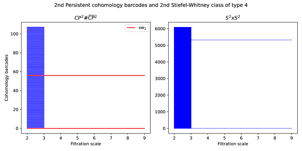
Figure 1: The second persistent cohomology barcodes and the second Stiefel–Whitney classes of type 4 at the maximum filtration scale computed for $\mathbb{CP}^{2}\#\overline{\mathbb{CP}}^{2}$ and $S^{2}\times S^{2}$. The horizontal axis represents the filtration scale, while the vertical axis indicates the persistent cohomology barcodes. Red barcodes correspond to cohomology classes whose sum yields the second Stiefel–Whitney class of type 4.

To construct the triangulation of $\mathbb{CP}^{2}\#\overline{\mathbb{CP}}^{2}$, we utilized the triangulation of $\mathbb{CP}^{2}$ from the Steenroder library [29]. We constructed filtered simplicial complexes from the triangulations of $\mathbb{CP}^{2}\#\overline{\mathbb{CP}}^{2}$ and $S^{2}\times S^{2}$, assigning filtration scales to simplices based on their dimensions. Using these filtered complexes, we computed persistent cohomology over $\mathbb{Z}/2$ and applied our algorithm to determine the first and second Stiefel–Whitney classes of type $4$ for each case. Since both manifolds are orientable, the first Stiefel–Whitney class is trivial in both cases. Figure 1 presents the results for the second persistent cohomology and the second Stiefel–Whitney class of type $4$ at the maximum filtration scale. As expected, both manifolds exhibit two independent second cohomology elements. However, for $\mathbb{CP}^{2}\#\overline{\mathbb{CP}}^{2}$, the sum of the cohomology classes corresponding to the two red barcodes yields a nontrivial second Stiefel–Whitney class, whereas for $S^{2}\times S^{2}$, the second Stiefel–Whitney class remains trivial. This result demonstrates the practical applicability of our algorithm.

6.2 Projective spaces of lines

In image analysis, topological data analysis offers a framework for capturing geometric and structural features that conventional pixel-based methods often fail to detect. By representing local image patches as high-dimensional point clouds, persistent homology enables the extraction of topological features that encode shape and texture information, complementing traditional feature extraction methods ([30, 31, 32, 33]).

Scoccola and Perea [10] proposed a method to compute characteristic classes of vector bundles by estimating tangent spaces using local PCA. In their approach, an image is partitioned into 250 patches of size $10\times 10$, which are then treated as the point cloud in $\mathbb{R}^{100}$. They computed the Stiefel–Whitney classes associated with these data points and argued that the result suggests that these patches are naturally embedded in the projective plane $\mathbb{RP}^{2}$, which has nontrivial first and second Stiefel–Whitney classes.

We used the LINES dataset from [10], which consists of the 250 patches discussed above. To reduce dimensionality while preserving essential structure, we applied principal component analysis (PCA) ([34]), projecting the dataset into $\mathbb{R}^{5}$. We then normalized each point to be in the unit sphere $S^{4}.$

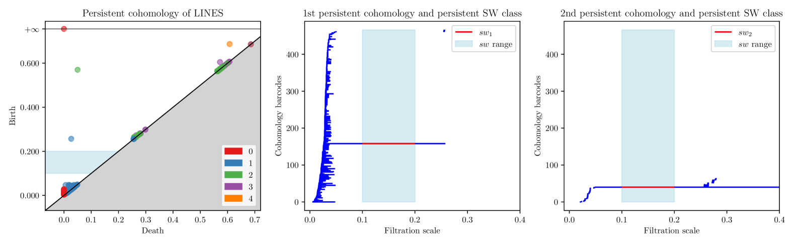
Figure 2: Persistent cohomology and persistent Stiefel–Whitney classes of type $2$ for the LINES dataset. The leftmost plot shows the persistent cohomology diagram over $\mathbb{Z}/2$. The middle and rightmost plots illustrate the first and second persistent barcodes and persistent Stiefel–Whitney classes of type $2$. The shaded regions indicate the filtration interval $[0.1,0.2]$ over which these classes satisfy the persistent Wu criterion.

From this processed point cloud, we constructed an alpha filtration and computed its persistent cohomology over $\mathbb{Z}/2$. Applying our proposed algorithm for computing persistent Stiefel–Whitney classes, we identified the first and second persistent Stiefel–Whitney classes of type $2$ over the filtration interval $[0.1,0.2]$. The results are presented in Figure 2. As expected, the two nontrivial barcodes in each dimension correspond to the computed persistent Stiefel–Whitney classes of type $2$.

6.3 Conformation space of cyclooctane

Cyclooctane ($\text{C}_{8}\text{H}_{16}$) is a flexible cyclic alkane with a complex conformation space due to its increased degrees of freedom. Topological data analysis has been applied to this space using persistent homology to analyze its geometric and topological structure. The conformation space of cyclooctane is nonmanifold, described as the union of a Klein bottle and $S^{2}$, which intersect along two disjoint circles ([29, 35, 36, 37]). Figure 3 illustrates the molecular structure of cyclooctane and its conformation space projected into $\mathbb{R}^{3}$.

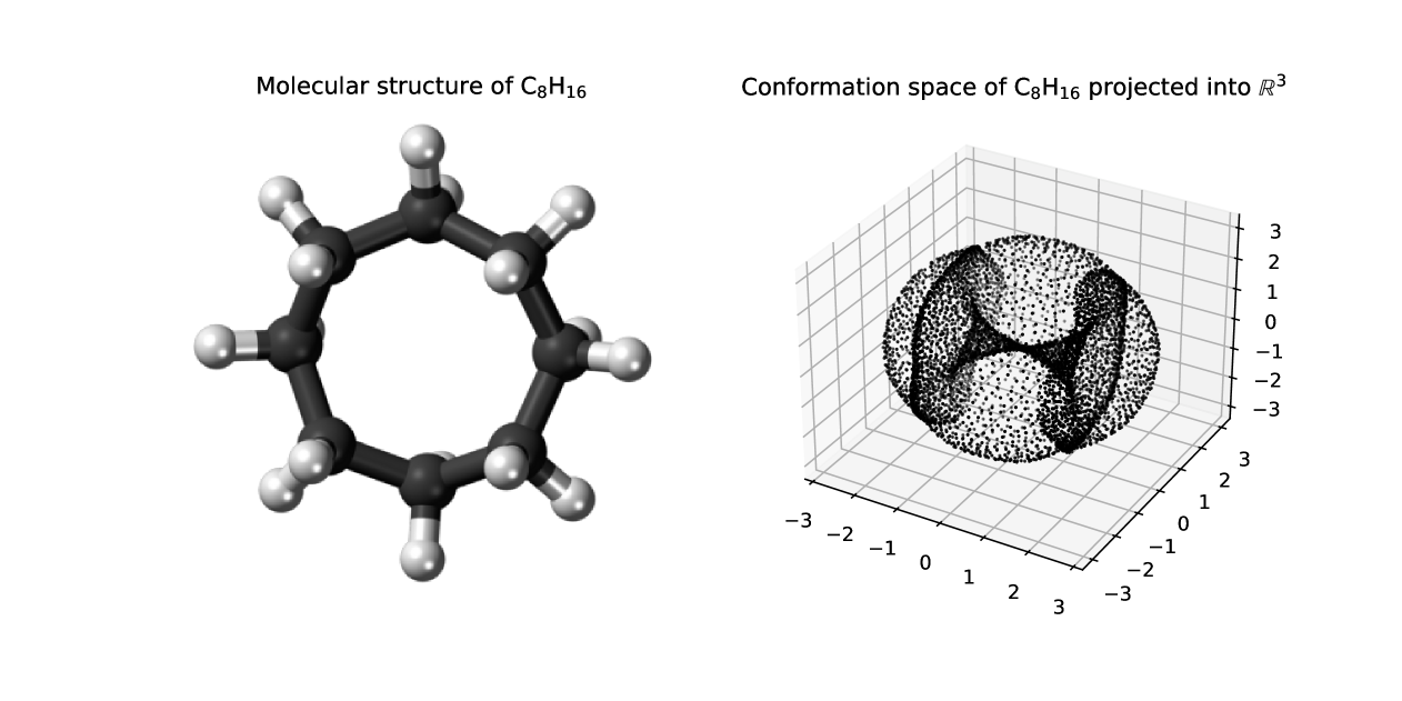
Figure 3: Molecular structure of cyclooctane ($\text{C}_{8}\text{H}_{16}$) and a point cloud sampled from its conformation space projected into $\mathbb{R}^{3}$. The conformation space consists of a Klein bottle and a 2-sphere intersecting along two disjoint circles.

Following [29], we started with 6040 points in $\mathbb{R}^{24}$ sampled from the conformation space of cyclooctane, originally introduced by [38]. Stolz et al. [39] applied a method based on local persistent cohomology to identify and remove 627 singular points. To further refine the structure, Lupo et al. [29] used the HDBSCAN clustering algorithm [40] to segment the remaining points into four clusters: one corresponding to an open subset of the Klein bottle and the other three forming subsets of $S^{2}$. Following these processes, we obtained a set of points sampled from the Klein bottle component of the conformation space.

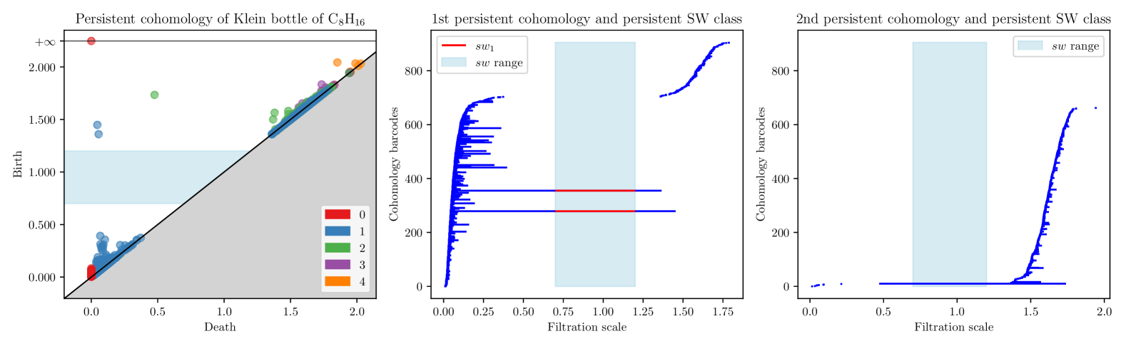
Figure 4: Persistent cohomology and persistent Stiefel–Whitney classes of type 2 for the point cloud sampled from the Klein bottle in the conformation space of cyclooctane. The leftmost plot shows the persistent cohomology diagram over $\mathbb{Z}/2$. The middle and rightmost plots illustrate the first and second persistent cohomology barcodes and the persistent Stiefel–Whitney classes of type 2. The shaded regions indicate the filtration interval $[0.7,1.2]$ over which these classes satisfy the persistent Wu criterion.

We selected $500$ points from the point cloud in the Klein bottle component and applied the UMAP algorithm [41] to embed them into $\mathbb{R}^{6}$. Figure 4 presents the persistent cohomology of the alpha filtration constructed from the point cloud in $\mathbb{R}^{6}$, together with the persistent Stiefel–Whitney classes of type $2$ computed over the filtration interval $[0.7,1.2]$. The first persistent Stiefel–Whitney class corresponds to the sum of two nontrivial cohomology classes, aligning with the nonorientability of the Klein bottle. In contrast, the second persistent Stiefel–Whitney class is trivial, indicating the absence of higher-order obstructions. These results are consistent with the known Stiefel–Whitney classes of the Klein bottle.

7 Conclusion

We proved that the persistent vector bundle is equivalent to the vector bundle filtration and that the persistent Stiefel–Whitney classes for both coincide. We defined the persistent Stiefel–Whitney class of type $n$ based on the Wu formula, which can be computed using cohomology barcode operations. We showed that if a filtration deformation retracts to an $n$-dimensional smooth manifold, then the persistent Stiefel–Whitney classes of type $n$ exist and correspond to the Stiefel–Whitney classes of $M$. We proposed an algorithm for computing the persistent Stiefel–Whitney class of type $n$, and demonstrated its effectiveness through numerical experiments.

Although our algorithm computes only the persistent Stiefel–Whitney classes, extending this approach to other important characteristic classes in a persistent setting, such as the Euler classes or Chern classes, is a promising direction for future research. One limitation of our approach is that it requires the use of Čech or Alpha filtrations, while the Rips filtration offers advantages in terms of time complexity. This is because the Nerve Lemma 4.1 holds only for the Čech or Alpha complex, and the Rips complex generates an excessive number of simplices hindering the efficient computation of the cup product and Steenrod squares. Thus, developing efficient methods for computing persistent characteristic classes within the Rips filtration would be a worthwhile pursuit for future study.

References

- [1] Manfredo P Do Carmo. Differential geometry of curves and surfaces: revised and updated second edition. Courier Dover Publications, 2016.
- [2] M Lee John. Introduction to Smooth Manifolds. Springer, 2024.
- [3] John Willard Milnor and James D Stasheff. Characteristic classes. Number 76 in Annals of Mathematics Studies. Princeton university press, 1974.
- [4] Dale Husemöller. Fibre bundles, volume 5. Springer, 1966.
- [5] Norman Steenrod. The topology of fibre bundles, volume 27. Princeton university press, 1999.
- [6] Edelsbrunner, Letscher, and Zomorodian. Topological persistence and simplification. Discrete & computational geometry, 28:511–533, 2002.
- [7] Afra Zomorodian and Gunnar Carlsson. Computing persistent homology. In Proceedings of the twentieth annual symposium on Computational geometry, pages 347–356, 2004.
- [8] Gunnar Carlsson. Topology and data. Bulletin of the American Mathematical Society, 46(2):255–308, 2009.
- [9] Raphaël Tinarrage. Computing persistent stiefel–whitney classes of line bundles. Journal of Applied and Computational Topology, 6(1):65–125, 2022.
- [10] Luis Scoccola and Jose A Perea. Approximate and discrete euclidean vector bundles. In Forum of Mathematics, Sigma, volume 11, page e20. Cambridge University Press, 2023.
- [11] Shiquan Ren. Persistent bundles over configuration spaces and obstructions for regular embeddings. arXiv preprint arXiv:2502.07476, 2025.
- [12] Nandakishore Kambhatla and Todd K Leen. Dimension reduction by local principal component analysis. Neural computation, 9(7):1493–1516, 1997.
- [13] Wen-Tsün Wu. Topologie-note sur les produits essentiels symetriques des espaces topologiques. COMPTES RENDUS HEBDOMADAIRES DES SEANCES DE L ACADEMIE DES SCIENCES, 224(16):1139–1141, 1947.
- [14] HB Aubrey. Persistent cohomology operations. PhD thesis, Duke University, 2011.
- [15] Allen Hatcher. Algebraic topology. Cambridge University Press, 2005.
- [16] Anibal M Medina-Mardones. New formulas for cup-i products and fast computation of steenrod squares. Computational Geometry, 109:101921, 2023.
- [17] Marco Contessoto, Facundo Mémoli, Anastasios Stefanou, and Ling Zhou. Persistent cup-length. arXiv preprint arXiv:2107.01553, 2021.
- [18] J Peter May. A concise course in algebraic topology. University of Chicago press, 1999.
- [19] Herbert Edelsbrunner and John Harer. Computational topology: an introduction. American Mathematical Soc., 2010.
- [20] Partha Niyogi, Stephen Smale, and Shmuel Weinberger. Finding the homology of submanifolds with high confidence from random samples. Discrete & Computational Geometry, 39:419–441, 2008.
- [21] Herbert Federer. Curvature measures. Transactions of the American Mathematical Society, 93(3):418–491, 1959.
- [22] Eddie Aamari, Jisu Kim, Frédéric Chazal, Bertrand Michel, Alessandro Rinaldo, and Larry Wasserman. Estimating the reach of a manifold. Electronic Journal of Statistics, 2019.
- [23] Raimund Seidel. The upper bound theorem for polytopes: an easy proof of its asymptotic version. Computational Geometry, 5(2):115–116, 1995.
- [24] Gene H Golub and Charles F Van Loan. Matrix computations. JHU press, 2013.
- [25] Clément Maria, Jean-Daniel Boissonnat, Marc Glisse, and Mariette Yvinec. The gudhi library: Simplicial complexes and persistent homology. In Mathematical Software–ICMS 2014: 4th International Congress, Seoul, South Korea, August 5-9, 2014. Proceedings 4, pages 167–174. Springer, 2014.
- [26] Dmitriy Morozov. Dionysus2: Library for computational topology, 2024. Accessed: 2025-02-14.
- [27] Dongwoo Gang. Persistent stiefel-whitney classes of tangent bundles : Computational examples. https://github.com/Dongwoo-Gang/sw-using-wu/tree/master, 2025. GitHub repository.
- [28] Daniel Huybrechts. Complex geometry: an introduction, volume 78. Springer, 2005.
- [29] Umberto Lupo, Anibal M Medina-Mardones, and Guillaume Tauzin. Persistence steenrod modules. Journal of Applied and Computational Topology, 6(4):475–502, 2022.
- [30] Gunnar Carlsson, Tigran Ishkhanov, Vin De Silva, and Afra Zomorodian. On the local behavior of spaces of natural images. International journal of computer vision, 76:1–12, 2008.
- [31] Yashbir Singh, Colleen M Farrelly, Quincy A Hathaway, Tim Leiner, Jaidip Jagtap, Gunnar E Carlsson, and Bradley J Erickson. Topological data analysis in medical imaging: current state of the art. Insights into Imaging, 14(1):58, 2023.
- [32] Felix Hensel, Michael Moor, and Bastian Rieck. A survey of topological machine learning methods. Frontiers in Artificial Intelligence, 4:681108, 2021.
- [33] James R Clough, Nicholas Byrne, Ilkay Oksuz, Veronika A Zimmer, Julia A Schnabel, and Andrew P King. A topological loss function for deep-learning based image segmentation using persistent homology. IEEE transactions on pattern analysis and machine intelligence, 44(12):8766–8778, 2020.
- [34] Hervé Abdi and Lynne J Williams. Principal component analysis. Wiley interdisciplinary reviews: computational statistics, 2(4):433–459, 2010.
- [35] Ernest L Eliel and Samuel H Wilen. Stereochemistry of organic compounds. John Wiley & Sons, 1994.
- [36] Ingrid Membrillo-Solis, Mariam Pirashvili, Lee Steinberg, Jacek Brodzki, and Jeremy G Frey. Topology and geometry of molecular conformational spaces and energy landscapes. arXiv preprint arXiv:1907.07770, 2019.
- [37] Henry Adams, Andrew Tausz, et al. Javaplex tutorial. Google Scholar, 27, 2011.
- [38] Shawn Martin, Aidan Thompson, Evangelos A Coutsias, and Jean-Paul Watson. Topology of cyclo-octane energy landscape. The journal of chemical physics, 132(23), 2010.
- [39] Bernadette J Stolz, Jared Tanner, Heather A Harrington, and Vidit Nanda. Geometric anomaly detection in data. Proceedings of the national academy of sciences, 117(33):19664–19669, 2020.
- [40] Ricardo JGB Campello, Davoud Moulavi, and Jörg Sander. Density-based clustering based on hierarchical density estimates. In Pacific-Asia conference on knowledge discovery and data mining, pages 160–172. Springer, 2013.
- [41] Leland McInnes, John Healy, and James Melville. Umap: Uniform manifold approximation and projection for dimension reduction. arXiv preprint arXiv:1802.03426, 2018.