From Paramagnet to Dipolar Topological Order via Duality and Dipolar SPT

Abstract

A scheme for the adaptive preparation of a topological state with dipole symmetry, dubbed the dipolar topological state (dTS), which serves as an example of translation symmetry-enriched topological phase, is proposed. The midcircuit state emerging during the preparation process is identified as a two-dimensional symmetry-protected topological (SPT) state protected by dipole bundle symmetry alongside charge and 1-form symmetries. The non-trivial boundary modes of the dipolar SPT state exhibiting the spontaneous breaking of charge and dipole bundle symmetries are analyzed. The duality map between the paramagnetic state and the dipolar topological state is established in the framework of the simultaneous gauging of two charge symmetries and one dipole symmetry that cannot be reduced as sequential gauging of the individual symmetry. Leveraging this duality, we work out the phase diagram of the dipolar topological state under perturbations by various transverse fields.

Introduction.— Fractons are elementary excitations that remain immobile on their own, realizable in three-dimensional systems but forbidden in strictly two-dimensional models [1, 2, 3]. Nevertheless, close analogues of fractons have been shown to emerge in certain two-dimensional lattice models where anyonic excitations are subject to mobility constraints forcing them to hop across multiple sites due to the presence of dipole conservation. The dipole constraint in turn has been shown to lead to interesting consequences such as position-dependent braiding statistics and system size-dependent ground state degeneracy (GSD) [4, 5, 6, 7, 8, 9, 10, 11, 12, 13, 14, 15, 16, 17, 18]. The rank-2 toric code (R2TC), a Higgsed descendant of rank-2 lattice gauge theory, provides an explicit realization of such mobility-constrained anyons due to dipole symmetry. The topological ground state emerging in R2TC and related models is hereby referred to as dipolar topological state (dTS). A characteristic feature of dTS is the permutation of anyon types under translation, which can be understood in the context of topological order enriched with translation symmetry [10]. The dTS thus joins a growing class of spin, diffusion, and strongly correlated boson/fermion models that incorporate dipole conservation [19, 20, 21, 22, 23, 24, 25, 26, 27, 28, 29, 30, 31, 32, 33].

Given the rapid theoretical advances in understanding dipole-conserving systems, the design of experimental realizations such as those in tilted optical lattice [34, 35, 36] is of increasing importance. For topological states such as the toric code, several measurement-based preparation schemes have been proposed [37, 38, 39, 40, 41, 42, 43, 44], building on foundational ideas of measurement-based quantum computation [45, 46]. Progress in implementing adaptive quantum circuits has been substantial in recent years [47, 48, 49, 50, 51], highlighting a promising route to realizing complex entangled states dynamically. The adaptive preparation schemes are closely related to various dualities between paramagnetic phases and topological phases [52, 39]. As we will show, the duality map to dTS involves a new type of duality mapping which we identify as the simultaneous gauging of charge and dipole symmetries.

\begin{overpic}[width=325.215pt]{stab_all.png} \put(-2.0,56.0){(a)} \put(72.0,56.0){(b)} \put(-2.0,25.0){(c)} \end{overpic}

Figure 1: (a) Three stabilizers of the R2TC. Red squares and lines indicate the vertex ($v$), the horizontal edge ($e_{\rm h}$), and the vertical edge ($e_{\rm v}$) about which the stabilizers are defined. (b) Qudits and the quantum circuit arrangements for the preparation of dCS. Two qudits are placed at the vertices and labeled $v_{l}$ and $v_{r}$, respectively. Single qudits are placed at the horizontal and vertical edges ($e_{\rm h}$, $e_{\rm v}$) as well as plaquette centers ($p$). The entanglers $(CZ)_{ab}$ and $(CZ)_{ab}^{\dagger}$ act on the two qudits connected by red and black lines, respectively, in accordance with the rule that the CZ operation involving one of the vertex qudits takes place between qudits of the same color. (c) Five stabilizers that realize the dCS. Red box indicates the stabilizer location.

In the case of preparing a ground state of the $\mathbb{Z}_{N}$ toric code, one starts with a two-dimensional cluster state (produced by a depth-2 local unitary circuit), then performs measurements on a subset of qudits located at the vertices and applies feedback on edge qudits based on the measurement outcomes. Generalizing the scheme, we propose a protocol for preparing the dTS state via the intermediate dipolar cluster state (dCS) serving as the midcircuit state. This is a symmetry-protected topological state protected by a dipole bundle symmetry [18], along with conventional charge and 1-form symmetries. Despite the higher complexity of the symmetries protecting the state, it can still be generated using a depth-2 local unitary circuit, making it experimentally realizable on a qutrit processor [53], for example . As an example of SPT, the dCS state hosts nontrivial boundary modes that spontaneously break both the global charge symmetry and dipole bundle symmetry. In the framework of duality, we show that the dTS represents an simple, yet nontrivial example of a topological state generated only through simultaneous gauging of charge and dipole symmetries, but not by sequential gauging of each symmetry, due to the fact that the charge and the dipole symmetries are intrinsically intertwined symmetries. Additionally, the new duality corresponding to the simultaneous gauging process enables us to analyze the phase transition of the dTS under transverse fields. The resulting transition serves as a dipolar generalization of the well-known confinement topological transition [55], thereby expanding the landscape of topological phase transitions to incorporate dipole symmetry.

Dipolar topological state.— A simple model that realizes the dTS is called the R2TC [6, 7, 8, 9, 10], which is a stabilizer model on a square lattice with three distinct stabilizers $S_{v}$, $S_{e_{\rm h}}$, and $S_{e_{\rm v}}$ shown in Fig. 1(a). Two qudits (of size $N$) occupy each vertex, and one qudit is at the plaquette center with $\mathbb{Z}_{N}$ Pauli operators $X$ and $Z$ obeying the commutation $ZX=\omega XZ$ ($\omega=e^{2\pi i/N}$) acting on them . The qudit $|s\rangle$, where $s\in\mathbb{Z}_{N}$ in the $Z$-basis, satisfies $X|s\rangle=|s+1\rangle$ and $Z|s\rangle=\omega^{s}|s\rangle$. There exist three 1-form symmetries, $g_{Z}^{1}$, $g_{Z}^{2}$, and $g_{Z}^{3}$, defined by a product of $Z$ operators along contractible or noncontractible loops, as well as three additional 1-form symmetries, $g_{X}^{1}$, $g_{X}^{2}$, and $g_{X}^{3}$, given by a product of $X$ operators. All of the six 1-form symmetries of R2TC act on vertices and plaquettes, but not on the edges where there are no quantum states. Their expressions can be found in [9] and in the Supplementary Materials (SM) [57].

Dipolar cluster state.— The dCS is defined on a square lattice with five qudits in a unit cell as in Fig. 1(b). To prepare the dCS, each qudit is initialized in the state $|\overline{0}\rangle$, which satisfies $X|\overline{0}\rangle=|\overline{0}\rangle$. A pairwise CZ (CZ^†) operation, defined by $(CZ)_{ab}|s_{a},s_{b}\rangle=\omega^{s_{a}s_{b}}|s_{a},s_{b}\rangle$, $s_{a,b}\in\mathbb{Z}_{N}$, takes place between two qudits connected by red (black) lines in Fig. 1(b). The CZ operation involving one of the vertex qudits takes place between qudits of the same color.

The paramagnetic state is stabilized by $X$ acting on each qudit. Therefore, the stabilizers that realize dCS are obtained by performing above-mentioned CZ operations, and invoking the identity $(CZ)_{ab}X_{a}(CZ)_{ab}^{\dagger}=X_{a}Z_{b}$. The five stabilizers $S^{\prime}_{e_{\rm h}}$, $S^{\prime}_{e_{\rm v}}$, $S^{\prime}_{v_{r}}$, $S^{\prime}_{p}$, and $S^{\prime}_{v_{l}}$ thus obtained are shown in Fig. 1(c).

Symmetries of dCS.—The dCS can be viewed as an SPT state protected by (i) two charge $\mathbb{Z}_{N}$ symmetries $g_{\rm h}$ and $g_{\rm v}$, (ii) a dipole bundle symmetry, and (iii) three 1-form symmetries, $g_{X}^{1}$, $g_{X}^{2}$, and $g_{X}^{3}$, which are also the three 1-form symmetries of R2TC.

The charge symmetry operators

$$g_{\rm h}:=\prod_{e_{\rm h}}X_{e_{\rm h}}=\prod_{e_{\rm h}}S^{\prime}_{e_{\rm h}},\quad g_{\rm v}:=\prod_{e_{\rm v}}X_{e_{\rm v}}=\prod_{e_{\rm v}}S^{\prime}_{e_{\rm v}}$$ (1)

are defined over the horizontal and vertical edges of the lattice, respectively.

The dipole symmetry should be defined differently for open and periodic boundary conditions. For an open boundary condition, if we exclude all incomplete stabilizers straddling the boundaries, the following modulated operator commutes with the Hamiltonian:

$$g_{\rm d} :=\prod_{e_{\rm h}}X_{e_{\rm h}}^{-y_{e_{\rm h}}}\prod_{e_{\rm v}}X_{e_{\rm v}}^{x_{e_{\rm v}}}$$

$$=\prod_{e_{\rm h}}(S_{e_{\rm h}}^{\prime})^{-y_{e_{\rm h}}}\prod_{e_{\rm v}}(S_{e_{\rm v}}^{\prime})^{x_{e_{\rm v}}},$$ (2)

where $x_{e_{\rm h}}$($x_{e_{\rm v}}$) and $y_{e_{\rm h}}$($y_{e_{\rm v}}$) refer to $x$ and $y$ coordinates of $e_{\rm h}$ ($e_{\rm v}$), respectively. For a $L_{x}\times L_{y}$ torus, one should define the dipole symmetry operator as

$$g_{\rm D}=g_{\rm d}^{N/\gcd(L_{x},L_{y},N)}.$$ (3)

When $\gcd(L_{x},L_{y},N)=1$, $g_{\rm D}=1$ and one loses the dipole symmetry. A unified understanding of the unique features of dipole symmetry comes from viewing it as an example of bundle symmetry [57, 29] rather than an ordinary global symmetry, and to view dCS as an SPT protected by such bundle symmetry along with global and 1-form symmetries.

A dipole symmetry operator similar to (2) can be defined for the usual cluster state in two dimensions, but it breaks down as a product of 1-form symmetries. In dCS, the dipole symmetry cannot be decomposed into 1-form symmetries, thus presenting itself as a unique new symmetry of the model.

Boundary modes of dCS.— The SPT hosts symmetry-protected boundary states arising from mutual anomalies among its governing symmetries. We identify the boundary modes of dCS for the case of a smooth horizontal boundary, where no $v_{r}$ qudits are present along the boundary . The case for more general boundary types is discussed in [57].

Using bulk stabilizer terms, the action of global symmetries on the dCS ground state $|\Psi\rangle$ can be shown to localize to the upper (u) and lower (l) boundaries as $g_{\rm a}|\Psi\rangle=g_{\rm a}^{\rm u}g_{\rm a}^{\rm l}|\Psi\rangle~({\rm a=h,v,d})$, where

$$g_{\rm h}^{\rm u} =\prod_{p,e_{\rm h}\in{\rm u}}Z_{p}^{\dagger}X_{e_{\rm h}},~~g_{\rm v}^{\rm u}=\prod_{v_{l}\in{\rm{\rm u}}}Z_{v_{l}},~~g_{\rm d}^{\rm u}=\prod_{v_{l}\in{\rm u}}Z_{v_{l}}^{x_{v_{l}}},$$ (4)

represent fractionalized symmetry operators on the upper boundary. (Similar operators exist for the lower boundary.) Assuming a semi-infinite system with only the upper boundary, the three operators derived in (4) serve as the symmetry operators of the edge-localized modes. They are independent symmetries, in the sense that no two operators can be related by the product of stabilizers in the bulk. Furthermore, these fractionalized operators have nontrivial commutation relations with the 1-form symmetries defined along the $y-$axis [57]:

$$g_{\rm h}^{\rm u}g_{X}^{2} =\omega g_{X}^{2}g_{\rm h}^{\rm u},~~g_{\rm v}^{\rm u}g_{X}^{1}=\omega g_{X}^{1}g_{\rm v}^{\rm u},~~g_{\rm d}^{\rm u}g_{X}^{3}=\omega g_{X}^{3}g_{\rm d}^{\rm u},$$ (5)

implying that the action by $g_{X}^{2},g_{X}^{1},g_{X}^{3}$ on a ground state toggles the eigenvalues of $g_{\rm h}^{\rm u},g_{\rm v}^{\rm u},g_{\rm d}^{\rm u}$ by $\omega$. Therefore, we have $N^{3}$ boundary zero modes labeled by $(q_{\rm h},q_{\rm v},q_{\rm d})\in\mathbb{Z}_{N}^{3}$. For a periodic lattice in the $x$ direction of length $L_{x}$, the proper symmetry operator is $g_{\rm d}^{N/\gcd(L_{x},N)}$ instead of $g_{\rm d}$, resulting in $N^{2}\gcd(L_{x},N)$-fold degeneracy.

This degeneracy can be seen more directly by constructing a symmetric boundary Hamiltonian. Let $U$ be the product of CZ and $\textrm{CZ}^{\dagger}$ operations that transform a paramagnetic state into the dCS state for a lattice with smooth boundary, and define $\overline{O}\,{:=}\,UOU^{\dagger}$. In this formalism, we can write $g_{\rm h}^{u}=\prod_{e_{\rm h}}\overline{X}_{e_{\rm h}}$ and $g_{\rm v}^{\rm u}=\prod_{v_{l}\in u}\overline{Z}_{v_{l}}$ and $g_{\rm d}^{\rm u}=\prod_{v_{l}\in u}\overline{Z}_{v_{l}}^{x_{v_{l}}}$ . One can show that the simplest symmetry-allowed local terms are

$$\overline{Z}_{e_{\rm h}}\overline{Z}_{e_{\rm h}+\hat{x}}^{\dagger},~~\overline{X}_{v_{l}-\hat{x}}(\overline{X}_{v_{l}}^{\dagger})^{2}\overline{X}_{v_{l}+\hat{x}}$$ (6)

and their conjugates. The boundary Hamiltonian $\sum_{e_{\rm h}}\overline{Z}_{e_{\rm h}}\overline{Z}_{e_{\rm h}+\hat{x}}^{\dagger}+{\rm h.c.}$ on horizontal edge qubits spontaneously breaks $g_{\rm h}^{u}$, resulting in an $N$-fold degeneracy. Similarly, the Hamiltonian $\sum_{v_{l}}\overline{X}_{v_{l}-\hat{x}}(\overline{X}_{v_{l}}^{\dagger})^{2}\overline{X}_{v_{l}+\hat{x}}+{\rm h.c.}$ breaks $g_{\rm v}^{u}$ and $g_{\rm d}^{u}$ ($(g_{\rm d}^{u})^{N/\gcd(L_{x},N)}$) with $N^{2}$ ($N\gcd(L_{x},N)$) degeneracy. Transverse field terms such as $\overline{X}_{e_{\rm h}}$ and $\overline{Z}_{v_{l}}$ that could lift the degeneracy at the boundary are forbidden by symmetry.

dCS to dTS by measurement.— After projecting all edge qudits in the dCS to the $X=+1$ eigenstate, remaining qudits at the vertices and plaquette centers form the ground state of R2TC. Indeed, the two stabilizers $S_{e_{\rm h}}^{\prime}$ and $S_{e_{\rm v}}^{\prime}$ commute with $X=+1$ measurement at the edges and reduce to $S_{e_{\rm h}}$ and $S_{e_{\rm v}}$ of R2TC, respectively. The collapsed state is an +1 eigenstate of $g_{X}^{1}$, $g_{X}^{2}$, and $g_{X}^{3}$, which are the symmetries of dCS that commute with the measurement. The remaining three stabilizers $S_{v_{r}}^{\prime}$, $S_{p}^{\prime}$, and $S_{v_{l}}^{\prime}$ in Fig. 1(c) by themselves do not commute with the measurements at the edges, but a carefully chosen product of them that equals $S_{v}$ of R2TC does . The collapsed state is $S_{v}=+1$ eigenstate regardless of the outcome of the edge-$X$ measurement. Other ground states of R2TC can be generated by further applying $g_{Z}^{1}$ through $g_{Z}^{3}$ on noncontractible loops to the collapsed state.

The symmetries of dCS that are operative at the edge qudits are closely associated with the conservation laws of R2TC. Invoking the relation $S_{e_{\rm h}}^{\prime}=X_{e_{\rm h}}S_{e_{\rm h}}$ and $S_{e_{\rm v}}^{\prime}=X_{e_{\rm v}}S_{e_{\rm v}}$ among the stabilizers of dCS and R2TC, and the fact that the symmetry operators of dCS defined in (1) and (3) become +1 in the dCS, it follows that

$$\prod_{e_{\rm h}}S_{e_{\rm h}}=1,~~~~~~~\prod_{e_{\rm v}}S_{e_{\rm v}}=1$$

$$\Bigl{(}\prod_{e_{\rm h}}(S_{e_{\rm h}})^{-y_{e_{\rm h}}}\prod_{e_{\rm v}}(S_{e_{\rm v}})^{x_{e_{\rm v}}}\Bigl{)}^{N/\gcd(L_{x},L_{y},N)}=1,$$ (7)

in the post-measurement state. The first two relations signify the conservation of two types of anyon charge and the third equation implies total dipole conservation. In short, the anyon charge and dipole conservations in the post-measurement topological model are a direct consequence of the charge and dipole symmetries of the pre-measurement dipolar SPT model.

Duality and simultaneous gauging.— One can decompose the Hilbert space of five qudits per unit cell into two parts: ($i$) ${\cal H}_{0}$ for two edge qudits, and $(ii)$ ${\cal H}_{1}$ for the remaining three qudits on the vertices and plaquette centers. Analogous to the Kramers-Wannier duality, a non-invertible duality transformation [61, 62] $K:{\cal H}_{0}\rightarrow{\cal H}_{1}$ can be constructed as shown in Fig. 2 using the operator [63, 64, 65]

$$K=\sum_{\{h\}}\omega^{\Phi(h)}|\{h_{v_{l}},h_{v_{r}},h_{p}\}\rangle\langle\{h_{e_{\rm h}},h_{e_{\rm v}}\}|,$$ (8)

where states are labeled in the $Z$-basis and the phase factor $\Phi(h)$ is given by

$$\Phi(h) =\sum_{h_{e_{\rm v}}}h_{e_{\rm v}}(h_{p,{\rm right}}-h_{p,{\rm left}}+h_{v_{l},{\rm bottom}}-h_{v_{l},{\rm top}})$$

$$+\sum_{h_{e_{\rm h}}}h_{e_{\rm h}}(h_{p,{\rm top}}-h_{p,{\rm bottom}}+h_{v_{r},{\rm left}}-h_{v_{r},{\rm right}}).$$

The top, bottom, left, right qudits with respect to a given edge qudit $e_{\rm h}$ or $e_{\rm v}$ are as indicated in Fig. 2(a).

Although ${\cal H}_{0}$ and ${\cal H}_{1}$ have different Hilbert space dimensions, the constrained spaces defined by

$${\cal H}^{\prime}_{0} =\{|\psi\rangle\in{\cal H}_{0}:g_{\rm h}|\psi\rangle=g_{\rm v}|\psi\rangle=g_{\rm D}|\psi\rangle=|\psi\rangle\}$$

$${\cal H}^{\prime}_{1} =\{|\psi\rangle\in{\cal H}_{1}:g_{X}^{1}|\psi\rangle=g_{X}^{2}|\psi\rangle=g_{X}^{3}|\psi\rangle=|\psi\rangle\}$$ (9)

share the same dimensionality equal to $N^{2L_{x}L_{y}-2}/\gcd(L_{x},L_{y},N)$, and the duality map between the constrained spaces becomes unitary. The choice of constraints is motivated by the observation that $g_{\rm h}$, $g_{\rm v}$ and $g_{\rm D}$ all become identity in ${\cal H}_{1}$ under $K$, and conversely $g_{X}^{1,2,3}$ map to identity in ${\cal H}_{0}$ under its inverse.

.

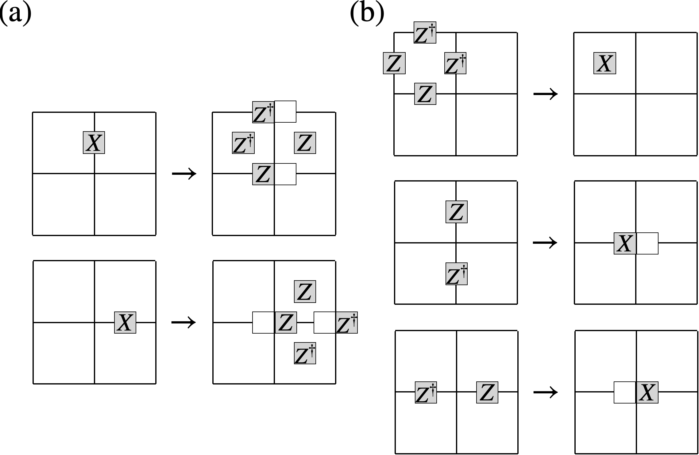
Figure 2: Duality transformation from edge qudits to vertex + plaquette qudits.

This duality transformation $K$, which maps the paramagnetic Hamiltonian to the R2TC, can be interpreted in the framework of symmetry gauging [44], specifically as the simultaneous gauging of two charge ($g_{\rm h}$ and $g_{\rm v}$) and one dipole symmetry ($g_{\rm D}$) . The necessity to perform simultaneous gauging arises from the intertwined nature of the dipole symmetry $g_{\rm D}$ with the charge symmetry $g_{\rm v}$ or $g_{\rm h}$ through the translation along the $x$-axis ($T_{x}$) or $y$-axis ($T_{y}$): $T_{x(y)}g_{\rm D}T_{x(y)}^{\dagger}=g_{\rm D}g_{\rm v(h)}^{N/\gcd(L_{x},L_{y},N)}$. Relevant gauge symmetry operators in the paramagnet-to-R2TC mapping are $S_{e_{\rm h}}’$ and $S_{e_{\rm v}}’$ in Fig. 1(c), which are the two stabilizers of the dCS defined on the edges. Their products generate the three global symmetries of dCS, $g_{\rm h}$, $g_{\rm v}$, and $g_{\rm D}$, given in (1)-(3). Therefore, all three symmetries are gauged when employing both $S_{e_{\rm h}}’$ and $S_{e_{\rm v}}’$ as gauge symmetry operators. Using only $S_{e_{\rm h}}’$ or $S_{e_{\rm v}}’$ results in gauging the $g_{\rm h}$ or $g_{\rm v}$ symmetry alone, which leads to a model distinct from R2TC. Note that both $S_{e_{\rm h}}’$ and $S_{e_{\rm v}}’$ act on the qudits at the plaquette centers, i.e. they share the plaquette-centered gauge field. As a result, gauging by $S_{e_{\rm h}}’$ and $S_{e_{\rm v}}’$ separately in a sequential manner is not possible. Therefore, this gauging process corresponds to the simultaneous gauging of $g_{\rm h}$, $g_{\rm v}$, and $g_{\rm D}$ . For comparison, an ordinary toric code is obtained by gauging only one type of gauge symmetry operator where there is no issue of simultaneous gauging. Finally, one can introduce gauging procedure for the mapping of paramagnet to two copies of the toric code; in that case the two gauging processes can be performed separately - see SM for details [57].

Quantum phase transitions.— Our goal now is to utilize the duality $K$ to understand the phase transition of R2TC, defined in the Hilbert space ${\cal H}_{1}$, subject to various transverse fields:

$$H(\lambda_{1},\lambda_{2},\lambda_{3})=-\sum_{v}S_{v}-\sum_{e_{\rm h}}S_{e_{\rm h}}-\sum_{e_{\rm v}}S_{e_{\rm v}}$$

$$~-\lambda_{1}\sum_{p}X_{p}-\lambda_{2}\sum_{v}X_{v_{l}}-\lambda_{3}\sum_{v}X_{v_{r}}+{\rm h.c.}.$$ (10)

The transverse field terms $X_{v_{l}}$, $X_{v_{r}}$, and $X_{p}$ generate quasiparticles (anyons) associated with $S_{e_{\rm v}}$, $S_{e_{\rm h}}$, and both $S_{e_{\rm v}}$ and $S_{e_{\rm h}}$, respectively. The anyons associated with $S_{e_{\rm h}}$ and $S_{v}$ exhibit nontrivial mutual statistics, as do those associated with $S_{e_{\rm v}}$ and $S_{v}$ [6].

The model $H(\lambda_{1},\lambda_{2},\lambda_{3})$ hosts four distinct phases $P_{1}$ through $P_{4}$. The $P_{1}$ is the regime in which the ground state remains in the same phase as R2TC, and occurs for small values of $\lambda_{\alpha}$, with $\alpha=1,2,3$. This is a topological phase characterized by the SSB of 1-form symmetries $g_{Z}^{1}$, $g_{Z}^{2}$, $g_{Z}^{3}$ or $g_{X}^{1}$, $g_{X}^{2}$, $g_{X}^{3}$, defined over a non-contractible loop.

The $P_{2}$ phase, realized for $\lambda_{2}\gg 1$, has finite average of $X_{v_{l}}$ and the concomitant condensation of the quasiparticles associated with $S_{e_{\rm v}}$ along with the confinement of quasiparticles associated with $S_{v}$. The fixed point of $P_{2}$, at $\lambda_{1},\lambda_{3}=0$ and $\lambda_{2}\to\infty$, has $S_{e_{v}}$ suppressed to zero and the remaining terms in the Hamiltonian acquire the local symmetry $l_{e_{\rm v}}$:

,

and two subsystem symmetries $s_{1}=\prod_{p\in C^{\rm v}}Z_{p}$ and $s_{2}=(\prod_{v\in C^{\rm v}}Z_{v_{r}}^{x_{v}})^{N/\gcd(L_{x},N)}$ along an arbitrary vertical loop $C^{\rm v}$ . These symmetry operators act non-trivially on the ground state manifold, resulting in the subextensive GSD growing as $N^{L_{x}}$ [57]. The $P_{2}$ phase is partially topological, as evidenced by the deconfinement of $S_{e_{\rm h}}$ quasiparticles and the existence of the corresponding Wilson loop operators $g_{X}^{2}$ (see Table 1) [57].

Similarly, the $P_{3}$ phase realized at $\lambda_{3}\gg 1$ is marked by the condensation of $S_{e_{\rm h}}$ quasiparticles (i.e. $\langle X_{v_{r}}\rangle\neq 0$) and the confinement of $S_{v}$ quasiparticles. This phase is obtained by applying a 90-degree rotation followed by a reflection across the $y$-axis to the $P_{2}$ phase, along with the exchange of qudits $v_{l}\leftrightarrow v_{r}$.

In the $P_{4}$ phase, both $S_{e_{\rm h}}$ and $S_{e_{\rm v}}$ quasiparticles are condensed and $S_{v}$ quasiparticles are confined, with finite expectation values of $X_{p}$, $X_{v_{l}}$, and $X_{v_{r}}$. This phase emerges under (i) $\lambda_{1}\gg 1$ with $\lambda_{2},\lambda_{3}>0$, or (ii) $\lambda_{2},\lambda_{3}\gg 1$ with $\lambda_{1}>0$. The ground state is unique.

Phase	GSD	Order parameter operators
$P_{1}$	$N^{3}c_{x}c_{y}c_{x,y}$	$g_{Z}^{1}$, $g_{Z}^{2}$, $g_{Z}^{3}$, $g_{X}^{1}$, $g_{X}^{2}$, $g_{X}^{3}$ (NC)
$P_{2}$	$N^{1+L_{x}}c_{y}$	$g_{Z}^{1}$, $g_{X}^{2}$ (NC)
$P_{3}$	$N^{1+L_{y}}c_{x}$	$g_{Z}^{2}$, $g_{X}^{1}$ (NC)
$P_{4}$	$1$	$X_{p}$, $X_{v_{l}}$, $X_{v_{r}}$
$P_{1}^{\prime}$	$1$	$X_{e_{\rm h}}$, $X_{e_{\rm v}}$
$P_{2}^{\prime}$	$N^{L_{x}}$	$X_{e_{\rm h}}$, $Z_{e_{\rm v}}$
$P_{3}^{\prime}$	$N^{L_{y}}$	$Z_{e_{\rm h}}$, $X_{e_{\rm v}}$
$P_{4}^{\prime}$	$N^{2}c_{x,y}$	$Z_{e_{\rm h}}$, $Z_{e_{\rm v}}$

Table 1: The characteristics of the phases $P_{1}$ through $P_{4}$ and $P_{1}^{\prime}$ through $P_{4}^{\prime}$. $c_{x}$, $c_{y}$, and $c_{x,y}$ denote $\gcd(L_{x},N)$, $\gcd(L_{y},N)$, and $\gcd(L_{x},L_{y},N)$, respectively. NC refers to operators defined on noncontractible loops.

We can dualize the Hamiltonian (10) by performing the inverse of the map given in Fig. 2 from ${\cal H}_{1}$ to ${\cal H}_{0}$:

$$H_{\rm dual}(\lambda_{1},\lambda_{2},\lambda_{3})=-\sum_{e_{\rm h}}X_{e_{\rm h}}-\sum_{e_{\rm v}}X_{e_{\rm v}}$$

$$~-\lambda_{1}\sum_{p}S_{p}^{\prime\prime}-\lambda_{2}\sum_{v_{l}}S_{v_{l}}^{\prime\prime}-\lambda_{3}\sum_{v_{r}}S_{v_{r}}^{\prime\prime}+{\rm h.c.},$$ (11)

where $S_{p}^{\prime\prime}$, $S_{v_{l}}^{\prime\prime}$, and $S_{v_{r}}^{\prime\prime}$ correspond to $S_{p}^{\prime}$, $S_{v_{l}}^{\prime}$, and $S_{v_{r}}^{\prime}$ with the $X$ operator omitted, respectively (they also appear on the left side of the arrow in Fig. 2(b)). The $S_{v}$ term in (10) drops out in the dual model . The four phases found in the dual Hamiltonian, labeled $P^{\prime}_{1}$ through $P^{\prime}_{4}$, are related to $P_{1}$ through $P_{4}$ phases by the $K$ duality.

The $P_{1}^{\prime}$ phase ($\lambda_{\alpha}\ll 1$) with a unique ground state is characterized by finite averages $\langle X_{e_{\rm h}}\rangle$ and $\langle X_{e_{\rm v}}\rangle$, and represents the dual of the dipolar topological phase of R2TC. The $P^{\prime}_{2}$ phase ($\lambda_{1},\lambda_{3}\ll 1\ll\lambda_{2}$) exhibits ferromagnetic order with finite $\langle Z_{e_{\rm v}}\rangle$ along each vertical chain for the $e_{\rm v}$ qudits while the $e_{\rm h}$ qudits remain paramagnetic with finite $\langle X_{e_{\rm h}}\rangle$. There is a sub-extensive GSD of $N^{L_{x}}$ with the factor $N$ arising from SSB of the subsystem symmetry $s_{1}^{\prime}=\prod_{e_{\rm v}\in C^{\rm v}}X_{e_{\rm v}}$ on each vertical chain. The $P^{\prime}_{3}$ phase ($\lambda_{1},\lambda_{2}\ll 1\ll\lambda_{3}$) is the $P^{\prime}_{2}$ phase with $e_{\rm v}$ and $e_{\rm h}$ qudits interchanged. The $P^{\prime}_{4}$ phase ($\lambda_{1}\gg 1$, $\lambda_{2},\lambda_{3}>0$ or $\lambda_{2},\lambda_{3}\gg 1$, $\lambda_{1}>0$) is understood as the SSB of two charge symmetries $g_{\rm v}$ and $g_{\rm h}$ and the dipole symmetry $g_{\rm D}$; it is characterized by finite $\langle Z_{e_{\rm h}}\rangle$ and $\langle Z_{e_{\rm v}}\rangle$.

The properties of the phases of $H(\lambda_{1},\lambda_{2},\lambda_{3})$ and $H_{\rm dual}(\lambda_{1},\lambda_{2},\lambda_{3})$ are summarized in Table 1. The dual Hamiltonian is defined on a smaller Hilbert space, has local order parameters to characterize phases as conventional SSB, and offers computational and conceptual simplicity over the original Hamiltonian.

Precise statements on the phase transitions can be made for the dual model at $\lambda_{1}=0$, where it reduces to a collection of $\mathbb{Z}_{N}$ transverse Ising chains oriented along each horizontal and vertical line. The second order phase transitions are expected on the self-dual lines $\lambda_{2}=1$ and $\lambda_{3}=1$, with the phase diagram given exactly as in Fig. 3(a). For the case $\lambda_{3}=0$, we obtain the phase diagram shown in Fig. 3(b) by numerical calculation of the dual Hamiltonian with $\mathbb{Z}_{2}$ degrees of freedom. The phase transition between $P_{1}$ and $P_{4}$ is identified as a first-order transition [57]. To conclude, rather precise statements on the various transitions away from the dipolar topological state can be made by judicious use of the duality argument and numerical calculation.

\begin{overpic}[width=208.13574pt]{Pd_a.png} \put(-1.0,78.0){(a)} \end{overpic}

\begin{overpic}[width=208.13574pt]{Pd_b.png} \put(-1.0,78.0){(b)} \end{overpic}

Figure 3: Phase diagram of perturbed R2TC at (a) $\lambda_{1}=0$, and (b) $\lambda_{3}=0$. First- and second-order phase transitions are depicted by dotted and solid lines, respectively.

Summary.— We proposed an adaptive preparation scheme for the topological state with dipole symmetry, using the rank-2 toric code as a specific example. The midcircuit state in the preparation process is a dipolar SPT state, protected by dipole bundle symmetry along with global charge and 1-form symmetries. A duality map relating the paramagnetic state to the dipolar topological state is analyzed, with the simultaneous gauging of two charge symmetries and one dipole symmetry as its interpretation. The duality map is then employed to identify various phases of the dipolar topological model perturbed by transverse fields.

More broadly, the simultaneous gauging of multiple symmetries may provide a useful framework for realizing novel exotic phases. On a related note, a clear decorated domain wall picture for the dipolar cluster state remains elusive, despite a well-established framework linking the SPT phase to a decorated domain wall picture [70, 62]. Further consideration for the symmetry classification of dipolar SPT states in two dimensions and the formulation of relevant background field theory may prove fruitful as well.

Acknowledgement.— We are grateful to Zijian Song, Yun-Tak Oh, Chanbeen Lee, Seunghun Lee, and Salvatore Pace for helpful discussions. J.Y.L. was supported by faculty startup grant at the University of Illinois, Urbana-Champaign. J.H.H. was supported by the National Research Foundation of Korea(NRF) grant funded by the Korea government(MSIT) (No. 2023R1A2C1002644). He acknowledges KITP, supported in part by the National Science Foundation under Grant No. NSF PHY-1748958.

I R2TC and its 1-form Symmetries

In this section, we provide a comprehensive summary of R2TC and its 1-form symmetries [9]. The R2TC Hamiltonian is given as

$$H=-\sum_{v}S_{v}-\sum_{e_{\rm h}}S_{e_{\rm h}}-\sum_{e_{\rm v}}S_{e_{\rm v}}+\textrm{h.c.}$$ (S1)

In this model, the mobility of anyons is constrained by the finite energy gap, and this restricted motion can be understood as a consequence of a dipole conservation of $\mathbb{Z}_{N}$ charge [6, 8, 9, 10]. For simplicity, let us assume $N$ being prime. To proceed, we define an anyon charge $c_{v}\in\mathbb{Z}_{N}$ for each vertex, which is associated with the value of the stabilizer $S_{v}=e^{i2\pi c_{v}/N}$ which is defined in the main Fig. 1(a). This anyon charge obeys the dipole conservation laws represented as

$$\sum_{v}x_{v}c_{v}\equiv\sum_{v}y_{v}c_{v}\equiv 0~{\rm mod}~N.$$ (S2)

Consequently, the movement of a non-trivial anyon $c_{v}\neq 0$ is permitted only if $x_{v}$ or $y_{v}$ increases by $N$.

On the other hand, the charges $c_{e_{\rm h}}$ and $c_{e_{\rm v}}$ associated with the stabilizer $S_{e_{\rm h}}$ and $S_{e_{\rm v}}$, respectively, have the following dipole conservation law:

$$\sum_{e_{\rm h}}y_{e_{\rm h}}c_{e_{\rm h}}+\sum_{e_{\rm v}}x_{e_{\rm v}}c_{e_{\rm v}}\equiv 0~{\rm mod}~N.$$ (S3)

Therefore, $c_{e_{\rm h}}$ can move in increments of $N$ steps along the $y$-axis, while $c_{e_{\rm v}}$ can move in increments of $N$ steps along the $x$-axis. In other directions, $c_{e_{\rm h}}$ and $c_{e_{\rm v}}$ can move without constraints. These mobility constraints also impose length restrictions on the 1-form symmetries.

\begin{overpic}[width=82.38885pt]{g123.png} \put(-5.0,112.0){(a)} \end{overpic}

\begin{overpic}[width=93.2267pt]{g456.png} \put(-5.0,100.0){(b)} \end{overpic}

Figure S1: (a) Examples of the $g_{Z}^{1}$, $g_{Z}^{2}$, and $g_{Z}^{3}$ when $N=3$. (b) Examples of $g_{X}^{1}$, $g_{X}^{2}$, and $g_{X}^{3}$ when $N=3$.

1-form $Z$ symmetries.

• $g_{Z}^{1}$ is defined on the loop composed of horizontal lines that intersect the vertices of the dual lattice and vertical lines intersecting the vertices of the lattice.

• $g_{Z}^{2}$ is defined on the loop composed of horizontal lines that intersect the vertices of the lattice and vertical lines that intersect the vertices of the dual lattice.

• $g_{Z}^{3}$ is defined on a loop composed of the edges of the lattice, where the lengths of the horizontal and vertical lines are constrained to be integer multiples of $N$. Due to the length restriction, $g_{Z}^{3}$ is better characterized as a sublattice 1-form symmetry [9].

For the non-contractible loop, the length restriction generally prevents $g_{Z}^{3}$ from being well-defined. However, it is possible for $(g_{Z}^{3})^{k}$ to be well-defined when $L_{x}k\mod N=0$ for horizontal loops and $L_{y}k\mod N=0$ for vertical loops. This can be interpreted as $g_{Z}^{3}$ winding $k$ times around the torus, with a total length of $kL_{x}$ for horizontal loops and $kL_{y}$ for vertical loops. The smallest value of $k$ equals ${\rm lcm}(L_{x},N)/N$ for horizontal loops and ${\rm lcm}(L_{y},N)/N$ for vertical loops. Examples of $g_{Z}^{1}$, $g_{Z}^{2}$, and $g_{Z}^{3}$ for $N=3$ is depicted in Fig. S1.

1-form $X$ symmetries.

• $g_{X}^{1}$ is defined on the fattened loop composed of fattened horizontal lines that intersect the vertices of the dual lattice and vertical lines that intersect the vertices of the lattice, where the length of the fattened horizontal lines be a multiple of $N$. This length restriction implies that for the non-contractible loop along the $x$-axis, $(g_{X}^{1})^{k}$ with $k=\mathrm{lcm}(L_{x},N)/N$ is a well-defined symmetry.

• $g_{X}^{2}$ is defined on the fattened loop composed of horizontal lines passing through the vertices of the lattice and fattened vertical lines intersecting the vertices of the dual lattice, where the length of the fattened vertical lines be a multiple of $N$. This length restriction implies that for the non-contractible loop along the $y$-axis, $(g_{X}^{2})^{k}$ with $k=\mathrm{lcm}(L_{y},N)/N$ is a well-defined symmetry.

• $g_{X}^{3}$ is defined on the fattened loop composed of the fattened edges of the dual lattice.

Examples of $g_{X}^{1}$, $g_{X}^{2}$, and $g_{X}^{3}$ for $N=3$ are depicted in Fig. S1(b).

The 1-form symmetries defined on non-contractible loops are logical operators that act on the degenerate ground state manifold. As previously noted, while some 1-form symmetries may not be well-defined on non-contractible loops, their powers may be well-defined. As the number of logical operators depends on the lattice size, the ground state degeneracy also depends on the lattice size. We refer to the GSD analysis using logical operators in [9].

Figure S2: $g_{X}^{1}(1)$, $g_{X}^{2}$, and $g_{X}^{3}$ defined along the $y$-axis with a smooth horizontal boundary for $N=3$

Finally, to aid in the understanding of (5) in the main text, Fig. S2 presents $g_{X}^{1}(1)$, $g_{X}^{2}$, and $g_{X}^{3}$ defined along the $y$-axis with a smooth horizontal boundary for $N=3$. Only $g_{X}^{1}(x_{v_{l}})$ is position-dependent and is generally expressed as

$$g_{X}^{1}(x_{v_{l}})=\prod_{x_{v_{l}}}X_{v_{l}}(X_{v_{l}}X_{v_{l}}^{\dagger})^{x_{v_{l}}}.$$ (S4)

II Dipole bundle symmetry

In this section, we provide a rigorous definition of the dipole bundle symmetry in two dimensions. The concept of the bundle symmetry was introduced in an earlier work on the dipolar SPT chain in one dimension [29]. The dipole bundle symmetry of the dCS, defined on a patch $A_{\alpha}$ enclosed by a contractible loop and denoted as $g_{b}(A_{\alpha})$, is expressed as:

$$g_{\rm b}(A_{\alpha}) :=\prod_{e_{\rm h}\in A_{\alpha}}X_{e_{\rm h}}^{-y_{e_{\rm h}}}\prod_{e_{\rm v}\in A_{\alpha}}X_{e_{\rm v}}^{x_{e_{\rm v}}}$$

$$=\prod_{e_{\rm h}\in A_{\alpha}}(S_{e_{\rm h}}^{\prime})^{-y_{e_{\rm h}}}\prod_{e_{\rm v}\in A_{\alpha}}(S_{e_{\rm v}}^{\prime})^{x_{e_{\rm v}}}.$$ (S5)

The lattice, which can be defined under both open and periodic boundary conditions, is covered by multiple overlapping patches enclosed by contractible loops, satisfying $A_{\alpha}\cap A_{\beta}\neq\emptyset$ and $\bigcup_{\alpha}A_{\alpha}=\text{lattice}$. For a given patch $A_{\alpha}$, $g_{\rm b}(A_{\alpha})$ commutes with stabilizers that are fully supported inside $A_{\alpha}$, but not with those defined across its boundary. When the lattice is defined under open boundary condition, $A_{\alpha}$ can encompass the entire lattice and yield $g_{\rm b}(\text{lattice})=g_{\rm d}$.

This is a notable departure from conventional global symmetry and highlights that the dCS under open and periodic boundary condition are protected by the same symmetries. As mentioned in the main text, $g_{\rm D}$, defined on the torus, commutes with the dCS Hamiltonian; however, its expression varies with lattice size. Arguing that $g_{\rm D}$ is the symmetry that protects the state is inappropriate, as the short-range entangled nature of the dCS—characterized by the reduced density matrix or correlation functions—is independent of the lattice size. Moreover, $g_{\rm d}$ does not commute with the dCS Hamiltonian in general. Therefore, the dCS is most appropriately described as being protected by the dipole bundle symmetry $g_{\rm b}(A_{\alpha})$.

III Boundary modes of dCS for a rough boundary

As we have analyzed the exotic boundary modes for a smooth horizontal boundary, we can consider a rough horizontal boundary. Under the similar process, the symmetry-allowed local boundary operators for a rough horizontal boundary are $\overline{X}_{p}\overline{X}_{p+\hat{x}}^{\dagger}$ and $\overline{Z}_{e_{\rm v}-\hat{x}}(\overline{Z}_{e_{\rm v}}^{\dagger})^{2}\overline{Z}_{e_{\rm v}+\hat{x}}$, where

.

These two terms commute and can coexist on the same boundary. The interaction term $\overline{X}_{p}\overline{X}_{p+\hat{x}}^{\dagger}$ induces SSB of the $\mathbb{Z}_{N}$ symmetry $g_{\rm h}$. Conversely, the interaction $\overline{Z}_{e_{\rm v}-\hat{x}}(\overline{Z}_{e_{\rm v}}^{\dagger})^{2}\overline{Z}_{e_{\rm v}+\hat{x}}$ leads to SSB of the $\mathbb{Z}_{N}\times\mathbb{Z}_{N}$ ($\mathbb{Z}_{N}\times\mathbb{Z}_{\gcd(L_{x},N)}$) symmetry associated with $g_{\rm v}$ and $g_{\rm d}$ ($g_{\rm d}^{N/\gcd(L_{x},N)}$). Thus, the SSB characteristics for both smooth and rough horizontal boundaries are identical.

IV Gauging of two charge symmetries

In this section, we present the gauging of $g_{\rm h}$ and $g_{\rm v}$, which is equivalent to the duality transformation between paramagentic state to the ground state of two copies of toric code. This will provide a clearer understanding of how the duality transformation $K$ in the main text differs from the gauging of $g_{\rm h}$ and $g_{\rm v}$.

Starting with the Hamiltonian $H=-\sum_{e_{\rm h}}X_{e_{\rm h}}-\sum_{e_{\rm v}}X_{e_{\rm v}}+{\rm h.c.}$, the process of gauging $g_{\rm h}$ and $g_{\rm v}$ proceeds as follows. First, gauge symmetry operators are introduced:

.

Red squares indicate the horizontal edges ($e_{\rm h}$) and vertical edges ($e_{\rm v}$) around which the stabilizers are defined. These gauge symmetry operators satisfy $\prod_{e_{\rm h}}G_{e_{\rm h}}=g_{e_{\rm h}}$ and $\prod_{e_{\rm v}}G_{e_{\rm v}}=g_{e_{\rm v}}$. We note that both vertices and plaquette centers host two qudits, with the operator $Z$ in $G_{e_{\rm h}}$ and $G_{e_{\rm v}}$ acting on the right and left qudits, respectively. In other words, this gauging process can be interpreted as the introduction of two distinct gauge fields: one dedicated to gauging $g_{\rm h}$ and the other to gauging $g_{\rm v}$. Therefore, this gauging process can be systematically decomposed into the sequential gauging of $g_{\rm h}$ followed by the gauging of $g_{\rm v}$.

As $X_{e_{\rm h}}$ and $X_{e_{\rm v}}$ commute with $G_{e_{\rm h}}$ and $G_{e_{\rm v}}$, the resulting total Hamiltonian, which is gauge-invariant, is given by:

$$H=-\sum_{e_{\rm h}}X_{e_{\rm h}}-\sum_{e_{\rm v}}X_{e_{\rm v}}-J_{1}(\sum_{e_{\rm h}}G_{e_{\rm h}}+\sum_{e_{\rm v}}G_{e_{\rm v}})-J_{2}(\sum_{e_{\rm h}}A_{e_{\rm h}}+\sum_{e_{\rm v}}A_{e_{\rm v}})+h.c.,$$ (S6)

where the operators $A_{e_{\rm h}}$ and $A_{e_{\rm v}}$ are

,

and are introduced to enforce the zero-flux constraints. Red lines indicate the horizontal edges ($e_{\rm h}$) and vertical edges ($e_{\rm v}$) around which the stabilizers are defined. Since under the transformation $G_{e_{\rm h}}\to X_{e_{\rm h}}$ and $G_{e_{\rm v}}\to X_{e_{\rm v}}$, the Hamiltonian $H$ remains invariant, applying the transformed gauge symmetry $X_{e_{\rm h}}=X_{e_{\rm v}}=+1$ results in the gauged Hamiltonian simplifying to two copies of the toric code. This gauging process can be implemented as an adaptive quantum circuit by constructing the stabilizers $G_{e_{\rm h}}$ and $G_{e_{\rm v}}$ through the application of unitary gates and the measurement of $e_{\rm h}$ and $e_{\rm v}$ qudits [39].

Note that although these two distinct gauging methods—gauging two charge symmetries and simultaneously gauging two charge symmetries along with one dipole symmetry—yield different lattice models, namely two copies of the toric code and dTS, respectively, the two copies of the toric code can be transformed into dTS by applying a projection onto the plaquette qubits [9]. In other words, simultaneous gauging can be implemented through two distinct approaches: (i) an adaptive quantum circuit that directly corresponds to simultaneous gauging, or (ii) an adaptive quantum circuit that first performs the gauging of two charge symmetries, followed by a projection.

Lastly, we clarify the nuanced distinction between the concept of simultaneous gauging in [71, 65] and the one introduced here. In [71, 65], a single gauge symmetry operator generates two distinct global symmetries, meaning that the gauge symmetry operator simultaneously gauges both global symmetries. In contrast, our approach, as discussed in the main text, involves two distinct gauge symmetry operators that share the same gauge field. Consequently, all symmetries associated with these gauge symmetry operators are simultaneously gauged. These two cases can both be regarded as instances of simultaneous gauging, as they involve gauge symmetry operator(s) that share a gauge field and are associated with multiple symmetries.

V Ground State Degeneracy of $P_{2}$ Phase

In this section, we will rigorously derive the ground state degeneracy (GSD) of the $P_{2}$ phase Hamiltonian under the periodic boundary condition at the fixed point of $P_{2}$, where $\lambda_{1},\lambda_{3}=0$ and $\lambda_{2}\to\infty$. Here, we consider two distinct approaches to calculating the GSD: (i) counting the number of independent stabilizer identities, and (ii) counting the number of independent operations that generate distinct ground states.

To implement the first method, the underlying logical framework is as follows. At the fixed point, the ground state corresponds to the +1 eigenstate of the operators $(X_{v_{l}},S_{v},S_{e_{\rm h}})$. Given that $X_{v_{l}}=1$ for all $v_{l}$ qudits, the effective Hamiltonian can be described in terms of the stabilizers $S_{v}^{P_{2}}$ and $S_{e_{\rm h}}$, where $S_{v}^{P_{2}}$ is expressed as

.

This formulation is applicable within the reduced Hilbert space $\{|h_{v_{r}},h_{p}\rangle\}$. The stabilizer $S_{e_{\rm h}}$ corresponds to the plaquette term of the $\mathbb{Z}_{N}$ toric code. Consequently, it satisfies a single identity, expressed as $\prod_{e_{\rm h}}S_{e_{\rm h}}=1$. The identities associated with $S_{v}^{P_{2}}$ are

$$\prod_{v\in C^{\rm v}}S_{v}^{P_{2}}=1,~~~~~~~~~\prod_{v\in C^{\rm v}}(S_{v}^{{P_{2}}})^{y_{v}N/\gcd(L_{y},N)}=1,$$ (S7)

where $C^{\rm v}$ is a vertical line. Therefore the GSD of the $P_{2}$ phase Hamiltonian is $N^{1+L_{x}}\gcd(L_{y},N)$.

To implement the second method, we first examine the ground state of the $P_{2}$ phase Hamiltonian, which is characterized as the +1 eigenstate of $S_{v}^{P_{2}}$’s:

$$|\psi\rangle=\prod_{e_{\rm h}}(1+S_{e_{\rm h}}+S_{e_{\rm h}}^{2}+\cdots+S_{e_{\rm h}}^{N-1})|\overline{0}\rangle,$$ (S8)

where $|\overline{0}\rangle$ is a +1 eigenstate of $X$ for every qudit. There are four distinct operations that yield different ground states. Two of these operations, $\prod_{p\in C^{\rm h}}Z_{p}$ and $\prod_{v_{r}\in C^{\rm v}}Z_{v_{r}}$, are effectively analogous to the Wilson loop operators in the toric code. Here, $C^{\rm h}$ refers the horizontal line. The contributions of these operations to the GSD are calculated to be $N$ and $N$, respectively. The remaining two operations are $\prod_{p\in C^{\rm v}}Z_{p}$ and $\prod_{v_{l}\in C^{\rm v}}Z_{v_{l}}^{y_{v_{l}}N/\gcd(L_{y},N)}$. Notably, two operators of the form $\prod_{v_{l}\in C^{\rm v}}Z_{v_{l}}^{y_{v_{l}}N/\gcd(L_{y},N)}$, defined on different vertical lines, are related through the product of $S_{e_{\rm h}}$ and $\prod_{p\in C^{\rm v}}Z_{p}$. Consequently, a straightforward counting of the contributions to the GSD from these two operations yields factors of $N^{L_{x}}$ and $\gcd(L_{y},N)$, respectively. However, not all of $\prod_{p\in C^{\rm v}}Z_{p}$ operations are independent. First of all, the product of $S_{e_{\rm h}}$, $\prod_{e_{\rm h}}S_{e_{\rm h}}^{-y_{{e_{\rm h}}}N/\gcd(L_{y},N)}$ is equivalent to $\prod_{p}Z_{p}^{N/\gcd(L_{y},N)}$, which means $\prod_{p}Z_{p}^{N/\gcd(L_{y},N)}$ is not the operation that give different ground state. Therefore, $N^{L_{x}}$ should be divided by $\gcd(L_{y},N)$. Furthermore, consider the $\prod_{p}Z_{p}$, which can be obtained by the product of $\prod_{p\in C^{\rm v}}Z_{p}$. This operation is equivalent to $\prod_{p\in C^{\rm h}}Z_{p}^{L_{y}}$, using the $S_{e_{\rm h}}$ operations. In number theory, it is well known that the least value of $nL_{y}\mod N$ is $\gcd(L_{y},N)$, where $n$ is a natural number. This means that when $\gcd(L_{y},N)=1$, the operation $\prod_{p\in C^{\rm h}}Z_{p}$, which was considered to contribute $N$ to the ground state, is in fact fully derivable from other operations and does not contribute at all. Therefore, in general, we can conclude that $\prod_{p\in C^{\rm h}}Z_{p}$ contributes $\gcd(L_{y},N)$ to the GSD. Collecting all contributions, this leads to $N^{1+L_{x}}\gcd(L_{y},N)$, which matches the result obtained using the first method.

For the last, we consider another ground state of the $P_{2}$ phase Hamiltonian, which is characterized as the +1 eigenstate of $S_{e_{\rm h}}$’s:

$$|\psi\rangle=\prod_{v}(1+S_{v}^{P_{2}}+(S_{v}^{P_{2}})^{2}+\cdots+(S_{v}^{P_{2}})^{N-1})|0\rangle,$$ (S9)

and try the similar analysis, where $|0\rangle$ is +1 eigenstate of every $Z$. There exists a local symmetry denoted by $l_{e_{\rm v}}$, where $l_{e_{\rm v}}$ and $l_{e_{\rm v}-\hat{y}}$ represent equivalent operations connected by $S_{v}^{P_{2}}$. Consequently, for each vertical line, there is one operation of $l_{e_{\rm v}}$. Additionally, another identity arises from the relation $\prod_{e_{\rm v}\in C^{\rm h}}l_{e_{\rm v}}^{L_{y}}$ is effectively equivalent to $\prod_{e_{\rm h}}l_{e_{\rm v}}=1$. Leveraging number theory, we deduce that $\prod_{e_{\rm v}\in C^{\rm h}}l_{e_{\rm v}}^{\gcd(L_{y},N)}=1$, implying that the contribution of the local symmetry is $N^{L_{x}-1}\gcd(L_{y},N)$. The remaining two symmetries, $\prod_{p\in C^{\rm v}}X_{p}$ and $\prod_{v_{r}\in C^{\rm h}}Z_{v_{r}}$, are analogous to Wilson loop operators in the toric code. Their contributions are $N$ and $N$, respectively, as the local symmetry connecting these symmetries across different loops has been fully accounted for. Thus, the GSD is determined to be $N^{1+L_{x}}\gcd(L_{y},N)$ once more.

VI Details of Numerical calculations

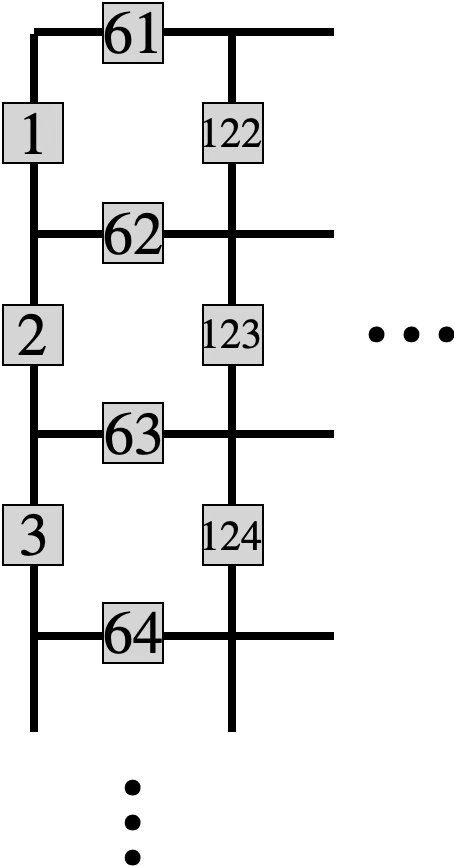
Figure S3: Labeling of the qudits of a lattice structure with dimensions $L_{x}=10$ and $L_{y}=60$. The numbering follows a column-major order, with labels increasing sequentially as you move downward within each column of qudits before progressing to the next column of qudits.

The numerical calculations of $H_{\rm dual}$ with $\mathbb{Z}_{2}$ degrees of freedom were performed employing a quasi-1D implementation of the density matrix renormalization group algorithm using matrix product states. We selected a lattice structure with dimensions $L_{x}=10$ and $L_{y}=60$, comprising $2$ qudits per unit cell under open boundary condition. The qudits were labeled as illustrated in Fig. S3. Key parameters included a cutoff of $10^{-9}$, a maximum bond dimension of $50$, and an energy tolerance of $10^{-9}$. The choice of $L_{y}=60$ was sufficient to attain the critical point within the range $1<\lambda_{2}<1.1$ under the condition $\lambda_{1}=\lambda_{3}=0$. Since $L_{y}=60$ is already considerably large to execute the quasi-1D calculation, and given the exponential growth of the bond dimension with increasing $L_{y}$, which is inherent to the quasi-1D implementation, obtaining the exact result becomes computationally challenging. Therefore, we selected $L_{x}=10$ to ensure computational feasibility. As a potential avenue for future research, one could explore the use of projected entangled pair states to achieve a more precise determination of the phase diagram.

Additionally, we present graphs derived from the numerical calculations of the expectation values of $Z_{e_{\rm h}}$ and $Z_{e_{\rm v}}$, aimed at identifying the critical points for various values of $\lambda_{1}$, $\lambda_{2}$, and $\lambda_{3}$. We show three specific cases: $\lambda_{1}=\lambda_{3}=0$ [Fig. S4(a)], $\lambda_{2}=0.3,\lambda_{3}=0$ [Fig. S4(b)], and $\lambda_{2}=0.8,\lambda_{3}=0$ [Fig. S4(c)], which illustrate the phase transitions between $P_{1}$ and $P_{3}$, $P_{1}$ and $P_{4}$, and $P_{1}$, $P_{2}$, and $P_{4}$, respectively. Based on the numerical results, we anticipate that the phase transition between $P_{1}$ and $P_{4}$ is of first order, whereas the other transitions correspond to the second order phase transitions.

\begin{overpic}[width=138.76157pt]{cut_1.png} \put(-3.0,75.0){(a)} \end{overpic}

\begin{overpic}[width=138.76157pt]{cut_03.png} \put(-3.0,75.0){(b)} \end{overpic}

\begin{overpic}[width=138.76157pt]{cut_08.png} \put(-3.0,75.0){(c)} \end{overpic}

Figure S4: The graphs of the absolute values of $\langle Z_{e_{\rm h}}\rangle$ and $\langle Z_{e_{\rm v}}\rangle$ are presented for the following cases: (a) $\lambda_{1}=\lambda_{3}=0$, (b) $\lambda_{2}=0.3,\lambda_{3}=0$, and (c) $\lambda_{2}=0.8,\lambda_{3}=0$. The dots represent the values obtained from the numerical simulations.

References

- Nandkishore and Hermele [2019] R. M. Nandkishore and M. Hermele, Fractons, Annual Review of Condensed Matter Physics 10, 295 (2019), https://doi.org/10.1146/annurev-conmatphys-031218-013604 .
- Pretko et al. [2020] M. Pretko, X. Chen, and Y. You, Fracton phases of matter, International Journal of Modern Physics A 35, 2030003 (2020), https://doi.org/10.1142/S0217751X20300033 .
- Gromov and Radzihovsky [2024] A. Gromov and L. Radzihovsky, Colloquium: Fracton matter, Rev. Mod. Phys. 96, 011001 (2024).
- Ma et al. [2018] H. Ma, M. Hermele, and X. Chen, Fracton topological order from the Higgs and partial-confinement mechanisms of rank-two gauge theory, Phys. Rev. B 98, 035111 (2018).
- Bulmash and Barkeshli [2018] D. Bulmash and M. Barkeshli, Higgs mechanism in higher-rank symmetric U(1) gauge theories, Phys. Rev. B 97, 235112 (2018).
- Oh et al. [2022a] Y.-T. Oh, J. Kim, E.-G. Moon, and J. H. Han, Rank-2 toric code in two dimensions, Phys. Rev. B 105, 045128 (2022a).
- Pace and Wen [2022] S. D. Pace and X.-G. Wen, Position-dependent excitations and UV/IR mixing in the rank-2 toric code and its low-energy effective field theory, Phys. Rev. B 106, 045145 (2022).
- Oh et al. [2022b] Y.-T. Oh, J. Kim, and J. H. Han, Effective field theory of dipolar braiding statistics in two dimensions, Phys. Rev. B 106, 155150 (2022b).
- Oh et al. [2023] Y.-T. Oh, S. D. Pace, J. H. Han, Y. You, and H.-Y. Lee, Aspects of rank-2 gauge theory in dimensions: Construction schemes, holonomies, and sublattice one-form symmetries, Phys. Rev. B 107, 155151 (2023).
- Kim et al. [2023] J. Kim, Y.-T. Oh, D. Bulmash, and J. H. Han, Unveiling UV/IR Mixing via Symmetry Defects: A View from Topological Entanglement Entropy (2023), arXiv:2310.09425 [cond-mat.str-el] .
- Watanabe et al. [2023] H. Watanabe, M. Cheng, and Y. Fuji, Ground state degeneracy on torus in a family of toric code, Journal of Mathematical Physics 64, 051901 (2023).
- Ebisu [2023] H. Ebisu, Symmetric higher rank topological phases on generic graphs, Phys. Rev. B 107, 125154 (2023).
- Delfino et al. [2023a] G. Delfino, C. Chamon, and Y. You, 2D Fractons from Gauging Exponential Symmetries (2023a), arXiv:2306.17121 [cond-mat.str-el] .
- Gorantla et al. [2023a] P. Gorantla, H. T. Lam, N. Seiberg, and S.-H. Shao, Gapped lineon and fracton models on graphs, Phys. Rev. B 107, 125121 (2023a).
- Delfino et al. [2023b] G. Delfino, W. B. Fontana, P. R. S. Gomes, and C. Chamon, Effective fractonic behavior in a two-dimensional exactly solvable spin liquid, SciPost Phys. 14, 002 (2023b).
- Huang [2023] X. Huang, A Chern-Simons theory for dipole symmetry, SciPost Phys. 15, 153 (2023).
- Ebisu et al. [2024] H. Ebisu, M. Honda, and T. Nakanishi, Multipole and fracton topological order via gauging foliated symmetry protected topological phases, Phys. Rev. Res. 6, 023166 (2024).
- Han [2024] J. H. Han, Dipolar background field theory and dipolar braiding statistics, Phys. Rev. B 109, 235127 (2024).
- Sachdev et al. [2002] S. Sachdev, K. Sengupta, and S. Girvin, Mott insulators in strong electric fields, Physical Review B 66, 075128 (2002).
- Morningstar et al. [2020] A. Morningstar, V. Khemani, and D. A. Huse, Kinetically constrained freezing transition in a dipole-conserving system, Physical Review B 101, 214205 (2020).
- Sala et al. [2020] P. Sala, T. Rakovszky, R. Verresen, M. Knap, and F. Pollmann, Ergodicity breaking arising from Hilbert space fragmentation in dipole-conserving Hamiltonians, Physical Review X 10, 011047 (2020).
- Feldmeier et al. [2020] J. Feldmeier, P. Sala, G. De Tomasi, F. Pollmann, and M. Knap, Anomalous Diffusion in Dipole- and Higher-Moment-Conserving Systems, Phys. Rev. Lett. 125, 245303 (2020).
- Gromov et al. [2020] A. Gromov, A. Lucas, and R. M. Nandkishore, Fracton hydrodynamics, Phys. Rev. Res. 2, 033124 (2020).
- Grosvenor et al. [2022] K. T. Grosvenor, C. Hoyos, F. Peña-Benítez, and P. Surówka, Space-Dependent Symmetries and Fractons, Frontiers in Physics 9, 10.3389/fphy.2021.792621 (2022).
- Gorantla et al. [2022] P. Gorantla, H. T. Lam, N. Seiberg, and S.-H. Shao, Global dipole symmetry, compact Lifshitz theory, tensor gauge theory, and fractons, Phys. Rev. B 106, 045112 (2022).
- Sala et al. [2022] P. Sala, J. Lehmann, T. Rakovszky, and F. Pollmann, Dynamics in Systems with Modulated Symmetries, Phys. Rev. Lett. 129, 170601 (2022).
- Gorantla et al. [2023b] P. Gorantla, H. T. Lam, N. Seiberg, and S.-H. Shao, (2+1)-dimensional compact Lifshitz theory, tensor gauge theory, and fractons, Phys. Rev. B 108, 075106 (2023b).
- Pozderac et al. [2023] C. Pozderac, S. Speck, X. Feng, D. A. Huse, and B. Skinner, Exact solution for the filling-induced thermalization transition in a one-dimensional fracton system, Phys. Rev. B 107, 045137 (2023).
- Han et al. [2024a] J. H. Han, E. Lake, H. T. Lam, R. Verresen, and Y. You, Topological quantum chains protected by dipolar and other modulated symmetries, Phys. Rev. B 109, 125121 (2024a).
- Lake et al. [2022] E. Lake, M. Hermele, and T. Senthil, Dipolar Bose-Hubbard model, Phys. Rev. B 106, 064511 (2022).
- Zechmann et al. [2023] P. Zechmann, E. Altman, M. Knap, and J. Feldmeier, Fractonic Luttinger liquids and supersolids in a constrained Bose-Hubbard model, Phys. Rev. B 107, 195131 (2023).
- Lake et al. [2023] E. Lake, H.-Y. Lee, J. H. Han, and T. Senthil, Dipole condensates in tilted Bose-Hubbard chains, Phys. Rev. B 107, 195132 (2023).
- Han et al. [2024b] J. H. Han, E. Lake, and S. Ro, Scaling and Localization in Multipole-Conserving Diffusion, Phys. Rev. Lett. 132, 137102 (2024b).
- Guardado-Sanchez et al. [2020] E. Guardado-Sanchez, A. Morningstar, B. M. Spar, P. T. Brown, D. A. Huse, and W. S. Bakr, Subdiffusion and Heat Transport in a Tilted Two-Dimensional Fermi-Hubbard System, Phys. Rev. X 10, 011042 (2020).
- Scherg et al. [2021] S. Scherg, T. Kohlert, P. Sala, F. Pollmann, B. H. Madhusudhana, I. Bloch, and M. Aidelsburger, Observing non-ergodicity due to kinetic constraints in tilted Fermi-Hubbard chains, Nature Communications 12, 1 (2021).
- Zahn et al. [2022] H. Zahn, V. Singh, M. Kosch, L. Asteria, L. Freystatzky, K. Sengstock, L. Mathey, and C. Weitenberg, Formation of spontaneous density-wave patterns in DC driven lattices, Physical Review X 12, 021014 (2022).
- Hastings and Haah [2021] M. B. Hastings and J. Haah, Dynamically Generated Logical Qubits, Quantum 5, 564 (2021).
- Piroli et al. [2021] L. Piroli, G. Styliaris, and J. I. Cirac, Quantum Circuits Assisted by Local Operations and Classical Communication: Transformations and Phases of Matter, Phys. Rev. Lett. 127, 220503 (2021).
- Tantivasadakarn et al. [2024] N. Tantivasadakarn, R. Thorngren, A. Vishwanath, and R. Verresen, Long-Range Entanglement from Measuring Symmetry-Protected Topological Phases, Physical Review X 14, 021040 (2024).
- Verresen et al. [2022] R. Verresen, N. Tantivasadakarn, and A. Vishwanath, Efficiently preparing Schrödinger’s cat, fractons and non-Abelian topological order in quantum devices (2022), arXiv:2112.03061 [quant-ph] .
- Bravyi et al. [2022] S. Bravyi, I. Kim, A. Kliesch, and R. Koenig, Adaptive constant-depth circuits for manipulating non-abelian anyons (2022), arXiv:2205.01933 [quant-ph] .
- Lu et al. [2022] T.-C. Lu, L. A. Lessa, I. H. Kim, and T. H. Hsieh, Measurement as a Shortcut to Long-Range Entangled Quantum Matter, PRX Quantum 3, 040337 (2022).
- Aasen et al. [2022] D. Aasen, Z. Wang, and M. B. Hastings, Adiabatic paths of Hamiltonians, symmetries of topological order, and automorphism codes, Phys. Rev. B 106, 085122 (2022).
- Tantivasadakarn et al. [2023] N. Tantivasadakarn, R. Verresen, and A. Vishwanath, Shortest Route to Non-Abelian Topological Order on a Quantum Processor, Phys. Rev. Lett. 131, 060405 (2023).
- Briegel and Raussendorf [2001] H. J. Briegel and R. Raussendorf, Persistent Entanglement in Arrays of Interacting Particles, Phys. Rev. Lett. 86, 910 (2001).
- Raussendorf et al. [2005] R. Raussendorf, S. Bravyi, and J. Harrington, Long-range quantum entanglement in noisy cluster states, Phys. Rev. A 71, 062313 (2005).
- Pino et al. [2021] J. M. Pino, J. M. Dreiling, C. Figgatt, J. P. Gaebler, S. A. Moses, M. S. Allman, C. H. Baldwin, M. Foss-Feig, D. Hayes, K. Mayer, C. Ryan-Anderson, and B. Neyenhuis, Demonstration of the trapped-ion quantum CCD computer architecture, Nature 592, 209 (2021).
- Ryan-Anderson et al. [2021] C. Ryan-Anderson, J. G. Bohnet, K. Lee, D. Gresh, A. Hankin, J. P. Gaebler, D. Francois, A. Chernoguzov, D. Lucchetti, N. C. Brown, T. M. Gatterman, S. K. Halit, K. Gilmore, J. A. Gerber, B. Neyenhuis, D. Hayes, and R. P. Stutz, Realization of Real-Time Fault-Tolerant Quantum Error Correction, Phys. Rev. X 11, 041058 (2021).
- Córcoles et al. [2021] A. D. Córcoles, M. Takita, K. Inoue, S. Lekuch, Z. K. Minev, J. M. Chow, and J. M. Gambetta, Exploiting Dynamic Quantum Circuits in a Quantum Algorithm with Superconducting Qubits, Phys. Rev. Lett. 127, 100501 (2021).
- Foss-Feig et al. [2023] M. Foss-Feig, A. Tikku, T.-C. Lu, K. Mayer, M. Iqbal, T. M. Gatterman, J. A. Gerber, K. Gilmore, D. Gresh, A. Hankin, N. Hewitt, C. V. Horst, M. Matheny, T. Mengle, B. Neyenhuis, H. Dreyer, D. Hayes, T. H. Hsieh, and I. H. Kim, Experimental demonstration of the advantage of adaptive quantum circuits (2023), arXiv:2302.03029 [quant-ph] .
- Iqbal et al. [2024] M. Iqbal, N. Tantivasadakarn, R. Verresen, S. L. Campbell, J. M. Dreiling, C. Figgatt, J. P. Gaebler, J. Johansen, M. Mills, S. A. Moses, J. M. Pino, A. Ransford, M. Rowe, P. Siegfried, R. P. Stutz, M. Foss-Feig, A. Vishwanath, and H. Dreyer, Non-Abelian topological order and anyons on a trapped-ion processor, Nature 626, 505 (2024).
- Tantivasadakarn and Vijay [2020] N. Tantivasadakarn and S. Vijay, Searching for fracton orders via symmetry defect condensation, Phys. Rev. B 101, 165143 (2020).
- Blok et al. [2021] M. S. Blok, V. V. Ramasesh, T. Schuster, K. O’Brien, J. M. Kreikebaum, D. Dahlen, A. Morvan, B. Yoshida, N. Y. Yao, and I. Siddiqi, Quantum Information Scrambling on a Superconducting Qutrit Processor, Phys. Rev. X 11, 021010 (2021).
- Note [1] The dTS are typically realized for where refers to the local degrees of freedom.
- Tupitsyn et al. [2010] I. S. Tupitsyn, A. Kitaev, N. V. Prokof’ev, and P. C. E. Stamp, Topological multicritical point in the phase diagram of the toric code model and three-dimensional lattice gauge Higgs model, Phys. Rev. B 82, 085114 (2010).
- Note [2] These stabilizers are equivalent to those in [6, 10], up to qudit rotations, and are more elegant considering the duality interpretation.
- Kim et al. [2025] J. Kim, J. Y. Lee, and J. H. Han, Supplementary Information for “Adaptive Preparation of the Dipolar Topological State through Dipolar Symmetry-Protected Topological State”, Supplemental Material available at [URL] (2025), accessed: [Access Date].
- Note [3] If qudits are present, the boundary cannot be considered a genuine boundary, as the stabilizer remains well-defined along it.
- Note [4] for periodic boundary condition.
-
Note [5]
.
- Radicevic [2019] D. Radicevic, Spin Structures and Exact Dualities in Low Dimensions (2019), arXiv:1809.07757 [hep-th] .
- Yoshida [2016] B. Yoshida, Topological phases with generalized global symmetries, Physical Review B 93, 155131 (2016).
- Yan and Li [2024] H. Yan and L. Li, Generalized Kramers-Wanier Duality from Bilinear Phase Map (2024), arXiv:2403.16017 [cond-mat.str-el] .
- Parayil Mana et al. [2024] A. Parayil Mana, Y. Li, H. Sukeno, and T.-C. Wei, Kennedy-Tasaki transformation and noninvertible symmetry in lattice models beyond one dimension, Phys. Rev. B 109, 245129 (2024).
- Cao et al. [2024] W. Cao, L. Li, and M. Yamazaki, Generating lattice non-invertible symmetries, SciPost Physics 17, 10.21468/scipostphys.17.4.104 (2024).
- Note [6] We primarily focus on the torus; however, for a lattice with open boundary condition, the appropriate dipole symmetry is .
- Note [7] The term ‘simultaneous gauging’ was introduced in [65], and a related study can be found in [71]. We compare the gauging process in [65, 71] with the one introduced here; see Supplementary Material [57].
- Note [8] Under the open boundary condition, the expression of will be changed to .
- Note [9] The Hamiltonian and its dual will share the same phase diagram even without imposing the constraint, as the constraint used to reduce to ( to ) commute with the Hamiltonian ().
- Chen et al. [2014] X. Chen, Y.-M. Lu, and A. Vishwanath, Symmetry-protected topological phases from decorated domain walls, Nature Communications 5, 3507 (2014).
- Pace et al. [2025] S. D. Pace, G. Delfino, H. T. Lam, and Ömer M. Aksoy, Gauging modulated symmetries: Kramers-Wannier dualities and non-invertible reflections, SciPost Phys. 18, 021 (2025).
Supplementary Information for “From Paramagnet to Dipolar Topological Order via Duality and Dipolar SPT”
Jintae Kim1,2,∗, Jong Yeon Lee,3,†, and Jung Hoon Han1,‡
1Department of Physics, Sungkyunkwan University, Suwon 16419, South Korea
2Institute of Basic Science, Sungkyunkwan University, Suwon 16419, South Korea
3Physics Department and Insitute of Condensed Matter Theory, University of Illinois at Urbana-Champaign, Urbana, Illinois 61801, USA
(Dated: April 5, 2025)