Rapid quantum ground state preparation via dissipative dynamics

Abstract

Inspired by natural cooling processes, dissipation has become a promising approach for preparing low-energy states of quantum systems. However, the potential of dissipative protocols remains unclear beyond certain commuting Hamiltonians. This work provides significant analytical and numerical insights into the power of dissipation for preparing the ground state of non-commuting Hamiltonians. For quasi-free dissipative dynamics, including certain 1D spin systems with boundary dissipation, our results reveal a new connection between the mixing time in trace distance and the spectral properties of a non-Hermitian Hamiltonian, leading to an explicit and sharp bound on the mixing time that scales polynomially with system size. For more general spin systems, we develop a tensor network-based algorithm for constructing the Lindblad jump operator and for simulating the dynamics. Using this algorithm, we demonstrate numerically that dissipative ground state preparation protocols can achieve rapid mixing for certain 1D local Hamiltonians under bulk dissipation, with a mixing time that scales logarithmically with the system size. We then prove the rapid mixing result for certain weakly interacting spin and fermionic systems in arbitrary dimensions, extending recent results for high-temperature quantum Gibbs samplers to the zero-temperature regime. Our theoretical approaches are applicable to systems with singular stationary states, and are thus expected to have applications beyond the specific systems considered in this study.

I Introduction

Ground state preparation is one of the most important challenges in quantum many-body physics, quantum chemistry, and materials science. Quantum algorithms, such as quantum phase estimation (QPE), quantum singular value transformation (QSVT), adiabatic state preparation (ASP) and their variants [50, 28, 42, 43, 2, 25], offer a pathway to tackle challenging ground state preparation problems beyond the capabilities of classical computers. Dissipative dynamics, such as Lindblad dynamics, provides a distinct approach to state preparation. This approach evolves the system density matrix under engineered dissipation and Hamiltonian dynamics, and encodes the target state as the steady-state solution of the Lindblad master equation.

Dissipative techniques, and state preparation methods employing mid-circuit measurements in general, have been widely applied to prepare matrix product states, ground states of stabilizer codes, spin systems, and other states exhibiting long-range entanglement [37, 70, 76, 16, 74, 44, 26, 34]. Compared to traditional unitary quantum algorithms as well as adiabatic algorithms, dissipative approaches offer certain inherent robustness to noise, and may bypass the need for complex initialization procedures, making them attractive for implementation on early fault-tolerant quantum devices [17, 67]. However, many existing dissipative protocols are tailored for highly structured and frustration-free Hamiltonians. For instance, the ground state of the parent Hamiltonian of a stabilizer code can be efficiently prepared using either quantum error correction protocols or dissipative dynamics [70], but most physical Hamiltonians lack these favorable structures. Encouragingly, recent years have seen significant advances in developing new dissipative protocols for Gibbs state preparation [63, 49, 9, 54, 10, 11, 19, 29, 33], as well as in rigorously analyzing their effectiveness through mixing time properties [62, 35, 4, 56, 20, 36, 57, 27, 66]. Several protocols [16, 46, 12, 18, 39, 38, 22, 47] have also opened the door for dissipative ground state preparation of non-commuting Hamiltonians. Such protocols will still encounter the QMA-hardness of ground state preparation in the worst-case scenario, where the challenge can manifest as exponentially long mixing times. Nonetheless, these methods more closely resemble cooling processes in nature, and offer the potential for significantly shorter mixing times in certain physical Hamiltonians.

The theoretical characterization of efficient ground state preparation protocols is however much more challenging than that for thermal states. A key distinction lies in the invertibility of thermal states, which is essential for the concept of quantum detailed balance conditions (DBC) [3, 23, 8, 10, 19]. In contrast, ground states are singular by definition, rendering their analysis inaccessible to most existing theoretical tools. Numerically, these protocols can also be difficult to simulate for systems beyond the reach of exact diagonalization methods, as constructing the corresponding Lindblad jump operators is significantly more complex than that in typical Lindblad dynamics.

In this work, we make significant progress in understanding the capabilities of dissipative ground state protocols through both analytical and numerical investigations. Specifically, we examine the performance of the Lindblad-based ground state preparation algorithm introduced in Ref. [18], which was developed by some of the authors, in the context of quantum spin systems. This dissipative algorithm is inspired by gradient descent dynamics in classical systems, utilizes carefully designed quasi-local jump operators to iteratively lower the system’s energy, and is capable of preparing ground states for non-commuting Hamiltonians.

We begin by exploring quasi-free dissipative dynamics [52, 5]. A hallmark of such systems is that physical observables, such as covariance matrices, form a closed set of equations. This enables efficient simulations of these observables for large systems. Utilizing this framework, we demonstrate numerically that the ground state of a translationally invariant 1D transverse field Ising model (TFIM) chain can be efficiently prepared, even when cooling is applied only at the boundaries of the chain (notably, the jump operators in the dissipative dynamics are quasi-local). We observe that the mixing time as defined by physical observables scales as $\mathcal{O}(N^{3})$, where $N$ is the system size. We also observe that the dissipative process efficiently prepares the ground state of a cluster state Hamiltonian with a symmetry-protected topological (SPT) ground state phase. Starting from a trivial topological phase, we find that the protocol allows crossing the phase boundary, as indicated by changes in string order parameters (SOP). In all examples, we observe that the coherent term in the Lindblad dynamics is essential for achieving convergence, even though it vanishes when applied to the ground state.

One commonly used metric for assessing mixing time is via the trace distance between the density matrix and the target state, which in this case is the ground state. This is because an error bound on the trace distance directly ensures an error bound with any bounded observable. However, the trace distance can be difficult to evaluate in numerical simulations. Rigorously proving the mixing time in terms of trace distance also presents significant challenges, even for quasi-free systems. Previous analyses of mixing time estimates, including those for quasi-free systems, typically relied on the assumption that the stationary state is invertible, making it difficult to extend these results to cases where this assumption does not hold [64, 39]. We develop a new method that can overcome this difficulty by examining the spectral properties of a non-Hermitian Hamiltonian. Specifically, in the absence of dissipation, the eigenvalues of the Lindblad dynamics lie entirely on the imaginary axis. With dissipation, we identify that the mixing time measured by the trace distance is determined by the gap between the eigenvalues of this non-Hermitian Hamiltonian and the imaginary axis.

This new approach enables explicit estimates of the convergence rate in trace distance, with or without a coherent term. In particular, it provides the first proof that the mixing time of the 1D translationally invariant TFIM with boundary dissipation scales as $\mathcal{O}(N^{3}\log N)$, which is consistent with our numerical observations. The cubic scaling of the mixing time is mainly due to the long-wavelength modes, which perturb the eigenvalues of the aforementioned non-Hermitian Hamiltonian away from the imaginary axis by an amount proportional to $N^{-3}$.

For dissipative dynamics that are not quasi-free, we propose a new numerical algorithm based on the matrix product operator (MPO) formalism to efficiently represent the jump operator and the Lindbladian [58]. Using this algorithm, we study the mixing time required to prepare the ground state of 1D anisotropic Heisenberg models in a magnetic field, which includes the TFIM as a special case. Dissipation is applied to each spin site (referred to as bulk dissipation), and the resulting dynamics is not quasi-free even for the integrable TFIM Hamiltonian. Our numerical results show that the Hamiltonian with bulk dissipation exhibits rapid mixing, i.e., the mixing time (measured by the fidelity as well as other observables) scales as $\mathcal{O}(\log N)$. This mixing time scaling also applies to spin systems with weak random perturbations in their on-site interactions, whose ground states cannot be efficiently prepared by boundary dissipation alone due to the obstruction caused by Anderson-type localization. We further verify the robustness of our approach using a non-integrable cluster-state Hamiltonian, which has a ground state in a symmetry-protected topological (SPT) phase.

To analytically understand the observed rapid mixing behavior, we consider the preparation of the ground state of a weakly interacting spin Hamiltonian in an arbitrary finite dimension. Specifically, the Hamiltonian is expressed as $H=H_{0}+\varepsilon H_{1}$, where $H_{0}$ is a gapped Hamiltonian composed of non-interacting terms, and the interaction strength $\varepsilon$ is assumed to be smaller than a constant that is independent of the system size. We establish the convergence of the density matrix by analyzing the convergence of observables in the Heisenberg picture, measured through a quantity known as the oscillator norm, which measures the deviation of an observable from the identity under Heisenberg evolution with the Lindbladian. This strategy was recently utilized in the analysis of mixing times of quantum Gibbs samplers in the high-temperature regime (small inverse temperature $\beta$) [57].

Our first observation is that the definition of the oscillator norm does not rely on an invertible stationary state, and thus serves as a plausible candidate for characterizing convergence to the ground state. However, we need to modify the definition of the oscillator norm to separately quantify convergence along the diagonal and off-diagonal directions with respect to the identity in the unperturbed case. In the presence of perturbations, our proof employs a Lieb-Robinson bound adapted to the ground state setting. By integrating these elements, we establish a new stability result for the convergence rate of the oscillator norm, which provides the first rigorous proof of ground state preparation protocols for non-commuting Hamiltonians.

Finally, we extend the result of weakly interacting spin systems to weakly interacting fermionic systems. The fermionic creation and annihilation operators are non-local in the spin basis. Therefore we need employ a fermionic version of the partial trace to define the oscillator norm. We then prove that this modified definition of the oscillator norm can effectively characterize the rapid convergence of observables in the fermionic setting.

The rest of the paper is organized as follows: In Section II, we review the Lindblad-based ground state preparation algorithm. Section III presents the performance of the ground state preparation protocol for a range of systems with quasi-free Lindblad dynamics. In Section IV, we estimate the convergence rate in trace distance for these quasi-free systems. For general quantum systems, we develop a tensor network method to simulate Lindblad dynamics in Section V and report its numerical performance in Section VI. Our theoretical analysis of rapid mixing to ground state is provided in Section VII. Background information, detailed proofs, and additional numerical results are deferred to the Appendices.

II Lindblad-based ground state preparation algorithm

The Lindblad master equation for ground state preparation proposed in Ref. [18] takes the form

$$\frac{\mathrm{d}\rho}{\mathrm{d}t}=\mathcal{L}[\rho]=-i[H,\rho]+\sum_{a}K_{a}\rho K_{a}^{\dagger}-\frac{1}{2}\left\{K_{a}^{\dagger}K_{a},\rho\right\}.$$ (1)

We refer to $K_{a}$ as a jump operator, $-i[H,\rho]$ as the coherent part of the dynamics, and $\sum_{a}K_{a}\rho K_{a}^{\dagger}-\frac{1}{2}\left\{K_{a}^{\dagger}K_{a},\rho\right\}$ as the dissipative part of the dynamics, respectively.

Starting from a set of coupling operators $\{A_{a}\}$, whose selection will be discussed in detail later, the corresponding jump operator $K_{a}$ is engineered to “shovel” high energy components in the density matrix towards lower energy ones (Fig. 1a). In the energy eigenbasis, the jump operator takes the form

$$K_{a}=\sum_{i,j}\hat{f}\left(\lambda_{i}-\lambda_{j}\right)\left|\psi_{i}\right\rangle\left\langle\psi_{i}|A_{a}|\psi_{j}\right\rangle\left\langle\psi_{j}\right|.$$ (2)

Here $\{\lambda_{i},\left|\psi_{i}\right\rangle\}$ represent eigenpairs of the system Hamiltonian $H$ ordered such that $\lambda_{0}<\lambda_{1}\leq\ldots\leq\lambda_{n}$, and $\hat{f}\left(\omega\right)$ is a filter function in the frequency domain that vanishes on the positive energy axis. For a gapped system with a non-degenerate ground state, it suffices to have access to a lower bound of the gap $\Delta$ and the spectral radius $\|H\|$ to construct $\hat{f}(\omega)$ (Fig. 1 (b)). As a result, $K_{a}$ allows transitions only from an eigenstate with higher energy to one with lower energy. This process continues until the quantum state reaches the ground state $\sigma=|\psi_{0}\rangle\langle\psi_{0}|$, at which point $K_{a}[\sigma]=0$, indicating that $\rho$ has become a fixed point of the dynamics. The coupling operator $A_{a}$ and $\hat{f}(\lambda_{j}-\lambda_{i})$ determine the transition rate from $\left|\psi_{j}\right\rangle$ to $\left|\psi_{i}\right\rangle$.

The success of the ground state preparation algorithm relies on the assumption that, starting from a simple initial state, e.g. the maximally mixed state containing many high energy states $\left|\psi_{j_{1}}\right\rangle$ with $j_{1}>0$, there exist efficient transition pathways $\psi_{j_{1}}\to\psi_{j_{2}}\to\cdots\to\psi_{0}$. Motivated from the eigenstate thermalization hypothesis (ETH), ideally the heatmap of the matrix elements in the eigenbasis, $\left\langle\psi_{i}\middle|A_{a}\middle|\psi_{j}\right\rangle$, may resemble that of a banded matrix. Intuitively, if the band width is $w$ and the spectral width is $\Delta E$, then any state can be transferred to the ground state within around $\Delta E/w$ steps. On the other hand, it may be difficult to justify the physical validity of ETH especially towards the very low end of the spectrum. As will be demonstrated below, this ETH type assumption is not needed for preparing the ground state of many physical Hamiltonians.

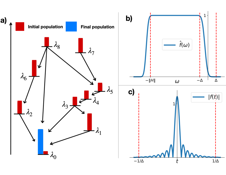
Figure 1: (a) Jablonski-like diagram illustrating the working principle of the ground state preparation algorithm, where high-energy components are progressively dissipated into lower-energy states, eventually reaching the ground state. The filter function in frequency (b) and time (c) domains, respectively.

To efficiently implement the jump operator $K_{a}$, it is not necessary to first diagonalize $H$, which would defeat the purpose. Instead, by expressing the $\hat{f}(\omega)$ as a filtering function in the time domain via the Fourier transform $f(s):=\frac{1}{2\pi}\int_{\mathbb{R}}\hat{f}(\omega)e^{-i\omega s}\mathrm{d}\omega$, we obtain

$$K_{a}=\int_{-\infty}^{\infty}f(s)e^{iHs}A_{a}e^{-iHs}\mathrm{d}s.$$ (3)

The filter function $f(s)$ is approximately supported on an interval of a size that is proportional to $\Delta^{-1}$ (Fig. 1 (c)). The integral can then be efficiently truncated and discretized for a quantum implementation of $K_{a}$. This transfers the quantum implementation of $K_{a}$ into the implementation of a linear combination of the Heisenberg evolution of the coupling operator $A_{a}$. We refer readers to [18] for the details of the quantum simulation of the Lindblad dynamics (1). We note that while the simulation algorithm proposed in [18] is designed for simulating a single jump operator using a single ancilla, when multiple jump operators are present, operator splitting can be applied to handle each jump operator separately. The overall simulation can still be carried out using a single ancilla. Many other Lindblad simulation algorithms [14, 40, 21] can also be employed to simulate this Lindblad dynamics, which can achieve a simulation cost that scales nearly linearly with the total evolution time. For the task here, the total evolution time can be characterized by the mixing time.

The standard definition of the mixing time respect to the trace distance $D(\rho,\sigma)=\frac{1}{2}\left\lVert\rho-\sigma\right\rVert_{1}$ is

$$\tau_{\operatorname{mix}}(\eta)=\min\left\{t\mid D(e^{\mathcal{L}t}\rho_{0},\sigma)\leq\eta,\;\;\forall\text{state }\rho_{0}\right\},$$ (4)

which is the minimal time for any initial state $\rho_{0}$ to reach the stationary state $\sigma$ within trace distance $\eta$. The trace distance, however, may be difficult to evaluate in practice. Alternative definitions of the mixing time, measured through physical observables such as energy and fidelity, can also be used; we will specify these when discussing relevant contexts. The rest of the manuscript focuses on characterizing the effectiveness of the dynamics (1) for ground state preparation measured by mixing times, which is the main quantity that determines the efficiency of this ground state preparation protocol.

III Quasi-free dissipative dynamics

Mapping spin systems to quasi-free dynamics—

The Hamiltonian of a 1D translationally invariant Transverse Field Ising Model (TFIM) with open boundary conditions is

$$H=-g\sum_{i=1}^{N}Z_{i}-J\sum_{i=1}^{N-1}X_{i}X_{i+1}.$$ (5)

Using the Jordan-Wigner transformation, the Hamiltonian can be written as a quadratic Majorana operator with $2N$ modes (Appendix B)

$$H=2iJ\sum_{j=1}^{N-1}w_{j+N}w_{j+1}+2ig\sum_{j=1}^{N}w_{j}w_{j+N}.$$ (6)

We choose the coupling operators to be Pauli matrices $X_{1}$ and $Y_{1}$ on the boundary of the chain, which are linear in the Majorana operators: $X_{1}=\sqrt{2}w_{1},Y_{1}=\sqrt{2}w_{1+N}$. By Thouless’s theorem, the Heisenberg evolution of a single Majorana operator under a quadratic Hamiltonian is still linear in Majorana operators. Therefore the jump operator in Eq. 3 can be expressed as

$$K_{a}=\sum_{j=1}^{2N}\zeta_{ja}w_{j},\quad A_{a}\in\{X_{1},Y_{1}\},$$ (7)

for some coefficients $\zeta_{ja}\in\mathbb{C}$.

We plot the heat map of the coupling operator $X_{1}$ in the computational basis, and the corresponding jump operator $K_{X_{1}}$ in the energy basis in Fig. 2. We find that although $X_{1}$ is very sparse in the computational basis, $K_{X_{1}}$ has significantly many more nonzero elements in the energy basis enabling transitions from high energy components to low energy ones. The filter function forbids transitions from low to high energy components. Therefore the jump operator is always an upper triangular matrix in the energy eigenbasis. Furthermore, the magnitude of the coefficients $|\zeta_{j}|^{2}+\left\lvert\zeta_{j+N}\right\rvert^{2}$ decays exponentially as $j$ increases ($1\leq j<N$), which implies that $K_{a}$ is quasi-local in Majorana operators (see Fig. 3).

Figure 2: (a). Matrix elements of a local Pauli operator $X_{1}$ in the computational basis. (b). Jump operator $K_{X_{1}}$ associated with coupling operator $X_{1}$ in the energy basis of the TFIM Hamiltonian with $N=8$ sites. The lower triangular part vanishes due to the filter function.

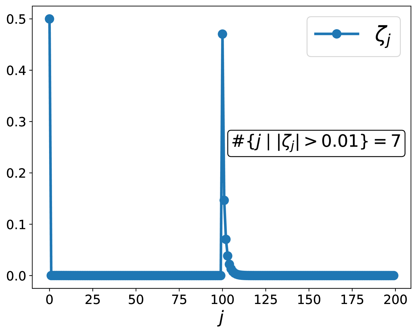
Figure 3: Coefficients of the jump operator under Majorana basis. $|\zeta_{j}|$ is calculated from (7) with $A_{a}=X_{1}$. System size is $N=100$.

Lindblad dynamics with a Hamiltonian term that is quadratic in Majorana operators, and jump operators linear in Majorana operators is called quasi-free. Using a vectorization process known as “third quantization” [52, 5], each term in the vectorized Lindbladian becomes quadratic in an enlarged set of Majorana operators. Physical observables of a quasi-free dynamics, such as the covariance matrix

$$\Gamma_{pq}=i\braket{w_{p}w_{q}}-\frac{i}{2}\delta_{pq},$$ (8)

form a closed set of equations, which involves only a matrix of size $2N\times 2N$ in time (Appendix B). This in turn can be used to evaluate other physical quantities such as the energy. Specifically, for a Hamiltonian quadratic in Majorana operators, $H=\sum_{p,q=1}^{2N}h_{pq}w_{p}w_{q}$, where $h$ is a Hermitian and purely imaginary (and thus traceless) coefficient matrix, the energy is given by

$$E=\sum_{pq}h_{pq}\braket{w_{p}w_{q}}=i\mathrm{Tr}[h^{T}\Gamma].$$ (9)

For quasi-free systems with Gaussian initial states, higher order covariance matrices are determined by the covariance matrix $\Gamma$ according to Wick’s theorem [61].

TFIM with boundary dissipation—

Similar to the derivation in Appendix B, if we choose the Pauli operators $X_{N},Y_{N}$ on the other end of the boundary, the resulting Lindblad dynamics is also quasi-free. Hence we choose $\{X_{1},Y_{1},X_{N},Y_{N}\}$ to be the coupling operators, and construct the corresponding jump operators according to Eq. 3.

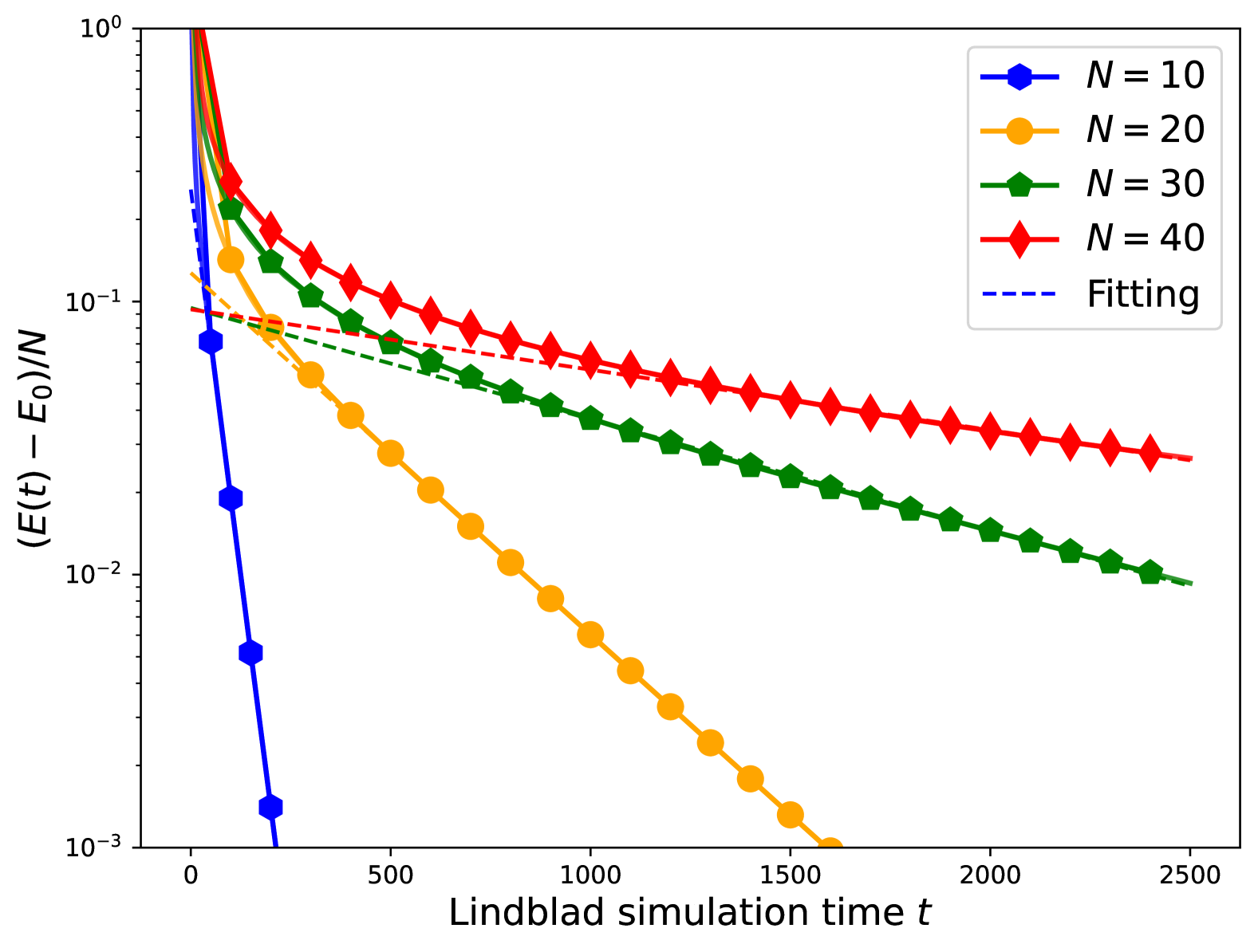
(a) Energy decay vs time $t$

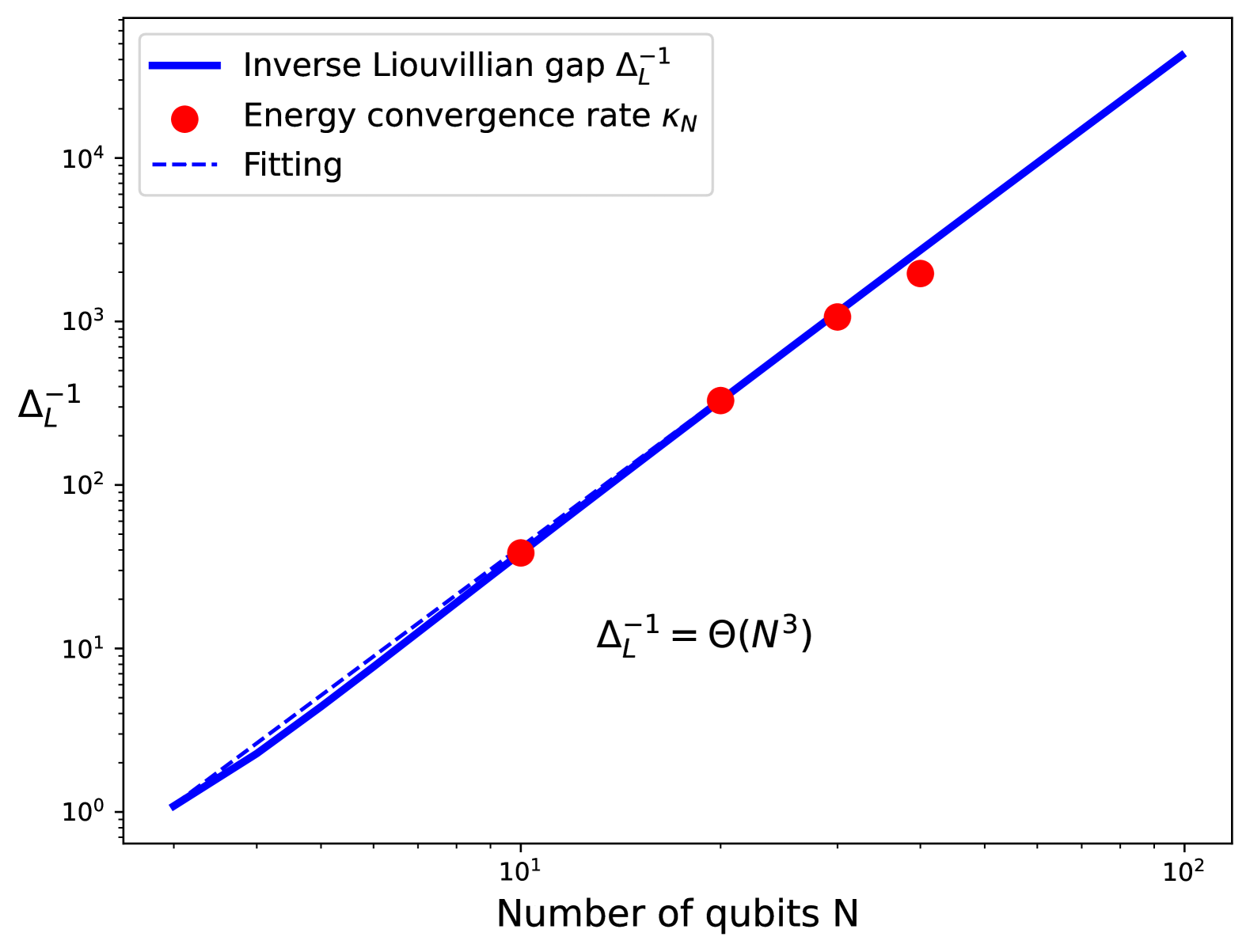
(b) $\Delta^{-1}_{\mathcal{L}}$ vs system size $N$

Figure 4: Numerical results of 1D TFIM (5) with $J=1,g=1.5$, using $\{A_{a}\}=\{X_{1},Y_{1},X_{N},Y_{N}\}$ as coupling operators. (a) Convergence of energy starting from the maximally mixed state. The dashed lines are exponential fits of the asymptotic behaviour of energy decay, meaning $(E(t)-E(0))/N=\Theta(\exp(-\kappa_{N}t))$ for constants $\kappa_{N}$ when $t$ is sufficiently large. (b) The scaling of the inverse of the Liouvillian gap $\Delta^{-1}_{\mathcal{L}}$ with respect to the system size $N$. Red points are the energy convergence rate $\kappa_{N}$ calculated from fitting the data in (a).

Using the covariance matrix $\Gamma(t)$, we can evaluate the energy $E(t)$ via Eq. 9. We note that the convergence of the many-body density matrix cannot always be inferred from the covariance matrix $\Gamma(t)$. As a surrogate, in this section, we characterize the mixing time based on the convergence of the energy, normalized by the system size $N$. Specifically, we define the mixing time measured by the energy:

$$\tau^{E}_{\operatorname{mix}}(\eta;\rho_{0})=\min\left\{t\mid\left\lvert E(t)-E_{0}\right\rvert/N\leq\eta\right\},$$ (10)

starting from the maximally mixed initial state $\rho_{0}=\mathbb{I}/2^{N}$. Since the convergence in trace distance provides an upper bound of the convergence of any bounded physical observables, we expect that the scaling of the mixing time with respect to the system size $N$ measured by $\tau^{E}$ closely aligns with that measured by the trace distance in Eq. 4. This will be theoretically verified in Section IV.

Fig. 4a demonstrates the energy decay of the boundary-dissipated TFIM under Lindbladian dynamics. The initial state is set to be the maximally mixed state. Numerical simulations show that the energy rapidly converges towards the ground state energy initially, and then enters an asymptotic exponentially decaying regime $\propto e^{-\Delta_{\mathcal{L}}t}$. The convergence rate $\Delta_{\mathcal{L}}$ is the gap of the Lindbladian (also called the Liouvillian gap). We may extract $\Delta_{\mathcal{L}}$ using an exponential fit of the dynamics, and can also directly compute $\Delta_{\mathcal{L}}$ by means of the rapidity spectrum for quasi-free systems [53]. In Fig. 4b, we show how the Liouvillian gap scales with the system size. The estimates for $\Delta_{\mathcal{L}}$ from the slopes in Fig. 4a yield excellent agreement with the rapidity spectrum calculations. Using a log-log scaling for the axes, we find that $\Delta_{\mathcal{L}}=\Theta(N^{-3})$. Therefore for fixed accuracy $\eta$, the mixing time $\tau^{E}_{\operatorname{mix}}=\Theta(N^{3})$. Note that this is a different statement from claiming that the mixing time in trace distance scales as $\Theta(N^{3})$.

Importance of the coherent term—

In the case of boundary dissipation with coupling operators $X_{1},X_{N},Y_{1},Y_{N}$, the coherent term $-i[H,\cdot]$ plays a critical role for the system to converge to the ground state, as illustrated in Fig. 5. Physically, since the jump operator is localized near the boundary, dissipation primarily occurs there. The coherent term induces an energy flux from the bulk to the boundary, which effectively reduces the energy.

Mathematically, without the coherent term, the Lindblad dynamics lacks a unique fixed point. The role of the coherent term is to lift this large degeneracy, and place eigenvalues on the imaginary axis. The dissipative term then slightly perturbs these eigenvalues away from the imaginary axis, creating a spectral gap that leads to convergence. This will be rigorously justified in Section IV.

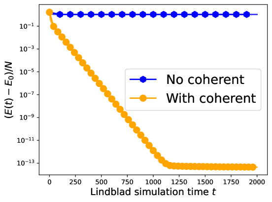
Figure 5: Convergence of energy in TFIM using $\{X_{1},X_{N},Y_{1},Y_{N}\}$ as coupling operators, with and without the coherent term $-i[H,\cdot]$ in the Lindbladian.

Cluster state Hamiltonian with boundary dissipation—

The 1D cluster state Hamiltonian on $N$ sites takes the form

$$H=-J\sum_{j=1}^{N-2}X_{j}Z_{j+1}X_{j+2}-h_{1}\sum_{j=1}^{N}Z_{j}.$$ (11)

This system plays a role in measurement-based quantum computing [7, 55], and exhibits an interesting symmetry protected topological (SPT) phase, with a four-fold degenerate ground state in the thermodynamic limit [59, 15]. The field strength $h_{1}/J$ drives a phase transition between a simple paramagnetic phase and the SPT phase. Using the Jordan-Wigner transformation, the Hamiltonian can be expressed as a quadratic Majorana operator

$$H=2iJ\sum_{j=1}^{N-1}w_{j+N}w_{j+2}+2ih_{1}\sum_{j=1}^{N}w_{j}w_{j+N},$$ (12)

which is similar to a Kitaev chain Hamiltonian with next-nearest-neighbor (NNN) couplings. The string order parameter (SOP) is a non-local order parameter which can be used to distinguish between the SPT phase and the paramagnetic phase. It is defined as

$$S_{ab} =X_{a}Z_{a+1}Z_{a+3}\ldots Z_{b-3}Z_{b-1}X_{b}$$ (13)

$$=2^{\frac{b-a}{2}}\prod_{i=1}^{\frac{b-a}{2}}w_{a+2i}\prod_{i=0}^{\frac{b-a}{2}-1}w_{a+N+2i},$$

where $a,b$ are arbitrary starting and ending points in the bulk with $b-a$ being an even number. The SOP can be computed using Wick’s theorem [61]

$$\left\langle S_{a,b}\right\rangle=2^{\frac{b-a}{2}}\left\langle\prod_{i=1}^{\frac{b-a}{2}}w_{a+2i}\prod_{i=0}^{\frac{b-a}{2}-1}w_{a+n+2i}\right\rangle=\operatorname{Pf}\left(2\Gamma_{\left.\right|\{q\}}\right),$$ (14)

where $\Gamma_{\left.\right|\{q\}}$ is the covariance matrix restricted to the indices $\{q\}=\{a+2i,a+n+2(i-1)|i=1,\ldots b-a\}$ and $\operatorname{Pf}$ denotes the Pfaffian.

We choose the coupling operators to be two single Pauli operators on two ends of the boundary $A_{1}=Y_{1},A_{2}=Y_{N}$. The corresponding jump operators are linear in Majorana operators, and the dissipative dynamics is thus quasi-free. The presence of zero energy edge modes in the SPT phase of the system lead to nearly degenerate ground states with energy gaps closing exponentially rapidly as the system size increases. However, the closing of the energy gap is entirely due to the presence of the edge modes which is irrelevant for bulk properties such as the SOP. Therefore we may define an effective gap, denoted by $\Delta_{\mathcal{L},\rm{eff}}$, by excluding the eigenvalues in the Liouvillian exponentially clustering near $0$, and choose the parameters in the filter function $\hat{f}(\omega)$ based on this effective gap. When choosing effective gap $\Delta_{f}=0.1$ in $f$, the resulting dissipative dynamics converges to a statistical mixture of the nearly degenerate states with the same SOP value in the thermodynamic limit (Fig. 6). The SOP is evaluated by setting $a,b$ to be the two ends of the chain. We find again that boundary dissipation alone is sufficient to drive the system from a paramagnetic phase towards SPT phase.

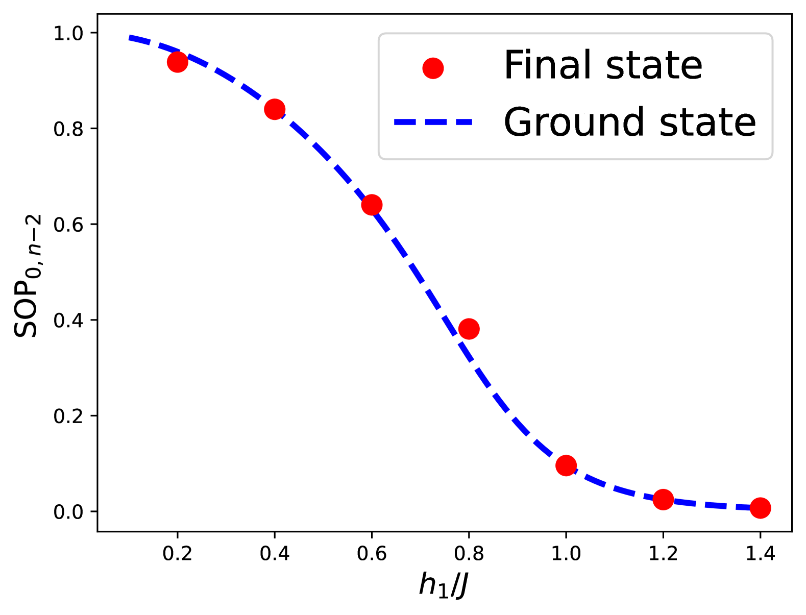
(a) SOP with respect to $h_{1}/J$.

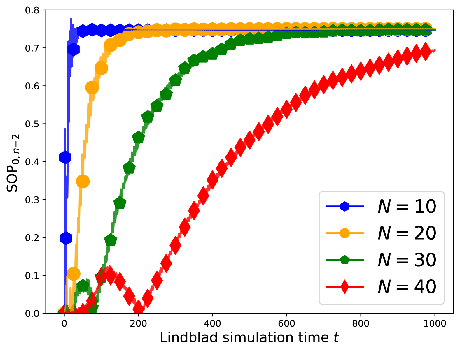
(b) Convergence of SOP as $N$ increases.

Figure 6: Evolution of the string order parameter (SOP) for the cluster state Hamiltonian  (11) with boundary dissipation. The system size is $N=20$. (a) SOP comparison between the ground state (blue dashed line) and the final state at $T=1500$ (red points). The final state accurately captures the quantum phase transition from the paramagnetic phase to the SPT phase. (b) Evolution of the SOP for several system sizes with $h_{1}/J=0.5$, whose ground state is in the SPT phase. The initial state is the all-spin-down state, which is in the paramagnetic phase with $\text{SOP}=0$. The dissipative evolution consistently drives the system from the paramagnetic phase into the SPT phase.

Next, we examine how the convergence rate of Lindbladian dynamics scales with the system size. As in the study of the SOP, we set the coupling operators to be single Pauli $Y$ operators at the two ends of the system ($A_{1}=Y_{1}$ and $A_{2}=Y_{N}$) and fix $\Delta_{f}=0.1$ for all $N$. In Fig. 7(a), we plot the energy decay of the SPT system with $h_{1}/J=0.4$. For $N=20,30,40$, similar to the 1D TFIM case, the energy rapidly approaches the ground state energy at early times before entering an asymptotic regime characterized by exponential decay. We note that for $N=10$ an energy plateau appears. This is because the Hamiltonian in Eq. 11 has a four-fold degenerate ground state in the thermodynamic limit. For small system sizes, there is still a small energy gap between these nearly degenerate states, which is smaller than our chosen $\Delta_{f}$. Reducing $\Delta_{f}$ would further lower the plateau. In Fig. 7(b), we illustrate how the effective Liouvillian gap scales with system size. For various values of $h_{1}/J$, we consistently observe that the inverse effective gap scales as $\Delta_{\mathcal{L},\rm{eff}}^{-1}=\Theta(N^{3})$. Consequently, to achieve a fixed accuracy $\eta$, the mixing time scales as $\tau^{E}_{\operatorname{mix}}=\mathcal{O}(N^{3})$.

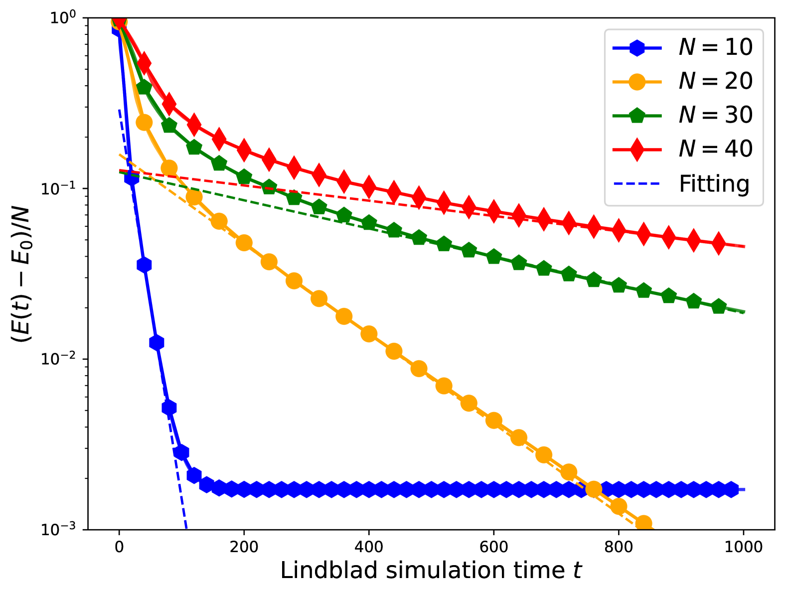
(a) Energy decay vs time $t$

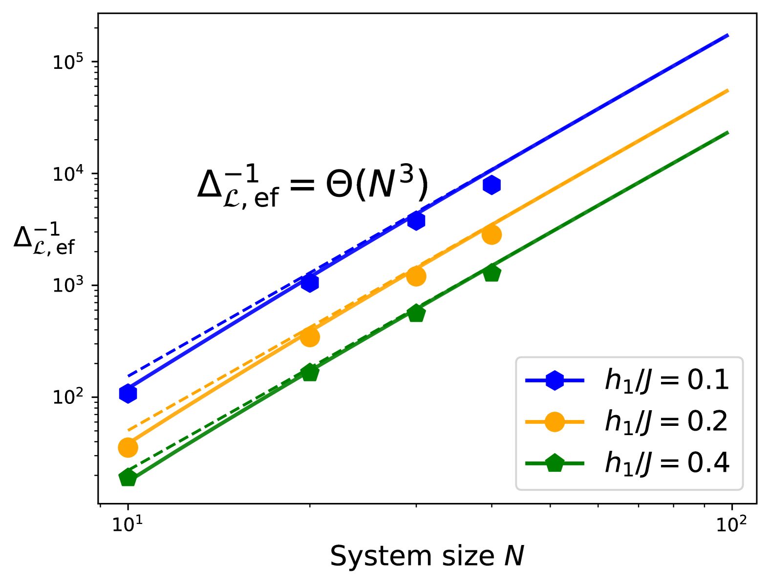
(b) $\Delta_{\mathcal{L},\rm{eff}}^{-1}$ vs system size $N$

Figure 7: Numerical results for the cluster state Hamiltonian (11) with boundary dissipation. (a) Convergence of energy starting from the maximally mixed state. Here, we use boundary dissipation and set $\Delta_{f}=0.1$, $h_{1}/J=0.4$. The dashed lines are exponential fits of the asymptotic behaviour of energy decay before hitting the energy plateau caused by the exponentially decaying edge modes. (b) The scaling of the inverse of the effective Liouvillian gap $\Delta^{-1}_{\mathcal{L},\rm{eff}}$ with respect to the system size $N$ with different $h_{1}/J$. Points are the fitting energy convergence rate $\kappa_{N}$ calculated from dynamics simulation.

IV Explicit bound of mixing time in trace distance for quasi-free systems

In order to characterize convergence rate of Lindblad dynamics, one standard approach is to evaluate the Liouvillian gap. When the dissipative dynamics satisfies the quantum detailed balance condition (DBC), the Lindbladian may be transformed into a Hamiltonian under a similarity transformation, and the Liouvillian gap can be bounded using techniques for bounding spectral gaps for quantum many-body Hamiltonians [56, 66]. This strategy, however, cannot be applied to Lindblad dynamics with a coherent term which breaks the DBC.

A more general formulation for bounding the spectral gap may be captured by the hypocoercivity theory, which was originally formulated in the context of classical kinetic theory [73] and has recently been applied in the context of open quantum systems described by Lindblad equations [24]. However, the formulation in [24] can only be used to prove the existence of an spectral gap. For quasi-free dynamics, the spectral gap can also be derived explicitly from the rapidity spectrum [53] related to the equation of motion for the covariance matrix.

Even with spectral gap estimates, the problem remains how to bound convergence of the density matrix in trace distance. This is because spectral gap estimates only imply convergence in $\chi^{2}$-distance [62], and the conversion from convergence in $\chi^{2}$-distance to the trace distance involves a factor that blows up exponentially as temperature decreases, making it inapplicable for ground state preparation when the temperature is zero. A special technique called hypercontractivity can be applied to quasi-free quantum groups [64] but also requires the stationary state to be invertible.

Below we provide a general theory giving an explicit bound on convergence in trace distance to the singular ground state $\sigma$ for general quasi-free dynamics. When applied to the TFIM model, we find that the convergence rate estimate is also sharp, in the sense that the mixing time in our analysis does not involve an additional multiplicative factor arising from the conversion from the $\chi^{2}$-distance to the trace distance. This multiplication factor can grow polynomially in the system size in the finite temperature setting, and becomes unbounded in the zero temperature setting in the worst case. The specific form of the jump operator constructed in [18] turns out to be a key component. In other words, our analysis does not apply to arbitrary quasi-free dynamics.

We provide some high-level ideas of our strategy below. To prove the convergence in trace distance, we use the Fuchs–van de Graaf inequality

$$D(\rho,\sigma)\leq\sqrt{1-F(\rho,\sigma)^{2}},$$ (15)

where $F(\rho,\sigma)^{2}=\operatorname{Tr}\left[\sqrt{\rho^{\frac{1}{2}}\sigma\rho^{\frac{1}{2}}}\right]^{2}$ is the square of the fidelity. The ground state of any Hamiltonian that is quadratic in Majorana operators can be written as a quasi-vacuum state $\sigma=|\mathrm{vac}\rangle\!\langle\mathrm{vac}|$, with

$$b_{k}\left|\mathrm{vac}\right\rangle=0,\quad k=1,\ldots,2N,$$ (16)

for a properly defined set of fermionic annihilation operators $\{b_{k}\}$ (Appendix B). Let $\hat{N}=\sum_{k}b_{k}^{{\dagger}}b_{k}$ be the total number operator. Note that all states other than $\left|\mathrm{vac}\right\rangle$ has at least one particle. This gives the inequality

$$1-\braket{\mathrm{vac}|\rho|\mathrm{vac}}=\mathrm{Tr}[\rho(I-|\mathrm{vac}\rangle\!\langle\mathrm{vac}|)]\leq\mathrm{Tr}[\rho\hat{N}].$$ (17)

However, it turns out that the number operator does not provide a useful bound on convergence. Our key innovation is to find a positive definite observable $O$, which is equivalent to the number operator in the sense that there exist constants $C_{1},C_{2}$ such that $C_{1}\hat{N}\preceq O\preceq C_{2}\hat{N}$. Then, for a proper choice of $O$, we prove the sharp exponential convergence

$$\mathrm{Tr}[O\rho(t)]\leq\mathrm{Tr}[O\rho(0)]e^{-2\Delta t}.$$ (18)

This relation, after plugging back into (15), gives the desired exponential convergence with the explicit convergence rate $\Delta$. The construction of $O$ is related to concepts in the hypocoercivity theory, and $\mathrm{Tr}[O\rho]$ may be viewed as a Lyapunov function of the Lindblad dynamics.

We find that the convergence rate $\Delta$, as well as the constants $C_{1},C_{2}$, are determined by a non-Hermitian quadratic Hamiltonian

$$H_{\rm nh}=iH-\frac{1}{2}\sum_{a}K_{a}^{{\dagger}}K_{a}=\sum_{p,q=1}^{2N}(h_{\mathrm{nh}})_{pq}w_{p}w_{q},$$ (19)

where $h_{\mathrm{nh}}$ is a non-Hermitian matrix in general. Assume $h_{\mathrm{nh}}$ is diagonalizable as $h_{\mathrm{nh}}=VDV^{-1}$, then $\Delta$ is given by the non-Hermitian gap $-\max_{i}\operatorname{Re}D_{ii}$.

In fact, for an arbitrary observable $X$, the adjoint of the Lindbladian $\mathcal{L}^{{\dagger}}$ can be expressed as

$$\mathcal{L}^{{\dagger}}(X)=H_{\rm nh}X-XH^{{\dagger}}_{\rm nh}+\sum_{a}K_{a}^{{\dagger}}XK_{a}.$$ (20)

Our result demonstrates that the Liouvillian gap is entirely determined by the non-Hermitian Hamiltonian $H_{\rm nh}$ and is independent of the complete positive term $\sum_{a}K_{a}^{{\dagger}}XK_{a}$, commonly referred to as the transition part. This is somewhat counterintuitive, as the transition part is precisely what facilitates the transition to the ground state!

We now present our main theorem for quasi-free systems in Theorem 21, with the proof provided in Appendix C.

Theorem 1.

Let $H$ be a gapped quadratic Majorana Hamiltonian with $2N$ modes, $\{A_{a}\}$ be a set of coupling operators that are linear in Majorana operators, and $K_{a}$ be the corresponding jump operators defined via Eq. 3. We consider the non-Hermitian Hamiltonian in Eq. 19, assume the coefficient matrix $h_{\mathrm{nh}}$ is diagonalizable with $h_{\mathrm{nh}}=VDV^{-1}$, and define the non-Hermitian gap $\Delta=-\max_{i}\operatorname{Re}D_{ii}$. We denote the condition number of $V$ by $\kappa(V)$.

If $\Delta>0,\kappa(V)<\infty$, then starting from any initial state $\rho_{0}$, the Lindblad dynamics (1) converges exponentially in trace distance to the quasi-vacuum state $\sigma=|\mathrm{vac}\rangle\!\langle\mathrm{vac}|$ with

$$D(\rho(t),\sigma)\leq\kappa(V)\sqrt{2N}e^{-\Delta t}.$$ (21)

An immediate result from Theorem 21 is that the mixing time defined in the trace distance in Eq. 4 scales as

$$t_{\mathrm{mix}}(\eta)\leq\Delta^{-1}\log\left(\frac{\kappa(V)\sqrt{2N}}{\eta}\right).$$ (22)

Therefore as long as $\kappa(V)=\operatorname{poly}(N)$, the scaling of the mixing time is determined by the scaling of the non-Hermitian gap $\Delta$ with respect to $N$, up to a logarithmic factor.

Application to TFIM with boundary dissipation—

The $\mathcal{O}(N^{3})$ scaling for boundary-dissipated 1D translationally invariant TFIM has been observed in previous studies [75], where the jump operator is strictly applied to a single site on the boundary. Their proof maps the problem to a non-Hermitian Su-Schrieffer-Heeger (SSH) model, which enables an analytic computation of the rapidity spectrum. In contrast, our jump operators ${K_{a}}$ are quasi-local, rendering this technique inapplicable. Instead, we leverage the stronger result in Theorem 21 to directly bound the convergence in trace distance.

For simplicity we only consider the case when the coupling operators are $X_{1},Y_{1}$ on one end of the boundary. First, following the proof of Theorem 21 in Appendix C, the jump operators take the form

$$K_{X_{1}} =\int f(s)e^{iHs}X_{1}e^{-iHs}\,\mathrm{d}s=\sum_{k}\varphi_{k1}b_{k},$$ (23)

$$K_{Y_{1}} =\int f(s)e^{iHs}Y_{1}e^{-iHs}\,\mathrm{d}s=\sum_{k}\psi_{k1}b_{k},$$

for some coefficient vectors $\{\varphi_{k1}\},\{\psi_{k1}\}$, where the ground state is a quasi-vaccum state satisfying $b_{k}\left|\mathrm{vac}\right\rangle=0$. Let $\Lambda$ be a diagonal matrix encoding the eigenvalues of the TFIM Hamiltonian $H$, then the non-Hermitian Hamiltonian in Eq. 19 can be written as

$$H_{\rm nh}=\mathbf{b}^{{\dagger}}h_{\mathrm{nh}}^{f}\mathbf{b},\quad h^{f}_{\mathrm{nh}}=i\Lambda-\frac{1}{2}\varphi\varphi^{{\dagger}}-\frac{1}{2}\psi\psi^{{\dagger}}.$$ (24)

The crucial role of the coherent term in convergence is now evident. Without the coherent $i\Lambda$, $h^{f}_{\mathrm{nh}}$ is merely a rank-2 matrix, resulting in a large kernel for $H_{\rm nh}$ and the non-Hermitian gap $\Delta=0$. When the coherent term is present, the jump operators can shift the imaginary eigenvalues $i\Lambda$ away from the real axis, opening a positive spectral gap.

Using first-order perturbation theory, we estimate the spectral gap as $\Delta=\Theta(N^{-3})$. The cubic scaling is mainly due to long-wavelength modes, whose magnitude scales as $\mathcal{O}(N^{-1.5})$ near the boundary. The square of this magnitude determines the spectral gap from the real axis, perturbing the eigenvalues from the imaginary axis by an amount proportional to $N^{-3}$.

Furthermore, $\kappa(V)=\mathcal{O}(1)$, which gives the mixing time scaling as $\mathcal{O}(N^{3}\log N)$. We provide the details in Appendix D. We expect the analysis for the cluster state Hamiltonian may be derived with a similar argument and is omitted here.

V Matrix product operator based formalism for classical simulation of Lindblad dynamics

If the Lindblad dynamics is not quasi-free, we need to simulate the dynamics in Eq. 1 directly to estimate the mixing time. For system sizes beyond the reach of exact diagonalization (ED), we propose an algorithm that constructs the jump operators and propagates the Lindblad dynamics using a matrix product operator (MPO) formulation. Recall that an MPO on an $N$-site system (each site of local dimension $d$) with bond dimension $D$ can be written as

$$M=\sum_{s_{1},s_{1}^{\prime},\ldots,s_{N},s_{N}^{\prime}=1}^{d} \Bigl{(}M_{1}^{s_{1},s_{1}^{\prime}}\cdots M_{N}^{s_{N},s_{N}^{\prime}}\Bigr{)}\cdot$$ (25)

$$\left|s_{1},\ldots,s_{N}\right\rangle\!\left\langle s_{1}^{\prime},\ldots,s_{N}^{\prime}\right|,$$

where $M_{1}^{s_{1},s_{1}^{\prime}}\cdots M_{N}^{s_{N},s_{N}^{\prime}}$ defines the corresponding matrix product, with $M_{1}^{s_{1},s_{1}^{\prime}}\in\mathbb{C}^{1\times D},M_{N}^{s_{N},s_{N}^{\prime}}\in\mathbb{C}^{D\times 1}$, and $M_{i}^{s_{i},s_{i}^{\prime}}\in\mathbb{C}^{D\times D}$ for $2\leq i\leq N-1$. The cost of storing the matrix products is $\mathcal{O}(d^{2}D^{2}N)$, which scales linearly with the system size $N$.

To construct the jump operators $K_{a}$, we start by representing both the coupling operators $A_{a}$ and the Hamiltonian $H$ as MPOs. We then compute the Heisenberg evolution $e^{iHs}A_{a}e^{-iHs}$ using the time-evolving block-decimation (TEBD) algorithm [71, 69]. Next, we approximate the integral in Eq. 3 by a quadrature rule,

$$K_{a}\approx\sum_{i}p_{i}\,f(s_{i})\,e^{iHs_{i}}A_{a}\,e^{-iHs_{i}},$$ (26)

and compress the resulting sum to maintain a manageable bond dimension. This yields the MPO representation of the jump operator $K_{a}$ (see Fig. 8 for an illustration).

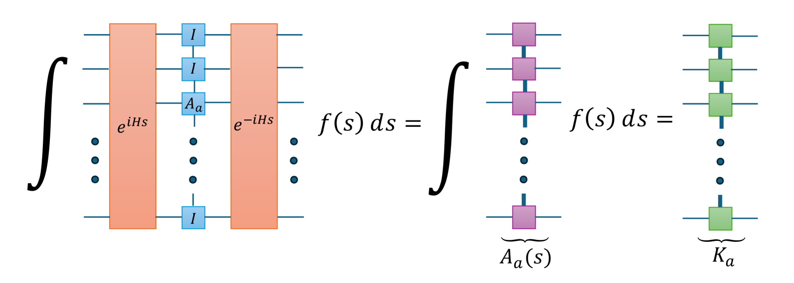
Figure 8: Tensor network representation of the jump operator $K_{a}$ in the MPO form associated from a local coupling operator $A_{a}$. First, the MPO representation of the operator $e^{iHs_{j}}A_{a}e^{-iHs_{j}}$ is constructed for a set of time steps $\{s_{j}\}$. Next, a weighted summation from discretizing the integral $\sum_{j}p_{j}f(s_{j})e^{iHs_{j}}A_{a}e^{-iHs_{j}}$ is performed to combine these operators. Finally, the resulting MPO is compressed to reduce the bond dimension, yielding an efficient representation of $K_{a}$.

In practice, since $A_{a}$ is an operator rather than a state, the TEBD algorithm is implemented by vectorizing $A_{a}$ into an MPS (often referred to as the Choi isomorphism). Concretely, we reshape each site’s row and column indices into a single combined index of dimension $d^{2}$, as illustrated in Fig. 9:

$$\left|M\right\rangle_{\sharp}=\sum_{i_{1}=0}^{d^{2}-1}\cdots\sum_{i_{N}=0}^{d^{2}-1}c_{i_{1},\ldots,i_{N}}\,\left|i_{1}\right\rangle_{\sharp}\otimes\cdots\otimes\left|i_{N}\right\rangle_{\sharp}.$$ (27)

In a tensor network diagram, this corresponds to “gluing” the row and column indices together on each site. Converting back from an MPS to an MPO is achieved by splitting each combined index back into two separate indices. Under vectorization, the Heisenberg evolution can be written as

$$\left|\,e^{iHs}A_{a}\,e^{-iHs}\right\rangle_{\sharp}\;=\;e^{-i\,(I\otimes H^{T}\,-\,H\otimes I)\,s}\,\left|A_{a}\right\rangle_{\sharp},$$ (28)

so that the standard TEBD algorithm can be applied directly. To compute the jump operator $K_{a}$, we proceed as follows: (i) convert $A_{a}$ from its MPO form into an MPS using the Choi isomorphism, (ii) apply TEBD to evolve the vectorized operator over time, and (iii) perform a summation over the discrete time steps, followed by bond dimension compression. The resulting MPS is then converted back into an MPO, yielding $K_{a}$.

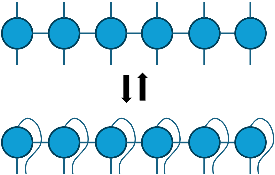
Figure 9: Illustration of vectorizing an MPO into an MPS using the Choi isomorphism and then converting it back. Each pair of local site indices in the MPO is reshaped into a single combined index, allowing standard MPS techniques, such as TEBD, to be applied. The reverse process restores the original MPO from the MPS by reshaping the combined indices back into pairs.

Once each jump operator is expressed as an MPO, and given that $\rho(t)$ is also stored as an MPO, we need to evaluate the right-hand side of Eq. 1, i.e., $\mathcal{L}(\rho(t))$. This illustrated using tensor network diagrams in Fig. 10. However, direct multiplication and addition of MPOs tend increases the bond dimension quickly. For example, in the absence of a compression step, multiplying two MPOs with bond dimension $D$ results in an MPO with bond dimension $D^{2}$, while adding two MPOs yields an MPO with bond dimension $2D$. If we choose $\{A_{a}\}$ to be the set of all Pauli matrices, and assume every operator in the Lindbladian has bond dimension $D$, the bond dimension of the MPO representation for $\mathcal{L}(\rho)$ would become $\mathcal{O}(ND^{3})$.

Forming such an MPO and then compressing it would have an onerous cost of $\mathcal{O}(D^{9})$. Instead, we directly fit an MPO of bond dimension $D$ to the uncontracted sum of triple MPO products as depicted in Fig. 10, adapting the method of [68]. This only requires computing the overlap of the ansatz with these terms (see Appendix E). The initial guess is chosen as the “zip-up” compression [60] of the first term. Both this and the subsequent fitting iterations have a cost of $\mathcal{O}(D^{5})$.

After obtaining the compressed MPO representation of $\mathcal{L}(\rho)$, we may employ any suitable numerical integrator to propagate $\rho(t)$ forward in time. For large systems, each evaluation of $\mathcal{L}(\rho)$ is expensive, so it is beneficial to minimize the number of function evaluations. For bulk dissipation, the cost of evaluating $\mathcal{L}(\rho)$ is large, but the mixing time can be very short. Therefore we adopt a simple forward-Euler method. For boundary dissipation, the mixing time can be much longer, and there we employ a more accurate 4th-order Runge-Kutta method instead. More advanced solvers can be explored in future studies to improve the accuracy or efficiency.

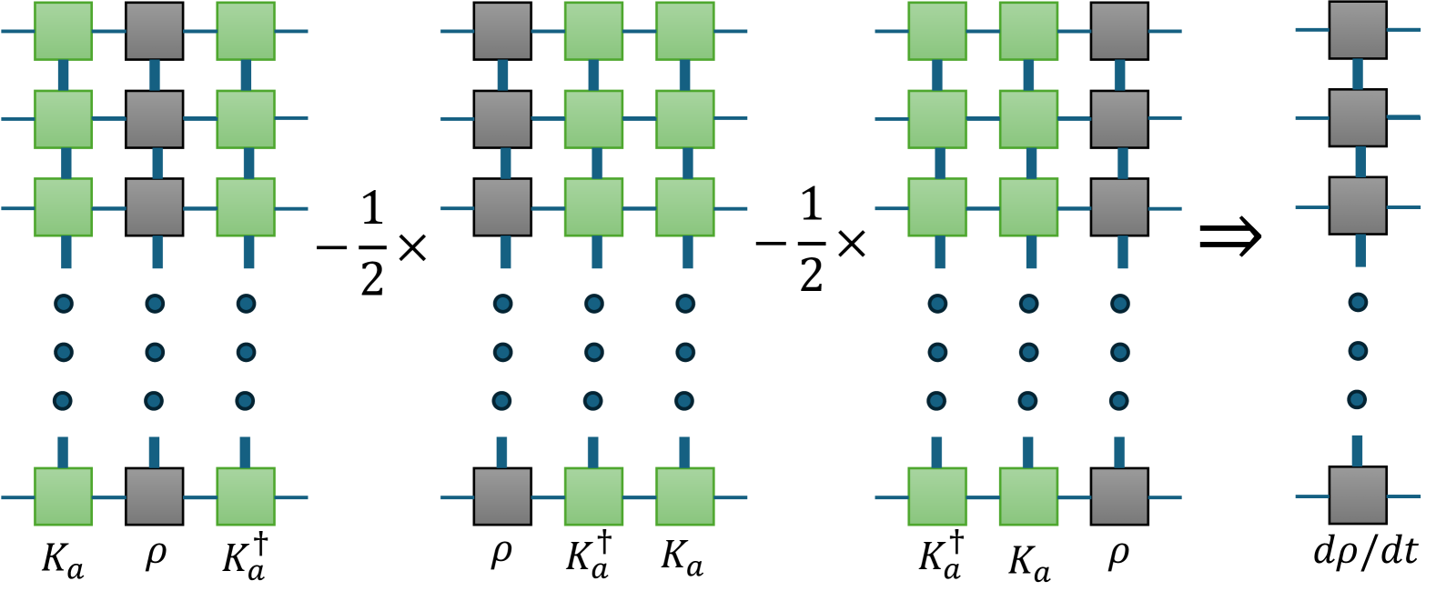
Figure 10: Illustration of the tensor network computation associated with a single jump operator $K_{a}$ in $\mathcal{L}(\rho)$.

VI Numerical results of tensor network based simulation

Rapid mixing of 1D gapped local Hamiltonians

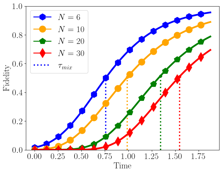
Figure 11: The mixing time, $\tau^{F}_{\mathrm{mix}}$, as defined in (30). During the Lindbladian dynamics, the fidelity increases steadily and eventually converges to one. However, the convergence speed decreases as the system size increases.

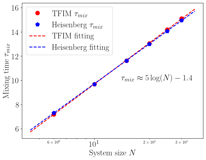
Figure 12: Scaling of the mixing time for TFIM (red) and the Heisenberg model in a magnetic field (blue) under bulk dissipation, shown as a function of system size. The results indicate a logarithmic scaling, consistent with $\tau^{F}_{\mathrm{mix}}=\Theta(\log(N))$.

As an application of our tensor network based algorithm, we prepare the ground state of two examples of 1D gapped, non-commuting local Hamiltonians using bulk dissipation, i.e., the coupling operators are chosen to be the Pauli operators $\{X_{i},Y_{i},Z_{i}\}$ on all sites. The first one is the same TFIM example in Eq. 5 with $J=1,g=1.5$. The second example, which cannot be transformed into a free fermionic system, is an anisotropic Heisenberg model in a magnetic field, described by the Hamiltonian

$$H=-J\sum_{i=1}^{N-1}X_{i}X_{i+1}-\xi\sum_{i=1}^{N-1}(Y_{i}Y_{i+1}+Z_{i}Z_{i+1})-g\sum_{i=1}^{N}Z_{i}.$$ (29)

Here we choose the parameters $g=1.5,J=1$ and $\xi=0.1$. We simulate their Lindblad dynamics for system sizes up to $N=30$. The initial state is chosen to be the maximally mixed state. The bond dimension $D$ of the MPO representation for both the jump operators and the density matrix is set to 50. We validate this choice of the bond dimension in Appendix E.

In this section, we measure the mixing time with respect to the fidelity

$$\tau^{F}_{\operatorname{mix}}(\eta;\rho_{0})=\min\left\{t\mid\langle\psi|\rho_{t}|\psi\rangle\geq 1-\eta\right\}.$$ (30)

Unless otherwise mentioned, we choose $\eta=\frac{1}{2}$ and start from the maximally mixed state $\rho_{0}=\mathbb{I}/2^{N}$. The results in Fig. 12 demonstrate that the mixing times in both cases scale logarithmically with the system size; this scaling is often referred to as “rapid mixing” [4, 35].

TFIM with random transverse field—

Now consider the 1D transverse field Ising model but with a random transverse field

$$H=-\sum_{i=1}^{N}g_{i}Z_{i}-J\sum_{i=1}^{N-1}X_{i}X_{i+1},$$ (31)

where the strength of the transverse field $g_{i}\sim\mathcal{N}(2,\sigma^{2})$ and $\sigma^{2}$ is the variance parameter. Due to Anderson localization, for any $\sigma>0$, the eigenfunctions of $H$ are exponentially localized in space. This means that choosing single Pauli operators on the boundary produces a large number of inaccessible “dark modes” (i.e., $\left\langle\psi_{i}|A_{a}|\psi_{j}\right\rangle\approx 0$), which means that boundary dissipation alone may lead to an exponentially long mixing time, or fail to converge to the ground state altogether. Nonetheless, the bulk dissipation is not subject to this failure mechanism due to Anderson localization. We choose the set of coupling operators $\{A_{a}\}$ to be all Pauli operators $\{X_{i},Y_{i},Z_{i}\}_{i=1}^{N}$. We simulate the resulting Lindblad dynamics using the tensor network methods for system sizes up to $N=16$. Fig. 13 illustrates the scaling behavior of the mixing time as a function of the system size $N$. Our results indicate a logarithmic scaling of the mixing time, suggesting that ground state preparation can be efficiently achieved using bulk dissipation.

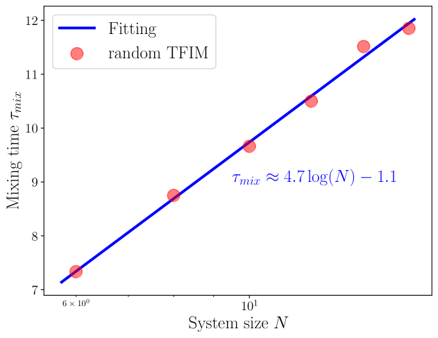
Figure 13: The scaling of the mixing time of random TFIM under bulk dissipation, i.e. we use $3N$ separate jump operators with the set of all Pauli operators on each sites as coupling operators $\{X,Y,Z\}^{N}$. The Hamiltonian parameters are set to $J=1,\sigma^{2}=0.5$. We observe a logarithmic scaling of the mixing time.

Non-integrable cluster state Hamiltonian—

We now consider the following generalization of the cluster state Hamiltonian

$$H=-\sum_{i=1}^{N-2}X_{i}Z_{i+1}X_{i+2}-h_{1}\sum_{i=1}^{N}Z_{i}-h_{2}\sum_{i=1}^{N-1}Z_{i}Z_{i+1}.$$ (32)

When $h_{2}\neq 0$, the Hamiltonian cannot be transformed into a free fermionic system. Nonetheless, the ground state can still exhibit the SPT phase characterized by a nonzero string order parameter (SOP).

As an illustration, we choose the coupling operators to be single Pauli operators on the boundary $A_{1}=Y_{1},A_{2}=Y_{n}$. The parameters for $h_{1}=0.4,h_{2}=-0.4$ are set so that the ground state is in the SPT phase. We simulate the Lindblad dynamics starting from the maximally mixed state, which lies in the paramagnetic phase and exhibits a zero SOP value. As shown in Fig. 14, the energy converges to the ground state energy, and the SOP converges to approximately 1 during the evolution, indicating that the state transitions from paramagnetic phase to SPT phase. Our result shows that the Lindblad-based algorithm crosses the phase transition boundary in the ground state preparation.

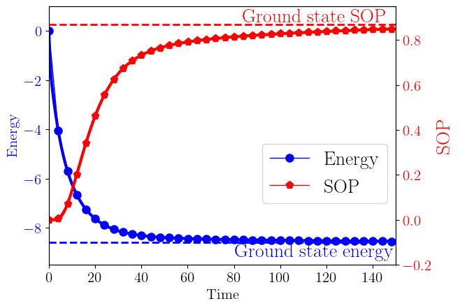
Figure 14: Energy and string order parameter (SOP) during the evolution for the non-integrable cluster state Hamiltonian (32) under boundary dissipation with system size $N=10$. The plot shows the energy converging to the ground state energy and the SOP transitioning from the paramagnetic phase (SOP $=0$) to the symmetry-protected topological (SPT) phase.

VII Rapid ground state preparation of weakly interacting spin systems

Our numerical results in Section VI strongly suggest that dissipative dynamics can achieve rapid mixing, or $\mathcal{O}(\log N)$ mixing time, for certain non-commuting Hamiltonians under bulk dissipation. However, as discussed in Section I, despite significant progress in theoretical understanding of the effectiveness of finite-temperature quantum Gibbs samplers [62, 35, 4, 56, 20, 36, 57, 66], many of these techniques cannot be used to characterize the convergence towards the ground state due to its singular nature. In this section, we develop a technique that provides the first rapid mixing result for a class of general non-commuting Hamiltonians.

We focus on the Lindbladian dynamics without coherent terms, i.e.

$$\frac{\mathrm{d}\rho}{\mathrm{d}t}=\mathcal{L}[\rho]=\sum_{a}\underbrace{K_{a}\rho K_{a}^{\dagger}-\frac{1}{2}\left\{K_{a}^{\dagger}K_{a},\rho\right\}}_{:=\mathcal{L}_{a,\varepsilon}}.$$ (33)

For concreteness, consider a local Hamiltonian $H$ over a $D$-dimensional lattice of spin systems $\Lambda=[0,L]^{D}$ with the following form (the system size is $N=(L+1)^{D}$):

$$H=H_{0}+H_{1}=-\sum_{i}Z_{i}+\varepsilon\sum_{j}h_{j},\quad\|h_{j}\|\leq 1.$$ (34)

Here, $H_{0}=-\sum_{i}Z_{i}$ is referred to as the non-interacting term because its indices do not overlap. The choice of $Z_{i}$ as the non-interacting term is made for convenience, and can be substituted with other simple, gapped local terms that also have non-overlapping indices. In the interacting term $H_{1}$, we assume each $h_{j}$ is supported on a set of spins sites whose Manhattan diameter is at most $r_{0}$, and each site $i$ appears in at most $l$ non-trivial $h_{j}$ terms. The resulting Hamiltonian $H$ is called a $(r_{0},l)$-geometrically local Hamiltonian. A specific example of the Hamiltonian in Eq. 34 is the $D$-dimensional TFIM model, which is a $(2,2D+1)$-local Hamiltonian. The parameter $\varepsilon$ is called the interaction strength.

For the Hamiltonian (34), it is sufficient to choose $\{A_{a}\}=\{X_{i}\}_{i\in\Lambda}$ to be the set of all single Pauli $X$ matrices as coupling operators. This is because if the interaction strength $\varepsilon=0$, then the dissipative dynamics for the non-interacting problem is ergodic and and the mixing time scales as $\mathcal{O}(\log N)$. Our main result is that there exists a critical interaction strength $\varepsilon^{*}$ independent of $L$ (and thus $N$), so that for all $\varepsilon<\varepsilon^{*}$, the scaling of the mixing time remains $\mathcal{O}(\log N)$.

Theorem 2 (Informal).

Consider a gapped Hamiltonian $H$ in the form of (34) defined on a $D$-dimensional lattice $\Lambda=[0,L]^{D}$, and $N=(L+1)^{D}$ is the system size. Let $\{A_{a}\}=\{X_{i}\}_{i\in\Lambda}$ be a set of coupling operators and $\{K_{a}\}$ be the corresponding jump operators defined via Eq. 3. Consider the Lindblad operator without the coherent term (33). Then there exists a constant $\varepsilon^{*}$ independent of the system size such that when $\varepsilon<\varepsilon^{*}$, we have

$$\tau_{\operatorname{mix}}(\eta)=\Theta(\log(N/\eta))\,,$$ (35)

where $\tau_{\operatorname{mix}}(\eta)$ is defined in (4).

The rigorous statement of Theorem 2 and its proof are given in Appendix F. Our first observation is that the recent analysis of mixing times of quantum Gibbs samplers in the high-temperature regime [57] does not rely on the invertibility of the stationary state. Instead, it measures the progress of the dynamics using a quantity called the oscillator norm of observables, which can be defined for any ergodic Lindblad dynamics with a unique fixed point $\sigma$.

Specifically, the evolution of any observable $O$ in the Heisenberg picture follows the dynamics $O(t)=e^{\mathcal{L}^{\dagger}t}(O)$. Since $\mathcal{L}^{{\dagger}}(I)=0$ for any Lindbladian, if the Lindblad dynamics $\rho(t)=\exp(\mathcal{L}t)\rho$ has a unique fixed point, then the identity operator $I$ is also the unique fixed point of the dynamics $e^{\mathcal{L}^{\dagger}t}$. In other words, $\lim_{t\to\infty}O(t)=\chi_{O}I$ for some constant $\chi_{O}$. For a index set $\mathcal{A}\subseteq\Lambda$, define the local oscillation operator

$$\delta_{\mathcal{A}}(O):=O-\frac{1}{2^{|\mathcal{A}|}}I_{\mathcal{A}}\otimes\mathrm{Tr}_{\mathcal{A}}(O)\,,$$ (36)

where $\mathrm{Tr}_{\mathcal{A}}(O)$ is the partial trace of $O$ with respect to the indices in $\mathcal{A}$. Then $\delta_{\mathcal{A}}(O)$ measures the local deviation of $O$ from the identity. Furthermore, we expect that $\lim_{t\to\infty}\delta_{\mathcal{A}}(O(t))=0$ for any nonempty $\mathcal{A}$ and observable $O$. For a given index $i\in\Lambda$, for simplicity we identify $i$ with its singleton set $\{i\}$. Then Ref. [57] quantifies the convergence of the Lindblad dynamics by means of the convergence of the oscillator norm $\sum_{i\in\Lambda}\left\|\delta_{i}(O)\right\|$.

For ground state preparation, we first modify the definition of the oscillator norm as follows:

$${\left|\kern-1.07639pt\left|\kern-1.07639pt\left|O\right|\kern-1.07639pt\right|\kern-1.07639pt\right|}:=\sum_{i\in\Lambda}\left\|\delta_{i}\circ P_{i}(O)\right\|+\left\|\delta_{i}\circ Q_{i}(O)\right\|\,.$$ (37)

Here

$$P_{i}(O)=\left|0_{i}\right\rangle\left\langle 0_{i}\right|\left\langle 0_{i}\right|O\left|0_{i}\right\rangle+\left|1_{i}\right\rangle\left\langle 1_{i}\right|\left\langle 1_{i}\right|O\left|1_{i}\right\rangle\,,$$ (38)

and

$$Q_{i}(O)=\left|0_{i}\right\rangle\left\langle 1_{i}\right|\left\langle 0_{i}\right|O\left|1_{i}\right\rangle+\left|1_{i}\right\rangle\left\langle 0_{i}\right|\left\langle 1_{i}\right|O\left|0_{i}\right\rangle\,,$$ (39)

which will be used to measure the progress of the dynamics along the diagonal and off-diagonal directions, respectively.

Then using the characterization of the trace distance via observables, the trace distance between $\rho(t)$ and $\sigma=|\psi_{0}\rangle\langle\psi_{0}|$ can be bounded as

$$\left\|\rho(t)-\sigma\right\|_{1}=\sup_{\|O\|\leq 1}\mathrm{Tr}\left(O\left(\rho(t)-\sigma\right)\right)$$ (40)

$$\leq \sup_{\|O\|\leq 1}\left\|O(t)-\mathrm{Tr}(O(t))/2^{N}\right\|\left\|\rho(0)-\sigma\right\|_{1}$$

$$\leq \sup_{\|O\|\leq 1}{\left|\kern-1.07639pt\left|\kern-1.07639pt\left|O(t)\right|\kern-1.07639pt\right|\kern-1.07639pt\right|}\left\|\rho(0)-\sigma\right\|_{1}.$$

The key step is given in Proposition 10 in Appendix F, which proves that when $\varepsilon<\varepsilon^{*}$, the modified oscillator norm decays exponentially: ${\left|\kern-1.07639pt\left|\kern-1.07639pt\left|O(t)\right|\kern-1.07639pt\right|\kern-1.07639pt\right|}\leq\exp(-t/4){\left|\kern-1.07639pt\left|\kern-1.07639pt\left|O(0)\right|\kern-1.07639pt\right|\kern-1.07639pt\right|}\leq 4N\exp(-t/4)$ for any $\|O\|\leq 1$. The proof uses the Lieb-Robinson bound. This immediately yields the desired result in Theorem 2.

VIII Rapid ground state preparation of weakly interacting fermionic systems

In Theorem 2, the non-interacting Hamiltonian is defined as a sum of single-site Pauli $Z$ operators. In this section, we extend this result to the fermionic setting. Since free fermionic systems can be exactly diagonalized, we introduce a more general non-interacting term that permits coupling between fermionic sites.

We consider a local fermionic Hamiltonian $H$ defined on a $D$-dimensional lattice of fermionic systems, $\Lambda=[0,L]^{D}$, given by

$$H_{\varepsilon}=H_{0}+H_{1}=\sum_{ij}M_{i,j}c^{\dagger}_{i}c_{j}+\varepsilon\sum_{j}h_{j},$$ (41)

where $(M_{i,j})$ is a positive definite Hermitian matrix, and $c^{\dagger}_{j}$ and $c_{j}$ are the creation and annihilation operators at site $j$. The terms $h_{j}$ represent local fermionic perturbations satisfying $\|h_{j}\|_{\infty}\leq 1$ and preserving parity, meaning each $h_{j}$ contains an even number of creation and annihilation operators. We further assume that $H_{0}$ is $(1,l)$-geometrically local and $\sum_{j}h_{j}$ are $(r_{0},l)$-geometrically local. Specifically, each term in $H_{0}$ is a product of fermionic operators acting on a set of sites whose Manhattan diameter is at most $1$, and each $h_{j}$ is a product of fermionic operators acting on a set of sites whose Manhattan diameter is at most $r_{0}$. In addition, each site $i$ appears in at most $l$ non-trivial $c^{\dagger}_{i}c_{j}$ and $h_{j}$ terms.

For Eq. 41, we choose $\{A_{a}\}=\{c^{\dagger}_{i},c_{i}\}_{i\in\Lambda}$ to be the set of all single fermionic operators as coupling operators. We show that the mixing time of the Lindblad dynamics for the fermionic system (41) also scales logarithmically with the system size for sufficiently small $\varepsilon$. This is summarized in the following theorem:

Theorem 3 (Informal).

Consider a gapped fermionic Hamiltonian $H$ in the form of (41) defined on a $D$-dimensional lattice $\Lambda=[0,L]^{D}$, and $N=(L+1)^{D}$ is the system size. Let $\{A_{a}\}=\{c^{\dagger}_{i},c_{i}\}_{i\in\Lambda}$ be a set of coupling operators and $\{K_{a}\}$ be the corresponding jump operators defined via Eq. 3. Consider the Lindblad operator without the coherent term (33). Then there exists a constant $\varepsilon^{*}$ independent of the system size such that when $\varepsilon<\varepsilon^{*}$, we have

$$\tau_{\operatorname{mix}}(\eta)=\Theta(\log(N/\eta))\,,$$ (42)

where $\tau_{\operatorname{mix}}(\eta)$ is defined in (4).

The creation and annihilation operators are non-local in the spin basis after applying the Jordan–Wigner transformation. As a result, the oscillator norm defined in Eq. 37 is not suitable for fermionic systems. A proper definition of the oscillator norm requires the notion of the fermionic partial trace that is compatible with the canonical anticommutation relation (CAR).

We introduce a shorthand notation $\left|1_{i}\right\rangle=c^{\dagger}_{i}\left|\mathrm{vac}\right\rangle$ and $\left|0_{i}\right\rangle=c_{i}c_{i}^{{\dagger}}\left|\mathrm{vac}\right\rangle$ for all $i$. Then with some abuse of notation, we require that $c_{j},c_{j}^{{\dagger}}$ “anticommutes” with $\left|1_{i}\right\rangle,\left\langle 1_{i}\right|$ for all $i\neq j$, and “commutes” with $\left|0_{i}\right\rangle,\left\langle 0_{i}\right|$ for all $i\neq j$. For instance, consider $O=c_{1}^{{\dagger}}c_{2}^{{\dagger}}c_{2}c_{3}$, then

$$\braket{1_{2}|O|1_{2}}=(-1)^{2}c_{1}^{{\dagger}}\braket{1_{2}|c_{2}^{{\dagger}}c_{2}|1_{2}}c_{3}=c_{1}^{{\dagger}}c_{3}.$$ (43)

Here the factor $(-1)^{2}$ is due to the convention that $\left\langle 1_{2}\right|$ is required to anticommute with $c_{1}^{{\dagger}}$, and $\left|1_{2}\right\rangle$ is required to anticommute with $c_{3}$. This is analogous to operations in spin systems, where commuting a state past spin operators acting on different sites follows a similar rule. For example, in a two-site system, we can rewrite $X_{1}X_{2}\left|1_{1}\right\rangle=X_{1}\left|1_{1}\right\rangle X_{2}$, treating the operators sequentially while preserving their site-specific action.

More generally, for any observable $O$, the fermionic partial trace on the $i$-th lattice, denoted by $\mathrm{Tr}^{f}_{i}$, can be defined as:

$$\mathrm{Tr}^{f}_{i}(O)=\left\langle 0_{i}\right|O\left|0_{i}\right\rangle+\left\langle 1_{i}\right|O\left|1_{i}\right\rangle.$$ (44)

The tensor product with the identity matrix in (36) now takes the form

$$\mathsf{T}_{i}\left(O\right)=\frac{c^{\dagger}_{i}c_{i}+c_{i}c^{\dagger}_{i}}{2}\mathrm{Tr}^{f}_{i}(O)\,,$$ (45)

where we have used that $c^{\dagger}_{i}c_{i}+c_{i}c^{\dagger}_{i}=1$ is even in the fermionic operators and commutes with all $c_{j},c_{j}^{{\dagger}}$ when $i\neq j$. The fermionic local oscillation operator is then defined as

$$\delta^{f}_{i}(O)=O-\mathsf{T}_{i}(O)\,.$$ (46)

Following the fermionic notation convention above, we may generalize the definition of $P_{i},Q_{i}$ in (38) and (39) to fermionic systems. Due to the fact the even parity of the density operator $\rho$, which implies that $\mathrm{Tr}(O\rho)=0$ if $O$ has odd parity, we only consider even parity observable in our analysis. We can define the fermionic oscillator norm as

$${\left|\kern-1.07639pt\left|\kern-1.07639pt\left|O\right|\kern-1.07639pt\right|\kern-1.07639pt\right|}:=\sum^{N}_{i=1}\left\|\delta^{f}_{i}\circ P_{i}(O)\right\|_{\infty}+\left\|\delta^{f}_{i}\circ Q_{i}(O)\right\|_{\infty}\,.$$ (47)

We note that several alternative expressions for the fermionic partial trace exist in the literature (see, e.g., [13, 72]). However, we emphasize that the fermionic partial trace operation is uniquely defined once the ordering of the sites is fixed and the fermionic states satisfy the parity superselection rule (SSR), i.e., a fermionic state should not involve a coherent superposition between states with an even and an odd number of particles.

Finally, we summarize the properties of the fermionic partial trace (45) and the fermionic local oscillation operator (46) in the following.

1. The fermionic partial trace operators $\{\mathsf{T}_{i}\}$ commute with each other, meaning $\mathsf{T}_{i}\circ\mathsf{T}_{j}\left(O\right)=\mathsf{T}_{j}\circ\mathsf{T}_{i}\left(O\right)$.

2. The fermionic partial trace is contractive in operator norm, meaning $\|\mathsf{T}_{i}\|_{\infty\rightarrow\infty}\leq 1$.

3. The fermionic local oscillation operator can control the convergence of observables.

   Lemma 4.

   For any observable $O$ that takes the form of (115), we have

   $$\left\|O-I/2^{N}\mathrm{Tr}(O)\right\|_{\infty}\leq\sum^{N}_{i}\|\delta^{f}_{i}(O)\|_{\infty}\,.$$

4. The fermionic partial trace and local fermionic oscillation operator commute with operators that act on different sites:

   Lemma 5.

   Given any superoperator $\mathcal{F}$:

   $$\mathcal{F}(O)=a_{1}a_{2}\cdots a_{l}Ob_{1}b_{2}\cdots b_{r}\,,$$ (48)

   where $a_{i},b_{i}\in\{c_{i},c^{\dagger}_{i}\}_{i\in I}$. If $l+r$ is an even number, $j\notin I$, and $O$ has even parity, $[\mathcal{F},\mathsf{T}_{j}](O)=0$ and $\left[\mathcal{F},\delta^{f}_{j}\right](O)=0$.

   According to the above lemma, it is straightforward to see that $\mathcal{L}^{\dagger}_{i,\varepsilon}$ commutes with $\delta^{f}_{j}$ if the site $j$ is not within the fermionic support of $\mathcal{L}^{\dagger}_{i,\varepsilon}$.

5. The fermionic partial trace generates the local fixed point for local Lindbladian operators:

   Lemma 6.

   Assume $\mathcal{L}^{\dagger}$ can be written into the summations of  (48) such that every term satisfies the conditions of Lemma 5. Given a subset $J\in\{1,\dots,N\}$ and an observable $O$ that has even parity, if $I\subset J$, we have $\mathcal{L}(\mathsf{T}_{J}(O))=0$, where $\mathsf{T}_{J}(O)=\Pi_{i\in J}\mathsf{T}_{i}(O)$.

The proof of these claims and lemmas will be given in Appendix G.3 for completeness. Using these properties the proof of Theorem 3 can follow a similar strategy in the spin case. We provide the rigorous version of Theorem 3, the technical details, and the proof of it in Appendix G.

Additionally, we note that in both Theorems 2 and 3, the perturbation terms are assumed to be local for simplicity. Our results can be naturally extended to quasi-local perturbations.

IX Discussion

This work significantly strengthens the evidence of the power of dissipative dynamics in preparing ground states for a wide class of non-commuting Hamiltonians. A variety of dissipative mechanisms exist, such as imaginary-time evolution (ITE) [45, 48, 32]. However, implementing ITE via the operator $e^{-\tau H}$ does not readily yield a completely positive trace-preserving (CPTP) map. Existing approaches often rely on variational ansatze or tomography-based procedures. By contrast, Lindblad dynamics provides a non-variational and inherently CPTP process that can be efficiently implemented on fault-tolerant quantum hardware.

We have shown that a carefully designed Lindblad dynamics succeeds in preparing the ground states of quadratic Majorana Hamiltonians, and have proven its effectiveness for non-integrable but weakly interacting spin Hamiltonians. Our tensor-network simulations suggest that these methods can remain effective beyond the reach of our rigorous analysis. For fermionic systems, our Theorem 3 generalizes the recent work of [66], which establishes the spectral gap for Gibbs state preparation in perturbed fermionic systems. Our result extends this to the ground state (zero temperature). Our result enhances the spectral gap bound (also called fast mixing) at finite temperatures from Ref. [66] to the stronger notion of rapid mixing, and proves rapid mixing at zero temperature. It is worth noting that Theorem 3 still imposes certain restrictions on the choice of the non-interacting term. Removing these restrictions and extending our result to efficient low-temperature thermal state preparation remain interesting directions for future work. Additionally, investigating spin systems with long-range interactions may provide further insights into the mixing properties of dissipative processes.

A key open question is whether dissipative dynamics can tackle classically hard ground-state problems. We also note that, in the perturbative regime of non-interacting systems, the ground states can likely be prepared efficiently using alternative quantum algorithms, such as quantum adiabatic evolution. On the other hand, viewing ground-state preparation as a minimization problem, there exist instances where finding even a local minimum is classically hard, yet Lindblad dynamics can efficiently achieve this quantumly [12]. In the case of [12], the local and global minima coincide, resulting in a single-phase ground state. Many challenging physical Hamiltonians involve resolving multiple phases with nearly degenerate energy levels, which typically lie outside the perturbative regime. A prominent example is the phase diagram of the two-dimensional Hubbard model. Further theoretical analysis and tensor-network based simulations may be instrumental in quantifying the scope of the quantum advantage in these more complex scenarios.

Acknowledgments– This material is based upon work supported by the U.S. Department of Energy, Office of Science, Accelerated Research in Quantum Computing Centers, Quantum Utility through Advanced Computational Quantum Algorithms, grant no. DE-SC0025572 (J.P., G.K.C., L.L.). Additional support is acknowledged from the U.S. Department of Energy, Office of Science, National Quantum Information Science Research Centers, Quantum Systems Accelerator (Y.Z., Z.D., J.P., L.L.) and the National Science Foundation, grant no. PHY-2317110 (Y.Z., J.P.). The Institute for Quantum Information and Matter is an NSF Physics Frontiers Center. L.L. is a Simons Investigator in Mathematics. This research used the Savio computational cluster resource provided by the Berkeley Research Computing program at the University of California, Berkeley. Z.D., J.H. and L.L. thank the Institute for Pure and Applied Mathematics (IPAM) for its hospitality in hosting them as long-term visitors during the semester-long program “Mathematical and Computational Challenges in Quantum Computing” in Fall 2023, from which this collaboration started. The authors thank Joao Basso, Paul Cazeaux, Anthony Chen, Soonwon Choi, Marius Junge, Michael Kastoryano, Jianfeng Lu, Christian Mendl, Gunhee Park, Cambyse Rouzé, Yu Tong for helpful discussions.

Author contributions– G.K.C. and L.L. conceived the original study. Y.Z., Z.D., and L.L. carried out theoretical analysis to support the study. Y.Z., J.H. and L.L. carried out numerical calculations to support the study. J.G. provided support in tensor network-based simulations. All authors, Y.Z., Z.D., J.H., J.G., J.P., G.K.C., and L.L. discussed the results of the manuscript and contributed to the writing of the manuscript.

Appendix A Notation

For a matrix $A\in\mathbb{C}^{N\times N}$, let $A^{*},A^{T},A^{{\dagger}}$ be the complex conjugation, transpose, and Hermitian transpose (or adjoint) of $A$, respectively. Unless specified otherwise, $\left\lVert A\right\rVert\equiv\left\lVert A\right\rVert_{\infty}$ denotes the operator norm, and $\left\lVert A\right\rVert_{1}=\mathrm{Tr}(\sqrt{A^{\dagger}A})$ denotes the $1$-norm or the trace norm. The trace distance between two states $\rho,\sigma$ is $D(\rho,\sigma):=\frac{1}{2}\left\lVert\rho-\sigma\right\rVert_{1}$. We write $A\succeq 0$ (resp., $A\succ 0$) for a positive semidefinite (resp., definite) matrix, $A\succeq B$ if $A-B\succeq 0$, and $A\preceq B$ if $B\succeq A$.

We adopt the following asymptotic notations beside the usual big $\mathcal{O}$ one. We write $f=\Omega(g)$ if $g=\mathcal{O}(f)$; $f=\Theta(g)$ if $f=\mathcal{O}(g)$ and $g=\mathcal{O}(f)$. The notations $\widetilde{\mathcal{O}}$, $\widetilde{\Omega}$, $\widetilde{\Theta}$ are used to suppress subdominant polylogarithmic factors. Specifically, $f=\widetilde{\mathcal{O}}(g)$ if $f=\mathcal{O}(g\operatorname{polylog}(g))$; $f=\widetilde{\Omega}(g)$ if $f=\Omega(g\operatorname{polylog}(g))$; $f=\widetilde{\Theta}(g)$ if $f=\Theta(g\operatorname{polylog}(g))$. Note that these tilde notations do not remove or suppress dominant polylogarithmic factors. For instance, if $f=\mathcal{O}(\log g\log\log g)$, then we write $f=\widetilde{\mathcal{O}}(\log g)$ instead of $f=\widetilde{\mathcal{O}}(1)$.

Appendix B Quasi-free systems

Jordan–Wigner transformation—

Following the convention in [51], we introduce the following Jordan-Wigner transformation for fermionic annihilation and creation operators

$$c_{j}=\left(\prod_{k=1}^{j-1}Z_{k}\right)X_{j}^{-}=X_{j}^{-}\left(\prod_{k=1}^{j-1}Z_{k}\right),\quad c_{j}^{\dagger}=X_{j}^{+}\left(\prod_{k=1}^{j-1}Z_{k}\right)=\left(\prod_{k=1}^{j-1}Z_{k}\right)X_{j}^{+},$$ (49)

with

$$X_{j}^{-}=\frac{1}{2}(X_{j}-iY_{j}),\quad X_{j}^{+}=\frac{1}{2}(X_{j}+iY_{j}).$$ (50)

Here $X_{-}$ and $X_{+}$ are called the lowering and raising operators. After the Jordan-Wigner transformation,

$$X_{j}X_{j+1}=X_{j}Z_{j}\left(\prod_{k=1}^{j-1}Z_{k}\right)(c_{j+1}^{{\dagger}}+c_{j+1})=-iY_{j}\left(\prod_{k=1}^{j-1}Z_{k}\right)(c_{j+1}^{{\dagger}}+c_{j+1})=(c_{j}-c^{{\dagger}}_{j})(c_{j+1}^{{\dagger}}+c_{j+1}).$$ (51)

Then the 1D TFIM Hamiltonian in (5)

$$H=-g\sum_{i=1}^{N}Z_{i}-J\sum_{i=1}^{N-1}X_{i}X_{i+1}$$

can be expressed as

$$H=-J\sum_{j=1}^{N-1}(c_{j}-c^{{\dagger}}_{j})(c_{j+1}^{{\dagger}}+c_{j+1})-2g\sum_{j=1}^{N}c_{j}^{{\dagger}}c_{j}+gN.$$ (52)

We now perform a unitary rotation

$$\binom{c_{j}}{c_{j}^{\dagger}}=\frac{1}{\sqrt{2}}\left(\begin{array}[]{cc}1&-i\\ 1&i\end{array}\right)\binom{w_{j}}{w_{j+N}},\quad j=1,\ldots,N.$$ (53)

This defines a set of $2N$ Majorana operators, $\left\{w_{p}\right\}_{p=1}^{2N}$, which are Hermitian operators satisfying the anticommutation relation

$$\left\{w_{p},w_{q}\right\}:=w_{p}w_{q}+w_{q}w_{p}=\delta_{pq},\quad p,q=1,\ldots,2N.$$ (54)

This gives rise to the Majorana form of the Hamiltonian in Eq. 6:

$$H=2iJ\sum_{j=1}^{N-1}w_{j+N}w_{j+1}+2ig\sum_{j=1}^{N}w_{j}w_{j+N}.$$

Quadratic Majorana systems—

The general form of a quadratic Majorana Hamiltonian with $2N$ modes is:

$$H=2\sum_{1\leq p<q\leq 2N}h_{pq}w_{p}w_{q}=\sum_{p,q=1}^{2N}h_{pq}w_{p}w_{q},$$ (55)

The coefficient matrix $h$ is Hermitian and purely imaginary. In other words, we may write $h=-i\mathsf{A}$, where $\mathsf{A}$ is a real antisymmetric matrix. The eigenvalues of the coefficient matrix $h$ are thus real and symmetric with respect to $0$. Let $\{\lambda_{k}\}_{k=1}^{N}$ be the positive eigenvalues of $h$, and $\Delta=\min_{k}\lambda_{k}$ is called the spectral gap. Then after a unitary transformation followed by a particle-hole transformation, we may write

$$H=\sum_{k=1}^{N}\lambda_{k}(b_{k}^{{\dagger}}b_{k}+b^{{\dagger}}_{k+N}b_{k+N})-\sum_{k=1}^{N}\lambda_{k}.$$ (56)

Here $\{b_{k},b_{k}^{{\dagger}}\}_{k=1}^{2N}$ is a set of fermionic annihilation and creation operators satisfying the canonical anticommutation relation (CAR), and is linear in the fermionic operators $\{c_{j},c_{j}^{{\dagger}}\}$ in Eq. 53. The ground state is the quasi-vacuum state satisfying (see e.g. [6, Chapter 3])

$$b_{k}\left|\mathrm{vac}\right\rangle=0,\quad k=1,\ldots,2N.$$ (57)

Quasi-free dynamics—

We consider a general non-interacting quadratic Hamiltonian $H=\sum_{i,j=1}^{2N}h_{ij}w_{i}w_{j}$. According to the Thouless theorem [65],

$$e^{\mathrm{i}Hs}w_{a}e^{-\mathrm{i}Hs}=\sum_{p}w_{p}\left(e^{-2\mathrm{i}h}\right)_{ap}.$$ (58)

As a result, the jump operator associated with a coupling operator $w_{a}$ is a linear combination of Majorana operators

$$K_{a} =\int_{\mathbb{R}}f(s)e^{\mathrm{i}Hs}w_{a}e^{-\mathrm{i}Hs}\mathrm{d}s$$ (59)

$$=\sum_{p}\int_{\mathbb{R}}f(s)\left(e^{-\mathrm{i}2hs}\right)_{ap}w_{p}\mathrm{d}s$$

$$=\sum_{p}[\hat{f}(-2h)]_{ap}w_{p}.$$

Then if the set of coupling operators is $\{A_{a}=w_{a}\}_{a\in\mathcal{I}}$ where $\mathcal{I}$ is some index set, a closed-form equation for the covariance matrix $\Gamma_{p,q}:=\frac{i}{2}\left\langle w_{p}w_{q}-w_{q}w_{p}\right\rangle$ can be derived as [5, Proposition 1]:

$$\partial_{t}\Gamma=X\Gamma+\Gamma X^{T}+Y,\quad X=-2ih-B_{\text{real}},\quad Y=B_{\text{imag}},$$ (60)

Here the coefficient matrix

$$B_{pq}=\sum_{a\in\mathcal{I}}\left[\hat{f}(-2h)\right]_{ap}\left[\hat{f}(-2h)\right]_{aq}^{*}.$$ (61)

Here, $B$ is the sum over all the coefficients of the jump operators, with $B_{\text{real}}$, $B_{\text{imag}}$ denoting the (entry-wise) real and imaginary parts of $B$, respectively. Since the filter function $\hat{f}(\omega)$ is only supported on the negative real axis, the Lindbladian dynamics filters out all positive eigenmodes of $h$ while simultaneously populating the negative modes, which contributes to the ground state of the quadratic Hamiltonian $H$.

Appendix C Mixing time of quasi-free systems and proof of Theorem 21

After the canonical unitary transformation and the particle hole transformation, we express the quadratic Hamiltonian $H$ in the canonical form of (56). We also define

$$\lambda_{k+N}=\lambda_{k},\quad 1\leq k\leq N.$$ (62)

Let $\hat{n}_{k}=b_{k}^{{\dagger}}b_{k}$ be the number operator of the $k$-th mode, and $\hat{N}=\sum_{k}\hat{n}_{k}=\mathbf{b}^{{\dagger}}\mathbf{b}$ be the total number operator. Note that all creation operators $b_{k}^{{\dagger}}$ increases the energy, while all annihilation operators $b_{k}$ decreases the energy. As a result, the jump operator must be a linear combination of annihilation operators alone:

$$K_{a}=\sum_{p=1}^{2N}\Phi^{*}_{pa}b_{p}$$ (63)

for some coefficient matrix $\Phi$, so that $K_{a}\left|\mathrm{vac}\right\rangle=0$.

Define $O=\sum_{k,l=1}^{2N}\Xi_{kl}b^{{\dagger}}_{k}b_{l}$ for some positive definite matrix $\Xi$ to be determined. Then

$$i[H,O]=i\sum_{k}\lambda_{k}[n_{k},O]=i\sum_{kl}(\lambda_{k}-\lambda_{l})\Xi_{kl}b_{k}^{{\dagger}}b_{l}.$$ (64)

We may also directly compute

$$\begin{split}&\sum_{a}K_{a}^{{\dagger}}OK_{a}-\frac{1}{2}\{K^{{\dagger}}_{a}K_{a},O\}=\frac{1}{2}\sum_{a}(K^{{\dagger}}_{a}[O,K_{a}]-[O,K^{{\dagger}}_{a}]K_{a})\\ =&-\frac{1}{2}\sum_{a}\left(\sum_{p}\Phi_{pa}b^{{\dagger}}_{p}\sum_{kl}\Xi_{kl}\Phi_{ka}^{*}b_{l}+\sum_{kl}\Xi_{kl}\Phi_{la}b_{k}^{{\dagger}}\sum_{p}\Phi_{pa}^{*}b_{p}\right)\\ =&-\frac{1}{2}\sum_{kl}b_{k}^{{\dagger}}\left(\sum_{ap}\Phi_{ka}\Phi_{pa}^{*}\Xi_{pl}+\Xi_{kp}\Phi_{pa}\Phi_{la}^{*}\right)b_{l}.\end{split}$$ (65)

Let $h=\operatorname{diag}(\{\varepsilon_{p}\})$, and define a non-Hermitian Hamiltonian (the superscript $f$ means the non-Hermitian matrix is defined with respect to fermionic creation and annihilation operators instead of Majorana operators):

$$H_{\mathrm{nh}}=iH-\frac{1}{2}\sum_{a}K_{a}^{{\dagger}}K_{a}=\mathbf{b}^{{\dagger}}h^{f}_{\mathrm{nh}}\mathbf{b},\quad h^{f}_{\mathrm{nh}}=ih-\frac{1}{2}\Phi\Phi^{{\dagger}},$$ (66)

then

$$\mathcal{L}^{{\dagger}}[O]=\mathbf{b}^{{\dagger}}\left[\left(ih-\frac{1}{2}\Phi\Phi^{{\dagger}}\right)\Xi+\Xi\left(-ih-\frac{1}{2}\Phi\Phi^{{\dagger}}\right)\right]\mathbf{b}=\mathbf{b}^{{\dagger}}(h^{f}_{\mathrm{nh}}\Xi+\Xi(h^{f}_{\mathrm{nh}})^{{\dagger}})\mathbf{b}.$$ (67)

Here the coefficient matrix $h^{f}_{\mathrm{nh}}$ is related to that in Eq. 19 by a similarity transformation.

Under the assumption that $h^{f}_{\mathrm{nh}}$ can be diagonalized into $VDV^{-1}$ for some invertible matrix $V$ and diagonal matrix $D$, we now make a choice of the Hermitian matrix $\Xi=VV^{{\dagger}}\succ 0$. Let $\Delta=-\max_{i}\operatorname{Re}D_{ii}$ be the non-Hermitian gap. Then

$$\mathcal{L}^{{\dagger}}[O]=\mathbf{b}^{{\dagger}}V(D+D^{*})V^{{\dagger}}\mathbf{b}\preceq-2\Delta\mathbf{b}^{{\dagger}}VV^{{\dagger}}\mathbf{b}=-2\Delta O.$$ (68)

This immediately yields the exponential convergence of the observable $O$ as

$$\mathrm{Tr}[O\rho(t)]\leq\mathrm{Tr}[O\rho(0)]e^{-2\Delta t}.$$ (69)

From the definition of $\Xi$ we have

$$\lambda_{\min}(VV^{{\dagger}})\hat{N}\preceq O\preceq\lambda_{\max}(VV^{{\dagger}})\hat{N}.$$ (70)

Then the infidelity can be bounded as

$$\begin{split}1-\braket{\mathrm{vac}|\rho|\mathrm{vac}}\leq\mathrm{Tr}[\hat{N}\rho]\leq&\frac{1}{\lambda_{\min}(VV^{{\dagger}})}\mathrm{Tr}[O\rho]\leq\frac{1}{\lambda_{\min}(VV^{{\dagger}})}\mathrm{Tr}[O\rho(0)]e^{-2\Delta t}\\ \leq&\frac{\lambda_{\max}(VV^{{\dagger}})}{\lambda_{\min}(VV^{{\dagger}})}\mathrm{Tr}[\mathbf{c}^{{\dagger}}\mathbf{c}\rho(0)]e^{-2\Delta t}=\kappa^{2}(V)\mathrm{Tr}[\hat{N}\rho(0)]e^{-2\Delta t}.\end{split}$$ (71)

Finally by the Fuchs–van de Graaf inequality,

$$D(\rho,|\mathrm{vac}\rangle\!\langle\mathrm{vac}|)\leq\sqrt{1-\braket{\mathrm{vac}|\rho|\mathrm{vac}}}\leq\kappa(V)\sqrt{\mathrm{Tr}[\hat{N}\rho(0)]}e^{-\Delta t}.$$ (72)

Finally, we use $\mathrm{Tr}[\hat{N}\rho(0)]\leq 2N$ for any initial state $\rho(0)$ and finish the proof of Theorem 21.

Appendix D Mixing time of 1D TFIM with boundary dissipation

To simplify the analysis we adopt the “c-cyclic” approximation in [41, 51], and consider the following periodized version of the TFIM Hamiltonian expressed in fermionic operators

$$H_{\mathrm{per}}=-J\sum_{j=1}^{N-1}(c_{j}-c^{{\dagger}}_{j})(c_{j+1}^{{\dagger}}+c_{j+1})-J\left(c_{N}-c_{N}^{\dagger}\right)\left(c_{1}^{\dagger}+c_{1}\right)-2g\sum_{j=1}^{N}c_{j}^{{\dagger}}c_{j}+gN.$$ (73)

Compared to Eq. 52, this Hamiltonian introduces a periodic term. Define the ratio $\xi=J/g$. When $\xi\neq 1$, the modified Hamiltonian is gapped, and can be exactly diagonalized as

$$H_{\rm per,c}=2g\sum_{k}\Lambda_{k}b_{k}^{{\dagger}}b_{k}-g\sum_{k}\Lambda_{k}.$$ (74)

Here for convenience we assume $N$ is even, and label the eigenvalues from $-\frac{N}{2}$ to $\frac{N}{2}-1$, with

$$\Lambda_{k}=\sqrt{1+\xi^{2}+2\xi\cos\left(\frac{2\pi k}{N}\right)},\quad k=-\frac{N}{2},\ldots,\frac{N}{2}-1,$$ (75)

which is even with respect to the index $k$. The annihilation operators $\{b_{k}\}$ are given in the form of a Nambu spinor

$$b_{k}=\sum_{j}\left\{\left(\frac{\varphi_{kj}+\psi_{kj}}{2}\right)c_{j}+\left(\frac{\varphi_{kj}-\psi_{kj}}{2}\right)c_{j}^{{\dagger}}\right\},$$ (76)

with coefficients

$$\varphi_{kj}=\begin{cases}(2/N)^{1/2}\sin\left(\frac{2\pi jk}{N}\right)&k=1,\ldots,\frac{N}{2}-1\\ (2/N)^{1/2}\cos\left(\frac{2\pi jk}{N}\right)&k=-\frac{N}{2},\ldots,0\end{cases}$$ (77)

and

$$\psi_{kj}=-\Lambda_{k}^{-1}\left[\left(1+\xi\cos\left(\frac{2\pi k}{N}\right)\right)\varphi_{kj}+\xi\sin\left(\frac{2\pi k}{N}\right)\varphi_{-k,j}\right].$$ (78)

Direct calculation shows

$$X_{1}=c_{1}+c_{1}^{{\dagger}}=\sum_{k}\varphi_{k1}(b_{k}+b_{k}^{{\dagger}}),\quad Y_{1}=i(c_{1}-c_{1}^{{\dagger}})=\sum_{k}\psi_{ki}i(b_{k}-b_{k}^{{\dagger}}).$$ (79)

For ground state preparation, the corresponding jump operators simply filter out the energy-increasing $b_{k}^{{\dagger}}$ components:

$$K_{X_{1}}=\int f(s)e^{iHs}X_{1}e^{-iHs}\,\mathrm{d}s=\sum_{k}\varphi_{k1}b_{k},\quad K_{Y_{1}}=\int f(s)e^{iHs}Y_{1}e^{-iHs}\,\mathrm{d}s=\sum_{k}\psi_{k1}b_{k}.$$ (80)

The non-Hermitian Hamiltonian in Theorem 21 can be written as

$$H_{\rm nh}=\mathbf{b}^{{\dagger}}h_{\mathrm{nh}}^{f}\mathbf{b},\quad h^{f}_{\mathrm{nh}}=i\Lambda-\frac{1}{2}\varphi\varphi^{{\dagger}}-\frac{1}{2}\psi\psi^{{\dagger}}.$$ (81)

Note that the magnitudes of $\left\lvert\varphi_{kj}\right\rvert,\left\lvert\psi_{kj}\right\rvert$ vanish at least as $\mathcal{O}(N^{-\frac{1}{2}})$ for large system sizes. This allows us to use first order perturbation theory to estimate the non-Hermitian gap. For $k=0$, we have $\lambda_{0}=1+\xi$,

$$\frac{1}{2}\left(\varphi_{0,1}^{2}+\psi_{0,1}^{2}\right)=\frac{2}{N},$$ (82)

which is large compared to $\mathcal{O}(N^{-3})$. Due to the modification to periodic boundary conditions, every eigenvalue $\Lambda_{k}$ with $k>0$ is doubly degenerate with $\Lambda_{k}=\Lambda_{-k}$. This relation also approximately holds for the original TFIM problem with open boundary conditions. So we apply the perturbation theory to each two dimensional space spanned by the eigenvectors corresponding to the eigenvalue $\Lambda_{k}=\Lambda_{-k}$. Then

$$\Delta\approx\frac{1}{2}\min_{k>0}\lambda_{\min}(M_{k}),\quad M_{k}=\begin{pmatrix}\varphi_{k,1}^{2}+\psi_{k,1}^{2}&\varphi_{k,1}\varphi_{-k,1}+\psi_{k,1}\psi_{-k,1}\\ \varphi_{k,1}\varphi_{-k,1}+\psi_{k,1}\psi_{-k,1}&\varphi_{-k,1}^{2}+\psi_{-k,1}^{2}\end{pmatrix}.$$ (83)

For each $0<k<N/2$, we have

$$\det M_{k}=(\varphi_{k,1}\psi_{-k,1}-\varphi_{-k,1}\psi_{k,1})^{2}=\frac{\xi^{2}\sin^{2}\left(\frac{2\pi k}{N}\right)}{\Lambda_{k}^{2}}\left(\varphi_{k,1}^{2}+\varphi^{2}_{-k,1}\right)^{2}=\frac{4\xi^{2}\sin^{2}\left(\frac{2\pi k}{N}\right)}{N^{2}\Lambda_{k}^{2}}=\Omega(N^{-4}).$$ (84)

Therefore each $M_{k}$ is invertible and the spectral gap is positive. In particular, when $k=1$, $\det M_{k}=\Theta(N^{-4})$, and the magnitude of the entries are

$$M_{1}=\begin{pmatrix}\Theta(N^{-3})&\Theta(N^{-2})\\ \Theta(N^{-2})&\Theta(N^{-1}).\end{pmatrix}$$ (85)

Therefore one of the eigenvalues must be $\Theta(N^{-1})$. To obtain $\det M_{k}=\Theta(N^{-4})$, the other eigenvalue must be $\Theta(N^{-3})$.

Appendix E Additional numerical results on tensor network simulation

A key part of simulating the Lindbladian evolution is the compression of a sum of $M$ triple MPO products to a single MPO of bond dimension $D$ on $N$ sites, as described in Section V. A direct method contracts the three tensors per site for each term, then explicitly sums the $M$ terms, yielding a single MPO with bond dimension $MD^{3}$ which can be compressed using a sweep of QR decompositions and singular value truncations. The cost of this direct method scales as $\mathcal{O}(NM^{3}D^{9})$.

An alternative option would be to interleave compressions and contractions, that is, immediately compress back to bond dimension $D$ after every pairwise MPO multiplication or addition. Such an approach has a better scaling of $\mathcal{O}(NMD^{6})$. However, this approach can introduce a significantly larger error, as the number of compressions performed is $\mathcal{O}(NM)$ rather than $\mathcal{O}(N)$ in the previous case.

To resolve this problem, we employ the fitting method [68], which iteratively constructs the optimal (in terms of Frobenius norm) 1D approximation of a tensor network using only the overlap between the ansatz and the target network. Since the target is a linear sum of terms, each overlap can be calculated separately. This leads to a scaling of $\mathcal{O}(KMND^{5})$ with $K$ the number of sweeps required to converge the fitting procedure (typically $<20$). The library quimb [30] enables the fitting of a sum of such MPO products terms to a single MPO. It also supports the use of GPUs, which can greatly speed up the computations dominated by linear algebra operations such as this fitting routine. We report the results in Fig. 15.

To demonstrate the accuracy of the fitting method, we calculate $\mathrm{Tr}(HK_{a}\rho_{t=0.1}K_{a}^{\dagger})$ from the bulk-dissipated 1D-TFIM model with $J=1$ and $g=1.5$, and compress the triple MPO product $K_{a}\rho K_{a}^{\dagger}$ using the direct method and the fitting method. Here $K_{a}$ is the jump operator with coupling operator $X$ at the fifth site and $\rho_{t=0.1}$ is the density matrix at $t=0.1$ obtained from the Lindblad dynamics using a bond dimension of $50$. Then, $K_{a}$ and $\rho_{t=0.1}$ are compressed into MPOs with a reduced bond dimension $D$ ranging from 6 to 14. For each given $D$, the absolute difference between $\mathrm{Tr}(HK_{a}\rho_{t=0.1}K_{a}^{\dagger})$ computed using the direct method and the fitting method is very small (see Fig. 16). We note that for $D>14$, the direct method becomes too expensive to use for comparison, while the fitting method remains efficient.

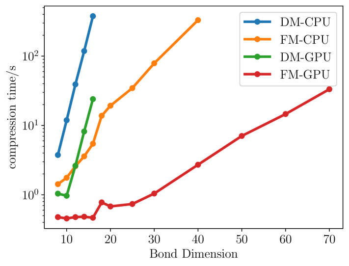
Figure 15: Compression time of multiplying three $N=20$ random tensor networks with the direct method (DM) and fitting method(FM). The direct method is not applicable for bond dimension $D>14$ due to memory constraints.

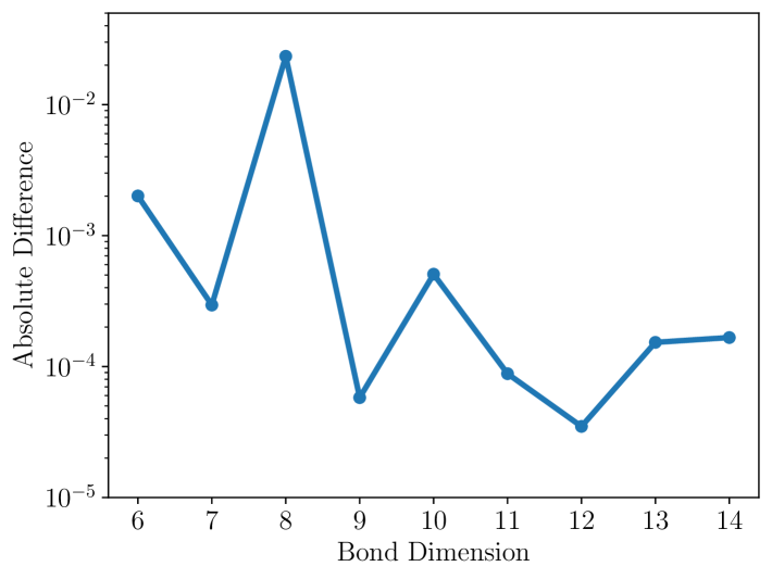
Figure 16: Absolute difference of $\mathrm{Tr}(HK_{a}\rho_{t=0.1}K_{a}^{\dagger})$ calculated using the direct method (DM) and the fitting method (FM) as the bond dimension $D$ increases.

Then, we numerically validate that the jump operator can be compressed into an MPO with relatively low bond dimension. To this end, we evaluate $\left\lVert K_{a}\left|\psi_{g}\right\rangle\right\rVert^{2}$ for the 1D-TFIM model with $J=1$ and $g=1.5$, using a fixed bond dimension $D=50$, with the coupling operator $X$ positioned at the center of the chain. We then investigate how $\left\lVert K_{a}\left|\psi_{g}\right\rangle\right\rVert^{2}$ scales with increasing system size $N$. Ideally, this quantity should remain small since $\left|\psi_{g}\right\rangle$ belongs to the kernel of the jump operator. Fig. 17 shows that $\left\lVert K_{a}\left|\psi_{g}\right\rangle\right\rVert^{2}$ remains approximately $10^{-3}$ as the system size grows. This result confirms that a bond dimension of $D=50$ can be sufficiently accurate for representing the ground state and the jump operators.

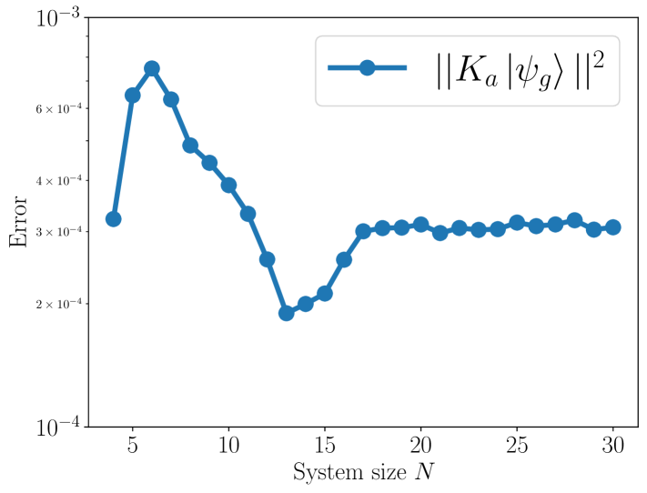
Figure 17: $\left\lVert K_{a}\left|\psi_{g}\right\rangle\right\rVert^{2}$ as a function of system size $N$ for the 1D-TFIM model with $a=\lfloor L/2\rfloor$. The bond dimension is set to $D=50$.

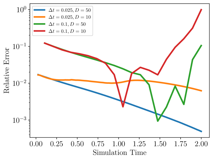
Figure 18: Relative error of energy with different time step sizes and bond dimensions for 1D TFIM model.

Finally, in Fig. 18, we demonstrate the reliability of the tensor network results by comparing simulations with different bond dimensions. We consider the bulk dissipation of an $N=10$ one-dimensional TFIM model using bond dimensions $D=10,50$ and a time step size of $\Delta t=0.025$. The relative error is computed using $D=75$ and $\Delta t=0.0125$ as the reference (see Fig. 18). For small simulation times, the dominant source of error is the time discretization. A large time step size may also lead to unstable behavior as the simulation time increases. Furthermore, as the system evolves towards a fixed point, the error is no longer primarily dictated by time discretization, and the bond dimension plays a more significant role.

Appendix F Proof of rapid ground state preparation of weakly interacting spin systems

In this section, we show the rapid ground state preparation for the perturbed Hamiltonian. First, we introduce the assumptions of the filter function $f$, which is similar to that in [18, Assumption 12]. Our analysis employs the Gevrey function, a subclass of smooth functions characterized by well-controlled decay of the Fourier coefficients. This characteristic plays a crucial role in the quadrature analysis.

Definition 7 (Gevrey function).

Let $\Omega\subseteq\mathbb{R}^{d}$ be a domain. A complex-valued $C^{\infty}$ function $h:\Omega\to\mathbb{C}$ is a Gevrey function of order $s\geq 0$, if there exist constants $C_{1},C_{2}>0$ such that for every $d$-tuple of nonnegative integers $\alpha=(\alpha_{1},\alpha_{2},\ldots,\alpha_{d})$,

$$\left\|\partial^{\alpha}h\right\|_{L^{\infty}(\Omega)}\leq C_{1}C^{|\alpha|}_{2}|\alpha|^{|\alpha|s}\,,$$ (86)

where $|\alpha|=\sum^{d}_{i=1}|\alpha_{i}|$. For fixed constants $C_{1},C_{2},s$, the set of Gevrey functions is denoted by $\mathcal{G}^{s}_{C_{1},C_{2}}(\Omega)$. Furthermore, $\mathcal{G}^{s}=\bigcup_{C_{1},C_{2}>0}\mathcal{G}^{s}_{C_{1},C_{2}}$.

We refer readers to [1, 31] for background on the Gevrey class. We also note that the use of Gevrey class functions is mainly for simplifying the discretization error analysis and not essential for the design of the Lindbladian.

Assumption 8 (Filter function in the frequency domain).

Assume $\hat{f}$ in the Fourier domain takes the form:

$$\hat{f}(\omega)=\hat{u}(\omega/8)\hat{v}(2\omega)\,.$$ (87)

Here, $\hat{u}$ is a positive function and belongs to Gevrey class $\mathcal{G}^{\alpha}_{A_{1,u},A_{2,u}}(\mathbb{R})$ for some $A_{1,u},A_{2,u}>0$ and $\alpha>1$, meaning that

$$\sup_{\omega\in\mathbb{R}}\left|\frac{\mathrm{d}^{n}}{\mathrm{d}\omega^{n}}\left(\hat{u}(\omega)\right)\right|\leq A_{1,u}A^{n}_{2,u}n^{n\alpha}$$

for any $n\in\mathbb{N}$. Also, $\mathrm{supp}(\hat{u})\subset[-1,1]$, $\hat{u}(\omega)=\Omega(1)$ when $\omega\in[-1/2,1/2]$, and $\hat{u}(-1/4)=1$. In addition, we assume $\hat{v}\in\mathcal{G}^{\alpha}_{A_{1,v},A_{2,v}}(\mathbb{R})$, $\left\|\frac{\mathrm{d}}{\mathrm{d}\omega}\hat{v}\right\|_{L^{1}}=\mathcal{O}(1)$, $\mathrm{supp}(\hat{v})\subset(-\infty,0]$, and $\hat{v}(-4)=1$.

Compared to [18, Assumption 12], the above assumption sets $\Delta=1/2$ and $S_{\omega}=4$, which is sufficient to ensure (93). First, setting $\Delta=1/2$ is adequate for our analysis since the spectral gap of $H_{0}$ is one, implying that the spectral gap of $H_{\varepsilon}$ remains greater than $1/2$ when $\varepsilon$ is sufficiently small. Second, choosing $S_{\omega}=4$ is sufficient because the coupling operator $A_{i}=X_{i}$ modifies the energy of $H_{0}$ by at most one, ensuring that the energy decay of $H_{\varepsilon}$ can also be bounded by 4 when $\varepsilon$ is sufficiently small.

Now, we are ready to present the rigorous version of Theorem 2:

Theorem 9 (Rigorous version of Theorem 2).

Assume $H$ is a $(r_{0},l)$-local Hamiltonian that takes the form of (34), choose the coupling operators $\{A_{a}\}=\{X_{i}\}_{i\in\Lambda}$, and the filter function $f$ satisfies Assumption 8. There exists a constant $\varepsilon^{*}$ only depends on $k,l,D$ such that when $\varepsilon<\varepsilon^{*}$, we have

$$\left\|\exp(\mathcal{L}t)\rho-\left|\psi_{0}\right\rangle\left\langle\psi_{0}\right|\right\|_{1}\leq\eta,\quad\forall t=\Omega(\log(N/\eta))\,,\ \rho$$

where $N=(L+1)^{D}$ is the system size. Here, $\varepsilon^{*}=\widetilde{\mathcal{O}}\left(\left(r_{0}l\right)^{-\Theta(D)}\right)$.

Following the argument in Section VII, to prove Theorem 9, it suffices to prove the following proposition. We will prove this proposition after giving the proof of Theorem 9.

Proposition 10.

Under the conditions of Theorem 9, for any observable $O$ such that $\|O\|\leq 1$, we have

$${\left|\kern-1.07639pt\left|\kern-1.07639pt\left|O(t)\right|\kern-1.07639pt\right|\kern-1.07639pt\right|}\leq{\left|\kern-1.07639pt\left|\kern-1.07639pt\left|O(0)\right|\kern-1.07639pt\right|\kern-1.07639pt\right|}\exp(-t/4).$$ (88)

Proof of Theorem 9.

Using the relation between the $1$-norm and the trace with observables,

$$\left\|\rho(t)-\sigma\right\|_{1}=\sup_{\|O\|\leq 1}\mathrm{Tr}\left(O\left(\rho(t)-\sigma\right)\right)\leq\sup_{\|O\|\leq 1}\left\|O(t)-\mathrm{Tr}(O(t))/2^{N}\right\|\left\|\rho(0)-\sigma\right\|_{1}\,.$$ (89)

We then notice

$$O(t)-\mathrm{Tr}(O(t))/2^{N}=\delta_{1}(O(t))+\sum^{N}_{i=2}\delta_{i}\circ\left(\frac{I_{\{1,\cdots,i-1\}}}{2^{i-1}}\otimes\mathrm{Tr}_{\{1,\cdots,i-1\}}(O(t))\right)\,.$$

Thus, we have

$$\left\|O(t)-\mathrm{Tr}(O(t))/2^{N}\right\|$$

$$\leq \left\|\delta_{1}(O(t))\right\|+\sum^{N}_{i=2}\left\|\delta_{i}\circ\left(\frac{I_{\{1,\cdots,i-1\}}}{2^{i-1}}\otimes\mathrm{Tr}_{\{1,\cdots,i-1\}}(O(t))\right)\right\|$$

$$= \left\|\delta_{1}(O(t))\right\|+\sum^{N}_{i=2}\left\|\left(\frac{I_{\{1,\cdots,i-1\}}}{2^{i-1}}\otimes\mathrm{Tr}_{\{1,\cdots,i-1\}}\right)\circ\delta_{i}(O(t))\right\|$$

$$\leq \sum^{N}_{i=1}\left\|\delta_{i}(O(t))\right\|\leq\sum^{N}_{i=1}\left\|\delta_{i}\circ P_{i}(O(t))\right\|+\left\|\delta_{i}\circ Q_{i}(O(t))\right\|={\left|\kern-1.07639pt\left|\kern-1.07639pt\left|O(t)\right|\kern-1.07639pt\right|\kern-1.07639pt\right|}\,.$$

This provides a proof of (40). Next, according to Proposition 10 and $\left\|\rho-\left|\psi_{0}\right\rangle\left\langle\psi_{0}\right|\right\|_{1}\leq 2N$, we have

$$\left\|\exp(\mathcal{L}t)\rho-\left|\psi_{0}\right\rangle\left\langle\psi_{0}\right|\right\|_{1}\leq 2N{\left|\kern-1.07639pt\left|\kern-1.07639pt\left|O(0)\right|\kern-1.07639pt\right|\kern-1.07639pt\right|}\exp(-t/4)\leq 8N^{2}\exp(-t/4)\,,$$

where we use ${\left|\kern-1.07639pt\left|\kern-1.07639pt\left|O(0)\right|\kern-1.07639pt\right|\kern-1.07639pt\right|}\leq 4N$ in the last inequality. This concludes the proof. ∎

In the following part of the section, we focus on the proof of Proposition 10. First, for simplicity, in the following part, we define

$$H_{\varepsilon}=-\sum_{i}Z_{i}+\varepsilon\sum_{j}h_{j}\,.$$ (90)

The jump operator is

$$K_{j,\varepsilon}=\int^{\infty}_{-\infty}f(t)\exp(iH_{\varepsilon}t)A_{j}\exp(-iH_{\varepsilon}t)\mathrm{d}t=\int^{\infty}_{-\infty}f(t)\exp(iH_{\varepsilon}t)X_{j}\exp(-iH_{\varepsilon}t)\mathrm{d}t\,,$$ (91)

and the corresponding dissipative term in the Lindbladian is

$$\mathcal{L}_{j,\varepsilon}(\rho)=K_{j,\varepsilon}\rho K^{\dagger}_{j,\varepsilon}-\frac{1}{2}\left\{K^{\dagger}_{j,\varepsilon}K_{j,\varepsilon},\rho\right\}\,.$$ (92)

When $\varepsilon=0$,

$$K_{j,0}=\int^{\infty}_{-\infty}f(t)\exp(iH_{0}t)X_{j}\exp(-iH_{0}t)\mathrm{d}t=\hat{f}(-2)\left|0_{j}\right\rangle\left\langle 1_{j}\right|=\left|0_{j}\right\rangle\left\langle 1_{j}\right|\,.$$ (93)

We start with the evolution of the observable $P_{i}(O(t))$:

$$\partial_{t}P_{i}(O(t))=P_{i}\left(\mathcal{L}^{\dagger}_{i,\varepsilon}(O(t))\right)+P_{i}\left(\sum_{j\neq i}\mathcal{L}^{\dagger}_{j,\varepsilon}(O(t))\right)$$

which implies

$$\partial_{t}\delta_{i}\circ P_{i}(O(t))=\delta_{i}\circ P_{i}\left(\mathcal{L}^{\dagger}_{i,\varepsilon}(O(t))\right)+\delta_{i}\circ P_{i}\left(\sum_{j\neq i}\mathcal{L}^{\dagger}_{j,\varepsilon}(O(t))\right)$$

$$= \delta_{i}\circ P_{i}\left(\mathcal{L}^{\dagger}_{i,0}(O(t))\right)+\delta_{i}\circ P_{i}\left(\mathcal{L}^{\dagger}_{i,\varepsilon}(O(t))-\mathcal{L}^{\dagger}_{i,0}(O(t))\right)+\sum_{j\neq i}\mathcal{L}^{\dagger}_{j,\varepsilon}\left(\delta_{i}\circ P_{i}\left(O(t)\right)\right)+\left[\delta_{i}\circ P_{i},\sum_{j\neq i}\mathcal{L}^{\dagger}_{j,\varepsilon}\right]\left(O(t)\right)$$

$$= \underbrace{-\delta_{i}\circ P_{i}(O(t))}_{\text{decaying part}}+\underbrace{\sum_{j\neq i}\mathcal{L}^{\dagger}_{j,\varepsilon}\left(\delta_{i}\circ P_{i}\left(O(t)\right)\right)}_{\text{contractive part}}+\delta_{i}\circ P_{i}\left(\mathcal{L}^{\dagger}_{i,\varepsilon}(O(t))-\mathcal{L}^{\dagger}_{i,0}(O(t))\right)+\left[\delta_{i}\circ P_{i},\sum_{j\neq i}\mathcal{L}^{\dagger}_{j,\varepsilon}\right]\left(O(t)\right)\,.$$

Here, the second term is contractive in the sense that $\left\|\exp\left(\sum_{j\neq i}\mathcal{L}^{\dagger}_{j,\varepsilon}t\right)\right\|_{\infty\to\infty}\leq 1$ for any $t>0$, which ensures that the perturbation error does not grow exponentially with time $t$. In the last equality, we use the fact that $\delta_{i}\circ P_{i}\left(\mathcal{L}^{\dagger}_{i,0}(O(t))\right)=-\delta_{i}\circ P_{i}(O(t))$ by direct calculation. Following the similar calculations in [57, Appendix A. Section I (A6-A8)], we obtain

$$\left\|\delta_{i}\circ P_{i}(O(t))\right\|$$ (94)

$$\leq\exp(-t)\left\|\delta_{i}\circ P_{i}(O)\right\|+\int^{t}_{0}\exp(s-t)\left\|\delta_{i}\circ P_{i}\left(\mathcal{L}^{\dagger}_{i,\varepsilon}(O(s))-\mathcal{L}^{\dagger}_{i,0}(O(s))\right)+\left[\delta_{i}\circ P_{i},\sum_{j\neq i}\mathcal{L}^{\dagger}_{j,\varepsilon}\right]\left(O(s)\right)\right\|_{\infty}\mathrm{d}s$$

Similar to the above calculation, for $Q_{i}(O(t))$, we also have

$$\partial_{t}\delta_{i}\circ Q_{i}(O(t))=\delta_{i}\circ Q_{i}\left(\mathcal{L}^{\dagger}_{i,\varepsilon}(O(t))\right)+\delta_{i}\circ Q_{i}\left(\sum_{j\neq i}\mathcal{L}^{\dagger}_{j,\varepsilon}(O(t))\right)$$

$$= \delta_{i}\circ Q_{i}\left(\mathcal{L}^{\dagger}_{i,0}(O(t))\right)+\delta_{i}\circ Q_{i}\left(\mathcal{L}^{\dagger}_{i,\varepsilon}(O(t))-\mathcal{L}^{\dagger}_{i,0}(O(t))\right)+\sum_{j\neq i}\mathcal{L}^{\dagger}_{j,\varepsilon}\left(\delta_{i}\circ Q_{i}\left(O(t)\right)\right)+\left[\delta_{i}\circ Q_{i},\sum_{j\neq i}\mathcal{L}^{\dagger}_{j,\varepsilon}\right]\left(O(t)\right)$$

$$= \underbrace{-\frac{1}{2}\delta_{i}\left(Q_{i}(O(t))\right)}_{\text{decaying part}}+\underbrace{\sum_{j\neq i}\mathcal{L}^{\dagger}_{j,\varepsilon}\left(\delta_{i}\circ Q_{i}\left(O(t)\right)\right)}_{\text{contractive part}}+\delta_{i}\circ Q_{i}\left(\mathcal{L}^{\dagger}_{i,\varepsilon}(O(t))-\mathcal{L}^{\dagger}_{i,0}(O(t))\right)+\left[\delta_{i}\circ Q_{i},\sum_{j\neq i}\mathcal{L}^{\dagger}_{j,\varepsilon}\right]\left(O(t)\right)\,.$$

This implies

$$\left\|\delta_{i}\left(Q_{i}(O(t))\right)\right\|$$ (95)

$$\leq\exp(-t)\left\|\delta_{i}\left(Q_{i}(O)\right)\right\|+\int^{t}_{0}\exp(s-t)\left\|\delta_{i}\circ Q_{i}\left(\mathcal{L}^{\dagger}_{i,\varepsilon}(O(s))-\mathcal{L}^{\dagger}_{i,0}(O(s))\right)+\left[\delta_{i}\circ Q_{i},\sum_{j\neq i}\mathcal{L}^{\dagger}_{j,\varepsilon}\right]\left(O(s)\right)\right\|_{\infty}\mathrm{d}s\,.$$

Combining (94) and (95), we obtain

$$\left\|\delta_{i}\left(P_{i}(O(t))\right)\right\|+\left\|\delta_{i}\left(Q_{i}(O(t))\right)\right\|$$ (96)

$$\leq \exp(-t/2)\left(\left\|\delta_{i}\left(P_{i}(O)\right)\right\|+\left\|\delta_{i}\left(Q_{i}(O)\right)\right\|\right)$$

$$+\int^{t}_{0}\exp(s-t)\left\|\delta_{i}\circ P_{i}\left(\mathcal{L}^{\dagger}_{i,\varepsilon}(O(s))-\mathcal{L}^{\dagger}_{i,0}(O(s))\right)+\left[\delta_{i}\circ P_{i},\sum_{j\neq i}\mathcal{L}^{\dagger}_{j,\varepsilon}\right]\left(O(s)\right)\right\|_{\infty}\mathrm{d}s$$

$$+\int^{t}_{0}\exp(s-t)\left\|\delta_{i}\circ Q_{i}\left(\mathcal{L}^{\dagger}_{i,\varepsilon}(O(s))-\mathcal{L}^{\dagger}_{i,0}(O(s))\right)+\left[\delta_{i}\circ Q_{i},\sum_{j\neq i}\mathcal{L}^{\dagger}_{j,\varepsilon}\right]\left(O(s)\right)\right\|_{\infty}\mathrm{d}s.$$

To bound the last two terms in Eq. 96. We introduce a lemma to bound the second and third terms in (96). First, given lattice $i$ and radius $r>0$, we define $H^{(i,r)}_{\varepsilon}$ as the Hamiltonian that consists of the Hamiltonian terms of $H_{\varepsilon}$ on a ball of radius $r$ centered at lattice $i$. $K^{r}_{i,\varepsilon}$, $\mathcal{L}^{r}_{i,\varepsilon}$ are defined according to (91) and (92) with $H^{(i,r)}_{\varepsilon}$. Then we have the following lemma:

Lemma 11.

Under conditions of Theorem 9 and let $J=r_{0}^{D}l$, for any $r\geq 1$, we have

$$\left\|\mathcal{L}_{i,\varepsilon}^{r\dagger}-\mathcal{L}_{i,\varepsilon}^{r-1\dagger}\right\|_{\infty\rightarrow\infty}\leq\xi(r)=\mathcal{O}\left(\frac{1}{2^{r}}+\exp(-C_{2,f}(r/(4Je))^{1/\alpha}/2)\right),$$ (97)

$$\left\|\mathcal{L}_{i,\varepsilon}^{\dagger}-\mathcal{L}_{i,0}^{\dagger}\right\|_{\infty\rightarrow\infty}\leq\eta(\varepsilon)=\mathcal{O}\left(\varepsilon(J\log^{\alpha}(1/\varepsilon)+1)^{D}l\right)\,.$$

With Lemma 11, we are ready to provide the proof of Proposition 10.

Proof of Proposition 10.

The proof follows a similar strategy to that in [57, Appendix A. Section I]. We first claim that, there exists $\kappa^{c}_{i}$ and $\gamma^{c}_{i}$ such that

$$\left\|\left[\delta_{i}\circ P_{i},\mathcal{L}^{\dagger}_{j,\varepsilon}\right]\left(O\right)\right\|,\quad\left\|\left[\delta_{i}\circ Q_{i},\mathcal{L}^{\dagger}_{j,\varepsilon}\right]\left(O\right)\right\|\leq\sum_{k}\kappa^{k}_{i,j}\left(\|\delta_{k}\circ P_{k}(O)\|+\|\delta_{k}\circ Q_{k}(O)\|\right)$$ (98)

and

$$\left\|\delta_{i}\circ P_{i}\left(\mathcal{L}^{\dagger}_{i,\varepsilon}(O)-\mathcal{L}^{\dagger}_{i,0}(O)\right)\right\|,\left\|\delta_{i}\circ Q_{i}\left(\mathcal{L}^{\dagger}_{i,\varepsilon}(O)-\mathcal{L}^{\dagger}_{i,0}(O)\right)\right\|\leq\sum_{k}\gamma^{k}_{i}\left(\|\delta_{k}\circ P_{k}(O)\|+\|\delta_{k}\circ Q_{k}(O)\|\right)$$ (99)

with $\sum_{i,j\neq i}\kappa^{k}_{i,j}+\sum_{i}\gamma^{k}_{i}$ is smaller than a constant that is independent of the system size.

Denote by $d(i,j)$ the Manhattan distance between sites $i,j\in\Lambda$ and $\Gamma(r_{0})=\sum_{r\geq r_{0}}\xi(r)=\mathcal{O}\left(2^{-r}\right)$ when $r_{0}\geq 4kl$. We first show (98) and calculate $\kappa$. Following the calculations in [57, Appendix B] and letting $B_{j}(r)=\{j|d(i,j)\leq r\}$, we get

$$\left\|\left[\delta_{i}\circ P_{i},\mathcal{L}_{j,\varepsilon}^{\dagger}\right](O)\right\|_{\infty}=\left\|\left[\delta_{i}\circ P_{i},\left(\mathcal{L}_{j,\varepsilon}^{\dagger}-\mathcal{L}_{j,\varepsilon}^{d(i,j)\dagger}\right)\right](O)\right\|_{\infty}$$ (100)

$$\leq \left\|\mathcal{L}_{j,\varepsilon}^{\dagger}-\mathcal{L}_{j,\varepsilon}^{d(i,j)\dagger}\right\|_{\infty\rightarrow\infty}\left\|\delta_{i}\circ P_{i}(O))\right\|_{\infty}+2\left\|\left(\mathcal{L}_{j,\varepsilon}^{\dagger}-\mathcal{L}_{j,\varepsilon}^{d(i,j)\dagger}\right)(O)\right\|_{\infty}$$

$$\leq \sum_{r>d(i,j)}\zeta(r)\left\|\delta_{i}\circ P_{i}(O))\right\|_{\infty}+2\sum_{r>d(i,j)}\left\|\left((\mathcal{L}^{r}_{j,\varepsilon})^{\dagger}-(\mathcal{L}^{r-1}_{j,\varepsilon})^{\dagger}\right)\delta_{B_{j}(r)}(O)\right\|_{\infty}$$

$$\leq \Gamma(d(i,j))\left\|\delta_{i}\circ P_{i}(O))\right\|_{\infty}+2\sum_{r>d(i,j)}\zeta(r)\sum_{d(j,k)\leq r}(\left\|\delta_{k}\circ P_{k}(O))\right\|_{\infty}+\left\|\delta_{k}\circ Q_{k}(O))\right\|_{\infty})$$

$$= \Gamma(d(i,j))\left\|\delta_{i}\circ P_{i}(O))\right\|_{\infty}+2\sum_{k}(\left\|\delta_{k}\circ P_{k}(O))\right\|_{\infty}+\left\|\delta_{k}\circ Q_{k}(O))\right\|_{\infty})\Gamma(\max(d(i,j),d(j,k))).$$

Let $r_{0}>0$, to be determined later. For $d(i,j)\geq r_{0}$, we have

$$\kappa^{k}_{i,j}=\left\{\begin{aligned} &\Gamma(d(i,j)),\quad k=i\\ &2\Gamma(\max(d(i,j),d(j,k))),\quad k\neq i.\end{aligned}\right.$$ (101)

For $d(i,j)<r_{0}$, we can bound the commutator as follows:

$$\left\|\left[\delta_{i}\circ P_{i},\mathcal{L}_{j,\varepsilon}^{\dagger}\right](O)\right\|_{\infty}\leq\left\|\left[\delta_{i}\circ P_{i},\left(\mathcal{L}_{j,\varepsilon}^{\dagger}-\mathcal{L}_{j,\varepsilon}^{r_{0},\dagger}\right)\right](O)\right\|_{\infty}+\left\|\left[\delta_{i}\circ P_{i},\left(\mathcal{L}_{j,\varepsilon}^{r_{0},\dagger}-\mathcal{L}_{j,0}^{r_{0},\dagger}\right)\right](O)\right\|_{\infty}$$ (102)

$$\quad\leq \left(\eta(\varepsilon)+\Gamma\left(r_{0}\right)\right)\left\|\delta_{i}\circ P_{i}(O))\right\|_{\infty}+2\sum_{r>r_{0}}\zeta(r)\sum_{d(k,j)\leq r}(\left\|\delta_{k}\circ P_{k}(O))\right\|_{\infty}+\left\|\delta_{k}\circ Q_{k}(O))\right\|_{\infty})$$

$$+2\eta(\varepsilon)\sum_{d(k,j)\leq r_{0}}(\left\|\delta_{k}\circ P_{k}(O))\right\|_{\infty}+\left\|\delta_{k}\circ Q_{k}(O))\right\|_{\infty})$$

$$\quad\leq \left(\eta(\varepsilon)+\Gamma\left(r_{0}\right)\right)\left\|\delta_{i}\circ P_{i}(O))\right\|_{\infty}+2\sum_{c}\Gamma\left(\max\left(r_{0},d(k,j)\right)\right)(\left\|\delta_{k}\circ P_{k}(O))\right\|_{\infty}+\left\|\delta_{k}\circ Q_{k}(O))\right\|_{\infty})$$

$$+2\eta(\varepsilon)\sum_{d(k,j)\leq r_{0}}(\left\|\delta_{k}\circ P_{k}(O))\right\|_{\infty}+\left\|\delta_{k}\circ Q_{k}(O))\right\|_{\infty})\,.$$

Therefore, for $d(i,j)<r_{0}$ we have

$$\kappa^{k}_{i,j}=\left\{\begin{aligned} &3\eta(\varepsilon)+3\Gamma\left(r_{0}\right),\quad d(k,j)\leq r_{0}\\ &2\Gamma\left(d(k,j)\right),\quad d(k,j)>r_{0}\end{aligned}\right.\,.$$ (103)

Similarly, we can also show (99) and calculate $\gamma$. We have

$$\begin{aligned} \left\|\delta_{i}\circ P_{i}\left(\mathcal{L}^{\dagger}_{i,\varepsilon}-\mathcal{L}^{\dagger}_{i,0}\right)(O)\right\|_{\infty}&\leq\left\|\delta_{i}\circ P_{i}\left(\mathcal{L}^{\dagger}_{i,\varepsilon}-\mathcal{L}^{r_{0},\dagger}_{i,\varepsilon}\right)(O)\right\|_{\infty}+\left\|\delta_{i}\circ P_{i}\left(\mathcal{L}^{r_{0},\dagger}_{i,\varepsilon}-\mathcal{L}^{\dagger}_{i,0}\right)(O)\right\|_{\infty}\\ &\leq\eta(\varepsilon)\sum_{d(i,k)\leq r_{0}}\left\|\delta_{k}\circ P_{k}(O))\right\|_{\infty}+2\sum_{r\geq r_{0}}\zeta(r)\sum_{d(i,k)\leq r}(\left\|\delta_{k}\circ P_{k}(O))\right\|_{\infty}+\left\|\delta_{k}\circ Q_{k}(O))\right\|_{\infty})\\ &\leq\eta(\varepsilon)\sum_{d(i,k)\leq r_{0}}\left\|\delta_{k}\circ P_{k}(O))\right\|_{\infty}\\ &+2\sum_{j}\Gamma\left(\max\left(r_{0},d(i,k)\right)\right)(\left\|\delta_{k}\circ P_{k}(O))\right\|_{\infty}+\left\|\delta_{k}\circ Q_{k}(O))\right\|_{\infty}).\end{aligned}\,.$$ (104)

This implies

$$\gamma^{k}_{i}=\left\{\begin{aligned} &\eta(\varepsilon)+2\Gamma\left(r_{0}\right),\quad d(i,k)\leq r_{0}\\ &2\Gamma\left(d(i,k)\right),\quad d(i,k)>r_{0}.\end{aligned}\right.$$ (105)

Similar to the calculations in [57, Appendix A.2], we get

$$\kappa=\sum_{i,j\neq i}\kappa_{i,j}^{k}+\sum_{i}\gamma_{i}^{k}\leq 4\left(2r_{0}+1\right)^{2D}\eta(\varepsilon)+20\sum_{m^{\prime}\geq r_{0}}\sum_{m\geq m^{\prime}}(2m+1)^{2D+1}\Gamma(m)\,.$$ (106)

Choosing $r_{0}=\Theta(\max\{J,D^{2}\})$ sufficiently large so that the second term is smaller than $1/8$, we then set $\varepsilon$ small enough so that

$$\varepsilon=\mathcal{O}\left((2r_{0}+1)^{-2D}(J\log^{\alpha}(1/\varepsilon)+1)^{-D}l^{-1}\right)\,,$$

we have $\kappa<1/4$.

Plugging (98) and (99) into (96), we have

$$\left\|\delta_{i}\left(P_{i}(O(t))\right)\right\|+\left\|\delta_{i}\left(Q_{i}(O(t))\right)\right\|$$ (107)

$$\leq\exp(-t/2)(\left\|\delta_{i}\left(P_{i}(O)\right)\right\|+\left\|\delta_{i}\left(Q_{i}(O)\right)\right\|)$$

$$+\kappa\int^{t}_{0}\exp(s-t)(\left\|\delta_{i}\left(P_{i}(O(s))\right)\right\|+\left\|\delta_{i}\left(Q_{i}(O(s))\right)\right\|)\mathrm{d}s$$

Because $\kappa<1/4$, we can bound $\left\|\delta_{i}\left(P_{i}(O(t))\right)\right\|+\left\|\delta_{i}\left(Q_{i}(O(t))\right)\right\|$:

$${\left|\kern-1.07639pt\left|\kern-1.07639pt\left|O(t)\right|\kern-1.07639pt\right|\kern-1.07639pt\right|}=\sum_{i}\left(\left\|\delta_{i}\left(P_{i}(O(t))\right)\right\|+\left\|\delta_{i}\left(Q_{i}(O(t))\right)\right\|\right)\leq e^{-t/4}\sum_{i}\left(\left\|\delta_{i}\left(P_{i}(O)\right)\right\|+\left\|\delta_{i}\left(Q_{i}(O)\right)\right\|\right)$$ (108)

This concludes the proof. ∎

Finally, we provide the proof of Lemma 11.

Proof of Lemma 11.

According to [18, Lemma 16] with $\Delta=1/2$ and $S_{\omega}=4$ (see the detailed explanation about this choice under Assumption 8), the filter function in the time domain satisfies $|f(s)|=\mathcal{O}(C_{1,f}\exp(-C_{2,f}|s|^{1/\alpha})$, where $C_{1,f},C_{2,f}$ are constants that only depend on $A_{1,u},A_{2,u},A_{1,v},A_{2,v}$ in Assumption 8. This directly implies

$$\|(|s|+1)f(s)\|_{L^{1}}\leq C\,.$$ (109)

where $C$ only depends on $A_{1,u},A_{2,u},A_{1,v},A_{2,v}$, and $\alpha$.

We first show the bound of $\left\|\mathcal{L}^{\dagger}_{i,\varepsilon}-\mathcal{L}^{\dagger}_{i,0}\right\|_{\infty\rightarrow\infty}$. Note

$$\left\|\mathcal{L}^{\dagger}_{i,\varepsilon}-\mathcal{L}^{\dagger}_{i,0}\right\|_{\infty\rightarrow\infty}\leq 2\left(\left\|K_{j,\varepsilon}\right\|+\left\|K_{j,0}\right\|_{\infty}\right)\left\|K_{j,\varepsilon}-K_{j,0}\right\|_{\infty}\leq 4\|f(t)\|_{L^{1}}\left\|K_{j,\varepsilon}-K_{j,0}\right\|\,.$$ (110)

Let $J=r_{0}^{D}l$. Next,

$$\left\|K_{j,\varepsilon}-K_{j,0}\right\|_{\infty}=\left\|\int^{\infty}_{-\infty}f(t)\left[\exp(iH_{\varepsilon}t)X_{j}\exp(-iH_{\varepsilon}t)-\exp(iH_{0}t)X_{j}\exp(-iH_{0}t)\right]\mathrm{d}t\right\|_{\infty}$$

$$= \left\|\int^{\infty}_{-\infty}f(t)\underbrace{\left[\exp(iH_{\varepsilon}t)X_{j}\exp(-iH_{\varepsilon}t)-\exp(iH^{(j,r)}_{\varepsilon}t)X_{j}\exp(-iH^{(j,r)}_{\varepsilon}t)\right]}_{\left\|\cdot\right\|\leq\|X_{j}\|_{\infty}\min\left\{\frac{(2J|t|)^{r}}{r!},2\right\}}\mathrm{d}t\right.$$

$$+\int^{\infty}_{-\infty}f(t)\left[\exp(iH^{(j,r)}_{\varepsilon}t)X_{j}\exp(-iH^{(j,r)}_{\varepsilon}t)-\exp(iH^{(j,r)}_{0}t)X_{j}\exp(-iH^{(j,r)}_{0}t)\right]\mathrm{d}t$$

$$\left.+\int^{\infty}_{-\infty}f(t)\underbrace{\left[\exp(iH^{(j,r)}_{0}t)X_{j}\exp(-iH^{(j,r)}_{0}t)-\exp(iH_{0}t)X_{j}\exp(-iH_{0}t)\right]}_{=0\ \forall r>1}\mathrm{d}t\right\|_{\infty}$$

$$\leq \int^{\infty}_{-\infty}f(t)\left(\min\left\{\frac{(2J|t|)^{r}}{r!},2\right\}+\left\|\exp(iH^{(j,r)}_{\varepsilon}t)-\exp(iH^{(j,r)}_{0}t)\right\|\right)\mathrm{d}t$$

$$\leq \int^{\infty}_{-\infty}f(t)\left(\min\left\{\frac{(2J|t|)^{r}}{r!},2\right\}+\left\|H^{(j,r)}_{\varepsilon}-H^{(j,r)}_{0}\right\||t|\right)\mathrm{d}t$$

$$\leq \int^{\infty}_{-\infty}f(t)\left(\min\left\{\frac{(2J|t|)^{r}}{r!},2\right\}+\varepsilon(r+1)^{D}l|t|\right)\mathrm{d}t$$

$$= \mathcal{O}\left(\int_{|t|\leq\frac{r}{4Je}}\frac{(2J)^{r}|t|^{r}}{r!}|f(t)|\mathrm{d}t+\int_{|t|>\frac{r}{4Je}}|f(t)|\mathrm{d}t+\varepsilon(r+1)^{D}l\right)$$

$$= \mathcal{O}\left(\int_{|t|\leq\frac{r}{4Je}}\frac{(2J)^{r}|t|^{r-1}}{r!}\mathrm{d}t+\int_{|t|>\frac{r}{4Je}}\exp(-C_{2,f}|t|^{1/\alpha})\mathrm{d}t+\varepsilon(r+1)^{D}l\right)$$

$$= \mathcal{O}\left(\frac{1}{2^{r}}+\int_{|t|>\frac{r}{4Je}}\exp(-C_{2,f}|t|^{1/\alpha})\mathrm{d}t+\varepsilon(r+1)^{D}l\right)$$

In the last third equality, we use (109).

Next, to bound the second term, we let $C_{\alpha,C_{2,f}}$ be the constant that depends on $\alpha$ and $C_{2,f}$ such that $\alpha\left|u^{\alpha-1}\right|<\exp(C_{2,f}u/2)$ for any $|u|>C_{\alpha,C_{2,f}}$. When $r>4JeC_{\alpha,C_{2,f}}^{\alpha}$,

$$\int_{|t|>\frac{r}{4Je}}\exp(-C_{2,f}|t|^{1/\alpha})\mathrm{d}t$$

$$= 2\int_{u>(\frac{r}{4Je})^{1/\alpha}}\alpha u^{\alpha-1}\exp(-C_{2,f}|u|)\mathrm{d}u$$

$$\leq 2\int_{u>(\frac{r}{4Je})^{1/\alpha}}\exp(-C_{2,f}|u|/2)\mathrm{d}u=\frac{4}{C_{2,f}}\exp\left(-C_{2,f}\left(\frac{r}{4Je}\right)^{1/\alpha}/2\right)$$

where we let $u=t^{1/\alpha}$ in the first equality. In the inequality, we use $\alpha\left|u\right|^{\alpha-1}<\exp(C_{2,f}u/2)$ for $|u|>C_{\alpha,C_{2,f}}$.

In conclusion, we can set $r=\Theta\left(\max\left\{J\log^{\alpha}(1/\varepsilon),JC_{\alpha,C_{2,f}}^{\alpha}\right\}\right)$ to obtain

$$\left\|K_{j,\varepsilon}-K_{j,0}\right\|_{\infty}$$

$$= \mathcal{O}\left(\frac{1}{2^{r}}+\int_{|t|>\frac{r}{4Je}}\exp(-C_{2,f}|s|^{1/\alpha})\mathrm{d}t+\varepsilon(r+1)^{D}l\right)$$

$$= \mathcal{O}\left(\frac{1}{2^{r}}+\exp(-C_{2,f}(r/(4Je))^{1/\alpha}/2)+\varepsilon(r+1)^{D}l\right)\,.$$

Plugging this into (110), we obtain

$$\eta(\varepsilon)=O\left(\varepsilon(J\log^{\alpha}(1/\varepsilon)+1)^{D}l\right)\,.$$ (111)

Next we calculate the function $f(r)$

$$\left\|\mathcal{L}^{r,\dagger}_{i,\varepsilon}-\mathcal{L}^{r-1,\dagger}_{i,\varepsilon}\right\|_{\infty\rightarrow\infty}\leq 2\left(\left\|K^{r}_{j,\varepsilon}\right\|_{\infty}+\left\|K^{r-1}_{j,\varepsilon}\right\|_{\infty}\right)\left\|K^{r}_{j,\varepsilon}-K^{r-1}_{j,\varepsilon}\right\|_{\infty}\leq 4\|f\|_{L^{1}}\left\|K^{r}_{j,\varepsilon}-K_{j,\varepsilon}^{r-1}\right\|_{\infty}\,.$$

The term $\left\|K^{r}_{j,\varepsilon}-K_{j,\varepsilon}^{r-1}\right\|$ can be calculated using Lieb-Robinson bound:

$$\left\|K^{r}_{j,\varepsilon}-K^{r-1}_{j,\varepsilon}\right\|_{\infty} =\left\|\int^{\infty}_{-\infty}f(t)\left[\exp(iH_{\varepsilon}^{(j,r)}t)X_{j}\exp(-iH_{\varepsilon}^{(j,r)}t)-\exp(iH_{\varepsilon}^{(j,r-1)}t)X_{j}\exp(-iH_{\varepsilon}^{(j,r-1)}t)\right]\mathrm{d}t\right\|_{\infty}$$ (112)

$$\leq\int^{\infty}_{-\infty}f(t)\left\|\exp(iH_{\varepsilon}^{(j,r)}t)X_{j}\exp(-iH_{\varepsilon}^{(j,r)}t)-\exp(iH_{\varepsilon}^{(j,r-1)}t)X_{j}\exp(-iH_{\varepsilon}^{(j,r-1)}t)\right\|_{\infty}\mathrm{d}t$$

$$\leq\int^{\infty}_{-\infty}f(t)\min\left\{\frac{(2J|t|)^{r}}{r!},2\right\}\mathrm{d}t$$

$$=\mathcal{O}\left(\frac{1}{2^{r}}+\int_{|t|>\frac{r}{4Je}}\exp(-C_{2,f}|s|^{1/\alpha})\mathrm{d}t\right)\,.$$

As a result, we get

$$\xi(r)=\mathcal{O}\left(\frac{1}{2^{r}}+\exp(-C_{2,f}(r/(4Je))^{1/\alpha}/2)\right)\,.$$

This concludes the proof. ∎

Appendix G Proof of rapid ground state preparation of weakly interacting fermionic systems

We first present the rigorous version of Theorem 3 for weakly interacting fermionic systems.

Theorem 12 (Rigorous version of Theorem 3).

Consider a gapped fermionic Hamiltonian $H$ in the form of (41) defined on a $D$-dimensional lattice $\Lambda=[0,L]^{D}$, and $N=(L+1)^{D}$ is the system size. Let $\{A_{a}\}=\{c^{\dagger}_{i},c_{i}\}_{i\in\Lambda}$ be a set of coupling operators and $\{K_{a}\}$ be the corresponding jump operators defined via Eq. 3. Assume the following conditions hold:

• $M\succ\Delta$ for some $\Delta>0$.

• The filter functions $f$ is chosen properly to satisfy

  $$\hat{f}(\nu)=1,\quad\forall\nu\in[-\|M\|,-\Delta],\quad\text{and}\quad\hat{f}(\nu)=0,\quad\forall\nu>0\,,$$ (113)

  $$\max\{|f(t)|\}\leq C_{1}\|M\|\exp(-C_{2}|t/\Delta|^{1/\alpha})\,,$$

  where $C_{1},C_{2},\alpha>0$ are constants independent of $N$.

Consider the Lindblad dynamics in Eq. 33. Then there exists a constant $\varepsilon^{*}$ independent of $L$ and $N$ such that when $\varepsilon<\varepsilon^{*}$, we have

$$\tau_{\operatorname{mix}}(\eta)=\Theta(\log(N/\eta))\,,$$ (114)

where $\tau_{\operatorname{mix}}(\eta)$ is defined in (4). Here, $\varepsilon^{*}=\widetilde{\mathcal{O}}\left(\left(\left(\max_{i,j}|M_{i,j}|\right)r_{0}l/\Delta\right)^{-\Theta(D)}\|M\|^{-1}\right)$.

The existence of $f$ follows from [1]. According to the proof of [1, Corollary 2.8], there exists a function $g$ belongs to $\mathcal{G}^{\alpha}_{A_{1,u},A_{2,u}}(\mathbb{R})$ for some $A_{1,u},A_{2,u}>0$ such that $g(x)=1$ when $x\geq 1$, $0\leq g(x)\leq 1$ when $x\in[1/2,1]$, and $g(x)=0$ when $x\leq 1/2$. According to [18, Lemmas 14, 15], $\hat{f}(\nu)=g(-\nu/\Delta)g((\|M\|+1+\nu)/\Delta)$ satisfies the condition (113).

Before proceeding, we introduce a more explicit definition of the fermionic partial trace that does not depend on the convention of commuting states past operators. This definition is equivalent to that in  Eq. 45 for operators of even parity.

For any observable $O$, we express it in fermionic form with increasing order, meaning

$$O=\sum_{\begin{subarray}{c}\mathbf{a},\mathbf{b}\end{subarray}}g_{\mathbf{a},\mathbf{b}}(c^{\dagger}_{1})^{a_{1}}(c_{1})^{b_{1}}\cdots(c^{\dagger}_{n})^{a_{n}}(c_{n})^{b_{n}}\,.$$ (115)

where $\mathbf{a},\mathbf{b}\in\{0,1\}^{N}$ and $c_{i},c^{\dagger}_{i}$ are creation and annihilation operators on $i$-th site.

We will only consider operators of even parity. Define the fermionic partial trace as

$$\mathrm{Tr}^{f}_{j}\left(O\right)= \sum_{\begin{subarray}{c}\sum_{i}a_{i}+b_{i}\,\mathrm{mod}\,2=0\\ a_{j}=b_{j}=1\end{subarray}}g_{\mathbf{a},\mathbf{b}}(c^{\dagger}_{1})^{a_{1}}(c_{1})^{b_{1}}\cdots(c^{\dagger}_{j}c_{j}+c_{j}c^{\dagger}_{j})\cdots(c^{\dagger}_{n})^{a_{n}}(c_{n})^{b_{n}}$$ (116)

$$+ 2\sum_{\begin{subarray}{c}\sum_{i}a_{i}+b_{i}\,\mathrm{mod}\,2=0\\ a_{j}=b_{j}=0\end{subarray}}g_{\mathbf{a},\mathbf{b}}(c^{\dagger}_{1})^{a_{1}}(c_{1})^{b_{1}}\cdots(c^{\dagger}_{j}c_{j}+c_{j}c^{\dagger}_{j})\cdots(c^{\dagger}_{n})^{a_{n}}(c_{n})^{b_{n}}.$$

Here we note $c^{\dagger}_{j}c_{j}+c_{j}c^{\dagger}_{j}=1=(c^{\dagger}_{j})^{0}(c_{j})^{0}$, and partial trace does not change the parity of the operator.

Using the notational convention $\left|1_{j}\right\rangle=c^{\dagger}_{j}\left|\mathrm{vac}\right\rangle$, $c_{k}\left|1_{j}\right\rangle=-\left|1_{j}\right\rangle c_{k}$ and $c^{\dagger}_{k}\left|1_{j}\right\rangle=-\left|1_{j}\right\rangle c^{\dagger}_{k}$, we may check that

$$\mathrm{Tr}^{f}_{j}(O)=\sum_{\begin{subarray}{c}\mathbf{a},\mathbf{b}\end{subarray}}g_{\mathbf{a},\mathbf{b}}(c^{\dagger}_{1})^{a_{1}}(c_{1})^{b_{1}}\cdots\left(\left\langle 0_{j}\right|(c^{\dagger}_{j})^{a_{j}}(c_{j})^{b_{j}}\left|0_{j}\right\rangle+(-1)^{\sum_{i\neq j}a_{i}+b_{i}}\left\langle 1_{j}\right|(c^{\dagger}_{j})^{a_{j}}(c_{j})^{b_{j}}\left|1_{j}\right\rangle\right)\cdots(c^{\dagger}_{n})^{a_{n}}(c_{n})^{b_{n}}.$$ (117)

When $O$ has even parity, $(-1)^{\sum_{i\neq j}a_{i}+b_{i}}=1$ for all non-vanishing terms. This proves the equivalence between the partial trace defined in Eq. 116 and (45).

Next, to express the formulas for $P_{i}$ and $Q_{i}$, we rewrite $O$ as $O=\sum_{a_{i},b_{i}=0}^{1}\left(c^{\dagger}_{i}\right)^{a_{i}}\left(c_{i}\right)^{b_{i}}\otimes_{F}O^{i}_{a,b}$, where $\otimes_{F}$ denotes the fermionic tensor product, which follows the increasing order convention as in (115). Specifically, $\{O^{i}_{a,b}\}$ are defined in the following

$$c^{\dagger}_{i}c_{i}\otimes_{F}O^{i}_{1,1}=c^{\dagger}_{i}c_{i}Oc^{\dagger}_{i}c_{i},$$ (118)

$$(c^{\dagger}_{i})^{0}(c_{i})^{0}\otimes_{F}O^{i}_{0,0}=c_{i}c^{\dagger}_{i}Oc_{i}c^{\dagger}_{i}+c^{\dagger}_{i}Oc_{i}$$

$$c_{i}\otimes_{F}O^{i}_{0,1}=c_{i}c^{\dagger}_{i}Oc^{\dagger}_{i}c_{i},\ c^{\dagger}_{i}\otimes_{F}O^{i}_{1,0}=c^{\dagger}_{i}c_{i}Oc_{i}c^{\dagger}_{i}\,.$$

Then we have two projection operators can be expressed as follows:

$$P_{i}(O)=\sum_{a_{i}=b_{i}}\left(c^{\dagger}_{i}\right)^{a_{i}}\left(c_{i}\right)^{b_{i}}\otimes_{F}O^{i}_{a,b}\,,$$ (119)

and

$$Q_{i}(O)=\sum_{a_{i}\neq b_{i}}\left(c^{\dagger}_{i}\right)^{a_{i}}\left(c_{i}\right)^{b_{i}}\otimes_{F}O^{i}_{a,b}\,.$$ (120)

The proof of Theorem 12 follows a similar strategy to that of Theorem 2 illustrated in Section VII. We first handle the non-interacting case using the new fermionic oscillator norm in Section G.1. Then, in Section G.2, we extend the proof to the perturbative regime. The proof of properties of the fermionic partial trace and the fermionic local oscillation operator will be given in Section G.3.

G.1 Non-interacting case

In this section, we consider the non-interacting case with $\varepsilon=0$ and $H=H_{0}$. We first calculate $K_{i}$:

• When $A_{i}=c_{i}$,

  $$K_{i}= \int^{\infty}_{-\infty}f(t)\exp(iH_{0}t)c_{i}\exp(-iH_{0}t)\mathrm{d}t=\sum_{q}c_{q}\int^{\infty}_{-\infty}f(s)(e^{-iMs})_{iq}\mathrm{d}s$$

  $$= \sum_{q}c_{q}\left(\hat{f}(-M)\right)_{iq}=c_{i}\,.$$

  where we use $\hat{f}(-M)$ is an identity according to the conditions of $f$.

• When $A_{i}=c^{\dagger}_{i}$,

  $$K_{i}= \int^{\infty}_{-\infty}f(t)\exp(iH_{0}t)c^{\dagger}_{i}\exp(-iH_{0}t)\mathrm{d}t=\sum_{q}c^{\dagger}_{q}\int^{\infty}_{-\infty}f(s)(e^{-iMs})_{qi}\mathrm{d}s$$

  $$= \sum_{q}c^{\dagger}_{q}\left(\hat{f}(M)\right)_{qi}=0\,,$$

  where we use $\hat{f}(M)=0$ according to the conditions of $f$.

Thus, we have the Lindbladian dynamics:

$$\frac{\mathrm{d}\rho}{\mathrm{d}t}=\mathcal{L}[\rho]=\sum_{i}\underbrace{c_{i}\rho c_{i}^{\dagger}-\frac{1}{2}\left\{c_{i}^{\dagger}c_{i},\rho\right\}}_{:=\mathcal{L}^{\dagger}_{i}(\rho)}\,.$$

Now, we first prove Theorem 12 for the simplest case $\varepsilon=0$.

Proof of Theorem 12 when $\varepsilon=0$.

Let $O=\sum^{1}_{a_{i},b_{i}=0}\left(c^{\dagger}_{i}\right)^{a_{i}}\left(c_{i}\right)^{b_{i}}\otimes_{F}O^{i}_{a,b}$, where $\otimes_{F}$ is the fermionic tensor product that follows the increasing order as in the form of (115). Here,

$$c^{\dagger}_{i}c_{i}\otimes_{F}O^{i}_{1,1}=c^{\dagger}_{i}c_{i}Oc^{\dagger}_{i}c_{i},\ c^{\dagger}_{i}\otimes_{F}O^{i}_{1,0}=c^{\dagger}_{i}c_{i}Oc_{i}c^{\dagger}_{i},\ c_{i}\otimes_{F}O^{i}_{0,1}=c_{i}c^{\dagger}_{i}Oc^{\dagger}_{i}c_{i},\ (c^{\dagger}_{i})^{0}(c_{i})^{0}\otimes_{F}O^{i}_{0,0}=c_{i}c^{\dagger}_{i}Oc_{i}c^{\dagger}_{i}+c^{\dagger}_{i}Oc_{i}\,.$$

We notice

$$c^{\dagger}_{i}Oc_{i}-\frac{1}{2}\left\{c^{\dagger}_{i}c_{i},O\right\}=-c^{\dagger}_{i}c_{i}\otimes_{F}O^{i}_{1,1}-\frac{1}{2}c_{i}\otimes_{F}O^{i}_{0,1}-\frac{1}{2}c^{\dagger}_{i}\otimes_{F}O^{i}_{1,0}\,.$$

Here, we did not generate parity sign in the first term because $O$ has even parity. This implies

$$\delta^{f}_{i}\left(c^{\dagger}_{i}Oc_{i}-\frac{1}{2}\left\{c^{\dagger}_{i}c_{i},O\right\}\right)=\frac{1}{2}(c_{i}c^{\dagger}_{i}-c^{\dagger}_{i}c_{i})\otimes_{F}O^{i}_{1,1}-\frac{1}{2}c_{i}\otimes_{F}O^{i}_{0,1}-\frac{1}{2}c^{\dagger}_{i}\otimes_{F}O^{i}_{1,0}$$

At the same time, we notice

$$\delta^{f}_{i}(O)=\frac{1}{2}(c^{\dagger}_{i}c_{i}-c_{i}c^{\dagger}_{i})\otimes_{F}O^{i}_{1,1}+c_{i}\otimes_{F}O^{i}_{0,1}+c^{\dagger}_{i}\otimes_{F}O^{i}_{1,0}\,.$$

According to the commuting property in Lemma 5, let

$$O_{1,i}=\sum_{a_{i}=b_{i}}\left(c^{\dagger}_{i}\right)^{a_{i}}\left(c_{i}\right)^{b_{i}}\otimes_{F}O^{i}_{a,b},\quad O_{2,i}=\sum_{a_{i}\neq b_{i}}\left(c^{\dagger}_{i}\right)^{a_{i}}\left(c_{i}\right)^{b_{i}}\otimes_{F}O^{i}_{a,b}\,,$$

we have

$$\frac{\mathrm{d}\delta^{f}_{i}(O_{1,i})}{\mathrm{d}t}=-\delta^{f}_{i}(O_{1,i})+\sum_{j\neq i}\delta^{f}_{i}(\mathcal{L}^{\dagger}_{j}(O_{1,i}))=-\delta^{f}_{i}(O_{1,i})+\sum_{j\neq i}\mathcal{L}^{\dagger}_{j}(\delta^{f}_{i}(O_{1,i}))$$ (121)

and

$$\frac{\mathrm{d}\delta^{f}_{i}(O_{2,i})}{\mathrm{d}t}=-\frac{1}{2}\delta^{f}_{i}(O_{2,i})+\sum_{j\neq i}\delta^{f}_{i}(\mathcal{L}^{\dagger}_{j}(O_{2,i}))=-\frac{1}{2}\delta^{f}_{i}(O_{2,i})+\sum_{j\neq i}\mathcal{L}^{\dagger}_{j}(\delta^{f}_{i}(O_{2,i})).$$ (122)

Similar to the case of spin systems, from (121) and (122), we obtain

$$\left\|\delta^{f}_{i}\circ P_{i}(O(t))\right\|_{\infty}+\left\|\delta^{f}_{i}\circ Q_{i}(O(t))\right\|_{\infty}\leq\exp\left(-t/2\right)\left(\left\|\delta^{f}_{i}\circ P_{i}(O(0))\right\|_{\infty}+\left\|\delta^{f}_{i}\circ Q_{i}(O(0))\right\|_{\infty}\right).$$

Thus, we have

$$|||O|||\leq\exp\left(-t/2\right)|||O(0)|||\leq 4N\exp\left(-t/2\right)\,.$$

for any $\|O(0)\|=1$. The remaining step is the same as the proof of Theorem 9 so we omit it. ∎

G.2 Proof of Theorem 12

The following part of the proof follows a similar strategy to that used in proving Theorem 2 in Appendix F. For completeness, we still write down the initial steps in the following. It suffices to show the decay rate of the following quantity that is similar to that in Proposition 10:

$${\left|\kern-1.07639pt\left|\kern-1.07639pt\left|O(t)\right|\kern-1.07639pt\right|\kern-1.07639pt\right|}=\sum^{N}_{i=1}\left\|\delta^{f}_{i}\circ P_{i}(O(t))\right\|_{\infty}+\left\|\delta^{f}_{i}\circ Q_{i}(O(t))\right\|_{\infty}\,.$$

Here $P_{i},Q_{i}$ are defined in (119) and (120). We assume the observable $O(0)$ takes the form of (115), we will bound each term separately as follows.

• $\delta^{f}_{i}\circ P_{i}\left(O(t)\right)$: We notice

  $$\partial_{t}\delta^{f}_{i}\circ P_{i}\left(O(t)\right)=\delta^{f}_{i}\circ P_{i}\left(\mathcal{L}^{\dagger}_{i,\varepsilon}(O(t))\right)+\delta^{f}_{i}\circ P_{i}\left(\sum_{j\neq i}\mathcal{L}^{\dagger}_{j,\varepsilon}(O(t))\right)$$

  $$= \delta^{f}_{i}\circ P_{i}\left(\mathcal{L}^{\dagger}_{i,0}(O(t))\right)+\delta^{f}_{i}\circ P_{i}\left(\mathcal{L}^{\dagger}_{i,\varepsilon}(O(t))-\mathcal{L}^{\dagger}_{i,0}(O(t))\right)$$

  $$+\sum_{j\neq i}\mathcal{L}^{\dagger}_{j,\varepsilon}\left(\delta^{f}_{i}\circ P_{i}\left(O(t)\right)\right)+\left[\delta^{f}_{i}\circ P_{i},\sum_{j\neq i}\mathcal{L}^{\dagger}_{j,\varepsilon}\right]\left(O(t)\right)$$

  $$= \underbrace{-\delta^{f}_{i}\circ P_{i}(O(t))}_{\text{decaying part}}+\underbrace{\sum_{j\neq i}\mathcal{L}^{\dagger}_{j,\varepsilon}\left(\delta^{f}_{i}\circ P_{i}\left(O(t)\right)\right)}_{\text{contractive part}}$$

  $$+\delta^{f}_{i}\circ P_{i}\left(\mathcal{L}^{\dagger}_{i,\varepsilon}(O(t))-\mathcal{L}^{\dagger}_{i,0}(O(t))\right)+\left[\delta^{f}_{i}\circ P_{i},\sum_{j\neq i}\mathcal{L}^{\dagger}_{j,\varepsilon}\right]\left(O(t)\right),$$

  where we use the calculation in the above section to derive the last equality.

• $\delta^{f}_{i}\circ Q_{i}\left(O(t)\right)$: We notice

  $$\partial_{t}\delta^{f}_{i}\circ Q_{i}\left(O(t)\right)=\delta^{f}_{i}\circ Q_{i}\left(\mathcal{L}^{\dagger}_{i,\varepsilon}(O(t))\right)+\delta^{f}_{i}\circ Q_{i}\left(\sum_{j\neq i}\mathcal{L}^{\dagger}_{j,\varepsilon}(O(t))\right)$$

  $$= \delta^{f}_{i}\circ Q_{i}\left(\mathcal{L}^{\dagger}_{i,0}(O(t))\right)+\delta^{f}_{i}\circ Q_{i}\left(\mathcal{L}^{\dagger}_{i,\varepsilon}(O(t))-\mathcal{L}^{\dagger}_{i,0}(O(t))\right)$$

  $$+\sum_{j\neq i}\mathcal{L}^{\dagger}_{j,\varepsilon}\left(\delta^{f}_{i}\circ Q_{i}\left(O(t)\right)\right)+\left[\delta^{f}_{i}\circ Q_{i},\sum_{j\neq i}\mathcal{L}^{\dagger}_{j,\varepsilon}\right]\left(O(t)\right)$$

  $$= \underbrace{-\frac{1}{2}\delta^{f}_{i}\circ Q_{i}(O(t))}_{\text{decaying part}}+\underbrace{\sum_{j\neq i}\mathcal{L}^{\dagger}_{j,\varepsilon}\left(\delta^{f}_{i}\circ Q_{i}\left(O(t)\right)\right)}_{\text{contractive part}}$$

  $$+\delta^{f}_{i}\circ Q_{i}\left(\mathcal{L}^{\dagger}_{i,\varepsilon}(O(t))-\mathcal{L}^{\dagger}_{i,0}(O(t))\right)+\left[\delta^{f}_{i}\circ Q_{i},\sum_{j\neq i}\mathcal{L}^{\dagger}_{j,\varepsilon}\right]\left(O(t)\right).$$

Similar to (94) and (95), according to the above calculation, we obtain

$$\left\|\delta^{f}_{i}\circ P_{i}\left(O(t)\right)\right\|_{\infty}$$ (123)

$$\leq \exp(-t)\left\|\delta^{f}_{i}\circ P_{i}\left(O(0)\right)\right\|_{\infty}+\int^{t}_{0}\exp(s-t)\left\|\delta^{f}_{i}\circ P_{i}\left(\mathcal{L}^{\dagger}_{i,\varepsilon}(O(s))-\mathcal{L}^{\dagger}_{i,0}(O(s))\right)+\left[\delta^{f}_{i}\circ P_{i},\sum_{j\neq i}\mathcal{L}^{\dagger}_{j,\varepsilon}\right]\left(O(s)\right)\right\|_{\infty}\mathrm{d}s,$$

$$\left\|\delta^{f}_{i}\circ Q_{i}\left(O(t)\right)\right\|_{\infty}$$ (124)

$$\leq \exp(-t/2)\left\|\delta^{f}_{i}\circ Q_{i}\left(O(0)\right)\right\|_{\infty}+\int^{t}_{0}\exp(s-t)\left\|\delta^{f}_{i}\circ Q_{i}\left(\mathcal{L}^{\dagger}_{i,\varepsilon}(O(s))-\mathcal{L}^{\dagger}_{i,0}(O(s))\right)+\left[\delta^{f}_{i}\circ Q_{i},\sum_{j\neq i}\mathcal{L}^{\dagger}_{j,\varepsilon}\right]\left(O(s)\right)\right\|_{\infty}\mathrm{d}s$$

These inequalities imply

$$\begin{aligned} &\left\|\delta_{i}\left(P_{i}(O(t))\right)\right\|+\left\|\delta_{i}\left(Q_{i}(O(t))\right)\right\|\\ \leq&\exp(-t/2)\left(\left\|\delta_{i}\left(P_{i}(O(0))\right)\right\|+\left\|\delta_{i}\left(Q_{i}(O(0))\right)\right\|\right)\\ &+\int^{t}_{0}\exp(s-t)\left\|\delta_{i}\circ P_{i}\left(\mathcal{L}^{\dagger}_{i,\varepsilon}(O(s))-\mathcal{L}^{\dagger}_{i,0}(O(s))\right)+\left[\delta_{i}\circ P_{i},\sum_{j\neq i}\mathcal{L}^{\dagger}_{j,\varepsilon}\right]\left(O(s)\right)\right\|_{\infty}\mathrm{d}s\\ &+\int^{t}_{0}\exp(s-t)\left\|\delta_{i}\circ Q_{i}\left(\mathcal{L}^{\dagger}_{i,\varepsilon}(O(s))-\mathcal{L}^{\dagger}_{i,0}(O(s))\right)+\left[\delta_{i}\circ Q_{i},\sum_{j\neq i}\mathcal{L}^{\dagger}_{j,\varepsilon}\right]\left(O(s)\right)\right\|_{\infty}\mathrm{d}s\end{aligned}\,,$$ (125)

which is the same as (96). Following the idea of proving Proposition 10, the next step is to show the inequalities

$$\left\|\left[\delta^{f}_{i}\circ P_{i},\sum_{j\neq i}\mathcal{L}^{\dagger}_{j,\varepsilon}\right]\left(O\right)\right\|_{\infty},\quad\left\|\left[\delta^{f}_{i}\circ Q_{i},\sum_{j\neq i}\mathcal{L}^{\dagger}_{j,\varepsilon}\right]\left(O\right)\right\|_{\infty}\leq\sum_{c}\kappa^{c}_{i}\left(\|\delta^{f}_{c}\circ P_{c}(O)\|_{\infty}+\|\delta^{f}_{c}\circ Q_{c}(O)\|_{\infty}\right)$$ (126)

and

$$\left\|\delta^{f}_{i}\circ P_{i}\left(\mathcal{L}^{\dagger}_{i,\varepsilon}(O)-\mathcal{L}^{\dagger}_{i,0}(O)\right)\right\|_{\infty},\quad\left\|\delta^{f}_{i}\circ Q_{i}\left(\mathcal{L}^{\dagger}_{i,\varepsilon}(O)-\mathcal{L}^{\dagger}_{i,0}(O)\right)\right\|_{\infty}\leq\sum_{c}\gamma^{c}_{i}\left(\|\delta^{f}_{c}\circ P_{c}(O)\|_{\infty}+\|\delta^{f}_{c}\circ Q_{c}(O)\|_{\infty}\right)$$ (127)

with $\sum_{i}\kappa^{c}_{i}+\sum_{i}\gamma^{c}_{i}$ smaller than a constant that is independent of the system size. The value of $\kappa^{c}_{i}$ and $\gamma^{c}_{i}$ can be directly calculated by the following lemma.

Lemma 13.

Define $J=\left(\max_{i,j}|M_{i,j}|\right)r^{D}_{0}l$. Under conditions of Theorem 12, for any $r\geq 1$, we have

$$\left\|\mathcal{L}_{i,\varepsilon}^{r\dagger}-\mathcal{L}_{i,\varepsilon}^{r-1\dagger}\right\|_{\infty\rightarrow\infty}\leq\xi(r)=\mathcal{O}\left(\left\|M\right\|\left(\frac{1}{2^{r}}+\exp(-C_{2,f}(r\Delta/(4Je))^{1/\alpha}/2)\right)\right),$$ (128)

$$\left\|\mathcal{L}_{i,\varepsilon}^{\dagger}-\mathcal{L}_{i,0}^{\dagger}\right\|_{\infty\rightarrow\infty}\leq\eta(\varepsilon)=\mathcal{O}\left(\left\|M\right\|\left(\varepsilon(J\log^{\alpha}(1/\varepsilon)/\Delta+1)^{D}l\right)\right)\,.$$

Proof.

According to [66, Lemma 3] and recall $\|h_{j}\|\leq 1$, $J$ represents the Lieb-Robinson velocity for a fermionic system. The proof of this lemma follows the same argument as that of Lemma 11, and thus, we omit it. ∎

Finally, similar to the proof of Proposition 10, letting $r^{*}=\Theta(\max\{J/\Delta,D^{2},\log(\|M\|^{-1})\})$, we can show

$$\kappa=\sum_{i}\kappa_{i}^{k}+\sum_{i}\gamma_{i}^{k}\leq 4\left(2r^{*}+1\right)^{2D}\eta(\varepsilon)+20\sum_{m^{\prime}\geq r^{*}}\sum_{m\geq m^{\prime}}(2m+1)^{2D+1}\Gamma(m)\,,$$

where $\Gamma(r)=\sum_{r\geq r_{0}}\xi(r)=\mathcal{O}\left(\|M\|2^{-r}\right)$ when $r=\Omega(J/\Delta)$. Because $r^{*}=\Theta(\max\{J/\Delta,D^{2},\log(\|M\|^{-1})\})$, the second term is smaller than $1/8$. Finally, we set

$$\varepsilon=\mathcal{O}\left((2r^{*}+1)^{-2D}\left(J\log^{\alpha}(1/\varepsilon)/\Delta+1\right)^{-D}l^{-1}\|M\|^{-1}\right)\,$$

to ensure $\kappa<1/4$ and conclude the proof.

G.3 Proof of properties of fermionic partial trace and local oscillation operator

Proof of $\|\mathsf{T}_{i}\|_{\infty\rightarrow\infty}\leq 1$.

Here, we only consider even parity observable. Recall the definition of $\{O^{i}_{a,b}\}$ in Eq. 118, we can write

$$O=c^{\dagger}_{i}c_{i}\otimes_{F}O^{i}_{1,1}+c^{\dagger}_{i}\otimes_{F}O^{i}_{1,0}+c_{i}\otimes_{F}O^{i}_{0,1}+c_{i}c^{\dagger}_{i}\otimes_{F}O^{i}_{-1,-1}.$$

Given any vector $\left|\psi\right\rangle=\left|0_{i}\right\rangle\left|\phi_{0,i}\right\rangle+\left|1_{i}\right\rangle\left|\phi_{1,i}\right\rangle$, we have

$$\begin{aligned} \left\langle\psi\right|O\left|\psi\right\rangle=&\left\langle\phi_{1,i}\right|\left\langle 1_{i}\right|c^{\dagger}_{i}c_{i}\otimes_{F}O^{i}_{1,1}\left|1_{i}\right\rangle\left|\phi_{1,i}\right\rangle+\left\langle\phi_{0,i}\right|\left\langle 0_{i}\right|c_{i}c^{\dagger}_{i}\otimes_{F}O^{i}_{-1,-1}\left|0_{i}\right\rangle\left|\phi_{0,i}\right\rangle\\ &+\left\langle\phi_{1,i}\right|\left\langle 1_{i}\right|c^{\dagger}_{i}\otimes_{F}O^{i}_{1,0}\left|0_{i}\right\rangle\left|\phi_{0,i}\right\rangle+\left\langle\phi_{0,i}\right|\left\langle 0_{i}\right|c_{i}\otimes_{F}O^{i}_{0,1}\left|1_{i}\right\rangle\left|\phi_{1,i}\right\rangle\end{aligned}\,.$$

This implies

$$\begin{aligned} \left\|O\right\|_{\infty}\geq&\max\left\{\sup_{\left\|\left|1_{i}\right\rangle\left|\phi_{1,i}\right\rangle\right\|_{2}=1}\left\langle\phi_{1,i}\right|\left\langle 1_{i}\right|c^{\dagger}_{i}c_{i}\otimes_{F}O^{i}_{1,1}\left|1_{i}\right\rangle\left|\phi_{1,i}\right\rangle,\sup_{\left\|\left|0_{i}\right\rangle\left|\phi_{0,i}\right\rangle\right\|_{2}=1}\left\langle\phi_{0,i}\right|\left\langle 0_{i}\right|c_{i}c^{\dagger}_{i}\otimes_{F}O^{i}_{-1,-1}\left|0_{i}\right\rangle\left|\phi_{0,i}\right\rangle\right\}\\ =&\max\left\{\left\|c^{\dagger}_{i}c_{i}\otimes_{F}O^{i}_{1,1}\right\|_{\infty},\left\|c_{i}c^{\dagger}_{i}\otimes_{F}O^{i}_{-1,-1}\right\|_{\infty}\right\}\end{aligned}\,.$$

We consider the first term

$$\left\langle\phi_{1,i}\right|\left\langle 1_{i}\right|c^{\dagger}_{i}c_{i}\otimes_{F}O^{i}_{1,1}\left|1_{i}\right\rangle\left|\phi_{1,i}\right\rangle=\left\langle\phi_{1,i}\right|\left\langle 1_{i}\right|O^{i}_{1,1}\left|1_{i}\right\rangle\left|\phi_{1,i}\right\rangle\,.$$

Now, we try to get rid of $\left|1_{i}\right\rangle$ in the above equality. We rewrite $O^{i}_{1,1}=O^{\rm odd,i}_{1,1}+O^{\rm even,i}_{1,1}$, where $O^{\rm odd,i}_{1,1}$ contains terms satisfying $\sum_{j>i}a_{j}+b_{j}\,\rm mod\,2=1$ and $O^{\rm even,i}_{1,1}$ contains terms satisfying $\sum_{j>i}a_{j}+b_{j}\,\rm mod\,2=0$. Then,

$$\left\langle\phi_{1,i}\right|\left\langle 1_{i}\right|O^{i}_{1,1}\left|1_{i}\right\rangle\left|\phi_{1,i}\right\rangle=-\left\langle\phi_{1,i}\right|O^{\rm odd,i}_{1,1}\left|\phi_{1,i}\right\rangle+\left\langle\phi_{1,i}\right|O^{\rm even,i}_{1,1}\left|\phi_{1,i}\right\rangle\,,$$

where we abuse the notation and let $\left|\phi_{1,i}\right\rangle\in\mathbb{C}^{2^{n-1}}$ and $O^{\rm odd,i}_{1,1},O^{\rm even,i}_{1,1}\in\mathbb{C}^{2^{n-1}\times 2^{n-1}}$ act on qubits $1,2,\cdots,i-1,i+1\cdots,n$. Next, we write

$$\left|\phi_{1,i}\right\rangle=\sum_{\mathbf{a}\in\{0,1\}^{N-1}}c_{\mathbf{a}}\left|a_{1}\right\rangle\left|a_{2}\right\rangle\cdots\left|a_{i-1}\right\rangle\left|a_{i+1}\right\rangle\cdots\left|a_{n}\right\rangle\,,$$

where $\mathbf{a}=(a_{1},a_{2},\cdots,a_{i-1},a_{i+1},\cdots,a_{n})\in\{0,1\}^{N-1}$. We then define

$$\left|\phi^{\rm odd,i}_{1,i}\right\rangle=\sum_{\sum_{j>i}a_{j}\,\rm mod\,2=1}c_{\mathbf{a}}\left|a_{1}\right\rangle\left|a_{2}\right\rangle\cdots\left|a_{i-1}\right\rangle\left|a_{i+1}\right\rangle\cdots\left|a_{n}\right\rangle\,,$$

$$\left|\phi^{\rm even,i}_{1,i}\right\rangle=\sum_{\sum_{j>i}a_{j}\,\rm mod\,2=0}c_{\mathbf{a}}\left|a_{1}\right\rangle\left|a_{2}\right\rangle\cdots\left|a_{i-1}\right\rangle\left|a_{i+1}\right\rangle\cdots\left|a_{n}\right\rangle\,.$$

We have $\left\langle\phi^{\rm even,i}_{1,i}\right.\left|\phi^{\rm odd,i}_{1,i}\right\rangle=0$ and

$$-\left\langle\phi_{1,i}\right|O^{\rm odd,i}_{1,1}\left|\phi_{1,i}\right\rangle+\left\langle\phi_{1,i}\right|O^{\rm even,i}_{1,1}\left|\phi_{1,i}\right\rangle$$

$$= -\left\langle\phi^{\rm odd,i}_{1,i}\right|O^{\rm odd,i}_{1,1}\left|\phi^{\rm even,i}_{1,i}\right\rangle-\left\langle\phi^{\rm even,i}_{1,i}\right|O^{\rm odd,i}_{1,1}\left|\phi^{\rm odd,i}_{1,i}\right\rangle$$

$$+\left\langle\phi^{\rm even,i}_{1,i}\right|O^{\rm even,i}_{1,1}\left|\phi^{\rm even,i}_{1,i}\right\rangle+\left\langle\phi^{\rm odd,i}_{1,i}\right|O^{\rm even,i}_{1,1}\left|\phi^{\rm odd,i}_{1,i}\right\rangle$$

$$= \left\langle\phi^{\rm odd,i}_{1,i}\right|O^{\rm odd,i}_{1,1}\left|-\phi^{\rm even,i}_{1,i}\right\rangle+\left\langle-\phi^{\rm even,i}_{1,i}\right|O^{\rm odd,i}_{1,1}\left|\phi^{\rm odd,i}_{1,i}\right\rangle$$

$$+\left\langle-\phi^{\rm even,i}_{1,i}\right|O^{\rm even,i}_{1,1}\left|-\phi^{\rm even,i}_{1,i}\right\rangle+\left\langle\phi^{\rm odd,i}_{1,i}\right|O^{\rm even,i}_{1,1}\left|\phi^{\rm odd,i}_{1,i}\right\rangle$$

$$= (\left\langle\phi^{\rm odd,i}_{1,i}\right|-\left\langle\phi^{\rm even,i}_{1,i}\right|)(O^{\rm odd,i}_{1,1}+O^{\rm even,i}_{1,1})(\left|\phi^{\rm odd,i}_{1,i}\right\rangle-\left|\phi^{\rm even,i}_{1,i}\right\rangle)\,.$$

This implies

$$\left\|c^{\dagger}_{i}c_{i}\otimes_{F}O^{i}_{1,1}\right\|_{\infty}=\sup_{\left\|\left|1_{i}\right\rangle\left|\phi_{1,i}\right\rangle\right\|_{2}=1}\left|\left\langle\phi_{1,i}\right|\left\langle 1_{i}\right|O^{i}_{1,1}\left|1_{i}\right\rangle\left|\phi_{1,i}\right\rangle\right|=\left\|O^{\rm odd,i}_{1,1}+O^{\rm even,i}_{1,1}\right\|_{\infty}=\left\|O^{i}_{1,1}\right\|_{\infty}\,.$$

Similarly, we also have

$$\left\|c_{i}c^{\dagger}_{i}\otimes_{F}O^{i}_{-1,-1}\right\|_{\infty}=\left\|O^{i}_{-1,-1}\right\|_{\infty},\quad\left\|O\right\|_{\infty}\geq\max\left\{\left\|O^{i}_{1,1}\right\|_{\infty},\left\|O^{i}_{-1,-1}\right\|_{\infty}\right\}$$

Finally, we notice

$$\mathsf{T}_{i}(O)=\frac{1}{2}\left(c^{\dagger}_{i}c_{i}+c_{i}c^{\dagger}_{i}\right)\otimes_{F}(O^{i}_{1,1}+O^{i}_{-1,-1})\,.$$

Similar to the above calculation, we have

$$\left\|\mathsf{T}_{i}(O)\right\|_{\infty}=\left\|\frac{O^{i}_{1,1}+O^{i}_{-1,-1}}{2}\right\|_{\infty}\leq\max\left\{\left\|O^{i}_{1,1}\right\|_{\infty},\left\|O^{i}_{-1,-1}\right\|_{\infty}\right\}\leq\left\|O\right\|_{\infty}\,.$$

This concludes the proof. ∎

Proof of Lemma 4.

We first notice

$$O=\delta^{f}_{1}(O)+\mathsf{T}_{1}(O)=\delta^{f}_{1}(O)+\delta^{f}_{2}(\mathsf{T}_{1}(O))+\mathsf{T}_{2}\circ\mathsf{T}_{1}(O)\,.$$

Applying the above equality iteratively, we have

$$O-\underbrace{\mathsf{T}_{n}\circ\dots\circ\dots\mathsf{T}_{1}(O)}_{I/2^{N}\mathrm{Tr}(O)}=\sum^{n}_{i=1}\delta^{f}_{i}\left(\mathsf{T}_{i-1}\circ\dots\circ\dots\mathsf{T}_{1}(O)\right)\,.$$

Next, using the fact that $[\delta^{f}_{i},\mathsf{T}_{j}]=0$ and $\|\mathsf{T}_{i}\|_{\infty\rightarrow\infty}\leq 1$, we have

$$\left\|O-\underbrace{\mathsf{T}_{n}\circ\dots\circ\dots\mathsf{T}_{1}(O)}_{I/2^{N}\mathrm{Tr}(O)}\right\|\leq\sum^{n}_{i=1}\left\|\delta^{f}_{i}\left(O\right)\right\|$$

This concludes the proof. ∎

Proof of Lemma 5.

It suffices to prove $[\mathsf{F},\mathsf{T}_{j}]=0$. There are three cases:

• $a_{j}\neq b_{j}$: This case is trivial because $\mathsf{T}_{j}(O)=\mathsf{T}_{j}(\mathsf{F}(O))=0$.

• $a_{j}=b_{j}=0$: This case is also trivial because $\mathsf{T}_{j}(O)=O$. and $\mathsf{T}_{j}(\mathcal{F}(O))=\mathcal{F}(O)$.

• $a_{j}=b_{j}=1$: We note $c_{j}c^{\dagger}_{j}$ generates the same parity as $c^{\dagger}_{j}c_{j}$ when they commute with $c^{\dagger}_{i}$ or $c_{i}$ when $i\neq j$. This implies $\mathsf{T}_{j}\mathcal{F}=\mathcal{F}\mathsf{T}_{j}$.

∎

Proof of Lemma 6.

We only need to consider the case when $a_{j}=b_{j}$ for $j\in J$. In this case

$$\mathsf{T}_{J}(O)=\frac{I_{J}}{2^{|J|}}\otimes_{F}O_{\{1,2,\dots,N\}\setminus J}\,,$$

Because $O$ takes the form of (115), if we expand $\mathsf{T}_{J}(O)$ into the form of (115), we must have $\sum_{i\notin J}a_{i}+b_{i}$ is an even number. Then, we have

$$\mathcal{L}^{\dagger}(\mathsf{T}_{J}(O))=\mathcal{L}^{\dagger}\left(\frac{I_{J}}{2^{|J|}}\right)\otimes_{F}O_{\{1,2,\dots,N\}\setminus J}=0\,.$$

This concludes the proof. ∎

References

- Adwan et al. [2017] Z. Adwan, G. Hoepfner, and A. Raich. Global -Gevrey functions and their applications. J. Geom. Anal., 27(3):1874–1913, 2017.
- Albash and Lidar [2018] T. Albash and D. A. Lidar. Adiabatic quantum computation. Rev. Mod. Phys., 90:015002, 2018.
- Alicki [1976] R. Alicki. On the detailed balance condition for non-Hamiltonian systems. Rep. Math. Phys., 10(2):249–258, 1976.
- Bardet et al. [2023] I. Bardet, Á. Capel, L. Gao, A. Lucia, D. Pérez-García, and C. Rouzé. Rapid thermalization of spin chain commuting Hamiltonians. Phys. Rev. Lett., 130(6):060401, 2023.
- Barthel and Zhang [2022] T. Barthel and Y. Zhang. Solving quasi-free and quadratic Lindblad master equations for open fermionic and bosonic systems. J. Stat. Mech: Theory Exp., 2022(11):113101, 2022.
- Blaizot and Ripka [1985] J.-P. Blaizot and G. Ripka. Quantum theory of finite systems. MIT Press, 1985.
- Briegel et al. [2009] H. J. Briegel, D. E. Browne, W. Dür, R. Raussendorf, and M. Van den Nest. Measurement-based quantum computation. Nat. Phys., 5(1):19–26, 2009.
- Carlen and Maas [2017] E. A. Carlen and J. Maas. Gradient flow and entropy inequalities for quantum markov semigroups with detailed balance. J. Funct. Anal., 273(5):1810–1869, 2017.
- Chen and Brandão [2023] C.-F. Chen and F. G. S. L. Brandão. Fast thermalization from the eigenstate thermalization hypothesis. arXiv preprint arXiv:2112.07646, 2023.
- Chen et al. [2023a] C.-F. Chen, M. J. Kastoryano, F. G. Brandão, and A. Gilyén. Quantum thermal state preparation. arXiv preprint arXiv:2303.18224, 2023a.
- Chen et al. [2023b] C.-F. Chen, M. J. Kastoryano, and A. Gilyén. An efficient and exact noncommutative quantum Gibbs sampler. arXiv preprint arXiv:2311.09207, 2023b.
- Chen et al. [2024] C.-F. Chen, H.-Y. Huang, J. Preskill, and L. Zhou. Local minima in quantum systems. In Proceedings of the 56th Annual ACM Symposium on Theory of Computing, pages 1323–1330, 2024.
- Cirio et al. [2022] M. Cirio, P.-C. Kuo, Y.-N. Chen, F. Nori, and N. Lambert. Canonical derivation of the fermionic influence superoperator. Phys. Rev. B, 105:035121, 2022.
- Cleve and Wang [2017] R. Cleve and C. Wang. Efficient quantum algorithms for simulating Lindblad evolution. In ICALP 2017, 2017.
- Cong et al. [2019] I. Cong, S. Choi, and M. D. Lukin. Quantum convolutional neural networks. Nat. Phys., 15(12):1273–1278, 2019.
- Cubitt [2023] T. S. Cubitt. Dissipative ground state preparation and the dissipative quantum eigensolver. arXiv preprint arXiv:2303.11962, 2023.
- Cubitt et al. [2015] T. S. Cubitt, A. Lucia, S. Michalakis, and D. Perez-Garcia. Stability of local quantum dissipative systems. Commun. Math. Phys., 337(3):1275–1315, 2015.
- Ding et al. [2024a] Z. Ding, C.-F. Chen, and L. Lin. Single-ancilla ground state preparation via Lindbladians. Phys. Rev. Research, 6(3):033147, 2024a.
- Ding et al. [2024b] Z. Ding, B. Li, and L. Lin. Efficient quantum Gibbs samplers with Kubo–Martin–Schwinger detailed balance condition. Commun. Math. Phys. in press, 2024b.
- Ding et al. [2024c] Z. Ding, B. Li, L. Lin, and R. Zhang. Polynomial-time preparation of low-temperature Gibbs states for 2d toric code. arXiv preprint arXiv:2410.01206, 2024c.
- Ding et al. [2024d] Z. Ding, X. Li, and L. Lin. Simulating open quantum systems using Hamiltonian simulations. PRX Quantum, 5:020332, 2024d.
- Eder et al. [2024] P. J. Eder, J. R. Finžgar, S. Braun, and C. B. Mendl. Quantum dissipative search via Lindbladians. arXiv preprint arXiv:2407.11782, 2024.
- Fagnola and Umanità [2010] F. Fagnola and V. Umanità. Generators of KMS symmetric Markov semigroups on symmetry and quantum detailed balance. Commun. Math. Phys., 298(2):523–547, 2010.
- Fang et al. [2024] D. Fang, J. Lu, and Y. Tong. Mixing time of open quantum systems via hypocoercivity. arXiv preprint arXiv:2404.11503, 2024.
- Farhi et al. [2000] E. Farhi, J. Goldstone, S. Gutmann, and M. Sipser. Quantum computation by adiabatic evolution. arXiv preprint arXiv:quant-ph/0001106, 2000.
- Foss-Feig et al. [2023] M. Foss-Feig, A. Tikku, T.-C. Lu, K. Mayer, M. Iqbal, T. M. Gatterman, J. A. Gerber, K. Gilmore, D. Gresh, A. Hankin, et al. Experimental demonstration of the advantage of adaptive quantum circuits. arXiv preprint arXiv:2302.03029, 2023.
- Gamarnik et al. [2024] D. Gamarnik, B. T. Kiani, and A. Zlokapa. Slow mixing of quantum Gibbs samplers. arXiv preprint arXiv:2411.04300, 2024.
- Ge et al. [2019] Y. Ge, J. Tura, and J. I. Cirac. Faster ground state preparation and high-precision ground energy estimation with fewer qubits. J. Math. Phys., 60(2):022202, 2019.
- Gilyén et al. [2024] A. Gilyén, C.-F. Chen, J. F. Doriguello, and M. J. Kastoryano. Quantum generalizations of Glauber and Metropolis dynamics. arXiv preprint arXiv:2405.20322, 2024.
- Gray [2018] J. Gray. Quimb: A python package for quantum information and many-body calculations. JOSS, 3(29):819, 2018.
- Hoepfner and Raich [2019] G. Hoepfner and A. Raich. Global Gevrey functions, Paley-Weiner theorems, and the FBI transform. Indiana Univ. Math. J., 68(3):pp. 967–1002, 2019.
- Huggins et al. [2022] W. J. Huggins, B. A. O’Gorman, N. C. Rubin, D. R. Reichman, R. Babbush, and J. Lee. Unbiasing fermionic quantum Monte Carlo with a quantum computer. Nature, 603(7901):416–420, 2022.
- Jiang and Irani [2024] J. Jiang and S. Irani. Quantum Metropolis sampling via weak measurement. arXiv preprint arXiv:2406.16023, 2024.
- Kalinowski et al. [2023] M. Kalinowski, N. Maskara, and M. D. Lukin. Non-abelian floquet spin liquids in a digital Rydberg simulator. Phys. Rev. X, 13(3):31008, 2023.
- Kastoryano and Temme [2013] M. J. Kastoryano and K. Temme. Quantum logarithmic Sobolev inequalities and rapid mixing. J. Math. Phys., 54(5):1–34, 2013.
- Kochanowski et al. [2024] J. Kochanowski, A. M. Alhambra, A. Capel, and C. Rouzé. Rapid thermalization of dissipative many-body dynamics of commuting Hamiltonians. arXiv preprint arXiv:2404.16780, 2024.
- Kraus et al. [2008] B. Kraus, H. P. Büchler, S. Diehl, A. Kantian, A. Micheli, and P. Zoller. Preparation of entangled states by quantum markov processes. Phys. Rev. A, 78:042307, Oct 2008.
- Lambert et al. [2024] N. Lambert, M. Cirio, J.-D. Lin, P. Menczel, P. Liang, and F. Nori. Fixing detailed balance in ancilla-based dissipative state engineering. Phys. Rev. Research, 6(4):043229, 2024.
- Li et al. [2024] H.-E. Li, Y. Zhan, and L. Lin. Dissipative ground state preparation in ab initio electronic structure theory. arXiv preprint arXiv:2411.01470, 2024.
- Li and Wang [2023] X. Li and C. Wang. Simulating Markovian open quantum systems using higher-order series expansion. In ICALP 2023, volume 261, pages 87:1–87:20, 2023.
- Lieb et al. [1961] E. Lieb, T. Schultz, and D. Mattis. Two soluble models of an antiferromagnetic chain. Ann. Phys., 16(3):407–466, 1961.
- Lin and Tong [2020] L. Lin and Y. Tong. Near-optimal ground state preparation. Quantum, 4:372, 2020.
- Lin and Tong [2022] L. Lin and Y. Tong. Heisenberg-limited ground state energy estimation for early fault-tolerant quantum computers. PRX Quantum, 3:010318, 2022.
- Lu et al. [2022] T.-C. Lu, L. A. Lessa, I. H. Kim, and T. H. Hsieh. Measurement as a shortcut to long-range entangled quantum matter. PRX Quantum, 3(4):040337, 2022.
- McArdle et al. [2019] S. McArdle, T. Jones, S. Endo, Y. Li, S. C. Benjamin, and X. Yuan. Variational ansatz-based quantum simulation of imaginary time evolution. NPJ Quantum Inf., 5(1):75, 2019.
- Mi et al. [2024] X. Mi, A. A. Michailidis, S. Shabani, K. C. Miao, P. V. Klimov, J. Lloyd, E. Rosenberg, R. Acharya, I. Aleiner, T. I. Andersen, M. Ansmann, F. Arute, K. Arya, A. Asfaw, J. Atalaya, J. C. Bardin, A. Bengtsson, G. Bortoli, A. Bourassa, J. Bovaird, L. Brill, M. Broughton, B. B. Buckley, D. A. Buell, T. Burger, B. Burkett, N. Bushnell, Z. Chen, B. Chiaro, D. Chik, C. Chou, J. Cogan, R. Collins, P. Conner, W. Courtney, A. L. Crook, B. Curtin, A. G. Dau, D. M. Debroy, A. Del Toro Barba, S. Demura, A. Di Paolo, I. K. Drozdov, A. Dunsworth, C. Erickson, L. Faoro, E. Farhi, R. Fatemi, V. S. Ferreira, L. F. Burgos, E. Forati, A. G. Fowler, B. Foxen, É. Genois, W. Giang, C. Gidney, D. Gilboa, M. Giustina, R. Gosula, J. A. Gross, S. Habegger, M. C. Hamilton, M. Hansen, M. P. Harrigan, S. D. Harrington, P. Heu, M. R. Hoffmann, S. Hong, T. Huang, A. Huff, W. J. Huggins, L. B. Ioffe, S. V. Isakov, J. Iveland, E. Jeffrey, Z. Jiang, C. Jones, P. Juhas, D. Kafri, K. Kechedzhi, T. Khattar, M. Khezri, M. Kieferová, S. Kim, A. Kitaev, A. R. Klots, A. N. Korotkov, F. Kostritsa, J. M. Kreikebaum, D. Landhuis, P. Laptev, K.-M. Lau, L. Laws, J. Lee, K. W. Lee, Y. D. Lensky, B. J. Lester, A. T. Lill, W. Liu, A. Locharla, F. D. Malone, O. Martin, J. R. McClean, M. McEwen, A. Mieszala, S. Montazeri, A. Morvan, R. Movassagh, W. Mruczkiewicz, M. Neeley, C. Neill, A. Nersisyan, M. Newman, J. H. Ng, A. Nguyen, M. Nguyen, M. Y. Niu, T. E. O’Brien, A. Opremcak, A. Petukhov, R. Potter, L. P. Pryadko, C. Quintana, C. Rocque, N. C. Rubin, N. Saei, D. Sank, K. Sankaragomathi, K. J. Satzinger, H. F. Schurkus, C. Schuster, M. J. Shearn, A. Shorter, N. Shutty, V. Shvarts, J. Skruzny, W. C. Smith, R. Somma, G. Sterling, D. Strain, M. Szalay, A. Torres, G. Vidal, B. Villalonga, C. V. Heidweiller, T. White, B. W. K. Woo, C. Xing, Z. J. Yao, P. Yeh, J. Yoo, G. Young, A. Zalcman, Y. Zhang, N. Zhu, N. Zobrist, H. Neven, R. Babbush, D. Bacon, S. Boixo, J. Hilton, E. Lucero, A. Megrant, J. Kelly, Y. Chen, P. Roushan, V. Smelyanskiy, and D. A. Abanin. Stable quantum-correlated many-body states through engineered dissipation. Science, 383(6689):1332–1337, 2024.
- Motlagh et al. [2024] D. Motlagh, M. S. Zini, J. M. Arrazola, and N. Wiebe. Ground state preparation via dynamical cooling. arXiv preprint arXiv:2404.05810, 2024.
- Motta et al. [2020] M. Motta, C. Sun, A. T. Tan, M. J. O’Rourke, E. Ye, A. J. Minnich, F. G. Brandão, and G. K.-L. Chan. Determining eigenstates and thermal states on a quantum computer using quantum imaginary time evolution. Nat. Phys., 16(2):205–210, 2020.
- Mozgunov and Lidar [2020] E. Mozgunov and D. Lidar. Completely positive master equation for arbitrary driving and small level spacing. Quantum, 4(1):1–62, 2020.
- O’Brien et al. [2019] T. E. O’Brien, B. Tarasinski, and B. M. Terhal. Quantum phase estimation of multiple eigenvalues for small-scale (noisy) experiments. New J. Phys., 21(2):023022, 2019.
- Pfeuty [1970] P. Pfeuty. The one-dimensional Ising model with a transverse field. Ann. Phys., 57(1):79–90, 1970.
- Prosen [2008] T. Prosen. Third quantization: a general method to solve master equations for quadratic open fermi systems. New J. Phys., 10(4):043026, 2008.
- Prosen [2010] T. Prosen. Spectral theorem for the Lindblad equation for quadratic open fermionic systems. JSTAT, 2010(07):P07020, 2010.
- Rall et al. [2023] P. Rall, C. Wang, and P. Wocjan. Thermal state preparation via rounding promises. Quantum, 7:1132, 2023.
- Raussendorf et al. [2003] R. Raussendorf, D. E. Browne, and H. J. Briegel. Measurement-based quantum computation on cluster states. Phys. Rev. A, 68(2):022312, 2003.
- Rouzé et al. [2024] C. Rouzé, D. S. Franca, and A. M. Alhambra. Efficient thermalization and universal quantum computing with quantum Gibbs samplers. arXiv preprint arXiv:2403.12691, 2024.
- Rouzé et al. [2024] C. Rouzé, D. S. França, and Á. M. Alhambra. Optimal quantum algorithm for Gibbs state preparation. arXiv preprint arXiv:2411.04885, 2024.
- Sander et al. [2025] A. Sander, M. Fröhlich, M. Eigel, J. Eisert, P. Gelß, M. Hintermüller, R. M. Milbradt, R. Wille, and C. B. Mendl. Large-scale stochastic simulation of open quantum systems. arXiv preprint arXiv:2501.17913, 2025.
- Son et al. [2011] W. Son, L. Amico, R. Fazio, A. Hamma, S. Pascazio, and V. Vedral. Quantum phase transition between cluster and antiferromagnetic states. EPL, 95(5):50001, 2011.
- Stoudenmire and White [2010] E. Stoudenmire and S. R. White. Minimally entangled typical thermal state algorithms. New J. Phys., 12(5):055026, 2010.
- Surace and Tagliacozzo [2022] J. Surace and L. Tagliacozzo. Fermionic Gaussian states: An introduction to numerical approaches. SciPost Phys. Lect. Notes, 54:1–65, 2022.
- Temme et al. [2010] K. Temme, M. J. Kastoryano, M. B. Ruskai, M. M. Wolf, and F. Verstraete. The -divergence and mixing times of quantum Markov processes. J. Math. Phys., 51(12), 2010.
- Temme et al. [2011] K. Temme, T. J. Osborne, K. G. Vollbrecht, D. Poulin, and F. Verstraete. Quantum Metropolis sampling. Nature, 471(7336):87–90, 2011.
- Temme et al. [2014] K. Temme, F. Pastawski, and M. J. Kastoryano. Hypercontractivity of quasi-free quantum semigroups. J. Phys. A: Math. Theor., 47:405303, 2014.
- Thouless [1960] D. J. Thouless. Stability conditions and nuclear rotations in the Hartree-Fock theory. Nucl. Phys., 21:225–232, 1960.
- Tong and Zhan [2024] Y. Tong and Y. Zhan. Fast mixing of weakly interacting fermionic systems at any temperature. arXiv preprint arXiv:2501.00443, 2024.
- Trivedi et al. [2024] R. Trivedi, A. Franco Rubio, and J. I. Cirac. Quantum advantage and stability to errors in analogue quantum simulators. Nature Commun., 15(1):6507, 2024.
- Verstraete and Cirac [2004] F. Verstraete and J. I. Cirac. Renormalization algorithms for quantum-many body systems in two and higher dimensions. arXiv preprint cond-mat/0407066, 2004.
- Verstraete et al. [2004] F. Verstraete, J. J. García-Ripoll, and J. I. Cirac. Matrix product density operators: Simulation of finite-temperature and dissipative systems. Phys. Rev. Lett., 93:207204, 2004.
- Verstraete et al. [2009] F. Verstraete, M. M. Wolf, and I. Cirac. Quantum computation and quantum-state engineering driven by dissipation. Nat. Phys., 5(9):633–636, 2009.
- Vidal [2004] G. Vidal. Efficient simulation of one-dimensional quantum many-body systems. Phys. Rev. Lett., 93:040502, Jul 2004.
- Vidal et al. [2021] N. T. Vidal, M. L. Bera, A. Riera, M. Lewenstein, and M. N. Bera. Quantum operations in an information theory for fermions. Phys. Rev. A, 104:032411, Sep 2021.
- Villani [2007] C. Villani. Hypocoercive diffusion operators. BUMI, 10-B(2):257–275, 6 2007.
- Wang et al. [2023] Y. Wang, K. Snizhko, A. Romito, Y. Gefen, and K. Murch. Dissipative preparation and stabilization of many-body quantum states in a superconducting qutrit array. Phys. Rev. A, 108:013712, 2023.
- Zheng et al. [2023] Z.-Y. Zheng, X. Wang, and S. Chen. Exact solution of the boundary-dissipated transverse field Ising model: Structure of the Liouvillian spectrum and dynamical duality. Phys. Rev. B, 108(2):024404, 2023.
- Zhou et al. [2021] L. Zhou, S. Choi, and M. D. Lukin. Symmetry-protected dissipative preparation of matrix product states. Phys. Rev. A, 104(3):032418, 2021.