Reduced density matrix approach to one-dimensional ultracold bosonic systems

Abstract

The variational determination of the two-boson reduced density matrix is described for a one-dimensional system of $N$ (where $N$ ranges from $2$ to $10^{4}$) harmonically trapped bosons interacting via contact interaction. The ground-state energies are calculated, and compared to existing methods in the field, including the analytic case (for $N=2)$ and mean-field approaches such as the one-dimensional Gross-Pitaevskii equation and its variations. Structural properties including the density and correlation functions are also derived, including the behaviour of the correlation function when boson coordinates coincide, collectively demonstrating the capacity of the reduced density matrix method to accurately calculate ground-state properties of bosonic systems comprising few to many bosons, including the cross-over region between these extremes, across a large range of interaction strengths.

I Introduction

Systems of ultracold bosons have long been a topic of theoretical and experimental research. The two-particle interaction in such systems is parametrised by a single parameter known as the $s$-wave scattering length, $a_{s}$, which is tunable via Feshbach resonances [1]. These systems are highly controllable and serve as excellent test-beds to study the ground-state and dynamics of few- to many-body quantum mechanics. Despite recent experimental success in the study of bosonic gases [2, 3, 4], their theoretical study long pre-dates their experimental realisation. Such systems, in particular the lower-dimensional cases considered here, exhibit regimes that are well-described by integrable models, readily allowing for the derivation of approximate forms of the wavefunction.

A special case of particular interest is that of a one-dimensional system of bosonic particles interacting via a contact interaction, similarly parametrised by a modified form of the $s$-wave scattering length. Such systems are described by simple Hamiltonians, with the interaction described by a Dirac-$\delta$ distribution. Moreover, such systems are often considered to be harmonically trapped or, in the absence of such a trap, constrained under well-defined (typically periodic) boundary conditions. These systems were first introduced by Tonks [5] and later studied in detail by Girardeau [6] and Lieb and Liniger [7]. The Lieb-Liniger (LL) model is well-studied and is one of the simplest Hamiltonians that is, in principle, exactly solvable via a Bethe ansatz. In systems described by the LL model and its counterpart involving a harmonic trapping interaction potential, a complex phenomenology is manifest. For example, in the limit that the interactions dominate, a "traffic-jam" phenomenon appears whereby bosons cannot pass each other, leading to a "fermionisation" of the system [6]. Such a physical system is known as a Tonks-Girardeau (TG) gas, with the ground-state described by mapping the $N$-particle bosonic wavefunction to that of a $N$-particle fermionic wavefunction for a non-interacting system.

Generally speaking, the LL model allows for arbitrary interactions that are typically repulsive and is generally described in the absence of any trapping potential. Notably, the TG gas is the limit of the LL model in which the interaction strength becomes arbitrarily large. Another system of particular importance is the one-dimensional Bose-Einstein condensate (1D BEC), which consists of a system of harmonically trapped bosons interacting weakly via the contact interaction. These systems are models of quasi-1D BECs which can be achieved with extreme, prolate (cigar-shaped) trapping geometries. They differ in their characteristics from the extreme example of a TG gas or, generally, a LL model of bosons. Moreover, they are well-described (for large numbers of particles) by a reduced form of the semi-classical three-dimensional Gross-Pitaevskii equation (3D GPE) known as the one-dimensional Gross-Pitaevskii equation (1D GPE) [8, 9, 10, 11].

In the following, we consider a one dimensional system of harmonically trapped bosons interacting via a contact interaction. As indicated above, a range of different theoretical techniques have been developed to study such systems. However, there is no means by which a single methodology can be applied across a parameter space spanned not just by the interaction strength (and, notably, into the repulsive or attractive regimes) but also by the particle number. For example, an analytic solution for harmonically trapped bosons only exists for $N=2$ [12], where $N$ is the number of bosons. Directly diagonalising the Hamiltonian within a limited basis set can offer highly accurate results for systems with $N>2$, but this method scales pathologically with $N$ and is practical only for systems with $N\lesssim 10$. A poor scaling in computational complexity is not limited to direct diagonalisation, however, as the Bethe ansatz method, as well as other approaches such as quantum Monte Carlo [13, 14] and methods arising from quantum chemistry, including the coupled cluster method [16, 17] all scale polynomially in the size of the system, which depends upon on $N$. These approaches are intractable for large systems (where $N>100$) and mean-field approaches are more suitable, including Hartree-Fock theory [18, 19, 20, 21, 22, 23, 24] and the 1D GPE. These are only valid in the mean-field limit where the correlations in the system are small and are thus ill-equipped to describe bosonic systems with fewer particles or strong interactions.

These methods all aim to calculate the $N$-particle wavefunction directly, albeit using a variety of technical approaches. However, different approaches using reduced quantities, such as the density, or diagonal component of the one-particle reduced density matrix (1-RDM), are well-described, such as in reduced density matrix functional theory (RDMFT). A significant benefit is the lack of scaling with particle number, yet such a benefit is matched by a (perhaps equally important) lack of knowledge of the exact energy functional; notably, however, there has been recent success in applying reduced RDMFT to bosonic systems [25].

Considering the above, we are justified in placing the common theoretical approaches into two broad categories: size-extensive, which can describe weakly and strongly interacting systems of few bosons, and not size-extensive, which can describe weakly interacting systems of many-particles. As such, there remains an apparent absence of a theoretical approach that can describe both broad categories as well as the crossover behaviour from few- to many-body systems.

A promising alternative approach lies in the application of the two-particle reduced density matrix (2-RDM). As the Hamiltonian itself depends only on pairwise interactions, the energy of the system can be described exactly as the trace of the product of the 2-RDM and the Hamiltonian, allowing one to use the 2-RDM, which is considerably less complex than the wavefunction, as the trial object in a variational scheme to minimise the energy. The 2-RDM method has been applied extensively in quantum chemistry [26, 27, 28, 29, 30, 31, 32, 33, 34, 35, 36, 37, 38, 39, 40, 41], and to more esoteric systems such as Hubbard model-based systems [42, 43, 44] and ultracold, few-fermion systems [45]. Primarily, the utilisation of the 2-RDM method has been for fermionic systems, yet bosonic systems have been studied, such as the simple one-dimensional system with harmonic interactions [46]. In all cases, the 2-RDM must be constrained by a set of conditions that ensure it is derivable from a legitimate $N$-particle density matrix (whether mixed or pure) and hence a physical quantum state. These are the so-called $N$-representability conditions which have been well-studied, both in fermionic and bosonic contexts [46, 47, 48, 49, 50, 51].

As the 2-RDM method does not scale with particle number, it is enticing to leverage this approach to describe one-dimensional bosonic systems across a large parameter space spanned by $N$ (i.e., from very few to very many). Accordingly, in this work, we apply the 2-RDM methodology to a one-dimensional systems of $N$, harmonically trapped bosons which interact by a simple, Dirac-$\delta$-like contact interaction. The ground-state energies, densities, and correlations are calculated, along with demonstrations of the method’s universality, being equally applicable to small and large systems, regardless of the interaction strength.

II Theory

II.1 The Reduced Density Matrix

Given an arbitrary $N$-boson (or generic particles of arbitrary spin, more generally) system in 1D, 2D, or 3D, with pairwise interactions, the many-body Hamiltonian will take the form,

$$\hat{\mathcal{H}}\coloneqq\sum_{i=1}^{N}\,{}^{(1)}\hat{h}(\bm{x}_{i})+\sum_{\begin{subarray}{c}i,j=1\\ i\neq j\end{subarray}}^{N}\,{}^{(2)}\hat{\mathcal{V}}(\bm{x}_{i},\bm{x}_{j}),$$ (1)

where ${}^{(1)}\hat{h}(\bm{x}_{i})$ is an arbitrary one-particle operator and ${}^{(2)}\hat{\mathcal{V}}(\bm{x}_{i},\bm{x}_{j})$ is an arbitrary two-particle operator, with $\bm{x}_{i}$ be the coordinates for the $i$th boson. Typically, variational approaches are utilised to find the $N$-fermion wavefunction, $\Psi(\bm{x}_{1},\bm{x}_{2},\dots,\bm{x}_{N})$ by means of the Schrödinger equation. However, it can be demonstrated [52, 53, 47, 54, 55] that the energy of a system of pairwise interaction particles can be expressed as a linear functional of the 1- and 2-RDMs, defined as

$${}^{(1)}D(\bm{x}_{1};\bm{x}_{1}^{\prime}) \coloneqq N\int\text{d}\bm{x}_{2}\text{d}\bm{x}_{3}\cdots\text{d}\bm{x}_{N}\,\Psi(\bm{x}_{1},\bm{x}_{2},\dots,\bm{x}_{N})\Psi^{*}(\bm{x}_{1}^{\prime},\bm{x}_{2},\dots,\bm{x}_{N}),$$ (2)

$${}^{(2)}D(\bm{x}_{1},\bm{x}_{2};\bm{x}_{1}^{\prime},\bm{x}_{2}^{\prime}) \coloneqq N(N-1)\int\text{d}\bm{x}_{3}\text{d}\bm{x}_{4}\cdots\text{d}\bm{x}_{N}\,\Psi(\bm{x}_{1},\bm{x}_{2},\dots,\bm{x}_{N})\Psi^{*}(\bm{x}_{1}^{\prime},\bm{x}_{2}^{\prime},\bm{x}_{3},\dots,\bm{x}_{N}).$$ (3)

The normalisations are by choice, with the unit normalisation also appearing prominently in the literature. Through the introduction of an orbital (i.e., single-particle) basis, $\{\varphi_{j}(\bm{x}_{i})\}$, the 1- and 2-RDMs can be expressed directly as the following spectral decompositions,

$${}^{(1)}D(\bm{x}_{1};\bm{x}_{1}^{\prime}) =\sum_{ij}\,^{(1)}D^{i}_{j}\,\varphi_{i}(\bm{x}_{1})\,\varphi_{j}^{*}(\bm{x}_{1}^{\prime}),$$ (4)

$${}^{(2)}D(\bm{x}_{1},\bm{x}_{2};\bm{x}_{1}^{\prime},\bm{x}_{2}^{\prime}) =\sum_{ijkl}\,^{(2)}D^{ij}_{kl}\varphi_{i}(\bm{x}_{1})\varphi_{j}(\bm{x}_{2})$$

$$\qquad\times\varphi_{k}^{*}(\bm{x}_{1}^{\prime})\varphi_{l}^{*}(\bm{x}_{2}^{\prime}).$$ (5)

In Eqs. (4) and (5) the tensors ${}^{(1)}D^{i}_{j}$ and ${}^{(2)}D^{ij}_{kl}$ can be expressed conveniently in second-quantised notation, providing the most common expressions for the 1- and 2-RDMs as found in the literature,

$${}^{(1)}D^{i}_{j} =\braket{\Psi|\hat{a}^{\dagger}_{i}\hat{a}_{j}|\Psi},$$ (6)

$${}^{(2)}D^{ij}_{kl} =\braket{\Psi|\hat{a}^{\dagger}_{i}\hat{a}^{\dagger}_{j}\hat{a}_{l}\hat{a}_{k}|\Psi},$$ (7)

where $\hat{a}^{\dagger}$ and $\hat{a}$ are the annihilation and creation operators for bosons. We also note that we can express the general Hamiltonian in Eq. (1) in a second-quantised form as

$$\hat{\mathcal{H}}=\sum_{ij}\,^{(1)}h^{i}_{j}\hat{a}^{\dagger}_{i}\hat{a}_{j}+\frac{1}{2}\sum_{ijkl}\,^{(2)}\mathcal{V}^{ij}_{kl}\,\hat{a}^{\dagger}_{i}\hat{a}^{\dagger}_{j}\hat{a}_{l}\hat{a}_{k},$$ (8)

where the indices $i,j,k$ and $l$ correspond to elements of the spin-orbital basis set $\{\varphi_{i}(\bm{x})\}$, the sums run over all possible values of the indices in the basis, $i,j,k,l\in\{1,2,\dots,K\}$, and ${}^{(1)}\hat{h}^{i}_{j}$ and ${}^{(2)}\hat{\mathcal{V}}^{ij}_{kl}$ are the ‘one-boson integrals’ and ‘two-bosons integrals’ (the nomenclature being adopted from electronic structure theory, where the equivalent integrals are called ‘one- and two-electron integrals’),

$${}^{(1)}h^{i}_{j} =\braket{i|\,{}^{(1)}\hat{h}|j}=\int\text{d}\bm{x}\,\varphi_{i}^{*}(\bm{x})\,^{(1)}\hat{h}\,\varphi_{j}(\bm{x}),$$ (9)

$${}^{(2)}\mathcal{V}^{ij}_{kl} =\braket{ij|\,{}^{(2)}\hat{V}|kl}=\int\text{d}\bm{x}_{1}\,\text{d}\bm{x}_{2}\,\varphi_{i}^{*}(\bm{x}_{1})\varphi_{j}^{*}(\bm{x}_{2})$$

$$\qquad\times\,^{(2)}\hat{\mathcal{V}}\,\varphi_{k}(\bm{x}_{1})\varphi_{l}(\bm{x}_{2}).$$ (10)

By taking the expectation value of the Hamiltonian in Eq. (8) with respect to the ground-state $\ket{\Psi}$ and incorporating the expressions of the 1- and 2-RDMs in second-quantised notation (Eqs. (6) and (7)) we see that the ground-state energy is a linear functional of the 1- and 2-RDMs;

$$\mathcal{E} \coloneqq\braket{\Psi|\hat{\mathcal{H}}|\Psi}$$ (11)

$$=\sum_{ij}\,^{(1)}h^{i}_{j}\,{}^{(1)}D^{i}_{j}+\frac{1}{2}\sum_{ijkl}\,^{(2)}\mathcal{V}^{ij}_{kl}\,{}^{(2)}D^{ij}_{kl}$$

$$=\mathsf{Tr}\left\{\,{}^{(1)}h^{i}_{j}\,{}^{(1)}D^{i}_{j}\right\}+\frac{1}{2}\mathsf{Tr}\left\{\,{}^{(2)}\mathcal{V}^{ij}_{kl}\,{}^{(2)}D^{ij}_{kl}\right\}.$$ (12)

We note that the 1- and 2-RDM are related directly by a trace relation and hence the energy itself can be expressed directly in terms of the 2-RDM and a slightly modified Hamiltonian [26, 27], but here we keep the 1- and 2-RDM contributions to the energy separate. Generally, there are additional constraints on the 1- and 2-RDM during a variational calculation, including trace and spin constraints, and these are covered in detail elsewhere [28, 29, 30, 31, 45] and, notably, the spin constraints do not apply in the bosonic case.

Crucially, however, are the ensemble $N$-representability conditions that must be enforced during a calculation, which ensure (at least approximately) that the trial 2-RDM is derivable from an ensemble of legitimate $N$-boson density matrices, and hence a physical quantum state, whether mixed or pure. Early calculations involving the 2-RDM proved to yield highly inaccurate results, with the ground-state energy being far below expected values [56, 57]. This is due to the fact that it is not a given that a trial variational 2-RDM is derivable from an ensemble of $N$-particle density matrices, and hence from a physical state. In other words, the resultant 1- and 2-RDMs derived from these (relatively unconstrained) variational schemes were non-physical. Additional constraints are therefore required on the 1- and 2-RDMs during variational calculations, as first identified by Tredgold [57]. These conditions are known as the $N$-representability conditions and the search for them was known as the $N$-representability problem. This problem and the derivation of the $N$-representability conditions is discussed at length elsewhere [47, 27, 49, 50, 32, 45] and, in this work, we will only provide the $N$-representability conditions used in this work.

$N$-representability conditions manifest practically as constraints on linear operators to be positive semidefinite. Perhaps the simplest of these are those corresponding to constraining the 1- and 2-RDMs themselves to be positive semidefinite. This necessarily enforces the positivity of the eigenvalues of these operators which naturally ensures the probability distributions of single bosons and boson pairs, respectively, to be non-negative. These conditions can be expressed as,

$$\braket{\Psi|\hat{a}_{i}^{\dagger}a_{j}|\Psi}=\,{}^{(1)}D^{i}_{j} \succcurlyeq 0,$$ (13)

$$\braket{\Psi|\hat{a}_{i}^{\dagger}\hat{a}_{j}^{\dagger}\hat{a}_{l}\hat{a}_{k}|\Psi}=\,^{(2)}D^{ij}_{kl} \succcurlyeq 0.$$ (14)

where $\succcurlyeq 0$ means ‘positive semidefinite.’ Eq. (14) is known as the D condition in the literature. We note, with the condition on the 1-RDM in Eq. (13), the 1-RDM is completely $N$-representable, with the eigenvalues and hence the occupation numbers for single-boson states constrained to be non-negative. If we were discussing fermions, this condition alone would not be sufficient as it could lead to violations of the Pauli exclusion principle through instances of the occupation numbers exceeding unity. In such cases, the distribution of holes must be constrained in precisely the same manner. This complexity for fermions occurs with the 2-RDM also, whereby the distribution of two holes must be constrained in the same manner as the distribution of two particles (the latter of which is manifest in Eq. (14)). Constraining the distribution of two holes is the well-known Q condition [48]. However, this is not the case for bosons so the Q condition is not implemented in this work.

A crucial $N$-representability condition on the 2-RDM, known as the G condition, however, does need to be implemented. This constrains the distribution for one hole and one boson to be non-negative, and can be expressed by,

$$\braket{\Psi|\hat{a}_{i}^{\dagger}\hat{a}_{j}\hat{a}_{l}^{\dagger}\hat{a}_{k}|\Psi} =\,^{(2)}G^{ij}_{kl},$$ (15)

$$={}^{(2)}D^{il}_{kj}+\delta^{j}_{l}\,{}^{(1)}D^{i}_{k}$$ (16)

$$\succcurlyeq 0,$$ (17)

where the decomposition into the 1- and 2-RDMs is made through the application of the bosonic anti-commutation relations. Additionally, the T1 and T2 conditions which correspond to constraining the probability distributions of combinations of three particles and holes to be non-negative. These are discussed at length elsewhere [28, 31, 45] and are not applied in this work. It is worth pointing out that in the fermionic cases, the T1 and T2 conditions are necessary for highly precise descriptions of the ground state for systems with large correlations, yet in the following we demonstrate that only the simpler (and significantly more efficient in implementation) D and G conditions suffice to extract accurate structural representations of the ground-state. Such a property of bosonic systems was also demonstrated by Gidofalvi [46], where the D and G conditions showed excellent agreement with analytic results for large numbers of bosons interacting harmonically.

The $N$-representability conditions can be expressed as linear constraints on the elements of the 2-RDM through repeated use of the commutation relations for bosonic creation and annihilation operators. Then, semidefinite programming techniques [58, 59, 30] can be used to minimise the energy, as expressed in Eq. (12), through variation of the elements of the 2-RDM whilst enforcing the $N$-representability conditions above [36, 30, 31, 33, 34, 35, 32].

Also, in addition to the $N$-representability conditions above, we also implement standard restrictions on the 1- and 2-RDMs during the minimisation of the energy, namely the trace and contraction conditions, expressed as,

$$\sum_{i}\,{}^{(1)}D^{i}_{i} =N,$$ (18)

$$\sum_{ij}\,{}^{(2)}D^{ij}_{ij} =N(N-1),$$ (19)

$$\sum_{j}\,{}^{(2)}D^{ij}_{kj} =(N-1)\,{}^{(1)}D^{i}_{k}.$$ (20)

In this work, we employ the Semidefinite Programming Algorithm (SDPA) [60, 61] which utilises interior point methods, as well as SDPNAL$+$ [62, 63, 64] which uses an augmented Lagrangian method [62, 65], rendering it extremely efficient for large-scale SDPs. To implement these programs, we utilised Spartan high-performance computing system at the University of Melbourne [66].

II.2 Ultracold Bosonic Systems

The system under consideration compromises $N$ bosons at zero temperature, confined by an external trapping potential ${}^{(1)}\hat{\mathcal{V}}_{\mathsf{trap}}(\bm{r})\coloneqq m\omega^{2}x^{2}/2$. We adopt natural units where $\hbar=m=\omega=1$ in the standard manner. The contact interactions are described by a Dirac-$\delta$ distribution, yielding the simple one- and two-body operators

$${}^{(1)}\hat{h}(x_{i}) =-\frac{1}{2}\partial_{x_{i}}^{2}+\frac{1}{2}x_{i}^{2},$$ (21)

$${}^{(2)}\hat{\mathcal{V}}(x_{i},x_{j}) =g_{\mathsf{1D}}\delta(x_{i}-x_{j}).$$ (22)

The value of $g_{\mathsf{1D}}$ in an experimental context can be determined, and is described in the next section, yet it suffices to state it is simply a real number that parametrises the ‘strength’ of the interaction. A convenient basis to study this system is the set of one-dimensional quantum harmonic oscillator eigenfunctions which are defined by,

$$\varphi_{n}(x)\coloneqq\frac{1}{\pi^{1/4}}\frac{1}{\sqrt{2^{n}n!}}\exp\left(-\frac{x^{2}}{2}\right)\,H_{n}(x),$$ (23)

where $H_{n}(x)$ is a Hermite polynomial. The one- and two-boson integrals are both analytic (with the two-bosons integrals also being calculated exactly via Gauss-Hermite quadrature).

II.3 The Gross-Pitaevskii Equation and its Dimensionally Reduced Form

The Hamiltonian described by the one- and two-body operators in Eq. (21) and Eq. (22) is the many-body Hamiltonian corresponding to a Bose-Einstein condensate when $g_{\mathsf{1D}}$ is small. As such, it is worth briefly discussing the 1D GPE, which is the semi-classical approach used in deriving an approximate eigenfunction of this Hamiltonian with the assumption that all bosons are in the lowest energy state.

First, we consider a three-dimensional $N$-boson system at zero temperature, confined by an external trapping potential ${}^{(1)}\hat{\mathcal{V}}_{\mathsf{trap}}(\bm{r})$. The van der Waals interactions between the constituent bosons are simplified via the utilisation of the Fermi pseudopotential, as represented by the three-dimensional Dirac-$\delta$ distribution. Such an approach is apt for dilute BECs at (near) zero temperature, as the de Broglie wavelength of the bosons is far longer than the range of the boson-boson interaction. For this system, the condensed state, $\psi(\bm{r},t)$, satisfying $\int\text{d}\bm{r}\,|\psi(\bm{r},t)|^{2}=1$, is described by the three-dimensional GPE (3D GPE) [8, 9]

$$i\hbar\partial_{t}\psi(\bm{r},t)=\left\{-\frac{\hbar^{2}}{2m}\triangle+{}^{(1)}\hat{\mathcal{V}}_{\mathsf{trap}}(\bm{r})\right.\\ \left.+g_{\mathsf{3D}}(N-1)|\psi(\bm{r},t)|^{2}\right\}\psi(\bm{r},t),$$ (24)

where $m$ is the boson mass, $\triangle$ is the Laplacian, $g_{\mathsf{3D}}\coloneqq 4\pi\hbar^{2}a_{\mathsf{s}}/m$ is a measure of the ‘strength’ of the contact interaction, and $a_{\mathsf{s}}$ is the $s$-wave scattering length.

An equivalent expression in one dimension can be derived by assuming a trapping potential of the form ${}^{(1)}\hat{\mathcal{V}}_{\mathsf{trap}}(\bm{r})=m\omega_{\perp}^{2}\,(x^{2}+y^{2})/2+m\omega_{z}^{2}z^{2}/2$ where $\omega_{\perp}>\omega_{z}$. In such a case, the wavefunction for the transverse (i.e., $x$- and $y$-directions) can be assumed to exhibit a normalised Gaussian form giving us $\psi(\bm{r},t)\sim\exp(-(x^{2}+y^{2})/(2a_{\perp}^{2}))\,\varphi(z,t)$, where $\varphi(z,t)$ is the wavefunction component defined along $z$ [10]. Then, the 1D GPE can be derived by integrating out the $x$- and $y$-components of the action functional from which the 3D GPE is derived (see Salasnich et al [10] for a derivation). In such a case, our wavefunction is assumed to be weakly interacting, and in this limit, we derive the 1D GPE,

$$i\hbar\partial_{t}\varphi=\left\{-\frac{\hbar^{2}}{2m}\triangle_{z}+\frac{1}{2}m\omega_{z}^{2}z^{2}\right.\\ \left.+\frac{g_{\mathsf{3D}}(N-1)}{2\pi a_{\perp}^{2}}|\varphi|^{2}\right\}\varphi,$$ (25)

where $a_{\perp}^{2}\coloneqq\hbar/(m\omega_{\perp})$ is the width of the condensate in the transverse direction and where we note that we remove the explicit appearance of the $(z,t)$ arguments of $\varphi$ for simplicity.

The 1D GPE above exhibits significant accuracy in describing quasi-1D BECs in the weakly interacting limit. However, there does exist more accurate expressions, such as the 1D non-polynomial Schrödinger equation (1D NPSE) derived by Salasnich et al [10]. The 1D NPSE is still a mean-field description of the state, yet it assumes a variational width in the transverse direction and, accordingly, is more accurate than the 1D GPE. The explicit expression for the 1D NPSE is given by [10],

$$i\hbar\partial_{t}\varphi =\left\{-\frac{\hbar^{2}}{2m}\triangle_{z}+\frac{1}{2}m\omega_{z}^{2}z^{2}+\frac{\hbar^{2}}{2m\sigma^{2}}+\frac{m\omega_{\perp}^{2}}{2}\right.$$

$$\qquad\qquad\qquad\qquad\quad\left.+\frac{g_{\mathsf{3D}}(N-1)}{2\pi\sigma^{2}}|\varphi|^{2}\right\}\varphi,$$ (26)

$$0 =\frac{\hbar^{2}}{2m\sigma^{2}}-\frac{1}{2}m\omega_{\perp}^{2}\sigma+\frac{g_{\mathsf{3D}}(N-1)|\varphi|^{2}}{4\pi\sigma^{3}}.$$ (27)

Here, $\sigma$ is the variational width of the BEC in the transverse direction. We note that in Eq. (27), we can solve for $\sigma$ and then parse the relevant expression into the differential equation in Eq. (26).

In this work, we compare the ground-state properties derived from the 2-RDM methodology against the 1D GPE and the 1D NPSE in the limit for a large number of bosons. We adopt a system of units whereby $\hbar=m=\omega_{z}=1$, in which case energies are expressed in units of $\hbar\omega_{z}$ and lengths in units of $a_{z}=\sqrt{\hbar/(m\omega_{z})}$. Moreover, we define $\gamma\coloneqq\omega_{\perp}/\omega_{z}$ and in these units we note that $g_{\mathsf{3D}}(N-1)\to 4\pi a_{\mathsf{s}}(N-1)$ (where $a_{\mathsf{s}}$ is the dimensionless $s$-wave scattering length). Hence, the 1D GPE becomes,

$$i\partial_{t}\varphi=\left\{-\frac{1}{2}\triangle_{z}+\frac{1}{2}z^{2}+2a_{s}(N-1)\gamma|\varphi|^{2}\right\}\varphi,$$ (28)

and the 1D NPSE becomes,

$$i\partial_{t}\varphi =\left\{-\frac{1}{2}\triangle_{z}+\frac{1}{2}z^{2}+\frac{2a_{s}(N-1)}{\sigma^{2}}|\varphi|^{2}\right.$$

$$\qquad\qquad\qquad\qquad\qquad\quad\left.+\frac{1}{2\sigma^{2}}+\frac{\gamma^{2}\sigma^{2}}{2}\right\}\varphi,$$ (29)

$$0 =1+2a_{s}(N-1)|\varphi|^{2}-\gamma^{2}\sigma^{4},$$ (30)

where we note that lengths are now measured in terms of $a_{z}\coloneqq\sqrt{\hbar/(m\omega_{z})}$, energy in terms of $\hbar\omega_{z}$ and time in units of $\omega_{z}^{-1}$. For convenience, we also make the definitions,

$$\beta\coloneqq 2a_{\mathsf{s}}(N-1)\gamma\qquad\mathsf{and}\qquad g_{\mathsf{1D}}\coloneqq\frac{\beta}{(N-1)}.$$

The equivalence between $\beta/(N-1)$ and $g_{\mathsf{1D}}$ allows us to ensure consistency when comparing results derived from the 2-RDM method and the 1D GPE and its variations.

III Results

We consider a bosonic system of a variable number of particles and, when comparing to the 1D GPE and 1D NPSE, assuming $\gamma=10$ in all cases. Moreover, we have used a basis of 20 harmonic oscillator states, and applied the D and G conditions in all cases.

III.1 Ground state Energies

In Fig. 1 we plot the ground state energy $\mathcal{E}/N$ of the system as a function of the interaction strength $\beta$ for a range of boson numbers, $N=2,10,10^{2},10^{3},$ and $10^{4}$. In each case of $N$ and $\beta$ the scattering length $a_{s}$ can be determined, noting that $\gamma=10$. The results show the excellent agreement between the 2-RDM methodology and the analytic Busch solution, demonstrating the expected plateau of the energy in the limit that $\beta$ is large. Moreover, the 2-RDM aligns with the 1D GPE for small interaction strengths, yet agrees with the far more accurate 1D NPSE as the interactions become larger for $N=10^{2}$ to $10^{4}$ bosons. The intermediate case of $N=10$ bosons demonstrates the capacity of the 2-RDM method to capture the energy in the intermediate particle number regime.

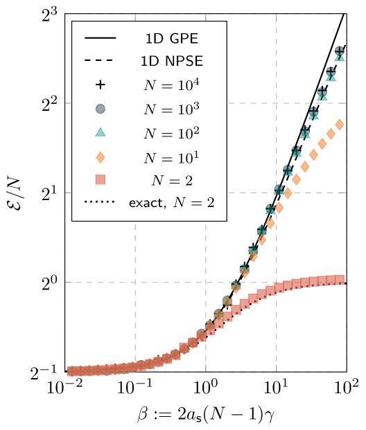
Figure 1: The ground-state energy per boson, as a function of the parameter $\beta$, for the 1D GPE and 1D NPSE, as defined in Eqs. (28), (29), and (30) along with the ground-state energy derived from the 2-RDM whilst enforcing the D and G conditions, for $N=2,10^{1},10^{2},10^{3}$, and $N=10^{4}$. In each case, $\gamma=10$, and the scattering length can be determined for each $N$ based on the value of $\beta$. The analytic Busch [12] is also provided by the dotted line.

Fig. 1 demonstrates the universality of the 2-RDM method in describing systems of particles from $N=2$ to $N=10^{4}$. Moreover, it allows us to identify the regime in which mean-field approaches become accurate. For example, the mean-field approach is poor at approximating the ground-state for a moderate, $N\sim 10$, number of bosons yet, in the case where $N\geq 100$, the mean-field regime, particularly when modelled by the 1D NPSE, become accurate.

We also demonstrate the capacity of the 2-RDM methodology to capture the complex attributes of systems with strong interactions. We consider a TG gas (where the harmonic trapping is included in the Hamiltonian), i.e., our system in the case that $g_{\mathsf{1D}},\beta\to\infty$. In such a case, the wavefunction is analytic, being equivalent to the non-interacting fermionic state of a single Slater determinant of the lowest $N$ particle states (this is the celebrated Fermi-Bose mapping theorem of Girardeau [6, 67]). As such we can extract the pair correlation function and the ground-state energy, the latter being the energy of a system of spinless fermions,

$$\mathcal{E}_{\mathsf{TG}}=\frac{N^{2}}{2}.$$ (31)

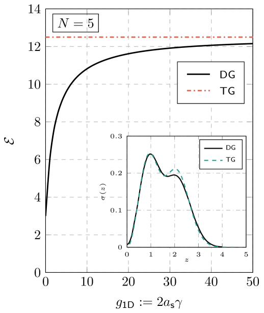
Figure 2: The ground-state energy $\mathcal{E}$ of the $N=5$ boson system, as a function of the parameter $g_{\mathsf{1D}}$, as derived from the 2-RDM method (solid line). We also plot the energy of the TG gas for the $N=5$ system as given in Eq. (31) (dashed line). The inset shows the diagonal pair correlation function $\sigma(z,0)$, as defined in Eq. (33), as a function of $z$ for the analytic TG wavefunction and that derived from the 2-RDM method (solid line) for $g_{\mathsf{1D}}=50$.

In Fig. 2 we plot the ground state energy, $\mathcal{E}$, of the $N=5$ system as a function of the interaction strength $g_{\mathsf{1D}}$, with the dash-dotted red line indicating the energy of the equivalent TG state, i.e., $\mathcal{E}=12.5$. Moreover, we demonstrate the extent to which the 2-RDM captures the ‘fermionisation’ of the boson system at large interaction strengths, which is manifest in the pair correlation function reducing to zero at the origin, $\sigma(z,0)\sim 0$ in the limit that $z\to 0$, where

$$\sigma(z,0) \coloneqq{}^{(2)}D(z,0;z,0)$$ (32)

$$=\sum_{ijkl}{}^{(2)}D^{ij}_{kl}\varphi_{i}(z)\varphi_{j}(0)\varphi_{k}(z)\varphi_{l}(0).$$ (33)

In the inset, $\sigma(z,0)$ is plotted as a function of $z$ for the 2-RDM method at $g_{\mathsf{1D}}=50$ and the TG gas. It is evident that the fermionisation is well-captured, as indicated by the suppression of $\sigma(z,0)$ at $z=0$ in the inset, and the convergence of the ground-state energy via the 2-RDM method to the TG limit. The limitations, in both cases, is a consequence of the choice of basis (which does not accurately capture the cusp in the wavefunction that is apparent due to the Dirac-$\delta$ interaction) and the finite basis rank.

III.2 Densities

The ground-state energy of our boson system is highly degenerate and we therefore also analyse structural aspects of the ground-state, such as the density, to test the 2-RDM methodology. The density is derivable from the 1-RDM as per,

$$\rho(z) \coloneqq{}^{(1)}D(z,z)$$ (34)

$$=\sum_{ij}{}^{(1)}D^{i}_{j}\varphi_{i}^{*}(z)\varphi_{j}(z).$$ (35)

In Fig. 3 we plot the ground-state density of the $N=10^{3}$ system for two different interaction strengths $\beta=10$ and $10^{3}$, where $\gamma=10$ in all cases. The density as derived from the RDM methodology is given by the dashed red line, the 1D GPE (solid black line), and 1D NPSE (dash-dotted black line).

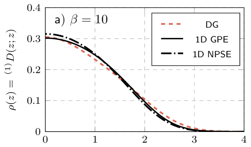
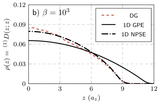
Figure 3: The ground-state density as a function of $z$ for two different values of $\beta$: $\beta=10$ in panel a) and $\beta=10^{3}$ in panel b). In all cases, $N=10^{3}$ and $\gamma=10$ and therefore the scattering length in each case can be duly determined. Furthermore, in all cases, we plot the density derived from the RDM methodology (dashed red line), the 1D GPE (solid black line), and 1D NPSE (dash-dotted black line).

The interaction strengths in Fig. 3 cover two separate regimes: relatively weakly interacting at $\beta=10$ and strongly interacting at $\beta=10^{3}$. In the former, the RDM density, the 1D GPE, and the 1D NPSE agree, indicating that the RDM method accurately reflects in the mean-field result for appropriate interaction strengths. However, for the latter case, where the interactions begin to dominate the ground-state, and the 1D GPE fails to capture the density, the RDM density agrees well with the density derived from the 1D NPSE. These results collectively demonstrate the capacity of the RDM methodology to capture structural properties of the ground-state for large particle numbers (i.e., $N=10^{3}$) and up to large interaction strengths $\beta=10^{3}$.

We note that, due to the use of a limited basis (of rank $20$) for the RDM methodology, very small ripples appear within the density, particular for panel b) in Fig. 3; it is expected that in the limit of a large basis rank these ripples would disappear. Notably, these are not structural ripples that reflect complex phenomenology within the ground-state, as, for example, indicated in the correlation function in the TG gas in Fig. 2. This is because $N=10^{3}$ is sufficiently larger to minimise these effects within the density profile.

III.3 Correlations

The correlation function was plotted in one instance for the $N=5$ system in Fig. 2 and here we analyse the correlation function in more detail. The correlation function provides us with details pertaining to the pair distribution of bosons, giving a numerical calculation of the likelihood of bosons being in proximity. In strongly interacting systems, such as the TG gas, the pair correlation function is naturally expected to be suppressed when the coordinates of bosons coincide.

In Fig. 4 we plot the pair correlation function $\sigma(z,0)$, which provides the likelihood of a boson being located at $z$ given another is located at the origin. This function is plotted for both $N=2$ and $N=10^{3}$ for a range of different interaction strengths $\beta=1,10,100$. In both cases, we identify a lack of suppression for small interaction strengths at the origin, and a large suppression as the interaction strengths increases. Moreover, this suppression is similar, both for the $N=2$ and $N=10^{3}$ cases; we note, however, that the suppression at $\beta=10$ for the $N=10^{3}$ case is less than than for the $N=2$ case, which is expected given the larger number of bosons.

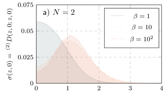
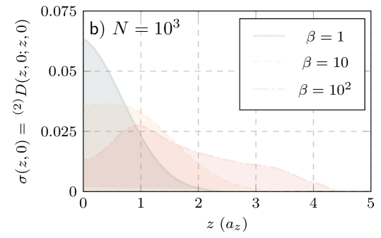
Figure 4: The ground-state correlation, $\sigma(z,0)$, as derived from the 2-RDM, as a function of $z$ for $N=2$ (panel a)) and $N=10^{3}$ (panel b)) and, in each case, for three different values of $\beta$: $\beta=1$ given by solid blue line, $\beta=10^{2}$ given by dashed orange line, and $\beta=10^{3}$ given by dash-dotted red line. In all cases, $\gamma=10$ and therefore the scattering length in each case can be duly determined.

The $N=2$ and $N=10^{3}$ cases constitute two extreme regimes, i.e., the few-body $(N=2)$ case with an analytic solution, and the $N=10^{3}$ case where mean-field descriptions are typically used. A key test of the RDM methodology is to study the crossover regime between these two cases, and identify if continuity is manifest in observable quantities. In Fig. 5 we plot the value of $\lim_{z\to 0}\sigma(z,0)\coloneqq\sigma(0,0)$ as a function of the interaction strength $\beta$ for a range of boson numbers $N=5,10,20,50,10^{2},$ and $10^{3}$. The plot demonstrates the continuous evolution of $\sigma(0,0)$ as $N$ increases, with no irregularities occurring within the crossover regime from few to many bosons. The consistency across $N$ and $\beta$ indicates that the RDM methodology successfully captures the key physical behaviours inherent to both few- and many-body systems.

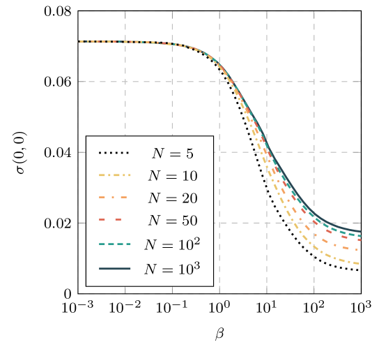
Figure 5: The value of the correlation function $\sigma(z,0)$ at the origin, i.e., $\sigma(0,0)=\lim_{z\to 0}\sigma(z,0)$ as a function of $\beta$ for $N=5$ to $N=10^{3}$ as indicated. In all cases, $\gamma=10$.

Of particular importance, the observed behaviour in the crossover regime (i.e., $N\sim 100$) indicates that the RDM methodology is robust in the regime where mean-field approaches are potentially inaccurate, but typical methods used for few-body systems are intractable. As such, it is arguable that the RDM methodology is universal, capable of capturing the properties of the ground-state across regimes that typically require a suite of different methods.

IV Concluding Remarks

In this work, we demonstrated the efficacy of the RDM methodology in describing bosonic systems comprising few to many particles. The RDM method has seen widespread success in the study of electronic structure in atomic and molecular systems yet had seen limited utilisation for bosons. Moreover, the RDM method had only been applied to systems consisting of short-range ‘contact’ interactions in our recent work [45]. As such, due to the lack of size-extensiveness of the 2-RDM, and the absence of the Pauli exclusion principle which places natural constraints on the size of basis used, the RDM method has been applied to large systems comprising $N=10^{3}$ to $10^{4}$ bosons across a range of (repulsive) interaction strength regimes.

Specifically, we demonstrate that the ground-state energy calculated via a variational procedure utilising the 2-RDM accurately reproduces the analytic results in the $N=2$ case, and aligns extremely well with highly accurate mean-field methods derived by Salasnich [10] for large particle numbers and strong interaction strengths. The RDM methodology therefore duly captures the ground-state energy across a range of extreme regimes, from small to large $N$ and $\beta$.

Additionally, the RDM methodology accurately reproduces the density as compared to the highly accurate mean-field descriptions for $N=10^{3}$; this accuracy is retained for large interaction strengths where the ‘standard’ 1D GPE fails dramatically. Moreover, the correlation function for $N=2$ and $N=10^{3}$ is given, with the expect heightening and suppression of the pair-correlation at the origin for small and large interaction strengths, respectively. These results collectively demonstrate the capacity of the RDM method to capture the structural properties of the ground state for few to many-boson systems.

A crucial test, however, is the capacity to accurately capture the ground-state in the crossover regime from few- to many-boson systems. We demonstrate the aptness of the RDM method by plotting the pair correlation function at the origin (i.e., the likelihood of finding two bosons at the origin) for a range of values of $N$, from $N=5$ to $N=10^{3}$. We identify a smooth transition of this quantity from the $N=5$ to the $N=10^{3}$ case, without any irregularities. As such, the crossover regime is well-captured.

The RDM method accordingly is well-suited to the description of bosonic systems regardless of the number of bosons. Notably, only the D and G conditions have been applied yet accurate results are obtained. As mentioned, this was also demonstrated by Gidofalvi et al [46] for a different one-dimensional bosonic system. Further tests of this method can be conducted, however, even on relatively simple systems. For example, the presence of solitons and droplets in 1D bosonic systems, as well as comparisons in the 3D case generally against the 3D GPE are distinct examples. Moreover, this method could be utilised to test the accuracy of the mean-field approaches for many-boson systems wherein there is disagreement with experiment. For example, corrections, nominally arising from quantum fluctuations, to the 3D GPE are typically made to account for the phenomenology of droplets in dipolar BECs [68]. The RDM method could therefore be utilised to more accurately describe this correction.

V Acknowledgements

M. J. K. is supported by an Australian Government Research Training Program Scholarship and by he University of Melbourne.

References

- Feshbach [1958] H. Feshbach, Ann. Phys. (N. Y.) 5, 357 (1958).
- Anderson et al. [1995] M. H. Anderson, J. R. Ensher, M. R. Matthews, C. E. Wieman, and E. A. Cornell, Science 269, 198 (1995).
- Görlitz et al. [2001] A. Görlitz, J. M. Vogels, A. E. Leanhardt, C. Raman, T. L. Gustavson, J. R. Abo-Shaeer, A. P. Chikkatur, S. Gupta, S. Inouye, T. Rosenband, and W. Ketterle, Phys. Rev. Lett. 87, 130402 (2001).
- Kinoshita et al. [2004] T. Kinoshita, T. Wenger, and D. S. Weiss, Science 305, 1125 (2004).
- Tonks [1936] L. Tonks, Phys. Rev. 50, 955 (1936).
- Girardeau [1960] M. Girardeau, Journal of Mathematical Physics 1, 516 (1960).
- Lieb and Liniger [1963] E. H. Lieb and W. Liniger, Phys. Rev. 130, 1605 (1963).
- Gross [1961] E. P. Gross, Il Nuovo Cimento 20, 454 (1961).
- Pitaevskii [1961] L. P. Pitaevskii, Sov. Phys. JETP 13, 451 (1961).
- Salasnich et al. [2002] L. Salasnich, A. Parola, and L. Reatto, Phys. Rev. A 65, 043614 (2002).
- Bao and Cai [2012] W. Bao and Y. Cai, arXiv preprint arXiv:1212.5341 (2012).
- Busch et al. [1998] T. Busch, B.-G. Englert, K. Rzażewski, and M. Wilkens, Found. Phys. 28, 549 (1998).
- Krauth [1996] W. Krauth, Phys. Rev. Lett. 77, 3695 (1996).
- Purwanto and Zhang [2004] W. Purwanto and S. Zhang, Phys. Rev. E 70, 056702 (2004).
- Vänskä et al. [2007] T. Vänskä, D. Sundholm, and M. Lindberg, Phys. Rev. A 75, 023621 (2007).
- Cederbaum et al. [2006] L. S. Cederbaum, O. E. Alon, and A. I. Streltsov, Phys. Rev. A 73, 043609 (2006).
- Bhowmik and Alon [2024] A. Bhowmik and O. E. Alon, J. Chem. Phys. 160, 044105 (2024), https://pubs.aip.org/aip/jcp/article-pdf/doi/10.1063/5.0176145/18702728/044105_1_5.0176145.pdf .
- Harteee [1928a] D. R. Harteee, Mathematical Proceedings of the Cambridge Philosophical Society 24, 89 (1928a).
- Harteee [1928b] D. R. Harteee, Mathematical Proceedings of the Cambridge Philosophical Society 24, 111 (1928b).
- Fock [1930a] V. A. Fock, Zeitschrift für Physik 61, 126 (1930a).
- Fock [1930b] V. A. Fock, Zeitschrift für Physik 62, 795 (1930b).
- Esry [1997] B. D. Esry, Phys. Rev. A 55, 1147 (1997).
- Bergeman [1997] T. Bergeman, Phys. Rev. A 55, 3658 (1997).
- Öhberg and Stenholm [1998] P. Öhberg and S. Stenholm, Phys. Rev. A 57, 1272 (1998).
- Benavides-Riveros et al. [2020] C. L. Benavides-Riveros, J. Wolff, M. A. L. Marques, and C. Schilling, Phys. Rev. Lett. 124, 180603 (2020).
- Mazziotti [2002] D. A. Mazziotti, Phys. Rev. A 65, 062511 (2002).
- Mazziotti [2012a] D. A. Mazziotti, Chem. Rev. 112, 244 (2012a).
- Zhao et al. [2004] Z. Zhao, B. J. Braams, M. Fukuda, M. L. Overton, and J. K. Percus, J. Chem. Phys. 120, 2095 (2004).
- Nakata et al. [2001] M. Nakata, H. Nakatsuji, M. Ehara, M. Fukuda, K. Nakata, and K. Fujisawa, J. Chem. Phys. 114, 8282 (2001).
- Fukuda et al. [2007] M. Fukuda, B. J. Braams, M. Nakata, M. L. Overton, J. K. Percus, M. Yamashita, and Z. Zhao, Math. Program. 109, 553 (2007).
- Nakata et al. [2008] M. Nakata, B. J. Braams, K. Fujisawa, M. Fukuda, J. K. Percus, M. Yamashita, and Z. Zhao, J. Chem. Phys. 128, 164113 (2008).
- Mazziotti [2012b] D. A. Mazziotti, Chem. Rev. 112, 244 (2012b).
- Mazziotti [2004a] D. A. Mazziotti, Phys. Rev. Lett. 93, 213001 (2004a).
- Mazziotti [2004b] D. A. Mazziotti, J. Chem. Phys. 121, 10957 (2004b).
- Mazziotti [2011] D. A. Mazziotti, Phys. Rev. Lett. 106, 083001 (2011).
- Rosina and Garrod [1975] M. Rosina and C. Garrod, J. Comput. Phys. 18, 300 (1975).
- DePrince and Mazziotti [2010] I. DePrince, A. Eugene and D. A. Mazziotti, J. Chem. Phys. 132, 034110 (2010), https://pubs.aip.org/aip/jcp/article-pdf/doi/10.1063/1.3283052/15667691/034110_1_online.pdf .
- Maradzike et al. [2020] E. Maradzike, M. Hapka, K. Pernal, and A. E. DePrince III, J. Chem. Theory Comput. 16, 4351 (2020).
- DePrince III and Mazziotti [2008] A. E. DePrince III and D. A. Mazziotti, J. Phys. Chem. B 112, 16158 (2008).
- Mazziotti [2020] D. A. Mazziotti, Phys. Rev. A 102, 052819 (2020).
- Head-Marsden and Mazziotti [2020] K. Head-Marsden and D. A. Mazziotti, J. Phys. Chem. A 124, 4848 (2020).
- Anderson et al. [2013] J. S. Anderson, M. Nakata, R. Igarashi, K. Fujisawa, and M. Yamashita, Computational and Theoretical Chemistry 1003, 22 (2013).
- Hammond and Mazziotti [2006] J. R. Hammond and D. A. Mazziotti, Phys. Rev. A 73, 062505 (2006).
- Verstichel et al. [2012] B. Verstichel, H. van Aggelen, W. Poelmans, and D. Van Neck, Phys. Rev. Lett. 108, 213001 (2012).
- Knight et al. [2022] M. J. Knight, H. M. Quiney, and A. M. Martin, New J. Phys. 24, 053004 (2022).
- Gidofalvi and Mazziotti [2004] G. Gidofalvi and D. A. Mazziotti, Phys. Rev. A 69, 042511 (2004).
- Coleman [1963] A. J. Coleman, Rev. Mod. Phys. 35, 668 (1963).
- Garrod and Percus [1961] C. Garrod and J. K. Percus, J. Math. Phys. 5, 659 (1961).
- Mazziotti [2012c] D. A. Mazziotti, Phys. Rev. A 85, 062507 (2012c).
- Mazziotti [2012d] D. A. Mazziotti, Phys. Rev. Lett. 108, 263002 (2012d).
- Mazziotti [2006] D. A. Mazziotti, Phys. Rev. A 74, 032501 (2006).
- Husimi [1940] K. Husimi, Proc. Phys.-Math. Soc. Jap. Ser. 3. 22, 264 (1940).
- Löwdin [1955] P.-O. Löwdin, Phys. Rev. 97, 1474 (1955).
- ter Haar [1961] D. ter Haar, Rep. Prog. Phys. 24, 304 (1961).
- McWeeny [1960] R. McWeeny, Rev. Mod. Phys. 32, 335 (1960).
- Mayer [1955] J. E. Mayer, Phys. Rev. 100, 1579 (1955).
- Tredgold [1957] R. H. Tredgold, Phys. Rev. 105, 1421 (1957).
- Vandenberghe and Boyd [1996] L. Vandenberghe and S. Boyd, SIAM Rev. 38, 49 (1996).
- Gärtner and Matousek [2012] B. Gärtner and J. Matousek, Approximation Algorithms and Semidefinite Programming (Springer-Verlag, 2012).
- Yamashita et al. [2010] M. Yamashita, K. Fujisawa, K. Nakata, M. Nakata, M. Fukuda, K. Kobayashi, and K. Goto, A high-performance software package for semidefinite programs: SDPA 7, Tech. Rep. (Research Report B-460, Department of Mathematical and Computing Science, Tokyo Institute of Technology, Tokyo, 2010).
- Yamashita et al. [2012] M. Yamashita, K. Fujisawa, M. Fukuda, K. Kobayashi, K. Nakata, and M. Nakata, Latest developments in the SDPA family for solving large-scale SDPs, in Handbook on Semidefinite, Conic and Polynomial Optimization, edited by M. F. Anjos and J. B. Lasserre (Springer US, Boston, MA, 2012) pp. 687–713.
- Zhao et al. [2010] X.-Y. Zhao, D. Sun, and K.-C. Toh, SIAM Journal on Optim. 20, 1737 (2010).
- Yang et al. [2015] L. Yang, D. Sun, and K.-C. Toh, Math. Program. Optim. 7, 331 (2015).
- Sun et al. [2020] D. Sun, K.-C. Toh, Y. Yuan, and X.-Y. Zhao, Optim. Methods Softw. 35, 87 (2020).
- Sun et al. [2008] D. Sun, J. Sun, and L. Zhang, Math. Program. 114, 349 (2008).
- Meade et al. [2017] B. Meade, L. Lafayette, G. Sauter, and D. Tosello, Spartan hpc-cloud hybrid: Delivering performance and flexibility (2017).
- Yukalov and Girardeau [2005] V. I. Yukalov and M. D. Girardeau, Laser Physics Letters 2, 375 (2005).
- Ferrier-Barbut et al. [2016] I. Ferrier-Barbut, H. Kadau, M. Schmitt, M. Wenzel, and T. Pfau, Phys. Rev. Lett. 116, 215301 (2016).