Recognizing and Realizing Temporal Reachability Graphs

Abstract

A temporal graph $\mathcal{G}=(G,\lambda)$ can be represented by an underlying graph $G=(V,E)$ together with a function $\lambda$ that assigns to each edge $e\in E$ the set of time steps during which $e$ is present. The reachability graph of $\mathcal{G}$ is the directed graph $D=(V,A)$ with $(u,v)\in A$ if only if there is a temporal path from $u$ to $v$. We study the Reachability Graph Realizability (RGR) problem that asks whether a given directed graph $D=(V,A)$ is the reachability graph of some temporal graph. The question can be asked for undirected or directed temporal graphs, for reachability defined via strict or non-strict temporal paths, and with or without restrictions on $\lambda$ (proper, simple, or happy). Answering an open question posed by Casteigts et al. (Theoretical Computer Science 991 (2024)), we show that all variants of the problem are NP-complete, except for two variants that become trivial in the directed case. For undirected temporal graphs, we consider the complexity of the problem with respect to the solid graph, that is, the graph containing all edges that could potentially receive a label in any realization. We show that the RGR problem is polynomial-time solvable if the solid graph is a tree and fixed-parameter tractable with respect to the feedback edge set number of the solid graph. As we show, the latter parameter can presumably not be replaced by smaller parameters like feedback vertex set or treedepth, since the problem is W[2]-hard with respect to these parameters.

1 Introduction

Temporal graphs are graphs whose edge set can change over time. The vertex set is often assumed to be fixed, and the edge set can differ from one time step to the next. The study of temporal graphs has attracted significant attention in recent years [4, 20, 21]. A temporal graph $\mathcal{G}$ with vertex set $V$ can be represented as a sequence $(G_{i})_{i\in[L]}$, where $G_{i}=(V,E_{i})$ is the graph containing the edges that are present in time step $i$. An alternative way to represent $\mathcal{G}$ is to specify a graph $G=(V,E)$ together with a labeling function $\lambda:E\to 2^{[L]}$ that maps each edge $e\in E$ to the (possibly empty) set of time steps in which $e$ is present. We write $\mathcal{G}=(G,\lambda)$ in this case. If an edge $e$ is present in time step $i$, we refer to $(e,i)$ as a time edge. A strict temporal path from $u$ to $v$ in $\mathcal{G}$ is a sequence of time edges such that the edges form a $u$-$v$-path in the underlying graph and the time steps are strictly increasing. A non-strict temporal path is defined analogously, except that the time steps only need to be non-decreasing. Given a temporal graph $\mathcal{G}$, the reachability relation (with respect to strict or non-strict temporal paths) can be represented as a directed graph $D=(V,A)$, called the reachability graph, with $(u,v)\in A$ for $u\neq v$ if and only if there exists a (strict or non-strict, respectively) temporal path from $u$ to $v$ in $\mathcal{G}$. Note that self-loops, which would represent the trivial reachability from a vertex to itself, are omitted from $D$.

A natural question is then which directed graphs $D=(V,A)$ can arise as reachability graphs of temporal graphs, and how difficult it is to determine for a given directed graph $D=(V,A)$ whether there exists a temporal graph $\mathcal{G}$ with reachability graph $D$. This question was posed as an open problem by Casteigts et al. [3, Open question 5]. In this paper, we answer this open question by showing that this decision problem is NP-hard. Actually, there are a number of variations of the question, as we may ask for an undirected or a directed temporal graph $\mathcal{G}$, for a temporal graph with a restricted kind of labeling (simple, proper, happy), and may consider reachability with respect to strict or non-strict temporal paths. We show that all these variations are NP-hard if we ask for an undirected temporal graph, and also if we ask for a directed temporal graph except for two variations (strict temporal paths with arbitrary or simple labelings) that are known to become trivial in the directed case [10]. See Table 1 for an overview of these complexity results.

From the positive side, we present the following algorithmic results. For a given digraph $D=(V,A)$, we refer to $\{u,v\}$ for $u,v\in V$ as a solid edge if both $(u,v)$ and $(v,u)$ are in $A$. Let $G=(V,E)$ be the undirected graph on $V$ whose edge set is the set of solid edges. We refer to $G$ as the solid graph of $D$. We show that all undirected problem variants can be solved in polynomial time if the solid graph is a tree. Furthermore, we give an FPT algorithm with respect to the feedback edge set number of the solid graph. This parameter can presumably not be replaced by smaller parameters like feedback vertex set, treedepth, or pathwidth, since two undirected versions of our problem turn out to be W[2]-hard for these parameters.

Table 1: The complexity results for all variants of RGR. Red cells indicate NP-hard cases and green cells indicate cases that are trivial (and thus polynomial-time solvable).

	Strict	Non-strict
Any	Theorem˜6.1	Theorem˜6.3
Simple	Theorem˜6.1	Theorem˜6.3
Proper	Theorem˜6.3
Happy	Theorem˜6.3

(a) undirected

	Strict	Non-strict
Any	Lemma˜8.1 and [10]	Theorem˜8.7
Simple	Lemma˜8.1 and [10]	Theorem˜8.7
Proper	Theorem˜8.7
Happy	Theorem˜8.7

(b) directed

Related work

Casteigts et al. [3] studied the relationships between the classes of reachability graphs that arise from undirected temporal graphs if different restrictions are placed on the graph (proper, simple, happy [3]) and depending on whether strict or non-strict temporal paths are considered. They showed that reachability with respect to strict temporal paths in arbitrary temporal graphs yields the widest class of reachability graphs while reachability in happy temporal graphs yields the narrowest class. The class of reachability graphs that arise from proper temporal graphs is the same as for non-strict paths in arbitrary temporal graphs, and this class is larger than the class of reachability graphs arising from non-strict reachability in simple temporal graphs. Strict reachability in simple temporal graphs was also shown to lie between the happy case and the general strict case. Döring [10] showed that the class “strict & simple” is incomparable to “non-strict & simple” and to “non-strict / proper”, completing the picture of a two-stranded hierarchy for undirected temporal graphs. She also extended the study to directed temporal graphs and showed that their classes of reachability graphs form a single-stranded hierarchy from happy to strict & simple, the latter being equivalent to the general strict case.

Casteigts et al. [3] posed the open question whether there is a characterization of the directed graphs that arise as reachability graphs of temporal graphs (or of some restricted subclass of temporal graphs), and how hard it is to decide whether a given directed graph is the reachability graph of some temporal graph. These questions were posed again by Döring [10], also in relation to the setting of directed temporal graphs. This is in particular of interest because Casteigts et al. [5] showed that several temporal graph problems can be solved in FPT time with respect to temporal parameters defined over the reachability graph. In this paper we resolve these open questions regarding the complexity of all directed and undirected variants.

Besides that, our work falls into the field of temporal graph realization problems. In these problems, one is given some data about the behavior of a temporal graph, and the goal is to detect whether there actually is a temporal graph with this behavior (and to compute such a temporal graph if one exists). Klobas et al. [16] introduced the problem of deciding for a given matrix of fastest travel durations and a period $\Delta$ whether there exists a simple temporal graph $\mathcal{G}$ with period $\Delta$ with the property that the duration of the fastest temporal path between any pair of nodes in $\mathcal{G}$ is equal to the value specified in the input matrix. Erlebach et al. [12] extended the problem to a multi-label version, assuming that the input specifies a bound $\ell$ on the maximum number of labels per edge.

Motivated by the constraints in the design of transportation networks, Mertzios et al. [19] considered the modified version of the problem (with one label per edge) where the fastest temporal path between any pair of nodes is only upper-bounded by the value specified in the input matrix.

The problem of generating a temporal graph realizing a given reachability graph is an instance of the more general class of temporal network design problem. In such problems, the objective is to construct a temporal network that satisfies specified constraints while optimizing certain network-quality measures. These problems have natural applications in transportation and logistics, communication networks, social networks, and epidemiology. In an early example studied by Kempe et al. [14], the goal was to reconstruct a temporal labeling restricted to a single label per edge, so that a designated root reaches via temporal paths all vertices in a set $P$ while avoiding those in a set $N$. For multi-labeled temporal graphs, Mertzios et al. [18] studied the problem of designing a temporal graph that preserves all reachabilities or paths of an underlying static graph while minimizing either the temporality (the maximum number of labels per edge) or the temporal cost (the total number of labels used). Göbel et al. [13] showed that it is NP-complete to decide whether the edges of a given undirected graph can be labeled with a single label per edge in such a way that each vertex can reach every other vertex via a strict temporal path. Other studies have focused on variants of minimizing edge deletions [11], vertex deletions [24], or edge delays [8] to restrict reachability, motivated, for instance, by epidemic containment strategies that limit interactions. Temporal network design is an active area of research, with further related questions explored for example in [1, 15, 6]. For general introductory texts to the area of dynamic networks the reader is referred to [4, 20, 21].

Organization of the paper.

In Section˜2 we provide a formal problem definition and define the notions used in this work. In Section˜3, we show upper and lower bounds for the required number of labels per edge in any realization and provide a single exponential algorithm for all problem variants. Afterwards, in Section˜4, we analyze properties and define splitting operations based on bridge edges in the solid graph of the undirected versions of our problem. These structural insights will be mainly used in our FPT algorithm in Section˜7, but also immediately let us describe a polynomial-time algorithm for instances where the solid graph is a tree in Section˜5. In Section˜6, we then provide NP-hardness results for all undirected problem versions as well as parameterized intractability results for two of them with respect to feedback vertex set number and treedepth. Afterwards, in Section˜7, we provide our main algorithmic result: an FPT algorithm with respect to the feedback edge set number $\mathrm{fes}$ of the solid graph. This algorithm is achieved in three steps: Firstly, we apply our splitting operations of Section˜4 and provide a polynomial-time reduction rule to simplify the instance at hand, such that all we need to deal with is a subset $X^{*}$ of vertices of size $\mathcal{O}(\mathrm{fes})$ for which the remainder of the graph decomposes into edge-disjoint trees that only interact with $X^{*}$ via two leaves each. We call such trees connector trees. Secondly, we show that we can efficiently extend the set $X^{*}$ to a set $W^{*}$ of size $\mathcal{O}(\mathrm{fes})$ such that each respective connector tree is more or less independent from the remainder of the graph with respect to the interactions of temporal paths in any realization. All these preprocessing steps run in polynomial time. Afterwards, our algorithm enumerates all reasonable labelings on the edges incident with vertices of $W^{*}$ and tries to extend each such labeling to a realization for $D$. As we show, there are only FPT many such reasonable labelings and for each such labeling, there are only FPT many possible extensions that need to be checked. Finally, in Section˜8 we briefly discuss the directed version of the problem and provide NP-hardness results for all but the two trivial cases.

2 Preliminaries

For definitions on parameterized complexity, the Exponential Time Hypothesis (ETH), or parameters like treedepth, we refer to the textbooks [9, 7].

For natural numbers $i,j$ with $i\leq j$ we write $[i]$ for the set $\{1,2,3,\ldots,i\}$ and $[i,j]$ for the set $\{i,i+1,i+2,\ldots,j\}$. For an undirected graph $G=(V,E)$, we denote an edge between vertices $u$ and $v$ as $\{u,v\}$ or $uv$. By $N(v)=\{u\in V\mid vu\in E\}$ we denote the set of neighbors of $u$. The degree of $v$ is the size of $N(v)$. An edge $e\in E$ is a bridge or bridge edge in a graph $G=(V,E)$ if deleting $e$ increases the number of connected components. A vertex of degree $1$ is called a pendant vertex, and an edge incident with a pendant vertex is called a pendant edge.

For directed graphs, we denote an arc from $u$ to $v$ by $(u,v)$. A directed graph $D$ is simple if it has no parallel arcs and no self-loops, and it is a directed acyclic graph (DAG) if it does not contain a directed cycle. The in-degree of a vertex $v$ in $D$ is the number of incoming arcs of $v$, i.e., the number of arcs with head $v$. Similarly, the out-degree of a vertex $v$ is the number of arcs with tail $v$. The degree of a vertex in $D$ is then the sum of its in-degree and out-degree.

A temporal graph $\mathcal{G}$ with vertex set $V$ and lifetime $L$ is given by a sequence $(G_{t})_{t\in[L]}$ of $L$ static graphs $G_{t}=(V,E_{t})$ referred to as snapshots or layers. The graph $\mathcal{G}_{\downarrow}=(V,E_{\downarrow})$ with $E_{\downarrow}=\bigcup_{i\in[L]}E_{i}$ is called the underlying graph of $\mathcal{G}$. Alternatively, $\mathcal{G}$ can be represented by an undirected graph $G=(V,E)$ with $E\supseteq\bigcup_{t\in[L]}E_{t}$ and a labeling function $\lambda:E\to 2^{[1,L]}$ that assigns to each edge $e$ the (possibly empty) set of time steps during which $e$ is present, i.e., $\lambda(e)=\{t\in[L]\mid e\in E_{t}\}$. We write $\mathcal{G}=(G,\lambda)$ in this case. In this representation we allow $G$ to contain extra edges in addition to the edges of the underlying graph; such edges $e$ satisfy $\lambda(e)=\emptyset$. This is useful because in the problems we consider in this paper, there is a natural choice of a graph $G=(V,E)$, the so-called solid graph defined below, that contains all edges of the underlying graph of every realization but may contain additional edges.

We assume that each layer of a temporal graph is an undirected graph unless we explicitly refer to directed temporal graphs. If $t\in\lambda(e)$, we refer to $(e,t)$ as a time edge. A temporal path from $u$ to $v$ in $\mathcal{G}$ is a sequence of time edges $((e_{j},t_{j}))_{j\in[\ell]}$ for some $\ell$ such that $(e_{1},e_{2},\ldots,e_{\ell})$ is a $u$-$v$ path in $G$ and $t_{1}\leq t_{2}\leq\cdots\leq t_{\ell}$ holds in the non-strict case and $t_{1}<t_{2}<\cdots<t_{\ell}$ holds in the strict case.

A temporal graph is proper if no two adjacent edges share a label, simple if every edge has a single label, and happy if it is both proper and simple [3]. Note that for proper and happy temporal graphs there is no distinction between strict and non-strict temporal paths.

The reachability graph $\mathcal{R}(\mathcal{G})$ of a temporal graph $\mathcal{G}$ with vertex set $V$ is the directed graph $(V,A)$ with the same vertex set $V$ and $(u,v)\in A$ if and only if $u\neq v$ and $\mathcal{G}$ contains a temporal path from $u$ to $v$. Note that $\mathcal{R}(\mathcal{G})$ depends on whether we consider strict or non-strict temporal paths and can be computed in polynomial time in both cases [2].

We are interested in the following problem:

Reachability Graph Realizability (RGR)
Input: A simple directed graph $D=(V,A)$.
Question: Does there exist a temporal graph $\mathcal{G}$ with $\mathcal{R}(\mathcal{G})=D$?

For yes-instances of RGR, we are also interested in computing a temporal graph $\mathcal{G}$ with $\mathcal{R}(\mathcal{G})=D$. We refer to such a temporal graph as a solution or a realization for $D$, and we typically represent it by a labeling function. With the adjacency matrix representation of $D$ in mind, we also write $D_{uv}=1$ for $(u,v)\in A$ and $D_{uv}=0$ for $(u,v)\notin A$.

We can consider RGR with respect to reachability via strict temporal paths or with respect to non-strict temporal paths. Furthermore, we can require the realization of $D$ to be simple, proper, or happy. For proper and happy temporal graphs, strict and non-strict reachability coincide. Therefore, the distinct problem variants that we can consider are Any Strict RGR, Any Non-strict RGR, Simple Strict RGR, Simple Non-strict RGR, Proper RGR, and Happy RGR. Finally, we write DRGR instead of RGR if we are asking for a directed temporal graph that realizes $D$. We sometimes write URGR if we want to make it explicit that we are asking for an undirected realization.

The solid graph.

If $D_{uv}=1$ and $D_{vu}=1$ for some $u\neq v$, we say that there is a solid edge between $u$ and $v$. If $D_{uv}=1$ and $D_{vu}=0$, we say that there is a dashed arc from $u$ to $v$. We use $G=(V,E)$ to denote the graph on $V$ whose edge set is the set of solid edges, and we refer to this graph as the solid graph (of $D$). It is clear that only solid edges can receive labels in a realization of $D$, as the two endpoints of an edge that is present in at least one time step can reach each other. Solid edges that are bridges of the solid graph must receive labels, but a solid edge $e$ that is not a bridge need not necessarily receive labels, as the endpoints of $e$ could reach each other via temporal paths of length greater than one in a realization. Let $D$ be an instance of URGR. Let $\lambda$ be a realization of $D$ and let $\{u,v\}$ and $\{v,w\}$ be solid edges that both receive at least one label under $\lambda$. If $D$ contains neither the arc $(u,w)$ nor the arc $(w,u)$, then there is a label $\alpha$ such that $\lambda(\{u,v\})=\lambda(\{v,w\})=\{\alpha\}$. Note that Observation 2 implies that for Proper URGR, Happy URGR, and Non-strict URGR, no realization for $D$ can assign labels to both of two adjacent edges $\{u,v\}$ and $\{v,w\}$ if $D$ contains neither $(u,w)$ nor $(w,u)$.

A path $P=(u_{0}=u,u_{1},u_{2},\ldots,u_{\ell}=v)$ from $u$ to $v$ in $G$ is a dense $u$-$v$-path if there exist dashed arcs $(u_{i},u_{j})$ for all $0\leq i<j\leq\ell$. Note that in each undirected realization of $D$, each temporal path is a dense path in $G$. Similarly, for directed realizations of $D$, each temporal path is a dense path in $D$, where we define dense paths in $D$ analogously to dense paths in $G$.

We say that a realization $\lambda$ is frugal if there is no edge $e$ such that the set of labels assigned to $e$ can be replaced by a smaller set while maintaining the property that $\lambda$ is a realization. We say that a realization $\lambda$ is minimal on edge $e$ if it is impossible to obtain another realization by replacing $\lambda(e)$ with a proper subset. A realization is minimal if it is minimal on every edge $e$. Note that every frugal realization is also minimal.

3 Basic Observations and an Exponential Algorithm

We first provide upper and lower bounds for the number of labels per edge in a minimal realization.

Lemma 3.1.

Let $D$ be an instance of URGR, and let $e$ be a solid edge of $G$ that is not part of a triangle. In each minimal realization of $D$, $e$ receives at most two labels. Moreover, if $D$ is an instance of any version of URGR besides Any Strict URGR, then in each minimal realization, $e$ receives at most one label.

Proof 3.2.

First, consider Any Strict URGR. Consider a minimal realization and assume the edge $e$ has at least three labels. Let $L_{e}$, $U_{e}$, and $M_{e}$ be its smallest label, its largest label, and an arbitrary label in between. Note that no solid edge $f\neq e$ incident with an endpoint of $e$ can have a label in $(L_{e},U_{e})$ as this would imply a solid edge forming a triangle containing $e$. Hence, all other edges incident with endpoints of $e$ only have labels $\leq L_{e}$ or $\geq U_{e}$. Replacing the labels of $e$ by the single label $M_{e}$ maintains exactly the temporal paths containing $e$ that exist before the change, a contradiction to the original realization being minimal. Furthermore, if the original labeling was proper, than the resulting labeling is also proper.

For Simple Strict URGR, Simple Non-strict URGR and Happy URGR, it is trivially true that $e$ has at most one label in any realization. Now, consider Any Non-strict URGR and Proper URGR. Assume that $e$ has at least two labels in a minimal realization, and let $L_{e}$ and $U_{e}$ be the smallest and largest label of $e$. Note that no solid edge $f\neq e$ incident with an endpoint of $e$ can have a label in $[L_{e},U_{e}]$: A label in $(L_{e},U_{e})$ would create a solid edge forming a triangle, $f$ cannot share a label with $e$ in a proper labeling, and $f$ sharing a label with $e$ would create a solid edge forming a triangle in the non-strict case. Thus, all other edges incident with endpoints of $e$ only have labels $<L_{e}$ or $>U_{e}$. Replacing the labels of $e$ by $L_{e}$ maintains exactly the temporal paths containing $e$ that exist before the change, a contradiction to the original realization being minimal.

For general edges, we show a linear upper bound with respect to the number of vertices.

Lemma 3.3.

If a graph $D=(V,A)$ is realizable, then each minimal realization for $D$ assigns at most $n=|V|$ labels per edge.

Proof 3.4.

Let $e$ be an edge with more than $n$ labels. We show that at least one can be removed. For each vertex $v$ define $\alpha_{v}$ as the earliest time step in which vertex $v$ can traverse the edge $e$ (if any). Let $\beta$ be a label of $e$ that is unequal to all $\alpha_{v}$ labels. Then, removing $\beta$ from $e$ preserves at least one temporal $(x,y)$-path, if such a path existed before.

Note that this implies that all versions of URGR and DRGR under consideration are in NP. Next, we show that this bound on the number of labels per edge is essentially tight for Any Strict URGR.

Theorem 3.5.

For Any Strict URGR, there is an infinite family of directed graphs $\mathcal{B}$, such that for every $D=(V,A)\in\mathcal{B}$, where $G=(V,E)$ is the solid graph of $D$, all of the following properties hold:

• $G$ is planar.

• $G$ has a feedback vertex set of size 2 and a feedback edge set of size $\Theta(n)$, where $n=|V|$.

• $D$ is realizable and there is an edge $e\in E$ such that every realization of $D$ uses $\Omega(n)$ labels on $e$.

Proof 3.6.

The graphs of solid edges of the reachability graphs in $\mathcal{B}$ resemble books with vertices around the sides of their pages. The spine of the book consists of an edge $u_{0}u^{\prime}_{0}$ joining an upper spine-vertex $u_{0}$ and a lower spine-vertex $u^{\prime}_{0}$. Every page has an index $1\leq i\leq L$, where $L\geq 5$ is the total number of pages, and consists of two upper vertices, $u_{i}$ and $v_{i}$, and two lower vertices, $u^{\prime}_{i}$ and $v^{\prime}_{i}$, located at the middle and end of the upper and lower boundaries, respectively. We call $u_{i}$ and $u^{\prime}_{i}$ the inner and $v_{i}$ and $v^{\prime}_{i}$ the outer vertices of page $i$. The set of edges of page $i$ consists of edges $u_{0}u_{i}$, $u_{i}v_{i}$, $v_{i}v^{\prime}_{i}$, $u^{\prime}_{i}v^{\prime}_{i}$, and $u^{\prime}_{0}u^{\prime}_{i}$, around the sides of the page, as well as two additional diagonal edges, $u_{0}u^{\prime}_{i}$ and $u^{\prime}_{0}u_{i}$, between the spine and the inner vertices. We then modify the constructed graph by making pages $1$, $2$, $L-1$ and $L$ incomplete: For $i=1,2$, page $i$ does not contain the lower-side vertices $u_{i}^{\prime}$ and $v_{i}^{\prime}$, and the diagonal between $u_{i}$ and $u_{0}^{\prime}$ is a dashed arc $(u_{i},u_{0}^{\prime})$ instead of a solid edge. For $i=L-1,L$, page $i$ does not contain the upper-side vertices $u_{i}$ and $v_{i}$, and the diagonal between $u_{i}^{\prime}$ and $u_{0}$ is a dashed arc $(u_{0},u_{i}^{\prime})$ instead of a solid edge. Furthermore, there is a dashed arc from every inner vertex of a page $i$ to every same-side (i.e., upper to upper and lower to lower) inner vertex of a page $j$ if and only if $i<j$ and both vertices exist, and there is a dashed arc to every opposite-side (i.e., upper to lower and lower to upper) inner vertex of a page $k$ if and only if $i+1<k$ and the target vertex exists. All remaining ordered pairs of vertices $(u,v)$ are specified as unreachable by $D$ (i.e., $(u,v)$ is not a dashed arc). See Figure 1(a). Note that $n=4(L-4)+2\cdot 4+2=4L-6$ and the solid graph has $m=7(L-4)+2\cdot 4+1=7L-19$ edges.

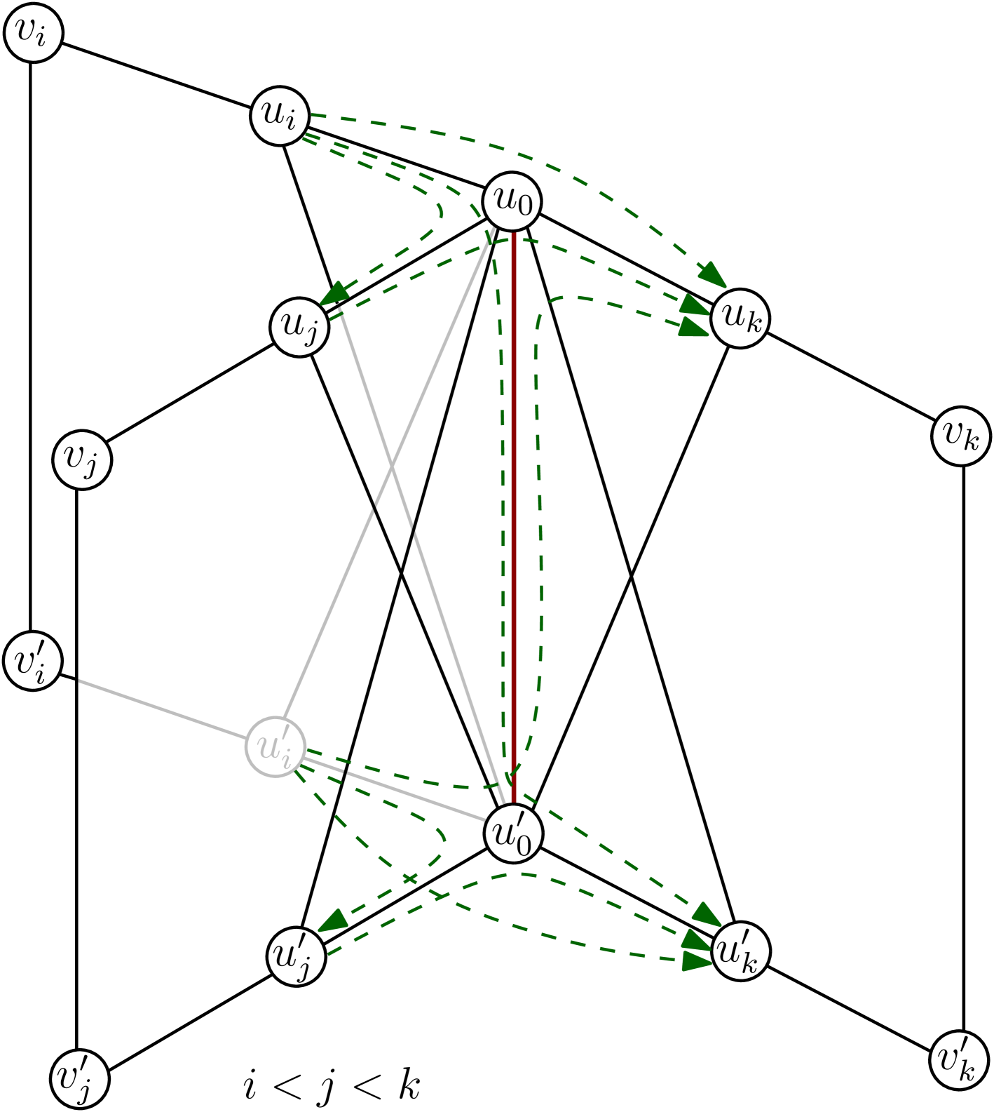
(a)

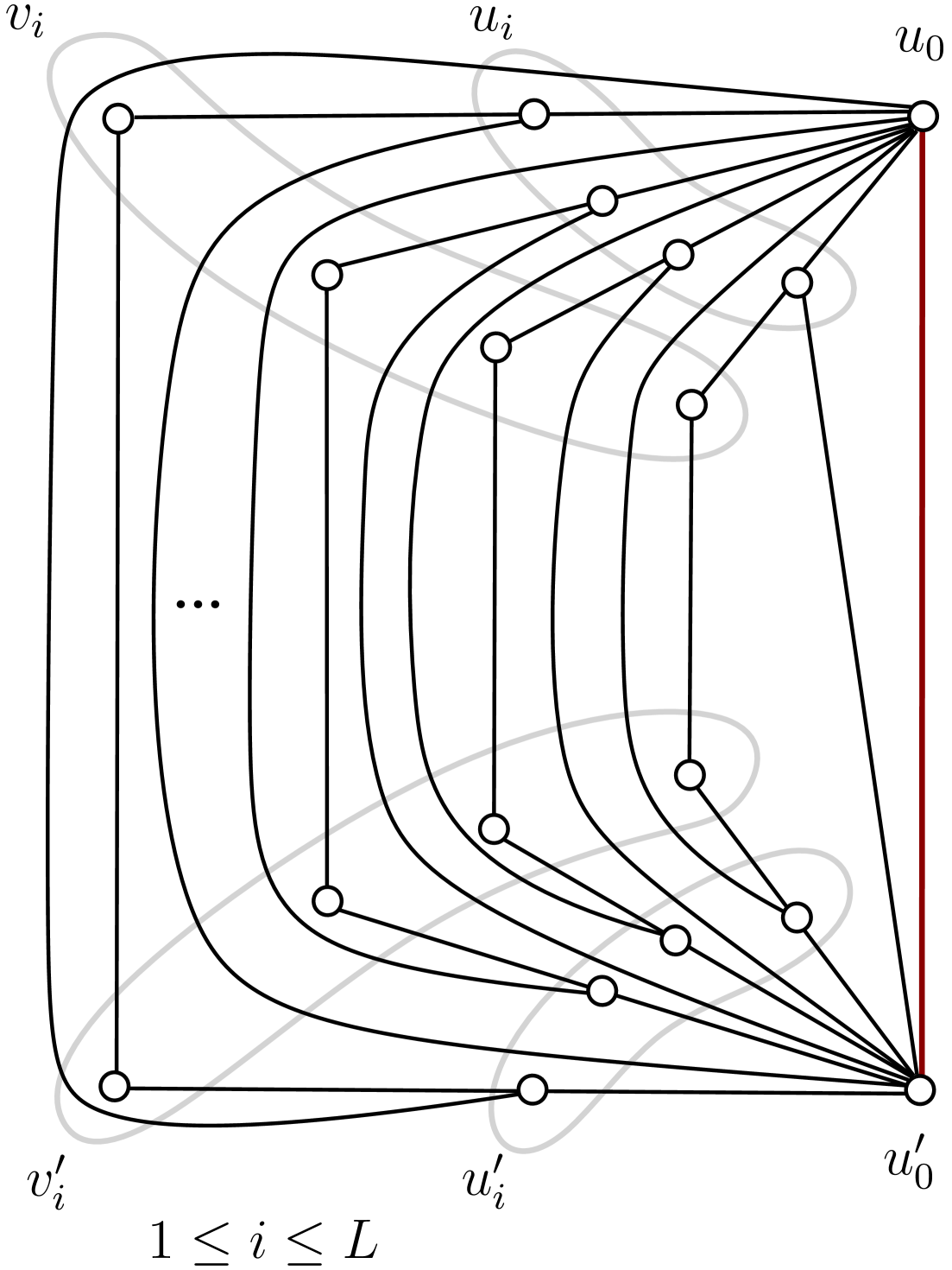
(b)

Figure 1: (a) An example of the graph of solid edges and dashed arcs for a $D\in\mathcal{B}$ restricted to three pages. (b) A planar drawing of the solid edges.

We start by proving the last property, fixing the edge $u_{0}u^{\prime}_{0}$ of the spine as the edge required by it. We will show that $u_{0}u^{\prime}_{0}$ must have at least $L-2=n/4-1/2=\Theta(n)$ labels. We claim that no two edges of a page $i$ can have distinct labels, so edges of page $i$ can be labeled by at most one label, which we denote by $l_{i}$. The two upper edges cannot have distinct labels, otherwise a missing arc between $u_{0}$ and $v_{i}$ would be realized. The same holds for the two lower edges. Similarly, $v_{i}v^{\prime}_{i}$ and the diagonal edges cannot have a label different from that of the upper and lower edges, otherwise a missing arc would be realized. This implies that the only way to realize the arcs of $v_{i}v^{\prime}_{i}$ is to label it by $l_{i}$. Edges $u_{i}v_{i}$ and $u^{\prime}_{i}v^{\prime}_{i}$ must also be labeled by $l_{i}$ as any other path to realize their arcs would need to use two consecutive edges of page $i$. For $i=1,2$, both upper edges of page $i$ must be labeled as they are bridges. For $i=L-1,L$, both lower edges of page $i$ must be labeled for the same reason. For $3\leq i\leq L-2$, at least one of the edges $u_{i}u_{0}$ and $u_{i}u_{0}^{\prime}$ must be labeled, and at least one of the edges $u_{i}^{\prime}u_{0}^{\prime}$ and $u_{i}^{\prime}u_{0}$ must be labeled, as the arcs between $u_{i}$ or $u_{i}^{\prime}$ and $u_{0}$ and $u_{0}^{\prime}$ cannot be realized otherwise. We will show that $u_{0}u_{i}$ and $u_{0}^{\prime}u_{i}^{\prime}$ receive a label (which must be equal to $l_{i}$) while the diagonals $u_{0}u_{i}^{\prime}$ and $u_{0}^{\prime}u_{i}$ do not receive a label. First, observe that $l_{j}>l_{i}$ must hold for any $j>i$, otherwise the arc $(u_{i},u_{j})$ or $(u_{i}^{\prime},u_{j}^{\prime})$ cannot be realized. Now, assume for a contradiction that there is a page $i$ with $3\leq i\leq L-2$ in which a diagonal receives a label. Consider the smallest such $i$. Observe that $u_{0}u_{i}^{\prime}$ cannot receive label $l_{i}$ as this would realize an arc $(u_{i-1},u_{i}^{\prime})$. Thus, $u_{i}^{\prime}u_{0}^{\prime}$ must receive label $l_{i}$. Furthermore, $u_{i}u_{0}$ must also receive label $l_{i}$ as the arc $(u_{i-1},u_{i})$ must be realized via the path $u_{i-1},u_{0},u_{i}$; it cannot be realized via a temporal path ending with the edge $u_{0}^{\prime}u_{i}$ as the existence of such a path would imply a temporal path from $u_{i-1}$ to $u_{i}^{\prime}$, a contradiction. Finally, edge $u_{i}u_{0}^{\prime}$ cannot receive a label; otherwise, $u_{i}$ can reach both $u_{0}$ and $u_{0}^{\prime}$ at time $l_{i}$ and therefore reach $u_{i+1}^{\prime}$ at time $l_{i+1}$, a contradiction. This shows that it is impossible that a diagonal edge in page $i$ receives a label. For every two distinct pages $i$ and $j$ such that $i<j$, the arcs from the inner vertices of $i$ to the same-side inner vertices of $j$ imply that $u_{0}u_{i}$, $u^{\prime}_{0}u^{\prime}_{i}$ and $u_{0}u_{j}$, $u^{\prime}_{0}u^{\prime}_{j}$ must be labeled by $l_{i}$ and $l_{j}$, respectively, and that $l_{i}<l_{j}$ as observed above. Thus, the pages must have increasing labels according to the order of their indices. For every page $1\leq i\leq L-2$, in order to realize the arc $(u_{i},u^{\prime}_{i+2})$ and/or $(u^{\prime}_{i},u_{i+2})$ (for every $i$ at least one of these two arcs exists), the spine edge $u_{0}u^{\prime}_{0}$ must have a label $l$ such that $l_{i}<l<l_{i+2}$. Furthermore, that label must be equal to $l_{i+1}$, as $l_{i}<l<l_{i+1}$ would create a temporal path from an inner vertex of page $i$ to an opposite-side inner vertex of page $i+1$, and $l_{i+1}<l<l_{i+2}$ can be excluded analogously. Thus, the spine edge must receive labels $l_{2},l_{3},\ldots,l_{L-1}$, a total of $L-2$ distinct labels.

The remaining part of the property follows by observing that the labeling assigning label $i$ to all non-diagonal edges of page $i$, for all $1\leq i\leq L$, and labels $2,3,4,\ldots,L-2,L-1$ to the spine, realizes $D$. For all $1<i+1<j\leq L$, all arcs from the inner vertices of a side of page $i$ to the opposite-side inner vertices of page $j$ are realized by using label $i+1$ of the spine. These temporal paths also realize the arcs $(u_{i},u_{0}^{\prime})$ for all $i=1,2,\ldots L-2$, $(u_{0}^{\prime},u_{i})$ for $i=3,\ldots,L-2$, $(u_{0},u_{i}^{\prime})$ for $i=3,\ldots,L$, and the arcs $(u_{i}^{\prime},u_{0})$ for $i=3\ldots,L-2$. Thus, all solid diagonals in pages $3,\ldots,L-2$ and the diagonal arcs in the remaining levels are realized. For same-side inner vertices, the temporal paths realizing them go directly through the respective spine-vertex. As required, no dashed arc between the outer vertices and the rest of the graph is realized as all these paths go through inner vertices, and no two edges incident to an inner vertex use different labels. For all $1\leq i<j\leq L$, no dashed arc from the inner vertices of page $j$ to those of page $i$ is realized because $j>i$.

For the first property we draw the book pages as nested trapezoids with their area increasing by increasing index, and having the spine as their shared basis (see Figure 1(b)). This gives a planar drawing of all edges but the diagonals. For all $1\leq i\leq L-1$, the diagonals $u^{\prime}_{i}u_{0}$ and $u_{i+1}u_{0}^{\prime}$ can be drawn on the face between pages $i$ and $i+1$ without crossing each other. Diagonals $u_{1}u_{0}^{\prime}$ and $u_{L}^{\prime}u_{0}$ can be drawn on the face formed by page 1 and on the outer face, respectively. This completes a planar drawing of a supergraph of $G$ in which all $L$ pages are complete; the graph $G$ (in which some vertices and edges have been removed from pages $1,2,L-1,L$) thus also admits a planar drawing.

The spine vertices form a feedback vertex set of size 2. The union of the diagonal edges and the edges joining the outer vertices of pages $3$ to $L-2$ forms a feedback edge set of size $3(L-4)=3n/4-15/2$ and every feedback edge set has size at least $(7L-19)-(n-1)=3n/4-15/2=\Theta(n)$. Thus, the second property holds.

We now present single exponential algorithms for all directed and undirected version of RGR under consideration based on our upper bounds on the number of assigned labels per edge/arc.

Theorem 3.7.

Each version of URGR and DRGR under consideration can be solved in $2^{\mathcal{O}(|A|)}\cdot n^{\mathcal{O}(1)}$ time, where $A$ denotes the arc set of the input graph.

Proof 3.8.

We describe a dynamic program. We state the program only explicitly for Any Strict URGR and afterwards argue how the dynamic program can be adapted to the other problem variants considered.

Let $D=(V,A)$ be an instance of Any Strict URGR and let $n:=|V|$. Moreover, let $E$ denote the set of solid edges of $D$ and let $m:=|E|$. Due to Lemma˜3.3, there is a realization for $D$ if and only if there is a realization for $D$ with lifetime at most $m\cdot n$.

For each subset $A^{\prime}\subseteq A$ and each $i\in[0,m\cdot n]$, our dynamic programming table $T$ has an entry $T[A^{\prime},i]$. This entry stores whether there is a temporal graph $\mathcal{G}$ with lifetime at most $i$, such that the strict reachability graph of $\mathcal{G}$ is $D^{\prime}:=(V,A^{\prime})$.

For $i=0$, we set $T[\emptyset,0]=1$ and $T[A^{\prime},0]=0$ for each nonempty $A^{\prime}\subseteq A$. For each $i\in[1,m\cdot n]$ and each $A^{\prime}\subseteq A$, we set

$$T[A^{\prime},i]=\leavevmode\nobreak\ \exists A^{\prime\prime}\subseteq A^{\prime}.\exists S\subseteq E.T[A^{\prime}\setminus A^{\prime\prime},i-1]$$

$$\land(\forall(u,v)\in A^{\prime\prime}.\exists w.(w=u\lor(u,w)\in A^{\prime}\setminus A^{\prime\prime})\land w\text{ reaches }v\text{ via an edge of }S)$$

$$\land(\forall(u,v)\notin A^{\prime}.\not\exists w.(w=u\lor(u,w)\in A^{\prime}\setminus A^{\prime\prime})\land w\text{ reaches }v\text{ via an edge of }S)$$

Intuitively, the recurrence resembles splitting the reachability of arcs $A^{\prime}$ into two sets $A^{\prime\prime}$ and $A^{\prime}\setminus A^{\prime\prime}$. We recursively check for the existence of a temporal graph $\mathcal{G}^{\prime\prime}$ of lifetime at most $i-1$ with strict reachability graph equal to $(V,A^{\prime}\setminus A^{\prime\prime})$, and if such a temporal graph exists, we append a new snapshot to the end with edges $S$. The second and the third line of the recurrence then ensure that (i) all arcs of $A^{\prime}\setminus A^{\prime\prime}$ are realized by introducing this new snapshot $i$, and that (ii) no arcs outside of $A^{\prime}$ are realized by introducing this new snapshot $i$.

We omit the formal correctness proof and proceed with the evaluation of the dynamic program. The graph $D$ is realizable if and only if $T[A,n\cdot m]=1$. Since there are $2^{|A|}\cdot n\cdot m$ table entries and each such entry can be computed in $2^{|A|}\cdot 2^{|E|}\cdot n^{\mathcal{O}(1)}\subseteq 2^{\mathcal{O}(|A|)}\cdot n^{\mathcal{O}(1)}$ time, the whole algorithm runs in $2^{\mathcal{O}(|A|)}\cdot n^{\mathcal{O}(1)}$ time. This completes the proof for Any Strict URGR. Moreover, note that a corresponding realization (if one exists) can be found in the same time via traceback.

If we consider proper labelings, we can modify the recurrence to only allowed to take subsets of edges $S\subseteq E$ that are matchings.

If we consider non-strict paths, we can modify the recurrence to ask whether $w$ reaches $v$ via a path using only edges of $S$ instead of only a single edge of $S$.

If we consider simple labelings, we can modify the dynamic program by a third dimension $E^{\prime}\subseteq E$ which stores the edges of $E$ we may possibly assign labels to. In the recurrence, we then have to ensure that $S$ is only a subset of $E^{\prime}$ and also remove $S$ from the allowed edges in the recursive call, that is, we have to replace $T[A^{\prime}\setminus A^{\prime\prime},i-1]$ by $T[A^{\prime}\setminus A^{\prime\prime},i-1,E^{\prime}\setminus S]$.

For the versions of DRGR under consideration, we do essentially the same, except that $S$ has to be a subset of $A$.

If we consider proper labelings, instead of picking a matching for $S$, we must pick a set of arcs that do not induce a path of length more than one.

If we consider simple labelings, we do essentially the same as in the undirected case. We extend the table by a third dimension that stores the arcs $A^{*}$ of $A$ we may possibly assign labels to. In the recurrence, we then have to ensure that $S$ is only a subset of $A^{*}$.

4 Solid Bridge Edges: Properties and Splitting Operations

In this section, we show several structural results as well as three splitting operations for graphs with bridge edges in the solid graph. These insights will be important for our FPT algorithm and will also simplify instances of URGR where the solid graph is a tree.

Consider a bridge edge $e=\{u,v\}$ whose deletion splits the solid graph $G$ into connected components $G_{u}$ and $G_{v}$, where $G_{u}$ contains $u$ and $G_{v}$ contains $v$. A dashed arc $(a,b)$ spans $e$ if $a\in V(G_{u})$ and $b\in V(G_{v})$ or vice versa. Two arcs $(a,b)$ and $(c,d)$ span $e$ in the same direction if they span $e$ and either $a,c\in V(G_{u})$ or $a,c\in V(G_{v})$. If $e$ has a single label in a realization, then it must be the case that the dashed arcs spanning $e$ are “transitive” in the following sense: If dashed arcs $(a,b)$ and $(c,d)$ both span $e$ in the same direction, then $(a,d)$ and $(c,b)$ must also be dashed arcs. This is because for any two temporal paths that pass through $e$ in the same direction, the part of one path up to edge $e$ can be combined with the part of the other path after $e$.

Definition 4.1.

Consider a bridge edge $e=\{u,v\}$ whose deletion splits the solid graph $G$ into connected components $G_{u}$ and $G_{v}$. The edge $e$ is a special bridge edge if there exist vertices $a$ in $G_{u}$ and $b$ in $G_{v}$ such that $D_{av}=1$, $D_{ub}=1$ and $D_{ab}=0$ (or if the same condition holds with $u$ and $v$ exchanged). A bridge edge that is not special is called non-special.

Intuitively, a special bridge edge is a bridge edge $e$ such that there are dashed arcs spanning $e$ in the same direction for which transitivity (as outlined above) is violated. We also refer to special bridge edges as special bridges, special solid edges, or just as special edges.

Lemma 4.2.

In each frugal realization of $D$, every special bridge edge is assigned two labels and every non-special bridge edge is assigned a single label.

Proof 4.3.

Let $\lambda$ be a frugal realization. Consider a bridge edge $e=\{u,v\}$. It is clear that $e$ must receive at least one label in $\lambda$, as otherwise the endpoints of $e$ cannot reach each other. As a bridge edge is not contained in a triangle, it receives at most two labels in $\lambda$ by Lemma 3.1. It is clear that every special edge must receive two labels as otherwise the violation of transitivity that happens on a special edge would be impossible. Assume that $e=\{u,v\}$ is a non-special edge that has received two labels $x$ and $y$ with $x<y$. We claim that replacing the double label of $e$ by the new label $(x+y)/2$ produces a new solution $\lambda^{\prime}$ that also realizes $D$, a contradiction to $\lambda$ being frugal. (The possibly half-integral label $(x+y)/2$ can be made integral in the end by replacing all labels by integers while maintaining their order.)

Consider strict temporal paths first. Note again that the edges $f\neq e$ incident with endpoints of $e$ can only have labels $\leq x$ or $\geq y$. We consider the reachability from $G_{u}$ to $G_{v}$. (The arguments for the reachability from $G_{v}$ to $G_{u}$ are analogous.) Case 1: If every $a\in V(G_{u})$ can reach $v$ in step $x$ in $(G,\lambda)$, then it can reach $v$ in step $(x+y)/2$ in $(G,\lambda^{\prime})$. The vertices in $V(G_{v})$ that $u$ can reach starting in time step $x$ in $\lambda$ are precisely the vertices in $V(G_{v})$ that can be reached starting in time step $(x+y)/2$ in $\lambda^{\prime}$, and hence the reachability from $G_{u}$ to $G_{v}$ is the same in $(G,\lambda^{\prime})$ as in $(G,\lambda)$. Case 2: If there exists $a\in V(G_{u})$ that can reach $v$ only in step $y$ in $(G,\lambda)$, then every vertex $b$ in $V(G_{v})$ that can be reached from $u$ in $(G,\lambda)$ must be reachable starting from $u$ in time step $y$ in $(G,\lambda)$ (otherwise $a$ would not be able to reach $b$, making $e$ a special edge). All vertices from $V(G_{u})$ that can reach $v$ in $(G,\lambda)$ can reach $v$ in $(G,\lambda^{\prime})$ in time step $(x+y)/2$. Furthermore, the vertices in $V(G_{v})$ that $u$ can reach starting in time step $x$ in $(G,\lambda)$ (which are the same as those that can be reached starting at $u$ in time step $y$ in $(G,\lambda)$) are precisely the vertices in $V(G_{v})$ that can be reached starting at $u$ in time step $(x+y)/2$ in $(G,\lambda^{\prime})$. Hence, the reachability from $V(G_{u})$ to $V(G_{v})$ is the same in $(G,\lambda^{\prime})$ as in $(G,\lambda)$.

Repeating such replacements then yields a valid solution in which all non-special edges have a single label.

The same approach works for non-strict temporal graphs (where the labels of edges $f\neq e$ incident with endpoints of $e$ must be $<x$ or $>y$ in $(G,\lambda)$). Furthermore, if the original labeling is proper, then the final labeling is also proper.

Note that this implies the following due to Lemma˜3.1.

Corollary 4.4.

Let $D$ be an instance of any version of URGR under consideration besides Any Strict URGR. If the solid graph of $D$ contains a special solid edge, then $D$ is a no-instance.

We are now interested in when a pair of bridge edges that share an endpoint must, must not, or may share a label. For the non-strict problem variants (and thus also the happy and proper cases for strict paths), adjacent bridges obviously cannot share a label. The following definition captures the condition for when adjacent bridges must share a label in the other cases.

Definition 4.5.

Consider Any Strict URGR or Simple Strict URGR. Let $D$ be an instance of URGR and let $G$ be the solid graph of $D$. Let $\{u,c\}$ and $\{v,c\}$ be bridges in $G$, and let $V_{u}$ ($V_{v}$) denote the set of vertices in the same connected component as $u$ ($v$) in $G-\{\{u,c\}\}$ ($G-\{\{v,c\}\}$). We say that $\{u,c\}$ and $\{v,c\}$ are bundled, if

• $(u,v)\notin A$ and $(v,u)\notin A$, or

• at least one of the two edges is special with respect to $D[V_{u}\cup V_{v}\cup\{c\}]$.

Note that the second condition of Definition 4.5 cannot occur in a yes-instance of Simple Strict URGR.

Lemma 4.6.

In every realization, each pair of bundled bridges shares a label.

Proof 4.7.

Consider bridges $\{u,c\}$ and $\{v,c\}$ that are bundled. If $(u,v)\notin A$ and $(v,u)\notin A$, both edges must receive the same single label. Assume for the rest of the proof that one of the two arcs, say the arc $(u,v)$ is in $A$ (and hence $(v,u)\notin A$) and at least one of the two edges $\{u,c\}$ and $\{v,c\}$ is special. This can only happen in the Any Strict URGR model. The labels on $\{c,v\}$ must be at least as large as the largest label on $\{c,u\}$, as $v$ cannot reach $u$.

As at least one of the two edges $\{u,c\}$ and $\{v,c\}$ is special in $G[V_{u}\cup V_{v}\cup\{c\}]$ by Definition 4.5, there must exist vertices $a\in V_{u}$ and $b\in V_{v}$ such that $D_{ac}=D_{ub}=1$ and $D_{ab}=0$ if $\{u,c\}$ is special or such that $D_{av}=D_{cb}=1$ and $D_{ab}=0$ if $\{v,c\}$ is special. (It cannot be that $\{u,c\}$ or $\{v,c\}$ is special because there are vertices $x\in V_{v}$ and $y\in V_{u}$ with $D_{xc}=D_{vy}=1$ or $D_{xu}=D_{cy}=1$ and $D_{xy}=0$; this would contradict the absence of a temporal path from $v$ to $u$.) If $\{u,c\}$ and $\{v,c\}$ did not share a label, any temporal path from $a$ to $c$ could be concatenated with any temporal path from $c$ to $b$, contradicting $D_{ab}=0$. Hence, the two edges must share a label.

Next, we characterize pairs of adjacent bridges that must not share a label in any realization.

Definition 4.8.

Let $D$ be an instance of URGR and let $G$ be the solid graph of $D$. Let $\{u,c\}$ and $\{v,c\}$ be bridges in $G$. We say that $\{u,c\}$ and $\{v,c\}$ are separated, if

• we consider Proper URGR, Happy URGR, or Non-strict URGR,

• we consider Simple Strict URGR and $A$ contains an arc of $\{(u,v),(v,u)\}$,

• one arc of $\{(u,v),(v,u)\}$ is contained in $A$ and neither of the bridges $\{u,c\}$ and $\{v,c\}$ is special,

• there are $w_{1},w_{2}\in N(c)$ such that $\{c,w_{1}\}$ and $\{c,w_{2}\}$ are also bridges and $(u,w_{1},w_{2},v)$ or $(v,w_{1},w_{2},u)$ is a path in $D$, or

• there is $w\in N(c)$ such that $\{w,c\}$ is also a bridge and $(u,w,v)$ (or $(v,w,u)$) is a path in $D$ such that (i) $\{u,c\}$ is non-special, (ii) $\{w,c\}$ is special, or (iii) $\{v,c\}$ is non-special.

Lemma 4.9.

In every frugal realization, each pair of separated bridges shares no label.

Proof 4.10.

If we consider non-strict paths, adjacent bridges cannot share a label because a shared label would imply a triangle containing at least one of these bridges. If we consider proper or happy labeling, no two adjacent edges can share a label.

If we consider Simple Strict URGR and $A$ contains, say, the arc $(u,v)$, then the label of $\{c,v\}$ must be larger than the label of $\{c,u\}$ because each edge receives at most one label and the two edges must form a temporal path from $u$ to $v$.

If neither of the bridges $\{u,c\}$ and $\{v,c\}$ is special and $A$ contains one of the arcs $(u,v)$ or $(v,u)$ (note that it cannot contain both), the same argument as in the previous paragraph shows that the single labels of the two bridges cannot be the same.

Now consider the case that there exist $w_{1},w_{2}\in N(c)$ such that $\{c,w_{1}\}$ and $\{c,w_{2}\}$ are also bridges and $(u,w_{1},w_{2},v)$ is a path in $D$. (The argument for the case that $(v,w_{1},w_{2},u)$ is a path in $D$ is analogous.) As the four edges from $c$ to $u,w_{1},w_{2},v$ are all bridges, there cannot be any solid edge among the vertices $u,w_{1},w_{2},v$. Thus, there are dashed arcs $(u,w_{1})$, $(w_{1},w_{2})$ and $(w_{2},v)$. Let $x_{1}=u$, $x_{2}=w_{1}$, $x_{3}=w_{2}$, and $x_{4}=v$. Let $\lambda$ be a frugal realization. For $i\in[4]$, let $\ell_{x_{i}}=\min\lambda(\{c,x_{i}\})$ and $h_{x_{i}}=\max\lambda(\{c,x_{i}\})$. We have $\ell_{x_{i}}<h_{x_{i+1}}$ for $i\in[3]$ as $(x_{i},x_{i+1})\in A$ and $h_{x_{i}}\leq\ell_{x_{i+1}}$ as $(x_{i+1},x_{i})\notin A$. Thus, we have $h_{x_{1}}\leq\ell_{x_{2}}<h_{x_{3}}\leq\ell_{x_{4}}$, showing that $h_{x_{1}}<\ell_{x_{4}}$ and hence $\{c,x_{1}\}$ and $\{c,x_{4}\}$ cannot share a label.

Finally, consider the case that there is $w\in N(c)$ such that $\{w,c\}$ is also a bridge and $(u,w,v)$ is a path in $D$ such that (i) $\{u,c\}$ is non-special, (ii) $\{w,c\}$ is special, or (iii) $\{v,c\}$ is non-special. (The argument for the case that $(v,w,u)$ is a path in $D$ is analogous.) Again, there cannot be any solid edges among the vertices $u,w,v$ and thus there are dashed arcs $(u,w)$ and $(w,v)$. Let $x_{1}=u$, $x_{2}=w$ and $x_{3}=v$ and let $\lambda$ be a frugal realization, and define $\ell_{x_{i}}$ and $h_{x_{i}}$ for $i\in[3]$ as above. We have $\ell_{x_{1}}\leq h_{x_{1}}\leq\ell_{x_{2}}\leq h_{x_{2}}\leq\ell_{x_{3}}\leq h_{x_{3}}$ and $\ell_{x_{i}}<h_{x_{i+1}}$ for $i\in[2]$. If $\{u,c\}=\{x_{1},c\}$ is non-special, we have $h_{x_{1}}=\ell_{x_{1}}<h_{x_{2}}\leq\ell_{x_{3}}$. If $\{w,c\}=\{x_{2},c\}$ is special, we have $h_{x_{1}}\leq\ell_{x_{2}}<h_{x_{2}}\leq\ell_{x_{3}}$. If $\{v,c\}=\{x_{3},c\}$ is non-special, we have $h_{x_{3}}=\ell_{x_{3}}>\ell_{x_{2}}\geq h_{x_{1}}$. In all three cases, we have $h_{x_{1}}<\ell_{x_{3}}$, showing that $\{c,x_{1}\}$ and $\{c,x_{3}\}$ cannot share a label.

Lemmas˜4.6 and 4.9, thus imply the following.

Corollary 4.11.

Let $e$ and $e^{\prime}$ be adjacent bridges that are both bundled and separated in $D$. Then $D$ is not realizable.

4.1 Splitting Into Subinstances

Next, we show that bridge edges in the solid graph can be used to split an instance into smaller subinstances that can be solved independently and have the property that the original instance is realizable if and only if the two subinstances are realizable. First, consider non-special bridges.

Lemma 4.12 (Splitting at a non-special bridge).

Consider any variant of URGR. Let $e=\{u,v\}$ be a non-special bridge edge, and let $G_{u}$ and $G_{v}$ be the connected components of $G$ resulting from the deletion of $e$. Then the instance $D$ is realizable if and only if the subinstances induced by $V(G_{u})\cup\{v\}$ and $V(G_{v})\cup\{u\}$ are realizable.

Proof 4.13.

Let $D_{u}$ and $D_{v}$ denote the subinstances induced by $V(G_{u})\cup\{v\}$ and $V(G_{v})\cup\{u\}$, respectively. If $D$ is realizable, then the realization $\lambda$ induces realizations of the two subinstances $D_{u}$ and $D_{v}$. If $D_{u}$ and $D_{v}$ are realizable, their realizations assign a single label to $e$, and these realizations can be chosen so that $e$ receives the same label in both realizations. Hence, the union of the two realizations is a realization of $D$.

By applying Lemma 4.12 repeatedly to a non-special bridge edge that is not pendant until no such edge exists, we obtain subinstances in which all non-special bridge are pendant.

Now consider special bridges. Special bridge edges cannot occur in yes-instances of any variant of URGR except Any Strict URGR (see Corollary˜4.4), so we only consider Any Strict URGR in the following. Let edge $e=\{u,v\}$ be a special bridge with $G_{u}$ and $G_{v}$ defined as above. If the instance is realizable, for every vertex in $V(G_{u})$ there are at most three possibilities for which vertices in $V(G_{v})$ it can reach, depending on whether it cannot reach $v$, can reach $v$ at time $\alpha$, or can reach $v$ only at time $\beta$, where $\alpha$ and $\beta$ with $\alpha<\beta$ are the labels assigned to $e$ in the realization. The same holds with $G_{u}$ and $G_{v}$ exchanged. If this condition is violated, then the instance cannot be realized. The following definition captures this condition. For any vertex $w\in V(G_{u})$, let $R_{u\to v}(w)=\{x\in V(G_{v})\mid(w,x)\in A\}$, and define $R_{v\to u}(x)$ for $x\in V(G_{v})$ analogously.

Definition 4.14.

Let $e=\{u,v\}$ be a special bridge edge with $G_{u}$ and $G_{v}$ defined as above. We say that $e$ is a special bridge edge with plausible reachability if the following conditions hold:

• If there exist vertices $a\in V(G_{u})$ and $b\in V(G_{v})$ such that $D_{av}=D_{ub}=1$ and $D_{ab}=0$, then every vertex $w\in V(G_{u})$ satisfies $R_{u\to v}(w)\in\{\emptyset,R_{u\to v}(a),R_{u\to v}(u)\}$ with $\emptyset\subset R_{u\to v}(a)\subset R_{u\to v}(u)$. Otherwise, every vertex satisfies $R_{u\to v}(w)\in\{\emptyset,R_{u\to v}(u)\}$.

• The same condition holds with the roles of $G_{u}$ and $G_{v}$ exchanged.

Lemma 4.15 (Splitting at a special bridge).

Consider Any Strict URGR. Let $e=\{u,v\}$ be a special bridge edge with plausible reachability, and let $G_{u}$ and $G_{v}$ be the connected components of $G$ resulting from the deletion of $e$. Then the instance $D$ is realizable if and only if the two subinstances constructed as follows are realizable:

• To construct subinstance $D_{u}$, take the subgraph $D^{\prime}$ of $D$ induced by $V(G_{u})\cup\{v\}$ and attach one or two leaves to $v$ as follows:

  • If there exist vertices $a\in V(G_{u})$ and $b\in V(G_{v})$ such that $D_{av}=D_{ub}=1$ and $D_{ab}=0$, then attach a leaf (called out-leaf) $z$ to $v$ with $D^{\prime}_{zv}=1$ and $D^{\prime}_{az}=1$ for all $a\in\{v\}\cup\{w\in V(G_{u})\mid R_{u\to v}(w)=R_{u\to v}(u)\}$, and all other entries of $D^{\prime}$ involving $z$ equal to $0$.

  • If there exist vertices $c\in V(G_{v})$ and $d\in V(G_{u})$ such that $D_{cu}=D_{vd}=1$ and $D_{cd}=0$, then attach a leaf (called in-leaf) $z^{\prime}$ to $v$ with $D^{\prime}_{vz^{\prime}}=1$ and $D^{\prime}_{z^{\prime}a}=1$ for all $a\in\{v\}\cup R_{v\to u}(c)$ and $D^{\prime}_{z^{\prime}z}=1$ if an out-leaf $z$ has been added, and all other entries of $D^{\prime}$ involving $z^{\prime}$ equal to $0$.

  Note that at least one of the two conditions above must be satisfied because $e$ is a special bridge edge. The resulting instance $D^{\prime}$ is the desired subinstance $D_{u}$.

• Subinstance $D_{v}$ is constructed analogously, with the roles of $u$ and $v$ exchanged.

Proof 4.16.

Observe that $e$ is a special bridge edge also in both subinstances $D_{u}$ and $D_{v}$. Furthermore $D_{u}$ has an out-leaf if and only if $D_{v}$ has an in-leaf, and vice versa. If $D$ is realizable, then a realization of $D_{u}$ can be obtained as follows: Let $\lambda$ be a frugal realization of $D$. Let $\lambda_{u}$ be the restriction of $\lambda$ to edges in the subgraph of $G$ induced by $V(G_{u})\cup\{v\}$, and let $\alpha,\beta$ with $\alpha<\beta$ be the two labels assigned to $e$ by $\lambda_{u}$. If $D_{u}$ has an in-leaf $z$, set $\lambda_{u}(vz)=\alpha$. If $D_{u}$ has an out-leaf $z^{\prime}$, set $\lambda(vz^{\prime})=\beta$. We claim that $\lambda_{u}$ is a realization of $D_{u}$: It definitely realizes the reachability between all vertices in $V(G_{u})\cup\{v\}$, so we only need to consider the in- and/or out-leaf attached to $v$. If $v$ has an out-leaf $z$, then the vertices in $V(G_{u})$ that can reach $z$ are exactly those that can reach $v$ at time $\alpha$, as desired. If $v$ has an in-leaf $z^{\prime}$, then the vertices in $V(G_{u})$ that $z^{\prime}$ can reach are exactly the vertices that can be reached from $v$ if traversing the edge $vu$ at time $\beta$, as desired. Hence, $\lambda_{u}$ is a realization of $D_{u}$. A realization $\lambda_{v}$ of $D_{v}$ can be obtained analogously.

Now assume that $D_{u}$ and $D_{v}$ have realizations $\lambda_{u}$ and $\lambda_{v}$, respectively. By shifting labels and inserting empty time steps if necessary, we can assume that both labelings assign the same two labels $\alpha,\beta$ with $\alpha<\beta$ to $uv$ (by possibly introducing empty time steps in both realizations). Consider $D_{u}$ and $\lambda_{u}$. If $D_{u}$ has an in-leaf $z$, the label of the non-special bridge edge $vz$ must equal $\alpha$, because $z$ must reach some vertices in $V(G_{u})$ but not all vertices that $v$ can reach. If $D_{u}$ has an out-leaf $z^{\prime}$, the label of the non-special bridge edge $vz^{\prime}$ must equal $\beta$ as not all vertices from $V(G_{u})$ that can reach $v$ can reach $z^{\prime}$.

We make the following modification to $\lambda_{u}$: If $D_{u}$ has no out-leaf and at least one edge $f\neq e$ incident with $u$ receives label $\alpha$, we reduce all labels $\leq\alpha$ on edges of $G_{u}$ by one. This ensures that all vertices in $V(G_{u})$ that can reach $v$ can reach $v$ at time $\alpha$, without changing any reachabilities. If $D_{u}$ has no in-leaf and at least one edge $f\neq e$ incident with $u$ that has label $\beta$, we increase all labels $\geq\beta$ on edges of $G_{u}$ by one. This ensures that all vertices in $V(G_{u})$ that can be reached from $v$ can still be reached from $v$ if traversing edge $vu$ at time $\beta$. Intuitively, these modifications ensure that temporal paths leaving $G_{u}$ can reach $v$ at time $\alpha$ (if there is no out-leaf) and temporal paths entering $G_{u}$ can reach all vertices in $G_{u}$ that $v$ can reach even if these paths reach $u$ only at time $\beta$ (if there is no in-leaf). We apply the same modification to $\lambda_{v}$.

Now let $\lambda$ be the union of $\lambda_{u}$ and $\lambda_{v}$. We claim that $\lambda$ is a realization of $D$. Reachability requirements within $V(G_{u})\cup\{v\}$ and $V(G_{v})\cup\{u\}$ are clearly satisfied because $\lambda_{u}$ and $\lambda_{v}$ realize $D_{u}$ and $D_{v}$, respectively. Consider an arbitrary $a\in V(G_{u})$. Case 1: $D_{u}$ has no out-leaf. If $R_{u\to v}(a)=\emptyset$, then $a$ cannot reach $v$ in $\lambda$ as it cannot reach $v$ in $\lambda_{u}$. If $R_{u\to v}(a)=R_{u\to v}(u)$, then $a$ can reach $v$ at time $\alpha$ in $\lambda_{u}$ and can hence reach all vertices in $R_{u\to v}(u)$ in $\lambda$. Case 2: $D_{u}$ has an out-leaf $z$. If $R_{u\to v}(a)=\emptyset$, then $a$ cannot reach $v$ in $\lambda$ as it cannot reach $v$ in $\lambda_{u}$. If $R_{u\to v}(a)=R_{u\to v}(u)$, then $a$ can reach $v$ at time $\alpha$ in $\lambda_{u}$ as otherwise it wouldn’t be able to reach $z$. Hence, it can reach all vertices in $R_{u\to v}(u)$ in $\lambda$. If $\emptyset\neq R_{u\to v}(a)\subset R_{u\to v}(u)$, then $a$ can reach $v$ only at time $\beta$ in $\lambda_{u}$ as otherwise it would be able to reach $z$, a contradiction to the definition of $D_{u}$. Hence, in $\lambda$ it can reach all vertices in $V(G_{v})$ that can be reached after traversing the edge $uv$ from $u$ to $v$ at time $\beta$. By definition of $D_{v}$, these are the vertices in $V(G_{v})$ that are reachable from the in-leaf $z^{\prime\prime}$ of $D_{v}$, and by definition of $D_{v}$ that set of vertices is $R_{u\to v}(c)$, where $c$ is an arbitrary vertex in $V(G_{u})$ with $\emptyset\neq R_{u\to v}(c)\subset R_{u\to v}(u)$. As the special edge has plausible reachability, $R_{u\to v}(c)=R_{u\to v}(a)$. Therefore, reachability from $G_{u}$ to $G_{v}$ is realized correctly by $\lambda$. The arguments for reachability from $G_{v}$ to $G_{u}$ are analogous.

Finally, we consider the case of two pendant edges that must receive the same single label in any realization and argue that we can remove one of them from the instance provided their reachability requirements from/to the rest of the graph are the same.

Lemma 4.17 (Removal of redundant pendant vertices).

Let $v$ and $w$ be two vertices of degree $1$ that are both adjacent to the same vertex $u$ in $G$ and satisfy $(v,w)\notin A$ and $(w,v)\notin A$. For all variants of Non-strict URGR (including Proper URGR and Happy URGR), the instance is a no-instance. For Any Strict URGR and Any Simple URGR, we have that if $D_{vx}=D_{wx}$ and $D_{xv}=D_{xw}$ hold for all $x\in V\setminus\{v,w\}$, then $D$ is realizable if and only if the subinstance $D^{\prime}$ resulting from $D$ by deleting $v$ is realizable; otherwise, $D$ is a no-instance.

Proof 4.18.

For all variants of Non-strict URGR, it is impossible to have adjacent bridge edges without a temporal path between their endpoints different from the common endpoint. Therefore, consider Any Strict URGR and Any Simple URGR for the remainder of the proof. We know that $uv$ and $uw$ must receive the same single label in any realization and thus must reach the same set of vertices in $V\setminus\{v,w\}$ and be reached from the same set of vertices in $V\setminus\{v,w\}$. If they have different reachability, it is clear that $D$ is a no-instance. If their reachability is the same, the claim can be shown as follows: A solution to $D$ clearly induces a solution to $D^{\prime}$. A solution to $D^{\prime}$ can be extended into a solution to $D$ by assigning $uv$ the label that $uw$ has received in the solution to $D^{\prime}$.

5 Algorithms for Instances with a Tree as Solid Graph

Since all edges of trees are bridges, we now describe, based on our insights about labels in frugal realizations, an algorithm for instances of URGR where the solid graph is a tree.

Lemma 5.1.

If an instance of URGR that has a tree as solid graph is realizable, then there is a frugal realization such that each special bridge receives two consecutive labels.

Proof 5.2.

By Lemma 3.1, we can assume that no edge has more than two labels. Assume that an edge $e$ has two labels $a$ and $b$ with $b>a+1$. Every edge adjacent to $e$ either only has labels $\leq a$ or only has labels $\geq b$, as an adjacent edge with a label strictly between $a$ and $b$ or with a label $\leq a$ and a label $\geq b$ would create a triangle. Hence, the gap between $a$ and $b$ can be eliminated: In the stars centered at the endpoints of $e$, shift all labels $\leq a$ by adding $b-a-1$. Then, propagate the shifts to the remainder of the tree as follows: If the labels on an edge $f\neq e$ in one of the stars centered at endpoints of $e$ were shifted by $b-a+1$, apply that same shift to all labels on all edges in the subtree reachable over $f$. This modification maintains a valid solution and reduces the number of edges with two labels that have a gap between them by at least $1$. Repeating this modification yields the claim of the lemma.

Let an instance $D$ be given such that the graph of solid edges is a tree. For any internal node of the tree, we refer to the subgraph induced by the node and its neighbors as an induced star. Because we can apply the splitting rule of Lemma 4.12 to any internal tree edge that is not special, it suffices to consider instances in which all internal tree edges are special. Furthermore, we can apply Lemma 4.17 to reduce the problem to a tree in which there are no two nodes $u$ and $w$ adjacent to the same vertex $v$ such that both $(u,w)\notin A$ and $(w,u)\notin A$. To see this, note that if neither $(u,w)$ nor $(w,u)$ are in $A$, then Observation 2 together with Lemma 4.2 implies that $vu$ and $vw$ are non-special bridges and hence leaves of the tree, so Lemma 4.17 can indeed be used to eliminate one of $u$ and $w$. For every induced star in the resulting instance, the auxiliary graph of dashed arcs between its leaves is an orientation of a complete graph. Furthermore, this orientation is acyclic, as a directed cycle on the neighbors $u_{1},u_{2},\ldots,u_{k}$ of $v$, with $\ell_{i}=\min\lambda(vu_{i})$ and $h_{i}=\max\lambda(vu_{i})$ for $1\leq i\leq k$, would imply that $\ell_{1}<h_{2}\leq\ell_{3}\leq h_{3}\leq\cdots\leq\ell_{k}\leq h_{k}\leq\ell_{1}$, a contradiction. Therefore, the auxiliary graph of dashed arcs between the leaves of the induced star is a complete DAG (also called an acyclic tournament) if the instance is realizable. The following definition captures the properties of the resulting simplified instances.

Definition 5.3.

An instance of RGR is a simplified tree instance if the solid edges form a tree where every internal edge is special, every pendant edge is non-special, and the auxiliary graph of dashed arcs between the leaves of each induced star is a complete DAG.

In order to solve the problem on an instance $D$ such that the solid graph of solid edges is a tree, we can split the instance into simplified tree instances in such a way that the original instance is realizable if and only if all the resulting simplified instances are realizable. The total size of the resulting simplified instances is polynomial in the size of the original instance as every edge of the solid graph of the original instance occurs in at most two of the simplified instances. Furthermore, the splitting operations can be applied in polynomial time. The discussion can be summarized in the following lemma.

Lemma 5.4.

There is a polynomial-time algorithm for the realization problem for instances where the solid edges form a tree if and only if there is a polynomial-time algorithm for the realization problem for simplified tree instances.

Let $\lambda$ be an undirected realization of a directed graph $D$. No three special bridges sharing one common endpoint share a label.

Proof 5.5.

Let $\lambda$ be an undirected realization for $D$. Assume three solid bridges that share a common endpoint have the common label $p$. There must exist two edges whose labels are $p$ and a label greater than $p$, or two edges whose labels are $p$ and a label smaller than $p$. In both cases, there must be a solid edge between the non-shared endpoints of these edges, a contradiction to the assumption that all edges are bridges.

Lemma 5.6.

Consider an induced star in a simplified tree instance with center node $u$ and leaves $v_{1},\ldots,v_{k}$ indexed in topological order. If the instance is realizable, the following must hold: If $uv_{i}$ and $uv_{i+2}$ are bundled for some $i\in[k-2]$, then $uv_{i}$ and $uv_{i+1}$ as well as $uv_{i+1}$ and $uv_{i+2}$ are also bundled.

Proof 5.7.

If $uv_{i}$ and $uv_{i+2}$ are bundled, then $uv_{i}$ and $uv_{i+2}$ must be special, $uv_{i+1}$ must be non-special, and all three edges share a label $\gamma$ in any realization. By Definition 4.5 one of the two edges $uv_{i}$ and $uv_{i+2}$ must be special in $G[V_{v_{i}}\cup V_{v_{i+2}}\cup\{u\}]$. Assume that $uv_{i}$ is special. Thus, there must be a vertex $x$ in $V_{v_{i}}$ and a vertex $y$ in $V_{v_{i+2}}$ such that $D_{xu}=D_{v_{i}y}=1$ and $D_{xy}=0$. But then we also have $D_{xu}=D_{v_{i}v_{i+1}}=1$ and $D_{xv_{i+1}}=0$, and hence $uv_{i}$ is also special in $G[V_{v_{i}}\cup V_{v_{i+1}}\cup\{u\}]$, and thus $uv_{i}$ and $uv_{i+1}$ are bundled. Similarly, we have $D_{v_{i+1}v_{i+2}}=D_{uy}=1$ but $D_{v_{i+1}y}=0$, and hence $uv_{i+2}$ is also special in $G[V_{v_{i+1}}\cup V_{v_{i+2}}\cup\{u\}]$, and thus $uv_{i+1}$ and $uv_{i+2}$ are bundled. The case that $uv_{i+2}$ is special in $G[V_{v_{i}}\cup V_{v_{i+2}}\cup\{u\}]$ can be handled analogously.

We now give an algorithm for solving instances whose solid edges form a tree.

Theorem 5.8.

There is a polynomial-time algorithm for solving instances of Any Strict URGR for which the solid edges form a tree.

Proof 5.9.

By Lemma 5.4, it suffices to consider simplified tree instances. In particular, the auxiliary graphs of dashed arcs for all induced stars are complete DAGs. We compute a labeling for every star and merge the labelings in DFS order starting with an arbitrary star.

Consider the computation of the labeling for the star centered at a node $u$. We know that every special edge incident with $u$ receives two consecutive labels and every non-special edge receives a single label. Furthermore, we know that the dashed arcs between the leaves of the star form a complete DAG. Denote the leaves by $v_{1},v_{2},\ldots,v_{k}$ in topological order. For $1\leq i\leq k$, call the edge $uv_{i}$ a double edge if it is special and a single edge otherwise. We label the edges in order from $uv_{1}$ to $uv_{k}$. Initially, we assign $uv_{1}$ the label $1$ if it is a single edge and the labels $1,2$ if it is a double edge. For $i=2,3,\ldots,k$, distinguish the following cases:

• Case 1: $uv_{i-1}$ is a double edge labeled $a-1,a$, $uv_{i}$ is a single edge, and $uv_{i+1}$ is a single edge or $i=k$. If there is a vertex $w$ that can reach $u$ via $uv_{i-1}$ but cannot reach $v_{i}$ (which implies that $uv_{i-1}$ and $uv_{i}$ are bundled), assign label $a$ to $uv_{i}$. Otherwise, assign label $a+1$ to $uv_{i}$.

• Case 2: $uv_{i-1}$ is a double edge labeled $a-1,a$, $uv_{i}$ is a single edge, and $uv_{i+1}$ is a double edge. If there is a vertex $w$ that can reach $u$ via $uv_{i-1}$ but cannot reach $v_{i}$ or cannot reach all vertices that $u$ can reach via $v_{i+1}$ (implying that $uv_{i-1}$ and $uv_{i}$ are bundled, cf. Lemma 5.6), assign label $a$ to $uv_{i}$. Otherwise, assign label $a+1$ to $uv_{i}$.

• Case 3: $uv_{i-1}$ is a single edge labeled $a$, and $uv_{i}$ is a single edge. Label $uv_{i}$ with label $a+1$.

• Case 4: $uv_{i-1}$ is a single edge labeled $a$, and $uv_{i}$ is a double edge. If there is a vertex $w$ that can be reached from $u$ via the edge $uv_{i}$ but cannot be reached from $v_{i-1}$ (implying that $uv_{i-1}$ and $uv_{i}$ are bundled), assign labels $a,a+1$ to $uv_{i}$. Otherwise, assign labels $a+1,a+2$ to $uv_{i}$.

• Case 5: $uv_{i-1}$ is a double edge labeled $a-1,a$, and $uv_{i}$ is a double edge. If there is a vertex that can reach $u$ via $uv_{i-1}$ but cannot reach all vertices that $u$ can reach via $uv_{i}$ (implying that $uv_{i-1}$ and $uv_{i}$ are bundled), assign labels $a,a+1$ to $uv_{i}$. Otherwise, assign labels $a+1,a+2$ to $uv_{i}$.

The resulting solutions for the stars can be merged by starting with an arbitrary star and always adding an adjacent star, shifting the labels of that star so that the labels on the edge common to the solution so far and the new star are identical. If the resulting labeling realizes $D$, we output it. Otherwise, we report that the given instance is a non-instance.

To prove that the algorithm is correct, we show that an arbitrary realization can be transformed into the one produced by the algorithm. Let $\lambda^{*}$ be a frugal labeling that realizes $D$ and assigns two consecutive labels to each special bridge edge. Such a labeling exists by Lemma 5.1.

Consider a star $S$ with center $u$ and leaves $v_{1},\ldots,v_{k}$ indexed in topological order. For $i<j$, it is clear that in $\lambda^{*}$ no label of $uv_{j}$ can be smaller than any label of $uv_{i}$, as $v_{i}$ must not be reachable from $v_{j}$. Besides, no two single edges can have the same label. Furthermore, we can assume that there are no gaps in the labels assigned to edges in $S$, as such gaps could be removed (and the labels of the other stars shifted accordingly). If edges to consecutive leaves do not share a label, we therefore have that the lower label of the second edge equals the higher label of the first edge plus one. The only possibilities for pairs of edges to consecutive leaves to share a label $a$ are:

• A single edge $uv_{i}$ with label $a$ and a double edge $uv_{i+1}$ with labels $a,a+1$, for some $a$.

• A double edge $uv_{i}$ with labels $a-1,a$ and a single edge $uv_{i+1}$ with label $a$, for some $i$.

• A double edge $uv_{i}$ with labels $a-1,a$ and a double edge $uv_{i+1}$ with labels $a,a+1$.

Furthermore, a label $a$ can be shared by edges to at most three consecutive leaves, and by Observation 5 at least one of them must be a single edge. It is also impossible that two of them are single edges (as the auxiliary graph is a complete DAG). Furthermore, the single edge must be the middle edge (otherwise it wouldn’t be possible to share the label with both of the double edges), and so the only possibility for three edges to share a label is:

• A double edge $uv_{i-1}$ with labels $a-1,a$.

• A single edge $uv_{i}$ with label $a$.

• A double edge $uv_{i+1}$ with labels $a,a+1$.

Two edges $uv_{i}$ and $uv_{j}$ with $i<j$ must share a label if the edges are bundled, which is the case if there exists a vertex that can reach $u$ via $uv_{i}$ but cannot reach all vertices that $u$ can reach via $uv_{j}$. If there is no such vertex, assigning disjoint sets of labels to $uv_{i}$ and $uv_{j}$ is valid with respect to the vertices involved as all vertices that can reach $u$ via $uv_{i}$ can then definitely reach all vertices that $u$ can reach via $uv_{j}$, as desired. The algorithm ensures that all edges that are bundled (must share labels) do share a label, and assigns disjoint sets of labels to consecutive edges otherwise. If $\lambda^{*}$ differs from the labeling produced by the algorithm this can only happen if $\lambda^{*}$ lets consecutive edges $uv_{i}$ and $uv_{i+1}$ share a label even though every vertex that can reach $u$ via $uv_{i}$ can reach every vertex that $u$ can reach via $uv_{i+1}$ and there is also no indirect requirement (stemming from a requirement that $uv_{i}$ and $uv_{i+2}$ must share a label, or that $uv_{i-1}$ and $uv_{i+1}$ must share a label) for $uv_{i}$ and $uv_{i+1}$ to share a label. In such a case, we can shift all the labels on $uv_{i+1}$, $uv_{i+2}$, …, $uv_{k}$ by $+1$ (and propagating the shifted labels to the rest of the tree) without affecting feasibility of $\lambda^{*}$. Repeating this operation makes $\lambda^{*}$ identical to the labeling produced by the algorithm.

The following lemma implies an alternative method for solving the problem of realizing $D$ in polynomial time in the case where the solid edges form a tree. This method can be generalized to the case where some edges of the tree are pre-labeled, which will be useful later.

Lemma 5.10.

Let $D$ be an instance of Any Strict URGR on $n$ vertices in which the solid edges form a tree $T$. Then one can determine in polynomial time a linear program that is feasible if and only if $D$ is realizable. If $D$ is realizable, one can compute a labeling that realizes $D$ from the solution of the LP in polynomial time.

Proof 5.11.

First, we check conditions that must obviously hold if $D$ is realizable: If $(u,v)$ is an arc, then $(u,w)$ and $(w,v)$ must also be arcs for all internal vertices of the path from $u$ to $v$ in $T$. If $uc$ and $cv$ are adjacent edges and neither $(u,v)$ nor $(v,u)$ is in $A$, then $uc$ and $cv$ must be non-special edges (as they must both be assigned the same single label in any realization). Call a non-arc $(u,v)\notin A$ minimal if it is the only arc missing in the direction from $u$ to $v$ on the path from $u$ to $v$. Consider any minimal non-arc $(u,v)$ such that the path from $u$ to $v$ in $T$ contains at least three edges. Let $e_{1},e_{2},\ldots,e_{p}$ for some $p\geq 3$ be the edges on the path from $u$ to $v$. For $i\in[p]$, let $e_{i}=\{u_{i-1},u_{i}\}$, with $u_{i-1}$ the endpoint closer to $u$. Then $e_{1}$ and $e_{p}$ must be non-special edges and $e_{i}$ for $i\in[2,p-1]$ must be special edges. The latter part of the claim follows because $D_{u,u_{i}}=D_{u_{i-1}v}=1$ but $D_{uv}=0$. If $e_{1}$ was special, there would necessarily be a temporal path from $u$ to $v$ using the lower labels on $e_{i}$ for $i\in[p-1]$ and any label on $e_{p}$. Similarly, if $e_{1}$ was non-special and $e_{p}$ was special, there would necessarily be a temporal path from $u$ to $v$ using the unique label on $e_{1}$ and the higher labels on $e_{i}$ for $i\in[2,p]$. Therefore, $e_{1}$ and $e_{p}$ are non-special. If any of these conditions does not hold, the given instance cannot be realized, and the algorithm can terminate and output an arbitrary infeasible LP.

Assume now that the conditions above are met. We show how to formulate the problem of finding the required labels as a linear program (LP) of polynomial size. The LP solution may yield rational numbers as labels, but we can transform the labels to integers in the end. Let $\delta=1$. To express strict inequality between two variables, we will use an inequality constraint that requires one variable to be at least as large as the other variable plus $\delta$. (The choice of $\delta=1$ is arbitrary, any positive $\delta$ would work.) The LP has two non-negative variables $\ell_{e}$ and $h_{e}$ for each edge $e$ of $T$. The values of these variables represent the labels assigned to $e$, using the convention that $\ell_{e}=h_{e}$ represents the case that $e$ has a single label and $\ell_{e}<h_{e}$ the case that $e$ has two labels. For every edge $e$, we therefore add the constraint

$$\ell_{e}=h_{e}$$ (1)

if $e$ is non-special and the constraint

$$\ell_{e}+\delta\leq h_{e}$$ (2)

if $e$ is special.

For every pair of adjacent edges $e=\{u,c\}$ and $e^{\prime}=\{c,v\}$, we add constraints as follows: If neither $(u,v)$ nor $(v,u)$ is in $A$, both edges must be non-special and we add the constraint

$$\ell_{e}=\ell_{e^{\prime}}$$ (3)

to ensure that their single labels are equal. If $(u,v)\in A$ (and necessarily $(v,u)\notin A$), we add the constraints

$$\ell_{e}+\delta\leq h_{e^{\prime}}$$ (4)

$$h_{e}\leq\ell_{e^{\prime}}$$ (5)

to ensure there is a temporal path from $u$ to $v$ but none from $v$ to $u$.

Call a non-arc $(u,v)\notin A$ minimal if it is the only arc missing in the direction from $u$ to $v$ on the path from $u$ to $v$. Consider any minimal non-arc $(u,v)$. Let $e_{1},e_{2},\ldots,e_{p}$ for some $p\geq 2$ be the edges on the path from $u$ to $v$. If $p=2$, the constraints above already ensure that $u$ cannot reach $v$, so assume $p\geq 3$. As discussed above, $e_{1}$ and $e_{p}$ must be non-special edges and $e_{i}$ for $i\in[2,p-1]$ must be special edges in this case. We add the following constraints to ensure that $u$ cannot reach $v$:

$$h_{e_{i}}=\ell_{e_{i+1}},\quad\mbox{for $i\in[p-1]$}$$ (6)

These constraints ensure that a temporal path from $u$ towards $v$ uses the single label on $e_{1}$, then the higher label on $e_{i}$ for $i\in[2,p-1]$, and then cannot traverse $e_{p}$ because the higher label on $e_{p-1}$ is equal to the single label of $e_{p}$.

Call an arc $(u,v)\in A$ maximal if there is no arc $(x,y)\in A$ such that the path from $x$ to $y$ in $T$ contains the path from $u$ to $v$ as a proper subpath. If the path from $u$ to $v$ contains at most one non-special edge $e$, then $u$ can necessarily reach $v$ as there is a temporal path from $u$ to $v$ that uses the lower label on the special edges before $e$ (or all the way to $v$ if there is no non-special edge $e$ on the path) and the higher label on the edges after $e$. If the path contains at least two special edges, it suffices to add constraints to ensure, for any two non-special edges $e$ and $e^{\prime}$ such that the edges between $e$ and $e^{\prime}$ are all special, that the path with first edge $e$ and final edge $e^{\prime}$ contains labels that make it a temporal path. Let $e_{1},e_{2},\ldots,e_{p}$ with $p\geq 2$ be the edges on the path with first edge $e=e_{1}$ and final edge $e^{\prime}=e_{p}$, ordered from $e$ to $e^{\prime}$. We must exclude the label assignment that satisfies $h_{e_{i}}=\ell_{e_{i+1}}$ for all $i\in[p-1]$, because with that label assignment $u$ can reach the vertex before $v$ only in step $h_{e_{p-1}}$ and thus cannot take the non-special edge $e_{p}$ with label $\ell_{e_{p}}=h_{e_{p-1}}$. Therefore, we add the following constraint:

$$\sum_{i=1}^{p-1}(\ell_{e_{i+1}}-h_{e_{i}})\geq\delta$$ (7)

As we have $\ell_{e_{i+1}}-h_{e_{i}}\geq 0$ by (5), this constraint ensures that for at least one $i$ we have $\ell_{e_{i+1}}-h_{e_{i}}>0$. Let $i^{*}$ denote such a value of $i$. Then the path with first edge $e$ and final edge $e^{\prime}$ gives a temporal path because we can use the unique label on $e$, the larger label on edges $e_{2},\ldots,e_{i}$, the smaller label on edges $e_{i+1},\ldots,e_{p-1}$, and the unique label on $e^{\prime}$.

To show that the LP is feasible if and only if $D$ is realizable, we can argue as follows: If $\lambda^{*}$ is a labeling that realizes $D$, it is clear that setting the variables of the LP based on $\lambda^{*}$ is a feasible solution of the LP. For the other direction, assume that the LP has a feasible solution, and let $\lambda$ be the labeling with rational numbers determined by that feasible solution. The LP constraints were chosen so that $u$ cannot reach $v$ for every minimal non-arc $(u,v)$ and $u$ can reach $v$ for every maximal arc $(u,v)$, where the labels are allowed to be rational numbers. Thus, $\lambda$ realizes $D$. Furthermore, the labeling $\lambda$ can be made integral by sorting all labels and replacing them by integers that maintain their order.

It is clear that the LP has polynomial size and can be constructed in polynomial time.

We now show that the LP-based approach of Lemma 5.10 can be extended to a setting where some edges have been pre-labeled. The same approach works for an arbitrary number of edges with pre-labeled labels, but we state it for the special case of two pre-labeled edges as this is what we will require to solve a subproblem that arises in the FPT algorithm in Section 7.

Corollary 5.12.

Let $D$ be an instance of Any Strict URGR on $n$ vertices in which the solid edges form a tree $T$. Assume that the labels of two solid edges $f_{1}$ and $f_{2}$ have been pre-determined (such that $f_{1}$ receives two labels if it is special and one label otherwise, and the same holds for $f_{2}$). Assume further that the labels assigned to $f_{1}$ and $f_{2}$ are multiples of an integer $\geq 2n$. Then one can determine in polynomial time whether there exists a frugal realization for $D$ that agrees with the pre-labeling (and output such a labeling if the answer is yes).

Proof 5.13.

Construct the LP that expresses realizability of $D$ as in the proof of Lemma 5.10. For the pre-labeled edges $f_{1}$ and $f_{2}$ we add equality constraints ensuring that the values of the variables representing their labels are consistent with the pre-labeling. If there exists a labeling $\lambda^{*}$ that agrees with the pre-labeling and realizes $D$, then setting the variables of the LP in accordance with those labels constitutes a feasible solution to the LP. Moreover, if the LP has a feasible solution, the values of the variables represent a fractional labeling $\lambda$ that realizes $D$, as shown in the proof of Lemma 5.10. To make the labeling integral, we can sort all labels and replace them by integers that maintain their order and keep the labelings of $f_{1}$ and $f_{2}$ unchanged. As the labels on $f_{1}$ and $f_{2}$ are multiples of a number $\geq 2n$ and we have fewer than $2n$ distinct labels in $\lambda$ (the tree $T$ has $n-1$ edges, and each edge has at most two labels), the gaps between the labels assigned to $f_{1}$ and $f_{2}$ contain at least $2n-1$ available integers, and this is sufficient even if all labels fall into such a gap.

We remark that the variants of URGR different from Any Strict URGR can also be solved in polynomial time as follows if the graph of solid edges is a tree. By Corollary 4.4, the given instance is a no-instance for these variants of URGR if it contains at least one special bridge, so assume that all solid edges are non-special. Thus, we only need to consider labelings with a single label per edge. For Simple Strict URGR, we construct and solve the LP of Lemma 5.10. If it is infeasible, the given instance is a no-instance; otherwise, the labeling obtained from the LP solution is a realization using a single label per edge. It remains to consider all non-strict variants of URGR, including Proper URGR and Happy URGR. If there exist two adjacent edges $uc$ and $cv$ such that neither $(u,v)$ nor $(v,u)$ is in $A$, the given instances is a no-instance for all these variants. Otherwise, we solve the LP from Lemma 5.10. If it is infeasible, the given instance has no solution. Otherwise, the labeling obtained from the LP solution is a realization with a single label per edge in which no two adjacent edges receive the same label, and hence that realization constitutes a solution for all variants of Non-strict URGR including Proper URGR and Happy URGR. As an alternative to using the LP-based approach from Lemma 5.10 to check the existence of the desired realizations in the discussion above, one can also use the combinatorial algorithm from Theorem 5.8.

6 Hardness for Undirected Reachability Graph Realizability

In this section, we show that all considered versions of Undirected Reachability Graph Realizability are NP-hard, even on a family of instances where each instance has a constant maximum degree and, if it is a yes-instance, can be realized with a constant number of different time labels.

Let $D$ be an instance of some version of URGR and let $G$ denote the solid graph of $D$. Moreover, let $v$ be a vertex of $D$. For each vertex $w\in N_{G}(v)$ that has (i) no incoming arc from any other vertex of $N_{G}(v)$ or (ii) no outgoing arc to any other vertex of $N_{G}(v)$, the edge $\{v,w\}$ receives at least one label in every realization of $D$. To see this, consider a solid neighbor $w$ of $v$ which has no ingoing arcs form any vertex of $N_{G}(v)$. Then the path $(v,w)$ is the only dense path from $v$ to $w$, which implies that the edge $\{v,w\}$ receives at least one label. For a solid neighbor $w$ with no outgoing arcs in $N_{G}(v)$, the path $(w,v)$ is the only dense path from $w$ to $v$. This then also implies that the edge $\{v,w\}$ receives at least one label.

Theorem 6.1.

Any Strict URGR and Simple Strict URGR are NP-hard on directed graphs of constant maximum degree that have a triangle-free solid graph.

Proof 6.2.

We reduce from 2P2N-3SAT which is known to be NP-hard [23].

By slightly modifying the previous reduction, we can show that also all other version of URGR under consideration are NP-hard.

Theorem 6.3.

Each version of URGR under consideration is NP-hard on directed graphs of constant maximum degree.

Proof 6.4.

Due to Theorem˜6.1, it remains to show the NP-hardness only for (i) Proper Strict URGR, (ii) Happy Strict URGR, and (iii) each version of Non-strict DRGR. We capture all of these versions in one reduction.

We again reduce from 2P2N-3SAT by slightly adapting the reduction from the proof of Theorem˜6.1. Let $\phi$ be an instance of 2P2N-3SAT with variables $X$ and clauses $Y:=\{y_{1},\dots,y_{|Y|}\}$. Moreover, let $D^{\prime}$ be the instance of our problem that was constructed in the reduction of Theorem˜6.1 for instance $\phi$, and let $G^{\prime}$ be the solid graph of $D^{\prime}$. We obtain a directed graph $D$ as follows: We initialize $D$ as $D^{\prime}$. First, we remove the vertices $f_{x},f_{{\overline{x}}}$, and $f_{x,{\overline{x}}}$ for each variable $x\in X$. Next, for each clause $y_{i}\in Y$, we replace the vertex $s_{i}$ ($t_{i}$) by a solid clique $S_{i}$ ($T_{i}$). We initialize $S_{i}:=\{s_{i}\}$ ($T_{i}:=\{t_{i}\}$). Afterwards, we add a twin of $s_{i}$ ($t_{i}$) to $S_{i}$ ($T_{i}$), that is, a vertex with the same in- and out-neighborhood as $s_{i}$ ($t_{i}$). Note that each vertex of $S_{i}$ ($T_{i}$) has the same solid neighbors as each other vertex of $S_{i}$ ($T_{i}$). We continue this process, until $S_{i}$ ($T_{i}$) has an odd size of at least $\max(9,r_{i})$, where $r_{i}$ is the degree of $s_{i}$ ($t_{i}$) in $G^{\prime}$. Finally, we make $S_{i}$ ($T_{i}$) a clique in $G$. This completes the construction of $D$.

	$\in S_{i}$	$\in S_{j}$	$\in T_{k}$	$\in T_{\ell}$	$x$	${\overline{x}}$	$a_{x}$	$a_{\overline{x}}$	$a_{x,\overline{x}}$	$b_{x}$	$b_{\overline{x}}$	$b_{x,\overline{x}}$	$c_{x}$	$q_{x}$	$q_{\overline{x}}$	$q_{a_{x}}$	$q_{a_{\overline{x}}}$
$\in S_{i}$		0	1	1	1	0	1	1	1	1	0	0	1	0	0	0	0
$\in S_{j}$	0		1	1	0	1	0	1	1	0	1	0	1	0	0	0	0
$\in T_{k}$	0	0		1	0	0	0	0	1	0	0	0	1	1	1	1	1
$\in T_{\ell}$	0	0	0		0	0	0	0	1	0	0	0	1	1	1	1	1
$x$	1	0	1	1		0	1	1	1	1	0	0	1	1	0	0	0
${\overline{x}}$	0	1	1	1	0		0	1	1	0	1	0	1	0	1	0	0
$a_{x}$	0	0	1	1	1	0		1	1	1	0	0	1	0	0	1	0
$a_{\overline{x}}$	0	0	1	1	0	1	0		1	0	1	0	1	0	0	0	1
$a_{x,\overline{x}}$	0	0	0	0	0	0	1	1		0	0	0	1	0	0	0	0
$b_{x}$	0	0	0	0	1	1	0	0	0		1	1	0	0	0	0	0
$b_{\overline{x}}$	0	0	0	0	0	1	0	0	0	0		1	0	0	0	0	0
$b_{x,\overline{x}}$	0	0	1	1	1	1	0	0	1	1	1		1	0	0	0	0
$c_{x}$	0	0	1	1	1	1	0	0	1	1	1	1		0	0	0	0
$q_{x}$	1	0	1	1	1	0	1	1	1	1	0	0	1		0	0	0
$q_{\overline{x}}$	0	1	1	1	0	1	0	1	1	0	1	0	1	0		0	0
$q_{a_{x}}$	0	0	1	1	1	0	1	1	1	1	0	0	1	0	0		0
$q_{a_{\overline{x}}}$	0	0	1	1	0	1	0	1	1	0	1	0	1	0	0	0

Figure 3: Figure and matrix for the variable gadget in the hardness reduction for the happy version. Only solid edges that receive a label are depicted.

Since the maximum degree of $D^{\prime}$ was a constant and we only added a constant number of twins for each source and terminal vertex, the maximum degree of $D$ is only increased by a constant factor.

We now show the correctness of the reduction. To this end, we show that

• if $\phi$ is satisfiable, then there is a happy undirected temporal graph with reachability graph $D$, and

• if $\phi$ is not satisfiable, then there is neither a proper undirected temporal graph with reachability graph $D$ nor an undirected temporal graph with non-strict reachability graph $D$.

This then implies that the reduction is correct for all stated versions of our problem.

$(\Leftarrow)$ Suppose that $\phi$ is satisfiable and let $\lambda^{\prime}$ be the realization for $D^{\prime}$ described in the proof of Theorem˜6.1. Note the only adjacent edge that shared a label under $\lambda^{\prime}$ (i) contained an edge incident with a vertex $f_{\ell}$ for some $\ell\in\{x,{\overline{x}}\mid x\in X\}$ or (ii) are both incident with the same source or incident the same terminal vertex. Since $D$ does not contain any of the $f_{\ell}$-vertices, the only adjacent edge of $G$ under $\lambda^{\prime}$ are both incident with the same source or incident the same terminal vertex. Moreover, note that no arc of both $D$ and $D^{\prime}$ was realized via temporal paths that go over any $f_{\ell}$-vertex. To obtain a happy realization for $D$, we essentially spread all the labeled edges incident with a source $s_{i}$ (a terminal $t_{i}$) to an individual vertex of $S_{i}$ ($T_{i}$) each. By definition of $S_{i}$ ($T_{i}$), this vertex set contain at least as many vertices each as the number of solid edges incident with $s_{i}$ ($t_{i}$) in $G^{\prime}$. Formally, we initialize a labeling $\lambda$ of some edges of $G$ as the restriction of $\lambda^{\prime}$ to the common edges of $G$ and $G^{\prime}$. Afterwards we iterate over all sources and terminals. For each source $s_{i}$, we take an arbitrary maximal matching $M$ between the solid neighbors of $s_{i}$ in $G^{\prime}$ and $S_{i}$. We remove the labels of all edges incident with $s_{i}$ from $\lambda$ (which all had the same label, say $\alpha_{s_{i}}$) and add the label $\alpha_{s_{i}}$ to all edges of $M$. We do the same analogously for all terminal vertices. This ensures that $\lambda$ is proper.

Finally, for each $s_{i}$, we take four arbitrary and pairwise edge-disjoint Hamiltonian cycles $C_{j}$ with $j\in[1,4]$. Such Hamiltonian cycles exist [17], since $S_{i}$ has an odd size of at least $9$. We label the edges of these Hamiltonian cycles as follows: Fix an arbitrary vertex $s_{i}^{*}\in S_{i}$ of $S_{i}$ and label the edges of the Hamiltonian cycles with consecutive labels starting from $s_{i}^{*}$, such that (i) each label of $C_{1}$ is smaller than each label of $C_{2}$, (ii) each label of $C_{2}$ is smaller than $\alpha_{s_{i}}$, (iii) each label of $C_{3}$ is larger than $\alpha_{s_{i}}$, and (iv) each label of $C_{4}$ is larger than each label of $C_{3}$. Note that this can be done in a straightforward way but might result in possibly negative labels. The latter is no issue, since we can arbitrarily shift all labels at the same time until they are positive integers, while preserving the same reachabilities. Note that the labeling of the four Hamiltonian ensure that (a) prior to time $\alpha_{s_{i}}$, each vertex of $S_{i}$ can reach each other vertex of $S_{i}$ and (b) after time $\alpha_{s_{i}}$, each vertex of $S_{i}$ can reach each other vertex of $S_{i}$. This in particular implies that all arcs of the clique $G[S_{i}]$ are realized. Moreover, it implies that all vertices of $S_{i}$ have the same in- and out-reachabilities, since only edges with label $\alpha_{s_{i}}$ are incident with both a vertex of $S_{i}$ and any other vertex outside of $S_{i}$.

We do the same for the terminal vertices and their respective cliques.

The resulting labeling is then proper and assigns at most one label to each edge of $G$. Moreover, $\lambda$ realizes $D$, since, intuitively we can merge each source clique $S_{i}$ into a single vertex $s_{i}$ and merge each terminal clique $T_{i}$ into a single vertex $t_{i}$. The resulting graph $D^{\prime\prime}$ is then the graph obtained for $D^{\prime}$ by removing the vertices of $\{f_{x},f_{{\overline{x}}},f_{x,{\overline{x}}}\mid x\in X\}$, for which $\lambda^{\prime}$ is a realization, when restricted to the solid edges of $D^{\prime\prime}$. Hence, there is a happy realization for $D$.

$(\Rightarrow)$ We show this statement via contraposition. Let $\mathcal{G}=(G=(V,E),\lambda\colon E\to 2^{\mathbb{N}})$ be an undirected temporal graph such that (i) $\lambda$ is a proper labeling and $D$ is the reachability graph of $\mathcal{G}$, or (ii) $D$ is the non-strict reachability graph of $\mathcal{G}$. We show that $\phi$ is satisfiable. Similar to the proof of Theorem˜6.1, we show that for each variable $x\in X$, at most one of the edges $\{x,c_{x}\}$ and $\{{\overline{x}},c_{x}\}$ receives a label under $\lambda$.

Let $x$ be a variable of $X$. Recall that $D$ contains neither of the arcs $(x,{\overline{x}})$ nor $({\overline{x}},x)$. Assume towards a contradiction that $\lambda(\{x,c_{x}\})\neq\emptyset$ and $\lambda(\{{\overline{x}},c_{x}\})\neq\emptyset$. If $\min\lambda(\{x,c_{x}\})<\max\lambda(\{{\overline{x}},c_{x}\})$ or $\max\lambda(\{x,c_{x}\})>\min\lambda(\{{\overline{x}},c_{x}\})$, the strict and the non-strict reachability graph of $\mathcal{G}$ contain at least one arc between $x$ and ${\overline{x}}$; a contradiction to the fact that $\lambda$ realizes $D$. Hence, assume that this is not the case. That is $\lambda(\{x,c_{x}\})=\lambda(\{{\overline{x}},c_{x}\})\neq\emptyset$. Note that this is not possible in the case where $\lambda$ is a proper labeling. Hence, we only have to consider the case where the non-strict reachability graph of $\mathcal{G}$ is $D$. Since $\lambda(\{x,c_{x}\})=\lambda(\{{\overline{x}},c_{x}\})\neq\emptyset$, the non-strict reachability graph of $D$ contains both arcs $(x,{\overline{x}})$ and $({\overline{x}},x)$; a contradiction. Thus, not both edges $\{x,c_{x}\}$ and $\{{\overline{x}},c_{x}\}$ receives a label under $\lambda$.

The remainder of the proof that $\phi$ is satisfiable is identical to the one in Theorem˜6.1 and thus omitted.

In all the above reductions, the number of vertices and arcs in the constructed graph $D$ were $\mathcal{O}(|\phi|)$, where $\phi$ is the size of the respective instance of 2P2N-3SAT. Since 2P2N-3SAT cannot be solved in $2^{o(|\phi|)}\cdot|\phi|^{\mathcal{O}(1)}$ time, unless the ETH fails [23], this implies the following.

Corollary 6.5.

No version of URGR under consideration can be solved in $2^{o(|V|+|A|)}\cdot n^{\mathcal{O}(1)}$ time, unless the ETH fails.

Hence, the running time of Theorem˜3.7 can presumably not be improved significantly.

6.1 Parameterized hardness

We now strengthen our hardness result for Any Strict URGR and Simple Strict URGR, which will highly motivate the analysis of parameterized algorithms for the parameter ‘feedback edge set number’ of the solid graph, which we consider in Section˜7.

Theorem 6.6.

Any Strict URGR and Simple Strict URGR are W[2]-hard when parameterized by the feedback vertex set number and the treedepth of the solid graph.

Proof 6.7.

We reduce from Set Cover which is W[2]-hard when parameterized by $k$ [9].

7 Parameterizing by the Feedback Edge Set Number

In this section we generalize our algorithm on tree instances of URGR to tree-like graphs. A feedback edge set of a graph $G$ is a set $F$ of edges of $G$, such that $G-F$ is acyclic. We denote by $\mathrm{fes}$ the feedback edge set number of the solid graph $G$ of $D$, that is, the size of the smallest feedback edge set of $G$.

Theorem 7.1.

Each version of URGR can be solved in $\mathrm{fes}^{\mathcal{O}(\mathrm{fes}^{2})}\cdot n^{\mathcal{O}(1)}$ time.

Recall that the parameter can presumably not be replaced by a smaller parameter like feedback vertex set number or the treedepth (see Theorem˜6.6). In the remainder, we present the proof of Theorem˜7.1. We will only describe the algorithm for the most general version Any Strict URGR, but for all more restrictive versions, all arguments work analogously.

Definitions and Notations.

An abstract overview of the basic definitions is given in the following table.

Object	meaning
$D=(V,A)$	input graph
$G=(V,E)$	solid graph of $D$
$F$	a fixed feedback edge set of $G$ of minimum size
$X$	endpoints of the edges of $F$
$V^{*}$	the 2-core of $G$
$V^{\prime}:=V\setminus V^{*}$	non-core vertices (no vertex of $V^{\prime}$ is in a cycle in $G$)
$T_{v}$ for some $v\in V^{*}$	pendant tree with root $v$
$Y_{3}$	vertices of degree at least $3$ in $G[V^{*}]-F$
$Y_{2}$	vertices of $V^{*}$ that are adjacent to some vertex of $X\cup Y_{3}$
$X^{*}:=X\cup Y_{2}\cup Y_{3}$	At least all vertices of degree at least 3 in $G[V^{*}]$ and their neighbors

Let $G=(V,E)$ be the solid graph and let $F$ be a minimum size feedback edge set of $G$. We assume without loss of generality that $G$ is connected, as otherwise, we can solve each connected component independently, or detect in polynomial time that $D$ is not realizable if there are dashed arcs between different connected components of the solid graph. Moreover, let $X$ denote the endpoints of the edges of $F$. Note that $|X|\leq 2\cdot|F|$. We define the set $V^{*}$ as the (unique) largest subset $S$ of vertices of $V$ that each have at least two neighbors in $G[S]$, that is, $V^{*}$ is the 2-core [22] of $G$. This set can be obtained from $V$ by repeatedly removing degree-1 vertices. Note that $V^{*}$ contains all vertices of $V$ that are part of at least one cycle in $G$ (but may also contain vertices that are not part of any cycle). Moreover, we define $V^{\prime}:=V\setminus V^{*}$. Note that $X\subseteq V^{*}$, since $F$ is a minimum-size feedback edge set. Since $G$ is connected, for each vertex $v^{\prime}\in V^{\prime}$, there is a unique vertex $v\in V^{*}$ which has closest distance to $v^{\prime}$ among all vertices of $V^{*}$. For a vertex $v\in V^{*}$, denote by $V_{v}$ the set of all vertices of $V^{\prime}$ for which $v$ is the closest neighbor in $V^{*}$. Note that $V_{v}$ might be empty. Since $v^{\prime}$ is in no cycle, removing $v$ from $G$ would result in $v^{\prime}$ ending up in a component that has no vertex of $V^{*}$. Hence, $T_{v}:=G[\{v\}\cup V_{v}]$ is a tree for which we call $v$ the root. Moreover, we call $T_{v}$ the pendant tree of $v$.

Recall that each vertex of $V^{*}$ has degree at least $2$ in $G[V^{*}]$. Furthermore, $G-F$ is acyclic and thus $G[V^{*}]-F$ is a tree, where each leaf is a vertex of $X$. Let $Y_{3}$ denote the set of all vertices of degree at least $3$ in $G[V^{*}]-F$, and let $Y_{2}$ be the neighbors of $X\cup Y_{3}$ in $V^{*}\setminus(X\cup Y_{3})$. Recall that each leaf of $G[V^{*}]-F$ is a vertex of $X$. Moreover, in each tree with $\ell$ leaves, there are $\mathcal{O}(\ell)$ vertices having (i) degree at least 3 or (ii) a neighbor of degree at least 3. This implies that $|Y_{2}\cup Y_{3}|\in\mathcal{O}(|X|)$. Let $X^{*}:=X\cup Y_{2}\cup Y_{3}$. See Figure 4 for an illustration of these sets of vertices and some of the main definitions used in this section. By the above, $|X^{*}|\in\mathcal{O}(|X|)\subseteq\mathcal{O}(\mathrm{fes})$. Recall that each vertex of $Y_{2}$ has degree exactly $2$ in $G[V^{*}]$. Moreover, note that each vertex of $V^{*}\setminus X^{*}$ is part of a unique path $P$ where each internal vertex of $P$ is from $V^{*}\setminus X^{*}$ and the endpoints of $P$ are from $Y_{2}$. For each such path, each internal vertex has degree exactly $2$ in $G[V^{*}]$ and there are at most $|X^{*}|-1$ such paths, since $G[V^{*}]-F$ is acyclic.

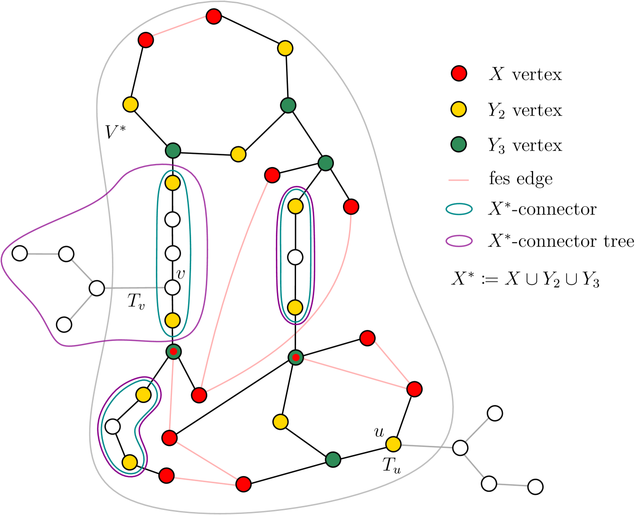
Figure 4: An illustration of the main definitions used by the FPT algorithm for parameter $\mathrm{fes}$. The grey area contains the vertices of $V^{*}$, that is, the $2$-core of $G$.

Note that $X^{*}$ contains all vertices that are part of triangles in $G[V^{*}]$ and thus in $G$. This implies that in each minimal realization of $D$, each edge incident with at least one vertex of $V\setminus X^{*}$ receives at most two labels (see Lemma˜3.1). We now formally define the above mentioned paths between the vertices of $Y_{2}$ is a more general way.

Definition 7.2.

Let $W$ with $X^{*}\subseteq W\subseteq V^{*}$ and let $P$ be a path of length at least 2 in $G[V^{*}]$ with endpoints $a$ and $b$ in $W$ and all internal vertices from $V^{*}\setminus W$. We call $P$ a $W$-connector. Moreover, let $C:=G[V(P)\cup\bigcup_{q\in V(P)\setminus\{a,b\}}V_{q}]$. We call $C$ a $W$-connector tree and the extension of $P$.

Note that the endpoints of each $X^{*}$-connector are from $Y_{2}$ and thus have degree $2$ in $G[V^{*}]$. Moreover, each internal vertex $v$ of a $W$-connector $P$ has degree exactly $2$ in $G[V^{*}]$, that is, the only two neighbors of $v$ in $G[V^{*}]$ are the predecessor and the successor of $v$ in $P$. This also implies that each endpoint of a $W$-connector has degree exactly 2 in $G[V^{*}]$. Since each edge of $P$ is incident with at least one vertex of $V\setminus W\subseteq V\setminus X^{*}$, in each minimal realization of $D$, each edge of each $W$-connector receives at most two labels (see Lemma˜3.1). The latter also holds for each $W$-connector tree.

Let $W$ with $X^{*}\subseteq W\subseteq V^{*}$ and let $q\in V\setminus(W\cup\bigcup_{w\in W}V_{w})$. There is exactly one $W$-connector tree that contains $q$.

Let $W$ with $X^{*}\subseteq W\subseteq V^{*}$. Then, there are $\mathcal{O}(|W|+\mathrm{fes})$ edges between vertices of $W$ in $G$ and there are $\mathcal{O}(|W|+\mathrm{fes})$ $W$-connectors.

Abstract Description of the Algorithm

Our algorithm uses two preprocessing steps.

In the first step, we will present a polynomial-time reduction rule based on the splitting operations presented in Section˜4. With this reduction rule, we will be able to remove vertices from pendant trees that have many vertices. After this reduction rule is applied exhaustively, for each vertex $x\in V^{*}$, the pendant tree $T_{x}$ will have $\mathcal{O}(d_{x})$ vertices, where $d_{x}$ denotes the degree of $x$ in $G[V^{*}]$.

In the second step, we extend the set $X^{*}$ to a set $W^{*}\subseteq V^{*}$ such that each $W^{*}$-connector has some useful properties (we will define connectors with these properties as nice connectors). Intuitively, a connector $P$ with extension $C$ is nice if (i) in a realization for $D$, the arcs in $D[V(C)]$ can only be realized by temporal paths that are contained in the connector tree $C$, and (ii) for each arc between a vertex outside of $C$ and a vertex inside of $C$, we can in polynomial time detect over which (unique) edge of the connector incident with one of its endpoints this arc is realized. As we will show, we can compute such a set $W^{*}$ of size $\mathcal{O}(\mathrm{fes})$ in polynomial time, or correctly detect that the input graph is not realizable. By the first part, we additionally get that the total number of vertices in pendant trees that have their root in $W^{*}$ is $\mathcal{O}(|W^{*}|+\mathrm{fes})=\mathcal{O}(\mathrm{fes})$.

The algorithm then works as follows: We iterate over all possible partial labelings $\lambda$ on the $\mathcal{O}(\mathrm{fes})$ edges incident with vertices of $W^{*}$ or vertices of pendant trees that have their root in $W^{*}$. As we will show, we can assume that each of these edges will only receive $\mathcal{O}(\mathrm{fes})$ labels in each minimal realization. For each such labeling $\lambda$, we need to check whether we can extend the labeling to the so far unlabeled edges, that is, the edges that are part of any $W^{*}$-connector. As we will show, we can compute for each such connector $P$ with extension $C$ in polynomial time a set $L_{P}$ of $\mathcal{O}(1)$ labelings for the edges of $C$, such that if $\lambda$ can be extended to a realization for $D$, then we can extend $\lambda$ (independently from the other connectors) by one of the labelings in $L_{P}$. Since $W^{*}$ has size $\mathcal{O}(\mathrm{fes})$, there are only $\mathcal{O}(\mathrm{fes})$ many $W^{*}$-connectors (see Section˜7) and for each such connector $P$, the set $L_{P}$ of labelings has constant size. Our algorithm thus iterates over all possible $\mathcal{O}(1)^{\mathcal{O}(\mathrm{fes})}=2^{\mathcal{O}(\mathrm{fes})}$ possible labeling combinations for the connectors and checks whether one of these combinations extends $\lambda$ to a realization for $D$.

Summarizing, we will show the following.

Proposition 7.3.

In polynomial time, we can detect that $D$ is not realizable, or compute a set $W^{*}$ with $X^{*}\subseteq W^{*}\subseteq V^{*}$, such that the set of edges $E^{*}$ that are (i) incident with at least one vertex of $W^{*}$ or (ii) part of some pendant tree with root in $W^{*}$, has size $\mathcal{O}(\mathrm{fes})$ and where for each labeling $\lambda$ of the edges of $E^{*}$, we can in $2^{\mathcal{O}(\mathrm{fes})}\cdot n^{\mathcal{O}(1)}$ time

• detect that there is no frugal realization for $D$ that agrees with $\lambda$ on the labels of all edges of $E^{*}$, or

• compute a labeling that realizes $D$.

The running time of this algorithm is then $\mathrm{fes}^{\mathcal{O}(\mathrm{fes}^{2})}\cdot n^{\mathcal{O}(1)}$, since (i) all preprocessing steps run in polynomial time, (ii) we only have to consider $\mathrm{fes}^{\mathcal{O}(\mathrm{fes}^{2})}$ labelings $\lambda$ (since we prelabel $\mathcal{O}(\mathrm{fes})$ edges with $\mathcal{O}(\mathrm{fes})$ labels each), and (iii) for each labeling $\lambda$, we only have to check for $2^{\mathcal{O}(\mathrm{fes})}$ possible ways to extend $\lambda$ to a realization for $D$. To see the second part, we show that it is sufficient to assign only labels of $\{i\cdot 2\cdot n\mid i\in\mathcal{O}(\mathrm{fes}^{2})\}$ in $\lambda$.

To describe our algorithm, we will use the notion of “merging” several partial labelings. This is formally defined as follows.

Definition 7.4.

Let $E_{1}$ and $E_{2}$ be (not necessarily disjoint) subsets of $E$. For $\lambda_{1}\colon E_{1}\to 2^{\mathbb{N}}$ and $\lambda_{2}\colon E_{2}\to 2^{\mathbb{N}}$, we define the labeling $\lambda_{1}\ltimes\lambda_{2}\colon E_{1}\cup E_{2}\to 2^{\mathbb{N}}$ by $(\lambda_{1}\ltimes\lambda_{2})(e):=\lambda_{2}(e)$ if $e\in E_{2}$ and $(\lambda_{1}\ltimes\lambda_{2})(e):=\lambda_{1}(e)$ otherwise.

7.1 Independent structural implication

In our algorithm, we will enumerate all reasonable prelabelings of a set of $\mathcal{O}(\mathrm{fes})$ edges. To ensure that this enumeration can be done in FPT-time for $\mathrm{fes}$, we need to ensure that ’few’ labels per edges are sufficient. The following result ensures this property, but is also of independent interest for the understanding of our problem.

Theorem 7.5.

Let $D$ be an instance of URGR with solid graph $G$. In each minimal realization of $D$, each edge of $G$ receives $\mathcal{O}(\mathrm{fes})$ labels.

Proof 7.6.

Let $\lambda$ be a realization of $D$. Let $F$ be a feedback edge set of $G$ of size $\mathrm{fes}$. Moreover, let $V^{*}$ and $X^{*}$ be defined as above based on $F$ and recall that $|X^{*}|\in\mathcal{O}(|F|)=\mathcal{O}(\mathrm{fes})$. If each edge receives $\mathcal{O}(\mathrm{fes})$ labels, we are done. So assume that there is an edge $e$ that receives $\omega(\mathrm{fes})$ labels. We will show that $\lambda$ is not a minimal realization for $D$. Note that if not both endpoints of $e$ are in $X^{*}$, then $e$ is not part of a triangle in $G$, which implies that $\lambda$ is not a minimal realization, since in each such realization, $e$ would receive at most two labels (see Lemma˜3.1). Thus, assume in the following that both endpoints of $e$ are from $X^{*}$.

Similar to the proof of Lemma˜3.3, we denote for each vertex $v\in V$ with $\alpha_{v}$ the smallest label assigned to $e$ for which there is a temporal path under $\lambda$ that starts in $v$ and traverses $e$ at time $\alpha_{v}$, if such a label exists. Let $L_{e}:=\{\alpha_{v}\mid v\in V,\alpha_{v}\text{ exists}\}$. Note that if there is at least one label $\ell$ assigned to $e$ that is not contained in $L_{e}$, then removing label $\ell$ from $e$ still preserves at least one temporal path between any two vertices for which a temporal path exists under $\lambda$. Consequently, if such a label $\ell$ exists, we can immediately conclude that $\lambda$ is not a minimal realization for $D$. Recall that $e$ receives $\omega(\mathrm{fes})$ labels. Hence, to show that $\lambda$ is not a minimal realization, it suffices to show that $L_{e}$ has size $\mathcal{O}(\mathrm{fes})$.

To this end, note that each vertex of $V$ is (a) a vertex of $X^{*}$, (b) contained in some $X^{*}$-connector tree $C$ (excluding the two vertices of $C$ in $X^{*}$), or (c) a vertex of some pendant tree rooted in $X^{*}$ (excluding the root).

Since $X^{*}$ has size $\mathcal{O}(\mathrm{fes})$, the vertices of $X^{*}$ contribute $\mathcal{O}(\mathrm{fes})$ different labels to $L_{e}$.

Let $C$ be a $X^{*}$-connector tree where $a$ and $b$ are the two unique vertices of $X^{*}$ in $C$. By definition of connector trees, $a$ and $b$ are both leaves in $C$. Moreover, since these vertices are the only vertices of $X^{*}$ in $C$ and both endpoints of $e$ are from $X^{*}$, each temporal path starting in $C$ and traversing edge $e$ has to leave the connector tree via the unique edge $\{a,a^{\prime}\}$ incident with $a$ in $C$ or via the unique edge $\{b,b^{\prime}\}$ incident with $b$ in $C$. Since both edges are not part of a triangle, they both receive at most two labels each under $\lambda$, or $\lambda$ is not a minimal realization for $D$ (see Lemma˜3.1). Thus, assume that both edges receive at most two labels each. Hence, all vertices of $V(C)\setminus\{a,b\}$ contribute in total at most four labels to $L_{e}$. Since there are $\mathcal{O}(\mathrm{fes})$ $X^{*}$-connectors (see Section˜7), all vertices that are contained in $X^{*}$-connectors thus contribute $\mathcal{O}(\mathrm{fes})$ labels in total to $L_{e}$.

To show that $L_{e}$ has size $\mathcal{O}(\mathrm{fes})$, it suffices to show that all vertices that are contained in pendant trees with roots in $X^{*}$ contribute $\mathcal{O}(\mathrm{fes})$ labels in total to $L_{e}$. Let $x\in X^{*}$. We show that all vertices of $T_{x}$ contribute $\mathcal{O}(d_{x})$ labels in total to $L_{e}$, where $d_{x}$ denotes the degree of $x$ in $G[V^{*}]$. Let $v\in V_{x}$ and let $P$ be a temporal path from $v$ that traverses the edge $e$ at time $\alpha_{v}$. Note that $P$ traverses one edge $e_{1}$ incident with $x$ in $T_{x}$ and then traverses an edge $e_{2}$ between $x$ and some other vertex of $V^{*}$. Since $e_{1}$ is an edge of $T_{x}$, $e_{1}$ is a bridge in $G$, which implies that $\max\lambda(e_{1})\leq\min\lambda(e_{2})$. Hence, we can assume that $P$ either traverses the edge $e_{2}$ at time $\min\lambda(e_{2})$ or at time $\min(\lambda(e_{2})\setminus\min\lambda(e_{2}))$ (if $e_{2}$ receives at least two labels). Thus, for each edge between $x$ and some other vertex of $V^{*}$, at most two labels are used that define the $\alpha_{v}$ values for the vertices $v\in V_{x}$. This implies that the vertices of $T_{x}$ contribute $\mathcal{O}(d_{x})$ labels in total to $L_{e}$. Note that Section˜7 implies that the sum of degrees of all vertices of $X^{*}$ in $G[V^{*}]$ is $\mathcal{O}(\mathrm{fes})$. Hence, all vertices that are contained in pendant trees with roots in $X^{*}$ contribute $\mathcal{O}(\mathrm{fes})$ labels in total to $L_{e}$.

Consequently, $L_{e}$ has size $\mathcal{O}(\mathrm{fes})$. This implies that $\lambda$ is not a minimal realization, since $e$ receives $\omega(\mathrm{fes})$ labels under $\lambda$.

7.2 Dealing with the pendant trees

Our goal in this subsection is to prove the following.

Proposition 7.7.

In polynomial time, we can (i) detect that $D$ is not realizable or (ii) obtain an equivalent instance by (a) adding polynomially many degree-1 vertices to $D$ and (b) removing vertices from $D$, such that in the resulting instance, in each pendant tree $T_{v}$ for $v\in V^{*}$, $\mathcal{O}(d_{v})$ vertices remain, where $d_{v}$ denotes the degree of $v$ in $G[V^{*}]$.

For each vertex $v\in V^{*}$, let $B_{v}$ denote the vertices of $T_{v}$ that are adjacent to $v$ in $G$. By definition of $T_{v}$, for each vertex $b\in B_{v}$, the edge $\{v,b\}$ is a bridge in $G$. We call $B_{v}$ the bridge vertices of $T_{v}$.

For each vertex $v\in V^{*}$, apply the operations behind Lemma˜4.12, Lemma˜4.15, and Lemma˜4.17 to each bridge between $v$ and $B_{v}$. These operations might possibly detect that $D$ is not realizable. In this case, report that $D$ is not realizable. Otherwise, each such operation individually splits our instance into at most two instances. Moreover, at most one of these instances contains cycles, since each bridge in $T_{v}$ has a tree on one side. For all resulting tree instances, we check in polynomial time whether they are realizable. If at least one is not realizable, we correctly output that $D$ is not realizable. Otherwise, we only (again) remain with one instance, and this instance contains cycles. In particular, this instance is (besides some possible degree-1 vertices) a subgraph of $D[V^{*}\cup N(V^{*})]$. For convenience, assume that $D$ already is the unique resulting instance. Note that $G[\{v\}\cup B_{v}]$ is an induced star with center $v$, where each edge between $v$ and a vertex of $B_{v}$ is a bridge in $G$. Hence, with the same arguments behind Lemma˜5.4, $D$ is not realizable if $D[B_{v}]$ is not a complete DAG, since the operations behind Lemma˜4.12 and Lemma˜4.17 were applied on all bridges between $v$ and $B_{v}$. Hence, if $D[B_{v}]$ is not a complete DAG, we correctly output that $D$ is not realizable. Otherwise, we continue with the knowledge that $D[B_{v}]$ is a complete DAG. This complete DAG $D[B_{v}]$ thus implies a unique total order on the vertices of $B_{v}$ starting from the unique source in $D[B_{v}]$. In the following, we denote the $i$th vertex of this total order of $B_{v}$ by $b_{v}^{i}$. Consequently, for each $1\leq i<j\leq|B_{v}|$, $(b_{v}^{i},b_{v}^{j})\in A$.

Additionally, we check for any two adjacent bridges $e$ and $e^{\prime}$ whether they are both bundled and separated. If this is the case for any pair of adjacent bridges, we can correctly detect that $D$ is not realizable due to Corollary˜4.11. Since this property can be checked in polynomial time, we assume in the following that no pair of adjacent bridges is both bundled and separated.

We now observe a necessary property for realizable instances.

Lemma 7.8.

Let $v\in V^{*}$ and let $u\in V\setminus(\{v\}\cup V_{v})$. If $D$ is realizable, then the set $[1,|B_{v}|]$ can be partitioned in three consecutive and pairwise disjoint (possibly empty) intervals $I_{1}$, $I_{2}$, and $I_{3}$, such that

• $(b_{v}^{i},u)\in A$ and $(u,b_{v}^{i})\notin A$ for each $i\in I_{1}$,

• $(b_{v}^{i},u)\notin A$ and $(u,b_{v}^{i})\notin A$ for each $i\in I_{2}$, and

• $(u,b_{v}^{i})\in A$ and $(b_{v}^{i},u)\notin A$ for each $i\in I_{3}$.

Proof 7.9.

Since $u\in V\setminus(\{v\}\cup V_{v})$, for each $b_{v}^{i}\in B_{v}$, $A$ contains at most one of the arcs $(u,b_{v}^{i})$ and $(b_{v}^{i},u)$. Let $\lambda$ be a realization of $D$.

If $(b_{v}^{i},u)\in A$ for some $i\in[2,|B_{v}|]$, then there is a temporal $(b_{v}^{i},u)$-path under $\lambda$. This temporal path starts by traversing the edge $\{b_{v}^{i},v\}$ at time at least $\min\lambda(\{b_{v}^{i},v\})$. Since for each $j\in[1,i-1]$, $A$ contains the arc $(b_{v}^{j},b_{v}^{i})$, $\min\lambda(\{b_{v}^{j},v\})\leq\min\lambda(\{b_{v}^{i},v\})$. Hence, there is also a temporal $(b_{v}^{j},u)$-path under $\lambda$. This implies that $(b_{v}^{j},u)\in A$. Moreover, this implies that the interval $I_{1}$ exists as stated and extends from the start of $B_{v}$ (ending with the largest $i$ for which $(b_{v}^{i},u)\in A$).

Similarly, if $(u,b_{v}^{i})\in A$ for some $i\in[1,|B_{v}|-1]$, then there is a temporal $(u,b_{v}^{i})$-path under $\lambda$. This temporal path ends by traversing the edge $\{v,b_{v}^{i}\}$ at time at most $\max\lambda(\{v,b_{v}^{i}\})$. Since for each $j\in[i+1,|B_{v}|]$, $A$ contains the arc $(b_{v}^{i},b_{v}^{j})$, $\min\lambda(\{v,b_{v}^{j}\})\geq\max\lambda(\{v,b_{v}^{i}\})$. Hence, there is also a temporal $(u,b_{v}^{j})$-path under $\lambda$. This implies that $(u,b_{v}^{j})\in A$. Moreover, this implies that the interval $I_{3}$ exists as stated and extends to the end of $B_{v}$ (starting from the smallest $i$ for which $(b_{v}^{i},u)\in A$).

Consequently, the interval $I_{2}$ contains the remaining vertices of $B_{v}$. None of the vertices of $I_{2}$ can have an arc from or towards $u$ as otherwise, one of the other two intervals could be extended.

Note that this property can be checked for each pair of vertices $v$ and $u$ in polynomial time. Hence, if the property does not hold for some vertex pair, we correctly output that $D$ is not realizable. In the remainder, assume that these intervals exist for each pair of vertices $v$ and $u$. Moreover, note that they can be computed in polynomial time. We may call the interval $I_{2}$ the middle interval of $u$ with respect to $T_{v}$.

Based on these intervals, we now define for each vertex $v\in V^{*}$ and each neighbor $u$ of $v$ in $V^{*}$ a set of $\mathcal{O}(1)$ edges in $T_{v}$ that ’surround’ the edge $\{u,v\}$. Intuitively, these edges will be the only edges that can possibly share a label with $\{u,v\}$ in any realization of $G$.

Definition 7.10.

Let $e:=\{u,v\}\subseteq V^{*}$ with $e\in E$, and let $B_{v}$ denote the bridge vertices of $T_{v}$. Moreover, let $I_{2}$ denote the middle interval of $u$ with respect to $T_{v}$ according to Lemma˜7.8. If $B_{v}\neq\emptyset$, we define the edges of $T_{v}$ that surround $e$ as:

• $\{\{v,b_{v}^{j}\}\mid j\in[i-2,i+2]\cap[1,|B_{v}|]\}$, if the interval $I_{2}$ has size at most one, where $i\in[1,|B_{v}|]$ is the smallest index, such that $(b_{v}^{j},u)\in A$ for each $1\leq j<i$ and $(u,b_{v}^{k})\in A$ for each $i<k\leq|B_{v}|$, and as

• $\emptyset$, otherwise.

In the latter case, we say that the edges $\{b_{v}^{j},v\}$ and $\{b_{v}^{k},v\}$ block the edge $e$, where $j=\min I_{2}$ and $k=\max I_{2}$.

We now show that this definition matches the previous intuition.

Lemma 7.11.

Let $e:=\{u,v\}\subseteq V^{*}$ with $e\in E$, and let $S$ denote the edges of $T_{v}$ that surround $e$. Then, in each realization of $D$, $e$ shares no label with any edge of $T_{v}$ that is incident with $v$ and not in $S$. Moreover, for each $i\in[1,|B_{v}|-1]$ where $\{v,b_{v}^{i}\}$ and $\{v,b_{v}^{i+1}\}$ are not in $S$, in each frugal realization $\lambda$ of $D$, $\lambda(e)\cap[\min\lambda(\{v,b_{v}^{i}\}),\max\lambda(\{v,b_{v}^{i+1}\})]=\emptyset$.

Proof 7.12.

Recall that each bridge $e$ of $G$ receives at least one label in each realization of $D$. Let $B_{v}$ be the bridge vertices of $T_{v}$. Recall that $D[B_{v}]$ is a complete DAG. This implies that for each realization $\lambda$ for $D$ and for each two $b_{v}^{k}$ and $b_{v}^{\ell}$ from $B_{v}$ with $k<\ell$, $\min\lambda(\{v,b_{v}^{k}\})<\max\lambda(\{v,b_{v}^{\ell}\})$ and $\max\lambda(\{v,b_{v}^{k}\})\leq\min\lambda(\{v,b_{v}^{\ell}\})$.

We distinguish two case.

Case 1: $S=\emptyset$. That is, there is some $i\in[1,|B_{v}|-1]$, such that there is no arc between $u$ and any vertex of $\{b_{v}^{i},b_{v}^{i+1}\}$. Let $\lambda$ be a realization for $D$. We show that $\lambda(e)=\emptyset$. Assume towards a contradiction that $\lambda(e)\neq\emptyset$. Since there is no arc between $u$ and $b_{v}^{i}$, Section˜2 implies that there is some $\alpha\in\mathbb{N}$, such that $\lambda(e)=\lambda(\{v,b_{v}^{i}\})=\{\alpha\}$. Since $(b_{v}^{i},b_{v}^{i+1})\in A$, $\max\lambda(\{v,b_{v}^{i+1}\})>\min\lambda(\{v,b_{v}^{i}\})=\alpha$. Thus, $(u,v,b_{v}^{i+1})$ is a temporal path under $\lambda$. This contradicts the fact that $\lambda$ realizes $D$, since $(u,b_{v}^{i+1})$ is not an arc of $D$. Hence, the statement holds if $S=\emptyset$.

Case 2: $S\neq\emptyset$. Assume towards a contradiction that $e$ shares a label with at least one edge $\{v,b_{v}^{j}\}$ of $T_{v}$ that is incident with $v$ and does not surround $e$. Let $i\in[1,|B_{v}|]$ be the index over which $S$ was defined. We distinguish two subcases.

Case 2.1: $j<i$. By definition $\{\{v,b_{v}^{\ell}\}\mid\ell\in\{i-2,i-1,i\}\}\subseteq S$. Hence, $j\leq i-3$. By choice of $i$, $(b_{v}^{i-1},u)\in A$. Hence, $\max\lambda(\{v,b_{v}^{i-1}\})\leq\min\lambda(e)\leq\max\lambda(e)$. By the initial argumentation, this implies that $\max\lambda(\{v,b_{v}^{j}\})\leq\min\lambda(\{v,b_{v}^{i-2}\})<\max\lambda(\{v,b_{v}^{i-1}\})\leq\min\lambda(e)$. This contradicts the assumption that $e$ shares a label with $\{v,b_{v}^{j}\}$.

Case 2.2: $j>i$. This case can be shown analogously.

Consequently, no edge of $T_{v}$ incident with $v$ outside of $S$ shares a label with $e$. We now show the second part of the statement. That is, let $i\in[1,|B_{v}|-1]$ where both $e_{i}:=\{v,b_{v}^{i}\}$ and $e_{i+1}:=\{v,b_{v}^{i+1}\}$ are not in $S$, we show that $e$ has no label from $[\min\lambda(e_{i}),\max\lambda(e_{i+1})]$. Assume towards a contradiction that this is not the case. By the above, we know that $\lambda(e)\cap(\lambda(e_{i})\cup\lambda(e_{i+1}))=\emptyset$. Moreover, $e$ cannot have a label between $\min\lambda(e_{i})$ and $\max\lambda(e_{i})$, as otherwise, a solid edge between $u$ and $b_{v}^{i}$ would be realized. Similarly, $e$ cannot have a label between $\min\lambda(e_{i+1})$ and $\max\lambda(e_{i+1})$. Hence, the only remaining option is that $e$ receives a label strictly between $\max\lambda(e_{i})$ and $\min\lambda(e_{i+1})$. This then implies that the arcs $(b_{v}^{i},u)$ and $(u,b_{v}^{i+1})$ are realized. Hence, $b_{v}^{i}$ ($b_{v}^{i+1}$) is from the interval $I_{1}$ ($I_{3}$) of $u$ with respect to the pendant tree $T_{v}$ according to Lemma˜7.8. By definition of $S$, both $e_{i}$ and $e_{i+1}$ are in $S$; a contradiction.

Based on this insight about surrounding edges, we now define another sanity check. This will then ensure that we can assume some consistent reachabilities between vertices outside of $T_{v}$ and bridge vertices that are in $T_{v}$ but that do not surround any external edge. The sanity check reads as follows.

Lemma 7.13.

Let $v\in V^{*}$ with $|B_{v}|\geq 3$ and let $i\in[1,|B_{v}|-1]$ such that neither edge $\{b_{v}^{i},v\}$ nor edge $\{b_{v}^{i+1},v\}$ is surrounding or blocking any edge incident with $v$ that is outside of $T_{v}$. If $D$ is realizable, then for each vertex $x\in V\setminus(\{v\}\cup V_{v})$

• $D_{xb_{v}^{i}}=D_{xb_{v}^{i+1}}$ (and $D_{xb_{v}^{i+1}}=D_{x\,\mathrm{out}_{v}^{i+1}}$, where $\mathrm{out}_{v}^{i+1}$ is the out-leaf of $b_{v}^{i+1}$, if it exists), and

• $D_{b_{v}^{i}x}=D_{b_{v}^{i+1}x}$ (and $D_{b_{v}^{i}x}=D_{\mathrm{in}_{v}^{i}x}$, where $\mathrm{in}_{v}^{i}$ is the in-leaf of $b_{v}^{i}$, if it exists).

Proof 7.14.

Let $\lambda$ be a realization for $D$ and let $x\in V\setminus(\{v\}\cup V_{v})$. Moreover, let $\alpha$ be the smallest label such that there is a temporal $(x,v)$-path $P$ under $\lambda$ that reaches $v$ at time $\alpha$. Since $x\notin V\setminus(\{v\}\cup V_{v})$, the path $P$ traverses an edge $e$ between $v$ and some other vertex of $V^{*}$ at time $\alpha$. Since neither edge $\{b_{v}^{i},v\}$ nor edge $\{b_{v}^{i+1},v\}$ is surrounding $e$, Lemma˜7.11 implies that $\alpha<\min\lambda(\{b_{v}^{i},v\})$ or $\alpha>\max\lambda(\{b_{v}^{i+1},v\})$. If $\alpha<\min\lambda(\{b_{v}^{i},v\})$, $P$ can be extended to reach the vertices $b_{v}^{i}$, $b_{v}^{i+1}$, and $\mathrm{out}^{i+1}$ (if the latter exists). In this case, $D_{xb_{v}^{i}}=D_{xb_{v}^{i+1}}=D_{x\,\mathrm{out}_{v}^{i+1}}=1$. Otherwise, that is, if $\alpha>\max\lambda(\{b_{v}^{i+1},v\})$ , $x$ can reach none of $b_{v}^{i}$, $b_{v}^{i+1}$, and $\mathrm{out}^{i+1}$. In this case, $D_{xb_{v}^{i}}=D_{xb_{v}^{i+1}}=D_{x\,\mathrm{out}_{v}^{i+1}}=0$.

The reachability towards $x$ can be shown analogously.

This property can be checked for each vertex $v\in V^{*}$ and each $b_{v}^{i}\in V_{v}$ in polynomial time. If the property does not hold for some vertex pair, we correctly output that $D$ is not realizable. In the remainder, thus assume that the property holds for all vertex pairs.

Based on this sanity check, we now define our final reduction rule to reduce the size of pendant trees.

Lemma 7.15.

Let $v\in V^{*}$ and let $b_{v}^{i}\in B_{v}$ with $6\leq i\leq|B_{v}|-5$, such that none of the edges $\{\{v,b_{v}^{j}\}\mid i-5\leq j\leq i+5\}$ is surrounding or blocking any edge $e$ incident with $v$ and some other vertex of $V^{*}$. Then, $D$ is realizable if and only if (i) $D[V(T_{v})]=D[\{v\}\cup V_{v}]$ is realizable and (ii) $D^{\prime}$ is realizable, where $D^{\prime}$ is the instance obtained from $D$ by removing $b_{v}^{i}$ and its potential in- and out-leaf.

Proof 7.16.

Let $D^{\prime}$ be the resulting instance with solid graph $G^{\prime}$ after removing $b_{v}^{i}$ and its possible leaf-neighbors form $D$. Let $D_{v}:=D[V(T_{v})]=D[\{v\}\cup V_{v}]$. Moreover, for each $j\in[1,|B_{v}|]$, let $e_{i}$ denote the bridge $\{b_{v}^{i},v\}$.

The first direction of the statement follows immediately: Let $\lambda$ be a realization for $D$. Then, the restriction of $\lambda$ to the edges of $G^{\prime}$ realizes $D^{\prime}$, since no path in $G$ between any two vertices of $G^{\prime}$ uses vertices that are removed from $G$. Similarly, the restriction of $\lambda$ to the edges of $T_{v}$ realizes $D_{v}$, since no path in $G$ between any two vertices of $T_{v}$ uses vertices outside of $T_{v}$. Hence, if $D$ is realizable, then both $D^{\prime}$ and $D_{v}$ are realizable.

So consider the second direction. Let $\lambda^{\prime}$ be a frugal realization for $D^{\prime}$ and let $\lambda_{v}$ be a frugal realization for $D_{v}$. We show that there is a realization $\lambda$ for $D$. To this end, we will combine both realizations for $D^{\prime}$ and $D_{v}$.

Recall that $e_{i}$ is not an edge that surrounds or blocks any external edge incident with $v$. Note that for each external edge $e$ incident with $v$, in both $D$ and $D^{\prime}$ the same edges in $T_{v}$ are surrounding $e$. If $e$ is surrounded by at least one edge in $T_{v}$ under $D$, then this trivially follows by definition of surrounding edges. Otherwise, if no edge surrounds $e$ under $D$, then, since $e_{i}$ is not an edge blocking $e$, $D^{\prime}$ still contains both edges that block $e$ in $D$. Based on these two edges, no edge surrounds $e$ under $D^{\prime}$. Due to Lemma˜7.11, this implies that for each external edge $e$ incident with $v$, $e$ receives no label in $[\min\lambda^{\prime}(e_{i-5}),\max\lambda^{\prime}(e_{i+5})]$.

Let $s=i-3$ if $e_{i-3}$ is a special bridge in $D$, and let $s=i-4$, otherwise. Similarly, let $t=i+3$ if $e_{i+3}$ is a special bridge in $D$, and let $t=i+4$, otherwise. The choice of $s$ and $t$ is important to ensure that the edges $e_{s-1}$ ($e_{t-1}$) and $e_{s+1}$ ($e_{t+1}$) are separated under $D$, $D^{\prime}$, and $D_{v}$. We will show that this property holds when providing a realization for $D$. Before we can define a realization for $D$, we observe several properties about the edges $e_{s}$ and $e_{t}$.

Let $j\in[1,s]\cup[t,|B_{v}|]$. Observe that $e_{j}$ and $e_{i}$ are separated under $D$. This implies that $e_{j}$ and $e_{i}$ are not bundled under $D$, since we would have already detected that $D$ is a no-instance if $e_{j}$ and $e_{i}$ are both bundled and separated under $D$ (see Corollary˜4.11). Hence, the removal of $b_{v}^{i}$ and its possible leaves did not make $e_{j}$ non-special, if $e_{j}$ was special in $D$. In other words, $e_{j}$ is special in $D$ if and only if $e_{j}$ is special in $D^{\prime}$.

Let $j\in[s,t]$. Since $e_{j}$ does not surround any external edge incident with $v$, $e_{j}$ is special in $D$ if and only if $e_{j}$ is special in $D_{v}$. This is due to the fact that $e_{j}$ cannot share a label with any external edge incident with $v$ (see Lemma˜7.11).

This in particular implies that $e_{s}$ ($e_{t}$) is special in $D^{\prime}$ if an only if $e_{s}$ ($e_{t}$) is special in $D_{v}$. Moreover, $\max\lambda_{v}(e_{s})<\min\lambda_{v}(e_{t})$, since $e_{s}$ and $e_{t}$ are separated under $D_{v}$. Similarly, $\max\lambda^{\prime}(e_{s})<\min\lambda^{\prime}(e_{t})$, since $e_{s}$ and $e_{t}$ are separated under $D^{\prime}$. We can thus assume without loss of generality that $\lambda^{\prime}(e_{s})=\lambda_{v}(e_{s})$ and $\lambda^{\prime}(e_{t})=\lambda_{v}(e_{t})$ (by introducing arbitrarily many empty snapshots in both labelings).

Based on this property, we now define a realization $\lambda$ for $D$. The labeling $\lambda$ agrees with $\lambda_{v}$ on all edges incident with at least one vertex of $\{b_{v}^{j}\mid j\in[s+1,t-1]\}$, and agrees with $\lambda^{\prime}$ on all other edges. We show that $\lambda$ realizes $D$. Let $W$ contain the vertices $b_{v}^{j}$ with $j\in[s+1,t-1]$ and their possible leaves. Since paths between any two vertices of $V\setminus W$ only use vertices outside of $W$, and $\lambda^{\prime}$ realizes $D^{\prime}$, exactly the arcs of $D$ between vertices of $V\setminus W$ are realized by $\lambda$. Similarly, paths between vertices of $W$ only use vertices of $W\cup\{v\}$, since all vertices of $W$ are in $T_{v}$. Since $\lambda$ agrees with $\lambda_{v}$ on all edges incident with at least one vertex of $W$ and $\lambda_{v}$ realized $D_{v}$, exactly the arcs of $D$ between vertices of $W$ are realized by $\lambda$.

It thus remains to show that exactly the arcs of $D$ between vertices of $W$ and vertices of $V\setminus W$ are realized by $\lambda$.

Let $x\in V\setminus(\{v\}\cup V_{v})$ and let $j\in[s,t]$. Then, since we assumed that the property of Lemma˜7.13 holds (as otherwise we already detected that $D$ is not realizable), $D_{xb_{v}^{j}}=D_{xb_{v}^{s-1}}$ (and $D_{x\,\mathrm{out}^{j}}=D_{xb_{v}^{s-1}}$ if the out-leaf $\mathrm{out}^{j}$ of $b_{v}^{j}$ exists). Since $\lambda^{\prime}$ realizes $D^{\prime}$, if $D_{xb_{v}^{s-1}}=1$, then there is a temporal $(x,b_{v}^{s-1})$-path $P$ under $\lambda^{\prime}$ (and thus under $\lambda$). The path $P$ traverses the edge $e_{s-1}$ at time at most $\max\lambda^{\prime}(e_{s-1})=\max\lambda(e_{s-1})<\min\lambda(e_{j})$. This implies that there is also a temporal $(x,b_{v}^{j})$-path (and a temporal $(x,\mathrm{out}^{j})$-path, if $\mathrm{out}^{j}$ exists) under $\lambda$. Similarly, if $D_{xb_{v}^{s-1}}=0$, then there is no temporal $(x,b_{v}^{s-1})$-path under $\lambda^{\prime}$ (and thus also not under $\lambda$). In particular, each temporal $(x,v)$-path under $\lambda$ reaches $v$ at time at least $\min\lambda(e_{s-1})$. As initially discussed, no external edge incident with $v$ has a label in $[\min\lambda^{\prime}(e_{s-1}),\max\lambda^{\prime}(e_{t+1})]$. Hence, each temporal $(x,v)$-path under $\lambda$ reaches $v$ at time larger than $\max\lambda(e_{t+1})>\max\lambda(e_{j})$. This implies that there is also no temporal $(x,b_{v}^{j})$-path (and no temporal $(x,\mathrm{out}^{j})$-path, if $\mathrm{out}^{j}$ exists) under $\lambda$.

Hence, the possible arcs from $x$ to $b_{v}^{j}$ and $\mathrm{out}^{j}$ are realized by $\lambda$ if and only if they exist. Similarly, the possible arcs from $b_{v}^{j}$ and $\mathrm{in}^{j}$ to $x$ are realized if and only if they exist.

It thus remains to consider reachability between vertices of $W$ and vertices of $V_{v}\setminus W$. To analyze this case, we finally show the reason why we chose the specific values for $s$ and $t$. We show that in both $D^{\prime}$ and $D_{v}$, $e_{s-1}$ and $e_{s+1}$ are separated. This is due to the fact that (i) if $s=i-3$, then $e_{i-3}$ is special which implies that $e_{s-1}$ and $e_{s+1}$ are separated, and (ii) if $s=i-4$, then $e_{i-3}$ is non-special which implies that $e_{s-1}$ and $e_{s+1}$ are separated. By the earlier argumentation, $e_{s}$ is special under either all or none of the graphs $D$, $D^{\prime}$, and $D_{v}$. Thus, each temporal path that traverses first an edge in $T_{v}$ not incident with a vertex in $W$ and afterwards an edge incident with a vertex of $W$ exists under $\lambda_{v}$ if and only if it exists under $\lambda$. This implies that $\lambda$ realizes exactly the arcs between the vertices of $T_{v}$, since $\lambda_{v}$ realizes $D_{v}$.

In conclusion, $\lambda$ realizes $D$.

Note that this implies that we can in polynomial time (correctly detect that $D$ is not realizable or) reduce the size of each fixed pendant tree $T_{x}$ with $x\in V^{*}$ to a size of $\mathcal{O}(d_{x})$, where $d_{x}$ denotes the degree of $x$ in $G[V^{*}]$. This is due to the fact that each of the $\mathcal{O}(d_{x})$ edges defines at most $5$ surrounding or blocking edges in $T_{x}$, and we can remove neighbors of $x$ in $T_{x}$ if there are more than 11 consecutive (with respect to the topological order on $B_{x}$) bridges incident with $x$ that are all not surrounding or blocking any external edge. This thus proves Proposition˜7.7.

7.3 Ensuring connectors with nice properties

In this section we show how to extend the vertex set $X^{*}$ to a set $W^{*}$ of size $\mathcal{O}(\mathrm{fes})$, such that each $W^{*}$-connector has some useful properties that we will use in our algorithm.

To define these useful properties, we distinguish between several types of connectors.

Definition 7.17.

Let $W$ with $X^{*}\subseteq W\subseteq V^{*}$ and let $P$ be a $W$-connector with endpoints $a$ and $b$ from $V^{*}$. We say that $P$ is trivial if $P$ has length at most $3$. Otherwise, let $a^{\prime}$ be the successor of $a$ in $P$ and let $a^{\prime\prime}$ be the successor of $a^{\prime}$ in $P$. Similarly, let $b^{\prime}$ be the predecessor of $b$ in $P$ and let $b^{\prime\prime}$ be the predecessor of $b^{\prime}$ in $P$. We say that $P$ is an (in,out)-connector if $(a,a^{\prime\prime})\in A$ and $(b^{\prime\prime},b)\in A$. Moreover, $P$ a dense (in,out)-connector, if the path $P$ is a dense path in $D$ and $P$ is an (in,out)-connector.

Robust Connectors

The first property we consider are robust connectors, which are defined as follows.

Definition 7.18.

Let $W$ with $X^{*}\subseteq W\subseteq V^{*}$ and let $P$ be a $W$-connector with endpoints $a$ and $b$ and extension $C$. We say that $P$ is robust if there is no dense path between $a$ and $b$ outside of $C$, that is, if there is no dense path from $a$ to $b$ in $D[V\setminus(V(C)\setminus\{a,b\})]$ and there is no dense path from $b$ to $a$ in $D[V\setminus(V(C)\setminus\{a,b\})]$.

In other words, in a robust connector $P$, the reachability between the vertices of the extension of $P$ has to be achieved via temporal paths that only use subpaths of the extension $C$ of $P$.

Let $W$ with $X^{*}\subseteq W\subseteq V^{*}$ and let $P$ be a robust $W$-connector with extension $C$. Then, for each realization $\lambda^{*}$ of $D$, $\lambda^{*}_{C}$ realizes $D[V(C)]$, where $\lambda^{*}_{C}$ is the restriction of $\lambda^{*}$ to the edges of $C$.

This then directly implies the following for robust connectors.

Let $W$ with $X^{*}\subseteq W\subseteq V^{*}$ and let $P$ be a robust $W$-connector. Then for each arc $(q,q^{\prime})\in A$ with $q,q^{\prime}\in V(P)$, the subpath of $P$ from $q$ to $q^{\prime}$ is dense or $D$ is not realizable.

Additionally, we observe the following hereditary property for robust connectors.

Let $W$ and $W^{\prime}$ with $X^{*}\subseteq W\subseteq W^{\prime}\subseteq V^{*}$. Moreover, let $P$ be a $W$-connector and let $P^{\prime}$ be a $W^{\prime}$-connector such that $P^{\prime}$ is a subpath of $P$. Then, $P^{\prime}$ is robust if $P$ is robust.

Finally, since the definition of robust connectors only depends on the non-existence of paths between the endpoints that are outside of the connector, a connector $P$ remains robust, even if adding vertices outside of $P$ to $W$. Formally, this reads as follows.

Let $W$ and $W^{\prime}$ with $X^{*}\subseteq W\subseteq W^{\prime}\subseteq V^{*}$. Moreover, let $P$ be a path in $G[V^{*}]$, such that $P$ is both a $W$-connector and a $W^{\prime}$-connector. Then, $P$ is a robust $W$-connector if and only if $P$ is a robust $W^{\prime}$-connector.

Based on these properties, we now show that we can find a constant number of vertices of a given connector $P$ to add to $W$ to ensure that each resulting subconnector is robust or trivial.

Lemma 7.19.

Let $W$ with $X^{*}\subseteq W\subseteq V^{*}$ and let $P$ be a non-trivial $W$-connector. Then, we can compute in polynomial time a set $U_{P}\subseteq V(P)$ of size at most $6$, such that (i) there are at most two $(W\cup U_{P})$-connectors which are subpaths of $P$ and (ii) each $(W\cup U_{P})$-connector which is a subpath of $P$ is trivial or robust.

Proof 7.20.

Let $a,a^{\prime},a^{\prime\prime}$ be the first three vertices of $P$ and let $b^{\prime\prime},b^{\prime},b$ be the last three vertices of $P$. We distinguish two cases.

Case 1: $P$ is not an (in,out)-connector. We set $U_{P}:=\{a^{\prime},a^{\prime\prime},b^{\prime},b^{\prime\prime}\}$. Clearly, there is at most one $(W\cup U_{P})$-connector which is a subpath of $P$, namely the subpath $P^{\prime}$ of $P$ from $a^{\prime\prime}$ to $b^{\prime\prime}$. Assume towards a contradiction that $P^{\prime}$ is not robust. This implies that there is a dense path $R$ in $D$ between $a^{\prime\prime}$ and $b^{\prime\prime}$ that uses no edge of $P^{\prime}$. Assume without loss of generality that $R$ goes from $a^{\prime\prime}$ to $b^{\prime\prime}$. Note that the dense path $R$ has to visit both $a$ and $b$. This implies that $(a^{\prime\prime},a)\in A$ and $(b,b^{\prime\prime})\in A$; a contradiction to the fact that $P$ is not an (in,out)-connector. Consequently, $P^{\prime}$ is robust.

Case 2: $P$ is an (in,out)-connector. Without loss of generality assume that $(a,a^{\prime\prime})\in A$ and $(b^{\prime\prime},b)\in A$. Moreover, let $p_{i}$ denote the $i$th vertex of $P$ when going from $a$ to $b$. That is, $p_{1}=a$ and $p_{\ell}=b$, where $\ell$ denotes the number of vertices of $P$. Recall that $\ell\geq 5$, since $P$ is non-trivial. We distinguish two cases.

Case 2.1: For each $j\in[3,\ell-1]$, $(p_{j},a)\notin A$. Note that this implies that $(b^{\prime\prime},a)\notin A$. Moreover, $(a^{\prime\prime},a)\notin A$. We set $U_{P}:=\{a^{\prime},a^{\prime\prime},b^{\prime},b^{\prime\prime}\}$. Clearly, there is at most one $(W\cup U_{P})$-connector which is a subpath of $P$, namely the subpath $P^{\prime}$ of $P$ from $a^{\prime\prime}$ to $b^{\prime\prime}$. Note that there is no dense path $R$ in $D$ between $a^{\prime\prime}$ and $b^{\prime\prime}$ that uses no edge of $P^{\prime}$, since each such path would contain $a$ and thus cannot be dense. This is due to the fact that $(a^{\prime\prime},a)\notin A$ and $(b^{\prime\prime},a)\notin A$. Hence, $P^{\prime}$ is robust.

Case 2.2: There is some $k\in[3,\ell-1]$ with $(p_{k},a)\in A$. Let $j$ be the smallest integer in $[3,\ell-1]$ for which $(p_{j},a)\in A$. Hence, $(p_{j-1},a)\notin A$. Note that $j\neq 3$, since $p_{3}=a^{\prime\prime}$ and $(a,a^{\prime\prime})\in A$ (which implies that $(a^{\prime\prime},a)\notin A$). We set $U_{P}:=\{a^{\prime},a^{\prime\prime},b^{\prime},b^{\prime\prime},p_{j-1},p_{j}\}$. Clearly, there are at most two $(W\cup U_{P})$-connectors which are subpaths of $P$, namely the subpath $P_{1}$ of $P$ from $a^{\prime\prime}$ to $p_{j-1}$ and the subpath $P_{2}$ of $P$ from $b^{\prime\prime}$ to $p_{j}$. We now show that each such subpath (if it exists) is a trivial or robust connector.

First consider $P_{1}$. Assume that $P_{1}$ exists and is non-trivial. There is no dense path $R_{1}$ from $a^{\prime\prime}$ to $p_{j-1}$ outside of $P_{1}$, since (i) such a path contains $a$ and $p_{j}$ (in that order) and (ii) $(a,p_{j})\notin A$ (since $(p_{j},a)\in A$). Similarly, there is no dense path $R_{1}$ from $p_{j-1}$ to $a^{\prime\prime}$ outside of $P_{1}$, since such a path contains $a$ and $(p_{j-1},a)\notin A$. Hence, if $P_{1}$ exists, $P_{1}$ is trivial or robust.

Next, consider $P_{2}$. Assume that $P_{2}$ exists and is non-trivial. There is no dense path $R_{2}$ from $p_{j}$ to $b^{\prime\prime}$ outside of $P_{2}$, since (i) such a path contains $p_{j-1}$ and $a$ (in that order) and (ii) $(p_{j-1},a)\notin A$. Similarly, there is no dense path $R_{2}$ from $b^{\prime\prime}$ to $p_{j}$ outside of $P_{2}$, since such a path contains $a$ and $(a,p_{j})\notin A$ (since $(p_{j},a)\in A$). Hence, if $P_{2}$ exists, $P_{2}$ is trivial or robust.

Nice Connectors

We now define the more general property we are interested in.

Definition 7.21.

Let $W$ with $X^{*}\subseteq W\subseteq V^{*}$ and let $P$ be a non-trivial $W$-connector with endpoints $a$ and $b$. Moreover, let $a^{\prime}$ be the successor of $a$ in $P$, let $b^{\prime}$ be the predecessor of $b$ in $P$, and let $C$ denote the extension of $P$. We say that $P$ is nice if $P$ is robust and

• if for each vertex $q\in V(P)$, (i) $(q,a)\notin A$ or $(q,b)\notin A$ and (ii) $(a,q)\notin A$ or $(b,q)\notin A$, or

• if $P$ is a dense (in,out)-connector and (i) for each vertex $v\in V\setminus V(C)$ with $(v,a)\in A$ and $(v,b)\in A$, there is no dense path from $v$ to $b$ in $D[(V\setminus V(C))\cup\{a,b\}]$, and (ii) for each vertex $v\in V\setminus V(C)$ with $(a,v)\in A$ and $(b,v)\in A$, there is no dense path from $a$ to $v$ in $D[(V\setminus V(C))\cup\{a,b\}]$.

The benefit of nice connectors is the following.

Lemma 7.22.

Let $W$ with $X^{*}\subseteq W\subseteq V^{*}$ and let $P$ be a nice $W$-connector with endpoints $a$ and $b$ from $V^{*}$. Moreover, let $a^{\prime}$ be the successor of $a$ in $P$, let $b^{\prime}$ be the predecessor of $b$ in $P$, and let $C$ denote the extension of $P$. Finally, let $v^{\mathrm{in}}\in V(C)\setminus\{a,b\}$ and let $v^{\mathrm{out}}\in(V\setminus V(C))\cup\{a,b\}$ with $(v^{\mathrm{in}},v^{\mathrm{out}})\in A$ or $(v^{\mathrm{out}},v^{\mathrm{in}})\in A$. In polynomial time we can

• detect that $D$ is not realizable, or

• compute an edge $e^{*}\in\{\{a,a^{\prime}\},\{b,b^{\prime}\}\}$, such that if $(v^{\mathrm{in}},v^{\mathrm{out}})\in A$ (if $(v^{\mathrm{out}},v^{\mathrm{in}})\in A$), each dense $(v^{\mathrm{in}},v^{\mathrm{out}})$-path (dense $(v^{\mathrm{out}},v^{\mathrm{in}})$-path) contains the edge $e^{*}$.

Proof 7.23.

We distinguish two cases.

Case 1: $P$ is not a dense (in,out)-connector. Since $P$ is nice, there is at most one $c\in\{a,b\}$, such that $A$ contains arc $(v^{\mathrm{in}},c)$ (arc $(c,v^{\mathrm{in}})$). If this holds for neither $a$ nor $b$, then $D$ is not realizable, since each dense $(v^{\mathrm{in}},v^{\mathrm{out}})$-path (dense $(v^{\mathrm{out}},v^{\mathrm{in}})$-path) contains at least one vertex of $\{a,b\}$. Otherwise, let $c$ be the unique vertex of $\{a,b\}$ for which $A$ contains arc $(v^{\mathrm{in}},c)$ (arc $(c,v^{\mathrm{in}})$). Then, each dense $(v^{\mathrm{in}},v^{\mathrm{out}})$-path (dense $(v^{\mathrm{out}},v^{\mathrm{in}})$-path) contains the edge $e^{*}:=\{c,c^{\prime}\}$. Since all these checks can be performed in polynomial time, the statement follows.

Case 2: $P$ is a dense (in,out)-connector. If $A$ contains neither of the arcs $(a,v^{\mathrm{out}})$ or $(b,v^{\mathrm{out}})$ (neither of the arcs $(v^{\mathrm{out}},a)$ or $(v^{\mathrm{out}},b)$), then $D$ is not realizable, since each dense $(v^{\mathrm{in}},v^{\mathrm{out}})$-path (dense $(v^{\mathrm{out}},v^{\mathrm{in}})$-path) contains at least one of $a$ and $b$. Hence, assume in the following that $A$ contains at least of the arcs $(a,v^{\mathrm{out}})$ or $(b,v^{\mathrm{out}})$ ($A$ contains at least one of the arcs $(v^{\mathrm{out}},a)$ or $(v^{\mathrm{out}},b)$).

If $A$ contains both $(a,v^{\mathrm{out}})$ and $(b,v^{\mathrm{out}})$ (both $(v^{\mathrm{out}},a)$ or $(v^{\mathrm{out}},b)$), then there is no dense $(a,v^{\mathrm{out}})$-path (dense $(v^{\mathrm{out}},b)$-path) in $D[(V\setminus V(C))\cup\{a,b\}]$, since $D$ is nice. Hence, $e^{*}:=\{b,b^{\prime}\}$ ($e^{*}:=\{a,a^{\prime}\}$) is contained in each dense $(v^{\mathrm{in}},v^{\mathrm{out}})$-path (dense $(v^{\mathrm{out}},v^{\mathrm{in}})$-path) in $D$.

Otherwise, there is a unique vertex $c\in\{a,b\}$, such that $(c,v^{\mathrm{out}})\in A$ ($(v^{\mathrm{out}},c)\in A$). Clearly, the edge $e^{*}:=\{c,c^{\prime}\}$ is contained in each dense $(v^{\mathrm{in}},v^{\mathrm{out}})$-path (dense $(v^{\mathrm{out}},v^{\mathrm{in}})$-path) in $D$.

Since all these checks can be performed in polynomial time, the statement follows.

Similar to the robust property, the property of being a nice connector is preserved under addition of vertices that are not in the specific connector.

Let $W$ and let $W^{\prime}$ with $X^{*}\subseteq W\subseteq W^{\prime}\subseteq V^{*}$. Moreover, let $P$ be a path in $G[V^{*}]$ such that $P$ is both a $W$-connector and a $W^{\prime}$-connector. Then, $P$ is nice $W$-connector if and only if $P$ is a nice $W^{\prime}$-connector.

Finally, we show that similar to robust connectors, we can compute in polynomial time a set of vertices of a connector $P$ to add to $W$ to ensure that each resulting subconnector is nice or trivial. To this end, recall that due to Section˜7.3, we can immediately conclude that $D$ is not realizable if $D[V(C)]$ is not realizable for the extension $C$ of a robust connector. Since $G[V(C)]$ is a tree, this property can be checked in polynomial time. Hence, by performing this check whenever we consider the extension $C$ of a robust connector, we ensure that in polynomial time, we can (i) detect that $D$ is not realizable or (ii) ensure that $D[V(C)]$ is realizable.

Lemma 7.24.

Let $W$ with $X^{*}\subseteq W\subseteq V^{*}$ and let $P$ be a non-trivial and robust $W$-connector with extension $C$. If $D[V(C)]$ is realizable, then we can compute in polynomial time a set $U_{P}\subseteq V(P)$ of size at most $10$, such that (i) there are at most two $(W\cup U_{P})$-connectors which are subpaths of $P$ and (ii) each $(W\cup U_{P})$-connector which is a subpath of $P$ is trivial or nice.

Proof 7.25.

Let $a,a^{\prime},a^{\prime\prime}$ be the first three vertices of $P$ and let $b^{\prime\prime},b^{\prime},b$ be the last three vertices of $P$. Moreover, let $C$ be the extension of $P$. We distinguish three cases.

Case 1: $P$ is a dense (in,out)-connector. We set $U_{P}:=\{a^{\prime},a^{\prime\prime},b^{\prime},b^{\prime\prime}\}$. Let $P^{\prime}$ be the subpath of $P$ from $a^{\prime\prime}$ to $b^{\prime\prime}$. If $a^{\prime\prime}=b^{\prime\prime}$ or $\{a^{\prime\prime},b^{\prime\prime}\}\in E$, then there is no subpath of $P$ which is a $(W\cup U_{P})$-connector, which implies that $U_{P}$ fulfills the desired properties. Hence, assume that $P^{\prime}$ has length at least 2, which implies that $P^{\prime}$ is the only $(W\cup U_{P})$-connector that is a subpath of $P$. Moreover, note that $P^{\prime}$ is also a dense (in,out)-connector. If $P^{\prime}$ is trivial, $U_{P}$ fulfills the desired properties. Hence, in the following assume that $P^{\prime}$ in non-trivial. This implies that $(b^{\prime\prime},a^{\prime\prime})\notin A$, since $P^{\prime}$ is a dense (in,out)-connector. We now show that $P^{\prime}$ is nice. Let $C^{\prime}$ be the extension of $P^{\prime}$ and let $w\in V\setminus V(C^{\prime})$. First, we show that if $(w,a^{\prime\prime})\in A$ and $(w,b^{\prime\prime})\in A$, then there is no dense $(w,b^{\prime\prime})$-path in $D$ that avoids the edges of $P^{\prime}$. Afterwards, we show that if $(a^{\prime\prime},w)\in A$ and $(b^{\prime\prime},w)\in A$, then there is no dense $(a^{\prime\prime},w)$-path in $D$ that avoids the edges of $P^{\prime}$.

Suppose that $(w,a^{\prime\prime})\in A$ and $(w,b^{\prime\prime})\in A$. Since $P$ is a dense path in $D$ and $P^{\prime}$ has length at least 4, $A$ does not contain the arc $(b^{\prime},a^{\prime\prime})$ (since $(a^{\prime\prime},b^{\prime})\in A$). Hence, if $w\in\{b^{\prime}\}\cup V_{b^{\prime}}$, then there is no dense $(w,a^{\prime\prime})$-path in $D$, since each such path would contain the vertex $b^{\prime}$. For each other vertex of $V\setminus V(C^{\prime})$, each path in $G$ from $w$ to $b^{\prime\prime}$ either traverses the entire path $P^{\prime}$, or goes over the vertex $b$. This is due to the fact that each vertex in each connector has exactly two neighbors in $V^{*}$. Thus, there is no dense $(w,b^{\prime\prime})$-path in $D$ that avoids the edges of $P^{\prime}$, since such a path would contain the vertex $b$, but $A$ does not contain the arc $(b,b^{\prime\prime})$ (since $(b^{\prime\prime},b)\in A$).

Now suppose that $(a^{\prime\prime},w)\in A$ and $(b^{\prime\prime},w)\in A$. First, we show that $w\notin\{a^{\prime}\}\cup V_{a^{\prime}}$. Since $P$ is a dense path in $D$ and $P^{\prime}$ has length at least 4, $A$ does not contain the arc $(b^{\prime\prime},a^{\prime})$ (since $(a^{\prime},b^{\prime\prime})\in A$). Note that this implies that $(b^{\prime\prime},w)\notin A$. This is due to the assumption that $D[V(C)]$ is realizable and the fact that each $(b^{\prime\prime},w)$-path in the tree $G[V(C)]$ contains the vertex $a^{\prime}$. Hence, $w\notin\{a^{\prime}\}\cup V_{a^{\prime}}$. For each other vertex of $V\setminus V(C^{\prime})$, each path in $G$ from $a^{\prime\prime}$ to $w$ either traverses the entire path $P^{\prime}$, or goes over the vertex $a$. This is due to the fact that each vertex in each connector has exactly two neighbors in $V^{*}$. Thus, there is no dense $(a^{\prime\prime},w)$-path in $D$ that avoids the edges of $P^{\prime}$, since such a path would contain the vertex $a$, but $A$ does not contain the arc $(a^{\prime\prime},a)$ (since $(a,a^{\prime\prime})\in A$).

Thus, $P^{\prime}$ is nice, which implies that $U_{P}$ fulfills the desired properties.

Case 2: $P$ is not a dense (in,out)-connector. Note that, in this case, we can check in polynomial time, whether $P$ is nice. If this is the case, the set $U_{P}:=\emptyset$ trivially fulfills the desired property. Hence, assume in the following that $P$ is not nice. This implies that there is some vertex $p\in V(P)$ with (i) $(a,p)\in A$ and $(b,p)\in A$, or (ii) $(p,a)\in A$ and $(p,b)\in A$. Due to symmetry, assume that $(a,p)\in A$ and $(b,p)\in A$. Moreover, let $p^{\prime}$ be the predecessor of $p$ in $P$. This then implies that the unique $(a,p^{\prime})$-path in $P$ and the unique $(b,p)$-path in $P$ are dense. Hence, there are at most two subpaths of $P$ that are $(W\cup\{p,p^{\prime}\})$-connectors. Namely, the subpath $P_{1}$ from $a$ to $p^{\prime}$ and the subpath $P_{2}$ from $b$ to $p$. By the above, each of these at most two resulting connectors is trivial or a dense (in,out)-connector. If $P_{i}$ exists and is non-trivial, let $U_{P_{i}}:=\emptyset$. Otherwise, let $U_{P_{i}}$ be as defined in the case for dense (in,out)-connectors. Thus, by setting $U_{P}:=\{p,p^{\prime}\}\cup U_{P_{1}}\cup U_{P_{2}}$, we obtain at most two $(W\cup U_{P})$-connectors which are subpaths of $P$ and both of these subpaths are trivial or nice. Moreover, $U_{P}$ has size at most $10$, since $U_{P_{i}}$ has size at most $4$ as shown above.

Based on all these results, we now show the main result of this section.

Proposition 7.26.

In polynomial time, we can detect that $D$ is a not realizable, or compute a set $W^{*}$ with $X^{*}\subseteq W^{*}\subseteq V^{*}$ of size $\mathcal{O}(\mathrm{fes})$, such that each $W^{*}$-connector is nice.

Proof 7.27.

First, we describe how to obtain a set $W_{1}$ with $X^{*}\subseteq W_{1}\subseteq V^{*}$, such that each $W_{1}$-connector is trivial or robust. Compute the set of $X^{*}$-connectors, initialize $W_{1}:=X^{*}$, and iterate over each non-trivial $X^{*}$-connector $P$. Compute the set $U_{P}$ of vertices of $P$ according to Lemma˜7.19. Note that the set of $W_{1}$-connectors and the set of $(W_{1}\cup U_{P})$-connectors differ only by a constant number of subpaths of $P$. Then, each subpath of $P$ which is a $(W_{1}\cup U_{P})$-connector is trivial or robust due to Lemma˜7.19. Moreover, for all other $(W_{1}\cup U_{P})$-connectors, the properties of being trivial or being robust are preserved due to Section˜7.3. Now, add all vertices of $U_{P}$ to $W_{1}$ and proceed with the next $X^{*}$-connector (which is also a $W_{1}$-connector). Hence, after the iteration over all $X^{*}$ connectors, the resulting set $W_{1}$ preserves the stated property that each $W_{1}$-connector is trivial or robust. Moreover, since $U_{P}$ has constant size for each $X^{*}$-connector, and there are $\mathcal{O}(\mathrm{fes})$ $X^{*}$-connectors, $W_{1}$ has size $\mathcal{O}(\mathrm{fes})$. This also implies that there are $\mathcal{O}(\mathrm{fes})$ $W_{1}$-connectors.

Second, we describe how to obtain a set $W_{2}$ with $W_{1}\subseteq W_{2}\subseteq V^{*}$, such that each $W_{2}$-connector is trivial or nice. We essentially do the same as in the construction of $W_{1}$. Compute the set of $W_{1}$-connectors, initialize $W_{2}:=W_{1}$ and iterate over each non-trivial $W_{1}$-connector $P$. Note that by definition of $W_{1}$, $P$ is robust. Let $C$ be the extension of $P$. Check whether $D[V(C)]$ is realizable. Note that this can be done in polynomial time, since $D[V(C)]$ is a tree. If this is not the case, then output that $D$ is not realizable. This is correct due to Section˜7.3. If $D[V(C)]$ is realizable, proceed as follows. Compute the set $U_{P}$ of vertices of $P$ according to Lemma˜7.24. Note that the set of $W_{2}$-connectors and the set of $(W_{2}\cup U_{P})$-connectors differ only by a constant number of subpaths of $P$. Then, each subpath of $P$ which is a $(W_{2}\cup U_{P})$-connector is trivial or nice due to Lemma˜7.24. Moreover, for all other $(W_{2}\cup U_{P})$-connectors, the properties of being trivial or being nice are preserved due to Section˜7.3. Now, add all vertices of $U_{P}$ to $W_{2}$ and proceed with the next $W_{1}$-connector (which is also a $W_{2}$-connector). Hence, after the iteration over all $W_{1}$ connectors, the resulting set $W_{2}$ preserves the stated property that each $W_{2}$-connector is trivial or nice. Moreover, since $U_{P}$ has constant size for each $W_{1}$-connector, and there are $\mathcal{O}(\mathrm{fes})$ $W_{1}$-connectors, $W_{2}$ has size $\mathcal{O}(\mathrm{fes})$.

Finally, the set $W^{*}$ is obtained from $W_{2}$ by adding all vertices of trivial $W_{2}$-connectors. Since each trivial connector contains a constant number of vertices, $W^{*}$ has size $\mathcal{O}(\mathrm{fes})$ and each $W^{*}$-connector is nice due to Section˜7.3. Note that all operations described run in polynomial time. This thus proves the statement.

7.4 Computing labelings for prelabeled nice connectors

In this subsection, we show the following.

Lemma 7.28.

Let $W$ with $X^{*}\subseteq W\subseteq V^{*}$. Moreover, let $P$ be a nice $W$-connector with endpoints $a$ and $b$, let $a^{\prime}$ be the successor of $a$ in $P$, and let $b^{\prime}$ be the predecessor of $b$ in $P$. Moreover, let $\alpha_{a}^{1},\alpha_{a}^{2},\alpha_{b}^{1},\alpha_{b}^{2}\in\{i\cdot 2n\mid i\in\mathbb{N}\}$ be (not necessarily distinct) natural numbers, and let $C$ denote the extension of $P$. In polynomial time, we can compute a set $L_{P}$ of $\mathcal{O}(1)$ labelings $\lambda_{P}$ of $E(C)$ with $\lambda_{P}(\{a,a^{\prime}\})=\{\alpha_{a}^{1},\alpha_{a}^{2}\}$ and $\lambda_{P}(\{b,b^{\prime}\})=\{\alpha_{b}^{1},\alpha_{b}^{2}\}$, such that if there is a realization $\lambda^{*}$ for $D$ with $\lambda^{*}(\{a,a^{\prime}\})=\{\alpha_{a}^{1},\alpha_{a}^{2}\}$ and $\lambda^{*}(\{b,b^{\prime}\})=\{\alpha_{b}^{1},\alpha_{b}^{2}\}$ and which is minimal on both $\{a,a^{\prime}\}$ and $\{b,b^{\prime}\}$, then there is a labeling $\lambda_{P}\in L_{P}$ for which $\lambda^{*}\ltimes\lambda_{P}$ realizes $D$.

Proof 7.29.

Without loss of generality assume that $\alpha_{a}^{1}\leq\alpha_{a}^{2}$ and $\alpha_{b}^{1}\leq\alpha_{b}^{2}$. Moreover, let $\texttt{Ext}:=V\setminus(V(C)\setminus\{a,b\})$ denote the external vertices of $C$ and let $\texttt{Int}:=V(C)\setminus\{a,b\}$ denote the internal vertices of $C$. To show the statement, we compute a constant number of instances $\mathcal{D}_{P}$ of our problem, where for each $D_{i}\in\mathcal{D}_{P}$, the solid graph $G_{i}$ of $D_{i}$ is a tree, and $D_{i}$ is a supergraph of $D[V(C)]$. For each such instance $D_{i}$, we then check whether there is a labeling $\lambda_{i}$ that realizes $D_{i}$ with $\lambda_{i}(\{a,a^{\prime}\})=\{\alpha_{a}^{1},\alpha_{a}^{2}\}$ and $\lambda_{i}(\{b,b^{\prime}\})=\{\alpha_{b}^{1},\alpha_{b}^{2}\}$. As we will show, if there is a realization $\lambda^{*}$ for $D$ with $\lambda^{*}(\{a,a^{\prime}\})=\{\alpha_{a}^{1},\alpha_{a}^{2}\}$ and $\lambda^{*}(\{b,b^{\prime}\})=\{\alpha_{b}^{1},\alpha_{b}^{2}\}$ which is minimal on both $\{a,a^{\prime}\}$ and $\{b,b^{\prime}\}$, then there is some $D_{i}\in\mathcal{D}_{P}$, such that $\lambda^{*}\ltimes\widehat{\lambda_{i}}$ realizes $D$, where $\widehat{\lambda_{i}}$ is the restriction to the edges of $E(C)$ of an arbitrary realization $\lambda_{i}$ of $D_{i}$ with $\lambda_{i}(\{a,a^{\prime}\})=\{\alpha_{a}^{1},\alpha_{a}^{2}\}$ and $\lambda_{i}(\{b,b^{\prime}\})=\{\alpha_{b}^{1},\alpha_{b}^{2}\}$.

Figure 5: An visualization of the solid graph and the labeling for the additional solid edges for the the auxiliary instance $D_{\Gamma}$ with the consistent type $\Gamma=(J,A_{J})$ with $J=\{v_{c}^{\veebar}\mid c\in\{a,b\},\veebar\in\{\leq,\geq\}\}$.

To properly define the instances of $\mathcal{D}_{P}$, we first compute four sets $V_{c^{\prime}}^{<},V_{c^{\prime}}^{\leq},V_{c^{\prime}}^{\geq},V_{c^{\prime}}^{>}$ of vertices of Int for each vertex $c\in\{a,b\}$. Let $c\in\{a,b\}$. We define the set $V_{c^{\prime}}^{<}$ ($V_{c^{\prime}}^{>}$) as the set of all vertices $v^{\mathrm{in}}$ of Int for which $(v^{\mathrm{in}},c)\in A$ (for which $(c,v^{\mathrm{in}})\in A$). Moreover, we define the set $V_{c^{\prime}}^{\leq}$ ($V_{c^{\prime}}^{\geq}$) as a smallest non-empty set of vertices of Int, such that there is at least one vertex $v^{\mathrm{out}}\in(V\setminus V(C))\cup\{a,b\}$ for which $V_{c^{\prime}}^{\leq}$ ($V_{c^{\prime}}^{\geq}$) is exactly the set of vertices $v^{\mathrm{in}}$ of Int fulfilling (i) $(v^{\mathrm{in}},v^{\mathrm{out}})\in A$ ($(v^{\mathrm{out}},v^{\mathrm{in}})\in A$) and (ii) $\{c,c^{\prime}\}$ is the edge of $\{\{a,a^{\prime}\},\{b,b^{\prime}\}\}$ outputted by the algorithm behind Lemma˜7.22 for the arc $(v^{\mathrm{in}},v^{\mathrm{out}})$ (for the arc $(v^{\mathrm{out}},v^{\mathrm{in}})$).

Claim 5.

Assume that $D$ is realizable. It holds that $V_{c^{\prime}}^{\leq}\subseteq V_{c^{\prime}}^{<}$, $V_{c^{\prime}}^{\geq}\subseteq V_{c^{\prime}}^{>}$, each of these four sets contains $c^{\prime}$, and $V_{c^{\prime}}^{<}\cap V_{c^{\prime}}^{>}=\{c^{\prime}\}$. Moreover, let $v^{\mathrm{out}}\in\texttt{Ext}$ for which there is at least one $v^{\mathrm{in}}\in\texttt{Int}$ with $(v^{\mathrm{in}},v^{\mathrm{out}})\in A$ (with $(v^{\mathrm{out}},v^{\mathrm{in}})\in A$), such that the edge $\{c,c^{\prime}\}$ is the edge of $\{\{a,a^{\prime}\},\{b,b^{\prime}\}\}$ outputted by the algorithm behind Lemma˜7.22 for the arc $(v^{\mathrm{in}},v^{\mathrm{out}})$ (for the arc $(v^{\mathrm{out}},v^{\mathrm{in}})$). Then, one of $V_{c^{\prime}}^{<}$ or $V_{c^{\prime}}^{\leq}$ (one of $V_{c^{\prime}}^{>}$ or $V_{c^{\prime}}^{\geq}$) is exactly the set of vertices $v^{\mathrm{in}}$ of Int for which $\{c,c^{\prime}\}$ is the edge of $\{\{a,a^{\prime}\},\{b,b^{\prime}\}\}$ outputted by the algorithm behind Lemma˜7.22 for the arc $(v^{\mathrm{in}},v^{\mathrm{out}})$ (for the arc $(v^{\mathrm{out}},v^{\mathrm{in}})$).

First, we show that $V_{c^{\prime}}^{\leq}\subseteq V_{c^{\prime}}^{<}$. Assume towards a contradiction that this is not the case and let $v^{\mathrm{in}}$ be an arbitrary vertex of $V_{c^{\prime}}^{\leq}\setminus V_{c^{\prime}}^{<}$. By definition of $V_{c^{\prime}}^{\leq}$, there is some vertex $v^{\mathrm{out}}\in\texttt{Ext}$ such that $(v^{\mathrm{in}},v^{\mathrm{out}})\in A$ and in each realization for $D$, each temporal $(v^{\mathrm{in}},v^{\mathrm{out}})$-path traverses the edge $\{c,c^{\prime}\}$. This then implies that there is a temporal $(v^{\mathrm{in}},c)$-path, which implies that $(v^{\mathrm{in}},c)\in A$. This contradicts the fact that $v^{\mathrm{in}}\notin V_{c^{\prime}}^{<}$. Thus, $V_{c^{\prime}}^{\leq}\subseteq V_{c^{\prime}}^{<}$. Similarly, we can show that $V_{c^{\prime}}^{\geq}\subseteq V_{c^{\prime}}^{>}$.

Moreover, note that $c^{\prime}\in V_{c^{\prime}}^{<}\cap V_{c^{\prime}}^{>}$, since $\{c,c^{\prime}\}$ is a solid edge in $G$. Additionally, there is no vertex $v^{\mathrm{in}}\neq c^{\prime}$ that is contained in $V_{c^{\prime}}^{<}\cap V_{c^{\prime}}^{>}$, as otherwise, by definition of $V_{c^{\prime}}^{<}$ and $V_{c^{\prime}}^{>}$, $A$ contains both arcs $(v^{\mathrm{in}},c)$ and $(c,v^{\mathrm{in}})$, which is not possible by definition of a connector.

Now, let $v^{\mathrm{out}}\in\texttt{Ext}$ for which there is at least one $v^{\mathrm{in}}\in\texttt{Int}$ with $(v^{\mathrm{in}},v^{\mathrm{out}})\in A$ (with $(v^{\mathrm{out}},v^{\mathrm{in}})\in A$), such that the edge $\{c,c^{\prime}\}$ is the edge of $\{\{a,a^{\prime}\},\{b,b^{\prime}\}\}$ outputted by the algorithm behind Lemma˜7.22 for the arc $(v^{\mathrm{in}},v^{\mathrm{out}})$ (for the arc $(v^{\mathrm{out}},v^{\mathrm{in}})$). We show that one of $V_{c^{\prime}}^{<}$ or $V_{c^{\prime}}^{\leq}$ (one of $V_{c^{\prime}}^{>}$ or $V_{c^{\prime}}^{\geq}$) is exactly the set of vertices $v^{\mathrm{in}}$ of Int for which $\{c,c^{\prime}\}$ is the edge of $\{\{a,a^{\prime}\},\{b,b^{\prime}\}\}$ outputted by the algorithm behind Lemma˜7.22 for the arc $(v^{\mathrm{in}},v^{\mathrm{out}})$ (for the arc $(v^{\mathrm{out}},v^{\mathrm{in}})$). Let $M$ denote the set of vertices $v^{\mathrm{in}}$ of Int for which $\{c,c^{\prime}\}$ is the edge of $\{\{a,a^{\prime}\},\{b,b^{\prime}\}\}$ outputted by the algorithm behind Lemma˜7.22 for the arc $(v^{\mathrm{in}},v^{\mathrm{out}})$ (for the arc $(v^{\mathrm{out}},v^{\mathrm{in}})$). Assume towards a contradiction that $M\notin\{V_{c^{\prime}}^{<},V_{c^{\prime}}^{\leq}\}$ ($M\notin\{V_{c^{\prime}}^{>},V_{c^{\prime}}^{\geq}\}$). Analogously to the proof that $V_{c^{\prime}}^{\leq}\subseteq V_{c^{\prime}}^{<}$ ($V_{c^{\prime}}^{\geq}\subseteq V_{c^{\prime}}^{>}$), one can show that $M\subseteq V_{c^{\prime}}^{<}$ ($M\subseteq V_{c^{\prime}}^{>}$). Thus, $M$ is a proper subset of $V_{c^{\prime}}^{<}$ ($V_{c^{\prime}}^{>}$). This implies that $V_{c^{\prime}}^{\leq}$ is a proper subset of $V_{c^{\prime}}^{<}$ ($V_{c^{\prime}}^{\geq}$ is a proper subset of $V_{c^{\prime}}^{>}$). Hence, the edge $\{c,c^{\prime}\}$ needs to be traversed at at least three different time steps to ensure that all three distinct sets $V_{c^{\prime}}^{<}$, $V_{c^{\prime}}^{\leq}$, and $M$ can reach distinct external vertices (all three distinct sets $V_{c^{\prime}}^{>}$, $V_{c^{\prime}}^{\geq}$, and $M$ can be reached from distinct external vertices). This contradicts the fact that edge $\{c,c^{\prime}\}$ receives at most two labels in each realization for $D$. Note that the properties described in ˜5 can be checked in polynomial time. Hence, if at least one of the properties does not hold, we can correctly detect in polynomial time that $D$ is not realizable. If this is the case, we define $L_{P}$ as the empty set, which is correct.

Hence, assume in the following that all described properties of ˜5 hold.

We now describe how to define the instances of $\mathcal{D}_{P}$. We define four potential vertices $J:=\{v_{c}^{\veebar}\mid c\in\{a,b\},\veebar\in\{\leq,\geq\}\}$. Moreover, we define a set of three potential arcs $A_{J}:=\{(v_{a}^{\leq},b),(a,v_{b}^{\geq}),(v_{a}^{\leq},v_{b}^{\geq})\}$. Let $Q\subseteq J$ and let $A_{Q}\subseteq A_{J}$. We call $(Q,A_{Q})$ a consistent type if $Q\cup\{a,b\}$ contains all endpoints of the arcs of $A_{Q}$.

Let $A_{Q}\subseteq A_{J}$. We define the instance $D_{(J,A_{Q})}$ as follows (see Figure˜5): the vertex set of $D_{(J,A_{Q})}$ is $V(C)\cup J\cup\{f_{c^{\prime}}^{\veebar}\mid c\in\{a,b\},\veebar\in\{\leq,\geq\}\}$ and

1. $D_{(J,A_{Q})}$ contains all arcs from $A(V(C))$,

2. if $(a,b)$ is an arc of $D$ (that is, if $P$ is a dense (in,out)-connector), $D_{(J,A_{Q})}$ contains the arcs $(f_{a^{\prime}}^{\leq},b)$, $(a,f_{b^{\prime}}^{\geq})$, and $(f_{a^{\prime}}^{\leq},f_{b^{\prime}}^{\geq})$,

3. $D_{(J,A_{Q})}$ contains the arcs $(v_{c}^{\veebar},c),(c,v_{c}^{\veebar}),(f_{c^{\prime}}^{\veebar},c^{\prime})$ and $(c,f_{c^{\prime}}^{\veebar})$ (that is, the solid edges $\{c,v_{c}^{\veebar}\}$ and $\{c^{\prime},f_{c^{\prime}}^{\veebar}\}$) for each $c\in\{a,b\}$ and each $\veebar\in\{\leq,\geq\}$,

4. $D_{(J,A_{Q})}$ contains the arcs $(f_{c^{\prime}}^{\leq},f_{c^{\prime}}^{\geq})$ and $(v_{c}^{\leq},v_{c}^{\geq})$ for each $c\in\{a,b\}$,

5. $D_{(J,A_{Q})}$ contains the arcs $(c^{\prime},v_{c}^{\geq})$, $(c,f_{c^{\prime}}^{\geq})$, $(v_{c}^{\leq},c^{\prime})$, and $(f_{c^{\prime}}^{\leq},c)$ for each $c\in\{a,b\}$,

6. if $(v_{a}^{\leq},b)\in A_{Q}$, $D_{(J,A_{Q})}$ contains all arcs from $\{v_{a}^{\leq},f_{a^{\prime}}^{\geq}\}\times\{b,f_{b^{\prime}}^{\geq}\}$,

7. if $(a,v_{b}^{\geq})\in A_{Q}$, $D_{(J,A_{Q})}$ contains all arcs from $\{a,f_{a^{\prime}}^{\leq}\}\times\{v_{b}^{\geq},f_{b^{\prime}}^{\leq}\}$,

8. if $(v_{a}^{\leq},v_{b}^{\geq})\in A_{Q}$, $D_{(J,A_{Q})}$ contains all arcs from $\{v_{a}^{\leq},f_{a^{\prime}}^{\geq}\}\times\{v_{b}^{\geq},f_{b^{\prime}}^{\leq}\}$,

9. for each $c\in\{a,b\}$, $D_{(J,A_{Q})}$ contains the arc $(v^{\mathrm{in}},f_{c^{\prime}}^{\geq})$ for each vertex $v^{\mathrm{in}}\in V_{c^{\prime}}^{<}$,

10. for each $c\in\{a,b\}$, $D_{(J,A_{Q})}$ contains the arc $(f_{c^{\prime}}^{\leq},v^{\mathrm{in}})$ for each vertex $v^{\mathrm{in}}\in V_{c^{\prime}}^{>}$,

11. for each $c\in\{a,b\}$, $D_{(J,A_{Q})}$ contains the arcs $(v^{\mathrm{in}},f_{c^{\prime}}^{\leq})$, $(v^{\mathrm{in}},f_{c^{\prime}}^{\geq})$, and $(v^{\mathrm{in}},v_{c}^{\geq})$ for each vertex $v^{\mathrm{in}}\in V_{c^{\prime}}^{\leq}$, and

12. for each $c\in\{a,b\}$, $D_{(J,A_{Q})}$ contains the arcs $(f_{c^{\prime}}^{\leq},v^{\mathrm{in}})$, $(f_{c^{\prime}}^{\geq},v^{\mathrm{in}})$, and $(v_{c}^{\leq},v^{\mathrm{in}})$ for each vertex $v^{\mathrm{in}}\in V_{c^{\prime}}^{\geq}$.

Note that $D_{(J,A_{Q})}$ has a tree as solid graph, since (i) we did not add any new arcs between vertices of $V(C)$, (ii) we added at most one arc between any two vertices of $V(D_{(J,A_{Q})})\setminus V(C)$, and (iii) due to ˜5, for each $c\in\{a,b\}$, $V_{c^{\prime}}^{<}\cap V_{c^{\prime}}^{>}=\{c^{\prime}\}$. The latter implies that the solid edges defined in Item˜3 are the only solid edge between any vertex of $V(D_{(J,A_{Q})})\setminus V(C)$ and any vertex of $V(C)$.

For each consistent type $\Gamma=(Q,A_{Q})$, we define the instance $D_{\Gamma}$ by $D_{\Gamma}:=D_{(J,A_{Q})}[V_{\Gamma}]$, where $V_{\Gamma}:=V(C)\cup Q\cup\{f_{c^{\prime}}^{\leq}\mid v_{c}^{\geq}\in Q\}\cup\{f_{c^{\prime}}^{\geq}\mid v_{c}^{\leq}\in Q\}$. Since $D_{(J,A_{Q})}$ has a tree as solid graph, this implies that $D_{\Gamma}$ also has a tree as solid graph.

We now define the set $L_{P}$ of labelings for the edges of $C$. Initially, $L_{P}$ is the empty set. Afterwards, we iterate over each consistent type $\Gamma=(Q,A_{Q})$. For each such pair $\Gamma$, we check whether there is a realization $\lambda_{\Gamma}^{\prime}$ for $D_{\Gamma}$ with $\lambda_{\Gamma}^{\prime}(\{a,a^{\prime}\})=\{\alpha_{a}^{1},\alpha_{a}^{2}\}$ and $\lambda_{\Gamma}^{\prime}(\{b,b^{\prime}\})=\{\alpha_{b}^{1},\alpha_{b}^{2}\}$ which is minimal on both $\{a,a^{\prime}\}$ and $\{b,b^{\prime}\}$. If this is the case, we add the labeling $\lambda_{\Gamma}$ to $L_{P}$, where $\lambda_{\Gamma}$ is the restriction of $\lambda_{\Gamma}^{\prime}$ to the edges of $C$. This completes the construction of $L_{P}$.

Note that $L_{P}$ has a constant size, since there are at most $2^{4}$ options for $Q$ and at most $2^{3}$ options for $A_{Q}$. Moreover, each such labeling can be computed in polynomial time, since the initial computation took polynomial time and for each consistent type $\Gamma$, we can check in polynomial time whether there is such a desired realization $\lambda_{\Gamma}^{\prime}$ for $D_{\Gamma}$ due to Corollary˜5.12.

It thus remains to show that if there is a realization $\lambda^{*}$ for $D$ with $\lambda^{*}(\{a,a^{\prime}\})=\{\alpha_{a}^{1},\alpha_{a}^{2}\}$ and $\lambda^{*}(\{b,b^{\prime}\})=\{\alpha_{b}^{1},\alpha_{b}^{2}\}$ which is minimal on both $\{a,a^{\prime}\}$ and $\{b,b^{\prime}\}$, then there is a labeling $\lambda_{P}\in L_{P}$, such that $\lambda^{*}\ltimes\lambda_{P}$ realizes $D$. Assume that there is a minimum realization $\lambda^{*}$ for $D$ with $\lambda^{*}(\{a,a^{\prime}\})=\{\alpha_{a}^{1},\alpha_{a}^{2}\}$ and $\lambda^{*}(\{b,b^{\prime}\})=\{\alpha_{b}^{1},\alpha_{b}^{2}\}$ which is minimal on both $\{a,a^{\prime}\}$ and $\{b,b^{\prime}\}$, as otherwise, the statement trivially holds. Our goal is to show that there is a consistent type $\Gamma=(Q,A_{Q})$ such that (i) there is a sought realization for $D_{\Gamma}$ (that is, there is a labeling $\lambda_{\Gamma}\in L_{P}$) and (ii) $\lambda^{*}\ltimes\lambda_{\Gamma}$ realizes $D$.

We are now ready to define the consistent type $\Gamma=(Q,A_{Q})$ for $\lambda^{*}$. First, we define $Q$. For each $c\in\{a,b\}$ where $\alpha_{c}^{1}<\alpha_{c}^{2}$, we do the following:

• We add the vertex $v^{\leq}_{c}$ to $Q$ if there is an arc $(u,w)\in A$, such that for each temporal $(u,w)$-path under $\lambda^{*}$, the edge $\{c,c^{\prime}\}$ is traversed from $c$ to $c^{\prime}$ at time $\alpha_{c}^{2}$.

• Similarly, we add the vertex $v^{\geq}_{c}$ to $Q$ if there is an arc $(u,w)\in A$, such that for each temporal $(u,w)$-path under $\lambda^{*}$, the edge $\{c,c^{\prime}\}$ is traversed from $c^{\prime}$ to $c$ at time $\alpha_{c}^{2}$.

Next, we define $A_{Q}$.

• We add the arc $(v^{\leq}_{a},b)$ to $A_{Q}$ if $\alpha_{a}^{1}<\alpha_{a}^{2}$ and there is an arc $(u,w)\in A$, such that for each temporal $(u,w)$-path under $\lambda^{*}$, the edge $\{a,a^{\prime}\}$ is traversed from $a$ to $a^{\prime}$ at time $\alpha_{a}^{2}$ and the edge $\{b,b^{\prime}\}$ is traversed at a later time.

• We add the arc $(a,v^{\geq}_{b})$ to $A_{Q}$ if $\alpha_{b}^{1}<\alpha_{b}^{2}$ and there is an arc $(u,w)\in A$, such that for each temporal $(u,w)$-path under $\lambda^{*}$, the edge $\{b,b^{\prime}\}$ is traversed from $b^{\prime}$ to $b$ at time $\alpha_{b}^{1}$ and the edge $\{a,a^{\prime}\}$ is traversed at an earlier time.

• We add the arc $(v^{\leq}_{a},v^{\geq}_{b})$ to $A_{Q}$ if $\alpha_{a}^{1}<\alpha_{a}^{2}<\alpha_{b}^{1}<\alpha_{b}^{2}$ and there is an arc $(u,w)\in A$, such that for each temporal $(u,w)$-path under $\lambda^{*}$, the edge $\{a,a^{\prime}\}$ is traversed from $a$ to $a^{\prime}$ at time $\alpha_{a}^{2}$ and the edge $\{b,b^{\prime}\}$ is traversed from $b^{\prime}$ to $b$ at time $\alpha_{b}^{1}$.

This completes the definition of $\Gamma$.

Claim 6.

Let $c\in\{a,b\}$, and let $v^{\mathrm{out}}\in\texttt{Ext}$ such that $(v^{\mathrm{out}},c^{\prime})\in A$ ($(c^{\prime},v^{\mathrm{out}})\in A$) and each temporal $(v^{\mathrm{out}},c^{\prime})$-path (each temporal $(c^{\prime},v^{\mathrm{out}})$-path) under $\lambda^{*}$ traverses the edge $\{c,c^{\prime}\}$ from $c$ to $c^{\prime}$ (from $c^{\prime}$ to $c$) at time $\alpha_{c}^{2}$. Then, $V_{c^{\prime}}^{\geq}$ ($V_{c^{\prime}}^{\leq}$) is exactly the set of vertices $v^{\mathrm{in}}$ of Int with $(v^{\mathrm{out}},v^{\mathrm{in}})\in A$ ($(v^{\mathrm{in}},v^{\mathrm{out}})\in A$) that can be reached by $v^{\mathrm{out}}$ (that can reach $v^{\mathrm{out}}$) only via the edge $\{c,c^{\prime}\}$.

We show that $V_{c^{\prime}}^{\geq}$ is exactly the set of vertices of Int that $v^{\mathrm{out}}$ can reach via any temporal path under $\lambda^{*}$ that traverses the edge $\{c,c^{\prime}\}$. (The case for $V_{c^{\prime}}^{\leq}$ can then be shown analogously.) Assume towards a contradiction that this is not the case. Hence, due to ˜5, $V_{c^{\prime}}^{\geq}\neq V_{c^{\prime}}^{>}$ and $V_{c^{\prime}}^{>}$ is exactly the set of vertices of Int that $v^{\mathrm{out}}$ can reach via any temporal path under $\lambda^{*}$ that traverses the edge $\{c,c^{\prime}\}$. Since $V_{c^{\prime}}^{\geq}\neq V_{c^{\prime}}^{>}$, there is a vertex $v^{\mathrm{out}}_{2}\in\texttt{Ext}$ for which $V_{c^{\prime}}^{>}$ is exactly the set of vertices of Int that $v^{\mathrm{out}}_{2}$ can reach via any temporal path under $\lambda^{*}$ that traverses the edge $\{c,c^{\prime}\}$. Since $V_{c^{\prime}}^{\geq}$ is non-empty, there is at least one temporal path that starts at $v^{\mathrm{out}}_{2}$ and traverses the edge $\{c,c^{\prime}\}$ at time at most $\alpha_{c}^{2}$ from $c$ to $c^{\prime}$. Such a path can then be extended to reach all vertices that $v^{\mathrm{out}}$ can reach via temporal paths that go over $\{c,c^{\prime}\}$, which would imply $V_{c^{\prime}}^{\geq}=V_{c^{\prime}}^{>}$, a contradiction.

We now show the statement in two steps.

Claim 7.

There is a realization $\lambda_{\Gamma}^{\prime}$ for $D_{\Gamma}$ with $\lambda_{\Gamma}^{\prime}(\{a,a^{\prime}\})=\{\alpha_{a}^{1},\alpha_{a}^{2}\}$ and $\lambda_{\Gamma}^{\prime}(\{b,b^{\prime}\})=\{\alpha_{b}^{1},\alpha_{b}^{2}\}$ which is minimal on both $\{a,a^{\prime}\}$ and $\{b,b^{\prime}\}$.

Let $G_{\Gamma}$ be the solid graph of $D_{\Gamma}$. We define the a labeling $\lambda_{\Gamma}^{\prime}$ for the edges of $G_{\Gamma}$ as follows. For each edge $e$ of $E(C)$, we set $\lambda_{\Gamma}^{\prime}(e):=\lambda^{*}(e)$ and for each $c\in\{a,b\}$, we set

• $\lambda_{\Gamma}^{\prime}(\{v_{c}^{\leq},c\}):=\alpha_{c}^{1}$ and $\lambda_{\Gamma}^{\prime}(\{f_{c^{\prime}}^{\geq},c^{\prime}\}):=\alpha_{c}^{2}$ if $v_{c}^{\leq}\in Q$ and

• $\lambda_{\Gamma}^{\prime}(\{v_{c}^{\geq},c\}):=\alpha_{c}^{2}$ and $\lambda_{\Gamma}^{\prime}(\{f_{c^{\prime}}^{\leq},c^{\prime}\}):=\alpha_{c}^{1}$ if $v_{c}^{\geq}\in Q$.

This completes the definition of $\lambda_{\Gamma}^{\prime}$. Note that $\lambda_{\Gamma}^{\prime}(\{a,a^{\prime}\})=\{\alpha_{a}^{1},\alpha_{a}^{2}\}$ and $\lambda_{\Gamma}^{\prime}(\{b,b^{\prime}\})=\{\alpha_{b}^{1},\alpha_{b}^{2}\}$. Hence, to show the statement, it remains to show that $\lambda_{\Gamma}^{\prime}$ realizes $D_{\Gamma}$ and that for each $c\in\{a,b\}$ with $\alpha_{c}^{1}<\alpha_{c}^{2}$, the edge $\{c,c^{\prime}\}$ is a special edge under $D_{\Gamma}$. The latter follows by construction of $\Gamma$: If for $c\in\{a,b\}$, the realization $\lambda^{*}$ of $D$ uses two distinct labels $\alpha_{c}^{1}<\alpha_{c}^{2}$ and is minimal on both $\{a,a^{\prime}\}$ and $\{b,b^{\prime}\}$, then there is some vertex pair $(u,w)$ with $(u,w)\in A$, such that each $(u,w)$-path under $\lambda^{*}$ traverses the edge $\{c,c^{\prime}\}$ at time $\alpha_{c}^{2}$, as otherwise, the label $\alpha_{c}^{2}$ can be removed from $\{c,c^{\prime}\}$ in $\lambda^{*}$. This then implies that $v_{c}^{\leq}\in Q$ or $v_{c}^{\geq}\in Q$. Due to symmetry assume that $v_{c}^{\leq}\in Q$. By construction, $D_{\Gamma}$ contains the arcs $(v_{c}^{\leq},c^{\prime})$ and $(c,f_{c^{\prime}}^{\geq})$ but not the arc $(v_{c}^{\leq},f_{c^{\prime}}^{\geq})$. Consequently, $\{c,c^{\prime}\}$ is a special bridge in $D_{\Gamma}$, which implies that in each minimum realization for $D_{\Gamma}$, edge $\{c,c^{\prime}\}$ receives two labels.

We now show that $\lambda_{\Gamma}^{\prime}$ realizes $D_{\Gamma}$.

1. Note that for each $c\in\{a,b\}$, each temporal path under $\lambda_{\Gamma}^{\prime}$ that reaches $c^{\prime}$ at a time step smaller than $\alpha_{c}^{1}$ can be extended at the end to reach the vertices $f_{c^{\prime}}^{\leq}$, $f_{c^{\prime}}^{\geq}$, $v_{c}^{\geq}$, and $c$ (if they exist) by the subpaths with label sequence $(\alpha_{c}^{1})$, $(\alpha_{c}^{2})$, $(\alpha_{c}^{1},\alpha_{c}^{2})$, and $(\alpha_{c}^{1})$, respectively, but cannot be extended to reach the vertex $v_{c}^{\leq}$.

2. Similarly, each temporal path under $\lambda_{\Gamma}^{\prime}$ that reaches $c^{\prime}$ at a time step exactly $\alpha_{c}^{1}$ can be extended at the end to reach the vertices $f_{c^{\prime}}^{\geq}$ and $c$ by the respective edges with label $\alpha_{c}^{2}$, but cannot be extended to reach $f_{c^{\prime}}^{\leq}$, $v_{c}^{\leq}$, or $v_{c}^{\geq}$.

3. All temporal path under $\lambda_{\Gamma}^{\prime}$ that reaches $c^{\prime}$ at a time step larger than $\alpha_{c}^{1}$ cannot be extended to reach any vertex of $f_{c^{\prime}}^{\leq}$, $f_{c^{\prime}}^{\geq}$, $v_{c}^{\leq}$, $v_{c}^{\geq}$, and $c$, since each edge incident with $\{c,c^{\prime}\}$ has all labels either smaller-equal $\alpha_{c}^{1}$ or larger-equal $\alpha_{c}^{2}$ (as otherwise, $\{c,c^{\prime}\}$ would be part of a triangle in $G$), and each subpath leading to any of the vertices of $f_{c^{\prime}}^{\leq}$, $f_{c^{\prime}}^{\geq}$, $v_{c}^{\geq}$, and $c$ uses an edge first of label at most $\alpha_{c}^{2}$.

The similar property also holds for the temporal paths that start from vertex $c^{\prime}$ either early or late.

1. Each temporal path under $\lambda_{\Gamma}^{\prime}$ that leaves $c^{\prime}$ at a time step larger than $\alpha_{c}^{2}$ can be extended at the start to begin at any of the vertices $f_{c^{\prime}}^{\leq}$, $f_{c^{\prime}}^{\geq}$, $v_{c}^{\leq}$, and $c$ (if they exist), but cannot be extended to begin at vertex $v_{c}^{\geq}$.

2. Similarly, each temporal path under $\lambda_{\Gamma}^{\prime}$ that leaves $c^{\prime}$ at a time step exactly $\alpha_{c}^{2}$ can be extended at the start to begin with any of the vertices $f_{c^{\prime}}^{\leq}$ and $c$, but cannot be extended to start from any of the vertices $f_{c^{\prime}}^{\geq}$, $v_{c}^{\leq}$, or $v_{c}^{\geq}$.

3. All temporal path under $\lambda_{\Gamma}^{\prime}$ that leave $c^{\prime}$ at a time step smaller than $\alpha_{c}^{2}$ cannot be extended at the start to begin from any of the vertices $f_{c^{\prime}}^{\leq}$, $f_{c^{\prime}}^{\geq}$, $v_{c}^{\leq}$, $v_{c}^{\geq}$, and $c$, since each edge incident with $\{c,c^{\prime}\}$ has all labels either smaller-equal $\alpha_{c}^{1}$ or larger-equal $\alpha_{c}^{2}$ (as otherwise, $\{c,c^{\prime}\}$ would be part of a triangle in $G$).

We now show that each arc of $D_{\Gamma}^{\prime}$ is realized. To this end, we may implicitly assume that all vertices we talk about exist in $D_{\Gamma}^{\prime}$.

• Note that all arcs described in Item˜1 are realized since $\lambda^{*}$ realizes $D$, $P$ is a robust connector, and $D[V(C)]=D_{\Gamma}[V(C)]$.

• Since $\lambda^{*}$ realizes $D$, if $(a,b)\in A$, then there is a temporal path under $\lambda^{*}$ (and thus $\lambda_{\Gamma}^{\prime}$) from $a$ to $b$ that only uses edges in $C$. The subpath $R$ from $a^{\prime}$ to $b^{\prime}$ of this path thus leaves $a^{\prime}$ with a label of at least $\alpha_{a}^{2}$ and reaches $b^{\prime}$ at the latest with a label smaller than $\alpha_{b}^{1}$. Hence, by the above argumentation, $R$ can (simultaneously) be extended to start with any of $a$ or $f_{a^{\prime}}^{\leq}$, and end with any of $b$ or $f_{b^{\prime}}^{\geq}$. Thus, for each arc $(u,w)$ described in Item˜2, there is a temporal path from $u$ to $w$ in $D_{\Gamma}$ under $\lambda_{\Gamma}^{\prime}$.

• All solid edges described in Item˜3 receive a label under $\lambda_{\Gamma}^{\prime}$, which implies that also the respective arcs are realized.

• The arcs of Item˜4 are realized by the temporal paths $(v_{c}^{\leq},c,v_{c}^{\geq})$ and $(f_{c^{\prime}}^{\leq},c^{\prime},f_{c^{\prime}}^{\geq})$ with label sequence $(\alpha_{c}^{1},\alpha_{c}^{2})$, since $\alpha_{c}^{1}<\alpha_{c}^{2}$ for each $c\in\{a,b\}$ with $\{v_{c}^{\leq},v_{c}^{\geq}\}\subseteq Q$.

• Similarly, the arcs of Item˜5 are realized by the temporal paths $(c^{\prime},c,v_{c}^{\geq})$, $(c,c^{\prime},f_{c^{\prime}}^{\geq})$, $(v_{c}^{\leq},c,c^{\prime})$, and $(f_{c^{\prime}}^{\leq},c^{\prime},c)$, each with label sequence $(\alpha_{c}^{1},\alpha_{c}^{2})$, since $\alpha_{c}^{1}<\alpha_{c}^{2}$ for each $c\in\{a,b\}$ with $\{v_{c}^{\leq},v_{c}^{\geq}\}\subseteq Q$.

• If $(v_{a}^{\leq},b)\in A_{Q}$, then by choice of $A_{Q}$, there is some vertex pair $(u,w)$ with $(u,w)\in A$, such that each temporal $(u,v)$-path under $\lambda^{*}$ traverses the edge $\{a,a^{\prime}\}$ from $a$ to $a^{\prime}$ at time $\alpha_{a}^{2}$ and reaches $b$ at a later time step. Consider a subpath $R$ from $a^{\prime}$ to $b^{\prime}$ of one such $(u,v)$-path $R^{\prime}$. Since $R^{\prime}$ traversed the edge $\{a,a^{\prime}\}$ at time $\alpha_{a}^{2}$, the path $R$ traverses its first edge in time strictly larger than $\alpha_{c}^{2}$. Moreover, $R^{\prime}$ reaches vertex $b^{\prime}$ prior to time step $\alpha_{b}^{2}$. Hence, the path $R$ can (simultaneously) be extended to start from any vertex of $\{v_{a}^{\leq},f_{a^{\prime}}^{\geq}\}$ and end at any vertex of $\{b,f_{b^{\prime}}^{\geq}\}$. Thus, all arcs of Item˜6 are realized.

• Similarly, one can show that all arcs of Item˜7 are realized, due to the existence of some vertex pair $(u,w)$ with $(u,w)\in A$, such that each temporal $(u,v)$-path under $\lambda^{*}$ traverses the edge $\{b,b^{\prime}\}$ from $b^{\prime}$ to $b$ at time $\alpha_{b}^{1}$ and visits $a$ at an earlier time step.

• Similarly, one can show that all arcs of Item˜8 are realized, due to the existence of some vertex pair $(u,w)$ with $(u,w)\in A$, such that each temporal $(u,v)$-path under $\lambda^{*}$ traverses the edge $\{a,a^{\prime}\}$ from $a$ to $a^{\prime}$ at time $\alpha_{a}^{2}$ and also traverses the edge $\{b,b^{\prime}\}$ from $b^{\prime}$ to $b$ at time $\alpha_{b}^{1}$.

• By definition, $V_{c^{\prime}}^{<}$ are exactly the vertices of Int that have an arc to $c$ in $D$. Let $v^{\mathrm{in}}\in V_{c^{\prime}}^{<}$. Since $(v^{\mathrm{in}},c)\in A$, there is a temporal $(v^{\mathrm{in}},c)$-path $R$ in $G[V(C)]$ under $\lambda^{*}$ and thus $\lambda_{\Gamma}^{\prime}$. This path thus reaches $c^{\prime}$ at a time strictly smaller than $\alpha_{c}^{2}$. The subpath from $v^{\mathrm{in}}$ to $c^{\prime}$ can thus be extended to end in $f_{c^{\prime}}^{\leq}$ by traversing the edge $\{f_{c^{\prime}}^{\leq},c^{\prime}\}$ at time $\alpha_{c}^{2}$. Hence, each arc of Item˜9 is realized.

• Similar to the argument that each arc of Item˜9 is realized, we can show that each arc of Item˜10 is realized.

• Suppose that $v_{c}^{\geq}\in Q$.By definition of $Q$, this implies that there is some $v^{\mathrm{out}}\in\texttt{Ext}$ for which there is some vertex $w\in V$ with $(v^{\mathrm{out}},w)\in A$, such that each $(v^{\mathrm{out}},w)$-path under $\lambda^{*}$ traverses the edge $\{c,c^{\prime}\}$ from $c$ to $c^{\prime}$ at time $\alpha_{c}^{2}$. This implies that $(v^{\mathrm{out}},c^{\prime})\in A$, and that each temporal $(v^{\mathrm{out}},c^{\prime})$-path under $\lambda^{*}$ traverses the edge $\{c,c^{\prime}\}$ from $c$ to $c^{\prime}$ at time $\alpha_{c}^{2}$.

  Due to ˜6, $V_{c^{\prime}}^{\geq}$ is exactly the set of vertices $v^{\mathrm{in}}$ of Int with $(v^{\mathrm{out}},v^{\mathrm{in}})\in A$ that can be reached by $v^{\mathrm{out}}$ only via the edge $\{c,c^{\prime}\}$. Consequently, all arcs specified in Item˜11 are realized, since for each $v^{\mathrm{in}}\in V_{c^{\prime}}^{\geq}$ each temporal $(v^{\mathrm{out}},v^{\mathrm{in}})$-path under $\lambda^{*}$ traverses the edge $\{c,c^{\prime}\}$ at time $\alpha_{c}^{2}$ and thus implies the existence of a temporal $(c^{\prime},v^{\mathrm{in}})$-path starting at a time step strictly larger than $\alpha_{c}^{2}$.

• Similar to the proof that each arc of Item˜11 is realized, we can show that each arc of Item˜12 is realized.

Note that only the arcs described above are realized. This is mainly due to the fact that $D[V(C)]=D_{\Gamma}[V(C)]$.

This implies that a labeling $\lambda_{\Gamma}$ for $D_{\Gamma}$ is contained in $L_{P}$. We now complete the proof by showing that $\lambda^{*}\ltimes\lambda_{\Gamma}$ realizes $D$.

Claim 8.

The labeling $\lambda^{*}\ltimes\lambda_{\Gamma}$ realizes $D$.

First, we observe some properties about the labeling $\lambda_{\Gamma}$. Let $\lambda_{\Gamma}^{\prime}$ be the realization for $D_{\Gamma}$ from which we obtained the labeling $\lambda_{\Gamma}$. For each $c\in\{a,b\}$, where $v_{c}^{\leq}\in Q$, the edge $\{v_{c}^{\leq},c\}$ receives label $\alpha_{c}^{1}$ and the edge $\{f_{c^{\prime}}^{\geq},c^{\prime}\}$ receives label $\alpha_{c}^{2}$. This is due to the fact that $\lambda_{\Gamma}(\{c,c^{\prime}\})=\{\alpha_{c}^{1},\alpha_{c}^{2}\}$ and $A$ contains the arcs $(v_{c}^{\leq},c^{\prime})$ and $(c,f_{c^{\prime}}^{\geq})$ but not the arc $(v_{c}^{\leq},f_{c^{\prime}}^{\geq})$. Similarly, if $v_{c}^{\geq}\in Q$, the edge $\{v_{c}^{\geq},c\}$ receives label $\alpha_{c}^{2}$ and the edge $\{f_{c^{\prime}}^{\leq},c^{\prime}\}$ receives label $\alpha_{c}^{1}$.

We now show that $\lambda^{*}\ltimes\lambda_{\Gamma}$ realizes $D$.

First consider the arcs between the vertices of $V(C)$. Since $D[V(C)]=D_{\Gamma}[V(C)]$ and since $P$ is robust connector (that is, there is no dense path between $a$ and $b$ outside of $V(C)\setminus\{a,b\}$), $\lambda^{*}\ltimes\lambda_{\Gamma}$ surely realizes exactly the arcs between the vertices of $V(C)$ in $D$.

Next, consider the arcs between one vertex $v^{\mathrm{in}}$ of $\texttt{Int}=V(C)\setminus\{a,b\}$ and one vertex $v^{\mathrm{out}}$ of $\texttt{Ext}\setminus\{a,b\}=V\setminus V(C)$. Let $v^{\mathrm{out}}\in\texttt{Ext}\setminus\{a,b\}$ and let $v^{\mathrm{in}}\in\texttt{Int}$ with $(v^{\mathrm{out}},v^{\mathrm{in}})\in A$ (the case for $(v^{\mathrm{in}},v^{\mathrm{out}})\in A$ can be shown analogously). Moreover, let $c\in\{a,b\}$ such that the edge $\{c,c^{\prime}\}$ is the edge outputted by Lemma˜7.22 for the arc $(v^{\mathrm{out}},v^{\mathrm{in}})$. This implies that each temporal $(v^{\mathrm{out}},v^{\mathrm{in}})$-path under $\lambda^{*}$ traverses the edge $\{c,c^{\prime}\}$ from $c$ to $c^{\prime}$. We consider two cases.

Case 1: each temporal $(v^{\mathrm{out}},v^{\mathrm{in}})$-path under $\lambda^{*}$ traverses the edge $\{c,c^{\prime}\}$ from $c$ to $c^{\prime}$ at time $\alpha_{c}^{2}$. Hence, due to ˜6, $V_{c^{\prime}}^{\geq}$ are exactly the vertices of Int that can be reached from $v^{\mathrm{out}}$ over the edge $\{c,c^{\prime}\}$. In particular, $v^{\mathrm{in}}\in V_{c^{\prime}}^{\geq}$. Moreover, by construction of $Q$, the vertex $v_{c}^{\leq}$ was added to $Q$. Since $\lambda_{\Gamma}^{\prime}(\{v_{c}^{\leq},c\})=\alpha_{c}^{1}$, each path from $v_{c}^{\leq}$ to $c^{\prime}$ reaches vertex $c^{\prime}$ at time exactly $\alpha_{c}^{2}$ under $\lambda_{\Gamma}^{\prime}$. Consequently, since (i) $V_{c^{\prime}}^{\geq}$ are exactly the vertices of Int that vertex $v_{c}^{\leq}$ can reach in $D_{\Gamma}$ and (ii) $\lambda_{\Gamma}^{\prime}$ realizes $D_{\Gamma}$, for exactly the vertices $V_{c^{\prime}}^{\geq}$, there is a temporal path under $\lambda_{\Gamma}^{\prime}$ starting at a time step larger than $\alpha_{c}^{2}$ from $c^{\prime}$ to these vertices of Int. Hence, $(v^{\mathrm{out}},v^{\mathrm{in}})$ is realized by $\lambda^{*}\ltimes\lambda_{\Gamma}$.

Case 2: at least one temporal $(v^{\mathrm{out}},v^{\mathrm{in}})$-path under $\lambda^{*}$ traverses the edge $\{c,c^{\prime}\}$ from $c$ to $c^{\prime}$ at time $\alpha_{c}^{1}$. This case follows similarly with respect to the set $V_{c^{\prime}}^{>}$.

Finally, consider the arcs between two vertices $v^{\mathrm{out}}_{1}$ and $v^{\mathrm{out}}_{2}$ of Ext. Let $(v^{\mathrm{out}}_{1},v^{\mathrm{out}}_{2})\in A$. If at least one temporal $(v^{\mathrm{out}}_{1},v^{\mathrm{out}}_{2})$-path under $\lambda^{*}$ does not traverse any edge of $C$, then this path still exists under $\lambda^{*}\ltimes\lambda_{\Gamma}$. Hence, assume in the following that each temporal $(v^{\mathrm{out}}_{1},v^{\mathrm{out}}_{2})$-path under $\lambda^{*}$ does traverses some edge of $C$. In particular, this implies that $P$ is a dense (in,out)-connector and each such $(v^{\mathrm{out}}_{1},v^{\mathrm{out}}_{2})$-path under $\lambda^{*}$ traverses the edge $\{a,a^{\prime}\}$ from $a$ to $a^{\prime}$ at time $\alpha_{a}^{i}\in\{\alpha_{a}^{1},\alpha_{a}^{2}\}$ and traverses the edge $\{b,b^{\prime}\}$ from $b^{\prime}$ to $b$ at time $\alpha_{b}^{j}\in\{\alpha_{b}^{1},\alpha_{b}^{2}\}$ with $\alpha_{a}^{i}<\alpha_{b}^{j}$.

We show that there is a temporal $(a,b)$-path under $\lambda_{\Gamma}$ that traverses the edge $\{a,a^{\prime}\}$ from $a$ to $a^{\prime}$ at time $\alpha_{a}^{i}$ and traverses the edge $\{b,b^{\prime}\}$ from $b^{\prime}$ to $b$ at time $\alpha_{b}^{j}$. By construction of $A_{Q}$, $(a,v_{b}^{\geq})$ is contained in $A_{Q}$ if $\alpha_{b}^{j}=\alpha_{b}^{1}$, $(v_{a}^{\leq},b)$ is contained in $A_{Q}$ if $\alpha_{a}^{i}=\alpha_{b}^{2}$, and $(v_{a}^{\leq},v_{b}^{\geq})$ is contained in $A_{Q}$ if $\alpha_{a}^{i}=\alpha_{b}^{2}$ and $\alpha_{b}^{j}=\alpha_{b}^{1}$. Based on these arcs that are contained in $A_{Q}$ and thus in $D_{\Gamma}$, and the fact that $D_{\Gamma}$ is realized by $\lambda_{\Gamma}^{\prime}$, there is a temporal $(a,b)$-path under $\lambda_{\Gamma}$ that traverses the edge $\{a,a^{\prime}\}$ from $a$ to $a^{\prime}$ at time $\alpha_{a}^{i}$ and traverses the edge $\{b,b^{\prime}\}$ from $b^{\prime}$ to $b$ at time $\alpha_{b}^{j}$.

Note that only the arcs described are realized by $\lambda^{*}\ltimes\lambda_{\Gamma}$. Hence, $\lambda^{*}\ltimes\lambda_{\Gamma}$ realizes $D$. Consequently, the set $L_{P}$ of labelings of the edges of $C$ fulfills the desired properties and can be computed in polynomial time.

7.5 The Final Algorithm

Our algorithm works as follows by using the main results of the last subsections: Theoretically, these results correctly detect that $D$ is not realizable, or perform some preprocessing. In the description of the algorithm, we will implicitly assume that they perform the desired preprocessing, as in the case where we detect that $D$ is not realizable, our algorithm can simply output that $D$ is not realizable.

A pseudo code of our algorithm is shown in Algorithm˜1.

Input : An input-instance $D=(V,A)$ of our undirected problem.

Output : Yes if and only if $D$ is a yes-instance of the respective version of the problem.

1

2Compute the solid graph $G=(V,E)$ of $D$.

3 Compute an arbitrary feedback edge set $F$ of minimum size, as well as the set $X^{*}$.

4 Apply all splitting operations and reduction rules.

5

6Compute $W^{*}\subseteq V^{*}$ according to Proposition˜7.26 and the set $\mathcal{C}:=\{P_{1},\dots,P_{|\mathcal{C}|}\}$ of $W^{*}$-connectors.

7

8$E^{*}$ $\leftarrow$ $\{e\in E\mid e\cap W^{*}\neq\emptyset\}\cup\bigcup_{w\in W^{*}}E(T_{w})$

9

10$\mathcal{L}$ $\leftarrow$ $\{i\cdot 2n\mid i\in\mathcal{O}(\mathrm{fes}^{2})\}$

11

12foreach $\lambda\colon E^{*}\to 2^{\mathcal{L}}$ with $|\lambda(e)|\in\mathcal{O}(\mathrm{fes})$ for each edge $e\in E^{*}$ do

13   

14   foreach $P\in\mathcal{C}$ do

15       Compute the set $L_{P}$ of labelings for the edges of the extension of the connector $P$ that agree with $\lambda$ on the labels of the first and the last edge of $P$ according to Lemma˜7.28.

16      

17   foreach $(\lambda_{P_{1}},\dots,\lambda_{P_{|\mathcal{C}|}})\in L_{P_{1}}\times\dots\times L_{P_{|\mathcal{C}|}}$ do

18      

19      $\lambda^{*}$ $\leftarrow$ $\lambda\ltimes\lambda_{P_{1}}\ltimes\dots\ltimes\lambda_{P_{|\mathcal{C}|}}$

20      if $\lambda^{*}$ realizes $D$ then  return Yes

21      

22return No

Algorithm 1 FPT Algorithm for parameter $\mathrm{fes}$.

First, we apply the operation behind Proposition˜7.7 to ensure that all pendant trees are small with respect to the degree of their root in $G[V^{*}]$. Afterwards, compute a set $W^{*}$ according to Proposition˜7.26 and the collection $\mathcal{C}$ of all $W^{*}$-connectors. Moreover, let $E^{*}$ denote all edges incident with vertices of $W^{*}$ and all edges that are part of a pendant tree having its root in $W^{*}$. Note that this includes the first and the last edge of each $W^{*}$-connector. Let $\mathcal{L}:=\{i\cdot 2n\mid i\in\mathcal{O}(\mathrm{fes}^{2})\}$. Iterate over all possible labelings $\lambda\colon E^{*}\to 2^{\mathcal{L}}$ that assign $\mathcal{O}(\mathrm{fes})$ labels to each edge of $E^{*}$. For each such labeling $\lambda$, compute for each $W^{*}$-connector $P$ the set of labelings $L_{P}$ for the edges of the extension of $P$ according to Lemma˜7.28 for $\{\alpha_{a}^{1},\alpha_{a}^{2}\}=\lambda(\{a,a^{\prime}\})$ and $\{\alpha_{b}^{1},\alpha_{b}^{2}\}=\lambda(\{b,b^{\prime}\})$. Iterate over all possible combinations of such connector labelings, that is, iterate over each $(\lambda_{1},\dots,\lambda_{|\mathcal{C}|})\in L_{P_{1}}\times\dots\times L_{P_{|\mathcal{C}|}}$. For each such combination, consider the labeling $\lambda^{*}:=\lambda\ltimes\lambda_{P_{1}}\ltimes\dots\ltimes\lambda_{P_{|\mathcal{C}|}}$. If $\lambda^{*}$ realizes $D$, then correctly output that $D$ is realizable. Otherwise, if no considered labeling $\lambda^{*}$ realizes $D$, output that $D$ is not realizable.

Recall that $W^{*}$ has size $\mathcal{O}(\mathrm{fes})$, which implies that $E^{*}$ has size $\mathcal{O}(\mathrm{fes})$ due to Section˜7 and since we assumed that the operation behind Proposition˜7.7 was applied. Moreover, recall that $L_{P_{i}}$ has constant size for each $P_{i}\in\mathcal{C}$. Since (i) all preprocessing steps run in polynomial time, (ii) there are $|\mathcal{L}|^{|E^{*}|\cdot\mathcal{O}(\mathrm{fes})}\subseteq\mathrm{fes}^{\mathcal{O}(\mathrm{fes}^{2})}$ possible candidates for $\lambda$, and (iii) for each candidate $\lambda$, we check $\mathcal{O}(1)^{|\mathcal{C}|}\subseteq 2^{\mathcal{O}(\mathrm{fes})}$ labelings $\lambda^{*}$, the whole algorithm runs in $\mathrm{fes}^{\mathcal{O}(\mathrm{fes}^{2})}\cdot n^{\mathcal{O}(1)}$ time.

It thus remains to prove the correctness. Assume towards a contradiction that the algorithm is not correct. That is, $D$ is realizable but the algorithm does not find a labeling $\lambda^{*}$ that realizes $D$. We first observe the following.

If $D$ is realizable, then there is a frugal realization for $D$, where the labels of the edges of $E^{*}$ are from $\mathcal{L}$. This follows by two facts: First, in every frugal realization, each of the $\mathcal{O}(\mathrm{fes})$ edges in $E^{*}$ receives at most $\mathcal{O}(\mathrm{fes})$ labels. Hence, in each frugal realization, the set of all labels assigned to edges of $E^{*}$ has size at most $\mathcal{O}(\mathrm{fes}^{2})$. Second, since each edge of $E\setminus E^{*}$ receives at most two labels in each minimal realization and there are at most $n$ edges in $E\setminus E^{*}$ (since the feedback edge set $F$ is a subset of $E^{*}$ and $G-F$ is a tree), by first removing all empty time steps from a frugal realization, and afterwards introducing sufficiently many empty time steps, we can ensure that the labels assigned to $E^{*}$ are multiples of $2n$ and more precisely, are from $\mathcal{L}$.

Since we assumed that $D$ is realizable, there is, thus, a frugal realization $\lambda^{\prime}$ for $D$ that only assigns labels of $\mathcal{L}$ to the edges of $E^{*}$. We thus consider the labeling $\lambda$ which is the restriction of $\lambda^{\prime}$ to the edges of $E^{*}$. Now, for each $W^{*}$-connector $P$, let $L_{P}$ be the corresponding labeling for the edges of the extension of $P$ that agrees with $\lambda^{\prime}$ on the labels of the first and the last edge of $P$ according to Lemma˜7.28. Since $\lambda^{\prime}$ realizes $D$, Lemma˜7.28 implies that there is some $\lambda_{P}$ such that $\lambda^{\prime}\ltimes\lambda_{P}$ still realizes $D$. Since all connectors are pairwise edge-disjoint, there thus exists $(\lambda_{1},\dots,\lambda_{|\mathcal{C}|})\in L_{P_{1}}\times\dots\times L_{P_{|\mathcal{C}|}}$ for which $\lambda^{*}:=\lambda^{\prime}\ltimes\lambda_{1}\ltimes\dots\ltimes\lambda_{|\mathcal{C}|}$ realizes $D$. By the fact that $\lambda$ is the restriction of $\lambda^{\prime}$ to the edges of $E^{*}$, $\lambda^{*}$ equals $\lambda\ltimes\lambda_{1}\ltimes\dots\ltimes\lambda_{|\mathcal{C}|}$. This contradicts the assumption that our algorithm does not find a realization $\lambda^{*}$ for $D$.

This thus proves Proposition˜7.3 and Theorem˜7.1.

Remarks on kernelization.

All our preprocessing steps run in polynomial time and lead to the set $W^{*}$ for which each connector is nice. Moreover, there are only $\mathcal{O}(\mathrm{fes})$ edges incident with vertices of $W^{*}$ or vertices of pendant trees that have their root in $W^{*}$. Our preprocessing thus nearly achieves a polynomial problem kernel for our problem. Only the size of the connectors prevent this kernelization algorithm so far.

We conjecture that (by an even deeper analysis) it is possible to, in polynomial time, replace each connector individually by a connector of constant size. This would then, together with our previous reduction rules imply a kernel for our problem with $\mathcal{O}(\mathrm{fes})$ vertices and solid edges and $\mathcal{O}(\mathrm{fes}^{2})$ dashed arcs. Based on our exact algorithm (see Theorem˜3.7), this would then also imply a running time of $2^{\mathcal{O}(\mathrm{fes}^{2})}\cdot n^{\mathcal{O}(1)}$ by simply solving the kernel via the exact algorithm.

8 The Complexity of Directed Reachability Graph Realizability

Finally, we consider the complexity of versions of Directed Reachability Graph Realizability.

As already discussed by Döring [10], each directed graph $D$ can be the strict reachability graph of a simple directed temporal graph (by assigning label 1 to each arc of $D$). Hence, Any Strict DRGR and Simple Strict DRGR are always yes-instances and can thus be solved in polynomial time.

We now show that all DAGs and all transitive graphs are trivial yes-instances for each version of the problem.

Lemma 8.1.

An instance $D=(V,A)$ of DRGR is a yes-instance, if

• we consider Any Strict DRGR or Simple Strict DRGR,

• $D$ is a DAG, or

• $D$ is a transitive graph.

Here, a directed graph $D=(V,A)$ is transitive, if for every distinct vertices $u,v,w\in V$ with $(u,v)\in A$ and $(v,w)\in A$, the arc $(u,w)$ is also in $A$.

Proof 8.2.

The first point was already shown by Döring [10]: By assigning label 1 to every arc of $D$, each arc is realized and each strict temporal path has length at most one. Hence, this trivial labeling realizes $D$.

For the second point consider an arbitrary topological ordering $\pi$ of $D$. One can realize $D$ by a happy labeling $\lambda$ as follows: Iterate over the topological ordering $\pi$ from the sinks towards the sources. For the $i$th vertex $v$ of $\pi$, label the outgoing arcs $B$ of $v$ via an arbitrary bijection between $B$ and $[i\cdot n+1,i\cdot n+|B|]$. Since each vertex has less than $n$ outgoing arcs, this labeling assigns a unique label to each arc. Hence, $\lambda$ is a happy labeling. Moreover, no temporal path under $\lambda$ has length more than one, since each path of $D$ of length at least two, the assigned labels are strictly decreasing. This implies that $\lambda$ realizes $D$.

For the last point consider an arbitrary bijection $\lambda$ between $A$ and $[1,|A|]$. Clearly, each arc receives one label and $\lambda$ is a happy labeling. It remains to show that there is no temporal path between any two vertices $u$ and $v$ for which $D$ does not contain the arc $(u,v)$. Suppose that there is such a temporal path $P$. Since this path can only use arcs that received a label under $\lambda$ (that is, since $P$ only uses arcs of $D$), $P$ is a path in $D$, which implies that $(u,v)$ is an arc of $D$. This is due to the fact that $D$ is a transitive graph. Hence, $\lambda$ realizes $D$.

Next, we show that on directed graphs that are close to being a DAG, Proper Strict DRGR, Happy Strict DRGR, and each version of Non-strict DRGR under consideration is NP-hard. To this end, we first make the following observations about the possibility of labeling arcs in these settings. Our first observation is a generalization of [10, Lemma 4.1].

Lemma 8.3.

Let $D$ be an instance of Proper DRGR, Happy DRGR, or some version of Non-strict DRGR. Moreover, let $C$ be an induces directed cycle of length at least $3$ in $D$. Then, for each realization of $D$, there is at least one arc of $C$ that receives no label.

Proof 8.4.

Let $C=(v_{1},\dots,v_{\ell},v_{1})$. Assume towards a contradiction that this is not the case and let $\lambda$ be a proper or non-strict directed realization where each arc of $C$ receives at least one label. Since the cycle is induced, for each $i$, $(v_{i},v_{i+2})$ is not an arc of $D$. Hence, $\max\lambda((v_{i+1},v_{i+2}))\leq\min\lambda((v_{i},v_{i+1}))$ for each $i\in[1,\ell]$. Since $\lambda$ is a proper or non-strict realization, we even get that $\max\lambda((v_{i+1},v_{i+2}))<\min\lambda((v_{i},v_{i+1}))$. This leads to a contradiction, since $\max\lambda((v_{2},v_{3}))<\min\lambda((v_{1},v_{2}))\leq\max\lambda((v_{1},v_{2}))<\min\lambda((v_{\ell},v_{1}))\leq\dots\leq\max\lambda((v_{2},v_{3}))$.

Let $D=(V,A)$ be a directed graph. We say that an arc $(u,v)\in A$ is triangulated in $D$, if there is a vertex $x\in V$ such that $(u,x)\in A$ and $(x,v)\in A$.

Lemma 8.5.

Let $D$ be an instance of any version of DRGR. In each realization of $D$, each arc $(u,v)$ of $D$ that is not triangulated receives at least one label.

Proof 8.6.

Assume towards a contradiction that there is a directed temporal graph $(G,\lambda)$ that realizes $D$ such that there is an arc $(u,v)$ of $D$ which is not triangulated in $D$ and receives no label. Since $(G,\lambda)$ realizes $D$ and $D$ contains the arc $(u,v)$, there is a temporal path $P$ from $u$ to $v$ in $(G,\lambda)$. Let $x$ be an arbitrary vertex of $P$ distinct from $u$ and $v$. The existence of the temporal path $P$ implies that there is a temporal path $P_{1}$ from $u$ to $x$ in $(G,\lambda)$ and that there is a temporal path $P_{2}$ from $x$ to $v$ in $(G,\lambda)$. Since the reachability graph of $(G,\lambda)$ is exactly $D$, this implies that $D$ contains the arcs $(u,x)$ and $(x,v)$. This contradicts the assumption that $(u,v)$ is not triangulated.

Based on these two lemma, we can now show the stated hardness results.

Theorem 8.7.

Proper DRGR, Happy DRGR, and all considered versions of Non-strict DRGR are NP-hard on graphs with a constant size feedback arc set. Moreover, none of these versions of DRGR can be solved in $2^{o(|V|+|A|)}\cdot n^{\mathcal{O}(1)}$ time, unless the ETH fails.

Proof 8.8.

We again reduce from 2P2N-3SAT. Let $\phi$ be an instance of 2P2N-3SAT with variables $X$ and clauses $Y$. We construct a directed graph $D=(V,A)$ as follows: For each variable $x\in X$, $V$ contain the vertices $x,x^{\prime},a_{x},b_{x},{\overline{x}},{{\overline{x}}}^{\prime},a_{{\overline{x}}}$, and $b_{{\overline{x}}}$. For each clause $y_{i}\in Y$, $V$ contains the vertex $s_{i}$. Additionally, $V$ contains the vertices $v^{*},w^{*},\top,\top^{\prime},v_{S},v_{L},v_{L^{\prime}}$. Next, we describe the arcs of $D$. For each variable $x\in X$, $A$ contains the arcs

• $(v^{*},x),(x,x^{\prime}),(x^{\prime},{\overline{x}}),({{\overline{x}}},{{\overline{x}}}^{\prime}),({{\overline{x}}}^{\prime},w^{*})$,

• $(x,a_{x}),(a_{x},\top),(x,b_{x}),(b_{x},x^{\prime}),(x,\top),(x^{\prime},\top),(x^{\prime},v_{L^{\prime}}),(v_{L},x)$, and

• $({{\overline{x}}},a_{{\overline{x}}}),(a_{{\overline{x}}},\top),({{\overline{x}}},b_{{\overline{x}}}),(b_{{\overline{x}}},{{\overline{x}}}^{\prime}),({{\overline{x}}},\top),({{\overline{x}}}^{\prime},\top),({{\overline{x}}}^{\prime},v_{L^{\prime}}),(v_{L},{{\overline{x}}})$.

Let $y_{i}$ be a clause of $Y$. For each literal $\ell$ of $y_{i}$, $A$ contains the arcs $(s_{i},\ell),(s_{i},\ell^{\prime})$, and $(s_{i},b_{\ell})$. Additionally, $A$ contains the arcs $(s_{i},\top)$ and $(v_{S},s_{i})$. Finally, $A$ contains the arcs $(w^{*},v^{*}),(\top,\top^{\prime}),(\top^{\prime},v_{S}),(\top^{\prime},v_{L})$, and $(v_{L^{\prime}},v_{S})$. This completes the construction of $D$.

Claim 9.

The set of arcs $\{(w^{*},v^{*}),(\top,\top^{\prime}),(v_{L^{\prime}},v_{S})\}$ is a feedback arc set of $D$.

Consider the graph $D^{\prime}$ obtained by removing these three arcs from $D$. By construction, for each $(u,v)\in\{(w^{*},v^{*}),(\top,\top^{\prime}),(v_{L^{\prime}},v_{S})\}$, $(u,v)$ is the only arc going out of $u$ in $D$ and $(u,v)$ is the only arc going into $v$ in $D$. This implies that $u$ is a sink in $D^{\prime}$ and $v$ is a source in $D^{\prime}$. To show that $D^{\prime}$ is a DAG it thus remains to show that $D^{\prime\prime}:=D^{\prime}-\{w^{*},v^{*},\top,\top^{\prime},v_{L^{\prime}},v_{S}\}$ is a DAG. Note that for each clause $y_{i}\in Y$, $(v_{S},s_{i})$ is the only arc going into $s_{i}$ in $D$. Hence, each vertex of $Q_{S}:=\{s_{i}\mid y_{i}\in Y\}$ is a source in $D^{\prime\prime}$. To show that $D^{\prime\prime}$ is a DAG it thus remains to show that $D^{\prime\prime\prime}:=D^{\prime\prime}-Q_{S}$ is a DAG. By construction, $D^{\prime\prime\prime}$ consists of one connected component $V_{x}$ for each variable $x\in X$, each of which is a DAG itself. Consequently, $D^{\prime}$ is a DAG.

$(\Rightarrow)$ Let $\pi$ be a satisfying assignment for $\phi$. We show that there is a directed happy temporal graph $\mathcal{G}:=(D^{\prime},\lambda)$ with reachability graph $D$.

We set $\lambda((w^{*},v^{*}))=8,\lambda((\top,\top^{\prime}))=13,\lambda((\top^{\prime},v_{L}))=\lambda((\top^{\prime},v_{S}))=12$, and $\lambda((v_{L^{\prime}},v_{S}))=4$. For each variable $x\in X$, we set $\lambda((v^{*},x))=7$ and $\lambda(({\overline{x}}^{\prime},w^{*}))=9$. Moreover, for each $\ell\in\{x,{\overline{x}}\}$, we set  $\lambda((\ell,a_{\ell}))=1,\lambda((a_{\ell},\top))=\lambda((\ell^{\prime},\top))=14,\lambda((\ell,b_{\ell}))=3,\lambda((b_{\ell},\ell^{\prime}))=15,\lambda((\ell^{\prime},v_{L^{\prime}}))=5$, and $\lambda((v_{L},\ell))=11$. If $\pi(x)=\texttt{true}$, we set $\lambda((x,x^{\prime}))=6$ and $\lambda((x^{\prime},{\overline{x}}))=5$. Otherwise, that is, if $\pi(x)=\texttt{false}$, we set $\lambda((x^{\prime},{\overline{x}}))=11$ and $\lambda(({\overline{x}},{\overline{x}}^{\prime}))=10$. Finally, for each clause $y_{i}\in Y$, we set $\lambda((v_{S},s_{i}))=3$. Moreover, for each literal $\ell$ of $y_{i}$, we set $\lambda((s_{i},\ell))=2$.

All other arcs receive no label. This completes the construction of $\lambda$.

Note that $\lambda$ is happy. We now show that the reachability graph of $\mathcal{G}$ equals $D$. To show this, it suffices to show that (i) for each arc $(u,v)\in A$ that receives no label under $\lambda$, there is a temporal $(u,v)$-path under $\lambda$, and (ii) for each non-arc $(u,v)\notin A$, there is no temporal $(u,v)$-path under $\lambda$.

First, we show that all arcs of $D$ are realized. Let $(u,v)$ be an arc of $D$ that receives no label under $\lambda$. By construction of $\lambda$, $(u,v)$ has one of four types:

• there is some variable $x\in X$ and some $\ell\in\{x,{\overline{x}}\}$, such that $u=\ell$ and $v=\ell^{\prime}$,

• there is some variable $x\in X$ and some $\ell\in\{x,{\overline{x}}\}$, such that $u=\ell$ and $v=\top$,

• there is some clause $y_{i}\in Y$ and some literal $\ell$ contained in $y_{i}$, such that $u=s_{i}$ and $v\in\{\ell^{\prime},b_{\ell}\}$, or

• there is some clause $y_{i}\in Y$, such that $u=s_{i}$ and $v=\top$.

If $(u,v)$ is of the first type, the arc is realized by the temporal path $(\ell,b_{\ell},\ell^{\prime})$ with labels $(3,15)$. If $(u,v)$ is of the second type, the arc is realized by the temporal path $(\ell,a_{\ell},\top)$ with labels $(1,14)$. If $(u,v)$ is of the third type, the arc is realized by the temporal path $(s_{i},\ell,b_{\ell},\ell^{\prime})$ with labels $(2,3,15)$ (or its subpath). Hence, consider the fourth type and let $y_{i}\in Y$. Since $\pi$ satisfies $\phi$, there is some literal $\ell$ of $y_{i}$, such that $\ell$ is satisfied by $\pi$. This implies that the arc $(\ell,\ell^{\prime})$ received a label $\alpha$ under $\lambda$. By definition, $\alpha\in\{6,10\}$. Hence, the arc $(s_{i},\top)$ is realized by the path $(s_{i},\ell,\ell^{\prime},\top)$ with labels $(2,\alpha,14)$. Consequently, each arc of $D$ is realized.

Next, we show that no non-arc of $D$ is realized. To this end, we analyze the structure of temporal paths of length more than one under $\lambda$. Let $P$ be a temporal path of length at least two under $\lambda$ and let $u$ and $v$ be the endpoints of $P$. We show that $(u,v)$ is an arc of $D$. By definition of $\lambda$, for every vertex $u\in\{\top,\top^{\prime},v_{S},v_{L},v_{L^{\prime}},v^{*},w^{*}\}\cup\{s_{i}\mid y_{i}\in Y\}$, each arc going into $u$ has a strictly larger label than each arc going out of $u$. Thus, $P$ contains none of these vertices as an intermediate vertex. In other words, the set of intermediate vertices of $P$ is a subset of $\{\ell,\ell^{\prime},a_{\ell},b_{\ell}\mid x\in X,\ell\in\{x,{\overline{x}}\}\}$.

Moreover, $P$ cannot traverse the arc $(v^{*},x)$ for any variable $x\in X$, since $v^{*}$ is not an intermediate vertex of $P$ as each outgoing arc of $x$ receives a strictly smaller label. Similarly, $P$ traverses neither the arc $(x^{\prime},{\overline{x}})$ nor the arc $({\overline{x}}^{\prime},w^{*})$. This implies that there is some variable $x\in X$ and some literal $\ell\in\{x,{\overline{x}}\}$, such that $P$ contains only vertices of $Q_{\ell}=\{\ell,\ell^{\prime},a_{\ell},b_{\ell},\top\}\cup S_{\ell}$, where $S_{\ell}$ denotes the vertices of $\{s_{i}\mid y_{i}\in Y,\ell\in y_{i}\}$. By construction of $D$, $D[Q_{\ell}]$ is a DAG with sources $S_{\ell}$ and unique sink $\top$. Moreover, $b_{\ell}$ is the only vertex of $Q_{\ell}$ that has no arc towards $\top$. Clearly, $P$ cannot be a temporal path from $b_{\ell}$ to $\top$, since each arc going into $\top$ has label $13$ and the unique arc $(b_{\ell},\ell^{\prime})$ going out of $b_{\ell}$ receives label $14$. Hence, if $P$ is an $(u,v)$-path with $v=\top$, then $(u,v)$ is an arc of $D$. Similarly, for each vertex $s_{i}\in S_{\ell}$, $a_{\ell}$ is the only vertex of $Q_{\ell}\setminus S_{\ell}$ for which $(s_{i},a_{\ell})$ is not an arc of $D$. Clearly, $P$ cannot be a temporal path from $s_{i}$ to $a_{\ell}$, since each arc going out of $s_{i}$ has label $2$ and the unique arc $(\ell,a_{\ell})$ going into $a_{\ell}$ receives label $1$. Hence, if $P$ is a $(u,v)$-path with $u\in S_{i}$, then $(u,v)$ is an arc of $D$.

Thus, in the following, we only have to consider the case where $P$ contains only vertices of $\{\ell,\ell^{\prime},a_{\ell},b_{\ell}\}$. The only path of length at least two in $D[\{\ell,\ell^{\prime},a_{\ell},b_{\ell}\}]$ is the path $(\ell,b_{\ell},\ell^{\prime})$. Thus, the only remaining option for $P$ is to be this unique path. Since $(\ell,\ell^{\prime})$ is an arc of $D$, there is an arc between the endpoints of $P$ in $D$. Consequently, no non-arc of $D$ is realized, which implies that $\lambda$ realizes $D$.

$(\Leftarrow)$ Let $\mathcal{G}:=(D,\lambda\colon A\to 2^{\mathbb{N}})$ be a directed temporal graph with (i) proper labeling $\lambda$ and strict reachability graph equal to $D$ or (ii) non-strict reachability graph equal to $D$. We show that there is a satisfying assignment $\pi$ for $\phi$. For each variable $x\in X$, we set

$$\pi(x):=\begin{cases}\texttt{true}&\lambda((x,x^{\prime}))\neq\emptyset\text{ and}\\ \texttt{false}&\text{otherwise.}\end{cases}$$

In the following, we show that $\pi$ satisfies $\phi$. To this end, we first show that $\lambda(({\overline{x}},{\overline{x}}^{\prime}))=\emptyset$ if $\pi(x)=\texttt{true}$, that is, if $\lambda((x,x^{\prime}))\neq\emptyset$. This statement follows form Lemmas˜8.3 and 8.5 and the fact that $C:=(v^{*},x,x^{\prime},{\overline{x}},{\overline{x}}^{\prime},w^{*},v^{*})$ is an induced directed cycle in $D$ for which $(x,x^{\prime})$ and $({\overline{x}},{\overline{x}}^{\prime})$ are the only triangulated arcs. Hence, if $\lambda(({\overline{x}},{\overline{x}}^{\prime}))\neq\emptyset$, then $\pi(x)=\texttt{false}$.

Based on this observation, we now show that $\pi$ satisfies $\phi$. Let $y_{i}$ be a clause of $Y$. Since $\mathcal{G}$ realizes $D$ and $(s_{i},\top)$ is an arc of $D$, there is a temporal path $P$ from $s_{i}$ to $\top$ in $\mathcal{G}$. Recall that $s_{i}$ has only the out-neighbor $\top$ and the out-neighbors $\{\ell,\ell^{\prime},b_{\ell}\}$ for each literal $\ell$ of $y_{i}$. Hence, the temporal path $P$ only visits these vertices, since $P$ is a dense path, that is, since there is an arc from $s_{i}$ to each other vertex of $P$. Moreover, $P$ cannot visit any vertex $b_{\ell}$, since no such vertex has an arc towards $\top$. This implies that $P$ is either the path $(s_{i},\top)$, or for some literal $\ell$ of $y_{i}$, $P\in\{(s_{i},\ell,\top),(s_{i},\ell^{\prime},\top),(s_{i},\ell,\ell^{\prime},\top)\}$.

First, note that the direct arc $(s_{i},\top)$ does not receive a label under $\lambda$. This is due to Lemmas˜8.3 and 8.5 and the fact that $C:=(s_{i},\top,\top^{\prime},v_{S},s_{i})$ is an induced directed cycle in $D$ for which $(s_{i},\top)$ is the only triangulated arc. This implies that $P\neq(s_{i},\top)$.

Hence, there is a literal $\ell$ of $y_{i}$ such that $P\in\{(s_{i},\ell,\top),(s_{i},\ell^{\prime},\top),(s_{i},\ell,\ell^{\prime},\top)\}$. Similarly to the above, $(\ell,\top)$ does not receive a label under $\lambda$, since $C:=(\ell,\top,\top^{\prime},v_{L},\ell)$ is an induced directed cycle in $D$ for which $(\ell,\top)$ is the only triangulated arc. This implies that $P\neq(s_{i},\ell,\top)$. Analogously, $(s_{i},\ell^{\prime})$ does not receive a label under $\lambda$, since $C:=(s_{i},\ell^{\prime},v_{L^{\prime}},v_{S},s_{i})$ is an induced directed cycle in $D$ for which $(s_{i},\ell^{\prime})$ is the only triangulated arc. This implies that $P\neq(s_{i},\ell^{\prime},\top)$. As a consequence, $P=(s_{i},\ell,\ell^{\prime},\top)$, which implies that $\lambda((\ell,\ell^{\prime}))\neq\emptyset$. If $\ell=x$ for some variable $x\in X$, then $\pi(x)=\texttt{true}$ by definition of $\pi$, which implies that clause $y_{i}$ is satisfied by $\pi$. Otherwise, that is, if $\ell={\overline{x}}$ for some variable $x\in X$, then $\lambda((x,x^{\prime}))=\emptyset$, since $\lambda(({\overline{x}},{\overline{x}}^{\prime}))\neq\emptyset$. Hence $\pi(x)=\texttt{false}$ by definition of $\pi$, which implies that clause $y_{i}$ is satisfied by $\pi$. In both cases, clause $y_{i}$ is satisfied by $\pi$. Consequently, $\pi$ satisfies $\phi$.

ETH lower-bound.

Note that $D$ has $\mathcal{O}(|\phi|)$ vertices and arcs. Since 2P2N-3SAT cannot be solved in $2^{o(|\phi|)}\cdot|\phi|^{\mathcal{O}(1)}$ time, unless the ETH fails [23], this implies the stated running-time lower-bound for the stated versions of DRGR.

This thus settles the complexity of each version of DRGR under consideration. Moreover, an FPT algorithm for any of these versions when parameterized by the size of a smallest feedback arc set is impossible, unless P = NP.

9 Conclusion

We studied Reachability Graph Realizability and gave for both directed and undirected temporal graphs the complete picture for the classical complexity of all settings, answering this open problem posed by [3] and [10]. For URGR, we additionally showed that the problem can be solved in FPT-time for the feedback edge set number $\mathrm{fes}$ of the solid graph. As we showed, this parameter cannot be replaced by smaller parameters like feedback vertex set number or treedepth of the solid graph, unless FPT = W[2].

There are several directions for future work: First, it would be interesting to see whether (some) versions of URGR admit a polynomial kernel for $\mathrm{fes}$. Another interesting task is to determine whether Proper URGR, Happy URGR, or Non-strict URGR admits an FPT algorithm for feedback vertex set or treedepth. This is not excluded by our W[2]-hardness result, since that reduction only worked for Any Strict URGR and Simple Strict URGR. It would also be interesting to see whether Proper URGR, Happy URGR, or Non-strict URGR can be solved in polynomial time on solid graphs that are triangle-free.

Finally, one could analyze the parameterized complexity of Directed Reachability Graph Realizability with respect to directed graph parameters.

References

- [1] Eleni C Akrida, Leszek Gąsieniec, George B Mertzios, and Paul G Spirakis. The complexity of optimal design of temporally connected graphs. Theory of Computing Systems, 61:907–944, 2017.
- [2] Binh-Minh Bui-Xuan, Afonso Ferreira, and Aubin Jarry. Computing shortest, fastest, and foremost journeys in dynamic networks. Int. J. Found. Comput. Sci., 14(2):267–285, 2003. doi:10.1142/S0129054103001728.
- [3] Arnaud Casteigts, Timothée Corsini, and Writika Sarkar. Simple, strict, proper, happy: A study of reachability in temporal graphs. Theor. Comput. Sci., 991:114434, 2024. doi:10.1016/J.TCS.2024.114434.
- [4] Arnaud Casteigts, Paola Flocchini, Walter Quattrociocchi, and Nicola Santoro. Time-varying graphs and dynamic networks. International Journal of Parallel, Emergent and Distributed Systems, 27(5):387–408, 2012.
- [5] Arnaud Casteigts, Nils Morawietz, and Petra Wolf. Distance to transitivity: New parameters for taming reachability in temporal graphs. In 49th International Symposium on Mathematical Foundations of Computer Science (MFCS 2024), volume 306 of LIPIcs, pages 36:1–36:17. Schloss Dagstuhl - Leibniz-Zentrum für Informatik, 2024.
- [6] Esteban Christiann, Eric Sanlaville, and Jason Schoeters. On inefficiently connecting temporal networks. In 3rd Symposium on Algorithmic Foundations of Dynamic Networks (SAND 2024). Schloss Dagstuhl–Leibniz-Zentrum für Informatik, 2024.
- [7] Marek Cygan, Fedor V. Fomin, Lukasz Kowalik, Daniel Lokshtanov, Dániel Marx, Marcin Pilipczuk, Michal Pilipczuk, and Saket Saurabh. Parameterized Algorithms. Springer, 2015. doi:10.1007/978-3-319-21275-3.
- [8] Argyrios Deligkas and Igor Potapov. Optimizing reachability sets in temporal graphs by delaying. Information and Computation, 285:104890, 2022.
- [9] Rodney G. Downey and Michael R. Fellows. Fundamentals of Parameterized Complexity. Texts in Computer Science. Springer, 2013. doi:10.1007/978-1-4471-5559-1.
- [10] Michelle Döring. Simple, Strict, Proper, and Directed: Comparing Reachability in Directed and Undirected Temporal Graphs. CoRR, abs/2501.11697, 2025. arXiv:2501.11697.
- [11] Jessica Enright, Kitty Meeks, George B Mertzios, and Viktor Zamaraev. Deleting edges to restrict the size of an epidemic in temporal networks. Journal of Computer and System Sciences, 119:60–77, 2021.
- [12] Thomas Erlebach, Nils Morawietz, and Petra Wolf. Parameterized algorithms for multi-label periodic temporal graph realization. In 3rd Symposium on Algorithmic Foundations of Dynamic Networks (SAND 2024), volume 292 of LIPIcs, pages 12:1–12:16. Schloss Dagstuhl - Leibniz-Zentrum für Informatik, 2024. doi:10.4230/LIPIcs.SAND.2024.12.
- [13] F. Göbel, J. Orestes Cerdeira, and Henk Jan Veldman. Label-connected graphs and the gossip problem. Discret. Math., 87(1):29–40, 1991. doi:10.1016/0012-365X(91)90068-D.
- [14] David Kempe, Jon Kleinberg, and Amit Kumar. Connectivity and inference problems for temporal networks. In Proceedings of the thirty-second annual ACM symposium on Theory of computing, pages 504–513, 2000.
- [15] Nina Klobas, George B Mertzios, Hendrik Molter, and Paul G Spirakis. The complexity of computing optimum labelings for temporal connectivity. Journal of Computer and System Sciences, 146:103564, 2024.
- [16] Nina Klobas, George B. Mertzios, Hendrik Molter, and Paul G. Spirakis. Temporal graph realization from fastest paths. In 3rd Symposium on Algorithmic Foundations of Dynamic Networks (SAND 2024), volume 292 of LIPIcs, pages 16:1–16:18. Schloss Dagstuhl - Leibniz-Zentrum für Informatik, 2024. doi:10.4230/LIPIcs.SAND.2024.16.
- [17] Édouard Lucas. Récréations mathématiques, volume 1. Gauthier-Villars, 1882.
- [18] George B Mertzios, Othon Michail, and Paul G Spirakis. Temporal network optimization subject to connectivity constraints. Algorithmica, 81(4):1416–1449, 2019.
- [19] George B. Mertzios, Hendrik Molter, Nils Morawietz, and Paul G. Spirakis. Realizing temporal transportation trees. CoRR, 2025. URL: https://arxiv.org/abs/2403.18513, arXiv:2403.18513.
- [20] Othon Michail. An introduction to temporal graphs: An algorithmic perspective. Internet Mathematics, 12(4):239–280, 2016.
- [21] Othon Michail and Paul G Spirakis. Elements of the theory of dynamic networks. Communications of the ACM, 61(2):72–72, 2018.
- [22] Stephen B. Seidman. Network structure and minimum degree. Social Networks, 5(3):269–287, 1983. doi:https://doi.org/10.1016/0378-8733(83)90028-X.
- [23] Craig A. Tovey. A simplified NP-complete satisfiability problem. Discret. Appl. Math., 8(1):85–89, 1984. doi:10.1016/0166-218X(84)90081-7.
- [24] Philipp Zschoche, Till Fluschnik, Hendrik Molter, and Rolf Niedermeier. The complexity of finding small separators in temporal graphs. Journal of Computer and System Sciences, 107:72–92, 2020.