Computation of whispering gallery modes for spherical symmetric heterogeneous Helmholtz problems with piecewise smooth refractive index (extended version)

Abstract

In this paper, we develop a numerical method for the computation of (quasi-)resonances in spherical symmetric heterogeneous Helmholtz problems with piecewise smooth refractive index. Our focus lies in resonances very close to the real axis, which characterize the so-called whispering gallery modes. Our method involves a modal equation incorporating fundamental solutions to decoupled problems, extending the known modal equation to the case of piecewise smooth coefficients. We first establish the well-posedeness of the fundamental system, then we formulate the problem of resonances as a nonlinear eigenvalue problem, whose determinant will be the modal equation in the piecewise smooth case. In combination with the numerical approximation of the fundamental solutions using a spectral method, we derive a Newton method to solve the nonlinear modal equation with a proper scaling. We show the local convergence of the algorithm in the piecewise constant case by proving the simplicity of the roots. We confirm our approach through a series of numerical experiments in the piecewise constant and variable case.

Keywords: Helmholtz problem, WGM, resonances, nonlinear eigenvalue problem, fundamental system, spectral method, Newton method, special functions.
MSC: 65H17, 65N80, 35J05, 33C10, 34B30.

1 Introduction

Whispering gallery modes (WGM) are one type of interference phenomena of waves characterized by their localization along the jump interface of the wave speed. These modes occur in general at high frequencies and are associated with complex scattering resonances very close to the real axis. These waves have many applications such as in whispering gallery modes resonators in optics (with important applications in medicine) where the goal is to confine light waves in a local region of an ambient medium [30, 10]. The determination of geometric and material configurations for such interference phenomena is an important task in order to improve the performance of the system. The study of whispering gallery modes thus requires the study of high-frequency scattering problems, that are usually modelled by the Helmholtz equation. In this paper, we propose a numerical method to detect the critical states associated with scattering resonances for heterogeneous Helmholtz problems with piecewise smooth refractive index.

Different numerical methods have been suggested in the literature for computing resonances in Helmholtz problems. Some of them rely on the perfectly matched layer technique [41, 34], while others are based on a Dirichlet-to-Neumann map [8, 7]. Further approaches are boundary integral methods [55, 50, 26] and Hardy space methods [29, 42]. All these methods have in common that the problem for resonances is formulated as a non-selfadjoint or nonlinear eigenvalue problem.

After discretization, the nonlinear eigenvalue problem can be reduced to the general form: given an holomorphic matrix function $T\colon\Omega\to{\mathbb{C}}^{n\times n}$ on an open set $\Omega\subset{\mathbb{C}}$, find $(u,k)\in{\mathbb{C}}^{n}\times\Omega$ with $u\neq 0$ such that

$$T(k)u=0.$$ (1)

This type of nonlinear matrix eigenvalue problems can be solved for instance using a Newton method [35] or a contour integration based method [9, 11, 55], among other methods. While Newton’s method consists in solving a nonlinear equation (for instance $\det(T(k))=0$), the contour integral method consists in finding all eigenvalues and eigenvectors inside a given contour in the complex plane by reducing the original nonlinear eigenvalue problem to a linear eigenvalue problem that has identical eigenvalues in the domain. It is well known that Newton-type methods are sensitive to the initial starting point and can thus miss some eigenvalues, moreover, different formulations of Newton-type methods may exhibit non-robust convergence behavior [31]. On the other hand, the contour integration method is free from fixed point iterations required in Newton’s method; however, it relies on a considerable number of control parameters: the choice of the contour itself (the radius and midpoint if the contour is a circle), quadrature points for the approximation of the contour integral and thresholds for the singular value decomposition filtering. A comparison between the two methods thus requires an extensive analysis of numerical experiments to assess the robustness, accuracy and speed of convergence of each one of them; see the review papers of Voß [58], and Güttel and Tisseur [24], which contain a presentation of various Newton-type methods and contour integration methods for nonlinear eigenvalue problems.

In the physical community, whispering gallery modes are also studied numerically, e.g., for the applications mentioned earlier. Numerical codes are used for this purpose, based on Finite Difference Time Domain [25] or Finite Elements [17]. Another widely used physical approach is based on the coupled mode theory (CMT) [28, 20], but this method is limited to specific geometries and refractive indices where the modes can be explicitly computed. For complex systems or those with significant variations in material properties, alternative modeling approaches may be necessary to capture the full dynamics. For the computation of resonances associated with whispering gallery modes, it is also common in the physical literature to truncate the domain with non transparent boundary conditions [49]. Other recent works provide asymptotic expansion of WGM resonances at high polar frequency for cavities with radially varying optical index [10].

Next, we will sketch our new approach for spherical symmetric, heterogeneous Helmholtz problems with piecewise smooth refractive index. As the starting point we write the Helmholtz equation in spherical coordinates so that the equation for the radially dependent part becomes a Bessel-type ordinary differential equation with a transmission condition at the interface point. The solution is a linear combination of two linear independent solutions (fundamental system) in each of the two sub-intervals and the linearity of the problem allows us to express explicitly two of the four coefficients in their linear combinations by the boundary conditions. The remaining two coefficients are determined by the transmission conditions and are the solution of a $2\times 2$ system whose entries depend on the fundamental system and on the wavenumber. Since also the fundamental system depends on the wavenumber, the problem is highly non-linear. For varying refractive index the fundamental system as well as its dependence on the wavenumber is not known explicitly. To determine the resonances, i.e., the wavenumbers such that the determinant of the $2\times 2$ system is zero we propose a Newton method which takes into account the fact that, for changing wavenumber in the Newton iteration, also the corresponding fundamental systems have to be updated (numerically) along their derivatives with respect to the wavenumber. The resulting algorithm allows us to compute the WGM for varying refractive index to high accuracy for a large range of modes.

The paper is organized as follows. After presenting the problem setting, the formulation of the problem of resonances as a nonlinear eigenvalue problem is presented using a system of fundamental solutions in Section 2. In Section 3, the Newton method is presented and the local convergence result under suitable assumptions. We investigate in Section 4 some features of the piecewise constant case before presenting our approach in the piecewise smooth case in Section 5 with different numerical experiments. In Section 6, we present some results using other methods (contour integral method) before concluding remarks.

2 Problem formulation

2.1 Polar coordinates and fundamental systems

We consider the following heterogeneous Helmholtz problem in a spherical symmetric setting in dimension $d=2$:

$$\begin{dcases}-\Delta u-(kn)^{2}u=0&\text{in $\Omega:=B_{1}^{2}:=\{x\in{\mathbb{R}}^{2},|x|<1\}$},\\ \frac{\partial u}{\partial\nu}-T_{k\hat{n}(1)}u=g&\text{on $\gamma_{1}:=\partial\Omega$},\end{dcases}$$ (2)

where $k\in{\mathbb{C}}^{*}$ (set of nonzero complex numbers) denotes the wavenumber, and $n^{2}$ the refractive index. In the following we restrict to piecewise Lipschitz continuous coefficient $n$ and formulate these equations as a transmission problem. We will need the sets ${\mathbb{C}}^{*}_{\geq 0}:=\{\zeta\in{\mathbb{C}}^{*}\mid\operatorname{Im}\zeta\geq 0\}$ and ${\mathbb{C}}_{<0}:=\{\zeta\in{\mathbb{C}}^{*}\mid\operatorname{Im}\zeta<0\}$. Here $\partial/\partial\nu$ is the (outward) normal derivative at $\partial\Omega$. Since we are interested in spherical symmetric problems we assume that the refractive index only varies in radial direction: $n\left(x\right)=\hat{n}\left(\left|x\right|\right)$ for some univariate function $\hat{n}\in L^{\infty}\left(\tau\right)$, $\tau:=\left]0,1\right[$, which is piecewise smooth and positive. More precisely, we assume that there exists a jump point $\xi\in\left]0,1\right[$ which divides $\tau$ into the subintervals $\tau_{1}:=\left]0,\xi\right[$, $\tau_{2}:=\left]\xi,1\right[$ and the domain into $\Omega_{j}:=\left\{x\in\mathbb{R}^{2}\mid\left|x\right|\in\tau_{j}\right\}$, $j\in\left\{1,2\right\}$. The interface is denoted by $\gamma_{\xi}:=\overline{\Omega_{1}}\cap\overline{\Omega_{2}}$. The exterior complement of $\Omega$ is $\Omega^{+}:=\mathbb{R}^{2}\backslash\overline{\Omega}$. We assume that there are positive constants $n_{\min}$, $n_{\max}$ such that the restrictions of $\hat{n}$ to the subintervals $\tau_{1}$, $\tau_{2}$ satisfy

$$\hat{n}_{j} :=\hat{n}|_{\tau_{j}}\in C^{\infty}\left(\tau_{j}\right)$$

$$0 <n_{\min}:=\inf_{r\in\,{]0},1[}\hat{n}\left(r\right)\leq\sup_{r\in\,{]0},1[}\hat{n}\left(r\right)=:n_{\max}<\infty.$$

Finally we set $n_{j}\left(x\right):=\hat{n}_{j}\left(\left|x\right|\right)$. To express functions in polar coordinates $x=r\binom{\cos\theta}{\sin\theta}$ with $r:=\left|x\right|$ and $\theta\in\left[-\pi,\pi\right[$ we use the “hat notation”: $\hat{u}\left(r,\theta\right):=u\left(r\binom{\cos\theta}{\sin\theta}\right)$. If $\hat{u}$ is independent of $\theta$ we write short $\hat{u}\left(r\right)$ for $\hat{u}\left(r,\theta\right)$. We consider Dirichlet-to-Neumann boundary conditions, which are equivalent to an outgoing radiation condition (for $g=0$). We employ the definition of the Dirichlet-to-Neumann operator $T_{\kappa}$ on the sphere $\gamma_{1}$ by a series expansion. For $\varphi\in H^{1/2}\left(\gamma_{1}\right)$ with Fourier expansion

$$\varphi\left(x,y\right)=\sum_{m\in\mathbb{Z}}\varphi_{m}\operatorname*{e}\nolimits^{\operatorname*{i}m\theta}\quad\text{for }\left(x,y\right)=\left(\cos\theta,\sin\theta\right)\in\gamma_{1}$$

the operator $T_{\kappa}$ is given by

$$\left(T_{\kappa}\varphi\right)\left(x,y\right)=\sum_{m\in\mathbb{Z}}\kappa\frac{H_{m}^{\prime}\left(\kappa\right)}{H_{m}\left(\kappa\right)}\varphi_{m}\operatorname*{e}\nolimits^{\operatorname*{i}m\theta},$$ (3)

where $H_{m}\left(r\right):=H_{m}^{\left(1\right)}\left(r\right)$ is the Hankel function of first kind and order $m$ [53, 39]. From [59, §15.7] it follows that the total number of zeros of $H_{m}$ does not exceed $m+1$ and all of them are located in $\mathbb{C}_{<0}$. In this way, $\mathcal{Z}:=\left\{z\in\mathbb{C}\mid\exists m\in\mathbb{Z}\quad H_{m}\left(z\right)=0\right\}\subset\mathbb{C}_{<0}$ is countable and we assume that $k\hat{n}\left(1\right)\notin\mathcal{Z}$ in (2). It is shown, e.g., in [22] that the series in (3) defines a continuous mapping from $H^{1/2}\left(\gamma_{1}\right)\rightarrow H^{-1/2}\left(\gamma_{1}\right)$ for all $\kappa\in\mathbb{C}_{\geq 0}$.

We consider the nonlinear PDE eigenvalue problem associated with (2)

$$\begin{dcases}\text{Find $(k,u)\in{\mathbb{C}}^{*}\times(H^{1}(\Omega)\setminus{\{0\}})$ such that}\\ -\Delta u=(kn)^{2}u&\text{in $\Omega_{1}\cup\Omega_{2}$},\\ [u]_{\gamma_{\xi}}=[\nabla u\cdot\nu]_{\gamma_{\xi}}=0,&\text{interface condition,}\\ \frac{\partial u}{\partial\nu}=T_{k\hat{n}(1)}u&\text{on $\gamma_{1}$}.\end{dcases}$$ (4)

Proposition 1.

All solutions (resonances) of problem (4) satisfy $k\in\mathbb{C}_{<0}$.

Proof.

Assume by contradiction that there exists a non-trivial solution $\left(k,u\right)\in\mathbb{C}_{\geq 0}^{\ast}\times H^{1}\left(\Omega\right)\backslash\left\{0\right\}$. Then, the weak form of (4) reads

$$a\left(u,v\right):=\left(\nabla u,\nabla v\right)_{L^{2}\left(\Omega\right)}+k^{2}\left(n^{2}u,v\right)_{L^{2}\left(\Omega\right)}-\left(T_{k\hat{n}\left(1\right)}u,v\right)_{L^{2}\left(\partial\Omega\right)}=0\quad\forall v\in H^{1}\left(\Omega\right).$$

We choose $v=\mu u$ with $\mu=-\operatorname*{i}k/\left|k\right|$ and obtain for the real part

$$\operatorname{Re}a\left(u,\mu u\right)= \frac{\operatorname{Im}k}{\left|k\right|}\left(\left\|\nabla u\right\|_{L^{2}\left(\Omega\right)}^{2}+\left|k\right|^{2}\left\|nu\right\|_{L^{2}\left(\Omega\right)}^{2}\right)$$

$$-\operatorname{Re}\left(\overline{\mu}\left(T_{k\hat{n}\left(1\right)}u,u\right)_{L^{2}\left(\partial\Omega\right)}\right)=0\quad\forall v\in H^{1}\left(\Omega\right).$$

Since $\operatorname{Im}k\geq 0$ we get

$$0=\operatorname{Re}a\left(u,\mu u\right)\geq-\operatorname{Re}\left(\overline{\mu}\left(T_{k\hat{n}\left(1\right)}u,u\right)_{L^{2}\left(\partial\Omega\right)}\right).$$

From [39, (3.4b,c)] and [22] we conclude that

$$-\operatorname{Re}\left(\overline{\mu}\left(T_{k\hat{n}\left(1\right)}u,u\right)_{L^{2}\left(\partial\Omega\right)}\right)\geq C\left(\operatorname{Im}k\right)\left\|u\right\|_{L^{2}\left(\partial\Omega\right)}^{2}\quad\forall u\in H^{1/2}\left(\partial\Omega\right)$$ (5)

so that $\left.u\right|_{\partial\Omega}=0$. The homogeneous $\operatorname*{DtN}$ boundary conditions on $\partial\Omega$ in (4) then imply $\partial u/\partial\nu=0$ on $\partial\Omega$. For $\operatorname{Im}k=0$ we apply the unique continuation principle for piecewise Lipschitz continuous refractive index (see [33], [2] and, e.g., [21, Thm. 2.4]) and obtain $u=0$ which is a contradiction. For $\operatorname{Im}k>0$ we use (5) and conclude directly from

$$0=\operatorname{Re}a\left(u,\mu u\right)\geq\frac{\operatorname{Im}k}{\left|k\right|}\left(\left\|\nabla u\right\|_{L^{2}\left(\Omega\right)}^{2}+\left|k\right|^{2}\left\|nu\right\|_{L^{2}\left(\Omega\right)}^{2}\right)$$

that $u=0$ which again is a contradiction.∎

Using polar coordinates, the solution and the boundary data can be expanded as a Fourier series via the ansatz

$$\begin{dcases}u(x,y)=\hat{u}(r,\theta)=\sum_{m\in{\mathbb{Z}}}\hat{u}_{m}(r)e^{im\theta}\\ g(x,y)=\hat{g}(\theta)=\sum_{m\in{\mathbb{Z}}}\hat{g}_{m}e^{im\theta}\end{dcases}$$ (6a)

which leads to a system of ODEs for the Fourier coefficients

$$\hat{u}_{j,m}:=\left.\hat{u}_{m}\right|_{\tau_{j}}\quad j\in\left\{1,2\right\}.$$ (6b)

Let the differential operator $L^{m}_{j,k}$ be given by

$$L^{m}_{j,k}v:=-\frac{1}{r}\left(rv^{\prime}\left(r\right)\right)^{\prime}+\left(\frac{m^{2}}{r^{2}}-\left(k\hat{n}_{j}\left(r\right)\right)^{2}\right)v\left(r\right)\quad\text{in }\tau_{j}$$

and the boundary operators by

$$B^{m}_{1,k}(0)v:=\begin{dcases}v\left(0\right)&\text{for odd }m\text{,}\\ v^{\prime}\left(0\right)&\text{for even }m\text{,}\end{dcases}\quad\text{and\quad}B^{m}_{2,k}(1)v:=v^{\prime}\left(1\right)-k\hat{n}_{2}\left(1\right)\frac{H_{m}^{\prime}\left(k\hat{n}_{2}\left(1\right)\right)}{H_{m}\left(k\hat{n}_{2}\left(1\right)\right)}v\left(1\right),$$

where we again assume that $k\hat{n}_{2}\left(1\right)$ does not belong to the set of zeros $\mathcal{Z}$ (see [53] for the distinction between odd and even $m$ for the boundary condition at $0$). In this paper we investigate resonances which are caused by the jump of the refractive coefficient across the interface at $\xi$. Then, we consider the problem

$$\begin{dcases}\begin{array}[c]{cl}L^{m}_{j,k}\hat{u}_{j,m}=0&\text{in }\tau_{j},\\ \left[\hat{u}_{m}\right]_{\xi}=\left[\hat{u}_{m}^{\prime}\right]_{\xi}=0&\text{transmission condition,}\\ B^{m}_{2,k}(1)\hat{u}_{2,m}=\hat{g}_{m}&\operatorname*{DtN}\text{ boundary conditions at }1,\\ B^{m}_{1,k}(0)\hat{u}_{1,m}=0&\text{boundary condition at }0.\end{array}\end{dcases}$$ (7)

Remark 1.

The restriction to two-dimensional domains is only made to simplify the exposition. For general dimension, spherical coordinates can be used to transform (2) to a Bessel-type ordinary differential equation in analogy to (7), see, e.g., [53, §2.2].

In the next step we derive equations for a fundamental system of $L^{m}_{j,k}$. We define the functions $f^{m}_{j,\ell,k}$, $\left(j,\ell\right)\in\left\{\left(1,1\right),\left(2,1\right),\left(2,2\right)\right\}$ as the solutions of

$$\begin{dcases}\begin{array}[c]{lc}L^{m}_{1,k}f^{m}_{1,1,k}=0&\text{in }\tau_{1}\\ B^{m}_{1,k}(0)f^{m}_{1,1,k}=0&\\ \left(f_{1,1,k}^{m}\right)^{\prime}\left(\xi\right)-\beta_{1,k}^{m}\left(\xi\right)f_{1,1,k}^{m}\left(\xi\right)=h_{1,1,k}^{m}\neq 0&\end{array}\end{dcases}$$ (8)

$$\begin{dcases}\begin{array}[c]{lc}L^{m}_{2,k}f^{m}_{2,1,k}=0&\text{in }\tau_{2}\\ -\left(f_{2,1,k}^{m}\right)^{\prime}\left(\xi\right)-\beta_{2,k}^{m}\left(\xi\right)f_{2,1,k}^{m}\left(\xi\right)=0\\ \left(f_{2,1,k}^{m}\right)^{\prime}\left(1\right)-\beta_{2,k}^{m}\left(1\right)f_{2,1,k}^{m}\left(1\right)=h_{2,1,k}^{m}\neq 0\end{array}\end{dcases}$$ (9)

$$\begin{dcases}\begin{array}[c]{lc}L^{m}_{2,k}f^{m}_{2,2,k}=0&\text{in }\tau_{2}\\ -\left(f_{2,2,k}^{m}\right)^{\prime}\left(\xi\right)-\beta_{2,k}^{m}\left(\xi\right)f_{2,2,k}^{m}\left(\xi\right)=h_{2,2,k}^{m}\neq 0\\ \left(f_{2,2,k}^{m}\right)^{\prime}\left(1\right)-\beta_{2,k}^{m}\left(1\right)f_{2,2,k}^{m}\left(1\right)=0\end{array}\end{dcases}$$ (10)

for multipliers $\beta_{j,k}^{m}\left(\xi\right)\in\mathbb{C}$ which are fixed later. They should be chosen such that a) problems (8)-(10) are well-posed and b) the dependence on the parameter $k$ is smooth either on the whole $\mathbb{C}^{\ast}$, or on the half plane $\mathbb{C}_{\geq 0}^{\ast}$, or, more relevant in view of Proposition 1, on the half plane $\mathbb{C}_{<0}$.

Let

$$\mathcal{J}:=\left\{\left(1,\xi\right),\left(2,\xi\right),\left(2,1\right)\right\}$$

and introduce for $\left(j,x_{0}\right)\in\mathcal{J}$, the operators

$$\mathfrak{R}_{j,k}\left(x_{0}\right)\left(\hat{u}_{j}\right)=\sum_{m\in\mathbb{Z}}\beta_{j,k}^{m}\left(x_{0}\right)\hat{u}_{j,m}\left(x_{0}\right)\operatorname*{e}\nolimits^{\operatorname*{i}m\theta}.$$ (11)

The coefficients $h_{j,\ell,k}^{m}$ induce anti-linear forms via

$$\mathfrak{F}_{j,\ell,k}\left(v\right):=\left\{\begin{array}[c]{cc}\int_{\gamma_{\xi}}\mathfrak{h}_{1,1,k}\overline{v}&\text{for problem~\eqref{eq:f11k}, i.e., }\left(j,\ell\right)=\left(1,1\right)\\ \int_{\gamma_{1}}\mathfrak{h}_{2,1,k}\overline{v}&\text{for problem~\eqref{eq:f21k}, i.e., }\left(j,\ell\right)=\left(2,1\right)\\ \int_{\gamma_{\xi}}\mathfrak{h}_{2,2,k}\overline{v}&\text{for problem~\eqref{eq:f22k}, i.e., }\left(j,\ell\right)=\left(2,2\right)\end{array}\right.\quad\text{for\quad}\mathfrak{h}_{j,\ell,k}:=\sum_{m\in\mathbb{Z}}h_{j,\ell,k}^{m}\operatorname*{e}\nolimits^{\operatorname*{i}m\theta}.$$ (12)

Assumption 2.

The coefficients $\beta_{j,k}^{m}\left(\xi\right)$, $\beta_{2,k}^{m}\left(1\right)$ are such that the resulting operators $\mathfrak{R}_{j,k}\left(x_{0}\right):H^{1/2}\left(\gamma_{x_{0}}\right)\rightarrow H^{-1/2}\left(\gamma_{x_{0}}\right)$ in (11) are bounded linear operators.

The coefficients $h_{j,\ell,k}^{m}$ are such that the resulting anti-linear forms $\mathfrak{F}_{j,\ell,k}:H^{1/2}\left(\gamma_{x_{0}}\right)\rightarrow\mathbb{C}$ in (12) are bounded.

Example 3.

1. The choice $\beta_{j,k}^{m}\left(x_{0}\right)=\operatorname*{i}k\hat{n}_{j}(x_{0})$ for all $m\in\mathbb{Z}$ corresponds to Robin boundary conditions $\mathfrak{R}_{j,k}\left(x_{0}\right)u=\operatorname*{i}k\hat{n}_{j}(x_{0})\left.u\right|_{\gamma_{x_{0}}}$ and

2. the choice $\beta_{j,k}^{m}\left(x_{0}\right)=-\operatorname*{i}k\hat{n}_{j}(x_{0})$ to its flipped version version $\mathfrak{R}_{j,k}\left(x_{0}\right)u=-\operatorname*{i}k\hat{n}_{j}(x_{0})\left.u\right|_{\gamma_{x_{0}}}$.

3. The choice $\beta_{2,k}^{m}\left(1\right)=k\hat{n}\left(1\right)\frac{\left(H_{m}^{\left(1\right)}\right)^{\prime}\left(k\hat{n}\left(1\right)\right)}{H_{m}^{\left(1\right)}\left(k\hat{n}\left(1\right)\right)}$ corresponds to the $\operatorname*{DtN}$ operator: $\mathfrak{R}_{2,k}\left(1\right)u=T_{k\hat{n}\left(1\right)}\left(\left.u\right|_{\gamma_{1}}\right)$.

2.2 Well-posedness of ODEs for the fundamental system

Next, we will investigate the well-posedness of the problems (8)-(10). The idea is to switch back from the ODE in polar coordinates to an elliptic PDE on $\Omega_{j}$. We define the sesquilinear form $a_{j}:H^{1}\left(\Omega_{j}\right)\times H^{1}\left(\Omega_{j}\right)\rightarrow\mathbb{C}$ by

$$a_{j}\left(u,v\right):=\left(\nabla u,\nabla v\right)_{\Omega_{j}}-k^{2}\left(n^{2}u,v\right)_{\Omega_{j}}-\left(\mathfrak{R}_{j,k}\left(\xi\right)u,v\right)_{\gamma_{\xi}}-\left\{\begin{array}[c]{ll}0&\text{for }j=1,\\ \left(\mathfrak{R}_{j,k}\left(1\right)u,v\right)_{\gamma_{1}}&\text{for }j=2,\end{array}\right.$$

where $\left(\cdot,\cdot\right)_{\Omega_{j}}$ and $\left(\cdot,\cdot\right)_{\gamma_{x}}$ denote the $L^{2}\left(\Omega_{j}\right)$ and $L^{2}\left(\gamma_{x}\right)$ scalar products. The problems (8)-(10) are then equivalent to

$$\text{find }f_{1,1,k} \in H^{1}\left(\Omega_{1}\right)\text{ s. t. }a_{1}\left(f_{1,1,k},v\right)=\mathfrak{F}_{1,1,k}\left(v\right)\quad\forall v\in H^{1}\left(\Omega_{1}\right),$$

$$\text{find }f_{2,1,k} \in H^{1}\left(\Omega_{2}\right)\text{ s. t. }a_{2}\left(f_{2,1,k},v\right)=\mathfrak{F}_{2,1,k}\left(v\right)\quad\forall v\in H^{1}\left(\Omega_{2}\right),$$

$$\text{find }f_{2,2,k} \in H^{1}\left(\Omega_{2}\right)\text{ s. t. }a_{2}\left(f_{2,2,k},v\right)=\mathfrak{F}_{2,2,k}\left(v\right)\quad\forall v\in H^{1}\left(\Omega_{2}\right).$$

By choosing $v=\mu u$ for $\mu:=-\operatorname*{i}k/\left|k\right|$ as a test function and considering the real part we obtain for $j\in\left\{1,2\right\}:$

$$0=\operatorname{Re}a_{j}\left(u,\mu u\right)=\frac{\operatorname{Im}k}{\left|k\right|}\left(\left\|\nabla u\right\|_{\Omega_{j}}^{2}+\left|k\right|^{2}\left\|nu\right\|_{\Omega_{j}}^{2}\right)-\sum_{x:\left(j,x\right)\in\mathcal{J}}\operatorname{Re}\left(\bar{\mu}\left(\mathfrak{R}_{j,k}\left(x\right)u,u\right)_{\gamma_{x}}\right).$$ (13)

Note that

$$-\operatorname{Re}\left(\bar{\mu}\left(\mathfrak{R}_{j,k}\left(x\right)u,u\right)_{\gamma_{x}}\right)=\frac{\operatorname{Re}k\operatorname{Im}\left(\mathfrak{R}_{j,k}\left(x\right)u,u\right)_{\gamma_{x}}-\operatorname{Im}k\operatorname{Re}\left(\mathfrak{R}_{j,k}\left(x\right)u,u\right)_{\gamma_{x}}}{\left|k\right|}$$

for $\left(j,x\right)\in\mathcal{J}$.

Lemma 4.

Let Assumption 2 be satisfied.

1. Assume that there exists a non-negative function $\mu_{\operatorname*{R}}:\mathbb{C}^{*}_{\geq 0}\rightarrow\mathbb{R}_{\geq 0}$ with $\mu_{\operatorname*{R}}:\mathbb{C}_{>0}\rightarrow\mathbb{R}_{>0}$ such that for all $\left(j,x\right)\in\mathcal{J}$, $k\in\mathbb{C}_{\geq 0}^{\ast}$, and $u\in H^{1/2}\left(\gamma_{x}\right)\backslash\left\{0\right\}:$

   $$\begin{array}[c]{rll}-\operatorname{Re}\left(\mathfrak{R}_{j,k}\left(x\right)u,u\right)_{\gamma_{x}}\geq&\mu_{\operatorname*{R}}\left(k\right)\left\|u\right\|_{\gamma_{x}}^{2},&\text{for }\operatorname{Im}k>0,\\ &&\\ \left(\operatorname*{sign}\operatorname{Re}k\right)\operatorname{Im}\left(\mathfrak{R}_{j,k}\left(x\right)u,u\right)_{\gamma_{x}}>&0&\text{for }\operatorname{Re}k\neq 0.\end{array}$$ (14)

   Then, problems (8)-(10) are well-posed for any $k\in\mathbb{C}_{\geq 0}^{\ast}$.

2. Assume that there exists a non-negative function $\mu_{\operatorname*{R}}:\mathbb{C}^{*}_{\leq 0}\rightarrow\mathbb{R}_{\geq 0}$ with $\mu_{\operatorname*{R}}:\mathbb{C}_{<0}\rightarrow\mathbb{R}_{>0}$ such that for all $\left(j,x\right)\in\mathcal{J}$, $k\in\mathbb{C}_{<0}$ and $u\in H^{1/2}\left(\gamma_{x}\right)\backslash\left\{0\right\}$

   $$\begin{array}[c]{rll}-\operatorname{Re}\left(\mathfrak{R}_{j,k}\left(x\right)u,u\right)_{\gamma_{x}}\geq&\mu_{\operatorname*{R}}\left(k\right)\left\|u\right\|_{\gamma_{x}}^{2}&\text{for }\operatorname{Im}k<0,\\ &&\\ -\left(\operatorname*{sign}\operatorname{Re}k\right)\operatorname{Im}\left(\mathfrak{R}_{j,k}\left(x\right)u,u\right)_{\gamma_{x}}>&0&\text{for }\operatorname{Re}k\neq 0.\end{array}$$ (15)

   Then, problems (8)-(10) are well-posed for any $k\in\mathbb{C}_{<0}$.

Proof.

It follows, e.g., as in [18, Prop. 2.5] that the sesquilinear form $a_{j}\left(\cdot,\cdot\right)$ is continuous in $H^{1}\left(\Omega_{j}\right)$ and satisfies a Gårding inequality. The anti-linear forms $\mathfrak{F}_{j,\ell,k}$ are continuous so that well-posedness can be concluded from Fredholm’s alternative via uniqueness, i.e., from the implication

$$\left(a_{j}\left(u,v\right)=0\quad\forall v\in H^{1}\left(\Omega_{j}\right)\right)\implies\left(u=0\right).$$ (16)

We start with some consideration of the boundary terms in $a_{j}\left(\cdot,\cdot\right)$.

First case: Let $k\in\mathbb{C}_{\geq 0}^{\ast}$ and the corresponding conditions in the lemma be satisfied.

Then, for $\left(j,x\right)\in\mathcal{J}$ it holds

$$-\operatorname{Re}\left(\bar{\mu}\left(\mathfrak{R}_{j,k}\left(x\right)u,u\right)_{\gamma_{x}}\right)\geq\frac{\operatorname{Re}k}{\left|k\right|}\operatorname{Im}\left(\mathfrak{R}_{j,k}\left(x\right)u,u\right)_{\gamma_{x}}+\mu_{\operatorname*{R}}\left(k\right)\frac{\operatorname{Im}k}{\left|k\right|}\left\|u\right\|_{\gamma_{x}}^{2},$$

where we recall $\bar{\mu}=\operatorname*{i}\bar{k}/\left|k\right|$. It follows from (14) that both summands are non-negative and we split the analysis into two cases:

1. $\operatorname{Im}k>0$. Then

   $$-\operatorname{Re}\left(\bar{\mu}\left(\mathfrak{R}_{j,k}\left(x\right)u,u\right)_{\gamma_{x}}\right)\geq\left(\mu_{\operatorname*{R}}\left(k\right)\frac{\operatorname{Im}k}{\left|k\right|}\right)\left\|u\right\|_{\gamma_{x}}^{2}.$$ (17)

   Since $\operatorname{Im}k>0$ we have $\mu_{\operatorname*{R}}\left(k\right)>0$ so that the prefactor $\left(\mu_{\operatorname*{R}}\left(k\right)\frac{\operatorname{Im}k}{\left|k\right|}\right)$ in the right-hand side of (17) is positive.

2. $\operatorname{Im}k=0$. Since $k\neq 0$, we have $\operatorname{Re}k\neq 0$ and

   $$-\operatorname{Re}\left(\bar{\mu}\left(\mathfrak{R}_{j,k}\left(x\right)u,u\right)_{\gamma_{x}}\right)\geq\frac{\left|\operatorname{Re}k\right|}{\left|k\right|}\left(\operatorname*{sign}\operatorname{Re}k\right)\operatorname{Im}\left(\mathfrak{R}_{j,k}\left(x\right)u,u\right)_{\gamma_{x}}>0$$

   for all $H^{1/2}\left(\gamma_{x}\right)\backslash\left\{0\right\}$. Hence, in both cases the implication

   $$\left(\operatorname{Re}\left(\bar{\mu}\left(\mathfrak{R}_{j,k}\left(x\right)u,u\right)_{\gamma_{x}}\right)=0\right)\implies\left(\left.u\right|_{\gamma_{x}}=0\right)$$ (18)

   follows.

Second case: Let $k\in\mathbb{C}_{<0}$ and the corresponding conditions in the Lemma be satisfied.

In a similar way we obtain for $k\in\mathbb{C}_{<0}$ the estimate

$$-\operatorname{Re}\left(\bar{\mu}\left(\mathfrak{R}_{j,k}\left(x\right)u,u\right)_{\gamma_{x}}\right) \leq\frac{\operatorname{Re}k}{\left|k\right|}\operatorname{Im}\left(\mathfrak{R}_{j,k}\left(x\right)u,u\right)_{\gamma_{x}}+\mu_{\operatorname*{R}}\left(k\right)\frac{\operatorname{Im}k}{\left|k\right|}\left\|u\right\|_{\gamma_{x}}^{2}$$

$$\leq\left(\mu_{\operatorname*{R}}\left(k\right)\frac{\operatorname{Im}k}{\left|k\right|}\right)\left\|u\right\|_{\gamma_{x}}^{2}.$$

This time, the pre-factor $\left(\mu_{\operatorname*{R}}\left(k\right)\frac{\operatorname{Im}k}{\left|k\right|}\right)$ is negative yielding also in this case the implication

$$\left(\operatorname{Re}\left(\bar{\mu}\left(\mathfrak{R}_{j,k}\left(x\right)u,u\right)_{\gamma_{x}}\right)=0\right)\implies\left(\left.u\right|_{\gamma_{x}}=0\right).$$ (19)

We insert this into the left-hand side in (16) and use (13) to get

$$0 =\left|\operatorname{Re}a_{j}\left(u,\mu u\right)\right|\geq\frac{\left|\operatorname{Im}k\right|}{\left|k\right|}\left(\left\|\nabla u\right\|_{\Omega_{j}}^{2}+\left|k\right|^{2}\left\|nu\right\|_{\Omega_{j}}^{2}\right)+\sum_{x:\left(j,x\right)\in\mathcal{J}}\left|\operatorname{Re}\left(\bar{\mu}\left(\mathfrak{R}_{j,k}\left(x\right)u,u\right)_{\gamma_{x}}\right)\right|$$

$$\geq\sum_{x:\left(j,x\right)\in\mathcal{J}}\left|\operatorname{Re}\left(\bar{\mu}\left(\mathfrak{R}_{j,k}\left(x\right)u,u\right)_{\gamma_{x}}\right)\right|.$$

Conditions (18) and (19) imply $\left.u\right|_{\partial\Omega_{j}}=0$. The (homogeneous) boundary conditions $\partial u/\partial\nu-\mathfrak{R}_{j,k}(\xi)(u)=0$ at $\gamma_{\xi}$ for the strong formulation of the left-hand side in (16) yield $\left.\partial u/\partial\nu\right|_{\gamma_{\xi}}=0$. This, in combination with the unique continuation principle (see [2]) leads to $u=0$. ∎

Example 5.

1. If $\operatorname{Im}k\geq 0$, the boundary conditions $\mathfrak{R}_{j,k}\left(x\right)u=\operatorname*{i}k\hat{n}_{j}(x)u$ satisfy (14) with $\mu_{\operatorname*{R}}=\left|\operatorname{Im}k\right|\hat{n}_{j}(x)$ and
   $\left(\operatorname*{sign}\operatorname{Re}k\right)\operatorname{Im}\left(\mathfrak{R}_{j,k}\left(x\right)u,u\right)_{\gamma_{x}}=\left|\operatorname{Re}k\right|\hat{n}_{j}(x)\left\|u\right\|_{\gamma_{x}}^{2}$ so that all conditions in (14) are satisfied.

2. If $\operatorname{Im}k<0$, the boundary conditions $\mathfrak{R}_{j,k}\left(x\right)u=-\operatorname*{i}k\hat{n}_{j}(x)u$ satisfy (15) with $\mu_{\operatorname*{R}}=\left|\operatorname{Im}k\right|\hat{n}_{j}(x)$ and
   $-\left(\operatorname*{sign}\operatorname{Re}k\right)\operatorname{Im}\left(\mathfrak{R}_{j,k}\left(x\right)u,u\right)_{\gamma_{x}}=\left|\operatorname{Re}k\right|\hat{n}_{j}(x)\left\|u\right\|_{\gamma_{x}}^{2}$.

3. If $k\in\mathbb{C}_{\geq 0}^{\ast}$, the boundary condition $\mathfrak{R}_{2,k}\left(1\right)u=T_{k\hat{n}\left(1\right)}u$ satisfy (14) with $\mu_{\operatorname*{R}}\left(k\right)=c>0$ independent of $k$. This is proved in [22].

The choices of boundary conditions as in Examples 3.b and 5.b imply that the corresponding equations (8)-(10) have unique solutions $f_{1,1,k}^{m}$, $f_{2,1,k}^{m}$, $f_{2,2,k}^{m}$ for $k\in\mathbb{C}_{<0}$. According to Proposition 1 all possible resonances of problem (4) belong to $\mathbb{C}_{<0}$ and this choice of boundary conditions is justified. Any solution $u$ in (4) with Fourier coefficients $\hat{u}_{j,m}$ as in (6) then can be written in the form

$$\begin{array}[c]{rl}\hat{u}_{1,m}=&A^{m}_{1,1}f_{1,1,k}^{m}\\ \hat{u}_{2,m}=&A^{m}_{2,1}f_{2,1,k}^{m}+A^{m}_{2,2}f_{2,2,k}^{m}\end{array}$$ (20)

and the conditions for the coefficients $A^{m}_{1,1}$, $A^{m}_{2,1}$, $A^{m}_{2,2}$ are such that $\hat{u}_{j,m}$ satisfy the two transmission conditions as well as the $\operatorname*{DtN}$ boundary condition at $\gamma_{1}$:

$$\left[\begin{array}[c]{ccc}f_{1,1,k}^{m}\left(\xi\right)&-f_{2,1,k}^{m}\left(\xi\right)&-f_{2,2,k}^{m}\left(\xi\right)\\ \left(f_{1,1,k}^{m}\right)^{\prime}\left(\xi\right)&-\left(f_{2,1,k}^{m}\right)^{\prime}\left(\xi\right)&-\left(f_{2,2,k}^{m}\right)^{\prime}\left(\xi\right)\\ 0&\left(f_{2,1,k}^{m}\right)^{\prime}\left(1\right)-\beta_{2,k}^{m}\left(1\right)f_{2,1,k}^{m}\left(1\right)&\left(f_{2,2,k}^{m}\right)^{\prime}\left(1\right)-\beta_{2,k}^{m}\left(1\right)f_{2,2,k}^{m}\left(1\right)\end{array}\right]\left(\begin{array}[c]{c}A^{m}_{1,1}\\ A^{m}_{2,1}\\ A^{m}_{2,2}\end{array}\right)=0$$ (21)

with the Fourier multiplier corresponding to $\operatorname*{DtN}$ boundary conditions

$$\beta_{2,k}^{m}\left(1\right)=k\hat{n}\left(1\right)\frac{\left(H_{m}^{\left(1\right)}\right)^{\prime}\left(k\hat{n}\left(1\right)\right)}{H_{m}^{\left(1\right)}\left(k\hat{n}\left(1\right)\right)}.$$ (22)

We denote the $3\times 3$ matrix in (21) by $T_{+}^{m}\left(k\right)$ and problem (4) is equivalent to find resonances $k\in\mathbb{C}_{<0}$ such that $\det T_{+}^{m}\left(k\right)=0$. In the following we will simplify the problem by imposing the following assumption.

Assumption 6.

Let $\left(k,u\right)\in\mathbb{C}_{<0}\times H_{0}^{1}\left(\Omega\right)\setminus\{0\}$ be a resonance of problem (4) and $m\in\mathbb{Z}$. Then, there exists a complex neighborhood $\omega_{k}\subset\mathbb{C}_{<0}$ of $k$ such that the problems

$$\left\{\begin{array}[c]{c}L_{1,k}^{m}f_{1,1,k}^{m}=0\quad\text{in }\tau_{1}\\ B_{1,k}^{m}\left(0\right)f_{1,1,k}^{m}=0\\ \left(f_{1,1,k}^{m}\right)^{\prime}\left(\xi\right)-\operatorname*{i}k\hat{n}_{1}(\xi)f_{1,1,k}^{m}\left(\xi\right)=h_{1,1,k}^{m}\neq 0\end{array}\right\}\text{,\quad}\left\{\begin{array}[c]{c}L_{2,k}^{m}f_{2,2,k}^{m}=0\quad\text{in }\tau_{2}\\ -\left(f_{2,2,k}^{m}\right)^{\prime}\left(\xi\right)-\operatorname*{i}k\hat{n}_{2}(\xi)f_{2,2,k}^{m}\left(\xi\right)=h_{2,2,k}^{m}\neq 0,\\ \left(f_{2,2,k}^{m}\right)^{\prime}\left(1\right)-\beta_{2,k}^{m}\left(1\right)f_{2,2,k}^{m}\left(1\right)=0\end{array}\right\}$$ (23)

for $\beta_{2,k}^{m}(1)$ as in (22) have unique solutions.

In this way, it is assumed that the resonances of the non-linear eigenvalue problem (4) are not simultaneously critical frequencies for the auxiliary problems in (23). This allows to reduce the non-linear eigenvalue problem (21) by using the ansatz

$$\hat{u}_{j,m}=A^{m}_{j}f_{j,j,k}^{m}\quad\forall j\in\left\{1,2\right\}$$

and obtaining from the jump relations the condition

$$T^{m}(k)A=\left[\begin{array}[c]{cc}f_{1,1,k}^{m}\left(\xi\right)&-f_{2,2,k}^{m}\left(\xi\right)\\ \left(f_{1,1,k}^{m}\right)^{\prime}\left(\xi\right)&-\left(f_{2,2,k}^{m}\right)^{\prime}\left(\xi\right)\end{array}\right]\left(\begin{array}[c]{c}A^{m}_{1}\\ A^{m}_{2}\end{array}\right)=0,$$ (24)

thus the link to an algebraic nonlinear eigenvalue problem (Appendix C). Going back to the system of ODEs (7), this is equivalent to finding $k$ such that there exists a nontrivial solution $\hat{u}_{m}$ of (7) for $\hat{g}_{m}=0$, which is a nonlinear eigenvalue problem since the DtN boundary conditions depend in a nonlinear way on $k$. In turn, this is equivalent to finding scattering resonances $k$ such that there exists a nontrivial solution $u$ of (2) with $g=0$; [8]. In the spherical symmetric setting, we thus have reduced the nonlinear PDE eigenvalue problem (4) to an algebraic nonlinear eigenvalue problem (24).

Thus the condition for critical complex $k$ (for which the equation (7) is not well-posed) is given by

$$\mathrm{det}(k)=-[f_{1,1,k}(\xi)f^{\prime}_{2,2,k}(\xi)-f^{\prime}_{1,1,k}(\xi)f_{2,2,k}(\xi)]=0,$$ (25)

where we skipped the $m$ superscript.

2.3 Quasi-resonances

We will also be interested in quasi-resonances $\underline{k}=\operatorname{Re}\left(k\right)\neq 0$ where $k$ is a resonance of problem (4). Since $\underline{k}$ is real, problem (2) is well posed. Using similar reasoning as in the proof of Lemma 4 (see Examples 3.a- 5.a and Examples 3.c-5.c), we can show that the problems

$$\begin{dcases}\begin{array}[c]{lc}L^{m}_{1,\underline{k}}f^{m}_{1,1,\underline{k}}=0&\text{in }\tau_{1}\\ B^{m}_{1,\underline{k}}(0)f^{m}_{1,1,\underline{k}}=0&\\ \left(f_{1,1,\underline{k}}^{m}\right)^{\prime}\left(\xi\right)-i\underline{k}\hat{n}_{1}(\xi)f_{1,1,\underline{k}}^{m}\left(\xi\right)=h_{1,1,\underline{k}}^{m}\neq 0&\end{array}\end{dcases}$$ (26)

$$\begin{dcases}\begin{array}[c]{lc}L^{m}_{2,\underline{k}}f^{m}_{2,1,\underline{k}}=0&\text{in }\tau_{2}\\ -\left(f_{2,1,\underline{k}}^{m}\right)^{\prime}\left(\xi\right)-i\underline{k}\hat{n}_{2}(\xi)f_{2,1,\underline{k}}^{m}\left(\xi\right)=0\\ \left(f_{2,1,\underline{k}}^{m}\right)^{\prime}\left(1\right)-\beta_{2,\underline{k}}^{m}\left(1\right)f_{2,1,\underline{k}}^{m}\left(1\right)=\hat{g}_{m}\phantom{\neq 0}\end{array}\end{dcases}$$ (27)

$$\begin{dcases}\begin{array}[c]{lc}L^{m}_{2,\underline{k}}f^{m}_{2,2,\underline{k}}=0&\text{in }\tau_{2}\\ -\left(f_{2,2,\underline{k}}^{m}\right)^{\prime}\left(\xi\right)-i\underline{k}\hat{n}_{2}(\xi)f_{2,2,\underline{k}}^{m}\left(\xi\right)=h_{2,2,\underline{k}}^{m}\neq 0\\ \left(f_{2,2,\underline{k}}^{m}\right)^{\prime}\left(1\right)-\beta_{2,\underline{k}}^{m}\left(1\right)f_{2,2,\underline{k}}^{m}\left(1\right)=0\end{array}\end{dcases}$$ (28)

are well-posed for $\beta_{2,\underline{k}}^{m}(1)$ as in (22).

We thus can express the solution of (7) for a quasi-resonance $\underline{k}$ in terms of local homogeneous solutions via the ansatz

$$\hat{u}_{1,m}=A^{m}_{1,1}f^{m}_{1,1,\underline{k}}\quad\text{and\quad}\hat{u}_{2,m}=f^{m}_{2,1,\underline{k}}+A^{m}_{2,2}f^{m}_{2,2,\underline{k}},$$ (29)

and the transmission conditions lead to a linear system for the coefficients:

$$\begin{pmatrix}f^{m}_{1,1,\underline{k}}(\xi)&-f^{m}_{2,2,\underline{k}}(\xi)\\ (f^{m}_{1,1,\underline{k}})^{\prime}(\xi)&-(f^{m}_{2,2,\underline{k}})^{\prime}(\xi)\end{pmatrix}\begin{pmatrix}A^{m}_{1,1}\\ A^{m}_{2,2}\end{pmatrix}=\begin{pmatrix}f^{m}_{2,1,\underline{k}}(\xi)\\ (f^{m}_{2,1,\underline{k}})^{\prime}(\xi)\end{pmatrix}.$$ (30)

In this way, the function (29) with $A^{m}_{1,1}$ and $A^{m}_{2,2}$ chosen as in (30) solves the boundary value problem (7) for $k\leftarrow\underline{k}$.

For a resonance $k$ very close to the real axis (i.e. with small imaginary part), we expect the matrix of the system (30) to be close to being singular and we refer to this case as a quasi-mode (see Section 5.3.4).

3 A Newton method for determining critical $k$’s

For a compact formulation, we suppress the superscript $m$ in the operators $L^{m}_{j,k}$, the functions $f^{m}_{j,\ell,k}$, and the data $\beta^{m}_{2,k}(1)$ and $h^{m}_{j,\ell,k}$. We want to determine the zeros in ${\mathbb{C}}^{*}$ knowing only approximations of $f_{1,1,k}$ and $f_{2,2,k}$ given by an ODE solver (see Section 5.2.1 for details on the ODE solver). For this purpose, we formulate a Newton method. Since Newton’s method requires the derivative of $\mathrm{det}(k)$ with respect to $k$, we have to evaluate $\partial_{k}f_{1,1,k}(\xi)$ and $\partial_{k}f_{2,2,k}(\xi)$ along $\partial_{k}f^{\prime}_{1,1,k}(\xi)$ and $\partial_{k}f^{\prime}_{2,2,k}(\xi)$. In order to avoid finite-difference approximation, we are going to establish the equations satisfied by $\partial_{k}f_{1,1,k}$ and $\partial_{k}f_{2,2,k}$ (see Proposition 7). Also, the choice of boundary conditions at $r=\xi$ on $f_{1,1,k}$ (8) and $f_{2,2,k}$ (10) allows us to write

$$\begin{dcases}f^{\prime}_{1,1,k}(\xi)=ikn_{1}(\xi)f_{1,1,k}(\xi)+h_{1,1,k}\\ f^{\prime}_{2,2,k}(\xi)=-ikn_{2}(\xi)f_{2,2,k}(\xi)-h_{2,2,k}\end{dcases}$$ (31)

without additional approximation. For the sake of simplicity, and where there is no ambiguity, we will use the notations $n_{1}$ and $n_{2}$ instead of $\hat{n}_{1}$ and $\hat{n}_{2}$.

The expressions of the determinant and its derivative are then given by

$$\mathrm{det}(k) =-[f_{1,1,k}(\xi)(-ikn_{2}(\xi)f_{2,2,k}(\xi)-h_{2,2,k})-(ikn_{1}(\xi)f_{1,1,k}(\xi)+h_{1,1,k})f_{2,2,k}(\xi)]$$

$$=ik(n_{2}(\xi)+n_{1}(\xi))f_{1,1,k}(\xi)f_{2,2,k}(\xi)+h_{2,2,k}f_{1,1,k}(\xi)+h_{1,1,k}f_{2,2,k}(\xi).$$ (32)

and

$$\partial_{k}\mathrm{det}(k)= i(n_{2}(\xi)+n_{1}(\xi))(f_{1,1,k}(\xi)f_{2,2,k}(\xi)+k\partial_{k}f_{1,1,k}(\xi)f_{2,2,k}(\xi)+kf_{1,1,k}(\xi)\partial_{k}f_{2,2,k}(\xi))$$

$$+h_{2,2,k}\partial_{k}f_{1,1,k}(\xi)+\partial_{k}h_{2,2,k}f_{1,1,k}(\xi)+h_{1,1,k}\partial_{k}f_{2,2,k}(\xi)+\partial_{k}h_{1,1,k}f_{2,2,k}(\xi).$$ (33)

Remark 2.

The boundary data $h_{1,1,k}$ and $h_{2,2,k}$ in (23) are still at our disposition and we may express them via coefficients $l_{1,1,k},l_{2,2,k}\neq 0$ by

$$h_{1,1,k} =k(n_{2}(\xi)+n_{1}(\xi))l_{1,1,k}$$

$$h_{2,2,k} =k(n_{2}(\xi)+n_{1}(\xi))l_{2,2,k}.$$ (34)

Then

$$\mathrm{det}(k)=ik(n_{2}(\xi)+n_{1}(\xi))D(k)$$ (35)

with

$$D(k):= f_{1,1,k}(\xi)f_{2,2,k}(\xi)+l_{2,2,k}f_{1,1,k}(\xi)+l_{1,1,k}f_{2,2,k}(\xi)$$ (36)

$$\partial_{k}D(k)= \partial_{k}f_{1,1,k}(\xi)f_{2,2,k}(\xi)+f_{1,1,k}(\xi)\partial_{k}f_{2,2,k}(\xi)$$

$$+\partial_{k}l_{2,2,k}f_{1,1,k}(\xi)+l_{2,2,k}\partial_{k}f_{1,1,k}(\xi)+\partial_{k}l_{1,1,k}f_{2,2,k}(\xi)+l_{1,1,k}\partial_{k}f_{2,2,k}(\xi).$$ (37)

The specific choices $l^{(0)}_{1,1,k}=l^{(0)}_{2,2,k}=1$ in (2) lead to $h^{(0)}_{1,1,k}=h^{(0)}_{2,2,k}=k(n_{2}(\xi)+n_{1}(\xi))$. Denoting the corresponding fundamental solutions by $f^{(0)}_{1,1,k}$ and $f^{(0)}_{2,2,k}$, we end up with

$$\mathrm{det}^{(0)}(k)=ik(n_{2}(\xi)+n_{1}(\xi))D^{(0)}(k)$$ (38)

with

$$D^{(0)}(k)= f_{1,1,k}^{(0)}(\xi)f_{2,2,k}^{(0)}(\xi)+f_{1,1,k}^{(0)}(\xi)+f_{2,2,k}^{(0)}(\xi)$$ (39)

$$\partial_{k}D^{(0)}(k)= \partial_{k}f_{1,1,k}^{(0)}(\xi)f_{2,2,k}^{(0)}(\xi)+f_{1,1,k}^{(0)}(\xi)\partial_{k}f_{2,2,k}^{(0)}(\xi)+\partial_{k}f_{1,1,k}^{(0)}(\xi)+\partial_{k}f_{2,2,k}^{(0)}(\xi).$$ (40)

For general choices of $l_{1,1,k}\neq 0$ and $l_{2,2,k}\neq 0$ for $k\neq 0$, we have the following relations:

$$f_{1,1,k}(r) =l_{1,1,k}f^{(0)}_{1,1,k}(r) f_{2,2,k}(r) =l_{2,2,k}f^{(0)}_{2,2,k}(r)$$ (41)

so that

$$ik(n_{2}(\xi)+n_{1}(\xi))D(k)=\det(k)=l_{1,1,k}l_{2,2,k}{\det}^{(0)}(k)=l_{1,1,k}l_{2,2,k}ik(n_{2}(\xi)+n_{1}(\xi))D^{(0)}(k).$$ (42)

Proposition 7.

Let $(\tilde{k},\tilde{u})\in{{\mathbb{C}}}_{<0}\times H^{1}(\Omega)\setminus\{0\}$ be a resonance pair of (4) and Assumption 6 be satisfied for some ${\omega_{\tilde{k}}}\subset{{\mathbb{C}}}_{<0}$. The equations satisfied by $\partial_{k}f_{1,1,k}$ and $\partial_{k}f_{2,2,k}$ are the following:

$$\begin{dcases}L_{1,k}(\partial_{k}f_{1,1,k})=2kn_{1}^{2}f_{1,1,k}&\text{in $\tau_{1}$}\\ B_{1,k}(0)(\partial_{k}f_{1,1,k})=0&\text{Dirichlet or Neumann boundary conditions}\\ (\partial_{k}f_{1,1,k})^{\prime}(\xi)-ikn_{1}(\xi)\partial_{k}f_{1,1,k}(\xi)=\partial_{k}h_{1,1,k}+in_{1}(\xi)f_{1,1,k}(\xi)&\text{Robin boundary conditions}\end{dcases}$$ (43)

$$\begin{dcases}L_{2,k}(\partial_{k}f_{2,2,k})=2kn_{2}^{2}f_{2,2,k}&\text{in $\tau_{2}$}\\ -(\partial_{k}f_{2,2,k})^{\prime}(\xi)-ikn_{2}(\xi)\partial_{k}f_{2,2,k}(\xi)=\partial_{k}h_{2,2,k}+in_{2}(\xi)f_{2,2,k}(\xi)&\text{Robin boundary conditions}\\ (\partial_{k}f_{2,2,k})^{\prime}(1)-\beta_{2,k}(1)\partial_{k}f_{2,2,k}(1)=(\partial_{k}\beta_{2,k}(1))f_{2,2,k}(1)&\text{DtN boundary conditions}\phantom{............................}\end{dcases}$$ (44)

where $\beta_{2,k}(1)=kn_{2}(1)\frac{H^{\prime}_{m}(kn_{2}(1))}{H_{m}(kn_{2}(1))}$.

These equations are well-posed in $V=H^{1}(\tau_{1})$ (even $m$) or $V=\{v\in H^{1}(\tau_{1}),v(0)=0\}$ (odd $m$), and $H^{1}(\tau_{2})$ respectively, for all $k\in{\omega_{\tilde{k}}}$.

Proof.

To establish these results we switch back from spherical to Cartesian coordinates. Let us consider the equation related to $\partial_{k}f_{1,1,k}$; the equation for $\partial_{k}f_{2,2,k}$ can be treated similarly. In Cartesian coordinates, the variational formulation of

$$\begin{dcases}-\Delta\tilde{f}_{k}-(kn_{1})^{2}\tilde{f}_{k}=0&\text{in $\Omega_{1}$},\\ \frac{\partial\tilde{f}_{k}}{\partial\nu}-ikn_{1}\tilde{f}_{k}=\tilde{h}_{k}&\text{on $\gamma_{\xi}$},\end{dcases}$$ (45)

is

$$\begin{dcases}\text{Find $\tilde{f}_{k}\in H^{1}(\Omega_{1})$ such that for all $v\in H^{1}(\Omega_{1})$}\\ \int_{\Omega_{1}}\nabla\tilde{f}_{k}\cdot\nabla\bar{v}-k^{2}\int_{\Omega_{1}}n_{1}^{2}\tilde{f}_{k}\bar{v}-ik\int_{\gamma_{\xi}}n_{1}\tilde{f}_{k}\bar{v}=\int_{\gamma_{\xi}}\tilde{h}_{k}\bar{v},\end{dcases}$$ (46)

with obvious notations

$$x=re^{i\theta},\quad r=|x|,\quad\tilde{f}_{k}(x)=f_{1,1,k}(r)e^{im\theta},\quad\tilde{h}_{k}(x)=h_{1,1,k}e^{im\theta},\quad n_{1}(x)=\hat{n}_{1}(r).$$

For $\varepsilon\in{\mathbb{C}}^{*}$, $\tilde{f}_{k+\varepsilon}$ satisfies

$$\int_{\Omega_{1}}\nabla\tilde{f}_{k+\varepsilon}\cdot\nabla\bar{v}-(k+\varepsilon)^{2}\int_{\Omega_{1}}n_{1}^{2}\tilde{f}_{k+\varepsilon}\bar{v}-i(k+\varepsilon)\int_{\gamma_{\xi}}n_{1}\tilde{f}_{k+\varepsilon}\bar{v}=\int_{\gamma_{\xi}}\tilde{h}_{k+\varepsilon}\bar{v},\quad\text{for all $v\in H^{1}(\Omega_{1})$.}$$ (47)

We introduce $d_{k,\varepsilon}=\tilde{f}_{k+\varepsilon}-\tilde{f}_{k}$ and substract (47) from (46)

$$\int_{\Omega_{1}}\nabla d_{k,\varepsilon}\cdot\nabla\bar{v}-k^{2}\int_{\Omega_{1}}n_{1}^{2}d_{k,\varepsilon}\bar{v}-(2k\varepsilon+\varepsilon^{2})\int_{\Omega_{1}}n_{1}^{2}\tilde{f}_{k+\varepsilon}\bar{v}-ik\int_{\gamma_{\xi}}n_{1}d_{k,\varepsilon}\bar{v}-i\varepsilon\int_{\gamma_{\xi}}n_{1}\tilde{f}_{k+\varepsilon}\bar{v}=\int_{\gamma_{\xi}}(\tilde{h}_{k+\varepsilon}-\tilde{h}_{k,\varepsilon})\bar{v}.$$

Dividing by $\varepsilon$, we get

$$\int_{\Omega_{1}}\nabla\frac{d_{k,\varepsilon}}{\varepsilon}\cdot\nabla\bar{v}-k^{2}\int_{\Omega_{1}}n_{1}^{2}\frac{d_{k,\varepsilon}}{\varepsilon}\bar{v}-(2k+\varepsilon)\int_{\Omega_{1}}n_{1}^{2}\tilde{f}_{k+\varepsilon}\bar{v}-ik\int_{\gamma_{\xi}}n_{1}\frac{d_{k,\varepsilon}}{\varepsilon}\bar{v}-i\int_{\gamma_{\xi}}n_{1}\tilde{f}_{k+\varepsilon}\bar{v}=\int_{\gamma_{\xi}}\frac{\tilde{h}_{k+\varepsilon}-\tilde{h}_{k,\varepsilon}}{\varepsilon}\bar{v}.$$

Passing to the limit $\varepsilon\to 0$ ($\varepsilon\in{\mathbb{C}}^{*}$), we obtain

$$\int_{\Omega_{1}}\nabla(\partial_{k}\tilde{f}_{k})\cdot\nabla\bar{v}-k^{2}\int_{\Omega_{1}}n_{1}^{2}(\partial_{k}\tilde{f}_{k})\bar{v}-ik\int_{\gamma_{\xi}}n_{1}(\partial_{k}\tilde{f}_{k})\bar{v}=2k\int_{\Omega_{1}}n_{1}^{2}\tilde{f}_{k}\bar{v}+\int_{\gamma_{\xi}}(\partial_{k}\tilde{h}_{k})\bar{v}+i\int_{\gamma_{\xi}}n_{1}\tilde{f}_{k}\bar{v}.$$

In the strong form, this equation reads

$$\begin{dcases}-\Delta(\partial_{k}\tilde{f}_{k})-(kn_{1})^{2}\partial_{k}\tilde{f}_{k}=2kn_{1}^{2}\tilde{f}_{k}&\text{in $\Omega_{1}$},\\ \frac{\partial(\partial_{k}\tilde{f}_{k})}{\partial\nu}-ikn_{1}\partial_{k}\tilde{f}_{k}=\partial_{k}\tilde{h}_{k}+in_{1}\tilde{f}_{k}&\text{on $\gamma_{\xi}$}.\end{dcases}$$

Thus $\partial_{k}\tilde{f}_{k}$ satisfies the same kind of equation as $\tilde{f}_{k}$ (45) for different right-hand sides depending on $\tilde{f_{k}}$. The well-posedness then follows from Assumption 6. Finally, going back to spherical coordinates, we obtain the desired equation for $\partial_{k}f_{1,1,k}(r)$ (43). ∎

3.1 Newton’s algorithm

We use Newton’s method for complex differentiable functions:

Algorithm 1 Newton’s algorithm

 $\mathrm{Newton}(k_{0},\varepsilon,l_{\max})$

 for $l=0\ldots$ until stopping criterion is reached do

  $\bullet$ Start with $k=k_{l};$

  $\bullet$ Solve two two-point boundary value problems (23) exactly or numerically for $k=k_{l}$: result: approximations $f_{1,1,k}$ and $f_{2,2,k}$ to (23);

  $\bullet$ Compute the derivatives with respect to $k$, $\partial_{k}f_{1,1,k}$ and $\partial_{k}f_{2,2,k}$, as the solutions of two two-point boundary value problems (43)-(44);

  $\bullet$ Compute $\mathrm{det}(k_{l})$ by using (3) and $\partial_{k}\mathrm{det}(k_{l})$ by (3);

  $\bullet$ Compute

$$k_{l+1}=k_{l}-\frac{\mathrm{det}(k_{l})}{\partial_{k}\mathrm{det}(k_{l})};$$ (48)

  $\bullet$ $l\leftarrow l+1;$

  The stopping criterion is given by $|\mathrm{det}(k)|\leq\varepsilon$ or when a maximal number of iterations $l_{\max}$ is reached.

 end for

3.2 Starting values

Since we are interested in whispering gallery modes (WGM) which are associated with complex scattering resonances very close to the real axis, we will consider these different choices for the starting values of $k$ in the Newton method:

• Trust region strategies [58, 62]:

  • Start from the real axis

  • Start from asymptotic expansions: in [10, 41], asymptotic expansion of WGM resonances when $m\to\infty$ for cavities with radially varying optical index are proposed in some cases. Even if our problem may differ from the one of [10], their asymptotics could represent a good first guess of the critical states in our case. For instance, considering the leading term in the asymptotics (Appendix D), a possible starting point is

    $$k=\frac{m}{\xi n_{0}}$$ (49)

    where

    $$n_{0}=\lim\limits_{r\nearrow\xi}n(r).$$ (50)

• Homotopy methods [16]:

  • If Newton’s method does not converge for a given refractive index and a given starting value $k_{0}$, it could be useful to first solve the problem for a piecewise constant refractive index case or an intermediate case close to $n$ for which the algorithm converges, and then take the resulting $k$ as a starting value for the initial problem.

3.3 Local convergence

We state here an important result of this paper, which deals with the local convergence of the suggested complex Newton method in Section 3.1, under suitable conditions. We assume here that $\det(k)$ (3) and $\partial_{k}\det(k)$ (3) are evaluated using the exact fundamental system for some $k$.

Theorem 8.

Let $n\colon(0,1)\to{\mathbb{R}}_{+}^{*}$ be piecewise smooth (on $(0,\xi)$ and $(\xi,1))$ and bounded from above and below by positive numbers. Let $k_{\infty}\in{\mathbb{C}}_{<0}$ be a resonance of (4) and Assumption 6 be satisfied for some ${\omega_{k_{\infty}}}\subset{\mathbb{C}}_{<0}$. Then $\det\colon{\omega_{k_{\infty}}}\to{\mathbb{C}}$ is analytic. If $k_{\infty}\neq 0$ is a simple root of $\det$ then there exists $\delta>0$ such that for any starting point $k_{0}\in B(k_{\infty},\delta)$, the sequence

$$k_{l+1}=k_{l}-\frac{\det(k_{l})}{\partial_{k}\det(k_{l})}$$

converges to $k_{\infty}$ and the convergence is quadratic.

Proof.

Step 1: Analyticity of $\det$

Under the asumptions on $n$, we know from Assumption 6 that the solutions $f_{1,1,k}$ and $f_{2,2,k}$ exist and are unique in $H^{1}(0,\xi)$ and $H^{1}(\xi,1)$ respectively for all $k\in{\omega_{k_{\infty}}}$. Thus $\det$ in (3) is well defined as a function from ${\omega_{k_{\infty}}}$ to ${\mathbb{C}}$.

We also established in Proposition 7 that $\partial_{k}f_{1,1,k}$ and $\partial_{k}f_{2,2,k}$ exist and are unique in $H^{1}(0,\xi)$ and $H^{1}(\xi,1)$ respectively for all $k\in{\omega_{k_{\infty}}}$. Thus $\det$ is complex-differentiable, and hence analytic in ${\omega_{k_{\infty}}}$.

Step 2: Convergence of the complex Newton method

Since $\det$ is analytic, the local quadratic convergence of the complex Newton method to a simple root starting sufficiently close to the root follows classically [48, 3, 61]. ∎

4 Piecewise constant case

In the piecewise constant case, we have explicit expressions of $f_{1,1,k}$ and $f_{2,2,k}$ in terms of Bessel and Hankel functions, leading to an explicit expression of the determinant (25):

$$\mathrm{det}(k)/k=-[J_{m}(kn_{1}\xi)n_{2}H_{m}^{\prime}(kn_{2}\xi)-n_{1}J_{m}^{\prime}(kn_{1}\xi)H_{m}(kn_{2}\xi)]=D(k),$$ (51)

which is exactly Eq.(1.6) in [10] with $n_{2}=1$, $n_{1}=n_{0}$ and $\xi=R$ (see also [41, 40]).

4.1 Convergence of the Newton method: simplicity of the roots

By forming $K=kn_{2}\xi$ and $N=\frac{n_{1}}{n_{2}}$ in (51), we have

$$D(k)=Nn_{2}J_{m}^{\prime}(NK)H_{m}(K)-n_{2}J_{m}(NK)H_{m}^{\prime}(K)=n_{2}\tilde{D}_{N}(K),$$ (52)

where

$$\tilde{D}_{N}(K)=NJ_{m}^{\prime}(NK)H_{m}(K)-J_{m}(NK)H_{m}^{\prime}(K),$$ (53)

thus if $n_{1}$ and $n_{2}$ are given such that $N>1$ then we can recover the zeros $k_{0}$ of $D$ for a given $\xi$ from the zeros $K_{0}$ of $\tilde{D}_{N}$ using $k_{0}=\frac{K_{0}}{n_{2}\xi}$.

Thus we are interested in the zeros of the following function of $z$ (by replacing $N\leftarrow n$ and $K\leftarrow z$ in (53)):

$$D(z)=nJ_{m}^{\prime}(nz)H_{m}(z)-J_{m}(nz)H_{m}^{\prime}(z)$$ (54)

whose derivative with respect to $z$ is given by

$$D^{\prime}(z)=n^{2}J_{m}^{\prime\prime}(nz)H_{m}(z)-J_{m}(nz)H_{m}^{\prime\prime}(z).$$ (55)

In order to apply Theorem 8 providing the local convergence of the Newton algorithm, it remains to show that the roots of $D$ (54) are simple.

Theorem 9.

Let $D$ be as in (54). For $m\geq 0$, all roots of $D$ except, possibly, $z=0$ are simple.

Proof.

We start by simplifying the expression of the derivative $D^{\prime}$ (55) to remove the second derivatives. We know that $J_{m}$ and $H_{m}$, for $m\in{\mathbb{R}}$, are solutions of the Bessel differential equation

$$z^{2}y^{\prime\prime}(z)+zy^{\prime}(z)+(z^{2}-m^{2})y(z)=0,$$ (56)

i.e.

$$y^{\prime\prime}(z)=-\frac{y^{\prime}(z)}{z}-\Bigl{(}1-\frac{m^{2}}{z^{2}}\Bigr{)}y(z),$$ (57)

thus

$$D^{\prime}(z) =n^{2}\Bigl{[}-\frac{J_{m}^{\prime}(nz)}{nz}-\Bigl{(}1-\frac{m^{2}}{(nz)^{2}}\Bigr{)}J_{m}(nz)\Bigr{]}H_{m}(z)-J_{m}(nz)\Bigl{[}-\frac{H_{m}^{\prime}(z)}{z}-\Bigl{(}1-\frac{m^{2}}{z^{2}}\Bigr{)}H_{m}(z)\Bigr{]}$$

$$=-n\frac{J_{m}^{\prime}(nz)}{z}H_{m}(z)-\Bigl{(}n^{2}-\frac{m^{2}}{z^{2}}\Bigr{)}J_{m}(nz)H_{m}(z)+J_{m}(nz)\frac{H_{m}^{\prime}(z)}{z}+\Bigl{(}1-\frac{m^{2}}{z^{2}}\Bigr{)}J_{m}(nz)H_{m}(z)$$

$$=-\frac{1}{z}\Bigl{[}nJ_{m}^{\prime}(nz)H_{m}(z)-J_{m}(nz)H_{m}^{\prime}(z)\Bigr{]}-(n^{2}-1)J_{m}(nz)H_{m}(z)$$

$$=-\frac{D(z)}{z}-(n^{2}-1)J_{m}(nz)H_{m}(z).$$ (58)

If $z_{0}\neq 0$ is a zero of $D(z)$ with multiplicity $\geq 2$, then we have $D(z_{0})=D^{\prime}(z_{0})=0$. Since $n>1$ and $z_{0}\neq 0$, it follows from the differential equation (4.1) that $z_{0}$ is also a zero of $J_{m}(nz)H_{m}(z)$. Since, for $m\geq-1$, the Bessel function $J_{m}(z)$ has only real zeros [1][59, §15.25], and $D(z)\neq 0$ for all $z\in{\mathbb{R}}\setminus\{0\}$ (recall that resonances $z\neq 0$ must satisfy $\Im(z)<0$), we obtain that $z_{0}$ is a zero of $H_{m}(z)$. Using $D(z_{0})=H_{m}(z_{0})=0$ in (54), we get also $H_{m}^{\prime}(z_{0})=0$ (since $J_{m}(nz_{0})\neq 0$ for the same reasons stated earlier). Thus $z_{0}$ is a multiple zero of $H_{m}$. But all zeros of $H_{m}$, except $z=0$, are simple [59, §15.21] [56]. This s a contradiction. ∎

4.2 Experiments

4.2.1 Computation of zeros

We test the presented Newton method in the piecewise constant case, working with the explicit expression (51) of the determinant $D(k)$, starting from $k_{0}$ belonging to the real axis. Table 1 shows the results obtained for $n_{1}=1.5$, $n_{2}=1$ and $\xi=1$ for different values of $m$ by varying $k_{0}$ form 0 to 40 (we only represented the 3 first roots in the table). We recover the same results as in [10, Fig. 4].

$m$	5	10	20	40
$k_{1}$	$4.63752-0.291573i$	$8.4616-0.119773i$	$15.8703-0.0109514i$	$30.1083-0.0000182523i$
$|\mathrm{det}(k_{1})/k_{1}|$	$7.07\times 10^{-16}$	$3.17\times 10^{-15}$	$6.43\times 10^{-16}$	$1.41\times 10^{-15}$
$k_{2}$	$7.0767-0.461605i$	$11.0599-0.353173i$	$18.7257-0.1381i$	$33.5889-0.00257197i$
$|\mathrm{det}(k_{2})/k_{2}|$	$1.88\times 10^{-14}$	$1.71\times 10^{-16}$	$4.52\times 10^{-15}$	$9.25\times 10^{-16}$
$k_{3}$	$9.35895-0.500033i$	$13.5212-0.44242i$	$21.3918-0.300871i$	$36.5633-0.0408634i$
$|\mathrm{det}(k_{3})/k_{3}|$	$6.40\times 10^{-16}$	$8.99\times 10^{-17}$	$2.76\times 10^{-16}$	$5.34\times 10^{-15}$

Table 1: Roots of (51) with $n_{1}=1.5$, $n_{2}=1$ and $\xi=1$, computed using the presented Newton method starting from the real axis.

These results are also consistent with those obtained using the built-in Newton method FindRoot in MATHEMATICA^®.

In the following, we deduce numerically some elementary features of resonances in the piecewise constant case.

4.2.2 Verifying $\Im(k_{m,j})<\Im(k_{m,1})<0$ for $j>1$

For a fixed $m$, we denote by $k_{m,j}$ the $j$th zero of $D(k)$ with positive real part (where the zeros are ordered by their modulus). Figure 1(b) shows that the imaginary part $\Im(k_{m,j})$ decreases as the index $j$ of the resonance increases. As stated in [10, 41], this imaginary part tends, as $j\to\infty$, to the negative value $\frac{1}{2\xi n_{1}}\log\bigl{(}\frac{n_{1}/n_{2}-1}{n_{1}/n_{2}+1}\bigr{)}$ which is approximatively $-0.53648$ for the considered case $n_{1}=1.5$, $n_{2}=1$ and $\xi=1$. Since we are interested in whispering gallery modes, characterized by resonances very close the real axis, our interest will be mainly focused on the first resonance $k_{m,1}$.

4.2.3 Verifying $\Im(k_{m,1})\underset{m\to\infty}{\longrightarrow}0$

Here, we vary the Fourier index $m$ and plot the imaginary part of the first resonance $k_{m,1}$ in Figure 1(c). We observe that this imaginary part tends to zero rapidly when $m\to\infty$ [10]. An exponential decay is conjectured in [15].

4.2.4 Verifying $\Im(k_{m,1}(n_{1}))<0$ is a non-decreasing function of $n_{1}$ for $n_{1}>n_{2}=1$

In the piecewise constant case, resonances occur only if $n_{1}>n_{2}$ [27, 40]. Here, we investigate the behavior of the imaginary part of the first resonance as a function of the constant $n_{1}$ (related to the inner refractive index) for $n_{2}=1$ fixed. Figure 1(d) shows that $\Im(k_{m,1}(n_{1}))$ increases as $n_{1}$ increases, meaning that whispering gallery modes are more pronounced (closeness of resonances to the real axis) in high-contrast media, the other parameters being fixed.

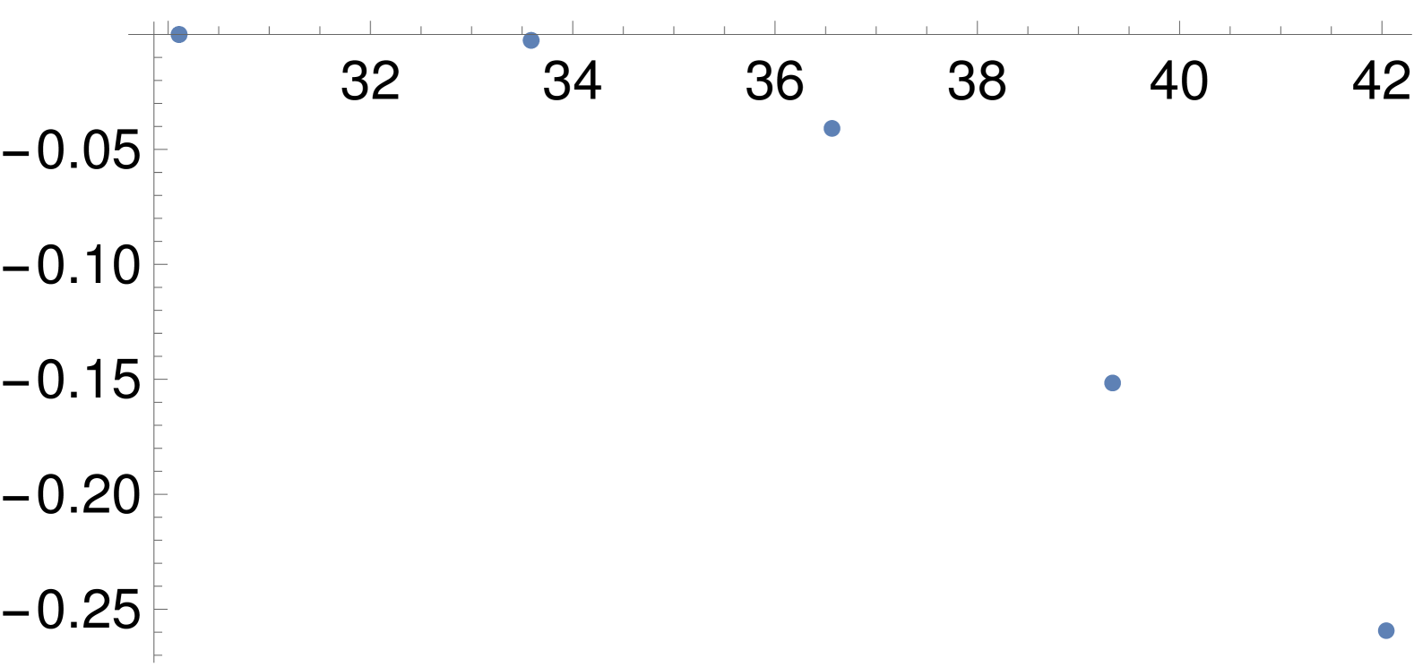
(a) Zeros obtained using the Newton method starting from the real axis (by varying the initial guess $k_{0}$ from $0$ to $40$) for $n_{1}=1.5$ and $m=40$.

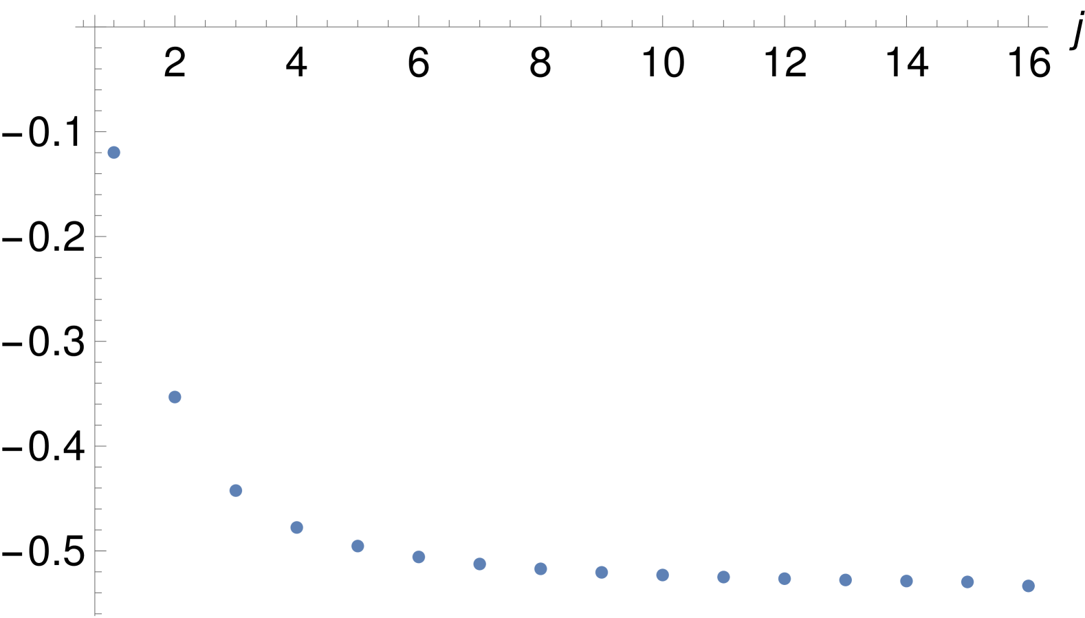
(b) Plot of $\Im(k_{m,j})$ versus $j$ for $n_{1}=1.5$ and $m=10$.

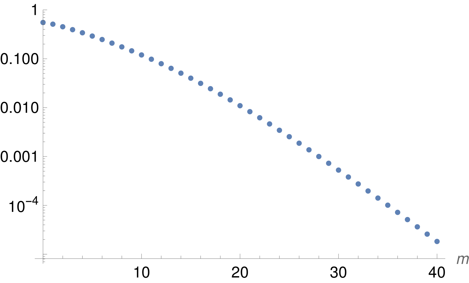
(c) Log plot of $|\Im(k_{m,1})|$ versus $m$ for $n_{1}=1.5$.

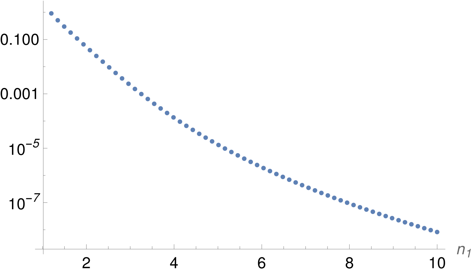
(d) Log plot of $|\Im(k_{m,1}(n_{1}))|$ versus $n_{1}$ for $m=5$.

Figure 1: Some features of resonances in the piecewise constant case for $n_{2}=1$ and $\xi=1$.

4.2.5 Choice of $h_{1,1,k}$ and $h_{2,2,k}$: proper conditioning

Note that $f_{1,1,k}$ and $f_{2,2,k}$, when uniquely defined as solutions of (23), are given by $r\mapsto J_{m}(kn_{1}r)$ and $r\mapsto H_{m}(kn_{2}r)$ respectively in the piecewise constant case, for a specific choice of $h_{1,1,k}$ and $h_{2,2,k}$ namely

$$\begin{dcases}h_{1,1,k}=kn_{1}(\xi)J^{\prime}_{m}(k\xi n_{1}(\xi))-ikn_{1}(\xi)J_{m}(k\xi n_{1}(\xi))=kn_{1}(\xi)[J^{\prime}_{m}(k\xi n_{1}(\xi))-iJ_{m}(k\xi n_{1}(\xi))]=:\frac{1}{c_{1,k}}\\ h_{2,2,k}=-kn_{2}(\xi)H^{\prime}_{m}(k\xi n_{2}(\xi))-ikn_{2}(\xi)H_{m}(k\xi n_{2}(\xi))=-kn_{2}(\xi)[H^{\prime}_{m}(k\xi n_{2}(\xi))+iH_{m}(k\xi n_{2}(\xi))]=:\frac{1}{c_{2,k}},\end{dcases}$$ (59)

Lemma 10.

For all $k\in\mathbb{C}_{\geq 0}^{\ast}$ and all $\xi\in{]}0,1[$, $J_{m}^{\prime}(k\xi n_{1}(\xi))-iJ_{m}(k\xi n_{1}(\xi))\neq 0$ and $H_{m}^{\prime}(k\xi n_{2}(\xi))+iH_{m}(k\xi n_{2}(\xi))\neq 0$.

Proof.

Let $k\in\mathbb{C}_{\geq 0}^{\ast}$. Following Lemma 4 (Examples 3.a-5.a and 3.c-5.c), the function $r\mapsto J_{m}(kn_{1}(\xi)r)$ is the unique solution of the differential equation

$$\begin{dcases}-y^{\prime\prime}(r)-\frac{1}{r}y^{\prime}(r)+\Bigl{(}\frac{m^{2}}{r^{2}}-k^{2}n_{1}^{2}(\xi)\Bigr{)}y(r)=0&\text{in $(0,\xi)$}\\ y^{\prime}(\xi)-ikn_{1}(\xi)y(\xi)=kn_{1}(\xi)J^{\prime}_{m}(k\xi n_{1}(\xi))-ikn_{1}(\xi)J_{m}(k\xi n_{1}(\xi))&\text{Robin boundary conditions}\\ y(0)=0&\text{for odd $m$}\\ y^{\prime}(0)=0&\text{for even $m$}.\end{dcases}$$ (60)

If there exists $k\in\mathbb{C}_{\geq 0}^{\ast}$ such that $J^{\prime}_{m}(k\xi n_{1}(\xi))-iJ_{m}(k\xi n_{1}(\xi))=0$ then the solution $r\mapsto J_{m}(kn_{1}(\xi)r)$ is identically zero. This is a contradiction. For the result concerning $H_{m}$, we use a similar reasoning considering the unique solution of the differential equation

$$\begin{dcases}-y^{\prime\prime}(r)-\frac{1}{r}y^{\prime}(r)+\Bigl{(}\frac{m^{2}}{r^{2}}-k^{2}n_{2}^{2}(\xi)\Bigr{)}y(r)=0&\text{in $(\xi,1)$}\\ -y^{\prime}(\xi)-ikn_{2}(\xi)y(\xi)=-kn_{2}(\xi)H^{\prime}_{m}(k\xi n_{2}(\xi))-ikn_{2}(\xi)H_{m}(k\xi n_{2}(\xi))&\text{Robin boundary conditions}\\ y^{\prime}(1)-kn_{2}(\xi)\frac{H^{\prime}_{m}(kn_{2}(\xi))}{H_{m}(kn_{2}(\xi))}y(1)=0&\text{DtN boundary conditions}\end{dcases}$$ (61)

since $H_{m}(kn_{2}(\xi))\neq 0$ for $k\in\mathbb{C}_{\geq 0}^{\ast}$ (for integer orders $m$, the zeros of the Hankel function of the first kind always have negative imaginary parts [1]). ∎

Lemma 11.

Let Assumption 6 be satisfied in the piecewise constant case, for a resonance $(\tilde{k},\tilde{u})\in{\mathbb{C}}_{<0}\times H^{1}(\Omega)\setminus\{0\}$ of problem 4 and neighborhood $\omega_{\tilde{k}}$ as in Assumption 6. Then, for any $k\in\omega_{\tilde{k}}$, $J_{m}^{\prime}(k\xi n_{1}(\xi))-iJ_{m}(k\xi n_{1}(\xi))\neq 0$ and $H_{m}^{\prime}(k\xi n_{2}(\xi))+iH_{m}(k\xi n_{2}(\xi))\neq 0$.

Proof.

Under Assumption 6, problems (23) are well posed for all $k\in\omega_{\tilde{k}}$. Using the same reasoning as in the proof of Lemma 10, it follows that for any $k\in\omega_{\tilde{k}}$, $J_{m}^{\prime}(k\xi n_{1}(\xi))-iJ_{m}(k\xi n_{1}(\xi))\neq 0$ and $H_{m}^{\prime}(k\xi n_{2}(\xi))+iH_{m}(k\xi n_{2}(\xi))\neq 0$, since the contrary leads to a contradiction. ∎

Remark 3.

It follows that, in the piecewise constant case, the resonances of the auxiliary problems in (23) are respectively the zeros of $\frac{1}{c_{1k}}$ and the zeros of $\frac{1}{c_{2k}}$ (59).

For the simplest choice $h_{1,1,k}=h_{2,2,k}=1$, it holds

$$\begin{dcases}f_{1,1,k}(r)=c_{1,k}J_{m}(kn_{1}r)\\ f_{2,2,k}(r)=c_{2,k}H_{m}(kn_{2}r),\end{dcases}$$ (62)

when the fundamental system (23) is well posed, and the Newton algorithm on this choice (leading to “$\mathrm{det}_{2}$”) could have a different behavior than the one (“$\mathrm{det}_{1}$”) in (51) as, even if

$$\mathrm{det}_{2}(k)=c_{1,k}c_{2,k}\mathrm{det}_{1}(k)=\alpha(k)\mathrm{det}_{1}(k)$$ (63)

for some function $\alpha$ satisfying $\alpha(k)\neq 0$ for all $k\in\omega_{\tilde{k}}$ (Lemma 11), one has

$$\frac{\mathrm{det}_{2}(k)}{\partial_{k}\mathrm{det}_{2}(k)} =\frac{c_{1,k}c_{2,k}\mathrm{det}_{1}(k)}{\partial_{k}c_{1,k}c_{2,k}\mathrm{det}_{1}(k)+c_{1,k}\partial_{k}c_{2,k}\mathrm{det}_{1}(k)+c_{1,k}c_{2,k}\partial_{k}\mathrm{det}_{1}(k)}$$ (64)

$$=\frac{1}{\frac{\partial_{k}c_{1,k}}{c_{1,k}}+\frac{\partial_{k}c_{2,k}}{c_{2,k}}+\frac{\partial_{k}\mathrm{det}_{1}(k)}{\mathrm{det}_{1}(k)}}$$ (65)

$$\neq\frac{\mathrm{det}_{1}(k)}{\partial_{k}\mathrm{det}_{1}(k)}.$$ (66)

Indeed, in our experiments, the use of $\mathrm{det_{2}}$ may cause some roundoff problems as the ratio $\frac{\partial_{k}\mathrm{det}_{2}(k)}{\mathrm{det}_{2}(k)}$ may be close to zero in contrast to $\frac{\partial_{k}\mathrm{det}_{1}(k)}{\mathrm{det}_{1}(k)}$, see Figure 2.

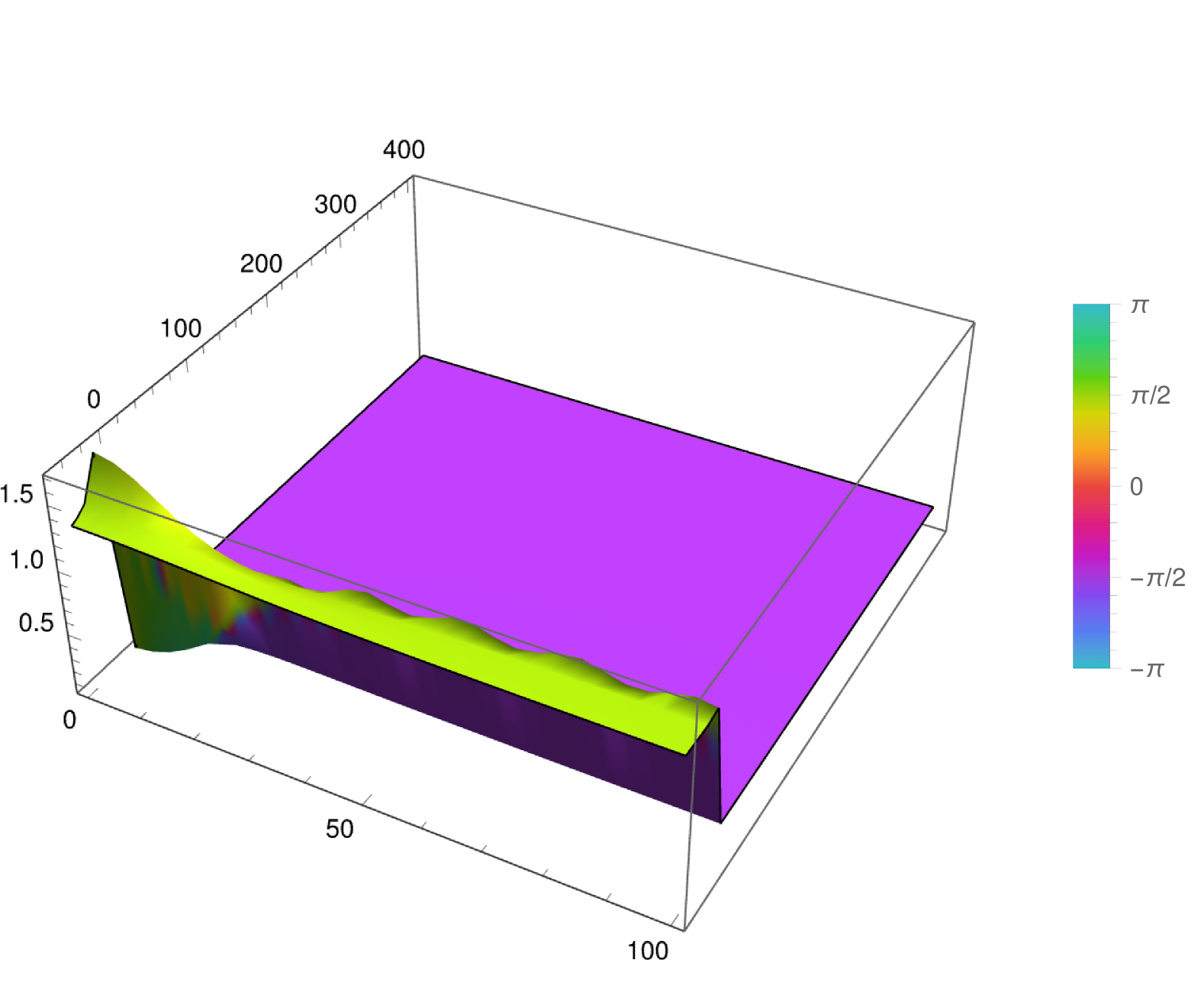
(a) $\frac{\partial_{k}\mathrm{det}_{1}(k)}{\mathrm{det}_{1}(k)}$

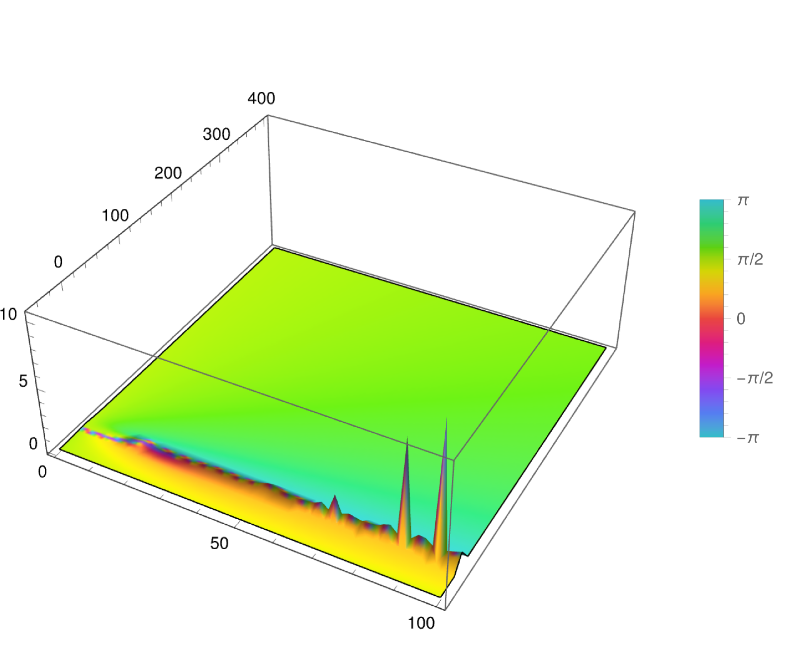
(b) $\frac{\partial_{k}\mathrm{det}_{2}(k)}{\mathrm{det}_{2}(k)}$

Figure 2: Comparison between $\frac{\partial_{k}\mathrm{det}_{2}(k)}{\mathrm{det}_{2}(k)}$ and $\frac{\partial_{k}\mathrm{det}_{1}(k)}{\mathrm{det}_{1}(k)}$ for $\xi=0.5$, $n_{1}=1.5$, $n_{2}=1$ and $m=10$. Here $k$ is varying over the complex rectangle with vertices $-50i$ and $100+400i$.

Another observation regarding the use of the Newton method with $\mathrm{det}_{2}$ starting from the real axis is that, often, the first iterate has in our experiments a positive imaginary part which is not optimal knowing that the roots satisfy $\Im(k)<0$. This is related to the sign of $\Im\bigl{(}\frac{\det(k_{0})}{\partial_{k}\mathrm{det}(k_{0})}\bigr{)}$: if it is positive then the first iterate has a negative imaginary part, otherwise it has a positive imaginary part. We plot this quantity $\Im\bigl{(}\frac{\det(k_{0})}{\partial_{k}\mathrm{det}(k_{0})}\bigr{)}$ for $k_{0}\in{\mathbb{R}}_{>0}$ in Figure 3 for different choices of determinants: $\mathrm{det}_{1}$ or $\mathrm{det}_{2}$, we also considered $\mathrm{det}_{\mathrm{scal}}$ corresponding to the scaling

$$\mathrm{det}_{\mathrm{scal}}(k)=k^{2}\mathrm{det}_{2}(k)$$ (67)

in order to investigate whether a simpler scaling than multiplying $\mathrm{det}_{2}$ by $\frac{1}{c_{1,k}c_{2,k}}$ would be suitable in practice. In Appendix B, we gathered complex plots of the different scalings of the determinant.

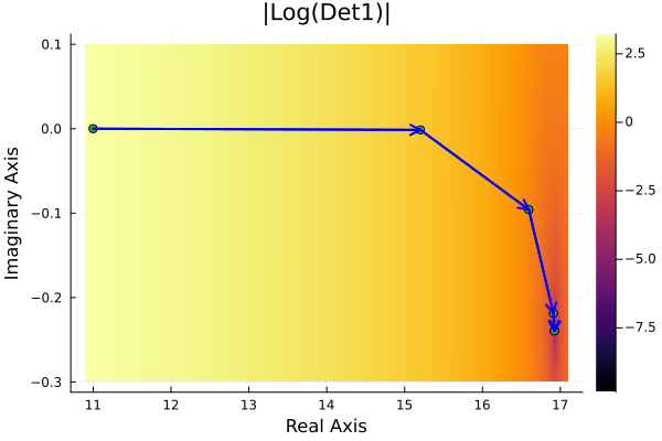
(a)

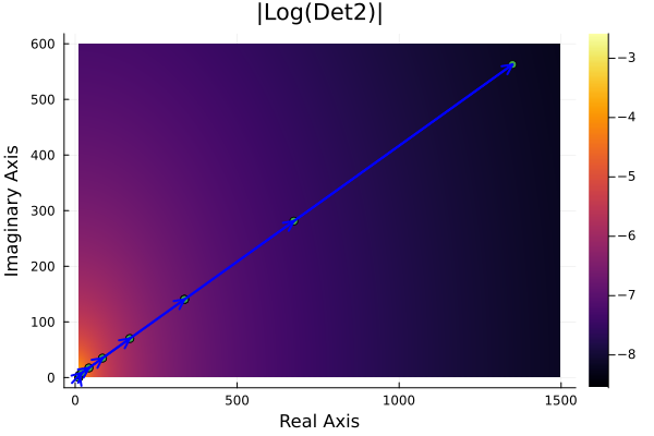
(b)

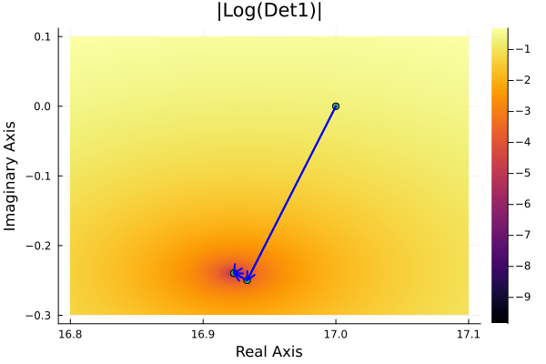
(c)

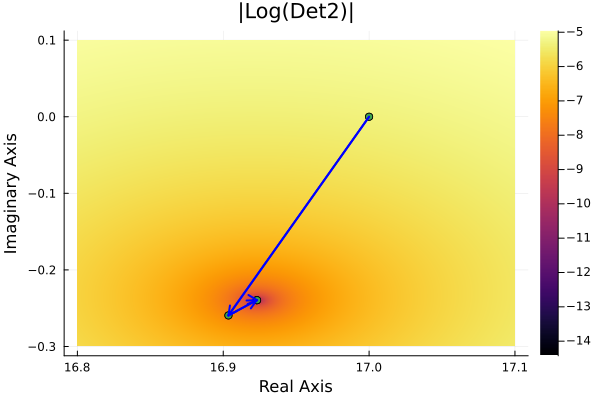
(d)

Figure 10: Newton iterations in the complex plane using $\det_{1}$ or $\det_{2}$ for $\xi=0.5$, $n_{1}=1.5$, $n_{2}=1$ and $m=10$, starting from $k_{0}=11$ (top) or $k_{0}=17$ (bottom).

As shown in Figure 3, the considered quantity is always positive for $\mathrm{det}_{1}$ in contrast to $\mathrm{det}_{2}$ which has an oscillatory behavior. It appears that the simpler scaling by $k^{2}$ does not resolve the problem of negative imaginary parts on the real axis, and it seems that a scaling that is oscillatory with $k$ is advantageous. For certain values of $k_{0}$, however, the quantity $\frac{\det_{2}(k_{0})}{\partial_{k}\mathrm{det}_{2}(k_{0})}$ is positive, and the Newton algorithm should work better for these initial starting points (tests performed for $k_{0}=17$ or $k_{0}=22$ for $\xi=0.5$, $n_{1}=1.5$, $n_{2}=1$ and $m=10$). Figure 10 and Table 3 show the Newton iterations in the complex plane for two choices of the initial guess on the real axis, where one can witness either a convergence or a gross divergence using $\det_{2}$. In Appendix B, we explore the reasons behind this behavior in more depth. Given that we intend to propose a Newton technique that starts on the real axis, we recommend to start the algorithm with a first iteration in the fourth quadrant, so that $\Im(k_{1})<0$.

In the variable case, the insights gained from the piecewise constant case will be useful to ensure that the problem is scaled properly, see Assumption 14.

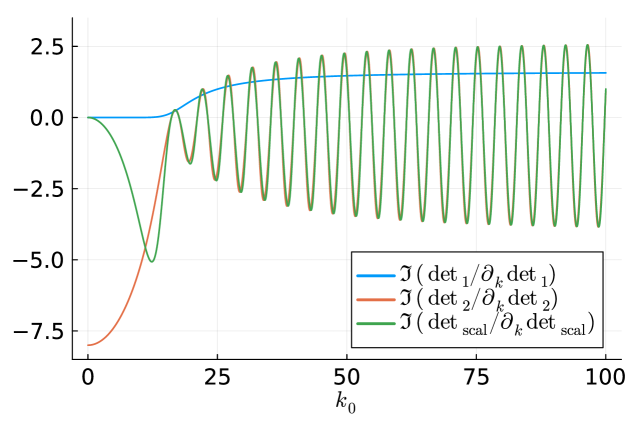
Figure 3: Plot of $\Im\bigl{(}\frac{\det(k_{0})}{\partial_{k}\mathrm{det}(k_{0})}\bigr{)}$ on the real axis for $\xi=0.5$, $n_{1}=1.5$, $n_{2}=1$ and $m=10$.

5 Variable case

In the variable case, one needs to solve the boundary value problems numerically to compute $f_{1,1,k}$, $f_{2,2,k}$, $\partial_{k}f_{1,1,k}$ and $\partial_{k}f_{2,2,k}$ necessary for the expression of the determinant and to the Newton algorithm implementation. Hence, there is a need for reliable BVP solver of these ODEs.

Since the problems posed in $(0,\xi)$ and $(\xi,1)$ are Bessel-type equations, their numerical approximation can be challenging given the singularities in the equation and the oscillatory behavior of the solution. To circumvent these problems, we use spectral methods in order to achieve high accuracy approximation. This is based on the asymptotic expansion of the solution on a given basis and we adopt the ApproxFun package in Julia language [46]. This is more efficient and reliable than using NDSolve of Mathematica and it is more suitable for numerical computations.

5.1 Convergence of the Newton method: simplicity of the roots (see definition in Appendix C)

5.1.1 Geometric simplicity

Proposition 12.

Let $\lambda\in{\mathbb{C}}^{*}$ be an eigenvalue of the nonlinear eigenvalue problem (24) (under Assumption 6). Then $\lambda$ is geometrically simple.

Proof.

Let $\begin{pmatrix}x_{1}\\ x_{2}\end{pmatrix}\in{\mathbb{C}}^{2}\setminus\{0\}$ be an eigenvector corresponding to the eigenvalue $\lambda$, i.e.,

$$f^{\prime}_{1,1,\lambda}(\xi)f_{2,2,\lambda}(\xi)-f_{1,1,\lambda}(\xi)f^{\prime}_{2,2,\lambda}(\xi)=0$$ (68)

and

$$\begin{dcases}f_{1,1,\lambda}(\xi)x_{1}-f_{2,2,\lambda}(\xi)x_{2}=0\\ f^{\prime}_{1,1,\lambda}(\xi)x_{1}-f^{\prime}_{2,2,\lambda}(\xi)x_{2}=0.\end{dcases}$$ (69)

From $f^{\prime}_{1,1,\lambda}(\xi)-i\lambda n_{1}(\xi)f_{1,1,\lambda}(\xi)=h_{1,1,\lambda}\neq 0$ (8) (resp. $-f^{\prime}_{2,2,\lambda}(\xi)-i\lambda n_{2}(\xi)f_{2,2,\lambda}(\xi)=h_{2,2,\lambda}\neq 0$ (10)), we get that $f_{1,1,\lambda}(\xi)$ and $f^{\prime}_{1,1,\lambda}(\xi)$ cannot vanish simultaneously (resp. $f_{2,2,\lambda}(\xi)$ and $f^{\prime}_{2,2,\lambda}(\xi)$ cannot vanish simultaneously). Moreover, from (68), $f_{1,1,\lambda}(\xi)=0$ if and only if $f_{2,2,\lambda}(\xi)=0$ (resp. $f^{\prime}_{1,1,\lambda}(\xi)=0$ if and only if $f^{\prime}_{2,2,\lambda}(\xi)=0$). By using this in (69) we conclude that, there exists a nonzero complex constant $C_{\lambda}\in\Bigl{\{}\frac{f_{2,2,\lambda}(\xi)}{f_{1,1,\lambda}(\xi)},\frac{f^{\prime}_{2,2,\lambda}(\xi)}{f^{\prime}_{1,1,\lambda}(\xi)}\Bigr{\}}$ such that

$$x_{1}=C_{\lambda}x_{2},$$ (70)

and any eigenvector corresponding to the same eigenvalue $\lambda$ can be written $x_{2}\begin{pmatrix}C_{\lambda}\\ 1\end{pmatrix}$ hence ${\dim(\ker(T(\lambda)))=1}$, i.e., the eigenvalue $\lambda$ is geometrically simple. ∎

Remark 4.

One could also adapt the proof of the simplicity of eigenvalues for Sturm-Liouville problems [13, Thm. 11.2.3] [51, Thm. 2.4] to our case, and show the simplicity of eigenvalues for the ODE (7) with $\hat{g}_{m}=0$ and then deduce the geometric simplicity of the eigenvalues for the corresponding nonlinear eigenvalue problem.

5.1.2 Algebraic simplicity

Proposition 13.

Let $\lambda\in{\mathbb{C}}^{*}$ be an eigenvalue of the nonlinear eigenvalue problem (24) (under Assumption 6). Then $\lambda$ is not algebraically simple if and only if

$$\begin{array}[]{c@{\quad}|c}\text{(Case $f^{(0)}_{1,1,\lambda}(\xi)\neq 0$)}&\text{(Case $f^{(0)}_{1,1,\lambda}(\xi)=0$)}\\[5.0pt] \begin{dcases}f^{(0)}_{1,1,\lambda}(\xi)\neq-1\\ f^{(0)}_{2,2,\lambda}(\xi)=-\frac{f^{(0)}_{1,1,\lambda}(\xi)}{f^{(0)}_{1,1,\lambda}(\xi)+1}\\ \partial_{k}f^{0}_{1,1,k}(\xi)_{|k=\lambda}=-\frac{f^{0}_{1,1,\lambda}(\xi)(f^{0}_{1,1,\lambda}(\xi)+1)}{\lambda}\\ \partial_{k}f^{(0)}_{2,2,k}(\xi)_{|k=\lambda}=-\frac{f^{(0)}_{2,2,\lambda}(\xi)}{\lambda},\end{dcases}&\begin{dcases}f^{(0)}_{1,1,\lambda}(\xi)=0\\ f^{(0)}_{2,2,\lambda}(\xi)=0\\ \partial_{k}f^{(0)}_{2,2,k}(\xi)_{|k=\lambda}=-\partial_{k}f^{(0)}_{1,1,k}(\xi)_{|k=\lambda},\end{dcases}\end{array}$$ (71)

where $f^{(0)}_{i,i,\lambda}(r)=\frac{f_{i,i,\lambda}(r)}{l_{i,i,\lambda}}$ for $i\in\{1,2\}$ (notations as in Remark 2). Note that the first two lines simply reflect the fact that $\lambda$ is an eigenvalue ($D^{(0)}(\lambda)=0$).

Proof.

Using notations of Remark 2, we assume, without loss of generality, $l^{(0)}_{1,1,k}=l^{(0)}_{2,2,k}=1$. Indeed, for general choices of $l_{1,1,k}\neq 0$ and $l_{2,2,k}\neq 0$ for $k\neq 0$, we deduce, using (42), that $\lambda\in{\mathbb{C}}^{*}$ is not an algebraic simple eigenvalue if and only if

$$\begin{dcases}\det(\lambda)=0\\ \partial_{k}\det(\lambda)=0\end{dcases} \iff\begin{dcases}{\det}^{(0)}(\lambda)=0\\ \partial_{k}[l_{1,1,k}l_{2,2,k}]_{|k=\lambda}{\det}^{(0)}(\lambda)+l_{1,1,\lambda}l_{2,2,\lambda}\partial_{k}{\det}^{(0)}(\lambda)=0\end{dcases}$$ (72)

$$\iff\begin{dcases}{\det}^{(0)}(\lambda)=0\\ \partial_{k}{\det}^{(0)}(\lambda)=0\end{dcases}\iff\begin{dcases}D^{(0)}(\lambda)=0\\ \partial_{k}D^{(0)}(\lambda)=0,\end{dcases}$$ (73)

i.e. if and only if $\lambda$ is not an algebraic simple eigenvalue of the nonlinear eigenvalue problem $T^{(0)}(k)A=0$ (24) with the specific choices $f^{(0)}_{1,1,k}$ and $f^{(0)}_{2,2,k}$. Moreover, since $\lambda$ is geometrically simple (Proposition 12), $\lambda$ is not algebraically simple if and only if $y^{*}[\partial_{k}T^{(0)}(\lambda)]x=0$ where $(y,\lambda,x)$ is an eigentriplet of $T^{(0)}$.

To simplify the exposition, we will use in this proof the following notations:

$$F_{1} =f^{(0)}_{1,1,k}(\xi) F_{2} =f^{(0)}_{1,1,k}(\xi) F_{1}^{\prime} =(f^{(0)}_{1,1,k})^{\prime}(\xi) F_{2}^{\prime} =(f^{(0)}_{2,2,k})^{\prime}(\xi)$$ (74)

$$\partial_{k}F_{1} =\partial_{k}f^{(0)}_{1,1,k}(\xi) \partial_{k}F_{2} =\partial_{k}f^{(0)}_{2,2,k}(\xi) N_{1} =n_{1}(\xi) N_{2} =n_{2}(\xi).$$ (75)

Let $y=\begin{pmatrix}y_{1}\\ y_{2}\end{pmatrix}\in{\mathbb{C}}^{2}\setminus\{0\}$ be a left eigenvector for the eigenvalue $\lambda$ (i.e. $T^{(0)}(\lambda)^{*}y=0$). Then, at $k=\lambda$,

$$\begin{dcases}F^{\prime}_{1}F_{2}-F_{1}F^{\prime}_{2}=0\\ \overline{F_{1}}y_{1}+\overline{F^{\prime}_{1}}y_{2}=0\\ -\overline{F_{2}}y_{1}-\overline{F_{2}^{\prime}}y_{2}=0.\end{dcases}$$ (76)

From the proof of the geometric simplicity, we have, at $k=\lambda$,

$$F_{i} F_{i}^{\prime} F_{1}=0\iff F_{2}=0, F^{\prime}_{1}=0\iff F^{\prime}_{2}=0.$$ and cannot vanish simultaneously, (77)

Thus

$$y=\begin{pmatrix}-\overline{F^{\prime}_{1}}\\ \overline{F_{1}}\end{pmatrix}\propto\begin{pmatrix}-\overline{F^{\prime}_{2}}\\ \overline{F_{2}}\end{pmatrix}\neq 0$$ (78)

is a solution and (up to a multiplicative constant)

$$y^{*}=\begin{pmatrix}-F^{\prime}_{1}&F_{1}\end{pmatrix}\propto\begin{pmatrix}-F^{\prime}_{2}&F_{2}\end{pmatrix}.$$ (79)

From the proof of the geometric simplicity, the right eigenvector is given by (up to a multiplicative constant)

$$x=\begin{pmatrix}F_{2}\\ F_{1}\end{pmatrix}\text{ if $F_{1}\neq 0$, or }\begin{pmatrix}F^{\prime}_{2}\\ F_{1}^{\prime}\end{pmatrix}\text{ if $F_{1}^{\prime}\neq 0$}.$$ (80)

Let us compute $y^{*}[\partial_{k}T^{(0)}(\lambda)]x$.

1. Case $F_{1}\neq 0$:

   $$y^{*}[\partial_{k}T^{(0)}(\lambda)]x =\begin{pmatrix}-F^{\prime}_{1}&F_{1}\end{pmatrix}\begin{pmatrix}\partial_{k}F_{1}&-\partial_{k}F_{2}\\ \partial_{k}F_{1}^{\prime}&-\partial_{k}F_{2}^{\prime}\end{pmatrix}\begin{pmatrix}F_{2}\\ F_{1}\end{pmatrix}$$

   $$=-F_{1}^{\prime}F_{2}\partial_{k}F_{1}+F_{1}^{\prime}F_{1}\partial_{k}F_{2}+F_{1}F_{2}\partial_{k}F_{1}^{\prime}-F_{1}^{2}\partial_{k}F_{2}^{\prime}.$$ (81)

   From the boundary conditions, we have

   $$F_{1}^{\prime} =ikN_{1}F_{1}+k(N_{1}+N_{2}) F_{2}^{\prime} =-ikN_{2}F_{2}-k(N_{1}+N_{2})$$ (82)

   $$\partial_{k}F_{1}^{\prime} =iN_{1}F_{1}+iN_{1}k\partial_{k}F_{1}+(N_{1}+N_{2}) \partial_{k}F_{2}^{\prime} =-iN_{2}F_{2}-iN_{2}k\partial_{k}F_{2}-(N_{1}+N_{2}).$$ (83)

   Thus, writing everything in terms of $F_{i}$ and $\partial_{k}F_{i}$,

   $$y^{*}[\partial_{k}T^{(0)}(\lambda)]x= -(i\lambda N_{1}F_{1}+\lambda(N_{1}+N_{2}))F_{2}\partial_{k}F_{1}+(i\lambda N_{1}F_{1}+\lambda(N_{1}+N_{2})))F_{1}\partial_{k}F_{2}$$

   $$+F_{1}F_{2}(iN_{1}F_{1}+iN_{1}\lambda\partial_{k}F_{1}+(N_{1}+N_{2}))-F_{1}^{2}(-iN_{2}F_{2}-iN_{2}\lambda\partial_{k}F_{2}-(N_{1}+N_{2})))$$

   $$= (N_{1}+N_{2})(-\lambda F_{2}\partial_{k}F_{1}+\lambda(iF_{1}^{2}+F_{1})\partial_{k}F_{2}+iF_{1}^{2}F_{2}+F_{1}F_{2}+F_{1}^{2}).$$ (84)

2. Case $F_{1}=0$ ($\iff F_{2}=0$):

   $$y^{*}[\partial_{k}T^{(0)}(\lambda)]x =\begin{pmatrix}-F^{\prime}_{1}&0\end{pmatrix}\begin{pmatrix}\partial_{k}F_{1}&-\partial_{k}F_{2}\\ \partial_{k}F_{1}^{\prime}&-\partial_{k}F_{2}^{\prime}\end{pmatrix}\begin{pmatrix}F^{\prime}_{2}\\ F^{\prime}_{1}\end{pmatrix}=-F_{1}^{\prime}F_{2}^{\prime}\partial_{k}F_{1}+(F_{1}^{\prime})^{2}\partial_{k}F_{2}$$

   $$=-\lambda(N_{1}+N_{2})(-\lambda(N_{1}+N_{2}))\partial_{k}F_{1}+(\lambda(N_{1}+N_{2}))^{2}\partial_{k}F_{2}$$

   $$=\lambda^{2}(N_{1}+N_{2})^{2}(\partial_{k}F_{1}+\partial_{k}F_{2}).$$ (85)

Simplifying the equations $D^{(0)}(\lambda)=\partial_{k}D^{(0)}(\lambda)=y^{*}[\partial_{k}T^{(0)}(\lambda))x=0$ yields the announced result. Indeed, denoting by $a,b,c,d$ the quantities $F_{1},F_{2},\partial_{k}F_{1},\partial_{k}F_{2}$ at $k=\lambda$, the system reads (see Remark 2)

1. Case $a\neq 0$:

$$\begin{dcases}ab+a+b=0\\ cb+ad+c+d=0\\ -\lambda bc+\lambda(ia^{2}+a)d+ia^{2}b+ab+a^{2}=0\end{dcases}\iff\begin{dcases}a\neq-1\\ b=-\frac{a}{a+1}\\ c=-\frac{d(a+1)}{b+1}=-d(a+1)^{2}\\ -\lambda\left(-\frac{a}{a+1}\right)(-d(a+1)^{2})+\lambda(ia^{2}+a)d+(ia^{2}+a)\frac{-a}{a+1}+a^{2}=0\end{dcases}$$

$$\iff\begin{dcases}a\neq-1\\ b=-\frac{a}{a+1}\\ c=-\frac{d(a+1)}{b+1}=-d(a+1)^{2}\\ \lambda da(-a-1+ia+1)+a^{2}\frac{a+1-ia-1}{a+1}=0\end{dcases}\iff\begin{dcases}a\neq-1\\ b=-\frac{a}{a+1}\\ c=-d(a+1)^{2}=-\frac{a(a+1)}{\lambda}\\ d=\frac{a}{\lambda(a+1)}=-\frac{b}{\lambda}.\end{dcases}$$ (86)

1. Case $a=0$ ($\iff b=0$):

   $$\begin{dcases}ab+a+b=0\\ cb+ad+c+d=0\\ c+d=0\end{dcases}\iff\begin{dcases}a=b=0\\ d=-c.\end{dcases}$$ (87)

∎

Remark 5.

We can recover general conditions for $l_{1,1,k}\neq 0$ and $l_{2,2,k}\neq 0$ for $k\neq 0$ using (41). We obtain the following necessary and sufficient condition for an eigenvalue not to be algebraically simple:

$$\begin{array}[]{c@{\quad}|c}\text{(Case $f_{1,1,\lambda}(\xi)\neq 0$)}&\text{(Case $f_{1,1,\lambda}(\xi)=0$)}\\[5.0pt] \begin{dcases}f_{1,1,\lambda}(\xi)\neq-l_{1,1,\lambda}\\ f_{2,2,\lambda}(\xi)=-l_{2,2,\lambda}\frac{f_{1,1,\lambda}(\xi)}{f_{1,1,\lambda}(\xi)+l_{1,1,\lambda}}\\ \partial_{k}f_{1,1,k}(\xi)_{|k=\lambda}=\frac{{\partial_{k}l_{1,1,k}}_{|k=\lambda}}{l_{1,1,\lambda}}f_{1,1,\lambda}(\xi)-\frac{1}{l_{1,1,\lambda}}\frac{f_{1,1,\lambda}(\xi)(f_{1,1,\lambda}(\xi)+l_{1,1,\lambda})}{\lambda}\\ \partial_{k}f_{2,2,k}(\xi)_{|k=\lambda}=\frac{{\partial_{k}l_{2,2,k}}_{|k=\lambda}}{l_{2,2,\lambda}}f_{2,2,\lambda}(\xi)-\frac{f_{2,2,\lambda}(\xi)}{\lambda},\end{dcases}&\begin{dcases}f_{1,1,\lambda}(\xi)=0\\ f_{2,2,\lambda}(\xi)=0\\ \partial_{k}f_{2,2,k}(\xi)_{|k=\lambda}=-\frac{l_{2,2,\lambda}}{l_{1,1,\lambda}}\partial_{k}f_{1,1,k}(\xi)_{|k=\lambda}.\end{dcases}\end{array}$$ (88)

5.2 Experiments

5.2.1 Using ApproxFun to solve Bessel-type equations

Here we test the use of ApproxFun [45, 47, 57, 46] to solve the Bessel-type equations satisfied by $f_{1,1,k}$, $f_{2,2,k}$, $\partial_{k}f_{1,1,k}$ and $\partial_{k}f_{2,2,k}$. We thus test it in the piecewise constant case for which we have explicit solutions and compare the numerical solutions with the exact ones. Figure 4 shows for instance the results obtained for $\xi=0.5$, $n_{1}(r)=2$, $n_{2}(r)=1$, $m=40$ and $k=100$. Here, we took $h_{1,1,k}=h_{2,2,k}=1$.

For our purpose, we also compare in Table 2 the numerical and exact values of $\mathrm{det}(k)$ (3) and $\partial_{k}\mathrm{det}(k)$ (3) as these are the important quantities in the Newton algorithm. Note that these only depend on the values of the previous functions at the interface $\xi$.

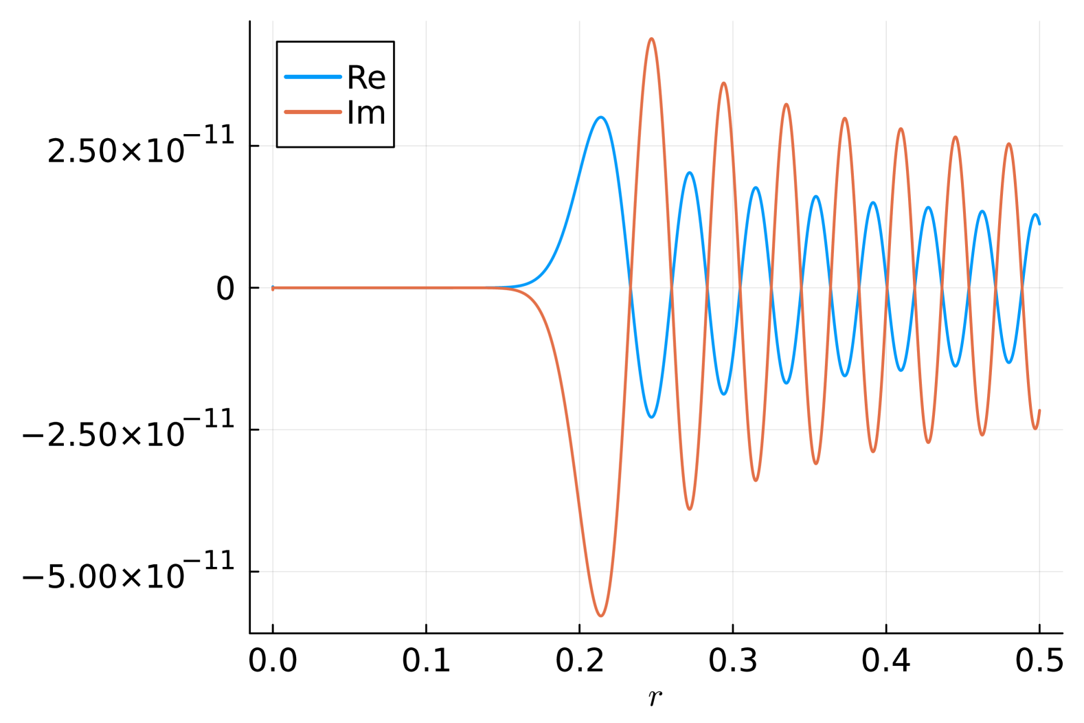
(a) $f^{\mathrm{num}}_{1,1,k}-f^{\mathrm{ex}}_{1,1,k}$

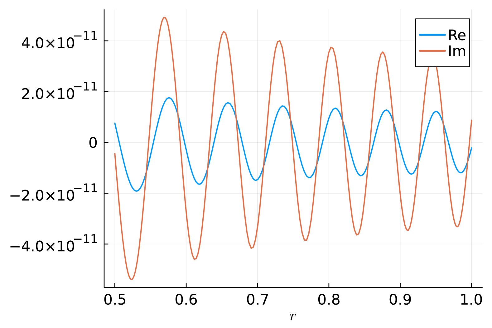
(b) $f^{\mathrm{num}}_{2,2,k}-f^{\mathrm{ex}}_{2,2,k}$

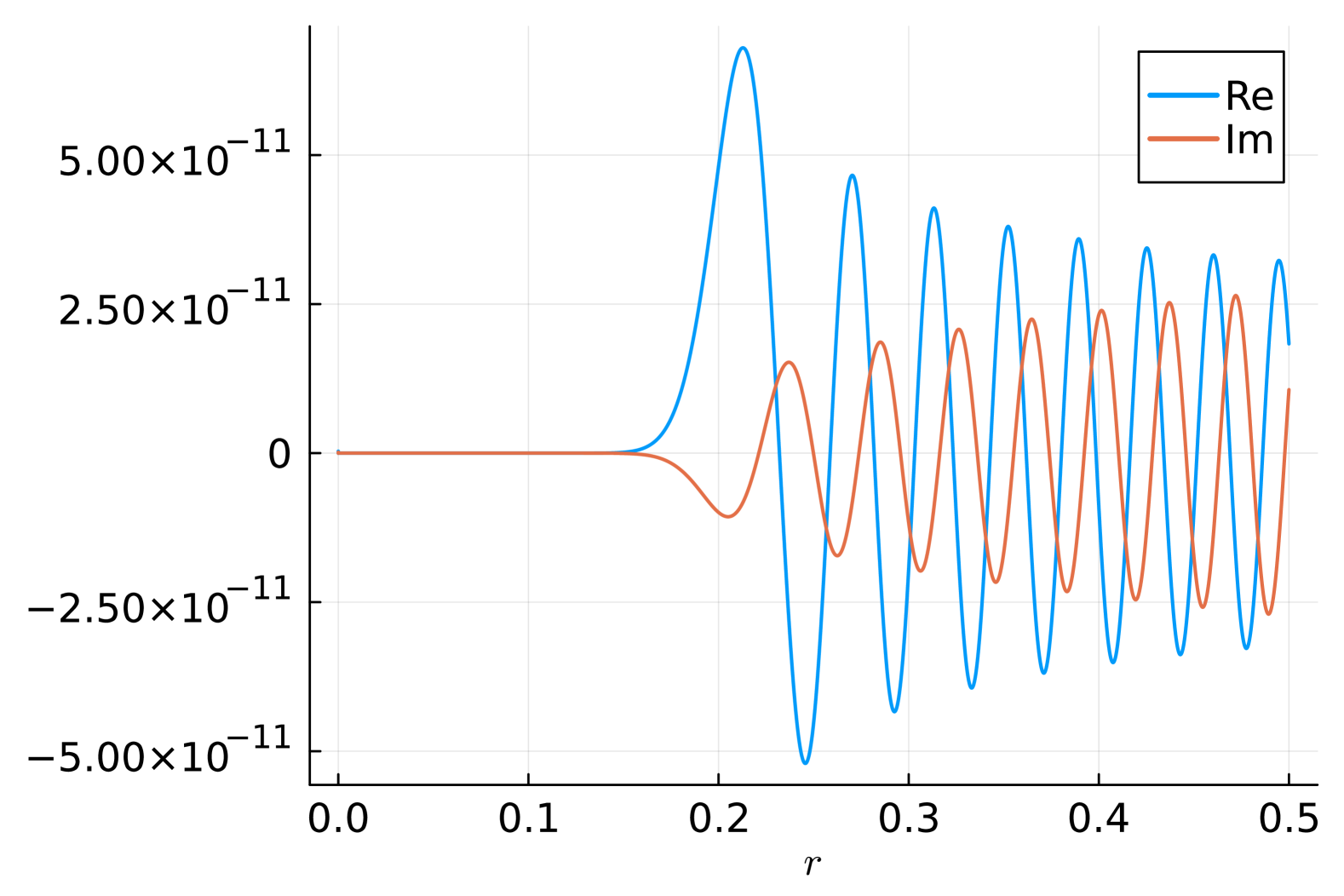
(c) $\partial_{k}f^{\mathrm{num}}_{1,1,k}-\partial_{k}f^{\mathrm{ex}}_{1,1,k}$

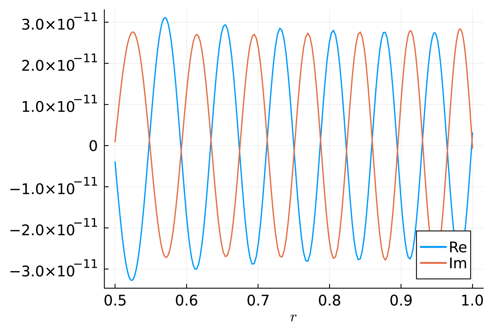
(d) $\partial_{k}f^{\mathrm{num}}_{2,2,k}-\partial_{k}f^{\mathrm{ex}}_{2,2,k}$

Figure 4: Errors between numerical solutions using ApproxFun and exact solutions for $\xi=0.5$, $n_{1}(r)=2$, $n_{2}(r)=1$, $m=40$ and $k=100$.

	$\mathrm{det}(k)$	$\partial_{k}\mathrm{det}(k)$
Exact	$0.0017645943961392297+0.002741759560912059i$	$0.002252125059322991+0.0030074474911066787i$
Numerical	$0.0017645943961392056+0.002741759560912057i$	$0.00225212505932299+0.003007447491106633i$
Error	$2.413171981847463e-17$	$4.555507377576837e-17$

Table 2: Error between numerical and exact values of $\mathrm{det}(k)$ and $\partial_{k}\mathrm{det}(k)$ for $\xi=0.5$, $n_{1}(r)=2$, $n_{2}(r)=1$, $m=40$ and $k=100$.

5.2.2 Newton method using ApproxFun

We implement the Newton method in the non-constant case following the algorithm presented in Section 3.1, where we now use ApproxFun to solve numerically the different boundary value problems involved. As explained in Section 4.2.5, the choice of $h_{1,1,k}$ and $h_{2,2,k}$ seems to be important. We recall that $c_{1,k}$ and $c_{2,k}$ are defined in (59) and we will thus take the constants $h_{1,1,k}=\frac{1}{c_{1,k}}$ and $h_{2,2,k}=\frac{1}{c_{2,k}}$ leading to $f_{1,1,k}(r)=J_{m}(kn_{1}r)$ and $f_{2,2,k}(r)=H_{m}(kn_{2}r)$ in the piecewise constant case. Equivalently, and in order to compare the results with those obtained for the determinant used in the piecewise constant case (which was actually $D(k)=\frac{\mathrm{det}_{1}(k)}{k}~\eqref{eq:determinantpwconstant}$), we choose $h_{1,1,k}=h_{2,2,k}=1$ leading to “$\mathrm{det}_{2}$” and then proceed with the following scaling for the determinant:

$$D(k)=\frac{1}{kc_{1,k}c_{2,k}}{\mathrm{det}_{2}(k)}$$ (89)

whose derivative is obtained knowing $\mathrm{det}_{2}(k)$ and $\partial_{k}\mathrm{det}_{2}(k)$ by

$$\partial_{k}D(k)=\frac{1}{kc_{1,k}c_{2,k}}{\partial_{k}\mathrm{det}_{2}(k)}+\partial_{k}\Big{(}\frac{1}{kc_{1,k}c_{2,k}}\Bigr{)}{\mathrm{det}_{2}(k)}.$$ (90)

For this purpose, we will need an additional assumption in the variable case:

Assumption 14.

Let $\left(\tilde{k},\tilde{u}\right)\in\mathbb{C}_{<0}\times H_{0}^{1}\left(\Omega\right)\setminus\{0\}$ be a resonance of problem (4) and $m\in\mathbb{Z}$. Then, there exists a complex neighborhood $\omega_{\tilde{k}}\subset\mathbb{C}_{<0}$ of $\tilde{k}$ such that $\frac{1}{c_{1,k}}\neq 0$ and $\frac{1}{c_{2,k}}\neq 0$ for all $k\in\omega_{\tilde{k}}$.

In this way, it is assumed that the resonances of the non-linear eigenvalue problem (4) are not simultaneously zeros of $\frac{1}{c_{1k}}$ or $\frac{1}{c_{2k}}$ .

5.2.2.1 Constant case validation

We perform here the Newton method using ApproxFun package (in Julia) in the piecewise constant case and compare it to the Newton method performed using the exact expression (51) of $D(k)$ (in Mathematica). Tables S-1 and S-2 summarize the results obtained for $\xi=0.5$, $m=10$, $n_{1}=1.5$ and $n_{2}=1$. We took $\varepsilon=10^{-6}$ and $l_{\max}=1000$. The results are mostly the same: there is convergence of the Newton method with the same number of iterations except for $k_{0}=19$ that does not converge in the specified number of iterations. Increasing $l_{\max}$ to $10000$ yields the same result.

5.2.2.2 Variable cases validation

5.2.2.2.1 A perturbation of a constant by a bump function

We consider here a non-constant refractive index, where $n_{1}$ is a perturbation of a constant by some bump function. More concretely, we choose $\xi=0.5$,

$$n_{1}(r)=1.5+\exp\Bigl{(}-\frac{1}{1-(4r-1)^{2}}\Bigr{)}$$ (91)

and keep $n_{2}(r)=1$ constant. The results are shown in Table S-3 for $\xi=0.5$ and $m=10$. In this case, we obtain asymptotically for large $m$ the same results as for the constant case $n_{1}=1.5$ (Tables S-1 and S-2). This is consistent with results in [10] (Appendix D) since this choice of $n_{1}(r)$ satisfies $n_{1}(\xi)=1.5$ and $n_{1}^{\prime}(\xi)=n_{1}^{\prime\prime}(\xi)=0$ thus the quantities $\check{\kappa}=1$ and $\check{\mu}=2$ in [10] result in the same asymptotic expansions for resonances as for the constant case $n_{1}=1.5$ .

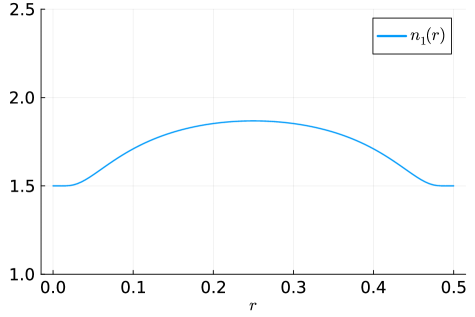
Figure 5: Plot of $n_{1}(r)$ (91).

5.2.2.2.2 A special variable case with explicit solution

We consider here the special choice of $n_{1}$:

$$n_{1}(r)=\sqrt{2-r^{2}}$$ (92)

for which the solution of (8) on $(0,\xi)$ is (up to within a multiplicative constant)

$$f_{0}(x)=\frac{1}{x}M_{\frac{k}{2},\frac{m}{2}}(kx^{2})$$ (93)

where $M_{k,m}(z)$ is the Whittaker function (see Appendix E).

If we consider a constant $n_{2}=1$, then the fundamental solutions $f_{1,1,k}$ and $f_{2,2,k}$ are explicitly given by:

$$f_{1,1,k}(r) =\frac{\frac{1}{c_{1,k}}}{f_{0}^{\prime}(\xi)-ikn_{1}(\xi)f_{0}(\xi)}f_{0}(r)$$

$$f_{2,2,k}(r) =H_{m}(kn_{2}r);$$

using our scaling. This allows us to construct the exact determinant using formula (25) and we then work with the corresponding $D(k)=\frac{\det(k)}{k}$. We compare the results obtained using the Newton method with ApproxFun and using the exact expression of the determinant in Tables S-4 and S-5. Again, the results are very close, which validates once again our methodology and algorithm’s implementation.

5.3 Newton method for variable refractive index

Based on the previous experiments, we are going to present here the full Newton algorithm to find quasi-resonances in the variable case. We will specify in particular the choice of boundary conditions and starting values. The Newton algorithm we suggest is the following (see also Section 5.2.2 for an equivalent construction of $D(k)$) 

Algorithm 2 Newton’s algorithm for variable refractive index

 $\mathrm{Newton}\_\mathrm{var}(\xi,n_{1}(r)\text{ on }(0,\xi),n_{2}(r)\text{ on }(\xi,1),m\in{\mathbb{N}},\varepsilon,l_{\max})$

 $\bullet$ Take the starting value: $k_{0}=\frac{m}{\xi n_{1}(\xi)};$

 for $l=0\ldots$ until stopping criterion is reached do

  $\bullet$ Start with $k=k_{l};$

  $\bullet$ Solve two two-point boundary value problems numerically for $k=k_{l}$: result: approximations $f_{1,1,k}$ and $f_{2,2,k}$ to (8) and (10) with the boundary conditions

$$\begin{dcases}h_{1,1,k}=kn_{1}(\xi)(J^{\prime}_{m}(k\xi n_{1}(\xi))-iJ_{m}(k\xi n_{1}(\xi)))\quad\text{(assumed to be $\neq 0$)}\\ h_{2,2,k}=-kn_{2}(\xi)(H^{\prime}_{m}(k\xi n_{2}(\xi))+iH_{m}(k\xi n_{2}(\xi)))\quad\text{(assumed to be $\neq 0$)};\end{dcases}$$ (94)

  $\bullet$ Compute numerically the derivatives with respect to $k$, $\partial_{k}f_{1,1,k}$ and $\partial_{k}f_{2,2,k}$, as the solution of two two-point boundary value problems (43), (44);

  $\bullet$ Compute $\mathrm{det}(k_{l})$ by using (3) and $\partial_{k}\mathrm{det}(k_{l})$ by (3);

  $\bullet$ Consider the following determinant

$$D(k)=\frac{1}{k}\det(k)$$ (95)

and

$$\partial_{k}D(k)=\frac{1}{k}\partial_{k}\det(k)-\frac{1}{k^{2}}\det(k);$$ (96)

  $\bullet$ Compute

$$k_{l+1}=k_{l}-\frac{D(k_{l})}{\partial_{k}D(k_{l})};$$ (97)

  $\bullet$ $l\leftarrow l+1;$

  The stopping criterion is given by $|D(k)|\leq\varepsilon$ or when a maximal number of iterations $l_{\max}$ is reached.

 end for

5.3.1 Piecewise constant cases

We consider the following examples, where $n_{2}(r)=1$,

• $n_{1}(r)=1.5$ (Table S-6)

• $n_{1}(r)=5$ (Table S-7)

We also report on the tables the value $k_{\mathrm{asympt}}$ corresponding to the first terms of the asymptotics of $\underline{k}_{0}(m)$ up to $O(m^{-1})$ (Thm. 1.A in Appendix D).

5.3.2 Non-constant cases (illustrated in Fig. 6)

We consider the following examples, where $n_{2}(r)=1$:
Affine functions:

• $n_{1}(r)=2-r$  statisfies Thm. 1.A (Table S-8)

• $n_{1}(r)=1.5+r$  statisfies Thm. 1.A (Table S-9)

• $n_{1}(r)=1+r$  statisfies Thm. 1.A (Table S-10)

• $n_{1}(r)=3(1-r)$  statisfies Thm. 1.B (Table S-11)

• $n_{1}(r)=-2.8r+2.5$  statisfies Thm. 1.C (Tables S-12, S-13 and S-14)

Parabolic functions:

• $n_{1}(r)=1.5+6r(\xi-r)$  statisfies Thm. 1.B (Table S-15)

• $n_{1}(r)=1.5-6r(\xi-r)$  statisfies Thm. 1.A (Table S-16)

• $n_{1}(r)=3-r(r+1)$  statisfies Thm. 1.A (Table S-17)

Special variable $n_{1}$ with explicit solution – Luneburg case (Appendix E):

• $n_{1}(r)=\sqrt{2-r^{2}}$  satisfies Thm. 1.A (Table S-18)

We also report on the tables the value $k_{\mathrm{asympt}}$ corresponding to the first terms of the asymptotics of $\underline{k}_{0}(m)$ up to $O(m^{-1})$ for Thm. 1.A and Thm. 1.C, and up to $O(m^{-\frac{1}{2}})$ for Thm. 1.B (Appendix D).

We also consider a more general case, where $n_{1}$ and $n_{2}$ are both variable, making it outside of the scope of the aforementioned theorems:

• $n_{1}(r)=\sqrt{2-r^{2}}$ and $n_{2}(r)=r+0.5$  (Table S-19)

• $n_{1}(r)=\sqrt{2-r^{2}}$ and $n_{2}(r)=1+(r-0.5)^{3}$  (Table S-20).

The considered cases for $n_{1}$ are summarized in Figure 6.

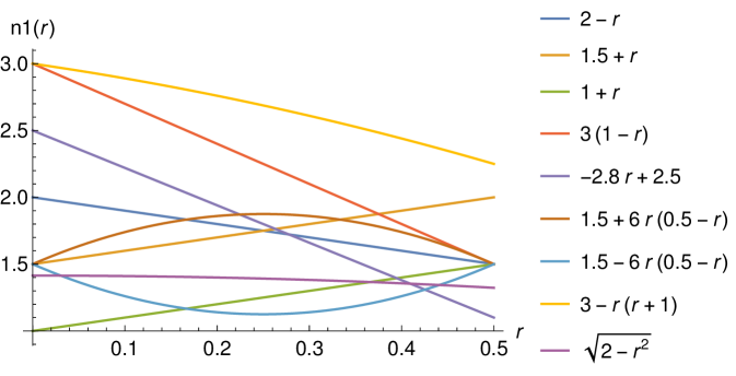
Figure 6: Different test cases in the non-constant case.

5.3.3 Interpretation of results

Based on the numerical experiments, the following observations can be made regarding the convergence of the Newton method presented in this Section 5.3.

Piecewise constant case:

• The Newton method converges for $n_{1}=1.5$ and $n_{2}=1$ (Table S-6), for all the considered $m\leq 60$ in a number of iterations $l\leq 9$. In high-contrast media however, e.g. $n_{1}=10$ and $n_{2}=1$ (Table S-7), the convergence of the Newton method may fail for high values of $m$ (starting from $m\geq 21$). There is thus a sensitivity of the Newton algorithm with respect to the jump in the refractive index $n^{2}$ at the interface (low/high-contrast media).

• It is worth noting, however, that even in the non-convergent cases (maximal number of iterations reached), the obtained $k$ is close to the corresponding theoretical asymptotic $k_{\mathrm{asympt}}$.

Variable case:

• The Newton method convergences in most of the considered cases using the same formula for the initial guess ($\frac{m}{\xi n_{1}(\xi)}$), except in some rare cases (Table S-17) where the maximal number of iterations can be reached for $m\geq 51$. We note that the imaginary part of the resonance in these cases approaches $0$ (values of order $1e{-}15/1e{-}17$). Nevertheless, as in the piecewise constant case, the obtained $k$ even in these “non-convergent” cases appears to be close to the corresponding theoretical asymptotic $k_{\mathrm{asympt}}$.

• We also note that the previous case, where the Newton method may fail to converge (Table S-17), corresponds to the case with the highest contrast in the refractive index at the interface (see Figure. 6).

• The considered example satisfying Thm. 1.C converges starting from $k_{0}=\frac{m}{\xi n_{1}(\xi)}$ (Table S-12) which is different from the leading term in the asymptotics in this case (which is $\frac{m}{\xi_{0}n_{1}(\xi_{0})}$ with $\xi_{0}=\frac{25}{56}\approx 0.44$, see Appendix D). Comparison with the the results obtained starting from $k_{\mathrm{asympt}}$ (Table S-14) gives comparable results for large $m$ that are also close to $k_{\mathrm{asympt}}$. Curiously enough, starting from the leading term $\frac{m}{\xi_{0}n_{1}(\xi_{0})}$ (Table S-13) gives different results for the resonances, that are quite far from $k_{\mathrm{asympt}}$. This shows a high sensitivity of the algorithm to the initial guess, especially in this case. In the other cases (Thm. 1.A or Thm. 1.B), the obtained resonances are close to $k_{\mathrm{asympt}}$ when starting from the leading term of the asymptotics ($k_{0}=\frac{m}{\xi n_{1}(\xi)}$ for these theorems). This difference of behavior for Thm. 1.C may be linked to the fact that quasi-resonances are not of whispering gallery type in this case: the quasi-modes are strictly localized inside the cavity (around $r=\xi_{0}<\xi$) [10].
  Nevertheless, this is a good point for our algorithm 2 where we specified the same initial guess independently of the verified theorem. This is particularly interesting when none of the theorems is valid (see next point).

• In the case of variable $n_{1}$ and $n_{2}$, theoretical asymptotic expansions are not available. In the considered cases (Tables S-19 and S-20), taking $n_{2}$ such that $n_{2}(\xi)=1$ and $n_{2}^{\prime}(\xi)=n_{2}^{\prime\prime}(\xi)=0$ (Table S-20) gives results that are close the the case $n_{2}=1$ (Table S-18), while a different variable $n_{2}$ satisfying only $n_{2}(\xi)=1$ (Table S-19) yields different results.

5.3.4 Quasi-resonance solutions and exact modes

After computing a resonance $k^{*}$, we can solve (30) for the quasi-resonance $k=\underline{k}=\Re(k^{*})$ and plot the solution $\hat{u}_{m}(r)$ (29) and $\Re[\hat{u}_{m}(r)e^{im\theta}]$ in Figure 8. We observe that they concentrate around the interface $r=\xi$ as $m$ gets large ($\Im(k^{*})$ gets closer to $0$). In Figure 7, we represented the norm $\|(T^{m}(k))^{-1}\|_{2}$ with respect to $k$ for the different values of $m$ considered: we observe spikes in this norm when $k$ is a quasi-resonance, since the matrix is close to being singular in this case ($\det(T^{m}(\underline{k}))\approx\det(T^{m}(k^{*}))=0$).

We can also plot the exact modes for a given resonance $k^{*}$: they are given, up to a complex multiplicative constant by,

$$u(r)=\begin{dcases}\frac{f_{1,1,k^{*}}(r)}{f_{1,1,k^{*}}(\xi)}&r\in(0,\xi)\\ \frac{f_{2,2,k^{*}}(r)}{f_{2,2,k^{*}}(\xi)}&r\in(\xi,1)\end{dcases}\quad\text{ or }\quad u(r)=\begin{dcases}\frac{f_{1,1,k^{*}}(r)}{f^{\prime}_{1,1,k^{*}}(\xi)}&r\in(0,\xi)\\ \frac{f_{2,2,k^{*}}(r)}{f^{\prime}_{2,2,k^{*}}(\xi)}&r\in(\xi,1),\end{dcases}$$ (98)

see Proposition 12.

The exact modes are shown in Figure 9 for the Luneburg case (see Table S-18), exhibiting the same localization behavior at the interface for large $m$ as the “quasi-modes” in Figure 8.

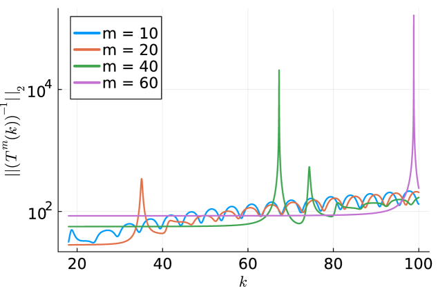
Figure 7: Plot of $\|(T^{m}(k))^{-1}\|_{2}$ with respect to $k$ for different values of $m$, in the Luneburg case $n_{1}(r)=\sqrt{2-r^{2}}$, $n_{2}(r)=1$ and $\xi=0.5$. Here $h_{1,1,k}=h_{2,2,k}=1$.

6 Comparison to other methods

As the resonance problem is expressed as a nonlinear eigenvalue problem (24), alternative techniques like the contour integral method [11, 9] or rational approximation [14, 52, 23] may be applied. We decided to develop and investigated the Newton approach because of its simplicity and its low number of control parameters. A major advantage of a Newton-type method over other nonlinear eigenvalue problem solution approaches is that the choice of an initial guess is usually the only crucial parameter. However, it could be worthwhile to assess the performance of several approaches using a benchmark for our particular situation, particularly in cases when the Newton technique does not appear to converge. Further research in this area may be pursued.

In Figures S-1 and S-2, we reported some first experiments with the NEP-Package [32]. As can be shown, the results are quite sensitive and require a detailed investigation given the different contour integration method parameters, for example. Furthermore, the Chebyshev interpolation introduces an extra error.

In the low-contrast case (Figure S-1) we recover the resonance obtained by our Newton method, using Quasi-Newton and Contour integral method for a good choice of parameters, while in the high-contrast case (Figure S-2), these methods seem to become non-robust to compute an adequate approximation of a resonance. We performed the test for $n_{1}=5$, $n_{2}=1$, $\xi=0.5$ and $m=21$ for which our Newton algorithm diverges (Table S-7).

7 Conclusion and outlook

In this paper, we have considered the problem of computing quasi-resonances in spherical symmetric heterogeneous Helmholtz problems with piecewise smooth refractive index. We have developed a general approach based on the splitting of the problem into decoupled problems on each domain and one problem at the interface (skeleton). In the spherical symmetric setting, we have reduced the problem to one-dimensional Sturm-Liouville problems. Using fundamental solutions, the problem of resonances is expressed as a nonlinear eigenvalue problem $T(k)x=0$ involving the values of the fundamental solutions and their derivatives at the interface. We then developed a numerical approach using Newton’s method to solve the nonlinear equation $\det(T(k))=0$ where the fundamental solutions and their derivatives are approximated numerically at each iteration. In the piecewise constant case, we prove the simplicity of the roots, providing a local quadratic convergence of the algorithm. In the variable case, we have specified the initial guess based on known asymptotic expansions, and suggested a proper scaling for the fundamental system in analogy with the piecewise constant case. Various numerical experiments, investigating the convergence and comparing the results to explicit solutions or asymptotic expansions, validate the results and our methodology. Perspectives include comparing the Newton method with other approaches developed for nonlinear eigenvalue problems, and investigating the extension of this method to more general settings following for instance [5, 6, 4]. It would also be interesting to consider a piecewise smooth refractive index with $p$ jump points as in [53], for its potential relevance in physical applications [12, 38].

Acknowledgements.

Part of the research was carried out while the first author was visiting the Institut für Mathematik at the University of Zürich as part of the CIMPA-ICTP Fellowship 2024 “Research in Pairs”. The first author thanks CIMPA and ICTP for the grant and the Institut für Mathematik for the hospitality. We thank Monique Dauge, Andrea Moiola and Zoïs Moitier for helpful discussions on WGM at the WAVES 2024 conference, and for pointing out the simplicity of eigenvalues for Sturm-Liouville problems.

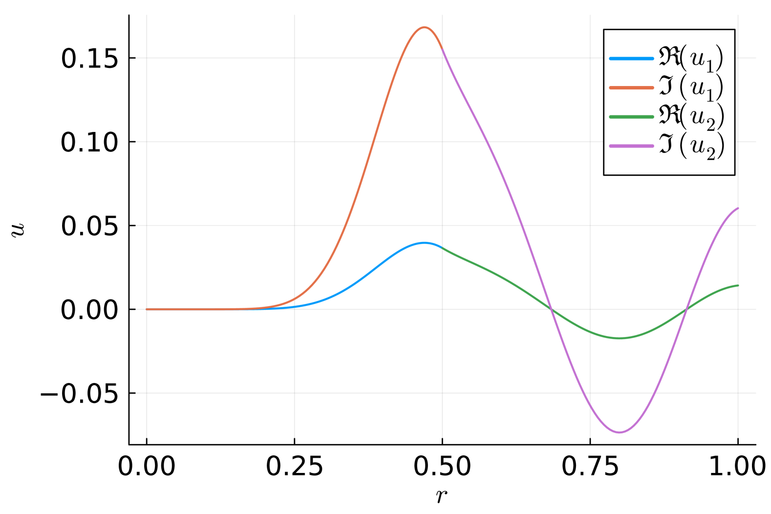
(a) $m=10$, $k=18.588964551092495$

(b) $m=20$, $k=35.094086477222184$

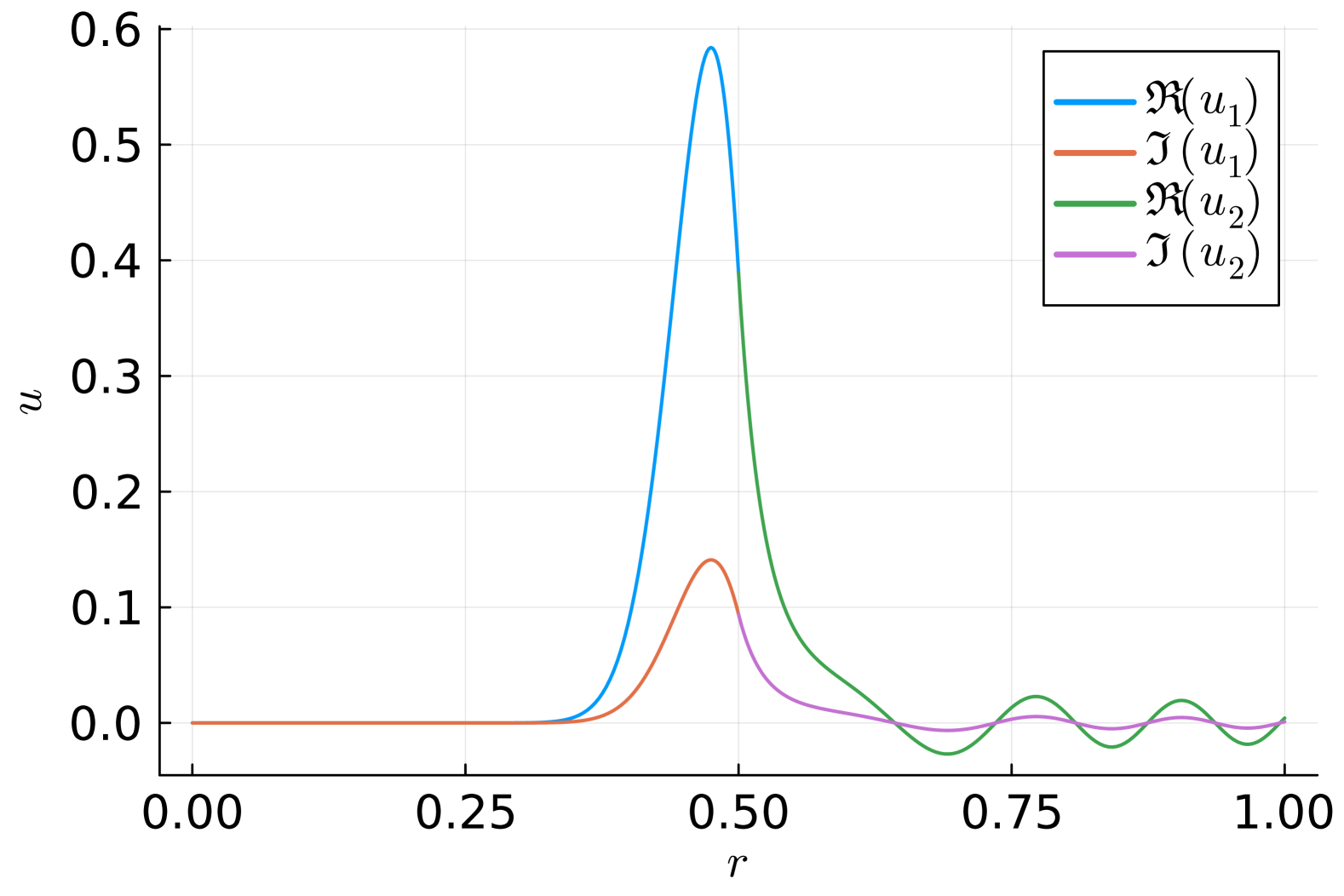
(c) $m=40$, $k=67.28740154078255$

(d) $m=60$, $k=98.82822050753336$

(e) Case (a)

(f) Case (b)

(g) Case (c)

(h) case (d)

Figure 8: (a)-(d): Plots of $\Re(\hat{u}_{m}(r))$ and $\Im(\hat{u}_{m}(r))$; (e)-(h): Polar plots of $\Re[\hat{u}_{m}(r)e^{im\theta}]$, for $\hat{u}_{m}(r)$ solution of (7) in the Luneburg case $n_{1}(r)=\sqrt{2-r^{2}}$, $n_{2}(r)=1$ and $\xi=0.5$, where $k$ is a quasi-resonance (close to a resonance), see Table S-18. Here $\hat{g}_{m}=1$.

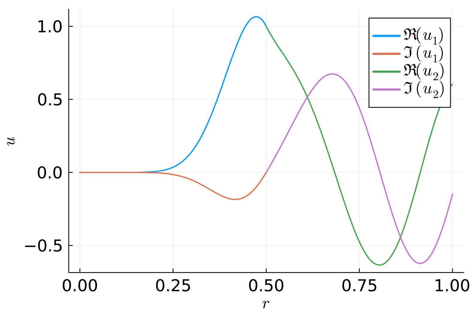
(a) $m=10$, $k=18.588964551092495-0.6154431006782064\,i$

(b) $m=20$, $k=35.094086477222184-0.19327141896886588\,i$

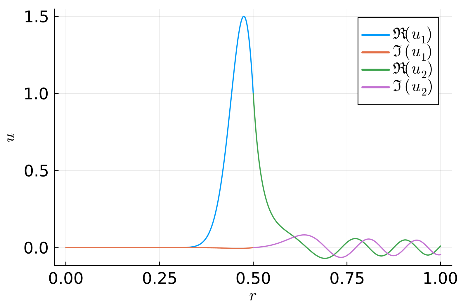
(c) $m=40$, $k=67.28740154078255-0.008096418587892958\,i$

(d) $m=60$, $k=98.82822050753336-0.0001666862148301293\,i$

(e) Case (a)

(f) Case (b)

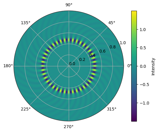
(g) Case (c)

(h) Case (d)

Figure 9: (a)-(d): Plots of $\Re(\hat{u}_{m}(r))$ and $\Im(\hat{u}_{m}(r))$; (e)-(h): Polar plots of $\Re[\hat{u}_{m}(r)e^{im\theta}]$, for the exact mode $\hat{u}_{m}(r)$ (98) solution of (7) for $\hat{g}_{m}=0$, where $k$ is a resonance, in the Luneburg case $n_{1}(r)=\sqrt{2-r^{2}}$, $n_{2}(r)=1$ and $\xi=0.5$, see Table S-18.

Appendix A Additional figures

$l$	$k_{l}$	$|\det_{1}(k_{l})|$	$|\partial_{k}\det_{1}(k_{l})|$
1	15.2027551239541 - 0.0014194570359291362im	4.671978949450817	3.3478557431073406
2	16.595070718259585 - 0.09584456745332563im	0.766528533057148	2.262222095143523
3	16.910865265369715 - 0.21866765298920093im	0.04904518069884701	2.025095495385794
4	16.92329111475096 - 0.2394557194458im	0.00025583057039584825	2.0197612390638997
5	16.923201859904534 - 0.239545593149898im	7.0104524408116925e-9	2.019858377921107

(a) $\det_{1}$ starting from $k_{0}=11$.

$l$	$k_{l}$	$|\det_{2}(k_{l})|$	$|\partial_{k}\det_{2}(k_{l})|$
1	13.396229610406712 + 4.6308732874575025im	0.03278374907593669	0.0036291583324786726
2	21.37329855682114 + 8.869886753253347im	0.01810878631760116	0.0007994486471827419
3	42.399466900838604 + 17.295737648975493im	0.009111967034763104	0.00019960877192767506
4	84.49957023255998 + 34.942960837304014im	0.004557282325858091	4.988028897511637e-5
5	168.80515382942275 + 70.15689112416922im	0.0022790096173500697	1.2467869613546143e-5
6	337.50591933464125 + 140.53062554154792im	0.0011395611271406746	3.1168082028382702e-6
7	674.9581092588107 + 281.25208333979583im	0.0005697881858075883	7.791914716934638e-7
8	1349.8889995007594 + 562.6826361056818im	0.0002848950810892208	NaN

(b) $\det_{2}$ starting from $k_{0}=11$.

$l$	$k_{l}$	$|\det_{1}(k_{l})|$	$|\partial_{k}\det_{1}(k_{l})|$
1	16.933172576735238 - 0.24982842615297063im	0.02888927214377845	2.014089202013235
2	16.92321608496663 - 0.23950336537694566im	8.999610742390703e-5	2.01983595147453
3	16.92320186112372 - 0.23954559016258034im	8.674673679574019e-10	2.0198583761562476

(c) $\det_{1}$ starting from $k_{0}=17$.

$l$	$k_{l}$	$|\det_{2}(k_{l})|$	$|\partial_{k}\det_{2}(k_{l})|$
1	16.903562544030315 - 0.2594084783861693im	0.0005849587965634079	0.021077843582846287
2	16.922896121039905 - 0.2394985971301382im	6.435727667618858e-6	0.020804555113225907
3	16.92320187831679 - 0.2395455557149322im	7.969831186777102e-10	0.020806177812095424

(d) $\det_{2}$ starting from $k_{0}=17$.

Table 3: Newton iterations using $\det_{1}$ or $\det_{2}$ for $\xi=0.5$, $n_{1}=1.5$, $n_{2}=1$ and $m=10$, starting from $k_{0}=11$ or $k_{0}=17$.

Appendix B Complex plots of different scalings of the determinant

As explained in Section 4.2.5, different choices of $h_{1,1,k}$ and $h_{2,2,k}$ lead to different scalings of the fundamental solutions and hence to different scalings of the determinant. In the piecewise constant case, we denote the determinant (when defined) obtained for $h_{1,1,k}=\frac{1}{c_{1,k}}$ and $h_{2,2,k}=\frac{1}{c_{2,k}}$ by

$$\mathrm{det}_{1}(k)=k[n_{1}J_{m}^{\prime}(kn_{1}\xi)H_{m}(kn_{2}\xi)-n_{2}J_{m}(kn_{1}\xi)H_{m}^{\prime}(kn_{2}\xi)]$$ (99)

and the one obtained for $h_{1,1,k}=h_{2,2,k}=1$ by

$$\mathrm{det}_{2}(k)=c_{1,k}c_{2,k}\mathrm{det}_{1}(k),$$ (100)

so that

$$\frac{\partial_{k}\mathrm{det}_{2}(k)}{\mathrm{det}_{2}(k)}=\frac{\partial_{k}c_{1,k}}{c_{1,k}}+\frac{\partial_{k}c_{2,k}}{c_{2,k}}+\frac{\partial_{k}\mathrm{det}_{1}(k)}{\mathrm{det}_{1}(k)},$$ (101)

where, in the piecewise constant case,

$$\begin{dcases}c_{1,k}=\frac{1}{kn_{1}(J^{\prime}_{m}(kn_{1}\xi)-iJ_{m}(kn_{1}\xi))}\\ c_{2,k}=\frac{1}{-kn_{2}(H^{\prime}_{m}(kn_{2}\xi)+iH_{m}(kn_{2}\xi))}.\end{dcases}$$ (102)

We also consider

$$\mathrm{det}_{\mathrm{scal}}(k)=k^{2}\mathrm{det}_{2}(k).$$ (103)

In the following, we show complex plots of these different scalings of the determinant (Figures 11 and 12) and the involved quantities $c_{1,k}$ and $c_{2,k}$ (Figures 13). While the different determinants share the same zeros in ${\mathbb{C}}^{*}_{\geq 0}\cup({\mathbb{C}}_{<0}\setminus Z)$ where $Z$ is the set of the zeros of $\frac{1}{c_{1,k}}$ or $\frac{1}{c_{2,k}}$ (Remark 3), since (100) holds and $c_{1,k}$ and $c_{2,k}$ are different from zero in this set (see Lemmas 10 and 11), they may exhibit different behaviors which may affect the Newton algorithm.

The complex plots were made using the zplot function in Julia. The plots of $\mathrm{det}_{1}$ (Figure 11(a)) and $\log|\det_{1}|$ (Figure 11(c)) show as expected the organization of the zeros in two categories [10]: inner and outer resonances, for which the modes are essentially supported inside respectively outside the disk $B(0,\xi)$. Outer resonances satisfy $\Im(k)<\tau$ while inner ones satisfy $\Im(k)\geq\tau$ for a given negative threshold $\tau$. While the zeros of $\mathrm{det}_{2}$ are the same as those of $\mathrm{det}_{1}$ (when both are defined), it appears in the plots of $\mathrm{det}_{2}$ and $\log|\mathrm{det}_{2}|$ (Figures 11(b) and 11(d)), that the zeros have been polluted by the poles of $c_{1,k}$ or $c_{2,k}$ (Figures 13(a), 13(c), 13(b) and 13(d)). However, this should not explain the difference of behavior in the Newton algorithm since the plots for $\Im(k)<0$ can be misleading: the plotted $\det_{1}$ corresponds to the exact formula (99), while the constructed $\det_{1}$ from the auxiliary problems (23) is only defined outside $Z$ thus the constructed $\det_{1}$ also suffers from indetermination for $k\in Z$. The plots, however, have the merit of making one conjecture that the resonances are distinct from the poles of $c_{1,k}$ or $c_{2,k}$, hence that Assumption 6 is satisfied in the piecewise constant case.

Maybe the most important factor affecting the Newton method using the different scalings can be found in the plots of $\operatorname{sign}(\Im(\frac{\partial_{k}\det(k)}{\det(k)}))$ related to the phase of $\frac{\partial_{k}\det(k)}{\det(k)}$, extending the plot made on the real axis (Figure 3): one of the biggest advantages of $\det_{1}$ over the other scalings is that it could be conjectured form Figure 11(g) that the considered quantity is always negative for $\Im(k)\geq 0$, meaning that if a given iterate $k_{l}$ in the Newton algorithm is such that $\Im(k_{l})\geq 0$, then the next applications of the Newton algorithm will have a tendency to send it back to the region $\Im(k)<0$ where we are looking for zeros. The other scalings $\det_{2}$ (Figure 11(h)) and $\det_{\mathrm{scal}}$ (Figure 12(d)) lack this property, which could explain why for some starting points on the real axis, the next iterates could have their imaginary part that keeps increasing in the region $\Im(k)>0$ (case of $\det_{2}$ where a big region inside $\Im(k)>0$ have a wrong sign), or may have an oscillatory behavior in some sub-region $0<\Im(k)<\alpha$ where the plotted sign is not constant (case of both $\det_{2}$ and $\det_{\mathrm{scal}}$).

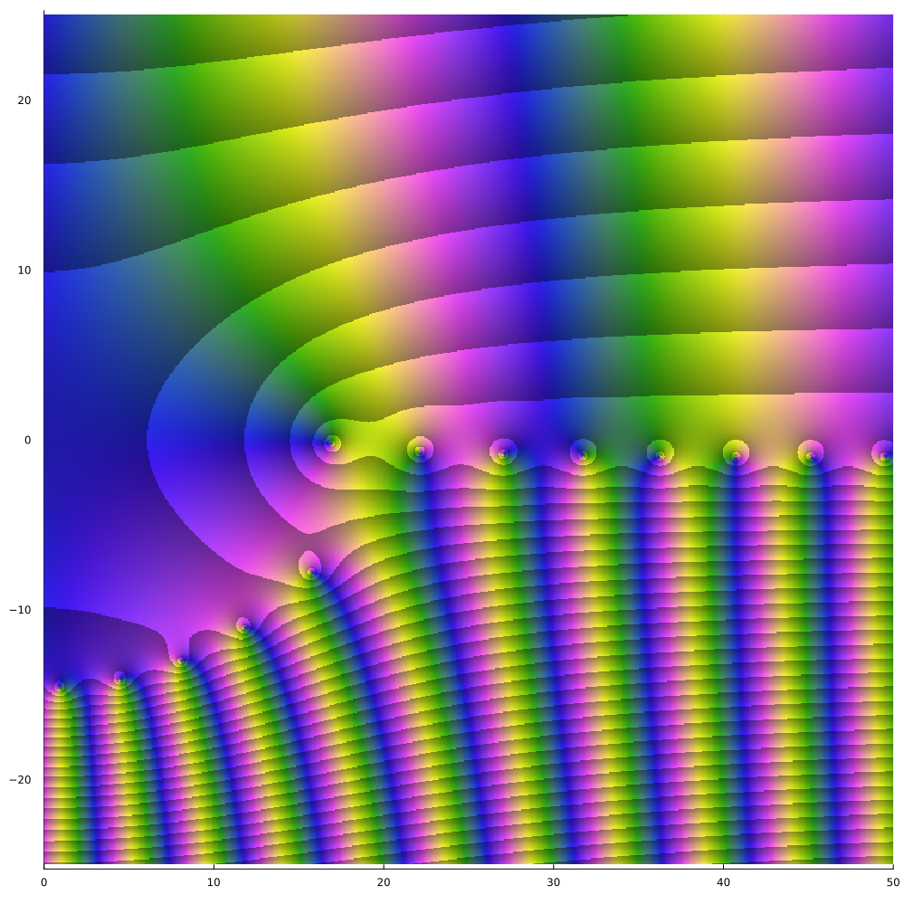
(a) $\det_{1}(k)$

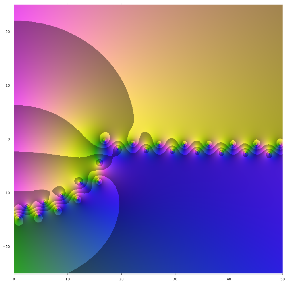
(b) $\det_{2}(k)$

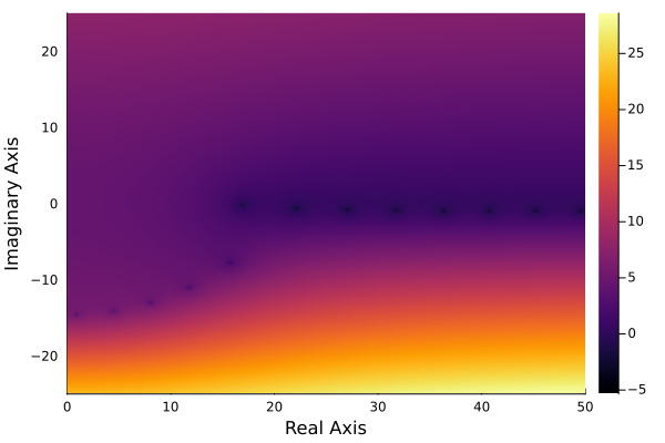
(c) $\log|\det_{1}(k)|$

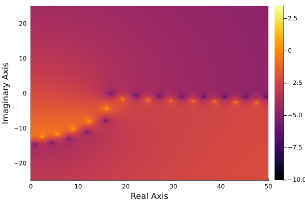
(d) $\log|\det_{2}(k)|$

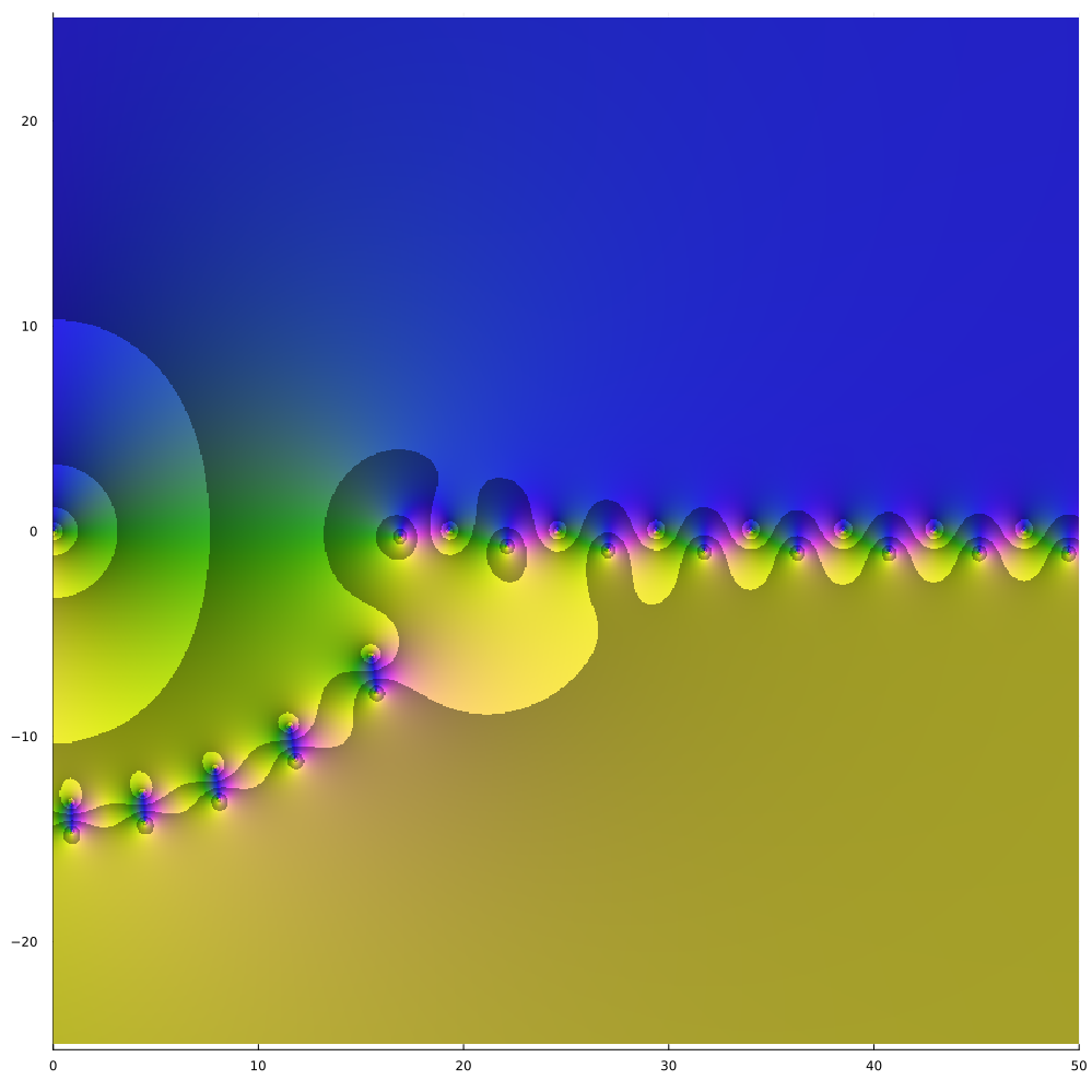
(e) $\frac{\partial_{k}\det_{1}(k)}{\det_{1}(k)}$

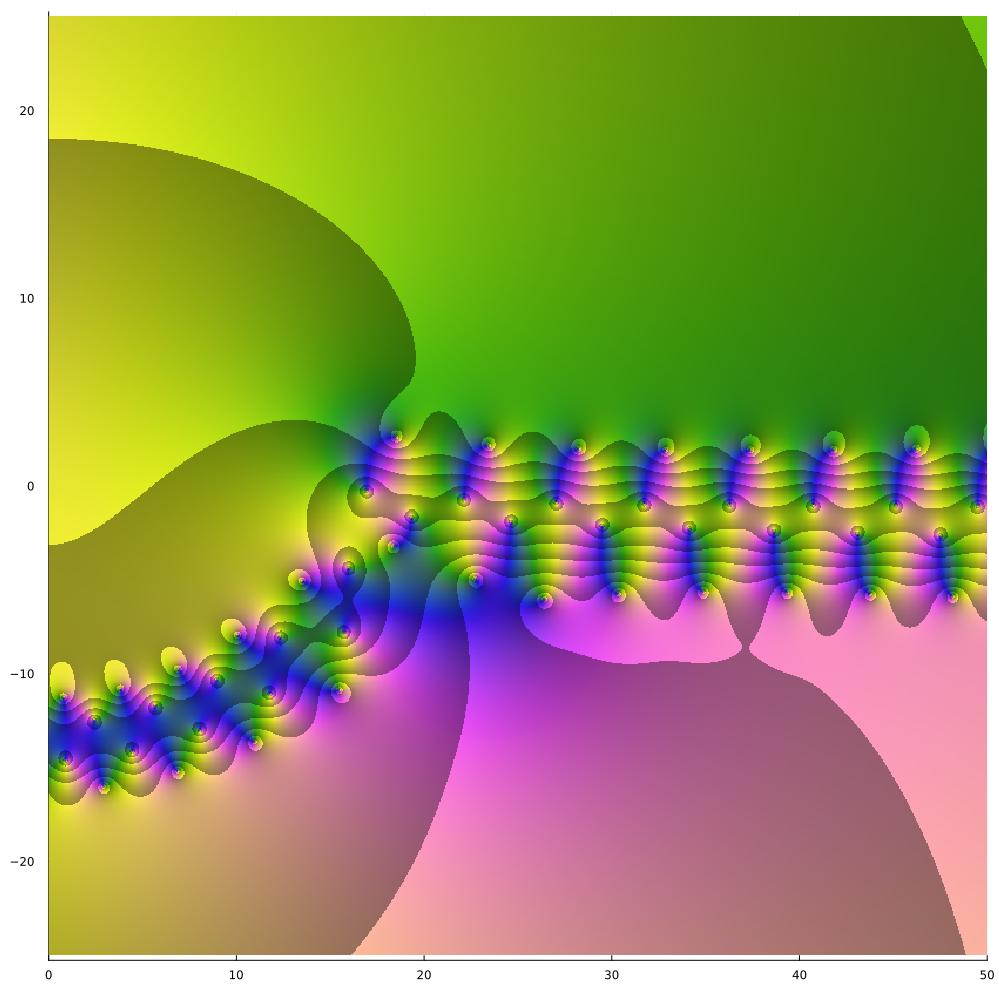
(f) $\frac{\partial_{k}\det_{2}(k)}{\det_{2}(k)}$

(g) $\operatorname{sign}(\Im(\frac{\partial_{k}\det_{1}(k)}{\det_{1}(k)}))$

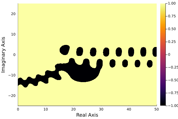
(h) $\operatorname{sign}(\Im(\frac{\partial_{k}\det_{2}(k)}{\det_{2}(k)}))$

Figure 11: Complex plots of $\det_{1}(k)$, $\det_{2}(k)$, $\frac{\partial_{k}\det_{1}(k)}{\det_{1}(k)}$ and $\frac{\partial_{k}\det_{2}(k)}{\det_{2}(k)}$ for $\xi=0.5$, $n_{1}=1.5$, $n_{2}=1$ and $m=10$.

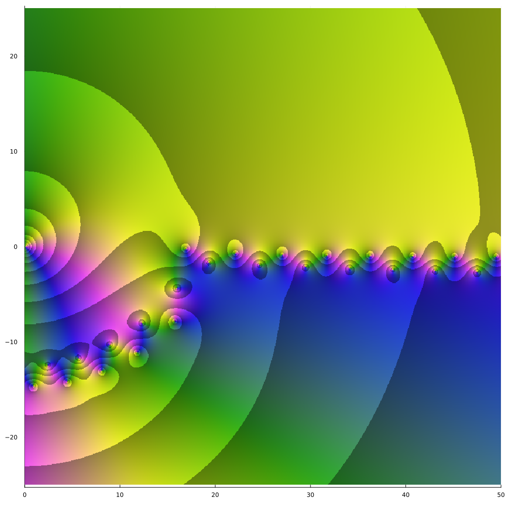
(a) $\det_{\mathrm{scal}}(k)$

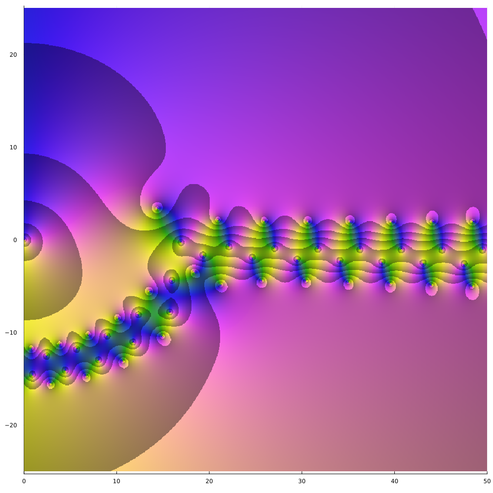
(b) $\frac{\partial_{k}\det_{\mathrm{scal}}(k)}{\det_{\mathrm{scal}}(k)}$

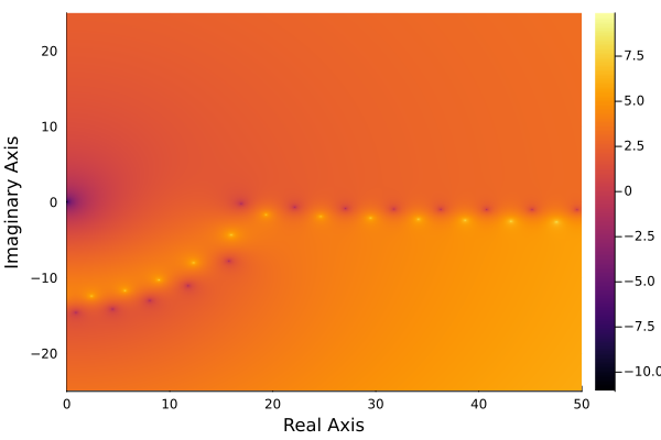
(c) $\log|\det_{\mathrm{scal}}(k)|$

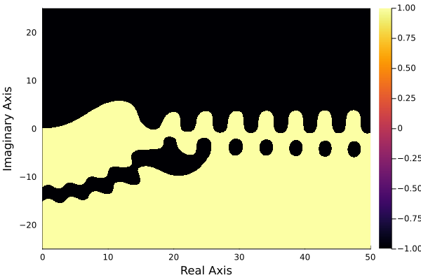
(d) $\operatorname{sign}(\Im(\frac{\partial_{k}\det_{\mathrm{scal}}(k)}{\det_{\mathrm{scal}}(k)}))$

Figure 12: Complex plots of $\det_{\mathrm{scal}}(k)$ and $\frac{\partial_{k}\det_{\mathrm{scal}}(k)}{\det_{\mathrm{scal}}(k)}$ for $\xi=0.5$, $n_{1}=1.5$, $n_{2}=1$ and $m=10$.

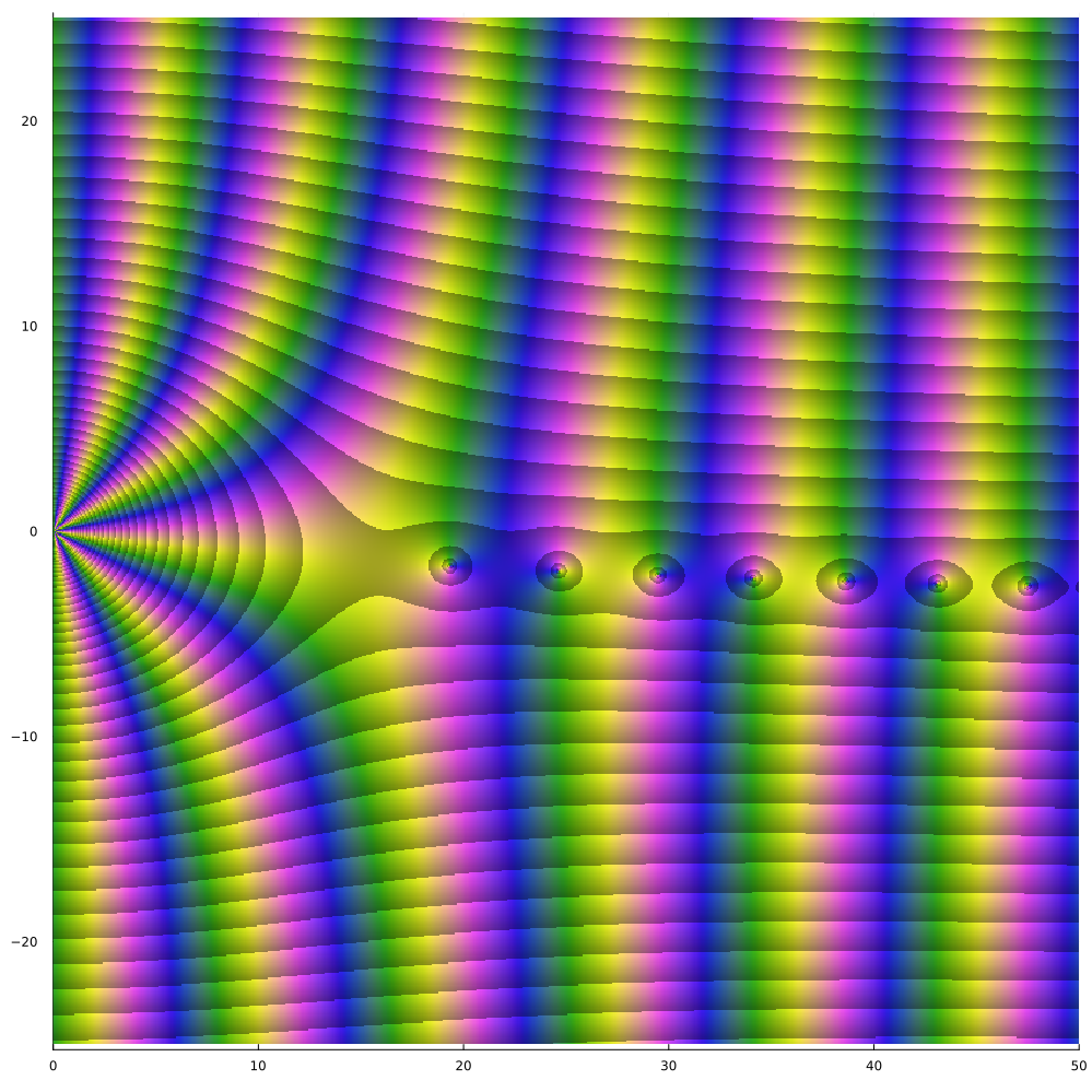
(a) $c_{1,k}$

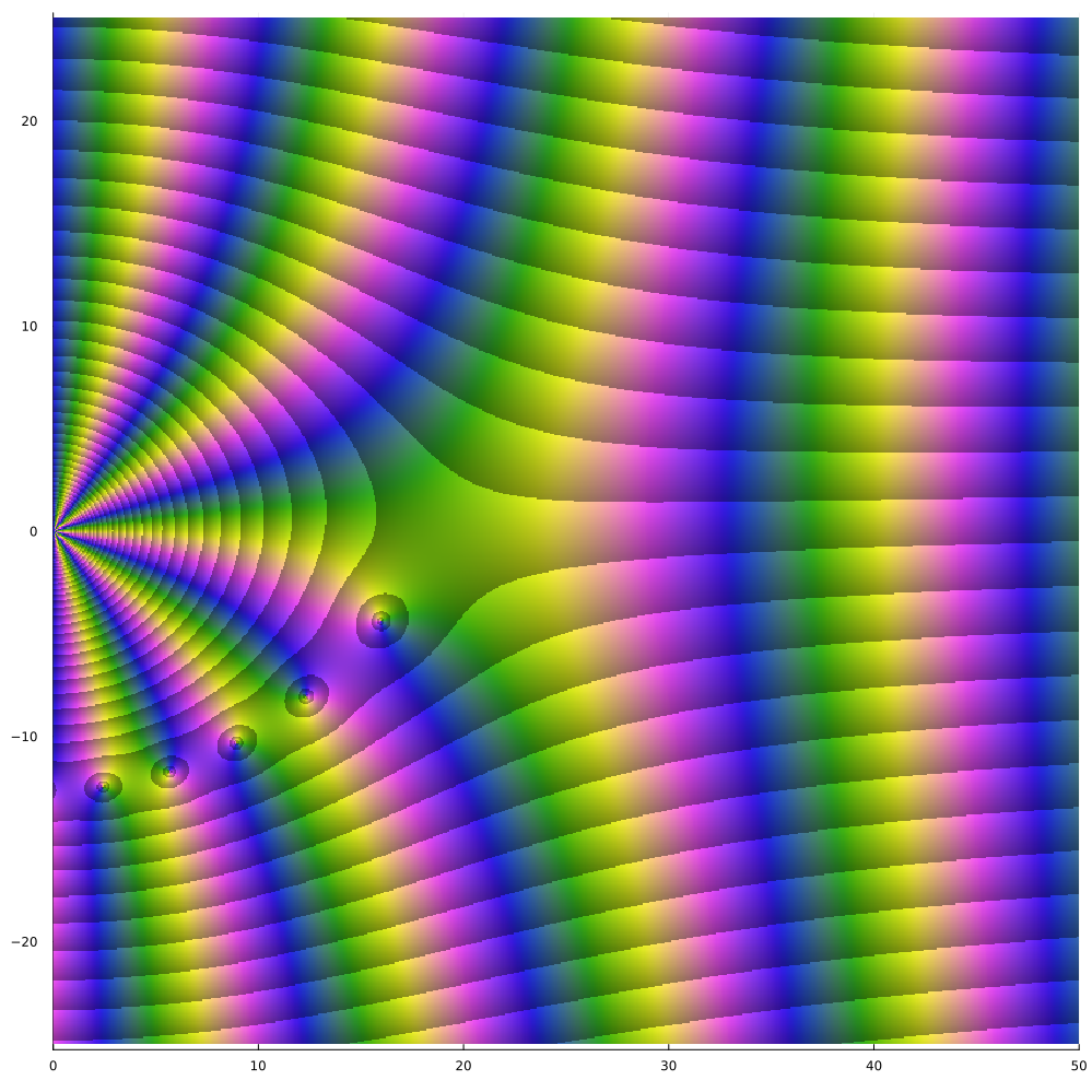
(b) $c_{2,k}$

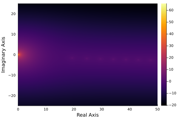
(c) $\log|c_{1,k}|$

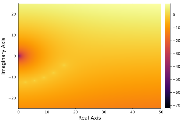
(d) $\log|c_{2,k}|$

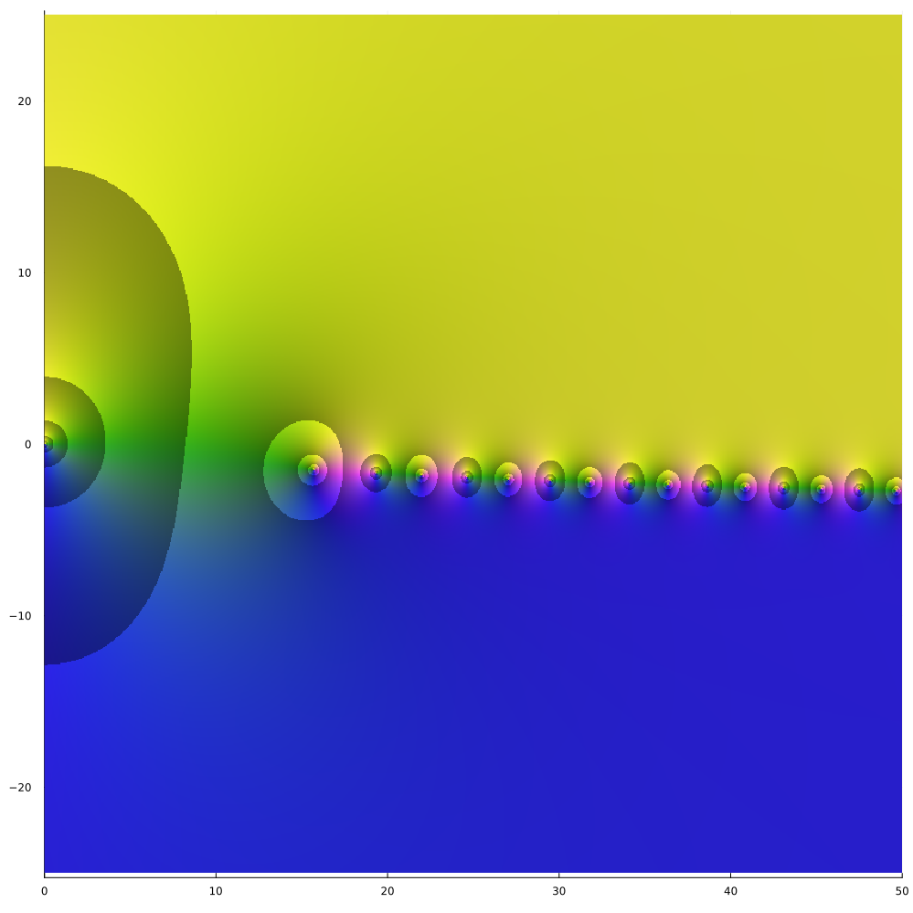
(e) $\frac{\partial_{k}c_{1,k}}{c_{1,k}}$

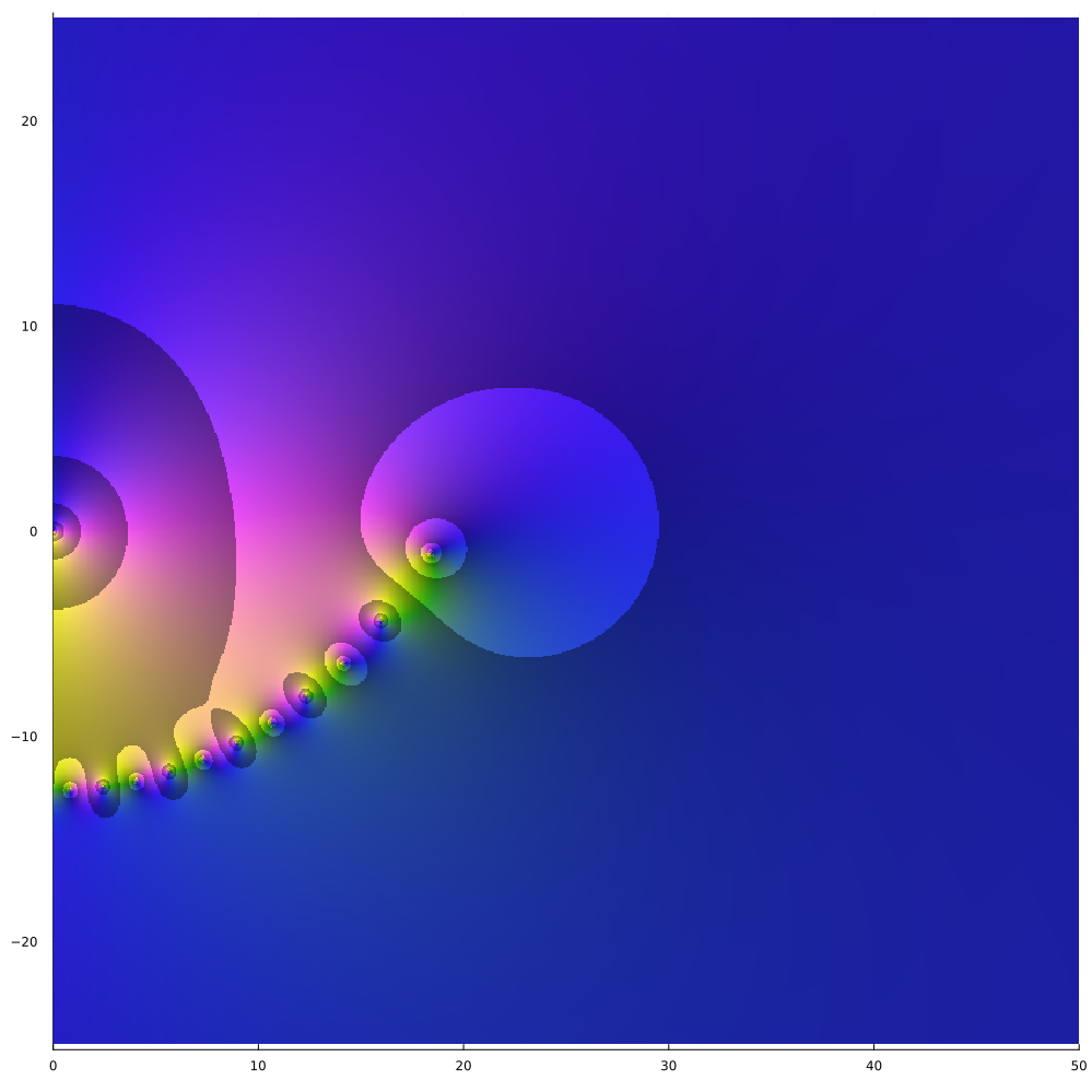
(f) $\frac{\partial_{k}c_{2,k}}{c_{2,k}}$

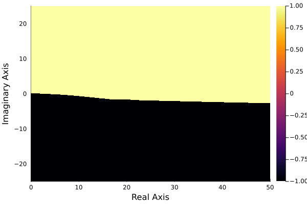
(g) $\operatorname{sign}(\Im(\frac{\partial_{k}c_{1,k}}{c_{1,k}}))$

(h) $\operatorname{sign}(\Im(\frac{\partial_{k}c_{2,k}}{c_{2,k}}))$

Figure 13: Complex plots of $c_{1,k}$, $c_{2,k}$, $\frac{\partial_{k}c_{1,k}}{c_{1,k}}$ and $\frac{\partial_{k}c_{2,k}}{c_{2,k}}$ for $\xi=0.5$, $n_{1}=1.5$, $n_{2}=1$ and $m=10$.

Appendix C Basic properties of nonlinear eigenvalue problems [58]

We gather here some definitions and basic properties of nonlinear eigenvalue problems.

We consider the problem of finding $\lambda$ such that the linear system

$$T(\lambda)x=0$$ (104)

has a nontrivial solution $x$, where $T(.)\colon D\to{\mathbb{C}}^{n\times n}$ is a family of matrices depending on a complex parameter $\lambda\in D$.

Definitions:

$\hat{\lambda}\in D$ is called an eigenvalue of $T(\cdot)$ if $T(\hat{\lambda})x=0$ has a nontrivial solution $\hat{x}\neq 0$. $\hat{x}$ is called a corresponding eigenvector or right eigenvector, and $(\hat{\lambda},\hat{x})$ is called eigenpair of $T(\cdot)$.

Any nontrivial solution $\hat{y}\neq 0$ of the adjoint equation $T(\hat{\lambda})^{*}y=0$ is called left eigenvector of $T(\cdot)$ and the vector-scalar-vector triplet $(\hat{y},\hat{\lambda},\hat{x})$ is called an eigentriplet of $T(\cdot)$.

An eigenvalue $\hat{\lambda}$ of $T(\cdot)$ has algebraic multiplicity $k$ if $\frac{d^{\ell}}{d\lambda^{\ell}}\det{(T(\lambda))}|_{\lambda=\hat{\lambda}}=0$ for $\ell=0,\ldots,k-1$ and $\frac{d^{k}}{d\lambda^{k}}\det{(T(\lambda))}|_{\lambda=\hat{\lambda}}\neq 0$.

An eigenvalue $\hat{\lambda}$ is simple if its algebraic multiplicity is one.

The geometric multiplicity of an eigenvalue $\hat{\lambda}$ is the dimension of the kernel $\ker(T(\hat{\lambda}))$ of $T(\hat{\lambda})$.

An eigenvalue is called semi-simple if its algebraic and geometric multiplicity coincide.

Properties:

If $\hat{\lambda}$ is an algebraically simple eigenvalue of $T(\cdot)$, then $\hat{\lambda}$ is geometrically simple. [54]

Let $(\hat{y},\hat{\lambda},\hat{x})$ be an eigentriplet of $T(\cdot)$. Then $\hat{\lambda}$ is algebraically simple if and only if $\hat{\lambda}$ is geometrically simple and $\hat{y}^{*}T^{\prime}(\hat{\lambda})\hat{x}\neq 0$. [43, 54]

Appendix D Asymptotic expansions of quasi-resonances in dimension 2 [10]

We gather here some of the results in [10] regarding the construction of quasimodes $(\underline{k}(m),\underline{u}(m))$ as $m\to\infty$, i.e. approximate solutions of (7) with $\hat{g}_{m}=0$, in three different configurations. Moreover, it is shown in [10] that the constructed quasi-resonances $\underline{k}_{j}(m)$ are real and positive and close to true resonances $k_{j}(m)$ modulo a super-algebraic error $O(m^{-\infty})$.

Assumption 1.1.

The radial function $n\colon r\mapsto n(r)$ satisfies the following properties:

1. $n(r)=1$ if $r>\xi$ ;

2. The function $n$ belongs to $C^{\infty}([0,\xi])$ and $n(r)>1$ for all $r\leq\xi$.

Notation 1.2.

$$n_{0}=\lim\limits_{r\nearrow\xi}n(r),\quad n_{I}=\lim\limits_{r\nearrow\xi}n^{\prime}(r),\quad n_{II}=\lim\limits_{r\nearrow\xi}n^{\prime\prime}(r).$$ (105)

Effective adimensional curvature:

$$\check{\kappa}:=\xi\Bigl{(}\frac{1}{\xi}+\frac{n_{I}}{n_{0}}\Bigr{)}.$$ (106)

Adimensional Hessian:

$$\check{\mu}:=\xi^{2}\Bigl{(}\frac{2}{\xi^{2}}-\frac{n_{II}}{n_{0}}\Bigr{)}.$$ (107)

Theorem 1.A.

Assume the radial function $n$ satisfies Assumption 1.1 and

$$\check{\kappa}>0.$$ (108)

Then, for any integer $j\geq 0$, there exists a quasi-pair $(\underline{k}_{j}(m),\underline{u}_{j}(m))$ such that the quasi-resonance $\underline{k}_{j}(m)$ has an expansion in integer powers of $m^{-1/3}$ starting as

$$\underline{k}_{j}(m)=\frac{m}{\xi n_{0}}\Bigl{[} 1+\frac{a_{j}}{2}\Bigl{(}\frac{2\check{\kappa}}{m}\Bigr{)}^{\frac{2}{3}}-\frac{n_{0}}{2\sqrt{n_{0}^{2}-1}}\Bigl{(}\frac{2\check{\kappa}}{m}\Bigr{)}+\frac{a_{j}^{2}}{15}\Bigl{(}\frac{17}{8}-\frac{3}{\check{\kappa}}+\frac{\check{\mu}}{\check{\kappa}^{2}}\Bigr{)}\Bigl{(}\frac{2\check{\kappa}}{m}\Bigr{)}^{\frac{4}{3}}$$

$$\quad-\frac{a_{j}n_{0}}{12\sqrt{n_{0}^{2}-1}}\Bigl{(}\frac{n_{0}^{2}}{n_{0}^{2}-1}+2-\frac{6}{\check{\kappa}}+\frac{2\check{\mu}}{\check{\kappa}^{2}}\Bigr{)}\Bigl{(}\frac{2\check{\kappa}}{m}\Bigr{)}^{\frac{5}{3}}+O(m^{-2})\Bigr{]}$$ (109)

with the numbers $a_{j}$ being the successive roots of the flipped Airy function $z\in{\mathbb{C}}\mapsto\mathrm{Ai}(-z)$ where $\mathrm{Ai}$ denotes the Airy function [1, 19].

Theorem 1.B.

Assume the radial function $n$ satisfies Assumption 1.1 and

$$\check{\kappa}=0\quad\text{with}\quad\check{\mu}>0.$$ (110)

Then, for any integer $j\geq 0$, there exists a quasi-pair $(\underline{k}_{j}(m),\underline{u}_{j}(m))$ such that the quasi-resonance $\underline{k}_{j}(m)$ has an expansion in integer powers of $m^{-1/2}$ starting as

$$\underline{k}_{j}(m)=\frac{m}{\xi n_{0}}\Bigl{[}1+\frac{4j+3}{2}\Bigl{(}\frac{\sqrt{\check{\mu}}}{m}\Bigr{)}+O(m^{-\frac{3}{2}})\Bigr{]},$$ (111)

the coefficient of degree $1$ being zero.

Theorem 1.C.

Assume the radial function $n$ satisfies Assumption 1.1 and that

$$\check{\kappa}<0.$$ (112)

Let $\xi_{0}\in(0,\xi)$ such that $1+\frac{\xi_{0}n^{\prime}(\xi_{0})}{n(\xi_{0})}=0$ and assume further that

$$\check{\mu}_{0}:=\xi_{0}^{2}\Bigl{(}\frac{2}{\xi_{0}^{2}}-\frac{n^{\prime\prime}(\xi_{0})}{n(\xi_{0})}\Bigr{)}>0.$$ (113)

Then, for any integer $j\geq 0$, there exists a quasi-pair $(\underline{k}_{j}(m),\underline{u}_{j}(m))$ such that the quasi-resonance $\underline{k}_{j}(m)$ has an expansion in integer powers of $m^{-1/2}$ starting as

$$\underline{k}_{j}(m)=\frac{m}{\xi_{0}n(\xi_{0})}\Bigl{[}1+\frac{2j+1}{2}\Bigl{(}\frac{\sqrt{\check{\mu}_{0}}}{m}\Bigr{)}+O(m^{-2})\Bigr{]},$$ (114)

the coefficients of degree $1$ and $3$ being zero.

Appendix E Special variable $n$ with explicit solution (Luneburg lens)

The fundamental solutions of the second-order differential equation

$$-y^{\prime\prime}(x)-\frac{y^{\prime}(x)}{x}+\Bigl{(}\frac{m^{2}}{x^{2}}-k^{2}(2-x^{2})\Bigr{)}y(x)=0$$ (115)

(where $n(x)=\sqrt{2-x^{2}}$) are given by

• $\displaystyle f_{1}(x)=\frac{1}{x}M_{\frac{k}{2},\frac{m}{2}}(kx^{2})$ (vanishes at $x=0$)

• $\displaystyle f_{2}(x)=\frac{1}{x}W_{\frac{k}{2},\frac{m}{2}}(kx^{2})$ (singular at $x=0$)

where $M_{k,m}(z)$ and $W_{k,m}(z)$ are the Whittaker functions [1, 60, 44], solutions of the Whittaker differential equation

$$w^{\prime\prime}+\Big{(}\frac{1/4-m^{2}}{z^{2}}+\frac{k}{z}-\frac{1}{4}\Bigr{)}w=0.$$ (116)

Indeed, if one looks for a solution of (115) in the form $y(x)=\frac{1}{x}w(kx^{2})$ then using

$$y^{\prime}(x) =2kw^{\prime}(kx^{2})-\frac{1}{x^{2}}w(kx^{2})$$ (117)

$$y^{\prime\prime}(x) =4k^{2}xw^{\prime\prime}(kx^{2})-\frac{2k}{x}w^{\prime}(kx^{2})+\frac{2}{x^{3}}w(kx^{2}),$$ (118)

the differential equation (115) becomes

$$-4k^{2}xw^{\prime\prime}(kx^{2})-\Bigl{(}\frac{1-m^{2}}{x^{3}}+\frac{k^{2}(2-x^{2})}{x}\Bigr{)}w(kx^{2}) =0$$ (119)

$$w^{\prime\prime}(kx^{2})+\Bigl{(}\frac{1-m^{2}}{4k^{2}x^{4}}+\frac{1}{2x^{2}}-\frac{1}{4}\Bigr{)}w(kx^{2}) =0,$$ (120)

hence the announced result.

We have used the Whittaker representation in our implementation for its convenience and reduced form.

This special case in linked to the Luneburg lens which is a spherically symmetric gradient-index lens, whose typical refractive index has the same form considered here [12, 36, 37, 38].

Supplementary Material: Computation of whispering gallery modes for spherical symmetric heterogeneous Helmholtz problems with piecewise smooth refractive index
Bouchra Bensiali and Stefan Sauter

Contents

1. 1 Introduction
2. 2 Problem formulation
   1. 2.1 Polar coordinates and fundamental systems
   2. 2.2 Well-posedness of ODEs for the fundamental system
   3. 2.3 Quasi-resonances
3. 3 A Newton method for determining critical $k$’s
   1. 3.1 Newton’s algorithm
   2. 3.2 Starting values
   3. 3.3 Local convergence
4. 4 Piecewise constant case
   1. 4.1 Convergence of the Newton method: simplicity of the roots
   2. 4.2 Experiments
      1. 4.2.1 Computation of zeros
      2. 4.2.2 Verifying $\Im(k_{m,j})<\Im(k_{m,1})<0$ for $j>1$
      3. 4.2.3 Verifying $\Im(k_{m,1})\underset{m\to\infty}{\longrightarrow}0$
      4. 4.2.4 Verifying $\Im(k_{m,1}(n_{1}))<0$ is a non-decreasing function of $n_{1}$ for $n_{1}>n_{2}=1$
      5. 4.2.5 Choice of $h_{1,1,k}$ and $h_{2,2,k}$: proper conditioning
5. 5 Variable case
   1. 5.1 Convergence of the Newton method: simplicity of the roots (see definition in Appendix C)
      1. 5.1.1 Geometric simplicity
      2. 5.1.2 Algebraic simplicity
   2. 5.2 Experiments
      1. 5.2.1 Using ApproxFun to solve Bessel-type equations
      2. 5.2.2 Newton method using ApproxFun
         1. 5.2.2.1 Constant case validation
         2. 5.2.2.2 Variable cases validation
            1. 5.2.2.2.1 A perturbation of a constant by a bump function
            2. 5.2.2.2.2 A special variable case with explicit solution
   3. 5.3 Newton method for variable refractive index
      1. 5.3.1 Piecewise constant cases
      2. 5.3.2 Non-constant cases (illustrated in Fig. 6)
      3. 5.3.3 Interpretation of results
      4. 5.3.4 Quasi-resonance solutions and exact modes
6. 6 Comparison to other methods
7. 7 Conclusion and outlook
8. A Additional figures
9. B Complex plots of different scalings of the determinant
10. C Basic properties of nonlinear eigenvalue problems [58]
11. D Asymptotic expansions of quasi-resonances in dimension 2 [10]
12. E Special variable $n$ with explicit solution (Luneburg lens)
13. S1 Constant case validation
14. S2 Variable cases validation
    1. S2.1 A perturbation of a constant by a bump function
    2. S2.2 A special variable case with explicit solution (Luneburg lens)
15. S3 Piecwise constant cases
    1. S3.1 Low-contrast media
    2. S3.2 High-contrast media
16. S4 Variable cases
    1. S4.1 $n_{1}$ variable and $n_{2}=1$
    2. S4.2 $n_{1}$ and $n_{2}$ variable
17. S5 Comparison to other methods

Appendix S1 Constant case validation

$k_{0}$	—$l$—	—$k$—	—$|D(k)|$—	—$|\partial_{k}D(k)|$—
1	10	16.92320186058385 -0.23954559046213897 I	$8.431690394646775*10^{-11}$	0.11934243142749136
	10	16.923201860583823 - 0.23954559046216217im	8.432518900901111e-11	0.11934243142750814
2	9	16.923201860607477 -0.239545590346429 I	$7.062130338578378*10^{-11}$	0.11934243142433129
	9	16.923201860607584 - 0.23954559034648804im	7.061816901668366e-11	0.11934243142431934
3	8	16.923201958814623 -0.23954567846387156 I	$1.5765662917540812*10^{-8}$	0.11934242645677033
	8	16.92320195881486 - 0.2395456784639192im	1.576569118232158e-8	0.1193424264567462
4	8	16.923201860703298 -0.2395455900407501 I	$3.338609990317884*10^{-11}$	0.11934243141380349
	8	16.923201860703177 - 0.23954559004071005im	3.3386019946832795e-11	0.11934243141380377
5	7	16.92320302561573 -0.23954583736498444 I	$1.4210835156091535*10^{-7}$	0.11934236091527006
	7	16.923203025615667 - 0.2395458373649745im	1.4210833444854101e-7	0.11934236091525743
6	7	16.923201876723557 -0.2395456186602138 I	$3.928006210547949*10^{-9}$	0.1193424308101149
	7	16.923201876723734 - 0.23954561866023547im	3.928027387263182e-9	0.11934243081007889
7	7	16.9232018606048 -0.23954559035873113 I	$7.207125317039786*10^{-11}$	0.11934243142466965
	7	16.923201860604816 - 0.23954559035875164im	7.207734398673904e-11	0.11934243142467285
8	6	16.92320662364213 -0.23954499539025922 I	$5.728098582915246*10^{-7}$	0.1193421198741237
	6	16.923206623642024 - 0.23954499539021604im	5.728098540957605e-7	0.11934211987412788
9	6	16.923202147984654 -0.2395457528343357 I	$3.940288806175807*10^{-8}$	0.11934241550471864
	6	16.923202147984608 - 0.2395457528343282im	3.940284293975294e-8	0.11934241550472113
10	6	16.923201864447833 -0.2395456022787395 I	$1.5473905464432608*10^{-9}$	0.11934243135319335
	6	16.92320186444801 - 0.2395456022787569im	1.5474083616912198e-9	0.11934243135316396
11	6	16.923201860726405 -0.2395455899902375 I	$2.6926499176408544*10^{-11}$	0.11934243141159963
	6	16.923201860726255 - 0.23954558999018935im	2.6939022336213535e-11	0.11934243141160329
12	5	16.92320391421663 -0.2395457509419893 I	$2.458045698222229*10^{-7}$	0.11934230314828792
	5	16.923203914216863 - 0.23954575094203084im	2.4580457816726595e-7	0.1193423031482846
13	5	16.92320189408275 -0.23954563529149417 I	$6.720447374072842*10^{-9}$	0.11934242994733077
	5	16.923201894082876 - 0.2395456352915151im	6.72048548522334e-9	0.11934242994732212
14	5	16.92320186069578 -0.2395455900546274 I	$3.523483843040214*10^{-11}$	0.11934243141447978
	5	16.92320186069587 - 0.2395455900546616im	3.5244284669139456e-11	0.11934243141447101
15	4	16.92320227549268 -0.2395457990936466 I	$5.542798698834328*10^{-8}$	0.11934240806648772
	4	16.923202275492653 - 0.23954579909366866im	5.5427980285141583e-8	0.11934240806648642
16	4	16.923201860781877 -0.2395455898294696 I	$1.0650552004531456*10^{-11}$	0.11934243140572301
	4	16.92320186078177 - 0.2395455898294269im	1.0643519868380657e-11	0.11934243140574101
17	3	16.923201862834166 -0.23954559087875893 I	$2.66521142733286*10^{-10}$	0.11934243129044035
	3	16.923201862834055 - 0.23954559087876123im	2.665095550082036e-10	0.1193424312904407
18	4	16.923200862599433 -0.2395464356945639 I	$1.56154256457645*10^{-7}$	0.11934250715827836
	4	16.923200862599412 - 0.23954643569455172im	1.561542472785786e-7	0.11934250715828386
19	1000	-16.717608272660037+0.7591717411433029 I	0.1238927343898213	0.1303681688275369
	1000	-16.717608272660062 + 0.7591717411434057im	0.12389273438983892	0.13036816882753
20	6	22.119804063752024 -0.7063456283412871 I	$3.8215143890783184*10^{-9}$	0.06025473303920986
	6	22.119804063752017 - 0.7063456283412931im	3.821512750334671e-9	0.06025473303921118

Table S-1: Comparison between the Newton method using ApproxFun (down) in the piecewise constant case and the Newton method using the exact expression (51) of $D(k)$ (up) for $\xi=0.5$, $m=10$, $n_{1}=1.5$ and $n_{2}=1$. We took here $\varepsilon=1e-6$ and $l_{\max}=1000$. .

$k_{0}$	—$l$—	—$k$—	—$|D(k)|$—	—$|\partial_{k}D(k)|$—
21	4	22.119804057435196 -0.7063456946543558 I	$3.00210236773206*10^{-10}$	0.06025473500870489
	4	22.1198040574352 - 0.706345694654344im	3.0020848116958623e-10	0.060254735008704124
22	3	22.11980251129046 -0.7063450854527952 I	$1.0029472667197223*10^{-7}$	0.06025473211304005
	3	22.119802511290455 - 0.7063450854527893im	1.0029472689285616e-7	0.060254732113039666
23	4	22.119804096508354 -0.706345754755474 I	$4.345560228535267*10^{-9}$	0.060254736369296714
	4	22.119804096508357 - 0.7063457547554691im	4.345559477694802e-9	0.06025473636929632
24	5	16.92320279370931 -0.23954483086628545 I	$1.4351855210546647*10^{-7}$	0.1193423610639035
	5	16.923202793709482 - 0.2395448308663334im	1.4351856543366103e-7	0.11934236106388395
25	5	31.730346846554976 -0.9553141417588785 I	$7.89652939723828*10^{-8}$	0.043010419629800865
	5	31.730346846554987 - 0.9553141417588782im	7.896529371278367e-8	0.04301041962980099
26	4	27.04249139796374 -0.8848480038591856 I	$3.9799708517905673*10^{-7}$	0.049256130525499604
	4	27.042491397963737 - 0.8848480038592026im	3.9799708572969226e-7	0.049256130525500375
27	4	27.042488355965958 -0.8848405153357658 I	$1.3075018731971777*10^{-10}$	0.04925589370634977
	4	27.04248835596597 - 0.8848405153357701im	1.3075071588533854e-10	0.04925589370634965
28	5	27.042488356712457 -0.8848405174101011 I	$3.004302439667493*10^{-11}$	0.049255893772369136
	5	27.042488356712454 - 0.8848405174101192im	3.0042829198387934e-11	0.04925589377236981
29	7	16.92320259545549 -0.23954508315910544 I	$1.0649710344577349*10^{-7}$	0.11934237733219537
	7	16.923202595455503 - 0.23954508315912526im	1.0649711419708647e-7	0.11934237733218846
30	7	36.2794673729414 -0.9907691069700367 I	$3.9594376655894765*10^{-10}$	0.03833952831293714
	7	36.279467372941376 - 0.9907691069700371im	3.9594282593675573e-10	0.038339528312937916
31	4	31.73034262206993 -0.9553087127872721 I	$2.3347475948792257*10^{-7}$	0.04301025053560392
	4	31.73034262206995 - 0.9553087127872671im	2.3347476003702992e-7	0.04301025053560283
32	4	31.730344889489842 -0.9553135682753766 I	$9.73903320943588*10^{-9}$	0.0430104061740879
	4	31.730344889489842 - 0.9553135682753844im	9.739033327951119e-9	0.04301040617408787
33	6	31.73034327288489 -0.9553121097293579 I	$1.0014246089208818*10^{-7}$	0.043010362149973363
	6	31.73034327288491 - 0.9553121097293374im	1.0014246035670026e-7	0.0430103621499729
34	6	92.23783269919007 -1.06289908087784 I	$4.074092402966122*10^{-11}$	0.01598452661022447
	6	92.23783269919007 - 1.0628990808778287im	4.0740148163916044e-11	0.015984526610223097
35	6	36.27946761966935 -0.9907688668035165 I	$1.3596597429087808*10^{-8}$	0.03833952009373765
	6	36.27946761966934 - 0.9907688668035097im	1.3596596641080502e-8	0.038339520093738276
36	4	36.27946660785861 -0.9907693889504177 I	$3.090741551491697*10^{-8}$	0.03833953900241907
	4	36.27946660785862 - 0.9907693889504107im	3.090741607020522e-8	0.038339539002419244
37	5	36.279467367290934 -0.9907691165798495 I	$9.814499603522947*10^{-11}$	0.03833952863258333
	5	36.279467367290906 - 0.9907691165798471im	9.814372359479015e-11	0.038339528632582026
38	5	31.730342433122015 -0.9553140640209747 I	$1.175054407614856*10^{-7}$	0.043010429904150174
	5	31.73034243312201 - 0.9553140640209804im	1.1750544085931146e-7	0.043010429904149994
39	5	45.14774543822885 -1.0249856558400918 I	$1.8622940981721079*10^{-10}$	0.031550672732258825
	5	45.147745438228895 - 1.0249856558400874im	1.862312506923416e-10	0.03155067273225947
40	5	40.74237122193321 -1.0115554177751054 I	$1.580013391337374*10^{-10}$	0.03461225004718672
	5	40.74237122193319 - 1.0115554177751027im	1.5800127538489773e-10	0.03461225004718657

Table S-2: (Cont’d) Comparison between the Newton method using ApproxFun (down) in the piecewise constant case and the Newton method using the exact expression (51) of $D(k)$ (up) for $\xi=0.5$, $m=10$, $n_{1}=1.5$ and $n_{2}=1$. We took here $\varepsilon=1e-6$ and $l_{\max}=1000$. .

Appendix S2 Variable cases validation

S2.1 A perturbation of a constant by a bump function

$k_{0}$	—$l$—	—$k$—	—$|D(k)|$—	—$|\partial_{k}D(k)|$—
1.0	10	16.923201860583823 - 0.23954559046216217im	8.432518900901111e-11	0.11934243142750814
2.0	9	16.923201860607584 - 0.23954559034648804im	7.061816901668366e-11	0.11934243142431934
3.0	8	16.92320195881486 - 0.2395456784639192im	1.576569118232158e-8	0.1193424264567462
4.0	8	16.923201860703177 - 0.23954559004071005im	3.3386019946832795e-11	0.11934243141380377
5.0	7	16.923203025615667 - 0.2395458373649745im	1.4210833444854101e-7	0.11934236091525743
6.0	7	16.923201876723734 - 0.23954561866023547im	3.928027387263182e-9	0.11934243081007889
7.0	7	16.923201860604816 - 0.23954559035875164im	7.207734398673904e-11	0.11934243142467285
8.0	6	16.923206623642024 - 0.23954499539021604im	5.728098540957605e-7	0.11934211987412788
9.0	6	16.923202147984608 - 0.2395457528343282im	3.940284293975294e-8	0.11934241550472113
10.0	6	16.92320186444801 - 0.2395456022787569im	1.5474083616912198e-9	0.11934243135316396
11.0	6	16.923201860726255 - 0.23954558999018935im	2.6939022336213535e-11	0.11934243141160329
12.0	5	16.923203914216863 - 0.23954575094203084im	2.4580457816726595e-7	0.1193423031482846
13.0	5	16.923201894082876 - 0.2395456352915151im	6.72048548522334e-9	0.11934242994732212
14.0	5	16.92320186069587 - 0.2395455900546616im	3.5244284669139456e-11	0.11934243141447101
15.0	4	16.923202275492653 - 0.23954579909366866im	5.5427980285141583e-8	0.11934240806648642
16.0	4	16.92320186078177 - 0.2395455898294269im	1.0643519868380657e-11	0.11934243140574101
17.0	3	16.923201862834055 - 0.23954559087876123im	2.665095550082036e-10	0.1193424312904407
18.0	4	16.923200862599412 - 0.23954643569455172im	1.561542472785786e-7	0.11934250715828386
19.0	1000	-16.717608272660062 + 0.7591717411434057im	0.12389273438983892	0.13036816882753
20.0	6	22.119804063752017 - 0.7063456283412931im	3.821512750334671e-9	0.06025473303921118
21.0	4	22.1198040574352 - 0.706345694654344im	3.0020848116958623e-10	0.060254735008704124
22.0	3	22.119802511290455 - 0.7063450854527893im	1.0029472689285616e-7	0.060254732113039666
23.0	4	22.119804096508357 - 0.7063457547554691im	4.345559477694802e-9	0.06025473636929632
24.0	5	16.923202793709482 - 0.2395448308663334im	1.4351856543366103e-7	0.11934236106388395
25.0	5	31.730346846554987 - 0.9553141417588782im	7.896529371278367e-8	0.04301041962980099
26.0	4	27.042491397963737 - 0.8848480038592026im	3.9799708572969226e-7	0.049256130525500375
27.0	4	27.04248835596597 - 0.8848405153357701im	1.3075071588533854e-10	0.04925589370634965
28.0	5	27.042488356712454 - 0.8848405174101192im	3.0042829198387934e-11	0.04925589377236981
29.0	7	16.923202595455503 - 0.23954508315912526im	1.0649711419708647e-7	0.11934237733218846
30.0	7	36.279467372941376 - 0.9907691069700371im	3.9594282593675573e-10	0.038339528312937916
31.0	4	31.73034262206995 - 0.9553087127872671im	2.3347476003702992e-7	0.04301025053560283
32.0	4	31.730344889489842 - 0.9553135682753844im	9.739033327951119e-9	0.04301040617408787
33.0	6	31.73034327288491 - 0.9553121097293374im	1.0014246035670026e-7	0.0430103621499729
34.0	6	92.23783269919007 - 1.0628990808778287im	4.0740148163916044e-11	0.015984526610223097
35.0	6	36.27946761966934 - 0.9907688668035097im	1.3596596641080502e-8	0.038339520093738276
36.0	4	36.27946660785862 - 0.9907693889504107im	3.090741607020522e-8	0.038339539002419244
37.0	5	36.279467367290906 - 0.9907691165798471im	9.814372359479015e-11	0.038339528632582026
38.0	5	31.73034243312201 - 0.9553140640209804im	1.1750544085931146e-7	0.043010429904149994
39.0	5	45.147745438228895 - 1.0249856558400874im	1.862312506923416e-10	0.03155067273225947
40.0	5	40.74237122193319 - 1.0115554177751027im	1.5800127538489773e-10	0.03461225004718657

Table S-3: Results obtained by the Newton method using ApproxFun in a non constant case $n_{1}$ given by (91) , $n_{2}=1$, $\xi=0.5$ and $m=10$. We took here $\varepsilon=1e-6$ and $l_{\max}=1000$

S2.2 A special variable case with explicit solution (Luneburg lens)

$k_{0}$	—$l$—	—$k$—	—$|D(k)|$—	—$|\partial_{k}D(k)|$—
1	9	18.58896340188007 -0.6154425719496848 I	$2.740970637457861*10^{-9}$	0.06842842119271705
	9	18.588963401880036 - 0.615442571949669im	2.7409723092454463e-9	0.06842842119274507
2	8	18.58896340488882 -0.6154425690916594 I	$2.507815801607648*10^{-9}$	0.06842842109737722
	8	18.588963404888805 - 0.6154425690916552im	2.507818108920311e-9	0.06842842109737712
3	7	18.58896695779626 -0.6154417792268551 I	$2.46559627849865*10^{-7}$	0.06842835497279398
	7	18.588966957796284 - 0.6154417792268659im	2.465596288366446e-7	0.06842835497279451
4	7	18.58896341614563 -0.6154425612670845 I	$1.735133057836564*10^{-9}$	0.0684284207921132
	7	18.588963416145624 - 0.6154425612670775im	1.7351332819335859e-9	0.06842842079215776
5	7	18.58896344138152 -0.6154425647650038 I	$9.400119842423337*10^{-12}$	0.06842842048628987
	7	18.58896344138154 - 0.615442564765016im	9.402561436203595e-12	0.06842842048629126
6	6	18.58896525724792 -0.615443021648839 I	$1.28138273057727*10^{-7}$	0.06842840216773056
	6	18.588965257247917 - 0.6154430216488403im	1.2813827205872012e-7	0.06842840216768274
7	6	18.58896337264796 -0.6154426444629252 I	$7.200945157011538*10^{-9}$	0.06842842292404248
	6	18.58896337264795 - 0.6154426444629204im	7.2009460729606905e-9	0.06842842292404289
8	6	18.58896344012183 -0.6154425602437874 I	$3.137795442744562*10^{-10}$	0.06842842042334947
	6	18.58896344012183 - 0.6154425602437833im	3.137795512387938e-10	0.06842842042338629
9	6	18.58896344139265 -0.6154425647636592 I	$9.970072446709689*10^{-12}$	0.06842842048614864
	6	18.588963441392664 - 0.6154425647636621im	9.970813256523938e-12	0.0684284204861044
10	5	18.58896751208772 -0.6154409952812947 I	$2.985435791921743*10^{-7}$	0.06842833277381039
	5	18.588967512087706 - 0.6154409952812963im	2.985435776562987e-7	0.06842833277385738
11	5	18.58896364980876 -0.6154430324053323 I	$3.504257777609538*10^{-8}$	0.06842842585085361
	5	18.588963649808775 - 0.6154430324053345im	3.504257881524288e-8	0.06842842585086029
12	5	18.58896340016189 -0.6154425755019333 I	$2.90884832586192*10^{-9}$	0.06842842128178125
	5	18.588963400161894 - 0.6154425755019356im	2.908848005336774e-9	0.0684284212817392
13	5	18.58896344175409 -0.6154425626023302 I	$1.461478587184157*10^{-10}$	0.0684284204419109
	5	18.588963441754075 - 0.6154425626023224im	1.4614841142120469e-10	0.06842842044195147
14	5	18.5889634412903 -0.6154425647328736 I	$3.658415069089999*10^{-12}$	0.06842842048701406
	5	18.58896344129032 - 0.6154425647328835im	3.660960446714565e-12	0.06842842048704673
15	4	18.5889651021984 -0.6154429452205046 I	$1.165994315884467*10^{-7}$	0.06842840305891383
	4	18.588965102198415 - 0.6154429452205159im	1.1659943166238084e-7	0.06842840305890507
16	4	18.58896338925333 -0.6154426111492044 I	$4.772853801155548*10^{-9}$	0.0684284220822738
	4	18.588963389253323 - 0.6154426111492001im	4.772853181839627e-9	0.0684284220822507
17	4	18.58896344171655 -0.615442564463893 I	$3.394564946514628*10^{-11}$	0.06842842047601284
	4	18.588963441716555 - 0.6154425644638902im	3.394548476743695e-11	0.06842842047597981
18	3	18.58896319223808 -0.6154432829180086 I	$5.201817980512533*10^{-8}$	0.06842843704276821
	3	18.588963192238104 - 0.6154432829180219im	5.201817981956778e-8	0.0684284370427837
19	3	18.58896424325041 -0.6154434190101671 I	$8.018238768888637*10^{-8}$	0.06842842413175655
	3	18.588964243250395 - 0.6154434190101592im	8.018238676965582e-8	0.06842842413177096
20	4	18.58896048827961 -0.6154427868757306 I	$2.026398383237677*10^{-7}$	0.06842846763499669
	4	18.588960488279607 - 0.615442786875728im	2.026398388917225e-7	0.0684284676349592

Table S-4: Comparison between the Newton method using ApproxFun (down) and the Newton method using the exact expression of $D(k)$ (up) in a special variable case $n_{1}$ given by (92) for $n_{2}=1$, $\xi=0.5$ and $m=10$. We took here $\varepsilon=1e-6$ and $l_{\max}=1000$.

$k_{0}$	—$l$—	—$k$—	—$|D(k)|$—	—$|\partial_{k}D(k)|$—
21	8	24.31472259294407 -1.132533380322222 I	$3.202740265859823*10^{-9}$	0.04365307724181268
	8	24.31472259294416 - 1.1325333803221875im	3.202754698485128e-9	0.04365307724055533
22	5	24.31472055171216 -1.1325342728376 I	$9.485774610365758*10^{-8}$	0.04365307632838911
	5	24.314720551712146 - 1.1325342728377994im	9.485776202629817e-8	0.04365307632871355
23	4	24.31472272287542 -1.132533490562084 I	$1.046273836433553*10^{-8}$	0.04365308122660847
	4	24.314722722875874 - 1.132533490562372im	1.0462768420794197e-8	0.04365308122628103
24	4	24.31472252029847 -1.132533369059882 I	$4.793740647374089*10^{-10}$	0.04365307619629547
	4	24.314722520299103 - 1.1325333690601302im	4.793635899061486e-10	0.04365307619649574
25	4	24.31472523590229 -1.132536800954997 I	$1.913353535490185*10^{-7}$	0.04365318601701234
	4	24.314725235902074 - 1.1325368009548904im	1.913353342121553e-7	0.043653186017048304
26	7	29.61145921358794 -1.273583542487957 I	$6.062052015321829*10^{-10}$	0.03462002560996996
	7	29.611459213581508 - 1.2735835424859219im	6.060358854727243e-10	0.034620025594257704
27	6	34.64993220415352 -1.329004960610387 I	$1.625297465646299*10^{-7}$	0.02838658007252361
	6	34.64993220415358 - 1.329004960610404im	1.625297471642475e-7	0.028386580072523728
28	5	29.61145932650436 -1.273583578719955 I	$4.216643578583886*10^{-9}$	0.03462002809971301
	5	29.611459326495837 - 1.273583578716714im	4.216609174997444e-9	0.03462002810706323
29	4	29.61145947666278 -1.27358437975178 I	$3.091596751075918*10^{-8}$	0.03462004562265384
	4	29.611459476646992 - 1.2735843797505257im	3.091569957002148e-8	0.03462004561890059
30	5	29.6114592173724 -1.273583525331912 I	$1.219226440612332*10^{-11}$	0.03462002534600359
	5	29.61145921736673 - 1.2735835253267198im	1.1784691334943485e-11	0.03462002533266034
31	7	29.6114592172687 -1.273583524873477 I	$1.793444413991496*10^{-11}$	0.03462002532101211
	7	29.611459217282782 - 1.2735835248752136im	1.7860074020558593e-11	0.034620025322801104
32	11	38.6889572663705 -2.600811140151995 I	$8.55153783846976*10^{-11}$	0.06461844269869056
	11	38.68895726637048 - 2.600811140151994im	8.551600883932403e-11	0.06461844269868877
33	6	34.64993092029182 -1.32900094885017 I	$4.525366510270045*10^{-8}$	0.02838651396552314
	6	34.64993092029181 - 1.3290009488501437im	4.525366393476342e-8	0.02838651396552331
34	4	34.64993363068658 -1.329003274419759 I	$1.46140727062736*10^{-7}$	0.02838658227532183
	4	34.649933630686576 - 1.3290032744197529im	1.4614072643048506e-7	0.028386582275322047
35	5	34.64992990849705 -1.328999714221655 I	$1.128152934559762*10^{-10}$	0.02838648421526916
	5	34.64992990849707 - 1.3289997142216445im	1.1281579363586685e-10	0.028386484215269125
36	9	34.64992991390228 -1.328999715144571 I	$5.920615324793686*10^{-11}$	0.02838648430841247
	9	34.6499299139023 - 1.328999715144594im	5.92068093004163e-11	0.0283864843084145
37	10	39.54722441341892 -1.357395632339697 I	$2.067933979148447*10^{-8}$	0.02426459149166817
	10	39.54722441341888 - 1.3573956323397613im	2.0679338295831383e-8	0.02426459149166817
38	8	39.54722356873814 -1.357395665451988 I	$8.527992277679699*10^{-10}$	0.02426458250299527
	8	39.54722356873814 - 1.357395665451982im	8.527986029106631e-10	0.024264582502995957
39	4	39.5472207449567 -1.35740325326138 I	$1.956186143873691*10^{-7}$	0.02426459825024643
	4	39.5472207449567 - 1.3574032532614098im	1.9561861523339218e-7	0.024264598250244546
40	5	39.54722423899524 -1.357395977985056 I	$1.771319355863669*10^{-8}$	0.02426459171074117
	5	39.547224238995234 - 1.3573959779850517im	1.7713193411583046e-8	0.024264591710740926

Table S-5: (Cont’d) Comparison between the Newton method using ApproxFun (down) and the Newton method using the exact expression of $D(k)$ (up) in a special variable case $n_{1}$ given by (92) for $n_{2}=1$, $\xi=0.5$ and $m=10$. We took here $\varepsilon=1e-6$ and $l_{\max}=1000$.

Appendix S3 Piecwise constant cases

S3.1 Low-contrast media

$$n_{1}(r)=1.5$$

$m$	—$l$—	—$k$—	—$k_{\mathrm{asympt}}$—	—$|D(k)|$—	—$|\partial_{k}D(k)|$—
1.0	6	2.9412214514158874 - 1.0213193149025im	1.4045479525619227	3.3857256045792474e-10	0.45037774826160365
2.0	5	4.567191208202165 - 0.9043900987309277im	3.833877978479729	7.104963032059986e-9	0.2844367393979464
3.0	5	6.153857665941322 - 0.7885737875201599im	5.777332794430967	6.15103565255116e-11	0.21235316442425678
4.0	5	7.720812756617387 - 0.6808760720694909im	7.549595817571761	5.252132277100659e-12	0.17418802329009742
5.0	5	9.275045817698503 - 0.5831461205951689im	9.233276944106649	2.457725596281332e-12	0.15168767564415006
6.0	5	10.819644522668652 - 0.49566872555597596im	10.862185118573025	3.737311996302282e-12	0.1376657058851557
7.0	5	12.35613206393677 - 0.418150318526703im	12.45353017076617	1.1690635005612786e-11	0.1287924575288585
8.0	5	13.885303104380432 - 0.35005800441707im	14.01731282633191	5.318434168946974e-11	0.12334887867674764
9.0	5	15.40758260682314 - 0.2907525353889847im	15.559887746632942	2.7945717281306357e-10	0.12038209375646626
10.0	5	16.923201864137447 - 0.2395456017407008im	17.085561463191144	1.4755693441056554e-9	0.11934243136511012
11.0	5	18.432294446157695 - 0.19572719926854212im	18.597397906363835	7.2495895981416414e-9	0.11991107885465505
12.0	5	19.934952883775477 - 0.1585810896640116im	20.097661326712466	3.191466258753946e-8	0.12191186319073115
13.0	5	21.431263786125914 - 0.12739596089501998im	21.588076774547527	1.240993954162913e-7	0.1252635223510577
14.0	5	22.921329550364234 - 0.1014754903057942im	23.069991730554193	4.258354191642873e-7	0.12995294717381378
15.0	6	24.405286333922746 - 0.08015607330018926im	24.544480894183742	3.969762713686869e-12	0.13601959001211092
16.0	6	25.883300247246677 - 0.06279379740522854im	26.012416645668527	2.8874726092086535e-11	0.14354770460663827
17.0	6	27.355578058301997 - 0.048800046054481364im	27.474517911479982	1.7105968876761107e-10	0.1526616214561722
18.0	6	28.822359230113786 - 0.037633916732487234im	28.931384960603197	8.44797807886532e-10	0.16352487791685966
19.0	6	30.283910649232073 - 0.02881038782168745im	30.383524756473076	3.5557945805556316e-9	0.17634125418587665
20.0	6	31.740518734708598 - 0.021902820280445857im	31.831369801672267	1.3017257639242665e-8	0.19135771609486643
21.0	6	33.192480935478955 - 0.01654293376088342im	33.275292395296674	4.220897267844696e-8	0.20886904018360755
22.0	6	34.64009753254042 - 0.012418536299595252im	34.715615590296096	1.2318463910388149e-7	0.22922408091811564
23.0	6	36.08366440717364 - 0.009269488331266961im	36.15262173363031	3.2812403774340607e-7	0.25283373626007977
24.0	6	37.52346716335405 - 0.00688247422727221im	37.586559207022354	8.07390161676925e-7	0.28018074782223756
25.0	7	38.95978268083018 - 0.005085524860023302im	39.01764780851463	4.2875712987850785e-12	0.3118301086290357
26.0	7	40.39285800642728 - 0.0037406482122498im	40.4460830936776	1.8146503818781412e-11	0.34844728627935473
27.0	7	41.82293159883964 - 0.002739945466072446im	41.87203991088016	6.885480821601136e-11	0.3908099417464504
28.0	7	43.25021976497627 - 0.001999201321230532im	43.295675305305124	2.371909598542341e-10	0.4398306173075407
29.0	7	44.67491981779934 - 0.0014534978267012255im	44.71713092351226	7.503986821416522e-10	0.4965796088424872
30.0	7	46.0972109156032 - 0.0010532409473538874im	46.13653501913951	2.201415116981046e-9	0.5623127510688093
31.0	7	47.51725524979493 - 0.0007608483244020973im	47.55400413732363	6.038836950609251e-9	0.6385042847714333
32.0	7	48.935199420465004 - 0.0005480460714797198im	48.96964453826328	1.5601209118744866e-8	0.7268857462991246
33.0	7	50.35117588013739 - 0.0003937017094138725im	50.383553407409686	3.8194999866331794e-8	0.8294920014901743
34.0	7	51.765304362126244 - 0.00028211313000958905im	51.79581988991895	8.909051346878109e-8	0.9487157619358617
35.0	7	53.1776932392197 - 0.00020167511968707496im	53.20652597942726	1.9891391085517944e-7	1.0873721781960979
36.0	7	54.58844078083784 - 0.00014385175208930906im	54.61574728533793	4.2685909432050053e-7	1.2487754106547713
37.0	7	55.99763629309676 - 0.00010239218633193503im	56.023553698218514	8.835886421802878e-7	1.4368294441309326
38.0	8	57.40536220609888 - 7.273843427041487e-5im	57.43000996928929	8.170190595072901e-13	1.6561343294795459
39.0	8	58.81169142982177 - 5.15753934153084e-5im	58.83517621711491	2.672242722490967e-12	1.9121187465676508
40.0	8	60.21669277600859 - 3.650467590581661e-5im	60.23910837231776	8.30040615856157e-12	2.2111859649501686
41.0	8	61.620428923933034 - 2.5794085839727695e-5im	61.64185856928814	2.4440804821592685e-11	2.560897685142621
42.0	8	63.0229576448855 - 1.8196704003917144e-5im	63.04347549237541	6.863648480339711e-11	2.9701877478025187
43.0	8	64.42433233306205 - 1.2817365195505289e-5im	64.44400468283037	1.842692075379688e-10	3.449617161166543
45.0	8	67.22381401634787 - 6.3318269960405316e-6im	67.24196792367869	1.1771038419826228e-9	4.6711519441355955
46.0	8	68.62200978520532 - 4.441267836921267e-6im	68.63947965407776	2.8157759766599157e-9	5.445545261754481
47.0	8	70.0192297274305 - 3.11118681658984e-6im	70.03605942485238	6.51568208173399e-9	6.35559579457167
48.0	8	71.41551121191992 - 2.176751577673134e-6im	71.43174061973707	1.4616004200072773e-8	7.425885654717273
49.0	8	72.81088926014958 - 1.5211648722657187e-6im	72.82655474248713	3.184995068965371e-8	8.685568046532333
50.0	8	74.20539675491055 - 1.0618129435830676e-6im	74.2205315597273	6.75474327848169e-8	10.169234598473533
51.0	8	75.5990646249412 - 7.403592331093926e-7im	75.61369923024954	1.396604659199204e-7	11.917950033847097
52.0	8	76.99192200876284 - 5.156761927423362e-7im	77.00608442229196	2.819599832391778e-7	13.98048692047647
53.0	8	78.38399640052083 - 3.5881293529760045e-7im	78.39771242012931	5.566483326242679e-7	16.4147997228401
54.0	9	79.7753138359893 - 2.494200433961916e-7im	79.78860722113613	2.363815387638002e-13	19.289784183228143
55.0	9	81.1658988201533 - 1.7321311463867507e-7im	81.17879162433847	4.8443563436116414e-14	22.687383364826296
56.0	9	82.55577468236659 - 1.2017949433226048e-7im	82.56828731134388	2.708469126758012e-13	26.70509692288082
57.0	9	83.94496352180063 - 8.330924777785045e-8im	83.95711492043253	1.3090058277009352e-13	31.458987751351582
58.0	9	85.33348632712102 - 5.770076605019324e-8im	85.34529411449975	1.7027394212335914e-12	37.08727426377688
59.0	9	86.72136305425686 - 3.9930731216401664e-8im	86.73284364345857	5.039498257639583e-12	43.7546282204541
60.0	9	88.10861269709903 - 2.7610953118168954e-8im	88.11978140164216	1.338068037787449e-11	51.65731759449372

Table S-6: Results obtained by the Newton method for $n_{1}=1.5$, $n_{2}=1$, $\xi=0.5$ starting from $k_{0}=\frac{m}{\xi n_{0}}$. We took here $\varepsilon=1e-6$ and $l_{\max}=2000$.

S3.2 High-contrast media

$$n_{1}(r)=5$$

$m$	—$l$—	—$k$—	—$k_{\mathrm{asympt}}$—	—$|D(k)|$—	—$|\partial_{k}D(k)|$—
1.0	5	0.928998780606836 - 0.045238345880208586im	0.8842557552463225	1.3254801977572727e-7	10.342178788357755
2.0	6	1.4998099150130413 - 0.01021515735733105im	1.4892827214976114	1.1618183126333514e-13	13.247481217315118
3.0	6	2.030491503528068 - 0.0016737245696855387im	2.0224106828300403	7.066694025217179e-11	23.543482426648275
4.0	6	2.533260062444088 - 0.00022502246368034582im	2.526026572972913	1.125610305410389e-8	50.24387978929745
5.0	6	3.019005740999311 - 2.6964493807944403e-5im	3.0127828023877194	6.525044444033682e-7	119.34373055360318
6.0	7	3.4936803250291555 - 3.0047521777104727e-6im	3.4883629888379457	2.3252062597235713e-12	303.5547179168194
7.0	7	3.9604594169457146 - 3.1830176160910655e-7im	3.9558733069976633	3.030903900053214e-10	810.0015667736143
8.0	7	4.421228115252424 - 3.24668949171001e-8im	4.4172227083710744	2.046046096286917e-8	2240.1786112458108
9.0	7	4.877220401359095 - 3.2150181523095575e-9im	4.873680280984354	8.140565017358376e-7	6371.1397941441655
10.0	8	5.3293004722725605 - 3.108328909449527e-10im	5.3261387153376285	8.648710735257867e-12	18532.379324925947
11.0	8	5.778102650825221 - 2.946124319983399e-11im	5.775253241560408	2.59009950453713e-11	54918.217787758884
12.0	8	6.224109026699553 - 2.7460428659871373e-12im	6.221521063701407	4.892454179751401e-10	165306.8998286754
13.0	8	6.667696094240393 - 2.523362451002277e-13im	6.665329694374709	2.230177102836435e-8	504273.0687618129
14.0	8	7.109164428596261 - 2.318122131652659e-14im	7.106987860964534	8.049941074912383e-7	1.55618143917062e6
15.0	9	7.548758419736951 - 2.0828502835537465e-15im	7.546746083387481	1.984196614133842e-9	4.85117036215077e6
16.0	9	7.986679867434715 + 3.549549489786712e-17im	7.984810843791047	1.1275676633299243e-8	1.5258489222901063e7
17.0	9	8.42309762500773 + 9.102807729023962e-17im	8.421354625124714	4.5152199241011195e-8	4.837601045280699e7
18.0	9	8.858154611505999 - 1.2680341534166896e-16im	8.856523198362067	2.634690327128199e-7	1.54470466706644e8
19.0	9	9.29197301995654 - 1.9713789634420914e-16im	9.290441025297994	6.874348459346264e-7	4.9642713773224807e8
20.0	11	9.724658257945565 + 7.890421511001172e-17im	9.723215338890416	8.0550313238694e-7	1.6047287768223784e9
21.0	2000	10.15630197795087 - 1.1688002344358925e-16im	10.154939275489847	7.824172609949917e-6	5.21507755762394e9
22.0	78	10.586984441529802 + 2.1524949417491718e-16im	10.585694314365664	6.945317941762114e-7	1.7030956209618961e10
23.0	2000	11.016776387713664 + 3.3600477284703866e-17im	11.015552202535067	4.001050772944255e-5	5.586846982514597e10
24.0	2000	11.445740526787107 + 8.728599631688604e-18im	11.44457649133396	0.00021005361416028182	1.8403255140565576e11
25.0	2000	11.873932747142883 - 6.055089342865495e-18im	11.872823776087106	0.0004813783263449224	6.085417957139961e11
26.0	2000	12.301403099656346 - 1.492792043258051e-16im	12.300344705913306	0.0018424874918932731	2.01946532161989e12
27.0	2000	12.728196607608217 - 4.0382356586227957e-16im	12.72718481354921	0.0020377778925272775	6.723995373084473e12
28.0	2000	13.154353938409114 + 7.506518999531035e-17im	13.153385202789783	0.03334475820817662	2.2457890500934062e13
29.0	2000	13.579911964812359 - 4.478672992157424e-17im	13.57898312221752	0.0754802958407062	7.522737217602116e13
30.0	2000	14.00490423698698 + 2.8839827403437684e-16im	14.004012447322797	0.4449817887217906	2.5268015067108688e14
31.0	2000	14.42936138211219 + 8.6591760308764755e-16im	14.428504088223606	1.0921494321447787	8.509120622562246e14
32.0	2000	14.85331144460181 - 1.8589796061334364e-16im	14.852486336506397	2.788125855800287	2.8724520768525265e15
33.0	2000	15.276780177359514 - 1.2906694802467e-16im	15.275985161904302	3.7898840110020253	9.718901988437876e15
34.0	2000	15.699791292383226 - 4.79205300882056e-19im	15.699024467373523	22.089887616454575	3.295524358295549e16
35.0	2000	16.122366677420338 - 3.770476639763301e-16im	16.12162630945759	362.82600171017185	1.1197619658125685e17
36.0	2000	16.54452658411055 + 4.730031072785569e-16im	16.543811089523164	1095.8138454044415	3.8121991559628704e17
37.0	2000	16.966289792055438 - 1.0986563696889209e-16im	16.96559772042216	6104.306845427683	1.300266638887398e18
38.0	2000	17.38767375246144 + 2.918167878536683e-16im	17.387003772318206	6747.460855177661	4.4428088868422436e18
39.0	2000	17.808694714369004 - 1.0165585734748106e-16im	17.80804560076339	43096.41664805252	1.520601542579085e19
40.0	2000	18.229367835970585 - 8.17296209438499e-16im	18.22873845958632	102703.57573469834	5.212817867951884e19
41.0	2000	18.649707283106803 - 2.8118220161681565e-16im	18.64909660072809	96916.41164774106	1.7897734073061176e20
42.0	2000	19.069726316693618 + 4.0935362703786317e-17im	19.069133362817244	439936.2527377943	6.154078890802648e20
43.0	2000	19.489437370557756 + 3.823965880932284e-16im	19.488861249992212	1.8690606449846548e6	2.1190471035104954e21
44.0	235	19.908852120930714 - 4.231220491581427e-16im	19.90829200224708	0.0	7.306434144302374e21
45.0	2000	20.327981548664024 + 3.50359261733141e-16im	20.32743665838434	1.5040108556360511e7	2.522516443498263e22
46.0	2000	20.746835995072473 + 4.9882565497023505e-17im	20.746305612498908	1.6224062433610067e8	8.719749641136074e22
47.0	2000	21.165425212181866 - 1.623529205110117e-17im	21.164908664784164	1.4901788537671295e8	3.017829146462865e23
48.0	2000	21.583758408048716 + 3.8612819615697304e-16im	21.583255067339692	6.236242783335694e8	1.0456498462074747e24
49.0	2000	22.001844287727472 + 4.301586235244629e-17im	22.00135356556624	4.5610480220854225e9	3.627107344546036e24
50.0	2000	22.41969109038334 + 4.788246642686987e-16im	22.41921243565446	1.962209927391221e10	1.259504117186766e25
51.0	2000	22.83730662298283 + 9.854608916489874e-17im	22.836839518606798	2.7046630997717476e10	4.378116793177128e25
52.0	2000	23.254698290938414 - 6.209309903589288e-16im	23.25424225117478	1.5648271105111115e11	1.5233793865520921e26
53.0	2000	23.67187312603562 + 3.9981941217112316e-16im	23.67142769404527	3.050321600139252e11	5.30575300876237e26
54.0	2000	24.08883781193022 + 2.121823927346086e-16im	24.088402557567772	2.6692094605762256e12	1.8496528214203753e27
55.0	2000	24.50559870746776 - 1.3463025188334204e-17im	24.505173225278554	3.629751328217123e13	6.453931867919455e27
56.0	2000	24.922161868047596 + 2.098660874429564e-17im	24.921745775447178	4.6634080089151016e13	2.2539117089299725e28
57.0	2000	25.338533065227118 - 3.251010673263101e-17im	25.33812600084375	1.7564261140606775e14	7.8779970167303245e28
58.0	2000	25.754717804739585 - 1.3839953102037193e-16im	25.754319426902597	1.7054243560469912e15	2.7558128343276726e29
59.0	2000	26.17072134307868 - 4.1426028741264785e-16im	26.170331328437797	3.6830693694420385e15	9.647788369350286e29
60.0	2000	26.586548702786363 + 7.07855090070616e-17im	26.586166745048544	2.102101651404903e15	3.3801783915986224e30

Table S-7: Results obtained by the Newton method for $n_{1}=5$, $n_{2}=1$, $\xi=0.5$ starting from $k_{0}=\frac{m}{\xi n_{0}}$. We took here $\varepsilon=1e-6$ and $l_{\max}=2000$.

Appendix S4 Variable cases

S4.1 $n_{1}$ variable and $n_{2}=1$

$$n_{1}(r)=2-r$$

$m$	—$l$—	—$k$—	—$k_{\mathrm{asympt}}$—	—$|D(k)|$—	—$|\partial_{k}D(k)|$—
1.0	6	2.747471462710304 - 0.7804335878238712im	1.4051097872513703	6.339699234632844e-12	0.609599172058659
2.0	5	4.311909988381702 - 0.6755610752964617im	3.708252723915477	4.316715529375571e-10	0.3877381035790107
3.0	5	5.847774226715093 - 0.5742451453756898im	5.553028501041968	1.7143485711962593e-12	0.2934880615461168
4.0	4	7.369474699443692 - 0.48241668486635453im	7.243859029864192	2.333579868550148e-7	0.24523777371791441
5.0	4	8.881738230735122 - 0.4012504059859401im	8.857569745641534	1.025069201695434e-7	0.2181232941855458
6.0	4	10.386432247992618 - 0.33058914113167454im	10.424704364080949	8.668860041766028e-8	0.2025254823309076
7.0	4	11.884339267574434 - 0.26981140515348423im	11.96046139230838	1.1565259433472513e-7	0.19408260322425203
8.0	4	13.375783144834784 - 0.21811630593396117im	13.473512159036872	2.0469562039361734e-7	0.19060814005535467
9.0	4	14.8608924712504 - 0.17463346311575764im	14.969283929659495	4.2303188980001533e-7	0.19094776375270825
10.0	4	16.339728067251055 - 0.1384723650269838im	16.451408547954802	9.373452195373755e-7	0.19449450362243628
11.0	5	17.81235607738355 - 0.10874070553799471im	17.92244243971538	5.232694263044692e-12	0.20096079412879755
12.0	5	19.278852404520993 - 0.0845833218806716im	19.38425760969737	2.4999192587834826e-11	0.21026779898627881
13.0	5	20.739359449977115 - 0.06518441519850261im	20.83826906158287	1.1018677698217262e-10	0.22248293592324322
14.0	5	22.194068751144822 - 0.04978713727646971im	22.285574533020405	4.4018355336872837e-10	0.2377906303554451
15.0	5	23.643222354348516 - 0.037704124084954695im	23.727044292985035	1.5854615600755536e-9	0.2564774939943415
16.0	5	25.087103943042266 - 0.028325018406475083im	25.163381045578042	5.160647852915866e-9	0.2789280200741633
17.0	5	26.526026956325595 - 0.02111982734638492im	26.5951611758174	1.5279216219526515e-8	0.30562740799683774
18.0	5	27.960321800452764 - 0.015638223425755944im	28.022863929013774	4.1497413883722563e-8	0.33716995619762175
19.0	5	29.39032378156424 - 0.011505388749068724im	29.446892544290492	1.0432589175117374e-7	0.3742723039702795
20.0	5	30.816362837148578 - 0.008415315519407992im	30.86758987847692	2.4493319533573004e-7	0.4177913151298752
21.0	5	32.23875560538184 - 0.006122574552894575im	32.285250167946494	5.414294564415279e-7	0.4687467496246696
22.0	6	33.657800956744104 - 0.004431596159805348im	33.70012802673084	7.104057005006583e-13	0.5283485049077683
23.0	6	35.073772665053276 - 0.0031937641647201264im	35.112445430103556	2.5414253728501517e-12	0.5980323921898725
24.0	6	36.48692343282348 - 0.002292297260870126im	36.52239720526705	8.347936612310974e-12	0.6794982375222711
25.0	6	37.897481444313485 - 0.0016391452781540083im	37.93015539909595	2.5404117853330185e-11	0.7747598948846807
26.0	6	39.305652011860204 - 0.001168097791339632im	39.33587278972773	7.223539852111316e-11	0.8862029952856391
27.0	6	40.711619067233244 - 0.0008298088829617569im	40.739685737330724	1.9348830206207963e-10	1.0166542694002536
28.0	6	42.11554698485954 - 0.0005877902432823028im	42.141716519049346	4.911645605252065e-10	1.1694643030099332
29.0	6	43.51758253135639 - 0.00041524855699310415im	43.5420752571355	1.1883184664373615e-9	1.3486063408166389
30.0	6	44.91785680148132 - 0.00029263095357324044im	44.940861523175606	2.753211437665553e-9	1.5587942835875517
31.0	6	46.316487052806984 - 0.00020574680450934416im	46.338165682152905	6.134124359544958e-9	1.8056236565290342
32.0	6	47.71357839023138 - 0.00014434771467344853im	47.73407002583552	1.3189852156249787e-8	2.09574008578768
33.0	6	49.10922527861774 - 0.00010106491628247197im	49.12864973427281	2.7458355576852152e-8	2.437040731677281
34.0	6	50.50351287979216 - 7.062114172132033e-5im	50.5219736960527	5.549632837726202e-8	2.8389152234650386
35.0	6	51.896518221148376 - 4.925059314251582e-5im	51.91410521174152	1.0916336636422434e-7	3.3125339595121597
36.0	6	53.28831120922823 - 3.4274991022283785e-5im	53.305102600109706	2.0944086834632747e-7	3.8711932242254674
37.0	6	54.67895550445544 - 2.379562932869335e-5im	54.69501972298854	3.9270370509397927e-7	4.530728485067756
38.0	6	56.06850927388901 - 1.6470990887675758e-5im	56.083906441651365	7.20853467565047e-7	5.310009535677505
39.0	7	57.457025995346434 - 1.1493722407026824e-5im	57.47180901527443	5.608914359502022e-14	6.231533965841484
40.0	7	58.84455449391752 - 7.959299388181518e-6im	58.858770450169544	2.289842318151046e-13	7.32213830290592
41.0	7	60.231140088856215 - 5.50476369695483e-6im	60.24483080698625	6.206825015068579e-13	8.61385193867648
42.0	7	61.61682461690492 - 3.8025785594611786e-6im	61.63002747187329	1.4814234979470815e-12	10.144920643764266
43.0	7	63.00164687597376 - 2.623719345737632e-6im	63.0143953966109	3.659461125921621e-12	11.961035645197992
44.0	7	64.38564293488655 - 1.8083331738045537e-6im	64.39796731192381	8.525706932008609e-12	14.116809288650156
45.0	7	65.76884640297668 - 1.2450363814037557e-6im	65.78077391752967	1.9419990376629757e-11	16.677547516901846
46.0	7	67.15128866559647 - 8.563423134785396e-7im	67.16284405193512	4.365516177589358e-11	19.721379598820295
47.0	7	68.53299909062464 - 5.88427156741171e-7im	68.5442048445434	9.475348851273927e-11	23.34181797725617
48.0	7	69.91400521023078 - 4.039575714719441e-7im	69.9248818522636	2.0232470887041934e-10	27.65083611975547
49.0	7	71.29433288146383 - 2.770739299643068e-7im	71.3048991824997	4.2163078000426275e-10	32.782570393007866
50.0	7	72.6740064286532 - 1.8988780643861452e-7im	72.68427960413494	8.617990278944704e-10	38.89777389442002
51.0	7	74.053048770133 - 1.3004092188398997e-7im	74.06304464790618	1.729909415811912e-9	46.18917665418886
52.0	7	75.43148153140108 - 8.900654015465882e-8im	75.44121469737641	3.4121312103849662e-9	54.887938627574556
53.0	7	76.80932514649571 - 6.090930771330308e-8im	76.81880907155451	6.617492641321616e-9	65.27142059207563
54.0	7	78.18659894909875 - 4.170623172801064e-8im	78.19584610007617	1.2635309535990104e-8	77.67254485517311
55.0	7	79.56332125464813 - 2.8618752693257795e-8im	79.57234319174495	2.3765874809647883e-8	92.49107427156282
56.0	7	80.93950943455256 - 1.9738935256110885e-8im	80.94831689713264	4.407024725441681e-8	110.20720653176144
57.0	7	82.31517998344479 - 1.3755888722445252e-8im	82.32378296585331	8.062184655697196e-8	131.39796352332945
58.0	7	83.69034858027739 - 9.764983218087293e-9im	83.69875639905239	1.4559772156474662e-7	156.75695582069903
59.0	7	85.06503014395463 - 7.133542686283269e-9im	85.07325149758765	2.59727440218607e-7	187.11822371489507
60.0	7	86.43923888410066 - 5.404828660486778e-9im	86.44728190632462	4.5791691358899075e-7	223.48500312042256

Table S-8: Results obtained by the Newton method for $n_{1}(r)=2-r$, $n_{2}=1$, $\xi=0.5$ starting from $k_{0}=\frac{m}{\xi n_{0}}$. We took here $\varepsilon=1e-6$ and $l_{\max}=2000$.

$$n_{1}(r)=1.5+r$$

$m$	$k_{0}$	—$l$—	—$k$—	—$k_{\mathrm{asympt}}$—	—$|D(k)|$—	—$|\partial_{k}D(k)|$—
1.0	1.0	5	2.35736633607669 - 0.5820419771165812im	1.8200470263362465	9.222483709553247e-7	0.705804868542283
2.0	2.0	5	3.6765634082302125 - 0.4345194589071983im	3.542548925725047	6.57857981482933e-9	0.4880758772118498
3.0	3.0	5	4.964521673099582 - 0.31323952780552405im	4.979499565390129	7.3169069006781545e-9	0.4073254927782446
4.0	4.0	5	6.2318203245617445 - 0.21855397519970718im	6.308316746647625	5.712475670797424e-8	0.37639972684012957
5.0	5.0	5	7.480956256616652 - 0.1474122547155329im	7.578289435972096	6.669248820765061e-7	0.37155569863754534
6.0	6.0	6	8.712536677888696 - 0.0959842674964544im	8.810501058485475	6.13014116359942e-11	0.38506342349259953
7.0	7.0	6	9.926896925950658 - 0.06030042153240145im	10.016070612813092	2.7822020232395884e-9	0.4150983972557962
8.0	8.0	6	11.124682985742709 - 0.03657769137459388im	11.201649081379276	6.146018038743619e-8	0.4628509169089231
9.0	9.0	6	12.306989973719386 - 0.021466939025734554im	12.371565391471394	7.465019174923646e-7	0.531663019900658
10.0	10.0	7	13.475279254467354 - 0.012224951112531102im	13.528813195439396	3.543129126906242e-11	0.6269384675057569
11.0	11.0	7	14.631206480382964 - 0.006779436931058826im	14.67555940908813	8.719824633595934e-10	0.7564732754850827
12.0	12.0	7	15.776419734990608 - 0.003673989468463929im	15.813429359972528	1.238502644301467e-8	0.9311637858580051
13.0	13.0	7	16.912430663008262 - 0.001952038143637im	16.94367743551207	1.1616016172193213e-7	1.1660898483469508
14.0	14.0	7	18.040546752476196 - 0.0010193906492822484im	18.067294642970015	7.936396832923485e-7	1.4820918777921348
15.0	15.0	8	19.161857960580708 - 0.0005251556231501116im	19.185079333131803	7.192090127241924e-12	1.908005650131243
16.0	16.0	8	20.277257780423906 - 0.0002670449207051796im	20.29768536713728	1.0858876935051621e-10	2.483810971070659
17.0	17.0	8	21.387472425870524 - 0.0001343163070202008im	21.40565590968485	1.1889523468645411e-9	3.2650752201530318
18.0	18.0	8	22.493094547236964 - 6.69098255503166e-5im	22.509447748359143	1.0017403074371027e-8	4.32923030780905
19.0	19.0	8	23.594611585269426 - 3.304702257843842e-5im	23.609449184542648	6.79741231893748e-8	5.784462144182332
20.0	20.0	8	24.692428852209407 - 1.6184659102032195e-5im	24.705993450867247	3.849276706473438e-7	7.782325756578223
21.0	21.0	9	25.78688754413656 - 7.88224860581039e-6im	25.79936894593014	2.864615714111708e-13	10.53568152274091
22.0	22.0	9	26.87827791870785 - 3.812040324320207e-6im	26.889827159800383	3.688459378026869e-12	14.344259086138042
23.0	23.0	9	27.966849944790965 - 1.8329314654399876e-6im	27.977588894610072	3.8911962241083204e-11	19.631136892949698
24.0	24.0	9	29.052820810215625 - 8.766279741348903e-7im	29.06284920654482	3.420685282631574e-10	26.99492310811646
25.0	25.0	9	30.13638088077724 - 4.171913692209743e-7im	30.1457813753308	2.53336918169088e-9	37.284507431314275
26.0	26.0	9	31.217698271691066 - 1.9771735911631097e-7im	31.226540124522074	1.6140874829767e-8	51.70633741612142
27.0	27.0	9	32.29692243196362 - 9.398498232066912e-8im	32.305264257862746	9.011453464809281e-8	71.97862309965815
28.0	28.0	9	33.37418699344939 - 4.763956237655053e-8im	33.38207883567084	4.4770379779651466e-7	100.55335143666518
29.0	29.0	10	34.44961206183012 - 2.0508727731834492e-8im	34.457096985326004	8.955876860819751e-13	140.93642227247327
30.0	30.0	10	35.52330610164751 - 9.567180336358008e-9im	35.53042141806988	1.1451956226535452e-13	198.14994529312736
31.0	31.0	10	36.59536746016383 - 4.4483902634143556e-9im	36.60214570811019	1.5051820469596454e-12	279.4008073016249
32.0	32.0	10	37.66588566078387 - 2.0619949226547653e-9im	37.672355377857365	2.374869433614843e-11	395.0488529651788
33.0	33.0	10	38.73494247777657 - 9.533018581868644e-10im	38.741128823903914	1.899793492045215e-10	560.0108460939233
34.0	34.0	10	39.802612847300146 - 4.404531901612506e-10im	39.808538111302695	1.2760337064211968e-9	795.7989833701507
35.0	35.0	10	40.86896564339225 - 2.0434898737374485e-10im	40.874649658250384	7.653217192955246e-9	1133.4844675427728
36.0	36.0	10	41.93406434308582 - 8.962884057778528e-11im	41.93952482903842	4.163596691087089e-8	1618.0111436200843
37.0	37.0	10	42.99796759974563 + 6.320429198426508e-12im	43.00322044980071	2.068778523106319e-7	2314.4815877017654
38.0	38.0	10	44.060729739888096 + 2.2280786635445974e-10im	44.06578925895063	9.467506099153473e-7	3317.327980251818
39.0	39.0	11	45.122401195943496 - 8.804949016824019e-12im	45.12728030209938	1.648309654690135e-11	4763.7063630587745
40.0	40.0	11	46.18302888362294 - 4.000416432979026e-12im	46.18773927956334	4.6002530433532793e-11	6853.080144050041
41.0	41.0	11	47.242656535219844 - 1.8161799656788725e-12im	47.24720885320857	6.2911166507892014e-12	9875.882375647137
42.0	42.0	11	48.301324991700035 - 8.231015871041611e-13im	48.30572891827697	1.3173945749645566e-11	14255.507862615019
43.0	43.0	11	49.35907246184661 - 3.699980540332793e-13im	49.363336844938146	9.282408427600387e-11	20609.894261985653
44.0	44.0	11	50.415934752146164 - 1.6629089279364027e-13im	50.420067693571504	1.6715558091856422e-10	29841.91578580338
45.0	45.0	11	51.471945471486215 - 7.06716562735295e-14im	51.47595440717377	1.4275455616981569e-9	43272.19235583328
46.0	46.0	11	52.527136213969705 + 2.590151030605144e-14im	52.531027983781414	5.360708537081159e-9	62834.3911488694
47.0	47.0	11	53.581536722648195 + 2.808256661804295e-13im	53.58531763137755	2.762963473030141e-8	91362.67530197873
48.0	48.0	11	54.63517503655946 + 9.940718679985562e-13im	54.63885090740074	1.393366690191556e-7	133015.13394641542
49.0	49.0	11	55.68807762310856 + 2.275234951581073e-12im	55.69165384467785	6.507126156804246e-7	193898.0337397535
50.0	50.0	12	56.740269497532154 - 5.358929486477872e-15im	56.74375106535498	2.3934880052898233e-9	282986.87193654315
51.0	51.0	12	57.79177433099315 - 6.278394397499789e-16im	57.79516588418901	1.6577013432223784e-9	413486.4035041736
52.0	52.0	12	58.84261454853423 + 4.946747594023248e-16im	58.8459204023848	2.224590548854145e-9	604840.379448126
53.0	53.0	12	59.892811418099505 + 1.843396815610979e-15im	59.89603559300906	9.353348462979067e-10	885703.5685668442
54.0	54.0	12	60.94238513155816 - 2.0995367808705585e-15im	60.94553137888412	5.460348140635132e-9	1.2983399758867754e6
55.0	55.0	12	61.991354878604774 - 1.2643293113610855e-15im	61.99442670375053	1.322850273095284e-8	1.905136217421197e6
56.0	56.0	12	63.03973891428508 + 2.151302043974087e-15im	63.042739597393776	2.802391488490961e-8	2.7982538513744376e6
57.0	57.0	12	64.08755462080595 + 3.5238717974920888e-15im	64.09048723534612	2.5304796028666376e-8	4.113942947063579e6
58.0	58.0	12	65.13481856420965 - 7.823905127417251e-16im	65.13768599370314	1.5712074207083574e-8	6.0537816773491185e6
59.0	59.0	12	66.18154654642387 + 5.708035677656145e-16im	66.18435149953305	1.1175060153443493e-8	8.916213302956134e6
60.0	60.0	12	67.22775365313983 - 1.6535331114337714e-15im	67.2304986773022	1.2408429240925042e-7	1.3143401970218476e7

Table S-9: Results obtained by the Newton method for $n_{1}(r)=1.5+r$, $n_{2}=1$, $\xi=0.5$ starting from $k_{0}=\frac{m}{\xi n_{0}}$. We took here $\varepsilon=1e-6$ and $l_{\max}=2000$.

$$n_{1}(r)=1+r$$

$m$	$k_{0}$	—$l$—	—$k$—	—$k_{\mathrm{asympt}}$—	—$|D(k)|$—	—$|\partial_{k}D(k)|$—
1.0	1.33	6	3.1135219760670942 - 1.3254174629109234im	0.97222155979372	1.741235222919216e-7	0.3399017383817043
2.0	2.66	5	4.800843641427867 - 1.1830686206050016im	3.739093521053414	5.243166044803048e-7	0.21223573111584715
3.0	4.0	5	6.435809471486675 - 1.04572737641886im	5.852012676075551	1.242499505623727e-8	0.15608810029810374
4.0	5.33	5	8.044440585403606 - 0.9180111380289359im	7.73893601066758	2.1127854497884385e-9	0.1256701645289848
5.0	6.66	5	9.63642682547945 - 0.801129503888713im	9.510506071020615	1.4685006217255444e-9	0.10722531069780285
6.0	8.0	5	11.216277819569642 - 0.6951459606199504im	11.211474721375804	2.5441517522669103e-9	0.09526820360865695
7.0	9.33	5	12.786368474004902 - 0.5996993231486611im	12.864406898379844	7.410198850729369e-9	0.08721569308278447
8.0	10.66	5	14.34804537425972 - 0.5142619746331999im	14.48231292039349	2.758449849487845e-8	0.08171025778495081
9.0	12.0	5	15.902105179842899 - 0.43823893469063374im	16.073405701871685	1.1049529680333945e-7	0.0779816749613339
10.0	13.33	5	17.44902661725153 - 0.37100935862337414im	17.64322015807435	4.3116862033860204e-7	0.07556930231831323
11.0	14.66	6	18.98911212997232 - 0.3119615420023919im	19.195675362475026	1.29434866277862e-11	0.07418757982241675
12.0	16.0	6	20.522546321853984 - 0.260451554455043im	20.733655528929173	1.424050882119626e-10	0.07365824420811876
13.0	17.33	6	22.049456553823884 - 0.21585934375799212im	22.25935008430728	1.2400566826754767e-9	0.07387117503876138
14.0	18.66	6	23.569941033021603 - 0.17756378846253518im	23.77446379652114	8.580724022638053e-9	0.07476297443575125
15.0	20.0	6	25.08409217055938 - 0.14495181528441725im	25.280352483656912	4.785303460297529e-8	0.0763038570114514
16.0	21.33	6	26.592012863738873 - 0.11742313866038023im	26.778113950309482	2.1921359041870214e-7	0.07848970316025163
17.0	22.66	6	28.093828340442624 - 0.09439652646262478im	28.268650851725607	8.422487464169897e-7	0.081337130209856
18.0	24.0	7	29.58966745635174 - 0.07530001940149854im	29.75271532810661	4.395193738632423e-11	0.08488302371108726
19.0	25.33	7	31.079730073349168 - 0.05962189243614222im	31.230941437449935	3.530727845268682e-10	0.0891770452382927
20.0	26.66	7	32.56421270719608 - 0.04686437006991384im	32.70386920428691	2.225083821068556e-9	0.09428801855872186
21.0	28.0	7	34.04334504409872 - 0.0365772586858761im	34.17196277287918	1.136807733682695e-8	0.10030056499570725
22.0	29.33	7	35.51737666707202 - 0.028355122663842477im	35.63562432925074	4.8472321871109077e-8	0.10731687133204841
23.0	30.66	7	36.98657114394763 - 0.021838756544425762im	37.0952049307877	1.7692127439191078e-7	0.11545830429485314
24.0	32.0	7	38.45119998772808 - 0.016714774693157835im	38.55101303848046	5.650340049061587e-7	0.12486762035775208
25.0	33.33	8	39.911535846631864 - 0.01272538017853391im	40.00332131716136	1.046268297995469e-11	0.13571107601871352
26.0	34.66	8	41.36784677144085 - 0.009633156642014674im	41.45237211242877	6.458329851645257e-11	0.14818415649517225
27.0	36.0	8	42.820393358246434 - 0.00725539387568925im	42.89838190415723	3.3454565899124285e-10	0.16251308502421266
28.0	37.33	8	44.269423996859025 - 0.005438669258913835im	44.34154495968992	1.489062664827967e-9	0.1789614087723871
29.0	38.66	8	45.715172858602656 - 0.004058845732876767im	45.782036354765616	5.809947325308152e-9	0.19783564617385654
30.0	40.0	8	47.15785848588078 - 0.0030166548551723376im	47.220014490234455	2.0211450689229885e-8	0.21949234017252878
31.0	41.33	8	48.597683171692495 - 0.0022335668124032577im	48.65562320317919	6.359855118042256e-8	0.24434636138134982
32.0	42.66	8	50.034832949035206 - 0.0016480524327374291im	50.088993549139026	1.832522611232942e-7	0.27288068023108675
33.0	44.0	8	51.46947802435302 - 0.001212267079479345im	51.52024531563029	4.88597489213676e-7	0.305657876516539
34.0	45.33	9	52.90177678374418 - 0.0008877332173561754im	52.94948831460949	2.5617591535566938e-12	0.3433329413907008
35.0	46.66	9	54.331867807545336 - 0.0006486995199354397im	54.3768234918904	1.2554954770524073e-11	0.38667066456560617
36.0	48.0	9	55.75988159362395 - 0.00047271446565806273im	55.80234388406681	5.5014917861044295e-11	0.43656260558655025
37.0	49.33	9	57.18593586656515 - 0.0003435729234247406im	57.22613544766607	2.1816248452519254e-10	0.49404984074918373
38.0	50.66	9	58.610137936862394 - 0.0002490962034216282im	58.64827778067497	7.908559843474607e-10	0.5603485918534176
39.0	52.0	9	60.03258575814664 - 0.00018017627925226437im	60.068844752945786	2.6438831631803496e-9	0.6368806191471991
40.0	53.33	9	61.453368906959696 - 0.00013003125291153713im	61.48790505909003	8.214183223902288e-9	0.7253090482018854
41.0	54.66	9	62.87256947696363 - 9.36310560777197e-5im	62.905522705138985	2.3878700922497318e-8	0.8275806237765733
42.0	56.0	9	64.29026288627351 - 6.725985668139495e-5im	64.32175743836696	6.534130282774583e-8	0.9459755670028003
43.0	57.33	9	65.70651860006322 - 4.81890898247219e-5im	65.73666512814364	1.6920249992094856e-7	1.0831664294152816
44.0	58.66	9	67.12140077092533 - 3.4441400436157504e-5im	67.15029810443183	4.1660742520576405e-7	1.242287596093932
45.0	60.0	9	68.5349687973237 - 2.4629826593288795e-5im	68.56270545951888	9.794673361969025e-7	1.4270174011545627
46.0	61.33	10	69.94727646902365 - 1.764873560812484e-5im	69.97393331772325	1.830700419244991e-12	1.6416775320432053
47.0	62.66	10	71.3583767054662 - 1.257641337314835e-5im	71.38402507711324	7.560662375341575e-12	1.8913419231075925
48.0	64.0	10	72.76831653699045 - 8.948310633346217e-6im	72.79302162669013	2.8661549281830594e-11	2.1819798731309645
49.0	65.33	10	74.17714053419424 - 6.357570562410654e-6im	74.20096154199649	1.0181122062367835e-10	2.5206133640445256
50.0	66.66	10	75.58489042227903 - 4.510526546533216e-6im	75.60788126169965	3.39440094603182e-10	2.915508767542559
51.0	68.0	10	76.99160534000912 - 3.195679304303908e-6im	77.01381524735261	1.0678255170475874e-9	3.376403101944397
52.0	69.33	10	78.39732206854855 - 2.2611066789832648e-6im	78.41879612824042	3.183395690931567e-9	3.914772313895853
53.0	70.66	10	79.80207523414619 - 1.5981622079269006e-6im	79.82285483297078	9.02826665703759e-9	4.544149530005492
54.0	72.0	10	81.20589748799694 - 1.1298642747229653e-6im	81.22602070925426	2.444175249412178e-8	5.280502749052049
55.0	73.33	10	82.60881966600518 - 8.026880004228918e-7im	82.62832163313803	6.336504256926447e-8	6.1426832688572786
56.0	74.66	10	84.01087093068847 - 5.805296674588978e-7im	84.02978410880078	1.5776489593147933e-7	7.152958323179444
57.0	76.0	10	85.41207889722075 - 4.3945134469391934e-7im	85.43043335988082	3.782356085169376e-7	8.337644014817801
58.0	77.33	10	86.81246974577134 - 3.6156836035216883e-7im	86.83029341319607	8.753080344967573e-7	9.727857756574238
59.0	78.66	11	88.21206843403381 - 1.94431767342342e-7im	88.22938717561152	2.1102891659258868e-13	11.360413466939306
60.0	80.0	11	89.61089851232374 - 1.3636409123940296e-7im	89.62773650472413	8.653063814996473e-13	13.278883727420125

Table S-10: Results obtained by the Newton method for $n_{1}(r)=1+r$, $n_{2}=1$, $\xi=0.5$ starting from $k_{0}=\frac{m}{\xi n_{0}}$. We took here $\varepsilon=1e-6$ and $l_{\max}=2000$.

$$n_{1}(r)=3(1-r)$$

$m$	$k_{0}$	—$l$—	—$k$—	—$k_{\mathrm{asympt}}$—	—$|D(k)|$—	—$|\partial_{k}D(k)|$—
1.0	1.33	6	2.363407604245031 - 0.45995983666029355im	4.161760458079524	3.6792311731653895e-12	1.0937642018125133
2.0	2.66	5	3.79306855600078 - 0.3612720324031323im	5.495093791412857	1.993856537565798e-9	0.717201070937897
3.0	4.0	5	5.211463134594789 - 0.2775990463076222im	6.82842712474619	7.142435024215202e-11	0.5680629193493771
4.0	5.33	5	6.624138528786559 - 0.20983062673374053im	8.161760458079524	1.3256775949316983e-11	0.5019784138552866
5.0	6.66	5	8.031924436018459 - 0.1561858440678954im	9.495093791412858	5.801342397574375e-12	0.4754410179587745
6.0	8.0	5	9.434672836124443 - 0.11452520509086735im	10.82842712474619	4.229907761353142e-12	0.4725093319134849
7.0	9.33	5	10.832115071460422 - 0.08276743632390635im	12.161760458079524	4.284641111558959e-12	0.4866722097596998
8.0	10.66	5	12.224109392160052 - 0.05900049580186933im	13.495093791412856	5.417671862127795e-12	0.5153658501158048
9.0	12.0	5	13.610702991940377 - 0.04152903085217715im	14.828427124746192	7.979259228186548e-12	0.557999744797269
10.0	13.33	5	14.992120493688835 - 0.02890000574155829im	16.161760458079524	1.3024778021846482e-11	0.6151622910705711
11.0	14.66	5	16.36872081408663 - 0.01991064730669748im	17.495093791412856	2.272123398781748e-11	0.6882925844314077
12.0	16.0	5	17.740944643322052 - 0.01359888113645027im	18.82842712474619	4.1223679741245864e-11	0.7795652809049771
13.0	17.33	5	19.109265901815665 - 0.009219447660317643im	20.161760458079524	7.626197577014045e-11	0.8918881249832362
14.0	18.66	5	20.47415402128421 - 0.006211382519317835im	21.495093791412856	1.4193009580662104e-10	1.0289695058365473
15.0	20.0	5	21.836048870823603 - 0.004162806322968598im	22.828427124746188	2.6345209874369773e-10	1.195438271789545
16.0	21.33	5	23.19534697468109 - 0.0027775781732542im	24.16176045807952	4.852911777677078e-10	1.3970102908584572
17.0	22.66	5	24.552396271232393 - 0.0018464413817323366im	25.49509379141286	8.84901864079967e-10	1.6407032016338177
18.0	24.0	5	25.90749651425579 - 0.0012236228305912273im	26.828427124746188	1.5958066023364356e-9	1.9351053948446275
19.0	25.33	5	27.26090290821135 - 0.0008087434356490582im	28.161760458079524	2.846385948670136e-9	2.2907088657936487
20.0	26.66	5	28.612831247859813 - 0.0005333296847244467im	29.49509379141286	5.0245198814801196e-9	2.7203189179021945
21.0	28.0	5	29.963463454509707 - 0.00035102831910033543im	30.82842712474619	8.784749560844125e-9	3.239557233141203
22.0	29.33	5	31.31295287607349 - 0.00023065561414916606im	32.16176045807952	1.522542233255966e-8	3.867478877692519
23.0	30.66	5	32.66142904072662 - 0.00015134013891766632im	33.495093791412856	2.617933922530864e-8	4.627328645101689
24.0	32.0	5	34.00900175355365 - 9.917152629331844e-5im	34.82842712474619	4.4689207750736664e-8	5.547468008103459
25.0	33.33	5	35.35576453800467 - 6.491147936399402e-5im	36.16176045807952	7.57805019775281e-8	6.662511128626612
26.0	34.66	5	36.70179748000712 - 4.244281075179575e-5im	37.495093791412856	1.277123927474596e-7	8.014717181853571
27.0	36.0	5	38.047169554732896 - 2.77253142081051e-5im	38.82842712474619	2.1399200783267802e-7	9.655697067667159
28.0	37.33	5	39.391940519374906 - 1.8096519187402147e-5im	40.16176045807953	3.566020294237004e-7	11.648505878710965
29.0	38.66	5	40.736162449230726 - 1.1805419601503648e-5im	41.495093791412856	5.911484600951349e-7	14.0702088422847
30.0	40.0	5	42.07988098442886 - 7.702654818842136e-6im	42.82842712474619	9.750305810174638e-7	17.015028559165717
31.0	41.33	6	43.423136420105486 - 5.020722482911902e-6im	44.16176045807953	2.401216393390706e-13	20.59820779324773
32.0	42.66	6	44.76596424847366 - 3.27012187560974e-6im	45.495093791412856	3.675074193783584e-13	24.96074032443133
33.0	44.0	6	46.10839623325854 - 2.1289253944975515e-6im	46.8284271247462	8.377275104491155e-13	30.27519607653949
34.0	45.33	6	47.45046072205139 - 1.3853948755963714e-6im	48.16176045807953	1.820203839510508e-12	36.75285355815935
35.0	46.66	6	48.79218316579921 - 9.011958256049747e-7im	49.495093791412856	3.827527371216426e-12	44.652467089329264
36.0	48.0	6	50.133586503788415 - 5.860185092913249e-7im	50.828427124746185	8.116300656035918e-12	54.29103251368749
37.0	49.33	6	51.474691486185634 - 3.809453883371032e-7im	52.16176045807953	1.7836243283966593e-11	66.05701192797193
38.0	50.66	6	52.815516945845076 - 2.475624847549798e-7im	53.495093791412856	3.791512991461072e-11	80.42658234443002
39.0	52.0	6	54.156080028675035 - 1.608378977855454e-7im	54.82842712474619	7.815428967431006e-11	97.98360360914167
40.0	53.33	6	55.49639638996393 - 1.0446814802882717e-7im	56.16176045807952	1.6197737321635384e-10	119.44416153108936
41.0	54.66	6	56.836480362583934 - 6.783948062723433e-8im	57.49509379141285	3.3134635033642017e-10	145.6867400623113
42.0	56.0	6	58.176345101827934 - 4.4045053528640014e-8im	58.82842712474619	6.710864379739727e-10	177.78932017744893
43.0	57.33	6	59.51600271072143 - 2.8591881357731568e-8im	60.16176045807953	1.3519023160381734e-9	217.0750035237832
44.0	58.66	6	60.855464348929246 - 1.8558022342619004e-8im	61.495093791412856	2.692857855049373e-9	265.16812913823793
45.0	60.0	6	62.194740327805214 - 1.2043475142200209e-8im	62.82842712474619	5.324893211559727e-9	324.0633078260428
46.0	61.33	6	63.53384019367767 - 7.812510504003676e-9im	64.16176045807953	1.0447998544143875e-8	396.210361236017
47.0	62.66	6	64.8727728010988 - 5.060720706445368e-9im	65.49509379141284	2.0327552534702278e-8	484.6188460162845
48.0	64.0	6	66.21154637749308 - 3.2632411063648867e-9im	66.82842712474618	3.9209071543724746e-8	592.9866982449107
49.0	65.33	6	67.55016858040243 - 2.075831362398011e-9im	68.16176045807953	7.510330545622599e-8	725.8585873120809
50.0	66.66	6	68.88864654833272 - 1.2703063335684128e-9im	69.49509379141286	1.427797370000269e-7	888.8208681136944
51.0	68.0	6	70.22698694604883 - 6.923935455868783e-10im	70.82842712474618	2.6943840591439064e-7	1088.7416232390865
52.0	69.33	6	71.5651960050353 - 2.3428352114757714e-10im	72.16176045807951	5.048314473449045e-7	1334.0662636770103
53.0	70.66	6	72.90327955973258 + 1.8303540605911495e-10im	73.49509379141287	9.392539731709745e-7	1635.181594934969
54.0	72.0	7	74.24124308002618 - 2.4390199350973295e-10im	74.8284271247462	1.3579537259219729e-11	2004.8642679592124
55.0	73.33	7	75.57909170089862 - 1.5806237531137136e-10im	76.16176045807953	1.0884461816983754e-11	2458.83321809791
56.0	74.66	7	76.91683024815532 - 1.0242448026773277e-10im	77.49509379141286	9.939695070424721e-12	3016.4303440575018
57.0	76.0	7	78.25446326279669 - 6.636814581037143e-11im	78.8284271247462	2.4394841486038024e-11	3701.4592243424654
58.0	77.33	7	79.59199502250827 - 4.300066919636492e-11im	80.16176045807951	1.2899168410392157e-10	4543.218732885445
59.0	78.66	7	80.929429561281 - 2.785792104075222e-11im	81.49509379141287	5.492863693508977e-11	5577.7769680326055
60.0	80.0	7	82.26677068724871 - 1.8046806060374914e-11im	82.82842712474618	1.3198370678180404e-10	6849.541542332971

Table S-11: Results obtained by the Newton method for $n_{1}(r)=3(1-r)$, $n_{2}=1$, $\xi=0.5$ starting from $k_{0}=\frac{m}{\xi n_{0}}$. We took here $\varepsilon=1e-6$ and $l_{\max}=2000$.

$$n_{1}(r)=-2.8r+2.5$$

$m$	$k_{0}$	—$l$—	—$k$—	—$k_{\mathrm{asympt}}$—	—$|D(k)|$—	—$|\partial_{k}D(k)|$—
1.0	1.81	25	19.68960245620165 - 3.455946938846182im	3.059135351886293	7.630947068669275e-7	0.5351729313989371
2.0	3.63	33	42.96953115396312 - 1.6516349156985954im	4.851135351886293	1.8463551099822063e-7	0.0519249086453199
3.0	5.45	10	3.0074910078521313 - 5.313949491857453im	6.643135351886293	4.291647705803726e-7	0.39673467446858923
4.0	7.27	7	11.945785074282032 - 1.1385443477360109im	8.435135351886293	2.7401392616776594e-7	0.14248171479936203
5.0	9.09	14	34.993058173446755 - 3.6337725761018im	10.227135351886291	3.488260831282405e-7	0.10596426554074145
6.0	10.90	15	25.880055155611352 - 1.4768990515792946im	12.019135351886291	6.042946198096512e-11	0.04572364038411515
7.0	12.72	9	13.95644443895871 - 0.5481986602470812im	13.811135351886294	2.578122019894687e-7	0.13702279087035737
8.0	14.54	8	15.74914631922269 - 0.5095547193430946im	15.603135351886294	9.218735278836276e-7	0.12281391509229304
9.0	16.36	8	17.5416098256345 - 0.4737331943341265im	17.395135351886296	8.54400099823674e-9	0.11216737710903654
10.0	18.18	8	19.3340419586884 - 0.4404616743315208im	19.187135351886294	1.6323482457627764e-10	0.1039893067612869
11.0	20.0	7	21.12653802675592 - 0.4095210724240972im	20.979135351886296	7.964070248446744e-7	0.09758836254032204
12.0	21.81	7	22.919175575194515 - 0.3807286265181532im	22.77113535188629	1.8714503802036387e-7	0.0925148918088998
13.0	23.63	7	24.711964044398616 - 0.3539063742892672im	24.56313535188629	5.4921860580581676e-8	0.08845607495176783
14.0	25.45	7	26.504913607300395 - 0.32890608923011594im	26.355135351886297	1.9422516065385295e-8	0.08519467724451268
15.0	27.27	7	28.298019452194897 - 0.30559500446320775im	28.147135351886295	8.023750498124278e-9	0.08257346196790336
16.0	29.09	7	30.09126892897173 - 0.2838537343255081im	29.939135351886293	3.767494818597846e-9	0.08047633017988051
17.0	30.90	7	31.884644881056495 - 0.2635742797108084im	31.731135351886287	1.96166064589644e-9	0.07881598362344258
18.0	32.72	7	33.67812763904021 - 0.24465832966808335im	33.523135351886296	1.107383509604614e-9	0.07752573381863717
19.0	34.54	7	35.47169635226193 - 0.22701593160410333im	35.3151353518863	6.637063003437727e-10	0.07655394840094495
20.0	36.36	7	37.26532996148784 - 0.21056439949784722im	37.107135351886285	4.1407997502623096e-10	0.07586020915547217
21.0	38.18	7	39.059007878372036 - 0.19522734837536476im	38.899135351886294	2.638948825029399e-10	0.07541259209357452
22.0	40.0	7	40.85271039323033 - 0.1809338803072259im	40.691135351886295	1.6869566580344662e-10	0.07518569730260903
23.0	41.81	7	42.64641892112556 - 0.16761795676693347im	42.4831353518863	1.0625747253008168e-10	0.07515920325244181
24.0	43.63	7	44.44011618273989 - 0.15521789625277085im	44.27513535188629	6.479436840248541e-11	0.07531679691997697
25.0	45.45	7	46.23378632247789 - 0.14367593624789446im	46.067135351886286	3.758254179100502e-11	0.07564536844529096
26.0	47.27	7	48.027414957217076 - 0.13293786262187993im	47.859135351886295	2.0368378095280706e-11	0.07613439434518494
27.0	49.09	6	49.82098396713805 - 0.12294414291678654im	49.651135351886296	7.700309289029621e-7	0.07677387052654011
28.0	50.90	6	51.614491285808036 - 0.11367051757729471im	51.44313535188629	5.112474252119071e-7	0.07756052638872789
29.0	52.72	6	53.40792635144336 - 0.10505358522375272im	53.23513535188629	3.1927904212900656e-7	0.07848785167455546
30.0	54.54	6	55.2012770537279 - 0.09705076407509318im	55.027135351886294	1.8564875759450422e-7	0.07955116250155216
31.0	56.36	6	56.99453468407646 - 0.08962360323166954im	56.819135351886295	9.942793202805762e-8	0.08074731139590803
32.0	58.18	6	58.78769344319234 - 0.08273553581875112im	58.61113535188629	4.8485314298823114e-8	0.08207436215797184
33.0	59.99	6	60.58074911842316 - 0.07635121507444474im	60.403135351886284	2.1261035214610612e-8	0.08353118758362124
34.0	61.81	6	62.37369831238775 - 0.07043682943539777im	62.195135351886286	8.270181179918902e-9	0.08511724771917933
35.0	63.63	6	64.16653833227954 - 0.06496045785297244im	63.987135351886295	2.8110158218586902e-9	0.08683253070595902
36.0	65.45	6	65.95926729384058 - 0.05989212988971611im	65.77913535188628	8.209553228376356e-10	0.08867754094439073
37.0	67.27	6	67.75188415490128 - 0.05520371017290326im	67.5711353518863	2.0212330404490848e-10	0.09065327304947618
38.0	69.09	6	69.54438865727087 - 0.05086876656782079im	69.3631353518863	4.104843257099878e-11	0.0927611723400342
39.0	70.90	5	71.33677821516875 - 0.04686797580346811im	71.15513535188627	5.966571426197318e-7	0.09500294835017864
40.0	72.72	5	73.1290622373226 - 0.04316359036196144im	72.94713535188629	2.130285362048874e-7	0.09738137324492621
41.0	74.54	5	74.92123525639299 - 0.039744721749286865im	74.73913535188628	6.606651363130059e-8	0.09989842125834
42.0	76.36	5	76.71330056373617 - 0.03658982610240355im	76.53113535188629	1.7422248826369365e-8	0.10255727218395085
43.0	78.18	5	78.50526100222413 - 0.033679167316816895im	78.3231353518863	3.805828710043624e-9	0.10536124829417834
44.0	80.0	5	80.29711946206484 - 0.030994604926953752im	80.1151353518863	6.665281033779974e-10	0.10831394820340261
45.0	81.81	5	82.08887904560102 - 0.028519348127700257im	81.9071353518863	8.976200592628354e-11	0.11141928572642028
46.0	83.63	4	83.88054671251396 - 0.026242567339171404im	83.6991353518863	6.886550078023538e-7	0.11468411834431291
47.0	85.45	4	85.67211596114731 - 0.024136605552643416im	85.4911353518863	1.7786620126108676e-7	0.11810580001278247
48.0	87.27	4	87.46359885612732 - 0.022198868934166782im	87.28313535188629	3.5927103097531236e-8	0.12169513822053407
49.0	89.09	4	89.25499772423318 - 0.02041494053055459im	89.07513535188627	5.271318296236886e-9	0.125456344548709
50.0	90.90	4	91.0463159429992 - 0.018772540302475178im	90.86713535188629	5.018316297372374e-10	0.129394573150238
51.0	92.72	4	92.8375572844327 - 0.01726065950235977im	92.65913535188629	2.57561342459454e-11	0.13351554370356175
52.0	94.54	3	94.62872525333559 - 0.01586802224832061im	94.4511353518863	1.691619602362154e-7	0.1378247859068869
53.0	96.36	3	96.41982485595373 - 0.014588718643970827im	96.2431353518863	1.044558745222862e-8	0.14233050767512348
54.0	98.18	3	98.2108587829242 - 0.013410795408724283im	98.0351353518863	1.1327057202119257e-10	0.1470377984396866
55.0	99.99	2	100.00183104266094 - 0.012326802418969308im	99.82713535188628	6.657474377336344e-8	0.15195406999311953
56.0	101.81	3	101.79274596356517 - 0.011330558580606819im	101.6191353518863	6.072010060947167e-11	0.15708772019084574
57.0	103.63	3	103.58360661163752 - 0.010414129863058823im	103.4111353518863	1.496522974318358e-8	0.16244583119524333
58.0	105.45	3	105.37441572620494 - 0.009574054676143383im	105.20313535188627	4.900578712435566e-7	0.1680372248511829
59.0	107.27	4	107.16517970552037 - 0.008796474860155178im	106.99513535188628	6.716278920365648e-10	0.1738694561176875
60.0	109.09	4	108.95589892989402 - 0.008083974505869675im	108.78713535188628	3.9806997789260254e-8	0.17995265554164844

Table S-12: Results obtained by the Newton method for $n_{1}(r)=-2.8r+2.5$, $n_{2}=1$, $\xi=0.5$ starting from $k_{0}=\frac{m}{\xi n_{0}}$. We took here $\varepsilon=1e-6$ and $l_{\max}=2000$.

$$n_{1}(r)=-2.8r+2.5$$

$m$	$k_{0}$	—$l$—	—$k$—	—$k_{\mathrm{asympt}}$—	—$|D(k)|$—	—$|\partial_{k}D(k)|$—
1.0	1.79	19	48.14845077568628 - 1.6627485037861676im	3.059135351886293	2.3259590947163242e-10	0.0422334368237323
2.0	3.58	13	4.960265572459776 - 0.7930888855289524im	4.851135351886293	6.227950186995718e-11	0.4391683480831624
3.0	5.37	13	17.050681668028446 - 1.4570044738371697im	6.643135351886293	2.0827644926093415e-9	0.1049829419534869
4.0	7.16	16	20.516105635236883 - 3.169176613252433im	8.435135351886293	1.4984116197619078e-7	0.13348955050782116
5.0	8.95	11	16.090444156499565 - 2.5687699105102735im	10.227135351886291	1.8491891177439087e-11	0.0710336636581652
6.0	10.75	22	0.9410799149738541 - 9.94204661354685im	12.019135351886291	3.731057570379764e-8	0.417981355841657
7.0	12.54	16	31.137914629072473 - 1.5094346907071845im	13.811135351886294	2.761086925994772e-10	0.050159789687638255
8.0	14.33	10	19.051817466650967 - 0.9885009522340674im	15.603135351886294	6.3453537433457466e-9	0.08377232716166864
9.0	16.12	10	24.329163682563458 - 2.335192286237286im	17.395135351886296	7.624530829313517e-10	0.02529434898135256
10.0	17.91	14	33.593622190218966 - 2.642208858251852im	19.187135351886294	3.8248512098884284e-7	0.02721210556035996
11.0	19.71	10	31.32241455842098 - 1.2934029724041296im	20.979135351886296	6.070910474207996e-11	0.040723597750030274
12.0	21.50	8	33.0993943031532 - 1.2701860431358882im	22.77113535188629	1.8247486720858514e-7	0.036200752026194244
13.0	23.29	15	48.84936381187062 - 1.4964367844202142im	24.56313535188629	7.210144043689615e-8	0.0252177237961077
14.0	25.08	10	43.653921975383895 - 1.3969119146897235im	26.355135351886297	2.0070024680227007e-7	0.021846849468281228
15.0	26.88	12	51.149232308010205 - 2.6667525646540775im	28.147135351886295	7.133816824648606e-11	0.019537402362878428
16.0	28.67	8	46.24603630921921 - 2.428878538661427im	29.939135351886293	3.960389977542782e-10	0.014820460210836831
17.0	30.46	10	41.9738025050146 - 1.1551501835265214im	31.731135351886287	7.066757914150544e-10	0.019421820301127633
18.0	32.25	10	42.299158159748465 - 2.1452505687597534im	33.523135351886296	9.216823681391138e-10	0.014756023877990347
19.0	34.04	9	44.264116908470925 - 2.1337103352333573im	35.3151353518863	9.805680562252552e-7	0.012985286346752238
20.0	35.83	10	46.224706871029404 - 2.123134460620966im	37.107135351886285	4.502327774985744e-9	0.011403388246728732
21.0	37.63	11	48.181030234744846 - 2.1134028576156068im	38.899135351886294	1.3554715526031003e-8	0.010050427557654729
22.0	39.42	10	54.36271621398313 - 1.175435036559163im	40.691135351886295	4.3252300436500683e-7	0.02271654159473008
23.0	41.21	8	56.136669092359796 - 1.1569557091362763im	42.4831353518863	1.0752831557006256e-7	0.021820814650162463
24.0	43.00	9	54.027625958473166 - 2.0883120326711664im	44.27513535188629	3.7881358645111266e-10	0.007421816913048214
25.0	44.8	8	55.969819691911525 - 2.0810710848859357im	46.067135351886286	2.466748634880393e-8	0.006995087473173054
26.0	46.59	7	54.446078137979526 - 0.7479979874323373im	47.859135351886295	1.6338916237903657e-8	0.025592387083489095
27.0	48.38	6	56.22255288721885 - 0.7246826522223077im	49.651135351886296	1.1431859656513616e-11	0.02560156971411023
28.0	50.17	6	57.99942146635631 - 0.7017652747223888im	51.44313535188629	2.226361897949333e-11	0.02560599877187027
29.0	51.96	7	59.77668837629436 - 0.679246473238092im	53.23513535188629	9.80197454782971e-12	0.025608296929589942
30.0	53.76	8	61.55435650256089 - 0.6571264320416119im	55.027135351886294	1.200978878929316e-11	0.025610712887790377
31.0	55.55	11	66.79839948582644 - 0.8573234458440727im	56.819135351886295	2.425845023526985e-7	0.008589193713701471
32.0	57.34	9	68.57228557304045 - 0.8375803312838909im	58.61113535188629	1.2645663098461844e-10	0.008927236931646848
33.0	59.13	10	70.34634875405459 - 0.818019150918909im	60.403135351886284	3.490149066526136e-10	0.00928584121559187
34.0	60.92	12	75.63923003230688 - 0.9622793438166068im	62.195135351886286	2.68639066695092e-8	0.012019647657438603
35.0	62.72	9	75.25133890138319 - 2.028314316484767im	63.987135351886295	2.1354773741310713e-9	0.0077790505791750396
36.0	64.51	8	77.16809647497843 - 2.0244079074408714im	65.77913535188628	5.180533226119337e-9	0.007666597231887868
37.0	66.30	8	79.08314998658358 - 2.0206832189730526im	67.5711353518863	3.222068206029664e-8	0.007461483154332196
38.0	68.09	8	80.99656961008532 - 2.0171289180885266im	69.3631353518863	1.1797039469019735e-7	0.007179706383659685
39.0	69.88	8	82.90843614218754 - 2.0136934052392172im	71.15513535188627	5.7939457444120315e-8	0.0068428635708957615
40.0	71.67	8	84.81883377198156 - 2.010458730174789im	72.94713535188629	2.756353896113842e-7	0.006473634404036693
41.0	73.47	8	86.72771651467124 - 2.007192924878791im	74.73913535188628	6.254648763933329e-7	0.006093488202902878
42.0	75.26	11	86.32355249923951 - 0.6509306677223927im	76.53113535188629	6.500017264016784e-10	0.01240546509518471
43.0	77.05	17	91.59629618828183 - 0.8135926091470855im	78.3231353518863	1.85386606942636e-9	0.006647807010652258
44.0	78.84	10	96.90530836680676 - 0.9345230229475523im	80.1151353518863	8.585931999614916e-7	0.013096129246702249
45.0	80.64	9	85.06029126261183 - 0.1548967481455513im	81.9071353518863	2.2402255273705858e-10	0.0437866612509423
46.0	82.43	13	93.43146988625729 - 0.5819775644302104im	83.6991353518863	7.679343984903637e-9	0.013560570987952188
47.0	84.22	11	91.83341785692778 - 0.34317443900991323im	85.4911353518863	3.232364565452585e-8	0.02689278978922936
48.0	86.01	9	93.61759158909861 - 0.32844088551283745im	87.28313535188629	1.021744822623309e-7	0.027085941594505322
49.0	87.80	12	105.7679627354236 - 0.8644289667514989im	89.07513535188627	2.719774760677597e-8	0.011505226501030603
50.0	89.6	9	103.85138154533982 - 1.9839418675085114im	90.86713535188629	4.2035458642825704e-7	0.003939997867520599
51.0	91.39	12	116.41931435406215 - 1.0396199318130495im	92.65913535188629	7.717794111550482e-8	0.003701477654898578
52.0	93.18	9	104.1019185943295 - 0.4850947752485734im	94.4511353518863	4.0164945041873594e-7	0.015111926367934011
53.0	94.97	8	105.8813337848242 - 0.4697787664838106im	96.2431353518863	1.450074510921295e-7	0.015359678650073724
54.0	96.76	10	111.11463789669534 - 0.6438152376734416im	98.0351353518863	7.407310930183021e-9	0.00501103929663195
55.0	98.56	9	113.32715937639117 - 1.973512937879054im	99.82713535188628	7.021677735540194e-7	0.004095229886034264
56.0	100.35	9	115.219673477008 - 1.9718239938549933im	101.6191353518863	6.54940419852705e-9	0.0041982421735983905
57.0	102.14	9	119.95207112498163 - 0.7554724024209053im	103.4111353518863	7.026622543647227e-11	0.008870941775736942
58.0	103.93	10	119.00210497381991 - 1.968358197256882im	105.20313535188627	3.799263050300967e-7	0.004423361992764167
59.0	105.72	9	120.89212708304028 - 1.966624874421836im	106.99513535188628	2.3887763431224014e-7	0.0045312376502640896
60.0	107.52	10	121.77094215385875 - 0.5570338543248784im	108.78713535188628	4.65246387285229e-8	0.005978028235734607

Table S-13: Results obtained by the Newton method for $n_{1}(r)=-2.8r+2.5$, $n_{2}=1$, $\xi=0.5$ starting from $k_{0}=\frac{m}{\xi_{0}n(\xi_{0})}$ (leading term in the asymptotics). We took here $\varepsilon=1e-6$ and $l_{\max}=2000$.

$$n_{1}(r)=-2.8r+2.5$$

$m$	$k_{0}$	—$l$—	—$k$—	—$k_{\mathrm{asympt}}$—	—$|D(k)|$—	—$|\partial_{k}D(k)|$—
1.0	3.05	8	3.126030153065033 - 0.8490623357471591im	3.059135351886293	2.398759764875531e-7	0.7157197590258695
2.0	4.85	6	4.960264999218324 - 0.7930886868917701im	4.851135351886293	2.6640111926630487e-7	0.4391679679174546
3.0	6.64	6	6.770901080869038 - 0.7367987701952158im	6.643135351886293	6.037792714408831e-12	0.3015977162068228
4.0	8.43	5	8.572070605153074 - 0.6839781718699014im	8.435135351886293	2.551627100162087e-8	0.2285253717662584
5.0	10.22	5	10.368762170286258 - 0.6350860141151292im	10.227135351886291	1.0665024623325581e-9	0.18496606773344315
6.0	12.01	5	12.163184291708172 - 0.589931983009072im	12.019135351886291	7.489530834937153e-11	0.15663595058552257
7.0	13.81	5	13.956444793118145 - 0.5481968124050821im	13.811135351886294	7.367759568010121e-12	0.13702271891682188
8.0	15.60	4	15.749141855104895 - 0.5095632893882516im	15.603135351886294	3.6570936219868685e-7	0.12281361184196307
9.0	17.39	4	17.54160997477514 - 0.4737344219197541im	17.395135351886296	1.33793335029838e-7	0.11216747589576323
10.0	19.18	4	19.334042011374102 - 0.44046218011092675im	19.187135351886294	5.285794506315786e-8	0.10398934252672845
11.0	20.97	4	21.126545416056704 - 0.4095248770717757im	20.979135351886296	2.22727682287196e-8	0.09758977804325557
12.0	22.77	4	22.919177539984805 - 0.3807293764550745im	22.77113535188629	9.93262205817499e-9	0.09251524349511535
13.0	24.56	4	24.711964690704377 - 0.3539062834419019im	24.56313535188629	4.6666069834120055e-9	0.0884561726475877
14.0	26.35	4	26.504913746041787 - 0.3289059009256387im	26.355135351886297	2.304596226065051e-9	0.08519469033845606
15.0	28.14	4	28.298019415327904 - 0.30559492044635367im	28.147135351886295	1.195570522938702e-9	0.08257345253925004
16.0	29.93	4	30.09126889004132 - 0.2838537405363725im	29.939135351886293	6.519301933145765e-10	0.08047632449424763
17.0	31.73	4	31.884644883903576 - 0.26357430016786226im	31.731135351886287	3.742004828967007e-10	0.0788159850033687
18.0	33.52	4	33.67812765261588 - 0.2446583276159795im	33.523135351886296	2.2654420350074498e-10	0.07752573581893839
19.0	35.31	4	35.471696351559245 - 0.2270159217857553im	35.3151353518863	1.4498610511870593e-10	0.07655394781174904
20.0	37.10	4	37.265329954752445 - 0.2105643990706565im	37.107135351886285	9.830578470203167e-11	0.07586020806785426
21.0	38.89	4	39.05900787749201 - 0.19522735250294349im	38.899135351886294	7.075327724102731e-11	0.07541259216969702
22.0	40.69	4	40.85271039541175 - 0.1809338810644035im	40.691135351886295	5.412849165686467e-11	0.07518569770270116
23.0	42.48	4	42.646418921473405 - 0.1676179558118172im	42.4831353518863	4.4043222190996646e-11	0.07515920325572184
24.0	44.27	4	44.440116182381324 - 0.15521789634160768im	44.27513535188629	3.8106255769161196e-11	0.07531679686355983
25.0	46.06	4	46.23378632285755 - 0.14367593647100893im	46.067135351886286	3.5012052426214536e-11	0.07564536852681207
26.0	47.85	4	48.02741495756413 - 0.13293786218987708im	47.859135351886295	3.4091316545279585e-11	0.07613439437948519
27.0	49.65	4	49.82098918465686 - 0.12295270821187998im	49.651135351886296	3.506772056128329e-11	0.0767754618931933
28.0	51.44	4	51.614497571012386 - 0.11367250203844692im	51.44313535188629	3.796314547589113e-11	0.0775619002180981
29.0	53.23	4	53.40793011646527 - 0.10505204650635673im	53.23513535188629	4.3065719496473355e-11	0.07848848984154796
30.0	55.02	4	55.20127820251372 - 0.09704873344218211im	55.027135351886294	5.094714183331682e-11	0.07955123275745933
31.0	56.81	4	56.99453452963543 - 0.08962238238683667im	56.819135351886295	6.25480958678102e-11	0.0807471692837848
32.0	58.61	4	58.78769304641926 - 0.08273509944982536im	58.61113535188629	7.929852479784508e-11	0.08207423119709892
33.0	60.40	4	60.58074887304134 - 0.07635115225717523im	60.403135351886284	1.0331795086806707e-10	0.08353112340520125
34.0	62.19	4	62.37369822111749 - 0.0704368577084257im	62.195135351886286	1.3771220926976237e-10	0.08511722824384003
35.0	63.98	4	64.16653831158672 - 0.06496047988515727im	63.987135351886295	1.8699440988870258e-10	0.08683252786019445
36.0	65.77	4	65.95926729198925 - 0.05989213597875271im	65.77913535188628	2.576653120449937e-10	0.08867754117227916
37.0	67.57	4	67.7518841542686 - 0.05520370854512073im	67.5711353518863	3.5905844983580855e-10	0.09065327266576928
38.0	69.36	4	69.54438865403193 - 0.0508687627621077im	69.3631353518863	5.044580530739987e-10	0.0927611708754584
39.0	71.15	4	71.33678123203985 - 0.04686246767165286im	71.15513535188627	7.126563977281788e-10	0.0950030948473804
40.0	72.94	4	73.1290629385507 - 0.04316152064223976im	72.94713535188629	1.0100135999827998e-9	0.09738128722352932
41.0	74.73	4	74.92123536101847 - 0.03974407449451509im	74.73913535188628	1.4332209396938063e-9	0.09989835285985478
42.0	76.53	4	76.71330055552829 - 0.036589666900715793im	76.53113535188629	2.032888384341324e-9	0.10255724209924938
43.0	78.32	4	78.50526098225133 - 0.0336791518017576im	78.3231353518863	2.878204007103214e-9	0.10536123798716013
44.0	80.11	4	80.29711944510947 - 0.030994632689684352im	80.1151353518863	4.062891020097909e-9	0.10831394684954197
45.0	81.90	4	82.08887903575857 - 0.02851939768168343im	81.9071353518863	5.712692992987666e-9	0.11141929175884718
46.0	83.69	4	83.88054308192758 - 0.02623785636931355im	83.6991353518863	7.994730616717972e-9	0.11468150849841745
47.0	85.49	4	85.67211510008894 - 0.024135478466097114im	85.4911353518863	1.1129002585049302e-8	0.11810514370493727
48.0	87.28	4	87.46359875238285 - 0.022198734302032206im	87.28313535188629	1.5402376693336538e-8	0.12169505492484187
49.0	89.07	4	89.25499780767443 - 0.020415037227106896im	89.07513535188627	2.1185415793287338e-8	0.12545641236688007
50.0	90.86	4	91.04631610658664 - 0.01877268799036445im	90.86713535188629	2.8952349128511695e-8	0.12939470217087473
51.0	92.65	4	92.83755753032484 - 0.017260821158848565im	92.65913535188629	3.9304565933788785e-8	0.13351573104515777
52.0	94.45	4	94.62872597308719 - 0.01586935363329567im	94.4511353518863	5.2997909133815334e-8	0.1378256321508468
53.0	96.24	4	96.41982531784126 - 0.014588935306586438im	96.2431353518863	7.097403807979056e-8	0.14233087213402196
54.0	98.03	4	98.21085941523853 - 0.013410901898073953im	98.0351353518863	9.439614014839922e-8	0.14703825922560756
55.0	99.82	4	100.00183206543386 - 0.012327229982783527im	99.82713535188628	1.2468916699686165e-7	0.1519549523448615
56.0	101.61	4	101.79274700257746 - 0.011330494220082686im	101.6191353518863	1.6358463654100767e-7	0.15708847115561222
57.0	103.41	4	103.5836078817509 - 0.010413826772531642im	103.4111353518863	2.1317019268642796e-7	0.1624467070375017
58.0	105.20	4	105.37441826812436 - 0.009570878892260243im	105.20313535188627	2.75943830053883e-7	0.1680379349436081
59.0	106.99	4	107.16518162812065 - 0.008795784640329865im	106.99513535188628	3.548725958746368e-7	0.1738708261250344
60.0	108.78	4	108.95590132238291 - 0.008083126693592518im	108.78713535188628	4.5345580047204976e-7	0.17995446171235502

Table S-14: Results obtained by the Newton method for $n_{1}(r)=-2.8r+2.5$, $n_{2}=1$, $\xi=0.5$ starting from $k_{\mathrm{asympt}}$. We took here $\varepsilon=1e-6$ and $l_{\max}=2000$.

$$n_{1}(r)=1.5+6r(\xi-r)$$

$m$	$k_{0}$	—$l$—	—$k$—	—$k_{\mathrm{asympt}}$—	—$|D(k)|$—	—$|\partial_{k}D(k)|$—
1.0	1.33	6	2.574421817282558 - 0.6522311070324851im	5.333333333333333	2.0412434823126713e-11	0.7588589802759225
2.0	2.66	5	4.047468167023079 - 0.5246463365570275im	6.666666666666666	8.88788084706095e-10	0.5051200069048744
3.0	4.0	5	5.49977389901162 - 0.41551950976170837im	8.0	4.371374287055318e-12	0.3985996281113729
4.0	5.33	4	6.942041921040834 - 0.324992868282927im	9.333333333333332	3.640675381335238e-7	0.34787135615644665
5.0	6.66	4	8.377083455241156 - 0.25104160589362134im	10.666666666666668	1.309695809408675e-7	0.3239323595859114
6.0	8.0	4	9.80565115362416 - 0.19143914086469352im	12.0	7.787135750062429e-8	0.31565121598511064
7.0	9.33	4	11.227871609170561 - 0.14407578995203477im	13.333333333333334	6.904129911211001e-8	0.31822486453867677
8.0	10.66	4	12.64372009417417 - 0.10700303481058321im	14.666666666666666	8.32923028223284e-8	0.32954166938491025
9.0	12.0	4	14.05320622764798 - 0.07844124060018405im	16.0	1.2491519416753792e-7	0.34883143478234435
10.0	13.33	4	15.456446264564535 - 0.05678840406402498im	17.333333333333336	2.146904434128683e-7	0.37610265404192517
11.0	14.66	4	16.85367997221117 - 0.04063220227766983im	18.666666666666664	3.966477606264322e-7	0.4118936284452152
12.0	16.0	4	18.245256905236076 - 0.02875939749664736im	20.0	7.53371024855357e-7	0.4571663733355452
13.0	17.33	5	19.631607045470602 - 0.020159991133506135im	21.333333333333332	1.8656270409616478e-12	0.5132761889085965
14.0	18.66	5	21.013206317840712 - 0.014008883489332833im	22.666666666666668	5.950888657844012e-12	0.5819805974872133
15.0	20.0	5	22.39054249888556 - 0.009660446132066071im	24.0	1.7893039112858557e-11	0.6654894340345533
16.0	21.33	5	23.764090605116376 - 0.006617514320204127im	25.333333333333332	5.046224159561428e-11	0.7665331545616225
17.0	22.66	5	25.13429459920947 - 0.00450691713423902im	26.666666666666668	1.335166629189076e-10	0.8884598629225815
18.0	24.0	5	26.501557133956453 - 0.003054141395699512im	28.0	3.326333757738738e-10	1.0353582789517142
19.0	25.33	5	27.866235426713157 - 0.002060708404764979im	29.333333333333332	7.84064948974973e-10	1.2122108031386583
20.0	26.66	5	29.228641454820096 - 0.0013852005426525488im	30.666666666666664	1.7577509825122473e-9	1.425082010723274
21.0	28.0	5	30.589044825695478 - 0.0009280910657919281im	32.0	3.767192081658656e-9	1.6813497083230187
22.0	29.33	5	31.947677038887317 - 0.0006200554935355836im	33.33333333333333	7.755446035803623e-9	1.9899876303311654
23.0	30.66	5	33.30473624916487 - 0.00041322303816637994im	34.666666666666664	1.540265373813647e-8	2.361911078854993
24.0	32.0	5	34.66039197368263 - 0.00027477699730450906im	36.0	2.962400982342135e-8	2.810399451624648
25.0	33.33	5	36.014789435246804 - 0.00018235814831116275im	37.33333333333334	5.536163404713442e-8	3.351612792841618
26.0	34.66	5	37.368053402076015 - 0.0001208112249701178im	38.666666666666664	1.0082325722405344e-7	4.005223391852685
27.0	36.0	5	38.72029148880393 - 7.990919554943276e-5im	40.0	1.793936916449104e-7	4.795188216722189
28.0	37.33	5	40.07159694222233 - 5.277680662302839e-5im	41.333333333333336	3.1254516150158226e-7	5.750693810394883
29.0	38.66	5	41.42205096403638 - 3.480718991502577e-5im	42.666666666666664	5.342197957345743e-7	6.907312446183432
30.0	40.0	5	42.7717246333402 - 2.2922226099439337e-5im	44.0	8.973594294976257e-7	8.308417142407068
31.0	41.33	6	44.12068034843971 - 1.5108942398438613e-5im	45.333333333333336	1.5346136276541445e-13	10.006913737103096
32.0	42.66	6	45.468973653525445 - 9.936702033506512e-6im	46.666666666666664	3.6417760814554163e-13	12.067362761613264
33.0	44.0	6	46.81665359370751 - 6.529390833700928e-6im	48.0	7.685999512518161e-13	14.568576877977181
34.0	45.33	6	48.163764048540614 - 4.287024022126883e-6im	49.33333333333333	1.7210191776328628e-12	17.606804581513526
35.0	46.66	6	49.51034436402419 - 2.8126733909124497e-6im	50.66666666666666	3.4255634075577083e-12	21.299631118904163
36.0	48.0	6	50.85642996501861 - 1.8441115991781877e-6im	52.0	6.897596497197237e-12	25.79076027508657
37.0	49.33	6	52.20205286731906 - 1.2083185561058678e-6im	53.333333333333336	1.3669263449516966e-11	31.255877199945758
38.0	50.66	6	53.54724210802771 - 7.912644602623603e-7im	54.666666666666664	2.663988219923648e-11	37.90983835166759
39.0	52.0	6	54.89202410918249 - 5.178756173126371e-7im	56.0	5.0671015594396927e-11	46.015490971683995
40.0	53.33	6	56.23642298663968 - 3.387728466967886e-7im	57.333333333333336	9.488095680567263e-11	55.894493803955356
41.0	54.66	6	57.580460813841945 - 2.2150567479879512e-7im	58.666666666666664	1.7493438584611325e-10	67.94059602214193
42.0	56.0	6	58.92415784822306 - 1.4476574226285675e-7im	60.0	3.1731692144031964e-10	82.6359362194682
43.0	57.33	6	60.26753272650686 - 9.457139388852174e-8im	61.33333333333333	5.675722420159121e-10	100.57105238993915
44.0	58.66	6	61.61060263397279 - 6.175470174263583e-8im	62.66666666666666	1.0025650541325233e-9	122.46945268256914
45.0	60.0	6	62.95338345181804 - 4.030792031021323e-8im	64.0	1.7479160399985184e-9	149.21779223825177
46.0	61.33	6	64.29588988599566 - 2.6296453829039256e-8im	65.33333333333334	3.0108284790953273e-9	181.90294211948577
47.0	62.66	6	65.63813558030752 - 1.7144823036140757e-8im	66.66666666666666	5.125427671921871e-9	221.85753268907493
48.0	64.0	6	66.98013321604962 - 1.1167992850938016e-8im	68.0	8.63610094891594e-9	270.71591869369115
49.0	65.33	6	68.32189460011868 - 7.264018667763973e-9im	69.33333333333333	1.4406088383009555e-8	330.4829626728382
50.0	66.66	6	69.66343074317452 - 4.7125246380066475e-9im	70.66666666666667	2.379046373165472e-8	403.6185867585427
51.0	68.0	6	71.0047519291969 - 3.0427564444632786e-9im	72.0	3.893452581652669e-8	493.1417246401532
52.0	69.33	6	72.34586777756562 - 1.9471733635468087e-9im	73.33333333333333	6.316475310159811e-8	602.7581452591105
53.0	70.66	6	73.68678729862079 - 1.2249247651552237e-9im	74.66666666666667	1.0162800604297206e-7	737.0176544398705
54.0	72.0	6	75.02751894351789 - 7.448890552328401e-10im	76.0	1.6220667294799246e-7	901.507455500434
55.0	73.33	6	76.36807064907373 - 4.2153848429619e-10im	77.33333333333333	2.569710590491878e-7	1103.0900208400144
56.0	74.66	6	77.70844987820078 - 1.9917255332806052e-10im	78.66666666666667	4.041384511362853e-7	1350.19576255229
57.0	76.0	6	79.04866365644503 - 4.165013167984347e-11im	80.0	6.311941042287147e-7	1653.1831763453918
58.0	77.33	6	80.38871860507226 + 7.428535446635378e-11im	81.33333333333333	9.792783237081758e-7	2024.7820744198696
59.0	78.66	7	81.72862097054046 - 9.999329032507811e-11im	82.66666666666667	1.567851866029317e-11	2480.6391487301344
60.0	80.0	7	83.06837665383583 - 6.504301149663327e-11im	84.0	3.9125886000611094e-11	3039.9895777651977

Table S-15: Results obtained by the Newton method for $n_{1}(r)=1.5+6r(\xi-r)$, $n_{2}=1$, $\xi=0.5$ starting from $k_{0}=\frac{m}{\xi n_{0}}$. We took here $\varepsilon=1e-6$ and $l_{\max}=2000$.

$$n_{1}(r)=1.5-6r(\xi-r)$$

$m$	$k_{0}$	—$l$—	—$k$—	—$k_{\mathrm{asympt}}$—	—$|D(k)|$—	—$|\partial_{k}D(k)|$—
1.0	1.33	7	3.286740689089007 - 1.6737868853678552im	0.8013387620671644	3.686297252902886e-9	0.2603127941474842
2.0	2.665	6	5.06261946926356 - 1.5537007317037128im	3.797740929268689	6.5930875591835185e-9	0.15367595337000414
3.0	4.0	6	6.773802980013329 - 1.4179046172610388im	6.073077254855459	7.467798732475314e-11	0.10747859282202243
4.0	5.33	6	8.45020498180089 - 1.2821303644813717im	8.090067850271312	1.0731141041015409e-11	0.08221269262188594
5.0	6.66	6	10.104099467169782 - 1.1519395712895268im	9.971935246328307	9.44421428222853e-12	0.06663401407106526
6.0	8.0	6	11.74169204253875 - 1.0294931116118948im	11.769619297419684	2.67480514435831e-11	0.05630380823564448
7.0	9.33	6	13.366517236052317 - 0.9155941129326525im	13.509248610554106	1.4525060196683677e-10	0.04911831829149577
8.0	10.66	6	14.9807464699109 - 0.8104390989026421im	15.20609811692434	1.054925099586197e-9	0.043962293227262764
9.0	12.0	6	16.585782225081683 - 0.7139318852921693im	16.869920941709644	8.170082097158517e-9	0.04019683668821439
10.0	13.33	6	18.18255952987791 - 0.6258285347267863im	18.507353103333447	5.914302553362528e-8	0.037434572603894344
11.0	14.66	6	19.771720698462392 - 0.5458135674159336im	20.12313157252302	3.7306375021555636e-7	0.0354301376103809
12.0	16.0	7	21.35370724889814 - 0.4734875909181663im	21.720766810922786	7.533609061789872e-11	0.03402465031134812
13.0	17.33	7	22.928825275979815 - 0.4084857379545828im	23.3029397237446	1.5661547963790794e-9	0.03311168989718751
14.0	18.66	7	24.49729394783373 - 0.35038474983164913im	24.871748760768263	2.258367159293408e-8	0.032621103254640814
15.0	20.0	7	26.05926922923073 - 0.29876415812083984im	26.428870570507165	2.3141076773033701e-7	0.03250689076948114
16.0	21.33	8	27.614877248288025 - 0.25317142201174947im	27.97566830021137	6.288065260584742e-11	0.032741269608999084
17.0	22.66	8	29.16420712568134 - 0.2131848207126638im	29.51326687181421	2.006642388726443e-9	0.03330915187358392
18.0	24.0	8	30.707351058587257 - 0.1783536606911019im	31.042606693777397	3.8898409561761743e-8	0.0342068532728685
19.0	25.33	8	32.2444066952222 - 0.1482408883896096im	32.56448286658304	4.882549974771703e-7	0.03543946352802617
20.0	26.66	9	33.775442831293596 - 0.12238115913989495im	34.07957437378488	3.143547696167526e-10	0.0370227687121919
21.0	28.0	9	35.300605423620354 - 0.10036495325019355im	35.5884662007339	1.1377881347080713e-8	0.03897742802326297
22.0	29.33	9	36.82001812110773 - 0.08176742973410098im	37.09166635731883	2.3752063421726313e-7	0.04133443783868466
23.0	30.66	10	38.333821583802305 - 0.06617118356370034im	38.5896191624115	1.4181399726505793e-10	0.04413402041526694
24.0	32.0	10	39.84219835004889 - 0.053206524055541875im	40.08271574158209	1.1591044100810182e-8	0.04742408637171558
25.0	33.33	10	41.34533698505927 - 0.04250084342290402im	41.57130241712368	5.589787602427644e-7	0.05126452835910736
26.0	34.66	11	42.843435481947 - 0.03375803611301505im	43.05568748289943	3.693635936331369e-9	0.05572398580261724
27.0	36.0	12	44.33671819551464 - 0.026648320172163745im	44.536146726553724	9.33102464830581e-11	0.06088756768024753
28.0	37.33	13	45.30468192271821 - 1.5121141475034656im	46.01292796957732	2.751425849803154e-9	0.08616478351276873
29.0	38.66	12	47.30973526490146 - 0.016327892095210468im	47.486254829544706	3.846480389405171e-10	0.07373417668258972
30.0	40.0	13	48.78992874559806 - 0.012680027738407722im	48.95632986061902	1.8762058691267692e-10	0.08166620374493641
31.0	41.33	15	50.26621487569951 - 0.009798695871975169im	50.42333719283394	1.0689683370973378e-10	0.09080538290558969
32.0	42.66	14	50.959371806748024 - 1.4969086650562196im	51.88744476409404	5.938259889221887e-7	0.14093980505062495
33.0	44.0	13	52.36909773056649 - 1.4935881498014656im	53.34880621878611	8.623772108912069e-8	0.16084273167014138
34.0	45.33	13	53.77738888831207 - 1.4904340409627956im	54.807562531610856	4.000040410525325e-11	0.1841113208301768
35.0	46.66	12	55.18431537645418 - 1.4874297870817972im	56.26384340348819	1.1343135305131253e-7	0.21132759316573352
36.0	48.0	12	56.58993703283684 - 1.4845660748787948im	57.71776846726354	6.8905010827508375e-9	0.24318211917873742
37.0	49.33	12	57.99431077265971 - 1.4818312942931646im	59.16944833380403	6.437689852629411e-10	0.28049061977630246
38.0	50.66	12	59.3974892159703 - 1.4792168365821459im	60.618985503444605	8.714419842278872e-11	0.3242191181814033
39.0	52.0	12	60.79952156867457 - 1.476714460210028im	62.06647516327467	1.6264899389866254e-11	0.3755112485179492
40.0	53.33	12	62.2004539005521 - 1.474316670708421im	63.51200588718237	4.011148286750777e-12	0.43572174001581054
41.0	54.66	11	63.60033117510222 - 1.4720168713573953im	64.95566025269903	9.09911339022006e-7	0.50645519202921
42.0	56.0	11	64.99918850623469 - 1.4698071308659277im	66.39751538635942	6.120891836411818e-7	0.5896180461328948
43.0	57.33	11	66.39706891290874 - 1.467685650900826im	67.83764344739843	4.5088229521158585e-7	0.6874681529653899
44.0	58.66	11	67.79400829471933 - 1.4656439781536152im	69.27611205805583	3.5923942448285924e-7	0.8026844693283952
45.0	60.0	11	69.19003864722639 - 1.4636773361889706im	70.71298468748388	3.063490211887622e-7	0.9384523006863472
46.0	61.33	11	70.58519181945289 - 1.4617824175350447im	72.1483209951994	2.7713860211947317e-7	1.0985557233970125
47.0	62.66	11	71.97949866877659 - 1.459955295631466im	73.5821771391457	2.639688055161133e-7	1.287491109714129
48.0	64.0	11	73.37298791321516 - 1.4581917615404527im	75.0146060527	2.6302797481228215e-7	1.5106057052856727
49.0	65.33	11	74.76568628790643 - 1.4564881227601747im	76.44565769434918	2.726903886391401e-7	1.7742627666896138
50.0	66.66	11	76.15761918163457 - 1.4548413134910456im	77.87537927324334	2.9276168715189187e-7	2.086037429386344
51.0	68.0	11	77.54881095123258 - 1.453248561770574im	79.30381545340158	3.241672722321637e-7	2.4549504522259267
52.0	69.33	11	78.93928486933112 - 1.4517071361871479im	80.73100853897594	3.688904269881382e-7	2.891748488951989
53.0	70.66	11	80.32906300328564 - 1.4502143439424986im	82.15699864266743	4.3008539917399835e-7	3.409240304562362
54.0	72.0	11	81.71816622424105 - 1.4487676568755976im	83.58182383911983	5.123423645141959e-7	4.022699525926326
55.0	73.33	11	83.10661434408695 - 1.447364801056129im	85.00552030488963	6.221184004762426e-7	4.75034661266883
56.0	74.66	11	84.49442628032295 - 1.4460037458924913im	86.42812244639255	7.683745288415294e-7	5.6139256964391
57.0	76.0	11	85.8816201668115 - 1.444682625447858im	87.84966301705946	9.634810956203446e-7	6.639395518499824
58.0	77.33	12	87.26821349744503 - 1.4433997713388627im	89.27017322478824	3.117970308639533e-13	7.8577572249427865
59.0	78.66	12	88.65422276063215 - 1.4421530985545405im	90.68968283065038	6.56636544498637e-14	9.30604861615404
60.0	80.0	12	90.03966377125484 - 1.4409411332163782im	92.10822023970314	5.61918893115803e-13	11.028538655990543

Table S-16: Results obtained by the Newton method for $n_{1}(r)=1.5-6r(\xi-r)$, $n_{2}=1$, $\xi=0.5$ starting from $k_{0}=\frac{m}{\xi n_{0}}$. We took here $\varepsilon=1e-6$ and $l_{\max}=2000$.

$$n_{1}(r)=3-r(r+1)$$

$m$	$k_{0}$	—$l$—	—$k$—	—$k_{\mathrm{asympt}}$—	—$|D(k)|$—	—$|\partial_{k}D(k)|$—
1.0	0.88	5	1.8143997859945902 - 0.25944113936147684im	1.3379979374850162	4.847517398059409e-9	1.7535695051810412
2.0	1.77	5	2.911915021368787 - 0.15714010830473146im	2.7985740610105108	9.115903353124053e-12	1.3556142082234095
3.0	2.66	5	3.9891875599514073 - 0.08804723942575451im	3.9793015281921194	6.775554448553378e-12	1.305527364174829
4.0	3.55	5	5.046457936083415 - 0.04590716810218355im	5.069595700420508	4.927279348518672e-11	1.4241608279492537
5.0	4.44	5	6.083657425707102 - 0.022395492167390778im	6.1155946033931174	5.900763349142542e-10	1.691475189192251
6.0	5.33	5	7.102443211533047 - 0.010314275062984655im	7.13522154082962	6.140199584370705e-9	2.1396175989433406
7.0	6.222	5	8.10564172075984 - 0.0045330214169427814im	8.137248806935698	4.8044360989020345e-8	2.8386261201054137
8.0	7.11	5	9.096297005449303 - 0.001920642640499557im	9.126620408847002	2.87687557512821e-7	3.904611498788643
9.0	8.0	6	10.077057836657522 - 0.0007912131730503198im	10.106402246988473	2.194214776159073e-13	5.521209193533632
10.0	8.88	6	11.049988111932567 - 0.00031888558449340916im	11.078631522046942	2.5845188389646304e-12	7.976212423324259
11.0	9.77	6	12.016619144581158 - 0.00012632048620914364im	12.044734415373396	2.311222539048142e-11	11.720559370014126
12.0	10.66	6	12.978074525375446 - 4.934533155679023e-5im	13.005750892775744	1.6694642187080397e-10	17.462494211997544
13.0	11.55	6	13.93518789422788 - 1.905471209231061e-5im	13.962464479646409	1.0143875348460705e-9	26.31796079578241
14.0	12.44	6	14.888591265419132 - 7.28674377265521e-6im	14.915481492622492	5.354240286981641e-9	40.05133632197843
15.0	13.33	6	15.83877571077905 - 2.763670783648208e-6im	15.865281680140358	2.5150274617260756e-8	61.46170572862483
16.0	14.22	6	16.78613183388625 - 1.041463882878364e-6im	16.812251848292313	1.0711399299656064e-7	95.00415258535276
17.0	15.11	6	17.73097678863906 - 3.9186370708803146e-7im	17.75670892143953	4.1974835382064553e-7	147.7913615425208
18.0	16.0	7	18.67357262320483 - 1.4476554277514568e-7im	18.69891620082147	2.8320102856314444e-13	231.21188406615244
19.0	16.88	7	19.614139059446277 - 5.357717256337169e-8im	19.6390951055044	4.583334497529522e-13	363.55019300643767
20.0	17.77	7	20.55286261243702 - 1.9738344199960562e-8im	20.577433830477847	1.1668101937404334e-12	574.2370566588725
21.0	18.66	7	21.48990328900376 - 7.241740598510154e-9im	21.51409385039327	2.9661147496460298e-12	910.7576113400089
22.0	19.55	7	22.425399608875182 - 2.646884940708468e-9im	22.449214885786407	1.0960774760372195e-11	1449.8988461495455
23.0	20.44	7	23.359472448338607 - 9.641107428050235e-10im	23.382918751246727	5.79847983580956e-11	2316.093154199145
24.0	21.33	7	24.292228032943463 - 3.500950827249702e-10im	24.31531237678209	2.82950695748225e-10	3711.3825986550764
25.0	22.22	7	25.22376030241953 - 1.2691212652603303e-10im	25.246490208424966	1.2856742524432151e-9	5964.439842568107
26.0	23.11	7	26.154152803722717 - 4.6312117250078536e-11im	26.176536136338278	5.390476737094838e-9	9610.880979660054
27.0	24.0	7	27.08348022359702 - 1.778282279141741e-11im	27.10552505874944	2.153634294964734e-8	15525.025605299195
28.0	24.88	7	28.01180964181685 - 8.299276303558724e-12im	28.03352416198367	8.17945205542117e-8	25136.343147986172
29.0	25.77	7	28.939201565281074 - 5.159782967372167e-12im	28.96059397684492	2.9647562015269475e-7	40785.45946327217
30.0	26.66	8	29.865710788233102 - 7.592563969222211e-13im	29.886789257100936	1.5889729370924644e-10	66310.40681826255
31.0	27.55	8	30.791387113233238 - 2.715090963040114e-13im	30.812159715203567	8.723884720528306e-10	108013.12373932963
32.0	28.44	8	31.71627595939164 - 9.634908718116344e-14im	31.73675064248916	6.500627538687296e-10	176254.57545836316
33.0	29.33	8	32.64041887886254 - 3.463731762668611e-14im	32.660603435186864	6.365924614036383e-10	288090.1011750246
34.0	30.22	8	33.56385399787622 - 1.2952847064386382e-14im	33.58375604307552	2.8353539948079144e-9	471627.70339823497
35.0	31.11	8	34.486616395390925 - 4.268123221485012e-15im	34.50624335419536	3.2022312487165887e-9	773242.6171443446
36.0	32.0	8	35.40873842980877 - 1.883555713100633e-15im	35.42809752636727	2.443954029470287e-9	1.2695310615898282e6
37.0	32.88	8	36.33025002219579 + 5.271135423785838e-16im	36.34934827420518	4.785804140407014e-9	2.087133809322584e6
38.0	33.77	8	37.251178902870265 + 5.286083855448718e-16im	37.270023118685245	1.9477033364855958e-8	3.4356386554149766e6
39.0	34.66	8	38.171550826978454 + 1.356922050455435e-15im	38.19014760505062	3.352764026537389e-8	5.662235454163043e6
40.0	35.55	8	39.09138976368566 - 1.4480498186671504e-15im	39.10974549380959	4.0241323888337394e-8	9.34257633811909e6
41.0	36.44	8	40.01071806281635 - 9.15974718658081e-17im	40.02883892876365	1.3232390116264052e-7	1.5431939169633672e7
42.0	37.33	8	40.929556602135484 - 4.572947992592532e-16im	40.94744858534206	3.0227426852458147e-7	2.5516901026592016e7
43.0	38.22	8	41.847924917943715 + 6.569871063331112e-16im	41.865593801981795	9.995453492305736e-8	4.223464761275751e7
44.0	39.11	8	42.76584132123314 - 9.9724264006894e-16im	42.78329269685433	2.2569077515454332e-7	6.997205450346059e7
45.0	40.0	8	43.68332300130298 - 7.097340681114006e-16im	43.7005622718813	1.5928172522465857e-8	1.160319771407511e8
46.0	40.88	8	44.60038611844525 - 1.9710682205129775e-15im	44.61741850568467	3.634241609843079e-7	1.9258023208940247e8
47.0	41.77	9	45.51704588707312 - 4.855715849478029e-16im	45.53387643687215	4.935992424545262e-7	3.1989784949951744e8
48.0	42.66	10	46.43331665046531 + 2.3739015008343947e-16im	46.44995023885362	8.413294375092796e-7	5.318168969439232e8
49.0	43.55	12	47.349211948133735 - 2.049137298540019e-16im	47.36565328721461	9.52256077740162e-7	8.848111712279607e8
50.0	44.44	17	48.26474457668191 + 7.879418115057239e-16im	48.28099822052871	8.086280907586186e-7	1.4732076660769038e9
51.0	45.33	2000	49.17992664490387 - 7.301133481017677e-16im	49.19599699537067	1.3806254233925702e-5	2.454653729852513e9
52.0	46.22	39	50.09476962377355 + 8.788986939887545e-16im	50.110660936189944	6.475101064218263e-7	4.092776776041902e9
53.0	47.11	2000	51.00928439188989 - 1.0400040884469439e-15im	51.02500078061719	6.961645869422626e-6	6.828679438322708e9
54.0	48.0	1530	51.92348127687047 - 2.855627763766054e-16im	51.93902672070318	0.0	1.1400820505846542e10
55.0	48.88	2000	52.837370093124896 - 2.1032406837716066e-16im	52.852748440526156	1.423797845396568e-5	1.9046124262097317e10
56.0	49.77	2000	53.75096017638604 + 1.121522434794921e-15im	53.76617515054948	2.9170285089619298e-5	3.1837514101575375e10
57.0	50.66	2000	54.66426041533127 - 1.9322387346796668e-16im	54.679315619065136	0.0002128288832577444	5.325067206234515e10
58.0	51.55	2000	55.577279280587014 - 1.3875825399043345e-15im	55.59217820101886	0.000687856326287052	8.911611611696811e10
59.0	52.44	2000	56.49002485137489 - 1.4787183324485843e-17im	56.504770864477095	8.449965459928033e-5	1.4921924424303503e11
60.0	53.33	2000	57.40250484002931 + 1.1437969600034058e-15im	57.41710121496701	0.002755169166105582	2.4999046310584903e11

Table S-17: Results obtained by the Newton method for $n_{1}(r)=3-r(r+1)$, $n_{2}=1$, $\xi=0.5$ starting from $k_{0}=\frac{m}{\xi n_{0}}$. We took here $\varepsilon=1e-6$ and $l_{\max}=2000$.

$$n_{1}(r)=\sqrt{2-r^{2}}$$

$m$	$k_{0}$	—$l$—	—$k$—	—$k_{\mathrm{asympt}}$—	—$|D(k)|$—	—$|\partial_{k}D(k)|$—
1.0	1.51	6	3.2588373176101353 - 1.3342631517483226im	0.2779979601087338	5.601945151557462e-7	0.37602983473275886
2.0	3.02	5	5.043984676798866 - 1.2551013396607127im	3.3992834444609796	5.482041118258437e-7	0.23253423839599088
3.0	4.53	5	6.78117620316811 - 1.1657519236680465im	5.725929985613505	2.311380744818199e-9	0.16720742313090964
4.0	6.04	5	8.495101177935224 - 1.075442633351181im	7.79147286644759	3.770761677706639e-11	0.1315337400948784
5.0	7.55	4	10.195115342974836 - 0.987622401106358im	9.728823554860602	8.875392453032245e-7	0.10966328358058872
6.0	9.07	4	11.8856636885206 - 0.9037289061006978im	11.590106722069358	2.7806849427329485e-7	0.09519287484868222
7.0	10.58	4	13.569145742517442 - 0.8244156981922599im	13.400921462365059	1.2910179732586302e-7	0.08511070518911361
8.0	12.09	4	15.246984816598957 - 0.7499221076436949im	15.175695528301567	8.506028331264769e-8	0.07783277342642159
9.0	13.60	4	16.920066748105747 - 0.6802870358037744im	16.92335793384409	7.532404824639959e-8	0.07245512029192218
10.0	15.11	4	18.588964551092495 - 0.6154431006782064im	18.649822497140867	8.433629130344666e-8	0.06842841390814293
11.0	16.63	4	20.254059593899033 - 0.5552649657299005im	20.35921278656442	1.1249807907373127e-7	0.06540207228061795
12.0	18.14	4	21.91561171306128 - 0.499594435042084im	22.054522399365098	1.6975496840267556e-7	0.06314356691755553
13.0	19.65	4	23.573801579255388 - 0.44825340275875664im	23.737996269812598	2.778598615323691e-7	0.06149395415718697
14.0	21.16	4	25.228756959414984 - 0.4010505796487806im	25.411363359680134	4.776219338076674e-7	0.06034208623622108
15.0	22.67	4	26.880569299109723 - 0.35778523422814834im	27.07598521694322	8.415650958674105e-7	0.0596090087474435
16.0	24.18	5	28.52929033987988 - 0.3182287507659069im	28.732954464055243	6.377988920618249e-12	0.05923819997597488
17.0	25.70	5	30.17496909807598 - 0.282212843279117im	30.383162209814778	2.0232801428607453e-11	0.05918968856676352
18.0	27.21	5	31.817641754081748 - 0.2495177665322222im	32.02734547195008	6.22519497690244e-11	0.05943485139300819
19.0	28.72	5	33.45733821730373 - 0.21993845896562544im	33.666121339938215	1.8372005728511896e-10	0.059954242565422866
20.0	30.23	5	35.094086477222184 - 0.19327141896886588im	35.30001210299622	5.16583488222314e-10	0.06073544107571592
21.0	31.74	5	36.72791530746839 - 0.16931563355546644im	36.92946407521561	1.3790821017727018e-9	0.06177166204552406
22.0	33.26	5	38.358856287332955 - 0.14787350497431007im	38.55486193098055	3.4913157755624975e-9	0.06306077550166599
23.0	34.77	5	39.986945263291254 - 0.12875178628306758im	40.176539782137446	8.38516180431455e-9	0.06460461185128252
24.0	36.28	5	41.61222333604669 - 0.11176251684994941im	41.79478985078074	1.9133571758519917e-8	0.06640847398513788
25.0	37.79	5	43.2347374374698 - 0.09672393649131594im	43.409869340807994	4.157024758350745e-8	0.06848080215890795
26.0	39.30	5	44.854540551029785 - 0.08346135059037789im	45.02200594152324	8.621698449333973e-8	0.07083295502353022
27.0	40.82	5	46.47169162495024 - 0.0718079168086001im	46.63140227932789	1.711771586834472e-7	0.07347908169733822
28.0	42.33	5	48.08625522650568 - 0.06160532591994541im	48.238239551259575	3.2628623149812184e-7	0.07643606761262271
29.0	43.84	5	49.698300986480895 - 0.05270435398716368im	49.842680515504235	5.988328052193911e-7	0.07972354229076327
30.0	45.35	6	51.307898700232805 - 0.044977292231104866im	51.44487197162949	2.941315993975385e-12	0.0833642197614331
31.0	46.86	6	52.915134122837145 - 0.038278476291948034im	53.04494683226257	8.372753666533981e-12	0.0873830121044718
32.0	48.37	6	54.520084526069034 - 0.032495541394737426im	54.64302586494729	2.2382860849540837e-11	0.0918085190995861
33.0	49.89	6	56.122832639092074 - 0.027519495119967118im	56.239219165691665	5.648161733823464e-11	0.09667241674236392
34.0	51.40	6	57.723462315791465 - 0.023251194927181265im	57.8336274126814	1.3515501588873138e-10	0.10200987838400909
35.0	52.91	6	59.3220577234814 - 0.019601042299336464im	59.42634293866988	3.0799615372542594e-10	0.10785985360959605
36.0	54.42	6	60.918702596380705 - 0.016488570661051253im	61.01745065287239	6.710603384192887e-10	0.11426539002058667
37.0	55.93	6	62.513479569784444 - 0.013841949017700401im	62.60702883721701	1.4030199603957927e-9	0.12127399966020734
38.0	57.45	6	64.10646960466131 - 0.011597423622926827im	64.19514983712165	2.8242280777928493e-9	0.12893807251817577
39.0	58.96	6	65.69775150689763 - 0.00969871909715979im	65.78188066326851	5.4902941263479054e-9	0.13731534023320102
40.0	60.47	6	67.28740154078255 - 0.008096418587892958im	67.36728351790704	1.0336224337152482e-8	0.14646939379727714
41.0	61.98	6	68.875493132678 - 0.006747340094204364im	68.95141625686348	1.8893053488463346e-8	0.15647025976939877
42.0	63.49	6	70.46209665813954 - 0.005613923262718502im	70.53433279653885	3.360632292826333e-8	0.16739504024043364
43.0	65.00	6	72.04727930398298 - 0.00466363804986943im	72.11608347364279	5.829515020238197e-8	0.17932862256589546
44.0	66.52	6	73.63110499581025 - 0.003868423826576694im	73.69671536415952	9.880246874184191e-8	0.19236446570934593
45.0	68.03	6	75.21363438117871 - 0.0032041649176691367im	75.27627256701744	1.6390152452174805e-7	0.20660547092763235
46.0	69.54	6	76.79492485877455 - 0.002650206302075647im	76.85479645709125	2.665419101795904e-7	0.22216494548967627
47.0	71.05	6	78.37503064449466 - 0.0021889112944537717im	78.43232591146872	4.255404103276162e-7	0.23916766916702062
48.0	72.56	6	79.95400286612967 - 0.0018052614903602757im	80.0088975123329	6.678490367201402e-7	0.2577510743780904
49.0	74.08	7	81.53188813078565 - 0.0014898692184701246im	81.58454572933054	9.761412581823008e-13	0.2780669077177523
50.0	75.59	7	83.10873443898687 - 0.0012266498131746537im	83.1593030838892	2.102966600145292e-12	0.30028141347409393
51.0	77.10	7	84.6845832167685 - 0.0010088602793542451im	84.73320029760687	4.400950798262271e-12	0.3245786453081264
52.0	78.61	7	86.25947453774977 - 0.0008288939734692347im	86.30626642655	8.97138401188237e-12	0.35116119370808857
53.0	80.12	7	87.83344607732181 - 0.0006803663592880072im	87.87852898305114	1.782100455858738e-11	0.38025238756081436
54.0	81.64	7	89.40653326072963 - 0.000557930123089002im	89.45001404639164	3.456900249716541e-11	0.4120984653074598
55.0	83.15	7	90.97876940785075 - 0.00045711566762211164im	91.02074636357649	6.558629464706309e-11	0.44697097937143665
56.0	84.66	7	92.55018587305408 - 0.0003741941028834091im	92.5907494412576	1.218693523786332e-10	0.4851694593537048
57.0	86.17	7	94.12081217899497 - 0.00030606003116290486im	94.16004562973256	2.2202237738000628e-10	0.5270243623244576
58.0	87.68	7	95.69067614359045 - 0.00025013163413719806im	95.72865619983267	3.97025332482718e-10	0.5729003416922428
59.0	89.19	7	97.25980399973122 - 0.0002042657947897882im	97.29660141341809	6.976428305662656e-10	0.6231998696365196
60.0	90.71	7	98.82822050753336 - 0.0001666862148301293im	98.86390058811422	1.2057286458043868e-9	0.6783672519901716

Table S-18: Results obtained by the Newton method for $n_{1}(r)=\sqrt{2-r^{2}}$, $n_{2}=1$, $\xi=0.5$ starting from $k_{0}=\frac{m}{\xi n_{0}}$. We took here $\varepsilon=1e-6$ and $l_{\max}=2000$.

S4.2 $n_{1}$ and $n_{2}$ variable

$$n_{1}(r)=\sqrt{2-r^{2}}\qquad n_{2}(r)=r+0.5$$

$m$	$k_{0}$	—$l$—	—$k$—	—$|D(k)|$—	—$|\partial_{k}D(k)|$—
1.0	1.51	6	3.5460298315817296 - 0.9432554164955331im	8.983836020246451e-7	0.5449556276992339
2.0	3.02	7	5.011074169856066 - 1.1363302402136803im	4.598729499270926e-9	0.32105819049915413
3.0	4.53	5	7.428993554038756 - 1.3996624388932055im	7.61668798345175e-7	0.17362175428832627
4.0	6.04	5	8.893693675587153 - 1.0592866154264537im	2.139167912507701e-9	0.15573520649203
5.0	7.55	5	10.402520048558785 - 0.9746801347324744im	8.28012848418388e-12	0.12975120601075965
6.0	9.07	4	11.971619201807473 - 1.022868156613624im	3.41311396322695e-7	0.096834931129351
7.0	10.58	4	13.757647708207303 - 1.097864661780625im	5.612237836316326e-9	0.06214808898519876
8.0	12.09	4	15.48100041735669 - 0.9112123165987853im	2.628688619889424e-9	0.0735348577477203
9.0	13.60	4	17.07327612590926 - 0.8058920698331011im	6.946525037168456e-8	0.07279408830618195
10.0	15.11	4	18.673842452185408 - 0.777400447323853im	1.9106465854798333e-7	0.06535992731773908
11.0	16.63	4	20.335851645852454 - 0.7720731077663162im	1.1886235987356386e-7	0.05616224356586945
12.0	18.14	4	22.022694589605905 - 0.706448482027975im	1.9720685867124358e-8	0.055106672185426496
13.0	19.65	4	23.657400132535685 - 0.6247099676753181im	1.0554488249675303e-7	0.05690061082553116
14.0	21.16	4	25.27256258440949 - 0.5757215821747933im	4.7585428589452354e-7	0.05614288460793545
15.0	22.67	5	26.903030450085335 - 0.5494429061090271im	5.798939494132771e-12	0.053628122461814885
16.0	24.18	5	28.552704066820443 - 0.5149480246191335im	9.841122180939495e-12	0.05236016430934785
17.0	25.70	5	30.193232776871422 - 0.46377513609414406im	1.7010008677408243e-11	0.05359298119688752
18.0	27.21	5	31.816485148337893 - 0.4184330853277168im	8.396431895674976e-11	0.054946200426062033
19.0	28.72	5	33.43738986482049 - 0.3874233971800338im	4.332985724270118e-10	0.05536373340104465
20.0	30.23	5	35.0658602296881 - 0.36173661942324103im	1.4005189984913683e-9	0.05556071308885328
21.0	31.74	5	36.696700025246955 - 0.3307552468953866im	2.865711257005239e-9	0.05677359106531648
22.0	33.26	5	38.32010528762752 - 0.29728232384028636im	6.1556709430138244e-9	0.05887611033781137
23.0	34.77	5	39.9370527921246 - 0.26934617535768335im	1.5620232568506986e-8	0.060932704339653976
24.0	36.28	5	41.55388188775926 - 0.24767724755236564im	3.812279380721423e-8	0.06270851984331757
25.0	37.79	5	43.17277838585238 - 0.22733402030169678im	7.80412859881744e-8	0.06471135414378171
26.0	39.30	5	44.79013315865929 - 0.205326936299076im	1.413215800691785e-7	0.06742190543882415
27.0	40.82	5	46.402910628619956 - 0.1840615890481444im	2.58681323070742e-7	0.07062409434148824
28.0	42.33	5	48.012555241840104 - 0.16632319855472086im	4.837928308164594e-7	0.07390856361928284
29.0	43.84	5	49.621669873795824 - 0.151531995818703im	8.689030468181888e-7	0.07726474252336932
30.0	45.35	6	51.230495839396845 - 0.1373827954591706im	5.769561437254936e-12	0.08102227542709801
31.0	46.86	6	52.83725332022255 - 0.12307349077949233im	1.412040976821113e-11	0.08539118212803981
32.0	48.37	6	54.44102199289174 - 0.1098860045305864im	3.460217884165184e-11	0.09022568636007093
33.0	49.89	6	56.042719859134124 - 0.09878152844703039im	8.406624902751194e-11	0.09534149950311752
34.0	51.40	6	57.64342957848489 - 0.08921651259145233im	1.9213150488378497e-10	0.10079548320078988
35.0	52.91	6	59.243065347840236 - 0.0801324287714935im	4.063693182999294e-10	0.10681348892758301
36.0	54.42	6	60.840815169787675 - 0.07132329403926625im	8.23292279376874e-10	0.11351936263528674
37.0	55.93	6	62.43641584825351 - 0.0633856840267477im	1.647775643851661e-9	0.12084248300985359
38.0	57.45	6	64.03037252290646 - 0.05665186602354217im	3.2408341765115443e-9	0.1287149098324133
39.0	58.96	6	65.62316474710038 - 0.05078253833206888im	6.143181039264005e-9	0.13722225706889196
40.0	60.47	6	67.21471815131177 - 0.04528443316372302im	1.1173477438183721e-8	0.14654552452291875
41.0	61.98	6	68.80468364339713 - 0.04008956516869334im	1.978476198925818e-8	0.15679576714098875
42.0	63.49	6	70.39299697249011 - 0.03546334756837571im	3.4521995674564464e-8	0.1679719116974388
43.0	65.00	6	71.97992878523134 - 0.031522542464557296im	5.9265518710354766e-8	0.18008549441053545
44.0	66.52	6	73.56571383585145 - 0.02808052325353205im	9.940787275862043e-8	0.19325213067297956
45.0	68.03	6	75.1503274797077 - 0.02489913447365609im	1.626991277865499e-7	0.20765143741110448
46.0	69.54	6	76.73362961625077 - 0.02194377245795124im	2.613902090317274e-7	0.22342205263954726
47.0	71.05	6	78.31561632823944 - 0.019328600447941522im	4.1439438740567703e-7	0.24063730521409105
48.0	72.56	6	79.89643536507604 - 0.017096402925242542im	6.482550344926274e-7	0.25938619006203906
49.0	74.08	6	81.47621479185845 - 0.015150760251137485im	9.983523549183032e-7	0.2798347964873881
50.0	75.59	7	83.05495895997416 - 0.013377656773533963im	1.9567894775027116e-12	0.3022023510264713
51.0	77.10	7	84.63262407019045 - 0.011746722053428325im	4.065826040924898e-12	0.3266905449941582
52.0	78.61	7	86.20922164525545 - 0.010308524516100405im	8.246174587530883e-12	0.35346882798477774
53.0	80.12	7	87.78483573593975 - 0.009080043460960903im	1.6375969277549668e-11	0.3827265282086303
54.0	81.64	7	89.35954283401166 - 0.00801369499836434im	3.1773852108478745e-11	0.41471824088074605
55.0	83.15	7	90.9333626540437 - 0.007049757307276502im	6.020224277684362e-11	0.44975145635355984
56.0	84.66	7	92.50628654104752 - 0.006171888997778226im	1.1177121975015216e-10	0.4881413747524617
57.0	86.17	7	94.07833162083864 - 0.0053989115288902555im	2.03774014579943e-10	0.5301972035181876
58.0	87.68	7	95.6495483726576 - 0.004738229284783363im	3.651642479874525e-10	0.5762588553618953
59.0	89.19	7	97.21998559050475 - 0.004167257659354825im	6.430332409503815e-10	0.6267325224751841
60.0	90.71	7	98.78966563085498 - 0.0036558335341300026im	1.1131348685219135e-9	0.6820877576640424

Table S-19: Results obtained by the Newton method for $n_{1}(r)=\sqrt{2-r^{2}}$, $n_{2}=r+0.5$, $\xi=0.5$ starting from $k_{0}=\frac{m}{\xi n_{0}}$. We took here $\varepsilon=1e-6$ and $l_{\max}=2000$.

$$n_{1}(r)=\sqrt{2-r^{2}}\qquad n_{2}(r)=1+(r-0.5)^{3}$$

$m$	$k_{0}$	—$l$—	—$k$—	—$|D(k)|$—	—$|\partial_{k}D(k)|$—
1.0	1.51	7	3.4134311876750734 - 0.9824796735614193im	3.1432189637877645e-12	0.5094325645388897
2.0	3.02	6	4.978484743585767 - 0.9412389312362106im	3.837595390017897e-10	0.32515345471949686
3.0	4.53	6	6.56008498088506 - 0.9823851564803862im	3.715705796896971e-9	0.2212175660619476
4.0	6.04	6	8.204349108981019 - 1.127653909539309im	1.1379999981619593e-7	0.1377111575710087
5.0	7.55	5	10.300914554146454 - 1.227999356268744im	3.815956575055279e-11	0.06887342930337985
6.0	9.07	4	12.00615389113151 - 0.915586653005613im	2.439558783101546e-7	0.09443762846952694
7.0	10.58	4	13.627725822895444 - 0.7681921741250742im	3.22231868993995e-7	0.09255391589058296
8.0	12.09	4	15.24751125733965 - 0.688560266624895im	3.0403507431855637e-7	0.08572317906344101
9.0	13.60	4	16.885409500640357 - 0.6477599579243808im	2.9894293369079317e-7	0.07708778848180585
10.0	15.11	4	18.553027537450536 - 0.622496732166826im	2.5448735226602237e-7	0.06812696796135809
11.0	16.63	4	20.245774533986392 - 0.5823985242868379im	1.2536585971018668e-7	0.06214453981209416
12.0	18.14	4	21.931195763246787 - 0.5160850112620152im	7.915880831455506e-8	0.06093698127817665
13.0	19.65	4	23.592166873433985 - 0.4466438126223179im	1.4369875697063447e-7	0.061360797439155304
14.0	21.16	4	25.238006969363507 - 0.38990665315894035im	3.450242899082854e-7	0.06138499883997337
15.0	22.67	4	26.879635913710786 - 0.34714889630909135im	8.123751299773045e-7	0.060784291343651896
16.0	24.18	5	28.523111230515248 - 0.3139759499443379im	9.13113092727475e-12	0.059846218596074925
17.0	25.70	5	30.169832791009313 - 0.2846253276650891im	3.0554794420502856e-11	0.05904921747948738
18.0	27.21	5	31.817125317404813 - 0.2546758882827735im	7.697083477530791e-11	0.05888190370474496
19.0	28.72	5	33.46070442503665 - 0.22355729209778868im	1.7916359554517974e-10	0.05948596201006247
20.0	30.23	5	35.09834300078666 - 0.1937457448448889im	4.510707288402594e-10	0.06060293066491804
21.0	31.74	5	36.7306740415191 - 0.16761608798752842im	1.2191948888454278e-9	0.06192609590743666
22.0	33.26	5	38.359460355823025 - 0.14585824860866842im	3.297208733712068e-9	0.06331540014356361
23.0	34.77	5	39.98611704618555 - 0.12779812009302732im	8.452119869623976e-9	0.0647821200137395
24.0	36.28	5	41.611184999354215 - 0.11221258119860399im	1.996565234885991e-8	0.0664234219421828
25.0	37.79	5	43.23438903592066 - 0.09803259333183185im	4.3298803691777416e-8	0.0683607610869014
26.0	39.30	5	44.85505473274527 - 0.08478042811769058im	8.77399625632702e-8	0.07067538569427795
27.0	40.82	5	46.47265732935258 - 0.0725753258665664im	1.702650230359956e-7	0.07337401391909061
28.0	42.33	5	48.08712551480856 - 0.061763092610853054im	3.212444609980268e-7	0.07641601736835918
29.0	43.84	5	49.69874994501743 - 0.052539330992682695im	5.908006571395802e-7	0.07976580834083526
30.0	45.35	6	51.30791316579604 - 0.04483779986189933im	2.910237806055331e-12	0.08342147983692971
31.0	46.86	6	52.91490942214668 - 0.03837351706673611im	8.433169186403932e-12	0.08741389778957798
32.0	48.37	6	54.519857156444104 - 0.032836231261373625im	2.2740421650378997e-11	0.09179605031564987
33.0	49.89	6	56.12274868916797 - 0.027977556534182994im	5.728737235298321e-11	0.09662682170024542
34.0	51.40	6	57.72353296263611 - 0.023670352012683003im	1.3609037137162082e-10	0.10195682614060007
35.0	52.91	6	59.32220019967769 - 0.01988844048329217im	3.079414453298873e-10	0.10782263828366977
36.0	54.42	6	60.91881787978525 - 0.016641438311280742im	6.685525088504066e-10	0.11425318079061968
37.0	55.93	6	62.513510396132006 - 0.013916941503956717im	1.3979177345285317e-9	0.12128139668402532
38.0	57.45	6	64.10641504690265 - 0.011661376706887574im	2.820074720546454e-9	0.1289520858603789
39.0	58.96	6	65.6976484718718 - 0.009793196879624388im	5.495333659084358e-9	0.13732358040258064
40.0	60.47	6	67.2872950905626 - 0.008227085427435174im	1.0359931208251875e-8	0.14646568260356466
41.0	61.98	6	68.87541300423592 - 0.006893744155748159im	1.893717840043778e-8	0.15645615623826056
42.0	63.49	6	70.46204857895951 - 0.005748573753199091im	3.365629303925495e-8	0.16737731962846647
43.0	65.00	6	72.04725079548165 - 0.004768405734112869im	5.8322393015438466e-8	0.17931458033376596
44.0	66.52	6	73.63107826220372 - 0.0039407521642224755im	9.878207034811767e-8	0.19235806733626784
45.0	68.03	6	75.21359720751248 - 0.003253277225076855im	1.638365572270442e-7	0.20660629105763167
46.0	69.54	6	76.79487467914653 - 0.002688938944898956im	2.6647841814697294e-7	0.2221695732160834
47.0	71.05	6	78.37497247569507 - 0.002226880463098831im	4.255582367014151e-7	0.2391720486078877
48.0	72.56	6	79.95394449363837 - 0.0018459843698866636im	6.680210214523587e-7	0.25775247665710177
49.0	74.08	7	81.53183570454655 - 0.0015316093349426354im	9.77151037221001e-13	0.2780648609085647
50.0	75.59	7	83.10869026236946 - 0.0012653248303971653im	2.104948168804275e-12	0.3002774135526886
51.0	77.10	7	84.68454601211558 - 0.0010410500341206845im	4.4034903802071254e-12	0.3245749729936852
52.0	78.61	7	86.25944130257031 - 0.0008534961124617813im	8.968647562444742e-12	0.35115959513220224
53.0	80.12	7	87.83341409848276 - 0.0006985351477291521im	1.7820153995305745e-11	0.38025335482415035
54.0	81.64	7	89.40650124320923 - 0.0005719409883713877im	3.4564500709031253e-11	0.4121013259901472
55.0	83.15	7	90.97873751563709 - 0.0004691115532988501im	6.558913065155163e-11	0.4469744946986639
56.0	84.66	7	92.55015509284756 - 0.00038543775575746196im	1.218576018491112e-10	0.48517250290871994
57.0	86.17	7	94.12078354927003 - 0.0003168254888865238im	2.2202381217127767e-10	0.527026382967665
58.0	87.68	7	95.69065022764863 - 0.0002600487699690739im	3.970451712918573e-10	0.5729014773074215
59.0	89.19	7	97.25978074667907 - 0.00021281798337130975im	6.976601946749237e-10	0.6232007242691734
60.0	90.71	7	98.82819943841686 - 0.00017359199849741096im	1.205704853850647e-9	0.6783684961512231

Table S-20: Results obtained by the Newton method for $n_{1}(r)=\sqrt{2-r^{2}}$, $n_{2}=1+(r-0.5)^{3}$, $\xi=0.5$ starting from $k_{0}=\frac{m}{\xi n_{0}}$. We took here $\varepsilon=1e-6$ and $l_{\max}=2000$.

Appendix S5 Comparison to other methods

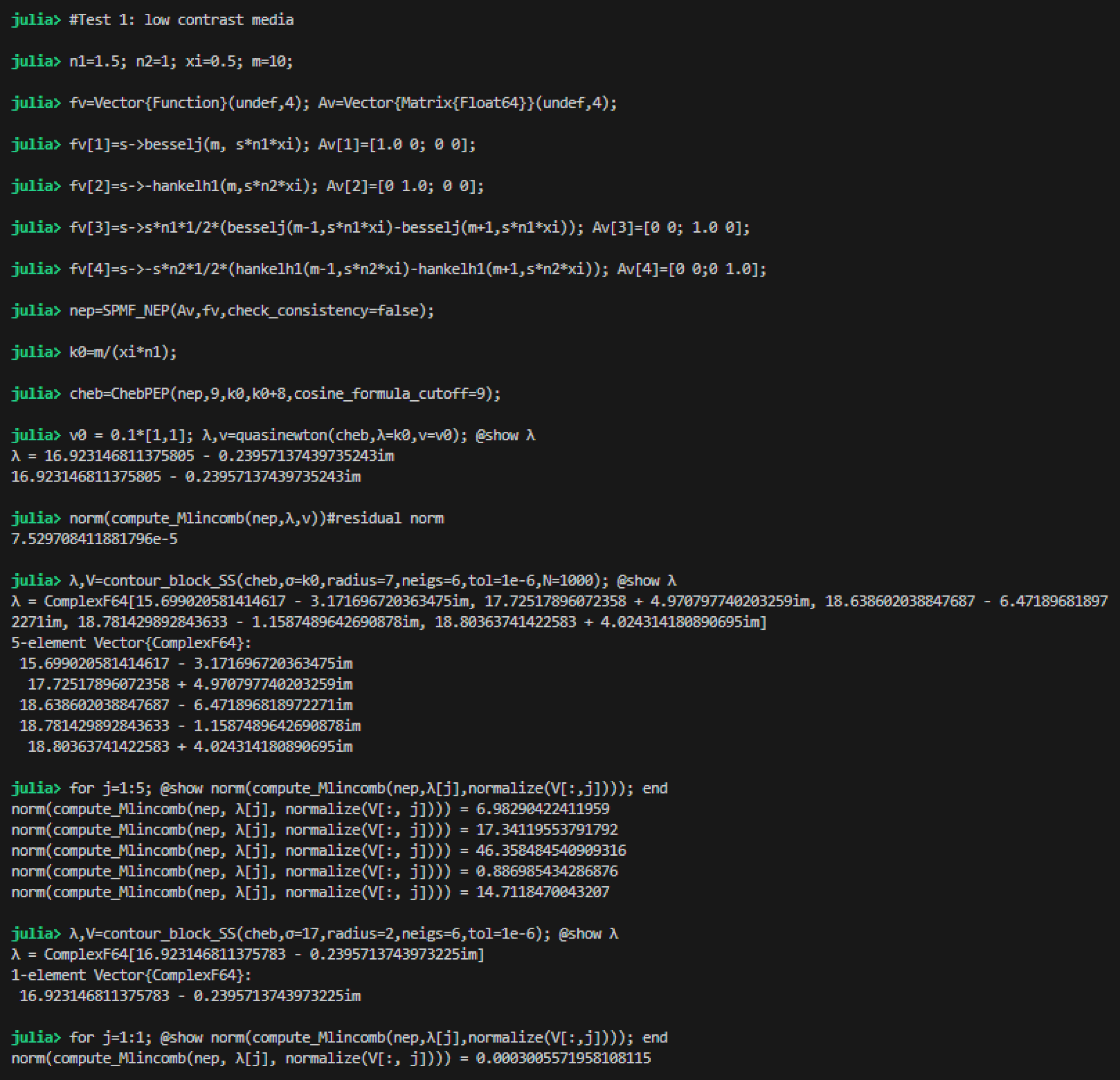
Figure S-1: Low-contrast media. Tests in the piecewise constant case using NEP-Package: comparison between Quasi-Newton method and Contour integral method, for $n_{1}=1.5$, $n_{2}=1$, $\xi=0.5$ and $m=10$.

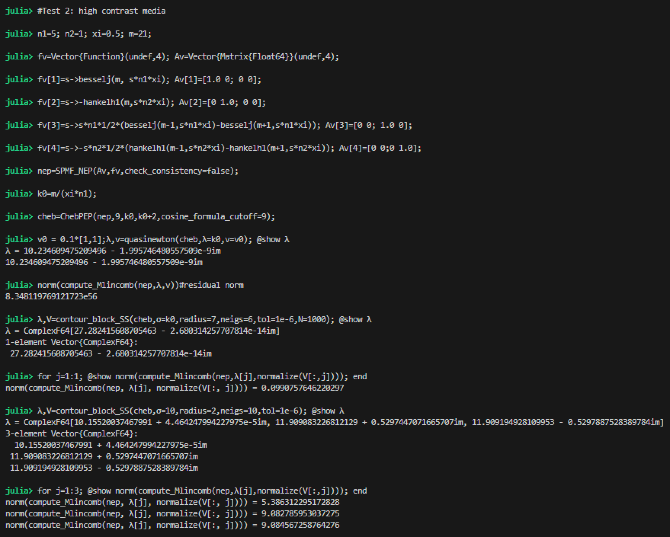
Figure S-2: High-contrast media. Tests in the piecewise constant case using NEP-Package: comparison between Quasi-Newton method and Contour integral method, for $n_{1}=5$, $n_{2}=1$, $\xi=0.5$ and $m=21$.

References

- [1] M. Abramowitz and I. A. Stegun. Handbook of mathematical functions with formulas, graphs, and mathematical tables, volume 55. US Government printing office, 1968.
- [2] G. Alessandrini. Strong unique continuation for general elliptic equations in 2D. J. Math. Anal. Appl., 386(2):669–676, 2012.
- [3] D. S. Alexander, F. Iavernaro, A. Rosa, et al. Early days in complex dynamics: a history of complex dynamics in one variable during 1906-1942. American Mathematical Society Providence, RI, USA, 2012.
- [4] C. Alves, A. Karageorghis, V. Leitão, and S. Valtchev. Advances in Trefftz methods and their applications. Springer, 2020.
- [5] C. J. Alves and P. R. Antunes. Numerical determination of the resonance frequencies and eigenmodes using the MFS. In Computational Methods, pages 1385–1389. Springer, 2006.
- [6] C. J. Alves and P. R. Antunes. Wave scattering problems in exterior domains with the method of fundamental solutions. Numerische Mathematik, 156(2):375–394, 2024.
- [7] J. C. Araujo-Cabarcas and C. Engström. On spurious solutions in finite element approximations of resonances in open systems. Computers & Mathematics with Applications, 74(10):2385–2402, 2017.
- [8] J. C. Araujo-Cabarcas, C. Engström, and E. Jarlebring. Efficient resonance computations for Helmholtz problems based on a Dirichlet-to-Neumann map. Journal of Computational and Applied Mathematics, 330:177–192, 2018.
- [9] J. Asakura, T. Sakurai, H. Tadano, T. Ikegami, and K. Kimura. A numerical method for nonlinear eigenvalue problems using contour integrals. JSIAM Letters, 1:52–55, 2009.
- [10] S. Balac, M. Dauge, and Z. Moitier. Asymptotics for 2D whispering gallery modes in optical micro-disks with radially varying index. IMA Journal of Applied Mathematics, 86(6):1212–1265, 2021.
- [11] W.-J. Beyn. An integral method for solving nonlinear eigenvalue problems. Linear Algebra and its Applications, 436(10):3839–3863, 2012.
- [12] A. V. Boriskin and A. I. Nosich. Whispering-gallery and Luneburg-lens effects in a beam-fed circularly layered dielectric cylinder. IEEE transactions on antennas and propagation, 50(9):1245–1249, 2002.
- [13] W. E. Boyce and R. C. DiPrima. Elementary differential equations, volume 6. Wiley New York, 2012.
- [14] O. P. Bruno, M. A. Santana, and L. N. Trefethen. Evaluation of resonances via AAA rational approximation of randomly scalarized boundary integral resolvents. arXiv preprint arXiv:2405.19582, 2024.
- [15] M. Dauge, S. Balac, G. Caloz, and Z. Moitier. Whispering gallery modes and frequency combs: Two excursions in the world of photonic resonators. In Book of Abstracts, The 16th International Conference on Mathematical and Numerical Aspects of Wave Propagation (WAVES 2024). Edmond, 2024.
- [16] E. Daya and M. Potier-Ferry. A numerical method for nonlinear eigenvalue problems application to vibrations of viscoelastic structures. Computers & Structures, 79(5):533–541, 2001.
- [17] S. Degtyarev, V. Podlipnov, P. Verma, and S. Khonina. 3d simulation of silicon micro-ring resonator with comsol. In International Conference on Micro-and Nano-Electronics 2016, volume 10224, pages 398–402. SPIE, 2016.
- [18] W. Dörfler and S. A. Sauter. A posteriori error estimation for highly indefinite Helmholtz problems. Comput. Methods Appl. Math., 13(3):333–347, 2013.
- [19] B. R. Fabijonas, D. W. Lozier, and F. W. Olver. Computation of complex Airy functions and their zeros using asymptotics and the differential equation. ACM Transactions on Mathematical Software (TOMS), 30(4):471–490, 2004.
- [20] E. F. Franchimon, K. R. Hiremath, R. Stoffer, and M. Hammer. Interaction of whispering gallery modes in integrated optical microring or microdisk circuits: hybrid coupled mode theory model. JOSA B, 30(4):1048–1057, 2013.
- [21] I. G. Graham and S. A. Sauter. Stability and finite element error analysis for the Helmholtz equation with variable coefficients. Math. Comp., 89(321):105–138, 2020.
- [22] B. Gräßle and S. A. Sauter. Dirichlet-to-Neumann operator for the Helmholtz problems with general wavenumbers on the -sphere. Technical Report in preparation, University of Zurich, 2025.
- [23] S. Güttel, D. Kressner, and B. Vandereycken. Randomized sketching of nonlinear eigenvalue problems. SIAM Journal on Scientific Computing, 46(5):A3022–A3043, 2024.
- [24] S. Güttel and F. Tisseur. The nonlinear eigenvalue problem. Acta Numerica, 26:1–94, 2017.
- [25] S. Hagness, D. Rafizadeh, S. Ho, and A. Taflove. FDTD microcavity simulations: design and experimental realization of waveguide-coupled single-mode ring and whispering-gallery-mode disk resonators. Journal of lightwave technology, 15(11):2154–2165, 1997.
- [26] P. Heider. Computation of scattering resonances for dielectric resonators. Computers & Mathematics with Applications, 60(6):1620–1632, 2010.
- [27] R. Hiptmair, A. Moiola, and E. A. Spence. Spurious quasi-resonances in boundary integral equations for the Helmholtz transmission problem. SIAM Journal on Applied Mathematics, 82(4):1446–1469, 2022.
- [28] K. Hiremath, R. Stoffer, and M. Hammer. Modeling of circular integrated optical microresonators by 2-d frequency domain coupled mode theory. Optics communications, 257(2):277–297, 2006.
- [29] T. Hohage and L. Nannen. Hardy space infinite elements for scattering and resonance problems. SIAM Journal on Numerical Analysis, 47(2):972–996, 2009.
- [30] V. S. Ilchenko and A. B. Matsko. Optical resonators with whispering-gallery modes-part II: applications. IEEE Journal of selected topics in quantum electronics, 12(1):15–32, 2006.
- [31] E. Jarlebring. Convergence factors of Newton methods for nonlinear eigenvalue problems. Linear algebra and its applications, 436(10):3943–3953, 2012.
- [32] E. Jarlebring, M. Bennedich, G. Mele, E. Ringh, and P. Upadhyaya. NEP-PACK: A Julia package for nonlinear eigenproblems-v0. 2. arXiv preprint arXiv:1811.09592, 2018. https://github.com/nep-pack.
- [33] D. Jerison and C. E. Kenig. Unique continuation and absence of positive eigenvalues for Schrödinger operators. Ann. of Math. (2), 121(3):463–494, 1985.
- [34] S. Kim and J. Pasciak. The computation of resonances in open systems using a perfectly matched layer. Mathematics of Computation, 78(267):1375–1398, 2009.
- [35] D. Kressner. A block Newton method for nonlinear eigenvalue problems. Numerische Mathematik, 114:355–372, 2009.
- [36] J. A. Lock. Scattering of an electromagnetic plane wave by a Luneburg lens. I. Ray theory. JOSA A, 25(12):2971–2979, 2008.
- [37] J. A. Lock. Scattering of an electromagnetic plane wave by a Luneburg lens. II. Wave theory. JOSA A, 25(12):2980–2990, 2008.
- [38] J. A. Lock. Scattering of an electromagnetic plane wave by a Luneburg lens. III. Finely stratified sphere model. JOSA A, 25(12):2991–3000, 2008.
- [39] J. M. Melenk and S. A. Sauter. Convergence Analysis for Finite Element Discretizations of the Helmholtz equation with Dirichlet-to-Neumann boundary condition. Math. Comp, 79:1871–1914, 2010.
- [40] A. Moiola and E. A. Spence. Acoustic transmission problems: wavenumber-explicit bounds and resonance-free regions. Mathematical Models and Methods in Applied Sciences, 29(02):317–354, 2019.
- [41] Z. Moitier. Étude mathématique et numérique des résonances dans une micro-cavité optique. PhD thesis, Rennes 1, 2019.
- [42] L. Nannen, T. Hohage, A. Schädle, and J. Schöberl. Exact sequences of high order Hardy space infinite elements for exterior maxwell problems. SIAM Journal on Scientific Computing, 35(2):A1024–A1048, 2013.
- [43] A. Neumaier. Residual inverse iteration for the nonlinear eigenvalue problem. SIAM Journal on Numerical Analysis, 22(5):914–923, 1985.
- [44] F. Olver, A. O. Daalhuis, D. Lozier, B. Schneider, R. Boisvert, C. Clark, B. Miller, B. Saunders, H. Cohl, and M. McClain. NIST Digital Library of Mathematical Functions. Release 2016. http://dlmf.nist.gov/.
- [45] S. Olver, G. Goretkin, R. M. Slevinsky, A. Townsend, and other contributors. ApproxFun.jl. https://github.com/JuliaApproximation/ApproxFun.jl, 2013-2015.
- [46] S. Olver and A. Townsend. A fast and well-conditioned spectral method. SIAM Review, 55(3):462–489, 2013.
- [47] S. Olver and A. Townsend. A practical framework for infinite-dimensional linear algebra. In Proceedings of the 1st Workshop for High Performance Technical Computing in Dynamic Languages – HPTCDL ‘14. IEEE, 2014.
- [48] A. M. Ostrowski. Solution of equations in Euclidean and Banach spaces. Academic Press, New York, 1973.
- [49] M. Oxborrow. Traceable 2-d finite-element simulation of the whispering-gallery modes of axisymmetric electromagnetic resonators. IEEE Transactions on Microwave Theory and Techniques, 55(6):1209–1218, 2007.
- [50] O. Poisson. Étude numérique des pôles de résonance associés à la diffraction d’ondes acoustiques et élastiques par un obstacle en dimension 2. ESAIM: Mathematical Modelling and Numerical Analysis, 29(7):819–855, 1995.
- [51] J. D. Pryce. Numerical solution of Sturm-Liouville problems. Oxford University Press, 1993.
- [52] M. A. Santana, L. N. Trefethen, and O. P. Bruno. Computation of Cavity Resonances via AAA Rational Approximation of Randomly Scalarized Boundary Integral Resolvents. In Book of Abstracts, The 16th International Conference on Mathematical and Numerical Aspects of Wave Propagation (WAVES 2024). Edmond, 2024.
- [53] S. Sauter and C. Torres. The heterogeneous Helmholtz problem with spherical symmetry: Green’s operator and stability estimates. Asymptotic Analysis, 125(3-4):289–325, 2021.
- [54] K. Schreiber. Nonlinear eigenvalue problems: Newton-type methods and nonlinear Rayleigh functionals. PhD thesis, TU Berlin, Germany, 2008.
- [55] O. Steinbach and G. Unger. Combined boundary integral equations for acoustic scattering-resonance problems. Mathematical Methods in the Applied Sciences, 40(5):1516–1530, 2017.
- [56] C. Sturm. Mémoire sur les équations différentielles linéaires du second ordre. Springer, 2009.
- [57] A. Townsend and S. Olver. The automatic solution of partial differential equations using a global spectral method. Journal of Computational Physics, 299:106–123, 2015.
- [58] H. Voss. Nonlinear eigenvalue problems. Handbook of Linear Algebra, 164, 2013.
- [59] G. N. Watson. A Treatise on the Theory of Bessel Functions. Cambridge University Press, 1966.
- [60] E. T. Whittaker and G. N. Watson. A course of modern analysis: an introduction to the general theory of infinite processes and of analytic functions; with an account of the principal transcendental functions. University press, 1920.
- [61] J. H. Wilkinson. The algebraic eigenvalue problem. Oxford University Press, Inc., 1988.
- [62] C. Yang, J. C. Meza, and L.-W. Wang. A trust region direct constrained minimization algorithm for the Kohn–Sham equation. SIAM Journal on Scientific Computing, 29(5):1854–1875, 2007.