Collecting Particles in Confined Spaces by Active Filamentous Matter

Abstract

The potential of compliant and adaptable active matter for particle transport presents a promising avenue for the development of efficient, autonomous systems. However, achieving optimal task efficiency often depends on external control mechanisms, which can limit the autonomy of such systems. In this study, we draw inspiration from Tubifex tubifex and Lumbriculus variegatus, centimeter-sized worms that exhibit an extraordinary ability to aggregate dispersed particles within confined environments. By observing their natural behaviors, we identify a simple yet effective particle collection strategy driven by flexibility and activity. Using these biological insights, we develop larger-scale robotic systems and simulations that replicate the particle aggregation dynamics of living worms. Our results reveal that coupling between activity and flexibility governs the efficiency of particle clustering, and this principle applies universally across biological, robotic, and simulated filaments. These results allow us to offer new particle collection strategies by tuning the design elements like topology or bending stiffness of soft active filaments.

Introduction

Active, flexible filamentous materials are essential to a variety of biological and synthetic systems, where their capacity for self-organization, mechanical force generation, and adaptability drives critical functions such as locomotion, resource collection, and environmental restructuring. Examples span from microscopic systems—motor-driven cytoskeletal filaments [1, 2, 3, 4, 5, 6] and cilia [7, 8]—to macroscopic organisms, including flagella [9, 10, 11], worms [12, 13], and snakes [14]. Synthetic analogs such as self-propelled robots extend these concepts, utilizing flexibility and activity to adaptively explore their surroundings [15, 16, 17].

One striking manifestation of active material functionality is particle aggregation, a process observed in both natural and engineered systems. In freshwater ecosystems, oligochaetes like Tubifex tubifex and Lumbriculus variegatus (California blackworms) use coordinated motion and mucus secretions to aggregate dispersed particles [2], enabling nutrient cycling and habitat stabilization. Similarly, robotic systems exploit activity and flexibility to manipulate inert (i.e., passive) materials, mimicking these natural behaviors to perform tasks like debris management and targeted delivery [17]. These aggregation dynamics are governed by the interplay between filament flexibility, activity, and the environmental context; yet, the precise mechanisms remain elusive.

Beyond biological systems, active-passive mixtures provide a simplified yet insightful framework to explore aggregation phenomena from an active matter perspective. Active agents such as colloidal Janus particles and robotic systems impose stresses and collisions on passive components, giving rise to emergent behaviors like clustering [19], phase separation [20, 21], and laning [22]. These processes may influence nutrient flows, structural formation, and ecosystem dynamics in natural habitats [23] while inspiring novel applications in material assembly and robotics [17]. Notably, the role of filament flexibility in such mixtures remains underexplored [24, 25], despite its relevance to both biological polymers [26] and synthetic systems [27, 17].

In this study, we bridge the gap between biological and synthetic active systems by investigating the particle collection dynamics of Tubifex tubifex and Lumbriculus variegatus in a controlled environment. We quantify the impact of their conformation and dynamics on particle aggregation efficiency. Extending these insights, we construct larger-scale robotic filaments and perform simulations to examine how variations in filament flexibility and length influence performance across biological, robotic, and simulated systems. Our findings suggest that flexibility and activity are central to enhancing particle collection efficiency, offering a robust framework for designing adaptable, soft robotic systems that can autonomously manipulate materials in constrained or complex environments.

Figure 1: Collection of passive particles by living, in silico, and robotic active filaments. (A) A California blackworm (Lumbriculus variegatus) in a petri dish with sand particles. Over time, the worm gathers the sand into larger clusters, eventually reaching a steady state, as shown by the evolution of the cluster size distribution over time in the final panel. Time is nondimensionalized by the characteristic time of one full passage of the filament’s center-of-mass across the cavity, $t^{*}\approx 120s$, allowing direct comparison across systems. (B) An active, tangentially driven filament interacting with passive crowders exhibits similar clustering behavior, where the cluster size distribution grows over time until reaching a steady state. (C) A robotic filament composed of connected Hexbug robots moves within a circular arena, interacting with passive styrofoam cubes. The robotic filament collects particles into clusters, ultimately reaching a steady state. $t^{*}\approx 5s$ (D) Design details of the robotic filament and a close-up view of the styrofoam particles. The robotic units are connected via elastic rubber bands of tunable width $\delta$, allowing control over the filament’s persistence length ($\ell_{p}/\ell_{c}$) and contour length ($\ell_{c}/D$).

Collecting Experiments

The particle collection ability of worms in confined environments presents both a biological puzzle and an exciting potential application for tasks such as microplastics collection, sorting, and cleaning [2]. To explore how this natural behavior can be generalized to active filaments, we investigated the collecting dynamics in three distinct active filament systems: two living centimeter-scale biological worms, T. tubifex and L. variegatus, which differ in aspect ratio; a meter-scale robotic filament, designed to isolate the effects of filament parameters such as elasticity and length; and Brownian dynamics simulation of an active filament with tangentially propelling force [28, 29, 30] to validate and extend our experimental observations. Despite the fact that these two worms have similar appearances and quantitatively comparable collective behaviors [12, 31], they exhibit distinct locomotion- diffusion-dominated random walks in T. tubifex and ballistic motion in L. variegatus—providing a unique opportunity to study and compare their mechanisms of dispersed passive particle collection [12].

Living biological filamentous worms. In our first quasi-2D experimental setup, we immersed a single Tubifex tubifex (with a typical length $L_{c}=4$ cm) and Lumbriculus variegatus ($L_{c}=3$ cm) into a 35 mm diameter Petri dish filled with thermostated water ($T=21^{\circ}$C) and $N_{\text{tot}}$ randomly dispersed $\sim$120 millimeter-scale pool filter sand particles ($d_{p,sand}=0.7$ mm, weight 50 mg). The particles are light enough so that inertia does not influence their dynamics.

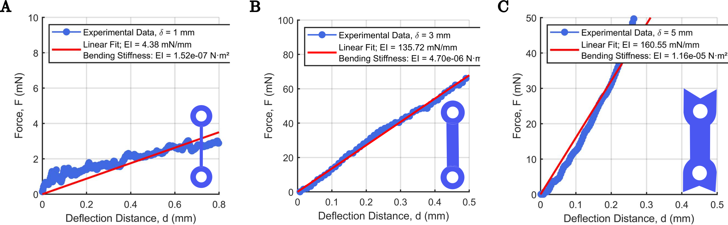
Figure S2: Bending stiffness of all elastic bonds used to tune the robotic filaments’ flexibility. The bending stiffness is measured with a rheometer by imposing the deflection of the elastic bond and measuring the force for three different widths: (A) $\delta$ = 1 mm; (B) $\delta$ = 3 mm; (C) $\delta$ = 5 mm.

When placed in the Petri dish, the worms, denser than water, crawl along the bottom via wiggling motion. Unlike algae or microplastics, which adhere to the worm’s mucus [2], sand particles do not stick to the body of the worm. Instead, the self-propulsion of the worm displaces the sand particles upon contact, which would otherwise remain stationary. This displacement occurs solely through direct interactions, as the worm’s motion does not generate significant fluid flow in the medium. Through repeated contact and passages in the dish -via reorientation of its direction at the boundary (Sup. Fig. S2), the worms actively gather particles into progressively larger clusters over time, as shown in Fig. 1A. However, the continuous energy input from the worm also fragments these clusters, preventing unrestricted growth and maintaining a quasi-steady state where clusters are constantly forming and breaking. Our findings suggest that this clustering behavior arises from the interplay between flexibility and dynamic adaptability of the active agent, revealing a mechanism distinct from the phase separation classically observed in dense active-passive mixtures [20, 19].

Using image analysis (Sup. Mat. Sec. I.C), we tracked the conformational dynamics of the worms and the positions of the particles, allowing us to characterize the distribution of cluster sizes over time. We define a group of $s$ particles as a cluster of size $s$, where each particle is within a distance of one particle size $d_{p,sand}$ from at least one other particle in the group. A typical result of the cluster size distribution $P(s)$ is shown in Fig. 1A, right. We find, as in previous works [32], that a power law combined with an exponential cut-off $P(s)=s^{-\gamma}\exp{(-s/s^{*})}$ gives a satisfactory description of our data, and yields an exponent $\gamma$ that increases in time (see Sup. Mat. Sec. III.D). Within a characteristic timescale of approximately 30 minutes, the cluster size distribution reaches a steady state. The average cluster size, $\langle s\rangle=\sum sP(s)$, at long times is typically $\langle s\rangle_{L}\approx$ 10 particles for both species of worms.

Figure 2: Effect of filament length and flexibility on collecting dynamics and long-time average cluster size. (A) Active filamentous systems are characterized by their flexibility ($\ell_{p}$) and contour length ($\ell_{c}$). (B) Larger cluster formation results from successive fragmentation and aggregation processes, driven by interactions between the particles and the active filaments’ conformations as they move through the cavity. (C) Effect of the active filament’s normalized stiffness ($\ell_{p}/\ell_{c}$) on the average cluster size. For all systems, the average cluster size grows over time before reaching a steady-state value $\langle s\rangle_{L}$ at long timescales, following Eq. 1. Higher filament stiffness leads to larger final cluster sizes. (D) For a fixed flexibility, the steady-state average cluster size increases with the normalized filament length ($\ell_{c}/D$). (E, F) Panels (C) and (D) include fits to Eq. 1, used to determine both the long-time steady-state cluster size $\langle s\rangle_{L}$ and the characteristic timescale $\tau=k_{\text{eff}}^{-1}$ for reaching steady state, as a function of filament stiffness ($\ell_{p}/\ell_{c}$).

Figure 3: Evolution of the cluster’s average location over time. (A) Sequence of images ($t/t^{*}$ = 0; 52; 120) showing the spatial evolution of particle positions over time. (B) Average radial position of the cluster as a function of time for the three different active filamentous systems. Long filaments ($\ell_{c}/D\sim 1$) tend to accumulate at the center of the cavity compared to short ones ($\ell_{c}/D\sim 0.3$), while their stiffness has minimal influence on their final position.

Active polymer simulation. We perform Brownian dynamics simulations using an active polymer model [28, 29, 33] (see Sup. Mat. Sec. II.A for details on the numerical methods and model), which has been shown to effectively capture the behavior of these worms [34]. Each monomer in the polymer follows overdamped Langevin dynamics, driven by an active force of amplitude $f^{a}$ applied tangentially along the filament backbone. The flexibility of the active polymer is controlled by the bending stiffness $\kappa$ between neighboring bonds. (Fig. 1B). In addition to the polymer length, the key parameters in our model are therefore reduced to $f^{a}$ and $\kappa$. Passive particles, which are half the size of monomer $\sigma$ ($d_{p,sim}=0.5\sigma$), are initially placed in a homogeneous concentration throughout the simulation domain. The experiments involving sand particles and worms reveal that there is no adhesion between them and that there is no fluid flow generated by the worm to displace the sand particles, suggesting short-range steric interactions between the active polymer and passive particles. Consequently, the passive particles remain stationary until pushed by active polymer segments and interact repulsively with each other and with other particles only within their respective cutoff distances. Thus, our model describes a dry active system in which the medium contributes only single-particle friction and does not include hydrodynamic interactions.

To ensure realistic boundary conditions, we place stationary particles along the circumference of a circular boundary of radius, $R$ = 25 $\sigma$. These boundary particles impart a steric-like repulsion to the active polymer and passive particles. Additionally, three-bead triangular re-injectors are positioned along the circular boundary at regular angular intervals $30\degree\theta$, with their apexes pointing toward the center of the confining circle.

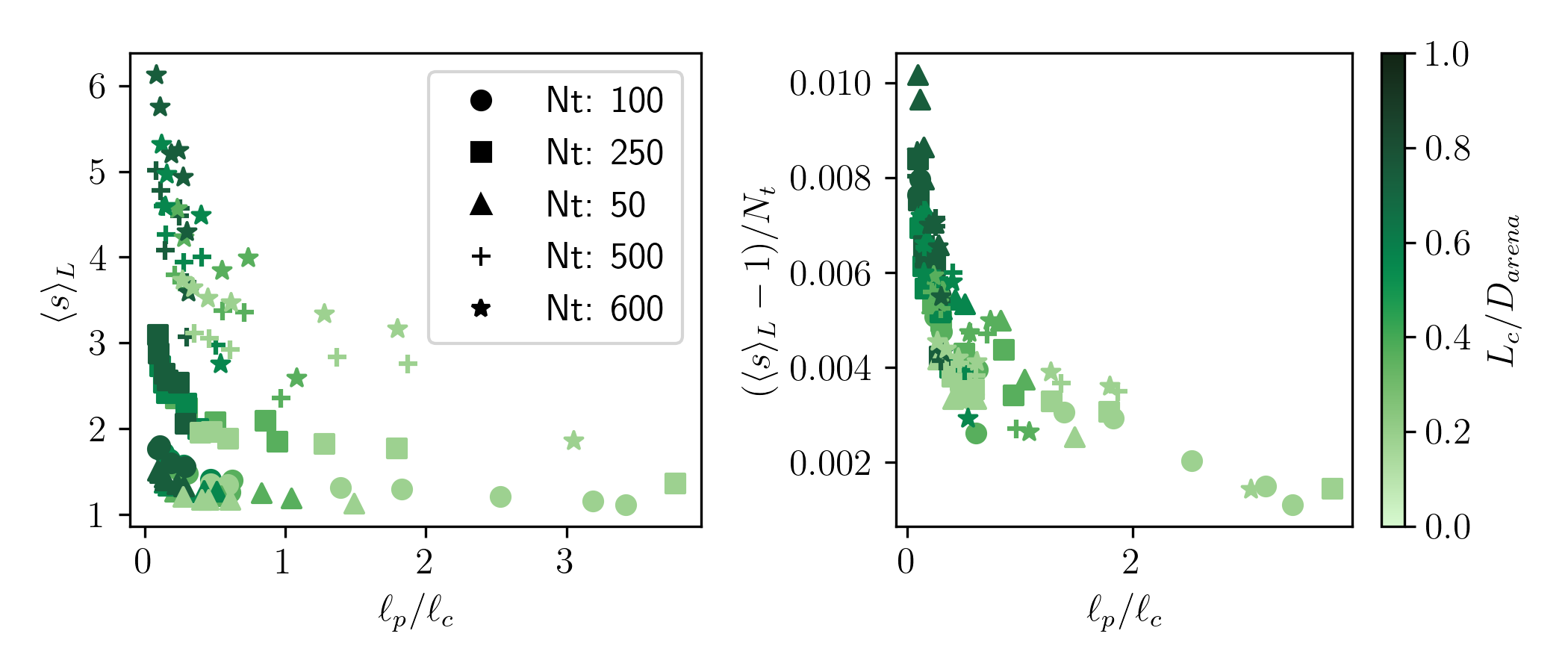
Figure S8: Effect of initial particle density on the long-time average cluster size. (Left) The long-time average cluster size from simulations is plotted as a function of the normalized persistence length $\ell_{p}/\ell_{c}$. We examined densities ranging from 50 to 600 passive particles. (Right) Same data as in (Left), but rescaled as $(\langle s\rangle_{L}-1)/N_{t}$, allowing collapse of all the data on the same curve.

This approach, commonly used in persistent active systems, prevents the filament from getting trapped along the walls [35, 36]. When gliding near the wall, the tangentially driven filament is reoriented into the bulk of the arena by these triangular re-injectors, closely mimicking the behavior observed in biological worms (see Sup. Fig. S2). We find that the exact spacing of the re-injectors has no significant effect on the cluster formation. (see Sup. Fig. S8)

We find that the dynamics of the simulated active filament closely resemble those of the living worms, and the particles aggregate into clusters over time in a similar fashion (see the sequence of pictures in Fig. 1B). This is confirmed by the cluster size distribution, which exhibits the same power-law behavior as in the worm experiments, with the distribution shifting toward larger values as time progresses (Fig. 1B, right).

Robotic filament. In our second experimental setup, we scaled up the worm experimental platform to the meter scale and transformed it into a robotic filament enclosed within a fixed arena of meter diameter (Fig. 1C). Our active filament is composed of $N$ commercially available self-propelled microbots (Hexbug Nano v2 with a characteristic size, $\sigma_{unit}$ = 45 mm) [37, 27, 38, 16, 17], encased in a 3D-printed frame around each individual bot and elastically coupled by laser-cut silicone rubber connectors (Fig. 1C; see also Sup. Mat. Sec. I.B). Adjusting the width of the connections ($\delta$ in the close-up of the Fig. 1C), we can fine-tune the stiffness of the filament, $\kappa$. When constrained at zero velocity, each bot exerts an active force $f^{a}\sim 15~mN$ in the direction of its polarization, tangential to the filament’s axis[16].

To enclose the robotic filament, we used a rigid metal circular boundary with a 120 cm diameter. To maintain consistency with our simulations, we incorporated defects at the boundary to re-inject the robotic filament into the bulk of the arena. The initially dispersed $N_{tot}=120$ passive cubic particles, made of lightweight styrofoam, ensure that their weight does not play a role in the dynamics of the active robotic filament.

Interestingly, we observe that the robotic filament interacts with the particles in a manner similar to the biological and simulated systems, as confirmed by the probability distribution of cluster sizes over time. This raises the question of why and how these active filaments, seemingly displaying universal behavior, manage to collect particles when confined in a circular arena. To address this, we investigate the underlying factors that govern this particle collection process.

Dynamics of aggregation & spatial distribution

Aggregation-fragmentation dynamics. To investigate the mechanisms driving particle clustering across our different active filament systems, we tracked the aggregation dynamics by measuring the average cluster size, $\langle s\rangle$, over time. We also examined the influence of two key filament parameters: contour length ($\ell_{c}$) and stiffness (Fig. 2A). In the robotic system, $\kappa$ is controlled by adjusting the width of the elastic bonds ($\delta$), with larger $\delta$ corresponding to increased stiffness, while in the simulations, $\kappa$ is tuned directly. From the sequence of images, we measured the effective persistence length ($\ell_{p}$) of the filaments, which correlates with the initial stiffness $\kappa$, but also accounts for the change in its conformation with activity and its interactions with the boundary, where the filaments tend to curl while following the edge of the arena.

In all three experiments, the passive particles are initially randomly distributed, and an active filament is subsequently introduced in every system. As time progresses, we observe that the active filaments swipe particles along their paths, inducing both particle aggregation and dissociation (Fig. 2B). This process leads to the formation of larger clusters over time, akin to an aggregation-fragmentation mechanism, similar to polymerization reactions [39, 40]. After a transient period, the system reaches a steady state where the average cluster size stabilizes, indicating a balance between aggregation and fragmentation. In this analogy, the active filament acts as a dynamic reactor, driving both the aggregation and fragmentation of particle clusters. As shown in Fig. 2C, in all cases, the average number of particles in a cluster, $\langle s\rangle$, follows a logistic growth model, eventually reaching a long-term steady-state average cluster size, $\langle s\rangle_{L}$. The growth process is accompanied by fluctuations, which are signatures of cluster breakup (i.e, fragmentation), as the active filament dissociates the clusters. The average cluster size growth stabilizes over a characteristic timescale, $\tau={k_{\text{eff}}}^{-1}$.

We find that the evolution of the average cluster size across all systems follows a saturating exponential behavior (Figs. 2C,D), which is well described by the expression:

$$\langle s(t)\rangle=1+\langle s\rangle_{L}\left(1-e^{-k_{\text{eff}}t}\right).$$ (1)

This functional form suggests an underlying aggregation-fragmentation process, where clusters grow and break apart at effective rates $k_{a}$ and $k_{f}$, leading to a characteristic timescale $\tau=1/k_{\text{eff}}$. To model this behavior, we treat the system as a binary process, where aggregates of any size $s_{n}$ undergo aggregation ($k_{a}$) and fragmentation ($k_{f}$) at the same rates, independent of size:

$$[s_{1}]+[s_{2}]\underset{k_{f}}{\stackrel{{\scriptstyle k_{a}}}{{\rightleftharpoons}}}[s_{1}+s_{2}].$$

By fitting our data to Eq. 1, we extract both the long-term average cluster size, $\langle s\rangle_{L}$, and the effective growth rate, $k_{\text{eff}}=k_{a}+k_{f}$, which determines the timescale for the system to reach steady state. Notably, we find that this characteristic timescale $\tau$ is nearly independent of filament length and stiffness across different active filament systems (Fig. 2E). The system reaches steady state after approximately $\tau/t^{*}\approx 35$ sweeps, where $t^{*}$ is the typical time for a filament to cross the circular confinement (Worms: $t^{*}\approx 120s$, Robots: $t^{*}\approx 5s$).

Interestingly, the final cluster size $\langle s\rangle_{L}$ is influenced by both the flexibility and the contour length of the active filaments. As shown in Figs. 2C,D, the normalized flexibility ($\ell_{p}/\ell_{c}$) and the ratio of filament contour length to system size ($\ell_{c}/D$) both affect the long-term cluster size: longer and more flexible filaments tend to form larger clusters. Furthermore, Fig. 2F indicates that the ratio of persistence length to contour length ($\ell_{p}/\ell_{c}$) captures a general trend: More flexible filaments (i.e, lower $\ell_{p}/\ell_{c}$) tend to produce larger average clusters. However, this trend does not lead to a universal collapse across the diverse systems studied—biological, robotic, and simulated active filaments. This suggests that an additional parameter governs clustering dynamics more directly, which we explore in the next section.

Spatial distribution. We also examine the final location of clusters within the enclosed circular arena. In Fig. 3(A), we present a typical sequence of images that illustrate the clustering of particles toward the center of the cavity. The average radial position is $r=0$ when all particles are fully centralized, while for an initially random distribution, it is $r=2/3$.

As shown in Fig. 3, long and flexible active filaments tend to aggregate particles toward the center of the cavity across all the active filamenteous system studied here. In contrast, shorter filaments ($\ell_{c}/D\lesssim 0.3$) and stiffer filaments ($\ell_{p}/\ell_{c}\gtrsim 0.5$) exhibit a tendency to accumulate particles away from the center. In the limit of short filament length, this behavior resembles that of active point-like particles in a bath of passive particles, which tend to accumulate near the boundary or form a dispersed gas-like state [27, 41].

Active Swiping Collecting Mechanism

Figure 4: A simplified model for particle aggregation dynamics. (A) Simulation of an active filament sweeping through a field of particles, progressively clustering them into larger aggregates over time. (B) Heatmap of the filament’s trajectory (blue), showing the regions it has traversed. As the filament moves, it clears particles along its path of width $W$, leaving unvisited areas where particles accumulate. (C) To abstract this process, we model particle displacement using a simplified system where sticks of width $W$ (representing the filament) sweep particles at each timestep within a confined cavity. The sweeping bands are randomly placed and oriented either horizontally or vertically. (D) Steady-state cluster formation. The inset shows the evolution of the average cluster size over time, showing that the simplified model captures the aggregation dynamics observed in experiments and simulations [Fig. 2(C,D)].

A detailed analysis of the conformation of active filaments during exploration reveals that they actively sweep particles away from their path as they move through the arena. As shown in the sequence of snapshots obtained from the simulation in Fig. 4A, the trajectory of an active filament over time leaves behind a cleared path of effective width $W$. A probability density map of the filament’s center-of-mass position over the entire course of its motion further reveals that the filaments spend a significant portion of their time near the boundary, effectively pushing particles away from it.

As mentioned before, despite the influence of filament’s length and flexibility on clustering (Fig. 2F), this relationship does not lead to a universal collapse across our different systems we studied here. This suggests that another parameter governs the clustering dynamics more directly.

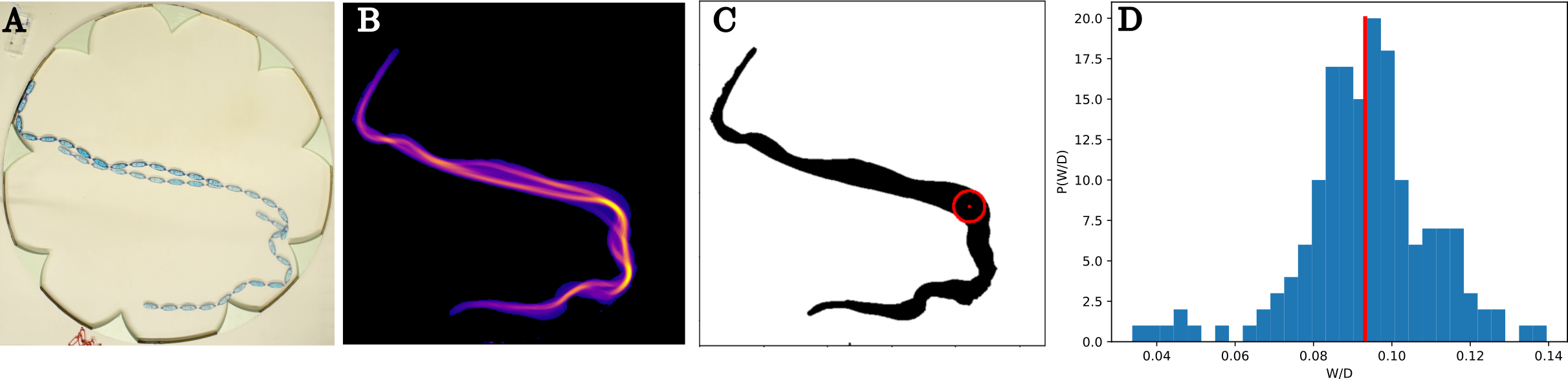
Figure S6: Method for measuring the sweeping width, $W$. (A) Superimposed images over a time interval equal to the typical crossing time $t^{*}$ of a filament (showing only the start, middle, and end frames for clarity). (B) Heatmap of the filament’s positions over the time window $t^{*}$. (C) Binary mask of the heatmap shown in (B), with the largest possible inscribed circle defining the sweeping width $w$ highlighted in red. (D) Distribution of measured $W$ values over an entire experiment for the filament shown in (A) (14 bots, 1 mm connector). The red line represents the median of this distribution.

Instead, we propose that the clustering process is better characterized by the effective footprint width, $W$, defined as the (average) transverse extent of the pathway cleared by the filament’s trajectory. As shown in Fig. 4A, $W$ depends on the filament’s flexibility and length, with longer and more flexible filaments generally generating wider pathways. To quantify $W$, we first superimpose all a filaments contours in the period of time it takes the filament to make one crossing, to find the filaments footprint. Next we fit the largest circle that can be inscribed inside this footprint, and take the diameter of this circle to be the footprint width (see Sup. Fig. S6). Systematic measurements (Sup. Fig. S9) confirm that more flexible filaments tend to exhibit greater transverse fluctuations relative to their tangential motion, leading to wider footprints. These fluctuations result from the complex conformation of the active polymer due to the interplay between filament activity, flexibility, and interactions with the arena boundaries.

Remarkably, when the final average cluster size $\langle s\rangle_{L}$ is plotted as a function of $W$ normalized by the system dimension $D$, all data from Fig. 2F collapse onto a single master curve, Fig. 5. This establishes $W$ as the key parameter governing the clustering process for values of $W/D\leqslant 1$: the larger the effective footprint width, the larger the final average cluster size. Since $W$ is set by filament flexibility and length, these properties indirectly dictate the clustering dynamics.

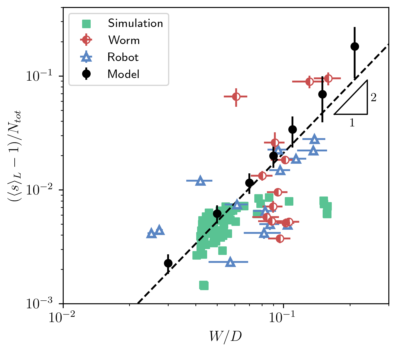
Figure 5: Steady-state cluster size as a function of the average active filament footprint width. The long-time average cluster size from all experiments and simulations collapses onto a single master curve, showing a quadratic dependence on the average footprint width $W$.

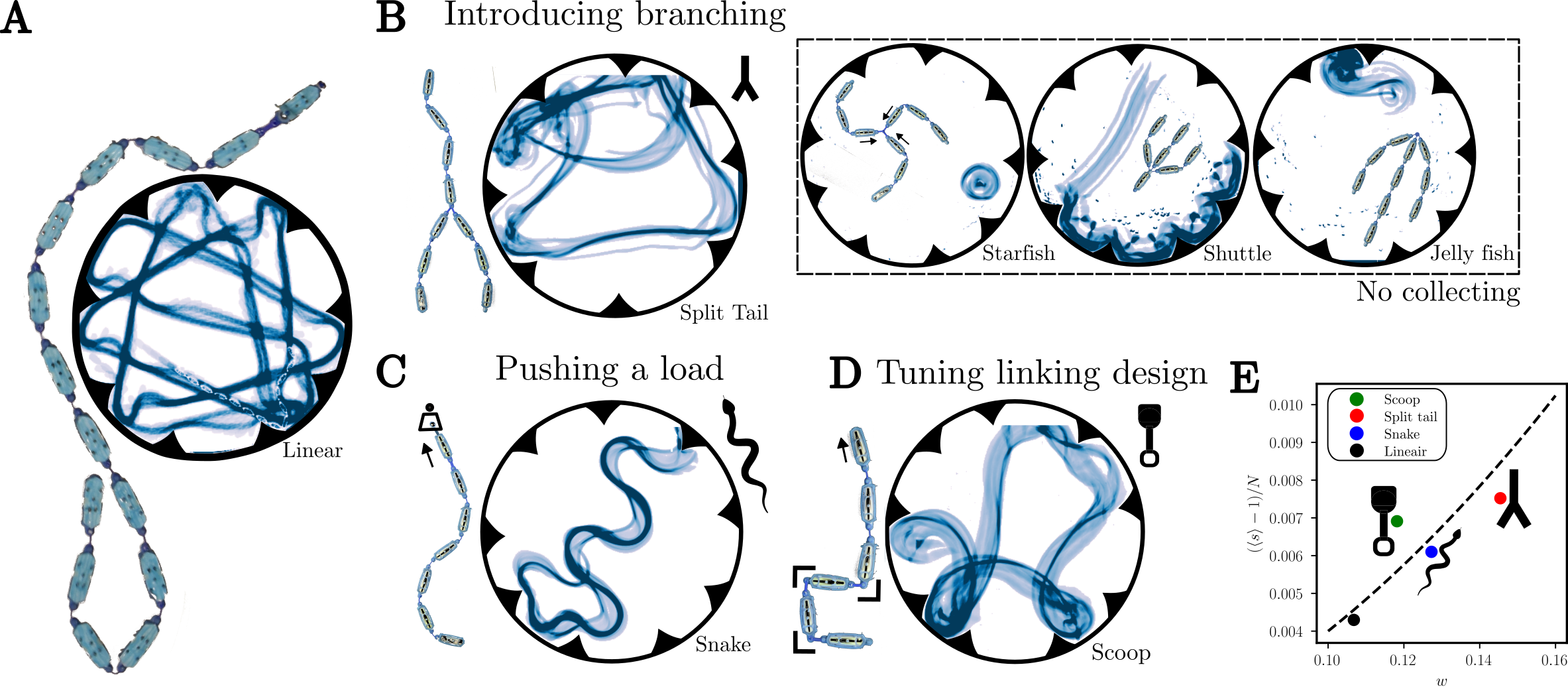
Figure 6: Active filament Atlas: A design space for optimizing particle collection through active filament chain properties. (A) Baseline linear polymer configuration. (B) A first strategy modifies chain topology by introducing branches, altering sweeping dynamics. Trajectories of each robotic unit within the chain illustrate distinct collection strategies. (C) A second strategy adjusts the speed of the leading bot by increasing its weight, inducing self-oscillatory motion along the path. (D) Tuning the elasticity of individual bonds enables the imposition of complex, pre-programmed curvatures during motion. (E) The resulting collection efficiencies, quantified by the long time average cluster size ($\langle s\rangle_{L}$), are compared to those of the linear chain. This active robotic filament at last establishes a taxonomy for emergent, multi-filament, heterogeneous flexible structures, paving new directions for engineering artificial active materials with programmable shape adaptation and collective functionality.

To understand the scaling behavior of $\langle s\rangle_{L}$ with $W$ observed in Fig. 5, we propose a minimal computational model. In this model, we start with a box of size $L\times L$ with $N_{t}$ passive particles. Clustering occurs as particles are swept away from a region of size $L\times W$, representing the effective path cleared by the active filaments (see Fig. 4C). Initially, the particles are uniformly distributed throughout the arena. Over time, repeated filament sweeps along both axes push particles away from these regions, leading to two competing effects: Aggregation—Particles accumulate into larger clusters as they are displaced from swept regions, and Fragmentation—Clusters can be disrupted when the filament path crosses an aggregate.

This minimal model quantitatively reproduces the experimentally observed clustering dynamics, as confirmed in the inset of Fig. 4D, where the predicted cluster growth dynamics align with the experimental and simulation data of Fig. 2C,D. Additionally, the time scale to reach a steady state also aligns very well with our experimental findings: after $\sim$ 35 iterative sweeps, we converge to the steady state (see the supplementary material for more details on the results of these simulations.)

The aggregation and fragmentation of particle clusters can be described by the Smoluchowski aggregation equation [8, 39], which applies to irreversible aggregation and thus has inherent limitations in the context considered here (Sup. Mat. Sec. III.B). This theory relies on a mean-field approximation, assuming that each cluster interacts equally with all others, regardless of their relative separation. However, this assumption breaks down in our system, where the aggregation and fragmentation processes are governed by the motion of the active polymer, which introduces spatial correlations and disrupts the equivalence between clusters. Instead, we provide a scaling argument to capture the underlying dynamics.

Let $a$ be the typical distance between two clusters and $R$ the typical cluster size. If the cluster size distribution is sufficiently narrow, meaning clusters are approximately the same size, then $a\sim R$. At steady state, clusters remain unaffected by the sweeping process when separated by a distance on the order of $w$, giving $a\sim w$. Combining these two conditions, we obtain $R\sim w$. Since the number of particles per cluster scales as $R^{2}$, this immediately leads to the scaling law $\langle s\rangle_{l}\sim w^{2}$, which rationalizes the experimental and simulation data collapse shown in Fig. 5.

As shown in Fig. 5, our simulations (black dots) and scaling argument (continuous line) predict that the long-time average cluster size scales as $W^{2}$, closely matching experimental results. This good agreement between theory, simulations, and experiments confirms that the effective swiping width $W$ is the key parameter governing the clustering process.

Discussion

Tubifex tubifex and Lumbriculus variegatus worms occupy a region of large final average cluster size (Fig. 5), indicating that their particle aggregation strategies are mechanically optimized. However, our active swiping model predicts a broader parameter space of particle collection strategies, within which these biological systems operate in a narrow, efficient regime. For instance, filaments with higher flexibility demonstrate increased footprint width $W$, enhancing their ability to collect particles. This relationship underscores the importance of flexibility in facilitating robust particle aggregation, yet highlights the diversity of potential behaviors beyond the biological systems observed here.

While our experiments demonstrate that flexibility and activity drive efficient clustering in biological filaments, this principle extends to synthetic systems. Our robotic filaments, designed with tunable flexibility, replicate the swiping and collecting efficiency observed in worms. The ability to adjust the effective footprint width, $W$, provides a strategy for optimizing particle collection across various scales, underscoring the role of mechanical adaptability in enhancing performance. Several strategies can be employed to improve the collection efficiency of an active filament, as illustrated in Fig. 6. One approach involves modifying the topology of the active chain by introducing branching structures (Fig. 6B). Another strategy consists of tuning the weight distribution of the leading bots in the robotic chain, causing them to move more slowly than the rest. This introduces a non-homogeneous active force along the chain, inducing dynamic oscillations that effectively increase its interaction width (Fig. 6C). As a result, the robotic chain can potentially enhance particle collection with tunable kinetics, as shown in Fig. 6D. In these cases, the long-time average cluster size, $\langle s\rangle_{L}$, improves compared to the linear chain of bots as $W$ increases. There are some limits to this design space however; whenever filaments get too wide, by for example introducing branching at the front of the filament or using monomers of increased size, the filaments get irrevocably stuck at the boundaries. This observation points to another way the worms are very well optimized for their environment. Considering that the footprint width is a dynamic quantity stemming from the transverse fluctuations of the worm, a polymer-like shape allows the worm to adapt to its environment effectively, becoming narrow where needed and wide where possible.

The generality of these findings opens up multiple avenues for future research. By manipulating filament flexibility and activity, it may be possible to program active filaments for tasks such as self-organized material assembly or environmental manipulation without the need of external control and feedback. Although our study highlights that active filaments hold immense promise for developing innovative methods to assemble passive objects, achieving effective control remains a significant challenge, hindering their full realization in practical applications. For instance, in applications involving the targeted transport of passive particles by the active filament, precise control of their trajectory is difficult due to the randomness in the motion of active filament. Designing methods for automated control of passive particle assembly, such as creating predefined pathways/footprints for the active filament motion or guiding the motion of active filaments through controlled interactions, represents a promising avenue that remains largely unexplored. Moreover, extending this framework to systems of packed or tangled filaments could uncover new topological states or behaviors, enriching our understanding of how active materials function across scales.

In summary, our study establishes that flexibility and activity play a central role in emergent behaviors such as efficient particle collection, providing a unified framework that connects biological, robotic, and simulated active filaments. The principles uncovered here open promising avenues for the design of soft, adaptive robotic systems and multifunctional active materials, with applications spanning various length scales—from environmental remediation to autonomous fabrication.

Supplementary Materials for
“Collecting Particles in Confined Spaces by Active Filamentous Matter’

This Supplementary Material provides additional information on the different active filamentous systems investigated, the experimental setup, and methodologies employed in this study, and on the polymer model and simulation details used for our analysis.

I EXPERIMENTS

I.1 Living Worms

We investigated particle collection using two different species of annelid worms. These species are widely available from commercial supplies and differ in their aspect ratio, persistence length, and motility dynamics, providing a valuable basis for comparison.

I.1.1 Californian blackworms

We purchased California blackworms (Lumbriculus variegatus) from Ward’s Science and were reared similarly as described in past publications ([1, 2, 3]).

I.1.2 Tubifex Tubifex worms

A second species of living worms that we studied was Tubifex tubifex, a living biological system that has been previously investigated in other recent studies [4, 5, 6, 7]. All batches of T. tubifex worms analyzed in this work were purchased from the provider Aquadip (https://www.aquadip.nl/) and ordered in a prepacked configuration, where the worms were at adult size. Their contour length $\ell_{c}$ vary between 20 and 40 mm and their width is typically 0.8 mm. The worms were maintained in an aquarium at room temperature, constantly under filtered flow, with water consisting of demineralized water mixed with salt solutions optimized for their needs. The salt solution consist of a mixture of: 50 g/L of NaHCO3; 10 g/L of KHCO3; 100 g/L of CaCl2; 90 g/L of MgSO4. Worms were fed weekly with standard goldfish food, and the water was refreshed once per week or more frequently if needed.

I.1.3 Experimental setup

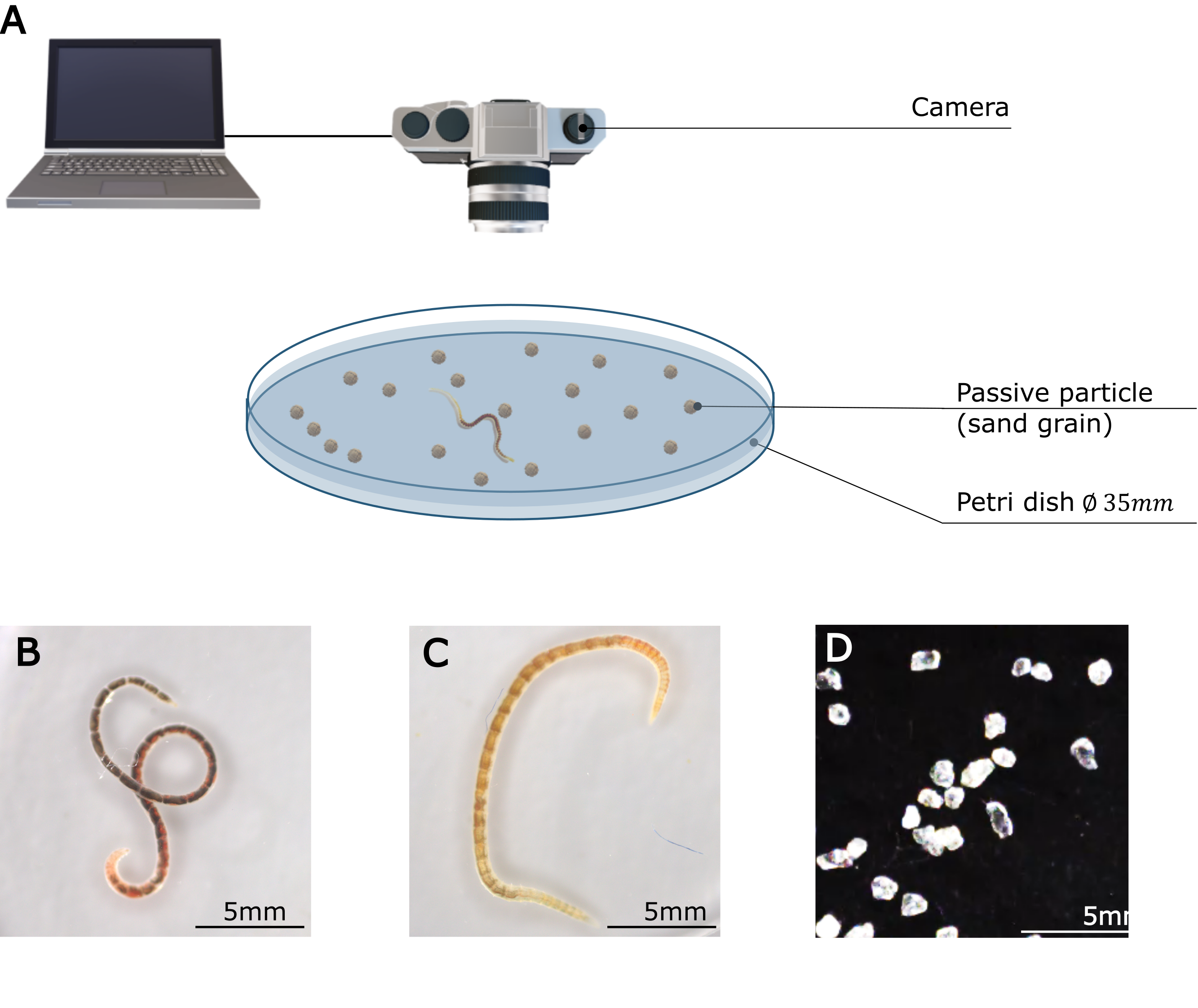
Figure S1: Experimental setup for investigating particle collection by worms. (A) A 35 mm diameter petri dish is filled with fresh water and $50$ mg of sand particles with a typical size of 1 mm. (B) A T. tubifex worm or (C) A California blackworm is introduced into the dish to study particle collection. (D) Snapshot of the sand particles used in the experiments.

To investigate particle collection by worms, we mounted an ImageSource DFK 33UX264 camera (Charlotte, NC) on an optical table using 80/20 parts. The experimental protocol is described similarly in Tuazon, et al. [2]. We recorded each experiment at a frame rate of 20 FPS for four hours with fixed lighting, where the first three hours were used for data analysis. 50$\pm$0.01 mg of 20# palmetto pool filtered sand (Woodruff, SC) were used for the test materials where $\sim$0.7 mm grains were isolated using nylon mesh. The sand grains were transferred in a 35 mm Petri Dish and submerged in 2 mm of filtered water. Before worm transfer, the sand grains were manually dispersed using a pipet (to ensure that the grains were evenly distributed).

After undergoing a one hour habituation period, worms were transferred in the Petri Dish with the sand grains. We repeated this experiment 11 times for blackworms and 3 times for T.tubifex.

I.2 Robotic filament

As mentioned in the main text, the robots that are at the basis of our robotic filaments are commercially available bristle bots “Hexbug”, the Hexbug Nano Nitro. (https://www.hexbug.com/) Bristle bots are a class of self-propelled robots that exhibit active Brownian motion. They consist out of a body housing some electronics supported by bristles. The bristle bots are able to locomote due to a battery powered off-balance flywheel that causes the robot to vibrate. This vibration causes the weight pressing on the bristles to fluctuate, propelling the bot in a random direction at each oscillation. The bristles underneath the Hexbug nano are slightly curved backward, which causes a bias in the direction the bot is propelled and allows the movement of the bot to be more persistently forward.

To construct our robotic filaments, individual Hexbug units were enclosed in a custom-designed 3D-printed housing. Each housing was equipped with small protrusions at the front and back, allowing for the attachment of flexible sillicone rubber connectors. These connectors, laser-cut to precise dimensions, served as elastic joints between adjacent robots, enabling controlled variations in the filament’s flexibility. A schematic representation of the housing and the experimental arena, along with relevant dimensions, is provided in Sup. Fig. SS4.

The bending stiffness of the rubber connectors was systematically tuned by adjusting their width, allowing us to investigate robotic filaments with a broad range of persistence lengths. By varying both the number of bots in the chain (contour length) and the stiffness of the connectors, we were able to explore the effects of filament flexibility on clustering dynamics. A summary of the effective persistence lengths and corresponding bending stiffness values for all tested configurations is provided in the Sup. Table 1 and Sup. Fig. SS2.

Across different persistence and contour lengths, we observed a variety of distinct motion patterns. Stiffer filaments exhibited more persistent trajectories, often skimming along the arena boundary, whereas more flexible filaments displayed increased curvature in their paths. Extremely long and highly flexible filaments occasionally became trapped in self-induced spirals. This effect was mitigated by reinforcing the frontal connector, reducing excessive bending at the leading end. Representative trajectories illustrating these behaviors are shown in Sup. Fig. SS3.

We note that individual bristle bots can exhibit a slight turning bias in their trajectories, despite careful preselection to mitigate this effect. This bias arises from minor asymmetries in their internal construction. While visible in recorded trajectories, its overall impact on clustering efficiency remains negligible.

I.2.1 Experimental setup and protocol

The experiments were conducted in an arena enclosed by a metal barrier, with re-injection defects positioned around the inside perimeter. One hundred styrofoam cubes (20 mm per side) were painted black to serve as passive particles. A camera was positioned above the arena to capture the experiment from a top view perspective (see Sup. Fig.S S4).

Before each experiment, the tracer particles were evenly distributed within the arena. The robotic filament was then turned on and carefully placed into the arena to minimize disturbance to the particles before the experiment commenced. The recording began immediately after the filament was introduced.

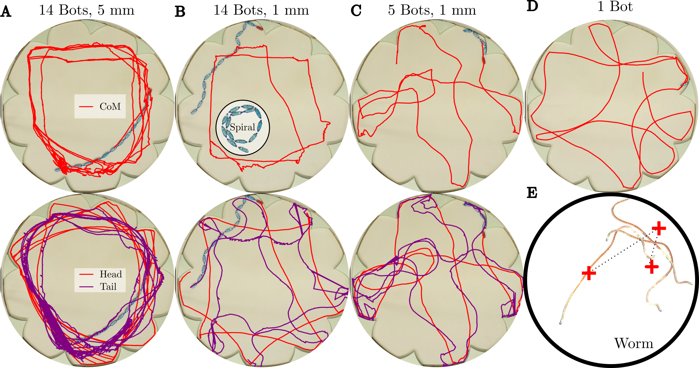
Figure S3: Trajectories of the head, tail, and center of mass for three representative robotic chains. (A) A long, stiff robotic chain predominantly follows the arena boundary, with the tail bot closely tracing the path of the leading bot. (B) A long, flexible robotic chain also remains near the boundary, but the tail bot exhibits pronounced undulations around the path of the leading bot. (C) A short robotic chain navigates more frequently through the center of the arena. (D) Center of mass trajectory of a single Hexbug (E) Superimposed images of a blackworm, showing how the worms deflects from the boundary of the petridish.

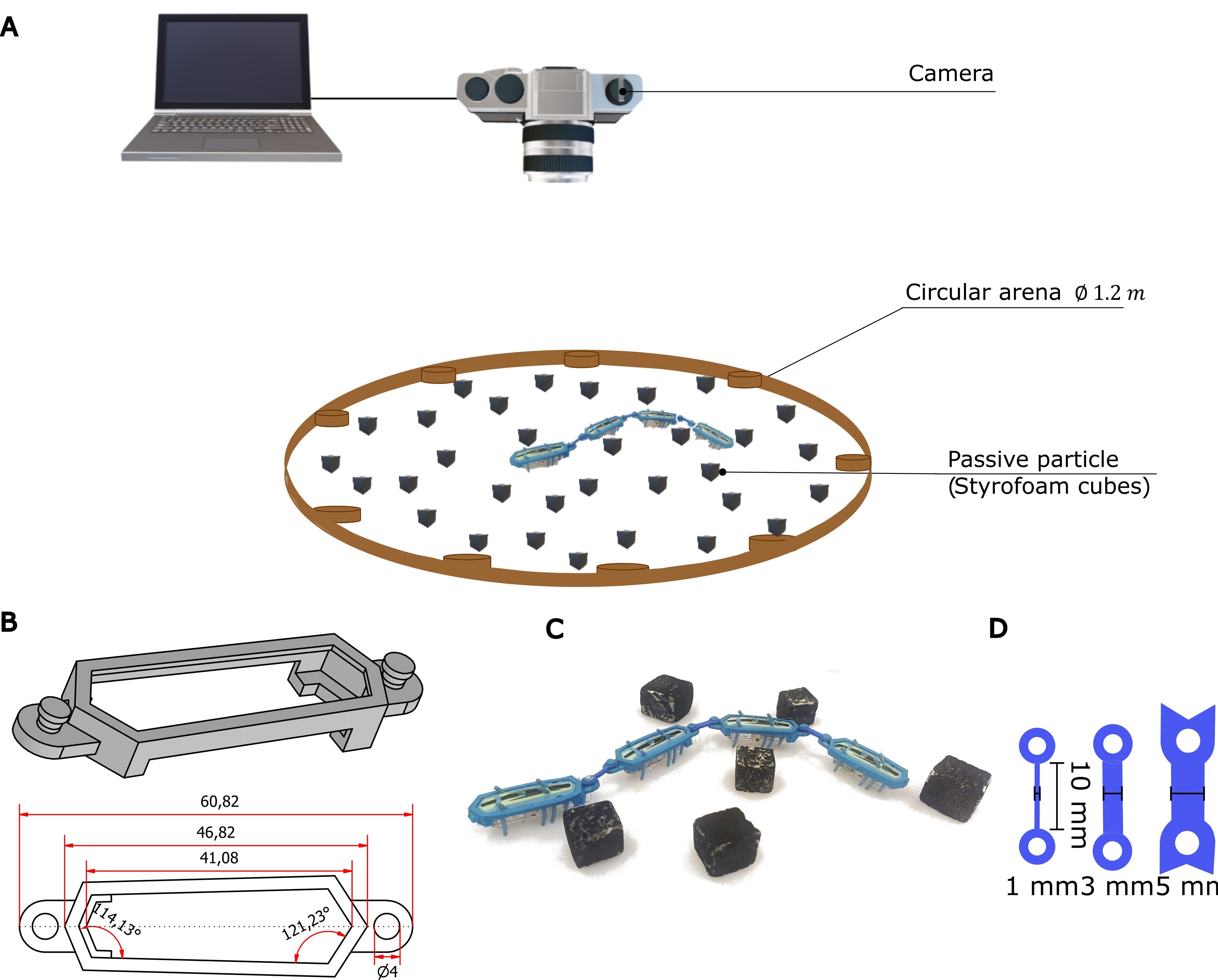
Figure S4: Experimental setup for particle collection with a robotic chain. (A) The circular arena has a diameter of 1.20 m, with nine “re-injectors” evenly spaced around the perimeter. A high-resolution camera is mounted on the ceiling to capture the chain’s conformation, dynamics, and the position of passive particles over time. (B) Schematic with dimensions of the plastic casing that houses the robots. (C) Close-up view of a small chain of robots interacting with the styrofoam cubic particles. (D) The three different types of connectors used in the experiments to modify the design and stiffness of the robotic chain.

	2 bots	6 bots	10 bots	14 bots	18 bots	bending stiffness
1 mm	0.64	0.57	0.33	0.24	0.31	1.52 $\times 10^{-7}$ $Nm^{2}$
3 mm		0.76	0.72	0.47	0.33	4.70 $\times 10^{-6}$ $Nm^{2}$
5 mm	0.67	0.79	0.78	0.50	0.47	1.16 $\times 10^{-5}$ $Nm^{2}$

Table 1: Characteristics of the robotic chains. The average persistence length and bending stiffness of the connectors are reported for the different chain lengths investigated in this work.

I.3 General (data-analyses) methods

In our image analysis, we pursued two main objectives: (i) measuring the size and location of the passive particles that eventually form clusters and (ii) extracting the contour of the filament. In both worm and robotic experiments, the filaments and tracers have distinct colors, allowing for standard thresholding and contour detection algorithms from the Python OpenCV library (https://github.com/opencv/opencv-python) to be largely effective. However, in certain worm experiments, achieving sufficient color contrast proved challenging. In these cases, we employed machine-learning-based segmentation using the YOLO package developed by Ultralytics (https://github.com/ultralytics/ultralytics), which enabled high-precision filament contour detection (model available upon request).

Once the filament contour was identified, the midline—required for measuring the effective persistence length—was extracted using the skeletonization algorithm implemented in the Python scikit-image library (https://github.com/scikit-image/scikit-image). Clusters of tracer particles were detected by identifying the contours of segmented tracers; adjacent tracers sharing a common contour were classified as a single cluster.

To determine the sweep width $W$ as defined in the main text, we superimposed consecutive images until the filament had traversed its full contour length. In the resulting composite image, we identified the largest inscribed circle fully contained within the contour, taking its diameter as the relevant measure of the sweep width. Repeating this procedure over the full duration of an experiment yielded a distribution of $W$ values, from which we report the median as the characteristic sweep width in the main text.

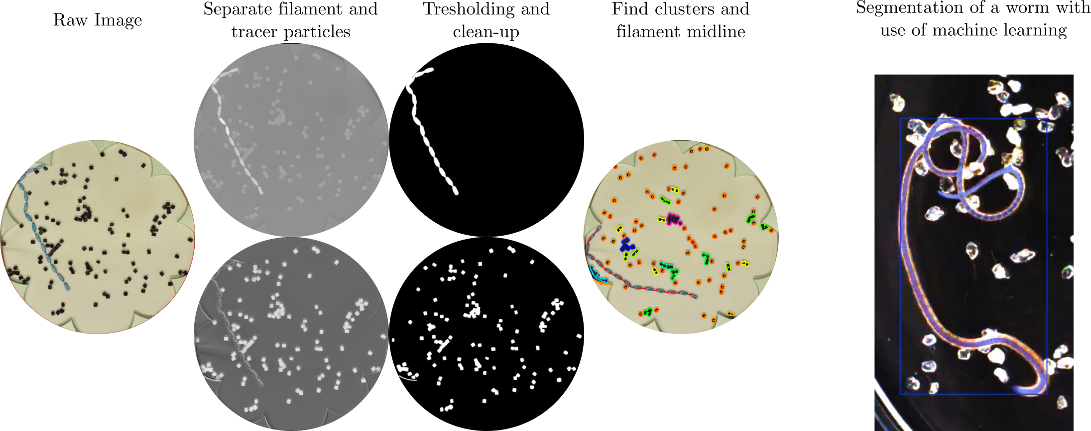
Figure S5: Image analysis protocol for particle tracking and active filament conformation and dynamics. (A) Original experimental image with a white background, black tracer particles, and a blue robotic chain. (B) By selecting the appropriate color channels, the robotic chain is separated from the tracer particles and background. (C) After thresholding and noise filtering, a binary mask of both the filament and tracer particles is obtained. (D) Clusters are identified by detecting the contours of connected tracer particles, while the filament’s midline is extracted using a skeletonization algorithm. (E) Example of the segmentation of a worm, with the use of a machine learning model.

II Models, Simulation details:

In this section, we discuss the details of the simulation used to study a system of passive particles and active polymer.

II.1 Brownian dynamics simulation of Active Polymer and tracers

Here, we consider a $2D$ polymer made of $N$ monomers and $N_{t}$ tracer particles confined to a circular wall made of stationary $N_{b}$ particles as shown in Fig. S7.

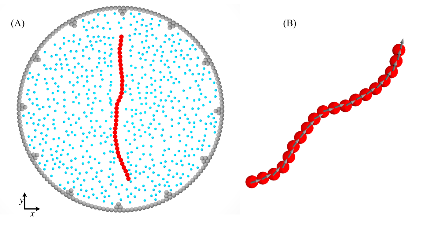
Figure S7: Self-propelling polymer and active polymer model. (A) Self-propelling polymer in the presence of tracer particles confined within a circular boundary. Tracer particles (blue) remain stationary unless displaced by the polymer (connected red beads). The circular boundary consists of fixed gray particles, ensuring confinement. (B) Active polymer model: A tangential active force propels the polymer along its contour. Beads are connected by stiff springs to maintain structural integrity, while a bending potential governs stiffness by penalizing deviations from the preferred angle.

II.1.1 Active polymer

The equation of motion for the particles is,

$$\gamma{{\dot{\bf r}}_{i}}=-\nabla_{i}{{U}^{WCA}}+{\mathcal{A}}(-\nabla_{i}{U}^{stretch}{-\nabla_{i}U}^{bend}+{\bf F}_{i}^{noise}+{\bf F}_{i}^{active})$$ (S1)

The first term corresponds to the steric interactions between all the particles in the systems and is modelled via Weeks-Chandler-Anderson potential [weeks-chandler-71],

$$U^{WCA}(r)=4\varepsilon\left[\left(\frac{\sigma}{r}\right)^{12}-\left(\frac{\sigma}{r}\right)^{6}+\frac{1}{4}\right],$$ (S2)

which vanishes beyond any distance greater than $2^{1/6}\sigma$. Here $\varepsilon$ measures the strength of the repulsive interaction, and is set to $1.0$. $\sigma$ is the size of the particles, we set to monomer size to $1$ and the size of passive tracer to $0.5$. $r\equiv\left|\mathbf{r}_{ij}\right|=\left|\mathbf{r}_{i}-\mathbf{r}_{j}\right|$ is the distance between two beads. The interaction prevents the polymer from crossing different segments of its chain as well as makes passive beads repulsive. Even though wall particles are stationary, when any other particles come within the distance ($2^{1/6}\sigma$), they experience the $U^{WCA}$ interaction and avoid any leakage of the particles through the wall.

Now, we discuss the last term in Eqn. S1 containing contributions from four interactions and is experienced by the polymer beads solely as $\mathcal{A}$ is set to 1 for the polymers and $\mathcal{A}=0$ for tracer particles. Since these interactions are absent for passive particles, we set ${\mathcal{A}}$ to zero for such particles. Each connected pair of the polymer interacts via a harmonic potential [kkremer-90],

$$U_{stretch}(r)=k_{b}\big{(}r-R_{0}\big{)}^{2}.$$ (S3)

Here $R_{0}=1.0\sigma$ is the maximum bond length, and $k_{b}=4000~k_{B}T/\sigma^{2}$ is the bond stiffness. Bending interaction is experienced by any connected triplet in the polymer, and it is given by the potential,

$$U_{bend}=\kappa\big{(}\theta-\theta_{0}\big{)}^{2}$$ (S4)

Here $\kappa$ is the bending stiffness and is related to the continuum bending stiffness, $\tilde{\kappa}$, as $\kappa\approx\tilde{\kappa}/2\sigma$, $\theta$ is the angle between any consecutive bond vectors and $\theta_{0}$ is set to $\pi$. These parameters make the chain effectively inextensible with bond length $b\sim 1\sigma$ and polymer length $L=(N-1)b\sigma$.

The stochastic term ${\bf F}^{noise}_{i}$ represents the thermal fluctuations and is modelled as white noise with zero mean and variance proportional to $\sqrt{k_{B}Tm\xi/\Delta t}$.

We measure length in units of particle size $\sigma$, energies in units of $k_{B}T$, and time in units of $\tau=\sqrt{\frac{m\sigma^{2}}{k_{B}T}}$.

Finally, the last term represents self-propulsion force for the polymer,

$${\bf F}_{i}^{active}=\frac{f_{p}}{2}({\bf\hat{t}}_{i-1,i}+{\bf\hat{t}}_{i,i+1})$$ (S5)

Here, $f_{p}$ is the strength of the force and ${\bf\hat{t}}_{i,i+1}={\bf r}_{i,i+1}/{\bf r}_{i,i+1}$ is the unit tangent vector along the bond connecting beads i and i + 1. This is experienced by the beads ($i=2,3,4...N-1$) of the polymer. The active forces for the end beads ($i=1$ and $i=N$), as they have only one nearest neighbour, are

$${\bf F}_{1}^{active}=\ \hat{\bf t}_{1}f_{p}\;\&\;\;\\ {\bf F}_{N}^{active}=\hat{\bf t}_{N-1}f_{p}$$ (S6)

We set the $\gamma$ for polymers to be 1.0 and $\gamma=10.0$

We also create a confinement using a set of repulsive particles that are stationary.

II.1.2 Effect of particle density

We examined the effect of initial particle density on the long-time average cluster size $\langle s\rangle_{L}$. The results are presented in Sup. Fig. SS8. By normalizing the long-time average cluster size as $(\langle s\rangle_{L}-1)/N_{t}$, we achieve a collapse of all data onto a single curve, effectively capturing the influence of the initial total number of passive particles within the confinement.

II.1.3 Number of Boundary Defects as “Re-injectors”

We investigated the impact of varying the number of boundary defects on particle collection in simulations. As shown in Sup. Fig. S9, the number of defects does not have aot have a significant effect on the ollecting dynamics.

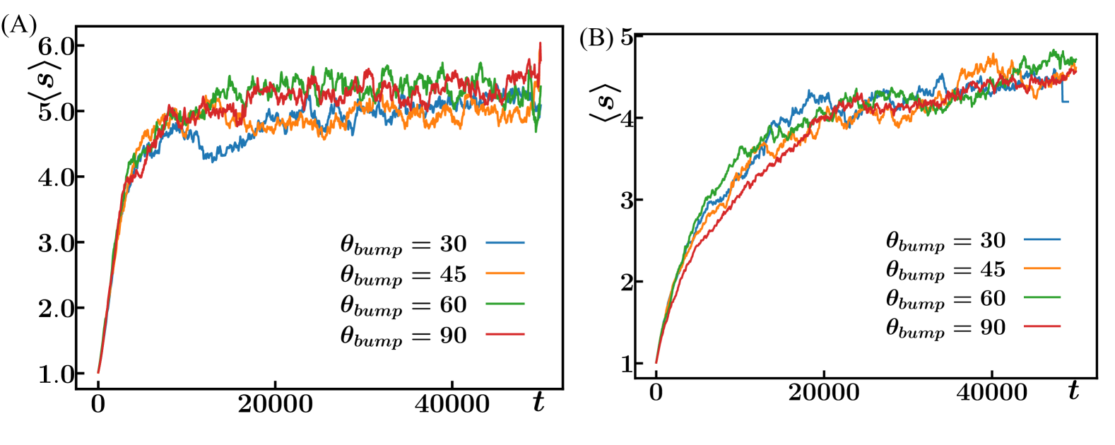
Figure S9: Effect of the number of boundary reflectors on particle collection. (A) Particle collection dynamics for a flexible filament. (B) Particle collection dynamics for a stiff filament.

II.2 Toy model for particle collecting

To gain insight into the underlying mechanisms of particle collection observed in our experiments, we develop a minimal computational model, as discussed in Figure 4 of the main text. This simplified model simulates the collection process in an enclosed arena of size $L\times L$, where passive particles are randomly distributed and displaced by repeated sweeping motions.

We initialize the system as follow: - The arena is represented as a discrete $L\times L$ grid. - A total of $N_{t}$ pixels are randomly selected to represent passive particles, ensuring a dilute regime. - The swipe width is set to $w=2w^{*}+1$, where $w^{*}$ defines a characteristic half-width of the sweeping motion.

After initialization, the simulation proceeds through the following iterative steps:

1. A sweep direction (horizontal or vertical) is chosen randomly with equal probability.

2. A random position $x$ (for vertical sweeps) or $y$ (for horizontal sweeps) is selected within the arena to place the sweep.

3. All tracer particles within the swipe region are displaced:

   • If a particle’s position $x_{t}$ (or $y_{t}$) satisfies $x-w<x_{t}<x$, it is moved leftward (or downward) to $x_{t}\rightarrow x-w-1$.

   • If a particle’s position satisfies $x\leq x_{t}<x+w$, it is moved rightward (or upward) to $x_{t}\rightarrow x+w+1$.

4. If the new location is already occupied, the particle continues moving in the same direction until it reaches an empty spot. In rare cases where no empty spot is found, the simulation terminates.

5. The sizes of particle clusters, defined as aggregates of directly neighboring tracer particles, are measured.

6. A new direction and position are selected, and the process repeats.

For all simulations, the arena size is fixed at $L=100$, while the number of tracer particles $N_{t}$ is varied from 100 to 2000 to explore different densities.

This toy model provides a simple yet effective framework for capturing the essential features of particle aggregation and redistribution driven by sweeping motions.

III Supplementary details

III.1 Effect of persistence length on the sweep width $W$

Longer and more flexible active filaments exhibit larger transverse fluctuations, leading to an increased sweep width $W$. $W$ is measured as explained in section C above. This trend is confirmed in Fig. S10, which shows a systematic increase of the sweep width $W$ with filament length and flexibility. However, one can note that it varies across the different systems.

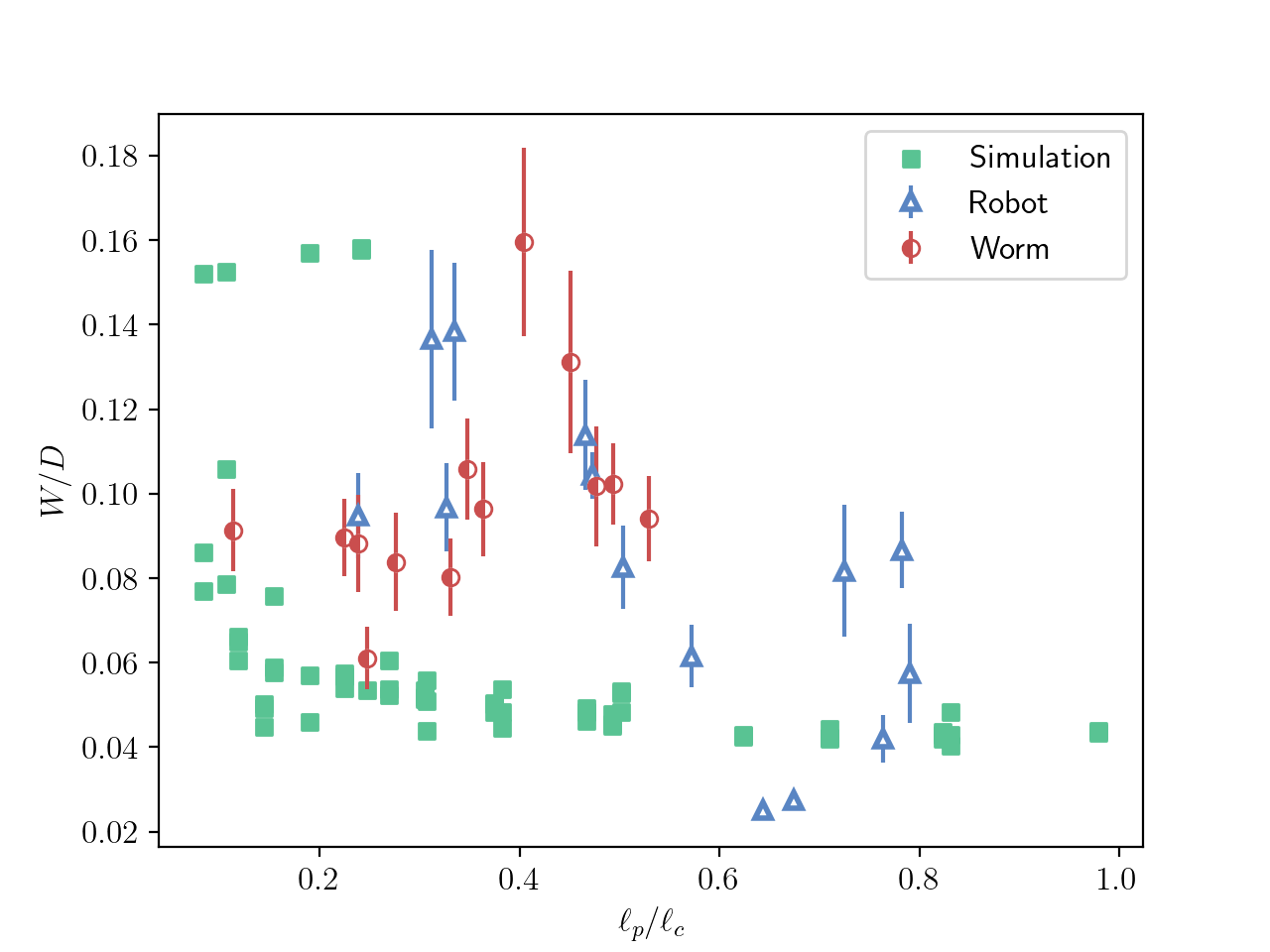
Figure S10: Sweep width $W$ as a function of the normalized persistence length for all active filament systems. The same trend is observed between $W$ and filament flexibility across all systems studied.

III.2 Smoluchowski-coagulation theory

A natural framework to describe the observed aggregation is Smoluchowski aggregation theory [8]. Assuming no fragmentation and that clusters of all sizes interact equally with any other cluster in the system, the dynamics follow:

$$s_{n} =\frac{N_{tot}(t/\tau)^{n-1}}{(1+t/\tau)^{n+1}},$$ (S7)

$$\tau =\frac{2}{k\cdot N_{tot}},$$ (S8)

where $s_{n}$ represents a cluster of size $n$ and $\tau$ is the characteristic aggregation timescale. This relation accurately describes the initial stages of aggregation across all systems (see Fig. S11). However, as time progresses, fragmentation becomes significant, rendering this model insufficient to fully capture the observed dynamics.

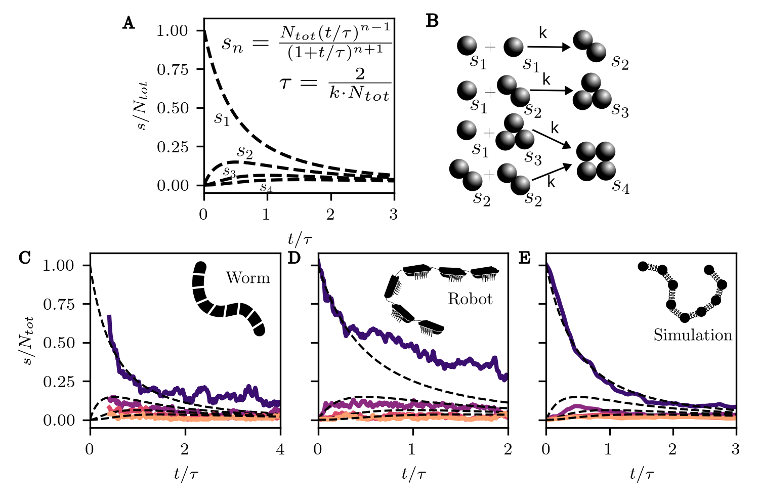
Figure S11: Smoluchowski coagluation for a constant kernel. A Theoretical prediction. B Sketch explaining the terms used. $s_{n}$ denotes a cluster of size $n$, k is the reaction rate. C Fit to the clustering measured for one of the worms D Fit to the clustering measured for one of the robots E Fit to the clustering measured for one of the worms

III.3 Minimal computational model for the collecting process

To validate our minimal simulation model in replicating the sweeping process that leads to particle clustering (Fig. 4 of the main text), we compare the same quantities as in the experimental systems. Figure S12 highlights the relevance of our model in capturing the key clustering dynamics.

Figure S12: A Abundance of particle clusters of sizes 1 to 4 in the minimal model, fitted with Smoluchowski coagulation for a constant kernel. B Cluster size distribution at early, intermediate, and long times, revealing a clear power-law behavior with an exponential cutoff. C Average particle distance from the center of the box for different sweeping widths.

III.4 Cluster Size Distribution

The exponents obtained from the fit of $P(s)=s^{-\gamma}\exp{(-s/s^{*})}$, as reported in Figure 1 of the main text, are as follows:

	Worm	Simulation	Robot	Model
$0t^{*}$	-2.1	-7.2	-6.7	-2.4
$\approx 15t^{*}$	-1.6	-2.3	-2.6	-1.3
$<100t^{*}$	-1.6	-1.3	-1.9	-0.2

While the literature suggests a power-law distribution with an exponential cutoff, our experiments reveal that the clusters do not grow large enough to probe the exponential tail of the distribution. In our minimal model, where the cluster sizes reach higher values, we do observe this cutoff (see Figure S12.B).

References

- Ganguly et al. [2012] S. Ganguly, L. S. Williams, I. M. Palacios, and R. E. Goldstein, Cytoplasmic streaming in drosophila oocytes varies with kinesin activity and correlates with the microtubule cytoskeleton architecture, Proceedings of the National Academy of Sciences 109, 15109 (2012).
- Nédélec et al. [1997] F. Nédélec, T. Surrey, A. C. Maggs, and S. Leibler, Self-organization of microtubules and motors, Nature 389, 305 (1997).
- Sumino et al. [2012] Y. Sumino, K. H. Nagai, Y. Shitaka, D. Tanaka, K. Yoshikawa, H. Chaté, and K. Oiwa, Large-scale vortex lattice emerging from collectively moving microtubules, Nature 483, 448 (2012).
- Goff et al. [2002] L. L. Goff, F. Amblard, and E. M. Furs, Motor-driven dynamics in actin-myosin networks, Phys. Rev. Lett. 88, 018101 (2002).
- Sanchez et al. [2012] T. Sanchez, D. T. Chen, S. J. DeCamp, M. Heymann, and Z. Dogic, Spontaneous motion in hierarchically assembled active matter, Nature 491, 431 (2012).
- Kirchenbuechler et al. [2014] I. Kirchenbuechler, D. Guu, N. A. Kurniawan, G. H. Koenderink, and M. P. Lettinga, Direct visualization of flow-induced conformational transitions of single actin filaments in entangled solutions, Nat. comm. 5, 5060 (2014).
- Sleigh [1962] M. A. Sleigh, The Biology of Cilia and Flagella (Macmillan, New York, 1962).
- Shah et al. [2009] A. S. Shah, Y. Ben-Shahar, T. O. Moninger, J. N. Kline, and M. J. Welsh, Motile cilia of human airway epithelia are chemosensory, Science 325, 1131 (2009).
- Bardy et al. [2003] S. L. Bardy, S. Y. Ng, and K. F. Jarrell, Prokaryotic motility structures, Microbiology 149, 295 (2003).
- Mayfield and Inniss [1977] C. I. Mayfield and W. E. Inniss, A rapid, simple method for staining bacterial flagella, Canadian journal of microbiology 23, 1311 (1977).
- Friedrich et al. [2010] B. M. Friedrich, I. H. Riedel-Kruse, J. Howard, and F. Jülicher, High-precision tracking of sperm swimming fine structure provides strong test of resistive force theory, Journal of Experimental Biology 213, 1226 (2010).
- Deblais et al. [2023] A. Deblais, K. R. Prathyusha, R. Sinaasappel, H. Tuazon, I. Tiwari, V. P. Patil, and M. S. Bhamla, Worm blobs as entangled living polymers: from topological active matter to flexible soft robot collectives, Soft Matter 19, 7057 (2023).
- Patil et al. [2023] V. P. Patil, H. Tuazon, E. Kaufman, T. Chakrabortty, D. Qin, J. Dunkel, and M. S. Bhamla, Ultrafast reversible self-assembly of living tangled matter, Science (2023).
- Gray [1946] J. Gray, The mechanism of locomotion in snakes, Journal of experimental biology 23, 101 (1946).
- Hernández-López et al. [2024] C. Hernández-López, P. Baconnier, C. Coulais, O. Dauchot, and G. Düring, Model of active solids: Rigid body motion and shape-changing mechanisms, Physical Review Letters 132, 238303 (2024).
- Zheng et al. [2023] E. Zheng, M. Brandenbourger, L. Robinet, P. Schall, E. Lerner, and C. Coulais, Self-oscillation and synchronization transitions in elastoactive structures, Physical Review Letters 130, 178202 (2023).
- Xi et al. [2024] Y. Xi, T. Marzin, R. B. Huang, T. J. Jones, and P.-T. Brun, Emergent behaviors of buckling-driven elasto-active structures, Proceedings of the National Academy of Sciences 121, e2410654121 (2024).
- Tuazon et al. [2023] H. Tuazon, C. Nguyen, E. Kaufman, I. Tiwari, J. Bermudez, D. Chudasama, O. Peleg, and M. S. Bhamla, Collecting–gathering biophysics of the blackworm lumbriculus variegatus, Integrative and Comparative Biology 63, 1474 (2023).
- Gokhale et al. [2022] S. Gokhale, J. Li, A. Solon, J. Gore, and N. Fakhri, Dynamic clustering of passive colloids in dense suspensions of motile bacteria, Physical Review E 105, 054605 (2022).
- Dolai et al. [2018] P. Dolai, A. Simha, and S. Mishra, Phase separation in binary mixtures of active and passive particles, Soft Matter 14, 6137 (2018).
- Stenhammar et al. [2015] J. Stenhammar, R. Wittkowski, D. Marenduzzo, and M. E. Cates, Activity-induced phase separation and self-assembly in mixtures of active and passive particles, Phys. Rev. Lett. 114, 018301 (2015).
- McCandlish et al. [2012] S. R. McCandlish, A. Baskaran, and M. F. Hagan, Spontaneous segregation of self-propelled particles with different motilities, Soft Matter 8, 2527 (2012).
- Visser [2007] A. W. Visser, Biomixing of the oceans?, Science 316, 838 (2007).
- Prathyusha [2023] K. R. Prathyusha, Passive particle transport using a transversely propelling polymer “sweeper”, Soft Matter 19, 4001 (2023).
- Zhang et al. [2021] B. Zhang, T. Lei, and N. Zhao, Comparative study of polymer looping kinetics in passive and active environments, Physical Chemistry Chemical Physics 23, 12171 (2021).
- Smrek and Kremer [2017] J. Smrek and K. Kremer, Small activity differences drive phase separation in active-passive polymer mixtures, Physical Review Letters 118, 098002 (2017).
- Deblais et al. [2018] A. Deblais, T. Barois, T. Guerin, P.-H. Delville, R. Vaudaine, J. S. Lintuvuori, J.-F. Boudet, J.-C. Baret, and H. Kellay, Boundaries control collective dynamics of inertial self-propelled robots, Physical Review Letters 120, 188002 (2018).
- Prathyusha et al. [2018] K. R. Prathyusha, S. Henkes, and R. Sknepnek, Dynamically generated patterns in dense suspensions of active filaments, Physical Review E 97, 022606 (2018).
- Isele-Holder et al. [2015] R. E. Isele-Holder, J. Elgeti, and G. Gompper, Self-propelled worm-like filaments: spontaneous spiral formation, structure, and dynamics, Soft Matter 11, 7181 (2015).
- Fazelzadeh et al. [2023] M. Fazelzadeh, Q. Di, E. Irani, Z. Mokhtari, and S. Jabbari-Farouji, Active motion of tangentially driven polymers in periodic array of obstacles, The Journal of Chemical Physics 159 (2023).
- Ozkan-Aydin et al. [2021] Y. Ozkan-Aydin, D. I. Goldman, and M. S. Bhamla, Collective dynamics in entangled worm and robot blobs, Proceedings of the National Academy of Sciences 118, e2010542118 (2021).
- Ginot et al. [2018] F. Ginot, I. Theurkauff, F. Detcheverry, C. Ybert, and C. Cottin-Bizonne, Aggregation-fragmentation and individual dynamics of active clusters, Nature communications 9, 696 (2018).
- Martín-Roca et al. [2024] J. Martín-Roca, E. Locatelli, V. Bianco, P. Malgaretti, and C. Valeriani, Tangentially active polymers in cylindrical channels, SciPost Phys. 17, 107 (2024).
- Sinaasappel et al. [2024] R. Sinaasappel, M. Fazelzadeh, T. Hooijschuur, S. Jabbari-Farouji, and A. Deblais, Locomotion of active polymerlike worms in porous media, arXiv preprint arXiv:2407.18805 (2024).
- Deseigne et al. [2010] J. Deseigne, O. Dauchot, and H. Chaté, Collective Motion of Vibrated Polar Disks, Physical Review Letters 105, 098001 (2010).
- Deseigne et al. [2012] J. Deseigne, S. Léonard, O. Dauchot, and H. Chaté, Vibrated polar disks: spontaneous motion, binary collisions, and collective dynamics, Soft Matter 8, 5629 (2012).
- Patterson et al. [2017] G. A. Patterson, P. I. Fierens, F. Sangiuliano Jimka, P. König, Á. Garcimartín, I. Zuriguel, L. A. Pugnaloni, and D. R. Parisi, Clogging transition of vibration-driven vehicles passing through constrictions, Physical Review Letters 119, 248301 (2017).
- Dauchot and Démery [2019] O. Dauchot and V. Démery, Dynamics of a self-propelled particle in a harmonic trap, Physical Review Letters 122, 068002 (2019).
- Krapivsky et al. [2010] P. L. Krapivsky, S. Redner, and E. Ben-Naim, A Kinetic View of Statistical Physics (Cambridge University Press, 2010).
- Ziff [1980] R. M. Ziff, Kinetics of polymerization, Journal of Statistical Physics 23, 241 (1980).
- Bouvard et al. [2023] J. Bouvard, F. Moisy, and H. Auradou, Ostwald-like ripening in the two-dimensional clustering of passive particles induced by swimming bacteria, Physical Review E 107, 044607 (2023).
- Smoluchowski and im unbegrenzten Raum [1906] V. Smoluchowski and I. D. im unbegrenzten Raum, Zusammenfassende bearbeitungen, Ann. Phys 21, 756 (1906).

References

- [1] H. Tuazon, E. Kaufman, D. I. Goldman, and M. S. Bhamla, “Oxygenation-controlled collective dynamics in aquatic worm blobs,” Integrative and Comparative Biology, vol. 62, no. 4, pp. 890–896, 2022.
- [2] H. Tuazon, C. Nguyen, E. Kaufman, I. Tiwari, J. Bermudez, D. Chudasama, O. Peleg, and M. S. Bhamla, “Collecting–gathering biophysics of the blackworm lumbriculus variegatus,” Integrative and Comparative Biology, vol. 63, no. 6, pp. 1474–1484, 2023.
- [3] H. Tuazon, S. David, K. Ma, and S. Bhamla, “Leeches predate on fast-escaping and entangling blackworms by spiral entombment,” Integr. Comp. Biol., p. icae118, July 2024.
- [4] A. Deblais, S. Woutersen, and D. Bonn, “Rheology of entangled active polymer-like t. tubifex worms,” Physical Review Letters, vol. 124, no. 18, p. 188002, 2020.
- [5] A. Deblais, A. Maggs, D. Bonn, and S. Woutersen, “Phase separation by entanglement of active polymerlike worms,” Physical Review Letters, vol. 124, no. 20, p. 208006, 2020.
- [6] T. Heeremans, A. Deblais, D. Bonn, and S. Woutersen, “Chromatographic separation of active polymer–like worm mixtures by contour length and activity,” Science Advances, vol. 8, no. 23, p. eabj7918, 2022.
- [7] A. Deblais, K. R. Prathyusha, R. Sinaasappel, H. Tuazon, I. Tiwari, V. P. Patil, and M. S. Bhamla, “Worm blobs as entangled living polymers: from topological active matter to flexible soft robot collectives,” Soft Matter, vol. 19, pp. 7057–7069, 2023.
- [8] V. Smoluchowski and I. D. im unbegrenzten Raum, “Zusammenfassende bearbeitungen,” Ann. Phys, vol. 21, p. 756, 1906.