Polluted Modified Bootstrap Percolation

Abstract

In the polluted modified bootstrap percolation model, sites in the square lattice are independently initially occupied with probability $p$ or closed with probability $q$. A site becomes occupied at a subsequent step if it is not closed and has at least one occupied nearest neighbor in each of the two coordinates. We study the final density of occupied sites when $p$ and $q$ are both small. We show that this density approaches $0$ if $q\geq Cp^{2}/\log p^{-1}$ and $1$ if $q\leq p^{2}/(\log p^{-1})^{1+o(1)}$. Thus we establish a logarithmic correction in the critical scaling, which is known not to be present in the standard model, settling a conjecture of Gravner and McDonald from 1997.

1 Introduction

Bootstrap percolation has been extensively studied as a model for nucleation and metastability. In the version considered in this paper, each site in the lattice ${\mathbb{Z}}^{2}$ is in one of the three states: occupied (also called infected), closed (immune), or open (susceptible). Initially, the state of each vertex is chosen independently at random: occupied with probability $p$ and closed with probability $q$, where $p+q\leq 1$. We will assume throughout that the probability parameters $p$ and $q$ are small. After the initial configuration is chosen, it evolves according to a simple deterministic rule in which occupied and closed sites never change their states, but an open site may become occupied. In the standard bootstrap percolation, an open site at time $t$ becomes occupied at time $t+1$ if and only if at least 2 of its 4 nearest neighbors are occupied at time $t$. In the modified version, this transition is further restricted: at each step, every open site that has at least one occupied nearest neighbor to the east or west and at least one occupied nearest neighbor to the north or south becomes occupied.

The standard “unpolluted” case with $q=0$, a variant of which was introduced in [CLR], has played a central role in the study of spatial dynamics in random settings. The first rigorous result, proved in [vE], established that, as soon as $p>0$, every site of ${\mathbb{Z}}^{2}$ is eventually occupied with probability $1$. To probe the metastability properties of the model, a natural setting is to restrict the lattice to a finite square of large side length $n$. This lead to increased understanding of the mechanism for nucleation and the exponential scaling function is now known to a remarkable precision [AL, Hol, GHM, HM, HT]. Many variations were also extensively studied, e.g. [BBDM, BDMS, BBMS1, BBMS2]. A brief survey cannot do justice to the variety and depth of the results in this area, so we refer to the review [Mor] for further background.

The “polluted” standard case with $q>0$ was introduced in [GM]. Here, the main focus is the final density of occupied sites. The main result of [GM] is that there exist constants $c,C>0$ so that when $(p,q)\to(0,0)$,

(1.1) $$\mathbb{P}\left(\text{the origin is occupied}\right)\to\begin{cases}1&\text{if }q<cp^{2}\\ 0&\text{if }q>Cp^{2}\\ \end{cases}$$

Rigorous extensions of this result have been relatively scarce, but higher-dimensional cases [GraH, GHS, DYZ] and general two-dimensional models [Gho] have been addressed recently.

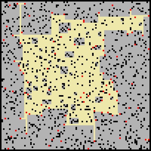
Figure 1: The dynamics with $p=0.1$, $q=0.01$ attempts to fill in a square. Black sites are initially occupied, including all sites on the boundary, grey sites are eventually occupied, and red sites are closed.

For the modified model, the argument in [GM], which proves (1.1) for the standard rule, allows the possibility of a logarithmic correction in the scaling (see also open problem (2) in [GHS]). In this paper, we confirm that, indeed, $p^{2}$ in (1.1) needs to be replaced by $p^{2}/\log p^{-1}$, although we have to allow a possible correction power of $\log\log p^{-1}$ in the lower bound. It is unclear whether such a power can be removed, and we leave this as a natural open question. While the modified model is in many senses similar to the standard one, notably in the dominant exponential term in the nucleation scaling [Hol], there are important differences. The recent result on the scaling correction [Har] is one example, and the present paper provides another. The cause is illustrated in Figure 1, where narrow “chimneys” — one site wide segments of open sites, with closed sites at their ends — block the inward progress of occupation. Unsurprisingly, the chimney phenomenon is closely reflected in our proofs. In the standard rule, occupation can easily invade such chimneys. We now formally state our results.

Theorem 1.1.

There exists a constant $C>0$ so that if $q\geq Cp^{2}/\log(1/p)$, then

(1.2) $$\lim_{q\to 0}\mathbb{P}_{p,q}\bigl{(}(0,0)\text{ is eventually occupied}\,\bigr{)}=0.$$

Theorem 1.2.

If

$$q\leq\frac{p^{2}}{\log(1/p)(\log\log(1/p))^{4}},$$

then

(1.3) $$\lim_{p\to 0}\mathbb{P}_{p,q}\bigl{(}(0,0)\text{ is eventually occupied}\,\bigr{)}=1.$$

We prove these two theorems in the following two sections respectively.

2 Stopping the infection

Fix an odd integer $m\geq 1$ and an integer $k\geq 2$. Fix also $\epsilon,\delta>0$. Let $M=\lfloor\delta p^{-1}\log p^{-1}\rfloor$ and $N=2m\lceil\epsilon/(mp)\rceil$. We partition the lattice into rectangles of width $M$ and height $N$, which we call blocks: for $z=(z_{1},z_{2})\in{\mathbb{Z}}^{2}$, we let $R_{z}=(Mz_{1},Nz_{2})+([0,M-1]\times[0,N-1])$.

A block $R_{z}$ is called safe if there exists an $x$ in the upper half of $R_{z}$ so that:

• $x$ is closed;

• there is a rectangle of width $m$ and height $k\lceil\epsilon p^{-1}\rceil$, whose top edge is included in the top edge of $R_{z}$, contains $x$ within its middle vertical line and contains no initially occupied sites; and

• there is a rectangle of width $k\cdot\lfloor\delta p^{-1}\log p^{-1}\rfloor$ and height $m$, whose left edge is contained within the bottom half of the left edge of $R_{z}$, and contains no initially occupied sites.

Figure 2: A safe block (outlined in blue) has a closed site marked by $\times$ and no occupied sites in the red protective region. Its core is outlined by thicker red lines. Dimensions of rectangles are given with integer parts omitted.

If $R_{z}$ is safe, we call the union of the two rectangles from conditions (S2) and (S3) its protective region; the horizontal and vertical line segments in the middle of the two rectangles together form its core; see Figure 2.

Lemma 2.1.

Fix $m$ and $k$, and any $\eta>0$. Then $\epsilon$, $\delta$ and a constant $C$ can be chosen so that, for any fixed $z$,

$$\mathbb{P}\left(R_{z}\text{ is {\color[rgb]{0,0,0}safe}}\right)\geq 1-\eta,$$

provided that

$$q\geq C\frac{p^{2}}{\log p^{-1}}$$

and $p$ is small enough.

Proof.

Note first that the probability that a fixed rectangle of dimensions in condition (S2) has an occupied site is at most

$${\color[rgb]{0,0,0}p\cdot m\cdot k\cdot\frac{2\epsilon}{p}=2mk\epsilon.}$$

Therefore, the conditional probability that (S2) happens given that (S1) happens is at least $1-\eta/3$ for small enough $\epsilon$. Further, for small $p$,

$$\mathbb{P}\left(\text{{\color[rgb]{0,0,0}(S3)} does not happen}\right) \leq\left[1-(1-p)^{mk\delta p^{-1}\log p^{-1}}\right]^{\epsilon/(mp)}$$

$$\leq\left[1-\exp(-2mk\delta\log p^{-1})\right]^{\epsilon/(mp)}$$

$$=\left[1-p^{2mk\delta}\right]^{\epsilon/(mp)}$$

$$\leq\exp\left[\frac{\epsilon}{m}p^{2mk\delta-1}\right],$$

which goes to $0$ as $p\to 0$ provided that $2mk\delta<1$. Under this condition, (S3) therefore happens with probability at least $1-\eta/3$. Finally,

$$\frac{1}{2}|R_{z}|q\geq{\color[rgb]{0,0,0}\frac{1}{2}}C\epsilon\delta,$$

and so (S1) happens with probability at least $1-\eta/3$ if $C$ is large enough. The claim follows. ∎

Figure 3: Safe blocks are outlined in black, and red lines are the cores of their protective regions. Thicker red lines are the blocking structure. Even if all sites above the blocking structure are occupied, they cannot influence the configuration below the structure without help from additional occupied sites below.

Assume that some fixed configuration $\xi_{0}$ has the following properties. There is a bi-infinite path $\ldots,z_{-1},z_{0},z_{1},z_{2},\ldots$ in ${\mathbb{Z}}^{2}$ such that:

• $R_{z_{\ell}}$ is a safe block for every $z_{\ell}$ in the path;

• the path only makes horizontal or vertical steps in positive directions: $z_{i+1}-z_{i}\in\{e_{1},e_{2}\}$; and

• the path makes at most two consecutive steps in the same direction.

We form a blocking structure from this path of safe blocks as follows. From the last box in each horizontal segment of the path, we include in the blocking structure the part of its core that lies (weakly) below and to the right of the closed site satisfying condition (1) of the safe block; see Figure 3. Let $A\subset{\mathbb{Z}}^{2}$ be the region strictly above the blocking structure. Assume also $k\geq 3$, $m\geq 4$. The following lemma encapsulates the key observation used to prove Theorem 1.1. Its proof is similar to that of Proposition 3.2 in [GS], which is itself a simplified 2-dimensional version of Proposition 4 in [GHS].

Lemma 2.2.

Under the above assumptions, convert the configuration in $A$ to entirely occupied and to entirely closed, respectively, and run the two dynamics, obtaining the final configurations $\xi_{o}$ and $\xi_{c}$, respectively. Provided all connected clusters of occupied sites in $\xi_{c}$ have $\ell^{\infty}$-diameter at most $m/4$, the configurations $\xi_{o}$ and $\xi_{c}$ agree on $A^{c}$.

Proof of Theorem 1.1.

Observe that $R_{z_{1}}$ and $R_{z_{2}}$ are safe independently if $z_{1}$ and $z_{2}$ are at $\ell^{\infty}$-distance at least $\max(k,m)$. Therefore, by [LSS] and Lemma 2.1, the random configuration $\{z:R_{z}\text{ is {\color[rgb]{0,0,0}safe}}\}$ dominates an independent configuration on ${\mathbb{Z}}^{2}$ with density arbitrarily close to $1$ if $C$ is large enough and $p$ is small. The rest of the proof is handled by duality arguments developed in [GH1, GH2, DDG+]. In fact, a minor modification of the argument for Theorem 3.1 in [GS] (using Lemma 2.2 in place of Proposition 3.2 in [GS]) ends the proof. ∎

We remark that we in fact need only vertical chimneys to construct a blocking structure and to combine them into a bounded protective set. Therefore, Theorem 1.1 remains valid if the dynamics also permits occupation of an open site with north and south occupied neighbor. Clearly, by monotonicity, Theorem 1.2 also remains valid in this case.

3 Infecting the origin

The key to our proof of Theorem 1.2 is the fact that, once a closed site is surrounded by occupied sites, it is effectively eliminated; a more precise statement is given in the following lemma.

Lemma 3.1.

Fix $x\in{\mathbb{Z}}^{2}$ and two initial configurations on ${\mathbb{Z}}^{2}$. Assume that the two initial configurations agree off $x$ and both lead to eventual occupation of all four neighbors of $x$. Then the resulting final configurations also agree off $x$.

Proof.

The neighbors of $x$ become occupied eventually, so we may assume that they are initially occupied in both dynamics. Since no other vertex has $x$ as a neighbor, its state is now irrelevant for either of the dynamics. ∎

To infect the origin, we partition the lattice into square boxes of side length $N=\lfloor n\cdot\frac{1}{p}\log(1/p)\rfloor$: for $z\in{\mathbb{Z}}^{2}$, $B_{z}=Nz+[0,N-1]^{2}$. Here, $n=n(p)$ is a quantity that goes to $\infty$ as $p\to 0$ and will be chosen later. We now call a box $S$ good if the following conditions hold.

• No two closed sites in $S$ are within $\ell^{\infty}$-distance $2\lceil n/p\rceil$.

• Every closed site $x\in S$ has an occupied site in each of the four lattice directions within distance $\lceil n/p\rceil$ and inside $S$.

• Every horizontal and vertical interval of length $\lfloor 3p^{-1}\log p^{-1}\rfloor$, included in $S$, contains an occupied site.

• Every strip of width $\lfloor np^{-1}\log p^{-1}\rfloor$ and height $\lfloor n^{2}p^{-1}\rfloor$, included in $S$, contains at most $n/4$ closed sites.

• There are no closed sites within distance $2\lceil n/p\rceil$ from the boundary of $S$.

• Every row and every column within $S$ contains at most one closed site.

In fact, (G6) is not needed for the next lemma, but it is easy to achieve and we add it to make the proof a little simpler.

Figure 4: The box $S$ and its subregions. The name of each subregion is at its top right corner. The outline of $S_{1}$ is thicker. Integer parts are again omitted.

The sites outside a box $S$ that have a neighbor in $S$ are divided into four sides, which we call the outside boundary intervals of $S$.

Lemma 3.2.

Under conditions (G1)–(G6), if an outside boundary interval of $S$ gets completely occupied, then every non-closed site of $S$ also gets occupied.

Proof.

If there are no closed sites in $S$, the claim follows from the fact that every row and column of $S$ contains an occupied site by condition (G3). Otherwise, we claim that there exists a closed site in $S$ such that all four of its neighbors eventually become occupied. By Lemma 3.1, we may eliminate this closed site by changing its status to occupied. As conditions (G1)–(G6) are preserved when a closed site is converted to occupied, the claim ends the proof, and in the remainder of the argument we establish this claim.

We may assume that the outside interval adjacent to the bottom of $S$ is occupied. We denote $r=\lceil n/p\rceil$. We will now define several subregions of $S$, illustrated in Figure 4. Let $S_{1}$ be the $\lfloor np^{-1}\log p^{-1}\rfloor\times\lfloor n^{2}p^{-1}\rfloor$ strip on the bottom of $S$. We may assume that $S_{1}$ contains at least one closed site or it becomes completely occupied and we may replace $S_{1}$ with a vertical translate of $S_{1}$ by $\lfloor n^{2}p^{-1}\rfloor$. We conclude from (G4) that, within $S_{1}$, there is a strip $S_{2}$ of width at least

$$\frac{{\color[rgb]{0,0,0}\lfloor np^{-1}\log p^{-1}\rfloor}}{n/4+1}\geq 3p^{-1}\log p^{-1}$$

and the same height as $S_{1}$ with no closed sites. By (G3), $S_{2}$ gets entirely occupied. Also, as

$$\frac{{\color[rgb]{0,0,0}\lfloor n^{2}p^{-1}\rfloor}}{n/4+1}>r,$$

there is a horizontal strip $S_{3}$ within $S_{1}$ of the same width as $S_{1}$ and height at least $r$ that contains no closed sites. Let $S_{4}$ and $S_{5}$ be the left and right components of $S_{1}\setminus(S_{2}\cup S_{3})$ below $S_{3}$. If neither of $S_{4}$, $S_{5}$ contains a closed site (in particular, if they are empty), then all the sites in $S$ up to the top of $S_{3}$ become occupied and we may again translate $S_{1}$ upwards and repeat the setup. Therefore, we assume, without loss of generality, that there is a closed site in $S_{4}$. (See Figure 4.) For any site $z\in S_{4}$ such that $z-e_{2}$ is also in $S_{4}$, we denote by $R(z)$ the rectangle with sides parallel to the axes, and with two of its corners at $z-e_{2}$ and the lower right corner of $S_{4}$. If $z-e_{2}$ is not in $S_{4}$, then we let $R(z)$ be the empty set.

Figure 5: Elimination of a closed site, marked by the red $\times$, at $x$. The dark grey region becomes occupied either by the assumption (the bottom portion) or because it is a part of $S_{2}$ (the right portion). The light grey region — the dashed rectangle is $R(x-re_{1})$ — includes no closed site, and thus also becomes occupied. Each of the four arms of the cross has length $r$, includes an initially occupied site (a black circle) but no closed sites, and thus also becomes occupied.

Pick the closed site $x_{1}\in S_{4}$ closest to $S_{2}$; note that $x_{1}$ is unique by (G6). If $R(x_{1}-re_{1})$ contains no closed site, then all four neighbors of $x_{1}$ become occupied by (G1), (G2) and (G5), and since the height of $S_{3}$ is at least $r$ (see Figure 5). Otherwise, choose the unique closed site $x_{2}\in R(x_{1}-re_{1})$ that is closest to $S_{2}$. By (G1), $x_{2}$ is at distance more than $r$ from the horizontal line containing $x_{1}$. Then, if $R(x_{2}-re_{1})$ contains no closed sites, all four neighbors of $x_{2}$ become occupied by (G1) and (G2). Otherwise, we pick a closed site $x_{3}\in R(x_{2}-re_{1})$, and proceed in the same fashion. As this process cannot continue indefinitely, we eventually find a closed site $x_{\ell}$, whose $R(x_{\ell}-re_{1})$ contains no closed sites, and consequently the four neighbors of $x_{\ell}$ get occupied, as claimed. ∎

Lemma 3.3.

If $n=\lfloor\log\log p^{-1}\rfloor$ and

$$q\leq\frac{p^{2}}{\log p^{-1}\cdot n^{4}},$$

then the probability that a box is good goes to $1$ as $p\to 0$.

Proof.

We have, for some constant $C$,

$$\mathbb{P}\left(\text{{\color[rgb]{0,0,0}(G1)} fails}\right)\leq C\left(\left(\frac{n}{p}\right)^{2}q\right)^{2}\cdot\left(\frac{n\log p^{-1}}{p}\cdot\frac{p}{n}\right)^{2}=C\left(\frac{n^{2}\log p^{-1}}{p^{2}}\cdot q\right)^{2}\leq\frac{C}{n^{4}}\to 0.$$

Next,

$$\mathbb{P}\left(\text{{\color[rgb]{0,0,0}(G2)} fails}\right)\leq\left(\frac{n\log p^{-1}}{p}\right)^{2}\cdot q\cdot 4(1-p)^{n/p}\leq 4\,\frac{\log p^{-1}}{n^{2}}e^{-n}\leq 4{\color[rgb]{0,0,0}e}\,\frac{1}{n^{2}}\to 0.$$

Next, again for some constant $C$,

$$\mathbb{P}\left(\text{{\color[rgb]{0,0,0}(G3)} fails}\right) \leq C\left(\frac{n\log p^{-1}}{p}\cdot\frac{n\log p^{-1}}{p}\cdot\frac{p}{\log p^{-1}}\right)\cdot(1-p)^{3\log p^{-1}/p}$$

$$\leq C\,\frac{n^{2}\log p^{-1}}{p}e^{-3\log p^{-1}}=Cn^{2}p^{2}\log p^{-1}\to 0.$$

Next, for some constant $C$,

$$\mathbb{P}\left(\text{{\color[rgb]{0,0,0}(G4)} fails}\right) \leq C\left(\frac{n\log p^{-1}}{p}\cdot\frac{p}{n^{2}}\right)\cdot\left(\frac{n^{3}\log p^{-1}}{p^{2}}\cdot q\right)^{n/4}$$

$$\leq C\log p^{-1}\cdot\left(\frac{1}{n}\right)^{n/4}$$

$$\leq C\left(\frac{e^{4}}{n}\right)^{n/4}\to 0.$$

Finally,

$$\mathbb{P}\left(\text{{\color[rgb]{0,0,0}(G5)} fails}\right)\leq{\color[rgb]{0,0,0}C}\,\left(\frac{n}{p}\right)^{2}\log p^{-1}\cdot q\leq Cn^{-2}\to 0.$$

and

$$\mathbb{P}\left(\text{{\color[rgb]{0,0,0}(G6)} fails}\right) \leq C\,\frac{n\log p^{-1}}{p}\cdot\left(\frac{n\log p^{-1}}{p}\cdot q\right)^{2}\leq\log p^{-1}\cdot p\to 0.$$

∎

Proof of Theorem 1.2.

Note that the boxes $B_{z}$ are good independently for different $z$. Therefore, by Lemma 3.3, with probability converging to $1$ as $p\to 0$, the set $\{z\in{\mathbb{Z}}^{2}:B_{z}\text{ is good}\}$ contains an infinite connected (in the usual ${\mathbb{Z}}^{2}$ sense) set ${\mathcal{C}}$ that includes the origin. Also with probability converging to $1$ as $p\to 0$, $(0,0)\in R_{0}$ is not closed. With probability 1, there is a site $z\in{\mathcal{C}}$ such that $R_{z}$ is initially completely occupied. By Lemma 3.2, the origin eventually becomes occupied. ∎

References

- [AL] M. Aizenman and J. L. Lebowitz. Metastability effects in bootstrap percolation. Journal of Physics A: Mathematical and General 21 (1988), 3801–3813.
- [BBDM] J. Balogh, B. Bollobás, H. Duminil-Copin, and R. Morris. The sharp threshold for bootstrap percolation in all dimensions. Transactions of the American Mathematical Society, 364 (2012), 2667–2701.
- [BDMS] B. Bollobás, H. Duminil-Copin, R. Morris, and P. Smith. Universality of two-dimensional critical cellular automata. Proceedings of London Mathematical Society 126 (2023), 620–703.
- [BBMS1] P. N. Balister, B. Bollobás, R. Morris, P. Smith, Universality for monotone cellular automata. arXiv:2203.13806.
- [BBMS2] P. N. Balister, B. Bollobás, R. Morris, P. Smith, The critical length for growing a droplet. arXiv:2203.13808.
- [CLR] J. Chalupa, P. L. Leath, and G. R. Reich. Bootstrap percolation on a Bethe lattice. Journal of Physics C: Solid State Physics, 12 (1979), L31.
- [DDG+] N. Dirr, P. W. Dondl, G. R. Grimmett, A. E. Holroyd, and M. Scheutzow. Lipschitz percolation. Electronic Communications in Probability, 15 (2010), 14–21.
- [DYZ] J. Ding, P. Yang, Z. Zhuang. Dynamical random field Ising model at zero temperature. arXiv:2410.20457.
- [GH1] G. R. Grimmett and A. E. Holroyd. Plaquettes, spheres, and entanglement. Electronic Journal of Probability, 15 (2010) 1415–1428, 2010.
- [GH2] G. R. Grimmett and A. E. Holroyd. Geometry of Lipschitz percolation. Annales de l’institut Henri Poincaré (B) Probability and Statistics, 48 (2012), 309–326.
- [GHM] J. Gravner, A. E. Holroyd, and R. Morris. A sharper threshold for bootstrap percolation in two dimensions. Probability Theory and Related Fields, 153 (2012), 1–23.
- [Gho] A. Ghosh, Polluted -bootstrap percolation, Ph.D. Thesis (2022), The Ohio State University, ProQuest Dissertation Publishing 30360081.
- [GHS] J. Gravner, A. E. Holroyd, and D. Sivakoff. Polluted bootstrap percolation in three dimensions, Annals of Applied Probability 31 (2021), 218–246.
- [GM] J. Gravner and E. McDonald. Bootstrap percolation in a polluted environment. Journal of Statistical Physics, 87 (1997), 915–927.
- [GraH] J. Gravner, A. E. Holroyd. Polluted bootstrap percolation with threshold 2 in all dimensions. Probability Theory and Related Fields 175 (2019), 467–486.
- [GS] J. Gravner and D. Sivakoff. Bootstrap percolation on the product of the two-dimensional lattice with a Hamming square. Annals of Applied Probability 30 (2020), 145–174.
- [Har] I. Hartarsky. Sensitive bootstrap percolation second term. Electronic Communications in Probability, 28 (2023), 1–7.
- [HM] I. Hartarsky and R. Morris. The second term for two-neighbour bootstrap percolation in two dimensions. Transactions of the American Mathematical Society 372 (2019), 6465–6505.
- [Hol] A. E. Holroyd. Sharp metastability threshold for two-dimensional bootstrap percolation. Probability Theory and Related Fields, 125 (2003), 195–224.
- [HT] I. Hartarsky and A. Teixeira. Bootstrap percolation is local. arXiv:2404.07903.
- [LSS] T. M. Liggett, R. H. Schonmann, and A. M. Stacey. Domination by product measures. Annals of Probability, 25 (1997), 71–95.
- [Mor] R. Morris. Bootstrap percolation, and other automata. European Journal of Combinatorics 66 (2017), 250–263.
- [vE] A. C. D. van Enter. Proof of Straley’s argument for bootstrap percolation. Journal of Statistical Physics, 48 (1987), 943–945.