Phase transitions and finite-size effects in integrable virial statistical models

Abstract

We analyze thermodynamic models for fluid systems in equilibrium based on a virial expansion of the internal energy in terms of the volume density. We prove that the models, formulated for finite-size systems with $N$ particles, are exactly solvable to any expansion order, as expectation values of physical observables (e.g., volume density) are determined from solutions to nonlinear C-integrable PDEs of hydrodynamic type. In the limit $N\to\infty$, phase transitions emerge as classical shock waves in the space of thermodynamic variables. Near critical points, we argue that the volume density exhibits a scaling behavior consistent with the Universality Conjecture in viscous transport PDEs. As an application, we employ our framework to nuclear matter and construct a global QCD phase diagram revealing critical points for the nuclear liquid-gas and hadron gas–QGP transitions. We demonstrate how finite-size effects smear critical signatures, indicating the importance of thoughtful considerations in the search for the QCD critical point.

Introduction—Understanding phase transitions in matter is a fundamental subject in physics. The presence of interparticle interactions, as well as the involvement of several thermodynamic functions, can result in effects at different scales, with possible multiple critical points and distinct ground states. Variation of a thermodynamic function, such as temperature or pressure, can suppress one phase while promoting another, unveiling a rich interplay between competing phases ParisiRevModPhys.95.030501 ; Ibrahimoglu ; Zhengbook ; PELISSETTO2002549 . Such phenomena are ubiquitous in systems like semiconductors PhysRevLett.44.182 , crystal field SumedhaPRE2020 , spin systems PhysRevLett.69.221 , polymorphic fluids LLScience2020 ; LLPRL2022 , and matter in quantum chromodynamics (QCD) PhysRevC.82.055205 ; FerreiraPRD2018 . Despite the numerous advances in extensive theoretical and experimental studies of these systems, there remains however a need for viable phenomenological approaches and global exact results beyond the regime of the critical point and the thermodynamic limit (TL), which currently rely on heavy numerical simulations.

In this Letter, we analyze the thermodynamics of fluid systems where the nontrivial interactions among particles result into an effective potential energy in the form of a virial-like expansion in the order parameter. Our approach, inspired by papers MORO2014 ; BARRA2015290 , will enable us to identify partial differential equations (PDEs) for the associated statistical models, and to predict behavior of their solutions globally and locally even beyond TL, when finite-size effects are foreseen YangLee_PhysRev.87.404 ; ruelle ; Borrmann_PhysRevLett.84.3511 ; Bernhardt:2021iql ; Kovacs:2023kbv ; LorenzoniPhysRevE.100.022103 . Such effective statistical models provide a simple yet powerful description for van der Waals (vdW) or more imperfect fluid systems across various areas of physics, including classical liquid-gas (L-G) systems callen , the rotating or charged AdS black holes Chamblin:1999tk , astrophysical objects Oertel , ultracold quantum gases Chin_2010 and, last but not least, dense nuclear and quark matter in QCD Kapusta:2006pm where the finite size effects are expected to be significant – the major motivation for this work.

Virial-like statistical models—Phase transitions are conveniently studied within the framework of equilibrium statistical mechanics, which is fundamentally based on the maximum entropy principle callen . This principle turns into an extremity problem for the proper entropic potential $\Psi$ for a specific statistical ensemble, which is related to the system’s entropy $S$ – the relevant potential in the microcanonical ensemble whose natural variables are a set of conserved quantities denoted by vector $\Lambda$ – by Legendre transform $\Psi(\tau)=\sup_{\Lambda}\,[-S(\Lambda)+\tau\Lambda]$, where $\tau\Lambda=\sum_{j=1}^{J}\tau_{j}\Lambda_{j}$ is a product of $J$ conjugate pairs $\{\Lambda_{j},\tau_{j}\}$. The probability of any available microscopic state labeled by $i$ is weighed as $p_{i}=e^{-\tau\Lambda^{(i)}}/{\mathcal{Z}}$, normalized by the partition function associated with the potential $\Psi(\tau)$ to ensure $\sum_{i}p_{i}=1$:

$$\mathcal{Z}=e^{-\Psi(\tau)}=\sum_{i}e^{-\tau\Lambda^{(i)}}\propto\int d\Lambda\,e^{S(\Lambda)-\tau\Lambda}\,,$$ (1)

where in the last step we have taken the continuum limit of the summation over all microscopic states to the integration over $d\Lambda=d\Lambda_{1}\dots d\Lambda_{J}$ and dropped a multiplicative constant. Once the partition function for a given system is assigned, all thermodynamic properties follow in principle lebellac .

For a generic hard spheres fluid system, the microcanonical entropy (up to irrelevant constants) has the well-known form

$$S(E,V,N)=N\ln\left[\frac{V-Nb}{N}\left(\frac{E-U(V,N)}{N}\right)^{\frac{3}{2}}\right]\,,$$ (2)

which depends on its natural (extensive) variables such as internal energy $E$, volume $V$, and particle number $N$. The parameter $b$ identifies the minimum volume density of the configurations in the ensemble. The total potential energy $U$ is assumed a virial-type form

$$U(V,N)=-\sum_{j=1}^{m}\frac{N^{j+1}a_{j+1}}{jV^{j}}\,,$$ (3)

where the virial expansion coefficients $a_{j}$, for $j=1,\cdots,m$, are real constants, since for hard core (or short range) potentials, these coefficients do not (approximately) depend on temperature. The case $m=1$ reproduces the potential energy of the celebrated vdW model. From a mean-field perspective, the potential $U$ can be seen to account for the dependence of the averaged particles interaction upon their average distance $\bar{r}\sim v^{1/3}$, where $v\equiv V/N$ denotes the volume density.

For the case considered in this Letter, where the energy $E$ and volume $V$ of the fluids vary while the particle number $N$ is kept fixed, it is more convenient to consider the isothermal–isobaric ensemble where its natural (intensive) variables, $t=(\partial_{E}S)_{V}$ and $x=(\partial_{V}S)_{E}$, control the fluctuations of energy and volume respectively. In terms of standard pressure $P$ and temperature $T$, $t=1/T$ and $x=P/T$. This choice has been shown to arise naturally in the treatment of vdW MORO2014 ; BARRA2015290 and nematic fluids DEMATTEIS2018 . Thus we are led to consider the scaled Gibbs free energy (i.e., Gibbs free energy divided by temperature)

$$\mathcal{G}_{N}(t,x)\equiv\mathcal{G}(t,x;N)=\sup_{E,V}\,[-S(E,V,N)+tE+xV],$$ (4)

from which the partition function is defined by

$$\mathcal{Z}_{N}(t,x)\equiv e^{-\mathcal{G}_{N}(t,x)}=\int dEdV\,e^{S(E,V,N)-tE-xV}.$$ (5)

Since $U=U(V,N)$, the integration over $E$ accounts only for the kinetic part $K=E-U$. This contributes an irrelevant normalization factor $c(t)\propto t^{-3N/2}$ to the partition function (5), provided that the observables $O$ under consideration are independent of $K$. Consequently, the integration in Eq. (5) reduces to one over all ensemble configurations labeled by $V$ (or $v$ for fixed $N$) alone and one can define another partition function $Z_{N}$ via $\mathcal{Z}_{N}=c(t)Z_{N}$:

$$Z_{N}(t,x)\equiv e^{-G_{N}(t,x)}=\int dv\,e^{-N\psi(t,x;v)}\,,$$ (6)

where $G_{N}$ denotes the associated free energy and

$$\psi(t,x;v)=-s(v)+t\epsilon(v)+xv$$ (7)

is a potential density function. The expectation value of observable $O_{N}(v)=O(V,N)$ is thus given by

$$\langle O_{N}\rangle=\frac{1}{Z_{N}}\int dv\,e^{-N\psi(t,x;v)}O_{N}(v)\,.$$ (8)

Accordingly, we focus on the configurational entropy and potential energy density, given by

$$s(v)=\ln(v-b)\,,\quad\epsilon(v)=-\sum_{j=1}^{m}\frac{a_{j+1}}{jv^{j}}\,,$$ (9)

which result from Eqs. (2) and (3) respectively, and depend only on $v$.

One key observation of our work is that the partition function (6) fulfills the $(m+1)-$th order linear PDE:

$$\left(\partial_{x}^{m}\partial_{t}+\sum_{j=1}^{m}\frac{(-N)^{j+1}a_{j+1}}{j}\partial_{x}^{m-j}\right)Z_{N}(t,x)=0\,.$$ (10)

Eq. (10) is singular in TL $N\to\infty$. It is therefore convenient to identify the differential problem for the free energy density $g_{N}\equiv G_{N}/N$ via Eq. (6). Direct computations give the following nonlinear PDE:

$$B_{m}\partial_{t}g_{N}\\ +\,\sum_{j=1}^{m}B_{m-j}\,\left[\binom{m}{j}\partial_{x}^{j}\partial_{t}g_{N}+\frac{(-N)^{j}a_{j+1}}{j}\right]=0\,,$$ (11)

where $B_{n}=n!\sum_{\{\lambda^{(n)}_{\bf j}\}}\,\prod_{i=1}^{n}\frac{1}{(i!)^{j_{i}}j_{i}!}\left(-N\partial^{i}_{x}g_{N}\right)^{j_{i}}$ is the $n$-th complete exponential Bell polynomial and the summation is performed over all index partitions $\lambda^{(n)}_{\bf j}=\{j_{1},\dots,j_{n}\}$ satisfying $\sum_{i=1}^{n}ij_{i}=n$. When $n=0$, one has, by definition, $B_{0}=1$. The averaged volume density and energy density are simply defined via the derivative of $g_{N}$ as

$${\rm v}_{N}\equiv\langle v_{N}\rangle=\partial_{x}g_{N}\,,\quad\varepsilon_{N}\equiv\langle\epsilon_{N}\rangle=\partial_{t}g_{N}\,,$$ (12)

which allows us to convert Eq. (11) into a PDE for ${\rm v}_{N}$. It follows immediately from Eq. (12) that $\partial_{t}{\rm v}_{N}=\partial_{x}\varepsilon_{N}$.

We emphasize that the PDE (10) for the partition function is linear for the whole family of statistical models admitting the arbitrary virial-like expansion (3). Since physical observables connect to the partition function by transformations involving variable changes and derivatives such as those in Eq. (12), the statistical models under consideration are therefore integrable (more precisely C-integrable Calogero1991WhyAC ).

Multiple phases at large $N$—In the TL $N\to\infty$, letting $g_{N}\to g,{\rm v}_{N}\to{\rm v},\varepsilon_{N}\to\varepsilon$ and inserting it into Eq. (11), one obtains the identity $\varepsilon=\partial_{t}g=\epsilon(\partial_{x}g)=\epsilon({\rm v})$, where Eq. (9) is used. Applying Eq. (12), one arrives at the following local conservation law for the volume density in TL:

$$\partial_{t}{\rm v}-\epsilon^{\prime}({\rm v})\,\partial_{x}{\rm v}=0\,.$$ (13)

This is the Maxwell closure relation for the Gibbs free energy in TL. Its general solution can be obtained via the method of characteristics, yielding $x+t\epsilon^{\prime}({\rm v})-f({\rm v})=0$ where $f({\rm v})$ is an arbitrary function which can be specified by assigning the Cauchy condition, as for instance, if a particular isothermal curve is known in some thermodynamic regimes (such as possibly known isotherms $x=f({\rm v}_{0})$ in the regime of very high temperature). Notice that the function $f$ relates to the function $s$ in Eq. (7) as $f({\rm v})=s^{\prime}({\rm v})$. Indeed, by employing the saddle-point approximation to $Z_{N}$, we get

$$Z_{N}(t,x)\simeq\sum_{\ell}\sqrt{\frac{2\pi}{N\psi^{\prime\prime}_{\ell}}}e^{-N\psi_{\ell}}\,,$$ (14)

where the sum runs over the local minima of the potential $\psi$ defined in Eq. (6), $\psi_{s}\equiv\psi(t,x;{\rm v}_{\ell})$, with $\ell$ labeling the saddle points ${\rm v}_{\ell}$ at which

$$C({\rm v};t,x)\equiv\partial_{\rm v}\psi=x+t\epsilon^{\prime}({\rm v})-s^{\prime}({\rm v})=0\,.$$ (15)

Evidently, Eq. (15) is just the implicit solution to Eq. (13) upon identification $f({\rm v})=s^{\prime}({\rm v})$. The implicit solutions given by $C({\rm v})=0$ represent changes of the volume density of the nonlinear-wave type, which generically undergo a gradient catastrophe whitham ; Thom that emerges at the inflection points (i.e., thermodynamic critical point) MORO2014 , identified by the conditions

$$C({\rm v})=C^{\prime}({\rm v})=C^{\prime\prime}({\rm v})=0\,.$$ (16)

As discussed in MORO2014 ; BARRA2015290 ; Giglio2016IntegrableEV , thermodynamic critical points represent the onset of classical (viscous) shock waves whitham where order parameters and/or their derivatives experience jumps, hence unveiling the occurrence of phase transitions. However, when multiple solutions exist, the equation of state (EOS) does not contain information on which one is the most likely to occur. From a nonlinear wave viewpoint, this problem is equivalent to that of shock fitting, i.e., replacing a multi-valued solution with a discontinuous one (a shock wave), with the discontinuity located according to some specific entropic criteria (cf. Maxwell construction) Bressan .

In TL, multiple solutions of EOS (15), associated with different thermodynamic phases, may exist. A criterion for identifying the favored solution discerns from Eq. (14), which for very large $N$ yields

$${\rm v}_{N}(t,x)\simeq\frac{\sum_{k}{\rm v}_{k}(t,x)(\psi^{\prime\prime}_{k})^{-\frac{1}{2}}\,e^{-N\psi_{k}}}{\sum_{\ell}(\psi^{\prime\prime}_{\ell})^{-\frac{1}{2}}\,e^{-N\psi_{\ell}}}\simeq\bar{\rm v}_{m}(t,x)\,,$$ (17)

where $\bar{\rm v}_{m}(t,x)$ is the solution to $\psi^{\prime}=0$ that corresponds to the lowest minimum of potential $\psi({\rm v})$. Therefore, the phase diagram is identified by selecting the global minimum for each pair of $t$, and will display coexistence curves when two minima are resonant, that is when $\psi_{j}=\psi_{k}$ for two distinct ${\rm v}_{j}$ and ${\rm v}_{k}$. Reconstructing coexistence lines $\mathcal{L}_{jk}\equiv\{(t,x)\in\mathbb{R}^{+}\times\mathbb{R}\,\,|\,\,\psi^{\prime}({\rm v}_{j})=\psi^{\prime}({\rm v}_{k})=0,\,\,\psi({\rm v}_{j})=\psi({\rm v}_{k})\}$ for pairs $j\neq k$, is mathematically equivalent to the problem of tracking trajectories of the underlying shock wave MORO2014 ; Giglio2016IntegrableEV ; callen . When $L$ equally deep lowest minima exist, Eq. (17) implies that all of them contribute to the large $N$ asymptotic solution for the volume density, with those exhibiting the flattest convex shapes in $\psi$ contributing the most. Indeed, from Eq. (17), we get ${\rm v}_{N}\simeq\sum_{\ell=1}^{L}\gamma_{\ell}{\rm v}_{\ell}$ as $N\to\infty$, where the $\gamma_{k}$’s are weights defined by $\gamma_{k}=(\psi^{\prime\prime}_{k})^{-\frac{1}{2}}/\sum_{\ell=1}^{L}(\psi^{\prime\prime}_{\ell})^{-\frac{1}{2}}$. Being single-valued and continuous, this asymptotic solution gives a volume density which lies on the isothermal curve, representing an actual state of the system, differently from the case for multiphase systems callen .

Universality near the critical points—In the large but finite $N$ limit, following Eqs. (11) and (12), one finds that the leading correction to the equation for volume density ${\rm v}_{N}$ can be encoded into a $1/N$ viscous term (cf. Eq. (13)):

$$\partial_{t}{\rm v}_{N}-\epsilon^{\prime}({\rm v}_{N})\partial_{x}{\rm v}_{N}=-\frac{1}{2N}\partial_{x}\left[\epsilon^{\prime\prime}({\rm v}_{N})\partial_{x}{\rm v}_{N}\right]\,+h.o.$$ (18)

where the higher order ($\mathcal{O}(1/N^{k})$ with $k\geq 2$) terms are given by functions of ${\rm v}_{N}$ and their derivatives.

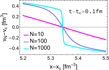
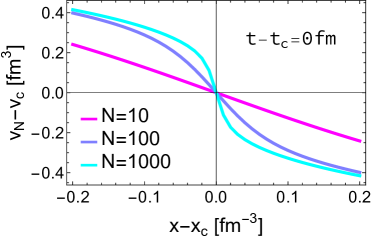
Figure 1: Universal behavior and finite-size corrections in the vicinity of QCD critical points at $t-t_{c}=0.1$ fm (left) and $t-t_{c}=0$ fm (right). The parameters are chosen from Eq. (22) for the QCD critical point.

Finding the generalized Burgers equation (18) enables to argue on the expected modifications to the fluid EOS when $N$ is finite in terms of a well-posed mathematical problem. In particular, it is well understood that the $1/N$ viscous term in Eq. (18) prevents the appearance of singular behavior at the critical points that would originate in the “inviscid limit” at $N\to\infty$. Besides, fundamental results can be adapted in respect to the approaching to the critical region. More precisely, a connection is established with a remarkable mathematical result known in the theory of integrable systems as Universality Conjecture dubrovin2006 ; dubrovin2012 . Following dubrovin2012 , we are therefore led to deduce that near a given critical point located at $t_{c},x_{c},{\rm v}_{c}$, the solution to Eq. (18) behaves as

$${\rm v}_{N}(t,x)={\rm v}_{c}+\frac{\gamma}{N^{\frac{1}{4}}}\,U\left(\frac{\Delta x+\epsilon^{\prime}({\rm v}_{c})\Delta t}{\alpha N^{-\frac{3}{4}}},\frac{\Delta t}{\beta N^{-\frac{1}{4}}}\right)\\ +O(N^{-\frac{1}{2}})$$ (19)

where $\Delta x=x-x_{c}$, $\Delta t=t-t_{c}$, and the function $U(r_{1},r_{2})$ is defined via logarithmic derivative of the Pearcey function:

$$U(r_{1},r_{2})=-2\partial_{r_{1}}\ln\int^{\infty}_{-\infty}dre^{-\frac{1}{8}(r^{4}-2r^{2}r_{2}+4rr_{1})}\,.$$ (20)

The scale parameters in Eq. (19) are specified via $\alpha=\frac{1}{2\gamma}=(\frac{\kappa}{8})^{1/4},\beta=(\frac{\kappa}{2[\epsilon^{\prime\prime}({\rm v}_{c})]^{2}})^{1/2}$, where $\kappa=\frac{1}{6}\left[\epsilon^{(4)}({\rm v}_{c})\,t_{c}-s^{(4)}({\rm v}_{c})\right]$. The “critical EOS” (19) at various values of $N$ is shown in Fig. 1, illustrating how the critical signature smooths out at small $N$.

Example: Phase transitions in QCD—An important example of a physical system displaying multiple critical points is represented by nuclear matter whose underlying physics is described by QCD Stephanov:2006zvm . The two major properties of quarks and gluons, i.e., asymptotic freedom at high energy and confinement at low energy, indicate two different phases separated by a first-order phase transition (FOPT): the quark-gluon plasma (QGP) and hadron gas (HG) Sorensen:2023zkk . The latter also features a vdW-type nuclear L-G transition at low energy due to hadronic interactions PhysRevLett.75.1040 ; Wang:2020tgb . Effective mean-field models for describing both critical points are feasible by choosing baryon density $n_{B}$ as the order parameter which is well defined across different QCD scales. Indeed, it has been emphasized that mean-field statistical mechanics approaches to QCD matter prove to be very effective because they naturally lead to EOS reproducing the known properties of ordinary nuclear matter, and they allow to explore critical behavior in dense nuclear matter over vast regions of the QCD phase diagram SorensenPhysRevC.104.034904 ; PhysRevLett.131.202303 .

quantity	value	quantity	value
$T_{c,1}$	0.10 fm-1	$T_{c,2}$	0.51 fm-1
${\rm v}_{c,1}$	16.45 fm3	${\rm v}_{c,2}$	2.08 fm3
${\rm v}_{a}$	2.40 fm3	${\rm v}_{b}$	1.89 fm3

Table 1: Physical values chosen to determine coefficients in Eq. (22).

In the isothermal–isobaric ensemble, the order parameter is the volume density ${\rm v}=1/n_{B}$. We therefore propose a phenomenological mean-field model by assuming that the phase transitions governed by QCD can be described by such order parameter via the hard-sphere entropy and potential energy (9), taking a virial-type expansion with $m=6$. Accordingly, in the $N\to\infty$ limit, Eq. (15) implies the following EOS

$$P({\rm v},T)=\frac{T}{{\rm v}-b}-\sum_{j=2}^{6}\frac{a_{j}}{{\rm v}^{j}}\,.$$ (21)

To determine the parameters $b$ and $a$’s, six independent conditions must be imposed. First, the application of Eq. (16) requires $\partial_{v}P({\rm v}_{c,l},T_{c,l})=\partial_{\rm v}^{2}P({\rm v}_{c,l},T_{c,l})=0$ for the nuclear L-G and HG-QGP transition labeled by $l=1,2$ respectively. The critical volume densities are set to ${\rm v}_{c,1}\simeq 1/(0.38n_{0})$ at $T_{c,1}=20~\text{MeV}\simeq 0.10~\text{fm}^{-1}$ and ${\rm v}_{c,2}\simeq 1/(3n_{0})$ at $T_{c,2}=100~\text{MeV}\simeq 0.51~\text{fm}^{-1}$, where $n_{0}\simeq 0.16/\text{fm}^{3}$ is the nuclear saturation density Fukushima_2011 . Furthermore, at $T=0$ MeV, the two spinodal points for the HG-QGP transition are located at ${\rm v}_{a}=1/(2.6n_{0})$ and ${\rm v}_{b}=1/(3.3n_{0})$, with $\partial_{\rm v}P({\rm v}_{a},0)=\partial_{\rm v}P({\rm v}_{b},0)=0$. From the above six conditions, whose explicit values are listed in Table 1, one obtains

$$a_{2}\! \simeq 16{\rm v}_{0}\,\text{MeV},\,a_{3}\!\simeq 108{\rm v}_{0}^{2}\,\text{MeV},\,a_{4}\!\simeq\!\!-213{\rm v}_{0}^{3}\,\text{MeV},$$

$$a_{5}\! \simeq 93{\rm v}_{0}^{4}\,\text{MeV},\,a_{6}\!\simeq\!\!-12{\rm v}_{0}^{5}\,\text{MeV},\,b\!\simeq 0.075{\rm v}_{0},$$ (22)

where the saturation volume ${\rm v}_{0}=1/n_{0}$. The resulting isothermal curves of the EOS (21), in the low- and high-volume density regime, are displayed in Fig. 2.

The QCD phase diagram in $T-P$ plane and its remnant at finite $N$ are shown in Fig. 3. While sharp thermodynamic singularities and phase boundaries are well-defined in TL, only their remnants, identified by the locations of the maxima of thermodynamic gradients (e.g., isothermal compressibility or specific heat) persist at finite $N$. As a result, the critical behavior is smoothed out: the singularity at the critical point is smeared, and the TL coexistence curve also turns into a crossover – a remnant of the discontinuity whose location shifts in the phase diagram relative to its position in TL. Our approach extends crossover lines in TL to finite $N$ and shows that different criteria yield notably distinct predictions when finite size corrections are taken into account, in contrast to the TL case, where the predictions are indistinguishable near the critical point doi:10.1073/pnas.0507870102 . We also observed that, at finite size, the shift of the Widom lines determined by the maximum of specific heat is smaller than that from isothermal compressibility, suggesting it as a more accurate estimate of the crossover line in TL limit (see right panel of Fig. 3).

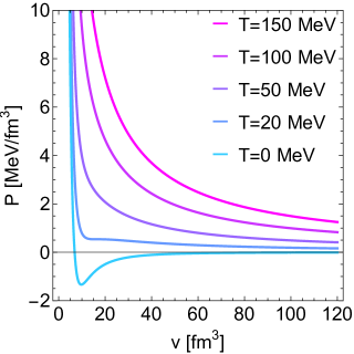
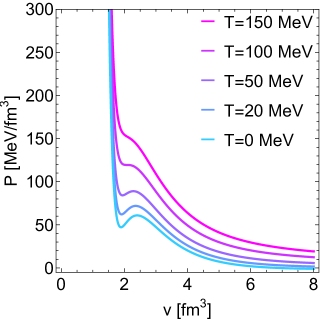
Figure 2: Isothermal curves predicted by the EOS (21) with parameters (22) at different thermodynamic scales. The left and right panels show the nuclear L-G and the HG-QGP transitions, respectively.

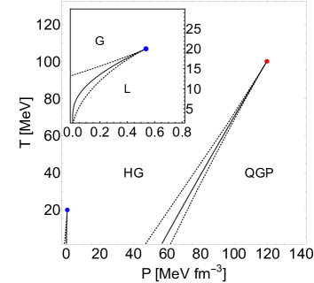
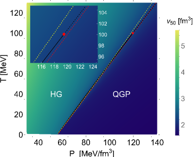
Figure 3: Left: QCD phase diagram in $T-P$ plane, predicted by EOS (21). The blue and red circles represent the nuclear L-G and HG-QGP critical points, respectively, each associated with its corresponding coexistence line (solid) and spinodal lines (dashed). Right: volume density at finite size around the HG-QGP transition region. The loci of maxima of specific heat (dashed red) and isothermal compressibility (dashed yellow) at $N=50$, together with the coexistence (solid black) and cross-over (dashed black) lines in TL are displayed.

Conclusions—We have developed a framework for discussing fluid systems whose internal energy can be written in the virial-type form (3). In particular, we have determined a linear PDE for the partition function, and C-integrable PDEs for the free energy and order parameter (volume density in the isothermal–isobaric ensemble). Gradient catastrophe phenomena and singular solution behaviors, implying discontinuous phase transitions, are allowed in TL $N\to\infty$. Remarkably, phase transitions with discontinuities are instead prevented when finite $N$ leading corrections are retained, and a behavior in agreement with the Universality Conjecture (19) is expected in the vicinity of a critical region. Furthermore, our approach leads to prediction of the volume density along the coexistence lines at finite $N$ in terms of the thermodynamic potential around competing phases.

The formalism has then been implemented into the phase behavior of QCD, which remains poorly understood to this day Guenther:2020jwe . Our findings on finite-size effects lead to the conclusion that the search for the QCD critical point in experiments might be even more challenging than figured insofar. Indeed, these effects, varying with the system size, may obscure key characteristic signatures such as the enhanced fluctuations of conserved quantities. Consequently, interpreting experimental data, including those from RHIC Beam Energy Scan program STAR:2020tga and NA61/SHINE experiments Adhikary:2023rfj , requires careful consideration of finite-size effects to ensure reliable conclusions.

Our results can be complemented by extending the formalism to ensembles described by different thermodynamic variables, such as chemical potentials and magnetic field, and incorporate our EOS into hydrodynamic simulations as an equilibrium baseline for studying nonequilibrium processes like those occurring in heavy-ion collisions. The consequence of complexity due to fluctuations in effective potential shall also be explored in a finite-size system An:2017brc . We leave these for future work.

- (1) G. Parisi, Nobel lecture: Multiple equilibria, Rev. Mod. Phys. 95 (2023) 030501.
- (2) B.J.İ. Beycan İbrahimoğlu, Critical States at Phase Transitions of Pure Substances, Springer (2022).
- (3) S.Z. Cheng, Phase Transitions in Polymers: The Role of Metastable States, Elsevier (2008).
- (4) A. Pelissetto and E. Vicari, Critical phenomena and renormalization-group theory, Phys. Rep. 368 (2002) 549.
- (5) M. Combescot and C.B. à la Guillaume, Two critical points for an electron-hole system, Phys. Rev. Lett. 44 (1980) 182.
- (6) Sumedha and S. Mukherjee, Emergence of a bicritical end point in the random-crystal-field blume-capel model, Phys. Rev. E 101 (2020) 042125 [1907.06454].
- (7) A. Maritan, M. Cieplak, M.R. Swift, F. Toigo and J.R. Banavar, Random anisotropy Blume-Emery-Griffiths model, Phys. Rev. Lett. 69 (1992) 221.
- (8) F.S. P.G. Debenedetti and G. Zerze, Second critical point in two realistic models of water, Science 369 (2020) 289.
- (9) T.E. Gartner, P.M. Piaggi, R. Car, A.Z. Panagiotopoulos and P.G. Debenedetti, Liquid-liquid transition in water from first principles, Phys. Rev. Lett. 129 (2022) 255702 [2208.13633].
- (10) L. Ferroni, V. Koch and M.B. Pinto, Multiple critical points in effective quark models, Phys. Rev. C 82 (2010) 055205 [1007.4721].
- (11) M. Ferreira, P. Costa and C. Providência, Multiple critical endpoints in magnetized three flavor quark matter, Phys. Rev. D 97 (2018) 014014 [1712.08378].
- (12) A. Moro, Shock dynamics of phase diagrams, Ann. Phys. 343 (2014) 49 [1307.7512].
- (13) A. Barra and A. Moro, Exact solution of the van der Waals model in the critical region, Ann. Phys. 359 (2015) 290 [1412.1951].
- (14) C.N. Yang and T.D. Lee, Statistical theory of equations of state and phase transitions. i. theory of condensation, Phys. Rev. 87 (1952) 404.
- (15) D. Ruelle, Statistical Mechanics, World Scientific, Singapore (1999).
- (16) P. Borrmann, O. Mülken and J. Harting, Classification of phase transitions in small systems, Phys. Rev. Lett. 84 (2000) 3511 [cond-mat/9909184].
- (17) J. Bernhardt, C.S. Fischer, P. Isserstedt and B.-J. Schaefer, Critical endpoint of QCD in a finite volume, Phys. Rev. D 104 (2021) 074035 [2107.05504].
- (18) G. Kovács, P. Kovács, P.M. Lo, K. Redlich and G. Wolf, Sensitivity of finite size effects to the boundary conditions and the vacuum term, Phys. Rev. D 108 (2023) 076010 [2307.10301].
- (19) P. Lorenzoni and A. Moro, Exact analysis of phase transitions in mean-field potts models, Phys. Rev. E 100 (2019) 022103.
- (20) H. Callen, Thermodynamics and an Introduction to Thermostatistics, Wiley, Singapore (1991).
- (21) A. Chamblin, R. Emparan, C. Johnson and R. Myers, Charged AdS black holes and catastrophic holography, Phys. Rev. D 60 (1999) 064018 [hep-th/9902170].
- (22) M. Oertel, M. Hempel, T. Klähn and S. Typel, Equations of state for supernovae and compact stars, Rev. Mod. Phys. 89 (2017) 015007.
- (23) C. Chin, R. Grimm, P. Julienne and E. Tiesinga, Feshbach resonances in ultracold gases, Rev. Mod. Phys. 82 (2010) 1225–1286 [0812.1496].
- (24) J.I. Kapusta and C. Gale, Finite-temperature field theory: Principles and applications, Cambridge Monographs on Mathematical Physics, Cambridge University Press (2011).
- (25) M. Le Bellac, F. Mortessagne and G. Batrouni, Equilibrium and Non-Equilibrium Statistical Thermodynamics, Cambridge University Press (2006).
- (26) G. De Matteis, F. Giglio and A. Moro, Exact equations of state for nematics, Ann. Phys. 396 (2018) 386 [1802.07246].
- (27) F. Calogero, Why are certain nonlinear PDEs both widely applicable and integrable?, in What Is Integrability?, (Berlin), pp. 1–62, Springer (1991).
- (28) G.B.Whitham, Linear and Nonlinear Waves, John Wiley & Sons, Inc. (1973).
- (29) R. Thom, Structural Stability And Morphogenesis, CRC Press (1989).
- (30) F. Giglio, G. Landolfi and A. Moro, Integrable extended van der Waals model, Physica D: Nonlinear Phenomena 333 (2016) 293 [1602.03975].
- (31) A. Bressan, Hyperbolic systems of conservation laws: the one-dimensional Cauchy problem, Oxford University Press, USA (2000).
- (32) B. Dubrovin, On hamiltonian perturbations of hyperbolic systems of conservation laws, ii: Universality of critical behaviour, Comm. Math. Phys. 267 (2006) 117 [math-ph/0510032].
- (33) B. Dubrovin and M. Elaeva, On the critical behavior in nonlinear evolutionary PDEs with small viscosity, Russ. J. Math. Phys. 19 (2012) 449 [1301.7216].
- (34) M. Stephanov, QCD phase diagram: An Overview, PoS LAT2006 (2006) 024 [hep-lat/0701002].
- (35) A. Sorensen et al., Dense nuclear matter equation of state from heavy-ion collisions, Prog. Part. Nucl. Phys. 134 (2024) 104080 [2301.13253].
- (36) J. Pochodzalla, T. Möhlenkamp, T. Rubehn, A. Schüttauf, A. Wörner, E. Zude et al., Probing the nuclear liquid-gas phase transition, Phys. Rev. Lett. 75 (1995) 1040.
- (37) R. Wang, Y.-G. Ma, R. Wada, L.-W. Chen, W.-B. He, H.-L. Liu et al., Nuclear liquid-gas phase transition with machine learning, Phys. Rev. Res. 2 (2020) 043202 [2010.15043].
- (38) A. Sorensen and V. Koch, Phase transitions and critical behavior in hadronic transport with a relativistic density functional equation of state, Phys. Rev. C 104 (2021) 034904 [2011.06635].
- (39) M. Omana Kuttan, J. Steinheimer, K. Zhou and H. Stoecker, QCD equation of state of dense nuclear matter from a bayesian analysis of heavy-ion collision data, Phys. Rev. Lett. 131 (2023) 202303 [2211.11670].
- (40) K. Fukushima and T. Hatsuda, The phase diagram of dense QCD, Rep. Prog. Phys. 74 (2010) 014001 [1005.4814].
- (41) L. Xu, P. Kumar, S.V. Buldyrev, S.-H. Chen, P.H. Poole, F. Sciortino et al., Relation between the widom line and the dynamic crossover in systems with a liquid–liquid phase transition, Proceedings of the National Academy of Sciences 102 (2005) 16558.
- (42) J.N. Guenther, Overview of the QCD phase diagram: Recent progress from the lattice, Eur. Phys. J. A 57 (2021) 136 [2010.15503].
- (43) STAR collaboration, Nonmonotonic Energy Dependence of Net-Proton Number Fluctuations, Phys. Rev. Lett. 126 (2021) 092301 [2001.02852].
- (44) NA61/SHINE collaboration, Search for the QCD critical point by NA61/SHINE at the CERN SPS, in 10th International Conference on New Frontiers in Physics, 8, 2023 [2308.04254].
- (45) X. An, D. Mesterházy and M.A. Stephanov, On spinodal points and Lee-Yang edge singularities, J. Stat. Mech. 1803 (2018) 033207 [1707.06447].