Approximation properties of neural ODEs
Abstract
We study the approximation properties of shallow neural networks whose activation function is defined as the flow of a neural ordinary differential equation (neural ODE) at the final time of the integration interval. We prove the universal approximation property (UAP) of such shallow neural networks in the space of continuous functions. Furthermore, we investigate the approximation properties of shallow neural networks whose parameters are required to satisfy some constraints. In particular, we constrain the Lipschitz constant of the flow of the neural ODE to increase the stability of the shallow neural network, and we restrict the norm of the weight matrices of the linear layers to one to make sure that the restricted expansivity of the flow is not compensated by the increased expansivity of the linear layers. For this setting, we prove approximation bounds that tell us the accuracy to which we can approximate a continuous function with a shallow neural network with such constraints. We prove that the UAP holds if we consider only the constraint on the Lipschitz constant of the flow or the unit norm constraint on the weight matrices of the linear layers.
1 Introduction
Approximation theory is a branch of mathematics concerned with approximating functions with simpler ones and quantitatively characterizing the errors thereby introduced. Approximation is a generalization of representation. Given a space of functions, generally the space of continuous functions from to , fixed, and a subset of continuous functions, we say that
-
•
a function is represented by if ,
-
•
a function is approximated by if for any there exists that is close to up to error , under some topology that will be defined at a later time.
In other words, a function is approximated by if , and we say that is a universal approximator for if is dense in , i.e. . Representation is a very strong requirement that is very difficult to satisfy. Nevertheless, the fact that some continuous functions cannot be represented by some subset does not prevent them from being approximated by .
For example, let us consider the MNIST [1] handwritten digits classification problem. The task is to correctly classify each of its images, i.e., to determine the digit represented by each image. We collect some MNIST images in Figure 1.
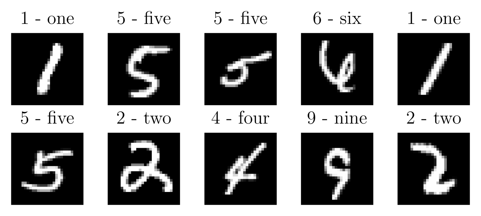
Since each image has resolution , the function that classifies the MNIST images is an unknown function . It is unlikely to be able to represent the function . Nevertheless, we can approximate it by a suitably chosen set of functions , such as neural networks.
Neural networks are parametric maps obtained by composing affine and nonlinear functions. We define a neural network of layers as follows
where is the nonlinear activation function applied entry-wise, whereas the affine functions are defined as
with , , , and . We denote by the width of the neural network and we call its depth. We distinguish two cases:
-
•
if , we call a shallow neural network,
-
•
if , we call a deep neural network.
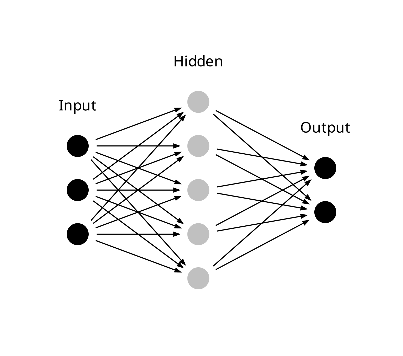
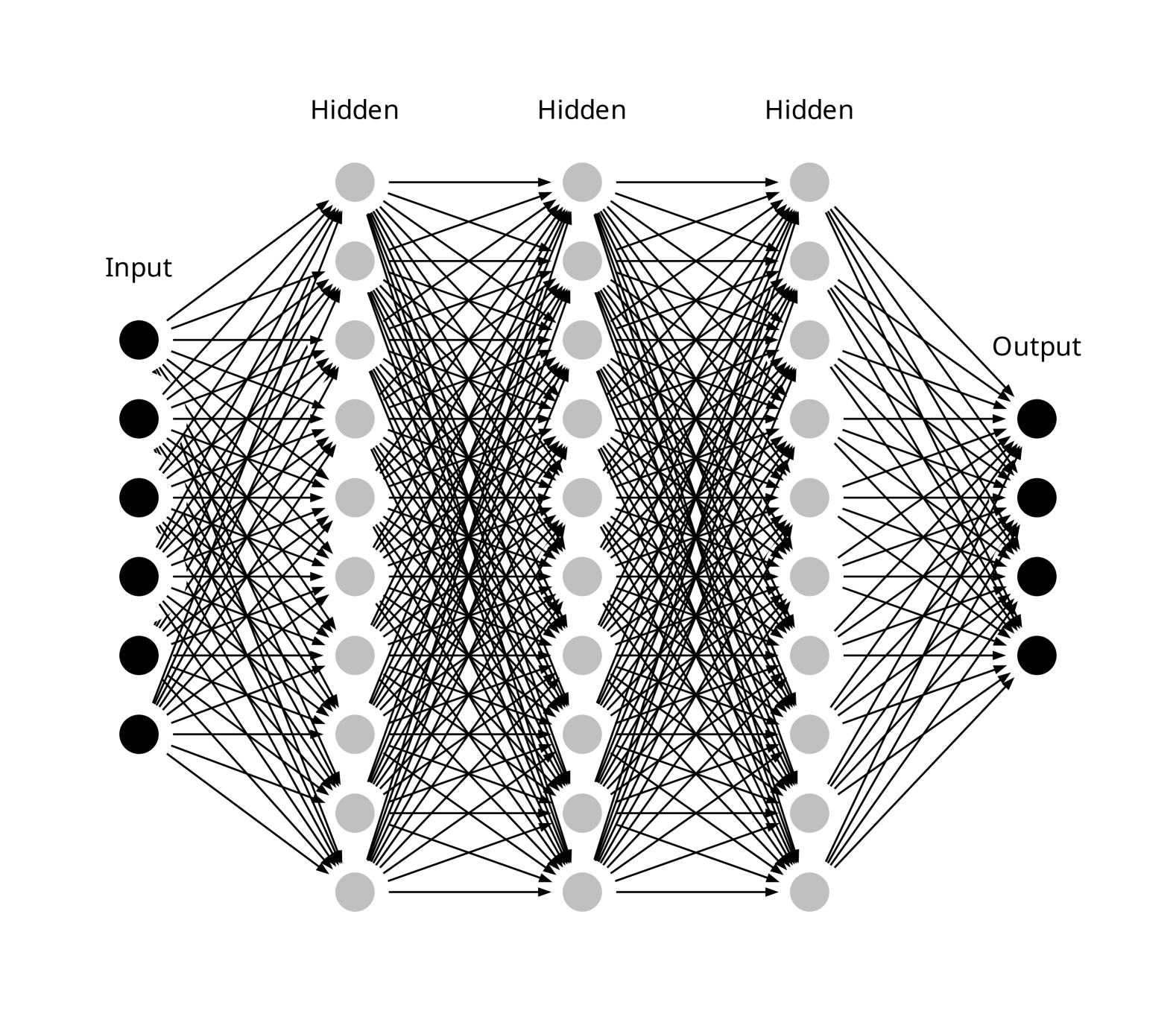
Neural networks have a graphical representation shown in Figure 2. The input and the output layers correspond to the input and to the output respectively, while the -th hidden layer, , corresponds to the input transformed by the first functions that constitute the neural network , i.e. to the quantity .
1.1 Related works
Neural networks are the most common choice of approximators for continuous functions in applications since their approximation capacity has been certified by many studies in the past few decades, and it still is an active research area.
In 1989, Cybenko [2] and Hornik et al. [3] showed that shallow neural networks with arbitrary width and sigmoidal activation functions, i.e., increasing functions with and , are universal approximators for continuous functions. In 1991, Hornik [4] showed that it is not the specific choice of the activation function but rather the compositional nature of the network that gives shallow neural networks with arbitrary width the potential of being universal approximators. In 1993, Leshno et al. [5] and, in 1999, Pinkus [6] showed that shallow neural networks with arbitrary width are universal approximators if and only if their activation function is not a polynomial. Other relevant references for the approximation properties of shallow neural networks with arbitrary width are [7, 8, 9, 10].
The recent breakthrough of deep learning has stimulated much research on the approximation capacity of arbitrarily deep neural networks with bounded width. Gripenberg in 2003 [11], Yarotsky, Lu et al. and Hanin and Selke in 2017 [12, 13, 14] studied the universal approximation property of deep neural networks with arbitrary depth, bounded width, and with ReLU activation functions. Kidger and Lyons in 2020 [15] extended those results to arbitrarily deep neural networks with bounded width and arbitrary activation functions. Park in 2021 [16] improved the results by Hanin [14] for deep ReLU neural networks with bounded width, and Cai [17] in 2023 proved the approximation property for deep neural networks with bounded width and with the LeakyReLU activation function. More details about the approximation of arbitrarily deep ReLU neural networks for continuous functions, smooth functions, piecewise smooth functions, shift invariant spaces and band-limited functions are available in [12, 18, 19], [20, 21], [22], [23] and [24] respectively. Other valuable references for the approximation properties of arbitrarily deep neural networks with bounded width are [25, 26, 27, 28].
In 1999, Maiorov and Pinkus [29] studied the bounded depth and width case. They showed that there exists an analytic sigmoidal activation function such that neural networks with two hidden layers and bounded width are universal approximators. In 2018, Guliyev and Ismailov [30] designed a smooth sigmoidal activation function such that two hidden layer feed-forward neural networks with such activation function are universal approximators with smaller width. In the same year, Guliyev and Ismailov [31] also constructed shallow neural networks with bounded width that are universal approximators for univariate functions. However, this construction does not apply to multivariate functions. In 2022, Shen et al. [32] computed precise quantitative information on the depth and width required to approximate a target function by deep and wide ReLU neural networks.
1.2 Our contribution
In this paper, we study the approximation properties of shallow neural networks of arbitrary width and with an activation function given by the flow of a neural ODE [33] at time . We consider the compact convergence topology as in [2, 3, 4, 5].
Definition 1.1.
Let and a norm of . A set of functions from to is a universal approximator for under the compact convergence topology if, for any , for any compact, and for any , there exists such that
In Definition 1.1, we leave the norm as an unspecified norm of . Later derivations will focus on the norm . In the following, we define the subspace as the space of shallow neural networks of arbitrary width with an activation function given by the flow of a neural ODE at time .
Let and be an activation function that satisfies the following assumption.
Assumption 1.1.
is differentiable almost everywhere and , with .
Remark 1.1.
An example of such an activation function is the LeakyReLU
or a smoothed version of it, like
| (1) |
where is such that and such that (see Figure 3).
We consider the shallow neural network
| (2) |
with , , , , and the activation function is the time flow of the neural ODE
| (3) |
with , , for all , and is applied entrywise. If we define the affine functions
we can rewrite as follows
i.e., as the composition of three functions: the affine layer , the activation function , and the affine layer .
Remark 1.2.
From here on, when referring to the flow of the neural ODE (3), we always consider it at time .
Before formally introducing the space , we need the following definitions.
Definition 1.2.
Fix . We define the space of affine transformations from to as
Definition 1.3.
Let be the flow of the neural ODE (3) for fixed and . We define the space of neural ODE flows as
where are the weight matrices and the bias vectors.
Then we can define the subspace of as follows.
Definition 1.4.
We define the space of shallow neural networks (2) from to with activation function defined as a neural ODE flow as
1.3 Paper organization
The paper is organized as follows. In Section 2, it is proved that the space of shallow neural networks of arbitrary width, with the proposed choice of activation function, is a universal approximator for the space of continuous functions under the compact convergence topology. The section ends by introducing two constraints that improve the stability of the proposed shallow neural network at the risk of losing the universal approximation property. The former is a constraint on the Lipschitz constant of the activation function to restrict its expansivity, the latter is a constraint of unit 2-norm of the weight matrices and to make sure the restricted expansivity of the activation function is not compensated by the increased expansivity in the linear layers. Section 3 is dedicated to deriving approximation bounds that tell us how accurately we can approximate a continuous function with a shallow neural network with both constraints. In Section 4, the universal approximation property is shown to hold if only the constraint on the Lipschitz constant of the activation function or the unit norm constraint on the weight matrices of the linear layers is considered.
2 Universal approximation theorem
We are ready to state the first main result of this paper.
Theorem 2.1.
The space of functions
is a universal approximator for under the compact convergence topology.
To prove Theorem 2.1, we need the following definition and lemmas.
Definition 2.1.
Let denote the set of real functions which are in and have the following property: the closure of their sets of points of discontinuity is of zero Lebesgue measure.
For each function , interval , and scalar , there exists a finite number of open intervals, the union of which we denote by , of measure , such that is uniformly continuous on . This is important in the proof of the next lemma.
Lemma 2.1 (Theorem 1, page 10, [5]).
Let . Set
Then is dense in under the compact convergence topology if and only if is not a polynomial.
Lemma 2.1 is the first universal approximation theorem by Leshno et al. [5] stating a very simple condition for the space of shallow neural networks to be a universal approximator for , i.e. the activation function has not to be a polynomial. All commonly used activation functions, such as ReLU, LeakyReLU, and , satisfy this requirement.
Remark 2.1.
Lemma 2.1 implies the universal approximation property of the space of functions
in . Indeed, if
with applied entrywise,
, and , , and , then the -th component of is
We notice that for all , and since is dense in under the compact convergence topology if is not a polynomial, then is dense in under the same topology.
The important hypotheses to remember here are that the activation function is applied entrywise and that it is not a polynomial.
The next Lemma follows.
Lemma 2.2 (Proposition 4.2, page 179 in [34]).
Let , , be a real polynomial flow in for all times , and , the corresponding differential equation, i.e., . Then there are constants such that and
where we interpret to be for .
Lemma 2.2 states that the only scalar differential equations whose flow is a polynomial in are the linear differential equations, and their flow is a linear polynomial in . This is crucial for the proof of Theorem 2.1.
Proof of Theorem 2.1.
Let us consider the time flow , , of the differential equation
| (4) |
with satisfying Assumption 1.1 and the vector of all ones. Assumption 1.1 guarantees that is Lipschitz continuous and thus the existence and uniqueness of the solution of (4). This is a particular case of neural ODE (3) with the identity matrix and a vector with coinciding entries. Written componentwise, (4) turns into the scalar uncoupled ODEs
Therefore all the components of the flow map coincide, i.e., , with for all .
We define the space
of flows of the differential equations (4), and the space
| (5) |
A generic function of has the form
with , , and . Since has components all equal, it can be interpreted as a scalar univariate activation function applied entrywise, that is the time–1 flow of the scalar differential equation
Therefore, since is not a polynomial for Lemma 2.2, Lemma 2.1 holds and is a universal approximator for under the compact convergence topology.
Finally, since , it follows for transitivity that is a universal approximator for under the compact convergence topology. ∎
Remark 2.2.
Theorem 2.1 shows the universal approximation property of shallow neural networks whose activation function is defined as the flow of neural ODE (3). To the best of our knowledge, such activation functions have not been considered so far.
Before we continue, we need the definition of logarithmic norm.
Definition 2.2 (see [35, 36]).
Given and a matrix , denoted by a matrix norm induced by a vector norm, we define the logarithmic norm of as
Remark 2.3.
If the matrix norm is induced by the 2-norm , then the logarithmic 2-norm of , denoted by , coincides with the largest eigenvalue of its symmetric part .
We point out that there are two main differences between flows of neural ODEs (3) and classical activation functions.
- •
-
•
Classical activation functions are 1-Lipschitz functions, while flows of neural ODEs (3) are Lipschitz functions but their Lipschitz constant depends on the weight matrix . In particular, in [37, 38] it has been shown that the Lipschitz constant of the flow of the neural ODE (3) is bounded by
(6) where is defined in Assumption 1.1 and
(7)
2.1 Remarks on stability
The bound on the Lipschitz constant (6) allows us to state the following stability bound for the shallow neural network (2): if are two inputs, then
| (8) | ||||
i.e. a perturbation in input is amplified at most by a factor in output. This information is very useful in light of the fragility of neural networks to adversarial attacks [39, 40, 41], perturbations in input designed to make the neural network return a wrong output, and it suggests an approach to improve the stability of the model (2).
If we set , then the only term that controls the stability of the shallow neural network (2) is . In [37], an efficient numerical method has been proposed to compute , and therefore . Let us denote
For shallow neural networks as in (2) trained using stochastic gradient descent, we experimentally notice that unconstrained neural ODEs tend to have , and thus they are intrinsically unstable. For example, back to the MNIST classification problem (see Figure 1), a shallow neural network of the kind (2) trained to correctly classify the images in the dataset has accuracy777The accuracy is the percentage of correctly classified images in the test set. of and has a constant . See [38, Section 5] for more details on this numerical experiment. Having a constant implies that the Lipschitz constant of the shallow neural network is at most , which is very high and allows some perturbations in input to change the output drastically. Figure 4 shows the accuracy of the shallow neural network as a function of the magnitude of the perturbation introduced in input. The considered perturbation is the FGSM (Fast Gradient Sign Method) adversarial attack [39, 40, 41].
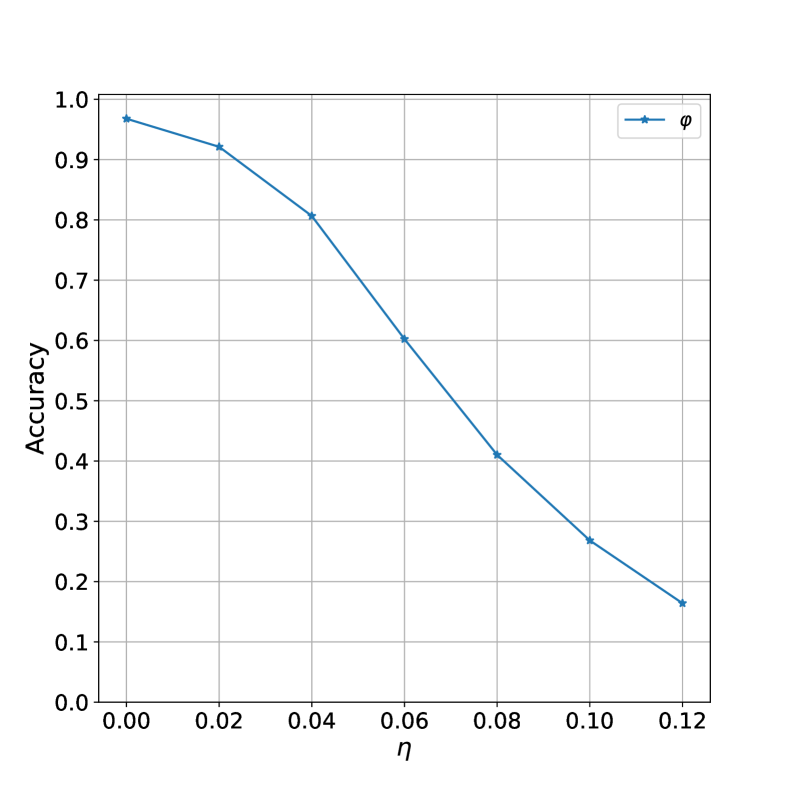
We notice that the accuracy decays quickly as the magnitude of the perturbation increases.
Therefore, in [38], a numerical approach has been proposed to stabilize the shallow neural network . It is sketched as follows. For a fixed , the numerical method computes one of the perturbations with smallest Frobenius norm such that
We say “one of the perturbations” because the underlying optimization problem is not convex, see [37, Remark 5.1]. We have the following scenarios. The shallow neural network (2) is
-
•
slightly expansive if but not large, i.e., but not large;
-
•
nonexpansive if , i.e., ;
-
•
contractive if , i.e., .
Therefore, choosing a close to zero and applying the numerical method proposed in [38] to get allows us to get a shallow neural network of the kind (2) that is at most moderately expansive, i.e. stable. In particular, if
is the stabilized neural ODE and is its time–1 flow, then the stabilized shallow neural network is
| (9) |
Nevertheless, this approach poses two important questions.
-
(a)
Can we quantify the performance variation resulting from the inclusion of the perturbation in the model (2)?
-
(b)
Does adding the constraint or limiting the Lipschitz constant of the flow affect the universal approximation property of the shallow neural network (2)?
These two questions motivate the following sections.
3 Approximation bounds
In this Section, we provide an answer to question (a):
-
(a)
Can we quantify the performance variation resulting from the inclusion of the perturbation in the model (2)?
In this section, we investigate the approximation properties of neural networks with a constrained Lipschitz constant. We focus on the flow . However, to ensure its restricted expansivity is not compensated by the increased expansivity in the linear layers, we limit the norm of the matrices and to one. We introduce the following space.
Definition 3.1.
Fix . We define the space of unit norm affine transformations from to as
We then focus on the space of neural networks defined by
Recall that is the space of shallow neural networks (2) with unit norm constraints on the weight matrices () and activation function defined as the flow of neural ODE (3). We also notice that corresponds to with and instead of and .
We recall that the Lipschitz constant of the flow of neural ODE (3) satisfies the bound
Furthermore, if needed, fixed , it is possible to compute one of the perturbation matrices of minimal Frobenius norm such that (see [37, Remark 5.1],[38]), i.e., the Lipschitz constant of the flow of neural ODE , , is such that
Without constraints of any kind, the Lipschitz constant of the shallow neural network (2) satisfies the bound
If we impose the Lipschitz constant of the flow of the neural ODE (3) to be smaller or equal than for a certain , and we restrict the norm of the matrices and to one, then we lose the universal approximation property. For example, if we aim to approximate a function that is Lipschitz, say , with a shallow neural network (2) with Lipschitz constant bounded by 5, we fail to approximate it arbitrarily well. Nevertheless, we can consider the following questions.
-
(c)
How much does the approximation accuracy degrade because of the perturbation matrix ?
-
(d)
Is there a lower bound on how accurately we can approximate a target function with such a restricted neural ODE?
If we define the approximation error on a compact subset of between a continuous function and a shallow neural network , see (2), as
| (10) |
then the first question leads to finding an upper bound to (10), whereas the second brings to a lower bound. We need the following lemmas. Their proofs are well-known but we write them for completeness in Appendix A.
3.1 Preliminaries
Lemma 3.1.
Given , let us consider the linear scalar differential inequality
with and . Then
Remark 3.1.
An analogous version of Lemma 3.1 holds with instead of .
Lemma 3.2.
If , with , and , then
where, from here on, and denote the largest and the smallest singular values of a matrix respectively.
Lemma 3.3.
If , with , and , then
Furthermore, we consider the time flows and , , where and . To simplify the notation, we define and .
-
•
is the solution of the initial value problem
(11) -
•
is the solution of the initial value problem
(12)
We are ready to state the main results of this section.
3.2 Approximation upper bound
Theorem 3.1.
Given a function , a compact subset of , and a shallow neural network such that
for some , we define . For a fixed , there exists a perturbation matrix such that
Define
Then there exist such that
Proof.
We recall that
For a fixed , by the triangle inequality, we get
so we need to estimate . By definition of and , we have that
| (13) | ||||
since . Therefore, we need to estimate the difference of the flows of two differential equations from the same initial datum.
We define and for all as in (11) and (12), with and . Then, for , we compute
| (14) | ||||
where in the second equality we have used the first order Taylor expansion of and of and in the last equality we have used the expressions of the derivatives given by the differential equations (11) and (12). We omit from here on the dependence on , and we focus on the term . Lagrange Theorem ensures the existence of , a point on the segment joining and , such that
where is the Jacobian matrix of evaluated at , denoted by . We notice that . Since , we have that
| (15) | ||||
Therefore, using (15), Lemma 3.2, and the triangle inequality, we get that
We recall that and that by definition of , and we define , with . Notice that depends on the fixed and, when clear, we omit the argument . Then
with the largest singular value of . Applying Lemma 3.1 with , , yields
since (see (11) and (12)). In particular, if , we have that
| (16) |
By plugging (16) into (13), we obtain that
If we define , then
which concludes the proof. ∎
We notice that the proposed upper bound is pointwise in the space of functions, in the sense that it depends on the choice of . Specifically, given a function and a shallow neural network that approximates within the target function , the upper bound depends on the value and the perturbation matrix .
-
•
is the upper bound to the Lipschitz constant of the stabilized shallow neural network .
-
•
is the perturbation computed to define the stabilized shallow neural network . The larger is , the larger is the upper bound, and thus the worse the approximation error may be.
Remark 3.2.
The result above does not necessarily imply that a Lipschitz-constrained neural network cannot accurately approximate any given target function. It simply tells us that if we start from a trained, unconstrained neural network and correct its weights as illustrated above, we can expect a controlled drop in accuracy.
Corollary 3.1.
With the same notations and under the assumptions of Theorem 3.1, if , i.e. is a nonexpansive shallow neural network, then the approximation upper bound becomes
We now move to the approximation lower bound.
3.3 Approximation lower bound
Definition 3.2.
If and are real vectors, the cosine of the angle between the vectors and is defined as
Theorem 3.2.
Given a function , a compact subset of , and a shallow neural network such that
for some , we define . For a fixed , there exists a perturbation such that
We define
and we assume that, fixed , for all
| (17) |
and that the cosine is well defined. Then, there exists and such that
Proof.
We recall that
For a fixed , by the reverse triangle inequality, we get
so we need to compute a lower bound for . Then, by definition of and , and using Lemma 3.2, we have that
| (18) | ||||
with the smallest singular value of . Therefore we need to compute a lower bound for the difference of the flows of two differential equations from the same initial datum.
We define and for all as in (11) and (12), with and . By Assumption (17), it holds that for all . Then, omitting the dependence on and using (15) and Lemma 3.3, we have that
where denotes the angle between and . We recall that and we define . Notice that depends on the fixed and, when clear, we omit the argument . Thus, we get that
| (19) |
Since and , then by assumption (17). Thus, applying Lemma 3.2 and using the fact that , we obtain that
and then
where , with . Notice that depends on the fixed and, when clear, we omit the argument . Applying Lemma 3.1 with , , and , yields
In particular, if , we have that
| (20) | ||||
By plugging (20) into (18), we obtain that
If we define
then
and so
which concludes the proof. ∎
Remark 3.3.
How would the proof of the approximation lower bound change if
Then
and, since,
it follows from Equation (19) that
where . By following the same reasoning of the proof of the approximation lower bound, if we define and , we obtain that
However here, so the approximation lower bound could be negative and therefore useless.
Remark 3.4.
The presented approximation bounds are valid if the shallow neural networks (2) and (9) have the same parameters . However, back to the MNIST classification problem (see Figure 1), if we further train the parameters of
keeping the activation function fixed and fulfilling the constraint and , we obtain the shallow neural network
with and , that is more accurate than . See (2), (3), and (9) for the notations. Indeed, the two models have the same Lipschitz constant since has not changed, but has better accuracy as shown in Table 1. This indicates that the corrected neural ODE with flow is not necessarily the best neural ODE with Lipschitz constant . This does not contradict the result presented above, but it suggests that approximation bounds can be improved by allowing the parameters to change.
| accuracy of | 0.4920 | 0.4543 | 0.7499 |
|---|---|---|---|
| accuracy of | 0.7775 | 0.9035 | 0.9514 |
Remark 3.5.
Not only the shallow neural network has accuracy approaching the accuracy of as approaches , see Table 1, but it is more stable as expected. Back to the MNIST classification problem, Figure 5 shows how the accuracy of and , for , decays as the magnitude of the FGSM adversarial attack perturbation increases. The values of the accuracy are reported in Table 2. See [38, Section 5] for more details.
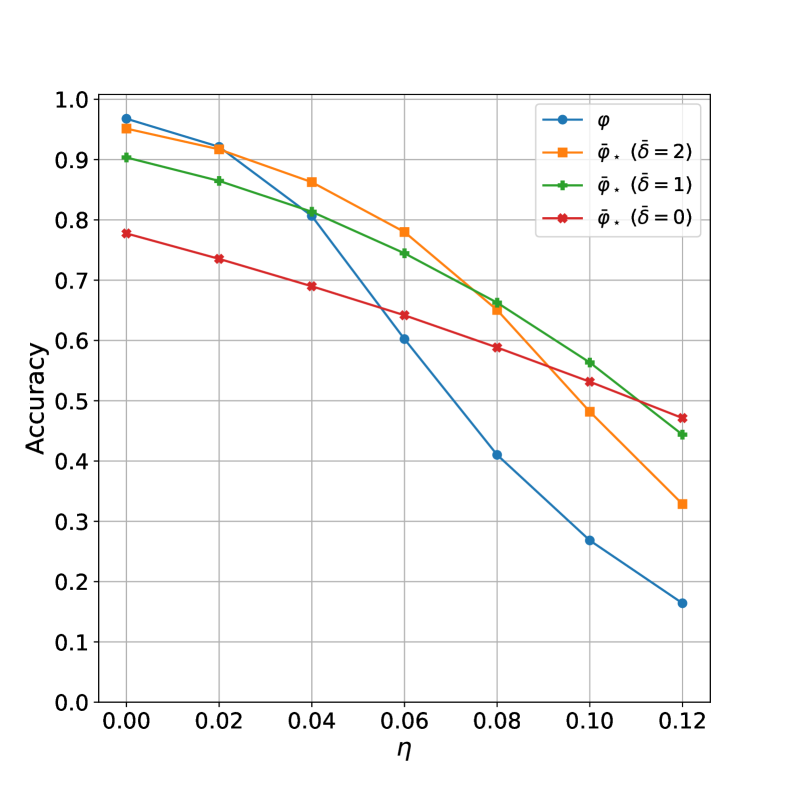
| 0 | 0.02 | 0.04 | 0.06 | 0.08 | 0.10 | 0.12 | |
|---|---|---|---|---|---|---|---|
| 0.9678 | 0.9212 | 0.8065 | 0.6023 | 0.4102 | 0.2683 | 0.1641 | |
| () | 0.9514 | 0.9170 | 0.8626 | 0.7799 | 0.6505 | 0.4818 | 0.3286 |
| () | 0.9035 | 0.8646 | 0.8135 | 0.7446 | 0.6627 | 0.5634 | 0.4437 |
| () | 0.7775 | 0.7353 | 0.6899 | 0.6418 | 0.5883 | 0.5315 | 0.4713 |
Remark 3.6.
We notice that the approximation lower bound does not hold for any compact set . Indeed, it holds for any compact set such that for all assumption (17) holds, i.e.
On the other hand, given a compact set , such assumption can be used to detect those regions of a compact set where (17), and therefore the lower bound, holds. We clarify this with two illustrative examples.
3.4 Illustrative example 1
We consider the function
where is the flow at time 1 of the neural ODE
We choose to be the LeakyReLU with minimal slope , i.e. , and the randomly drawn parameters and as follows.
-
•
Case 1.
-
•
Case 2.
In this setting,
and, following the approach proposed in [37], it turns out that (see Definition 2.2)
-
•
Case 1. ,
-
•
Case 2. .
Given , we compute the smallest (in Frobenius norm) perturbation matrix as in [38] such that
and we denote by the flow of perturbed neural ODE
We now provide an answer to the following question: where does the lower bound for the approximation error
hold in the domain ? It is sufficient to check where Assumption (17) holds in . In this setting, Assumption (17) is simply
since and .
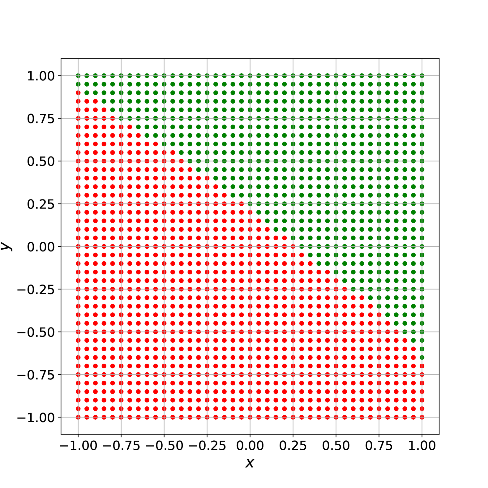
Let us discretize the domain with constant stepsize in both directions and let us call the discretized domain. See Figure 6.
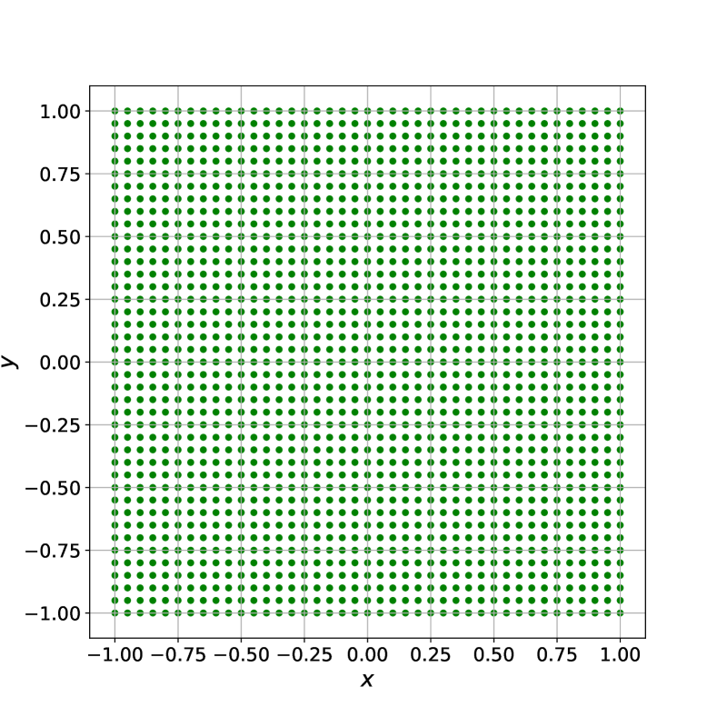
Then, we fix , so that we are safely far from 0, and we introduce a discretization of the time interval with stepsize . We compute for each
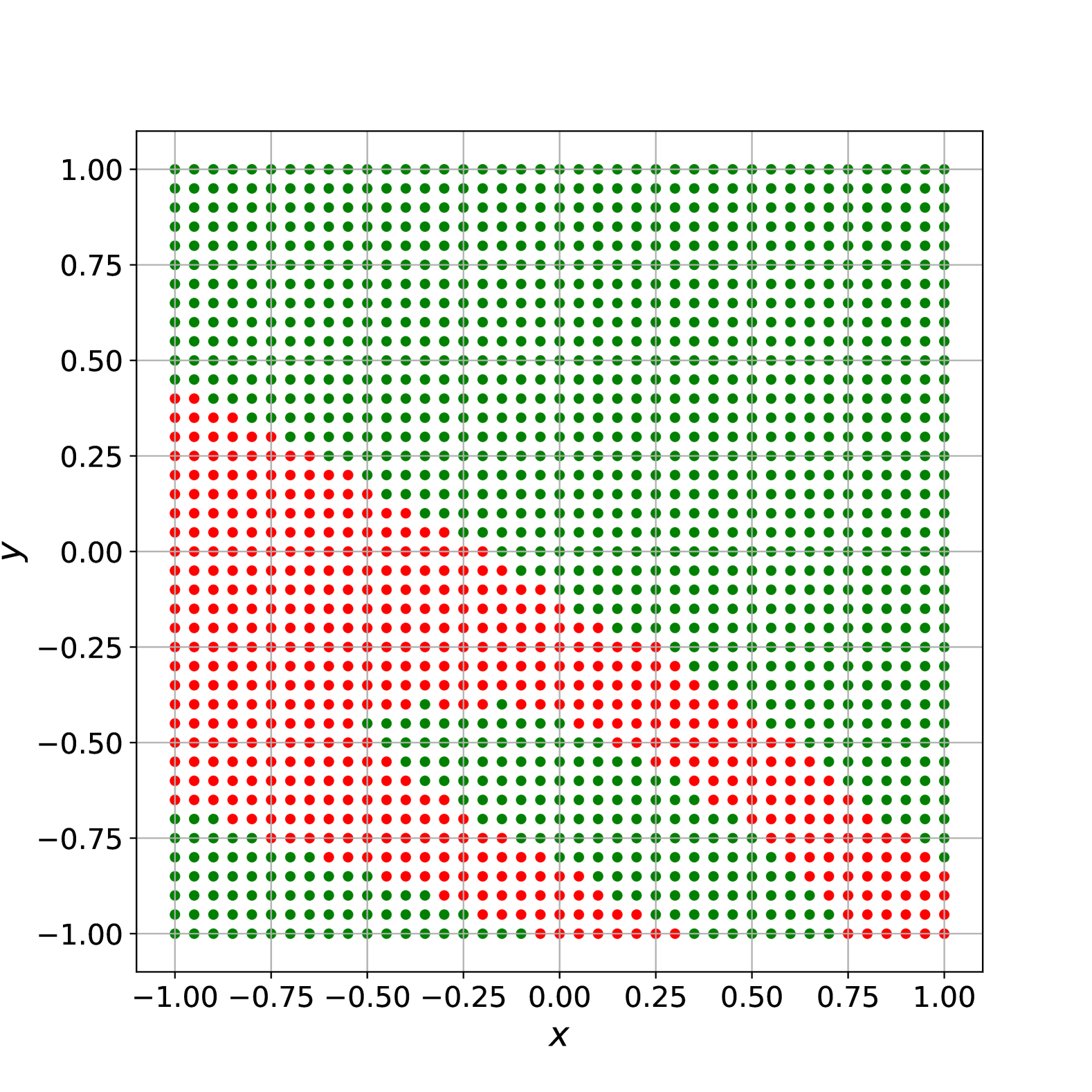
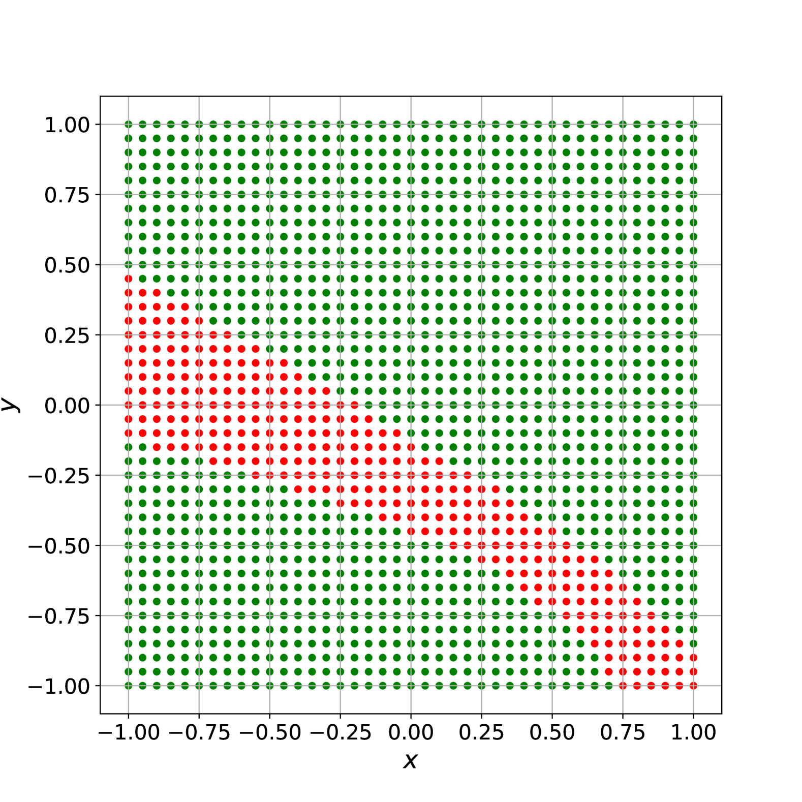
and we leave in green those points for which is positive, while we make red those points for which is negative. We have detected in this way those regions of the discretized domain where the lower bound holds. See Figure 7 for Case 1 and Figure 8 for Case 2. We notice that, as decreases, the green region, where the lower bound holds, expands.
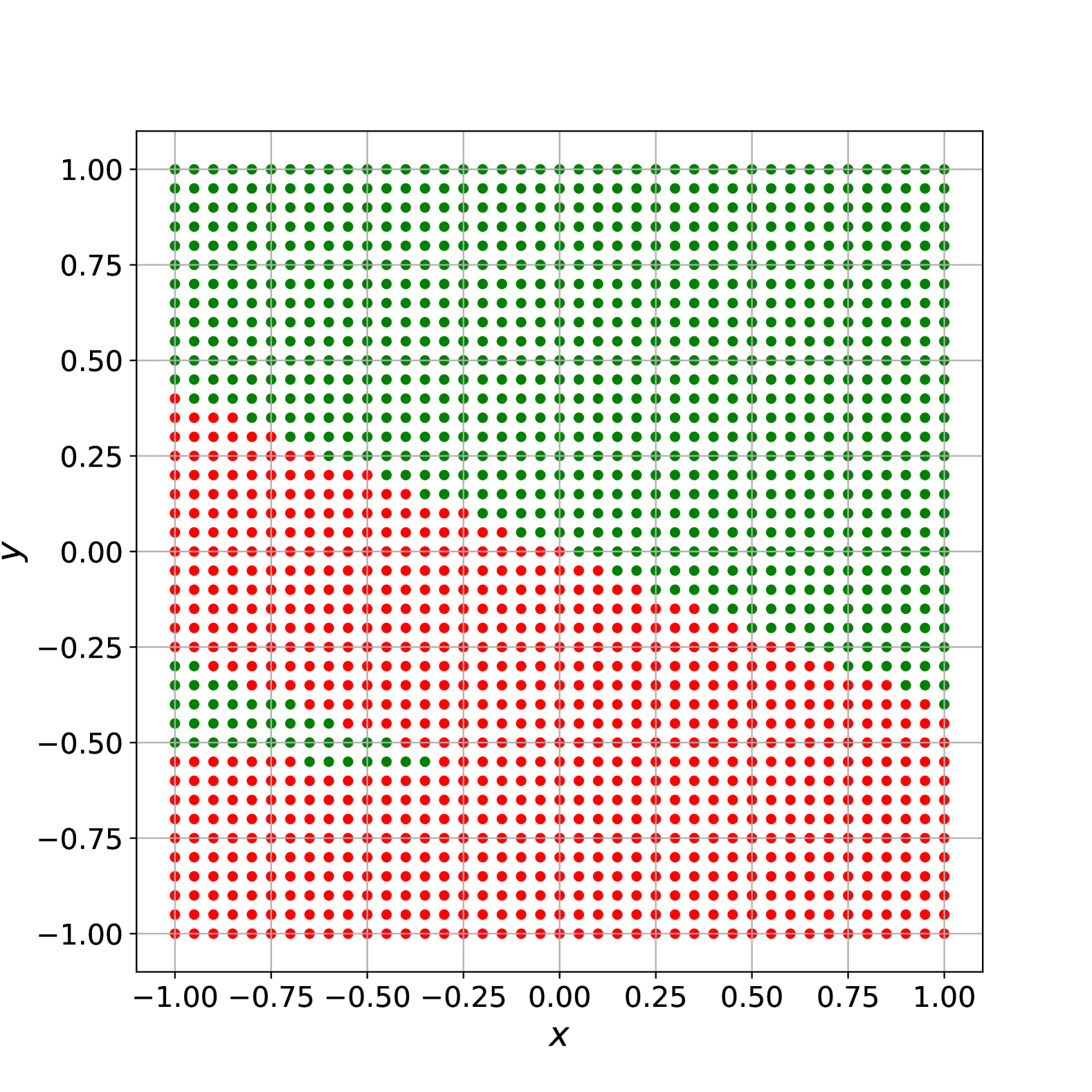

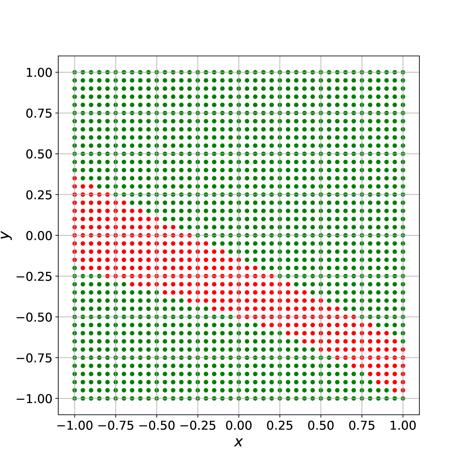
The flows and are computed numerically using the explicit Euler method with constant stepsize 0.05.
3.5 Illustrative example 2
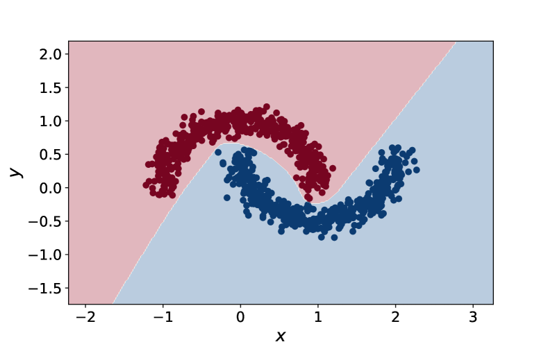
We consider the shallow neural network
where , , , and is the flow at time 1 of the neural ODE
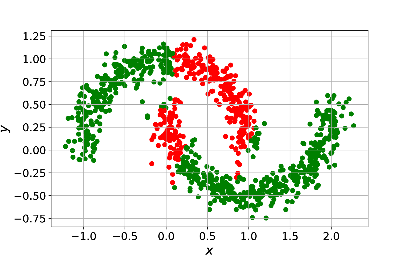
with and . We choose to be the LeakyReLU with minimal slope , i.e. , and we train on the Two Moons dataset. The obtained accuracy is 100%. See Figure 9.
In this setting, has cardinality and, for the trained weight matrix , following the approach proposed in [37], it turns out that (see Definition 2.2)
Given , we compute the smallest (in Frobenius norm) perturbation matrix as in [38] such that
and we denote by the flow of perturbed neural ODE
and by the stabilized shallow neural network
Here the compact subset of interest is the Two Moons dataset itself, and it is already a discrete set. We now provide an answer to the following question: where does the lower bound for the approximation error
hold in the domain ? It is sufficient to check where Assumption (17) holds in . We fix , so that we are safely far from 0, and we introduce a discretization of the time interval with stepsize . We compute for each
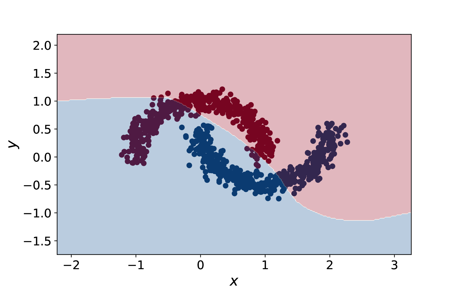
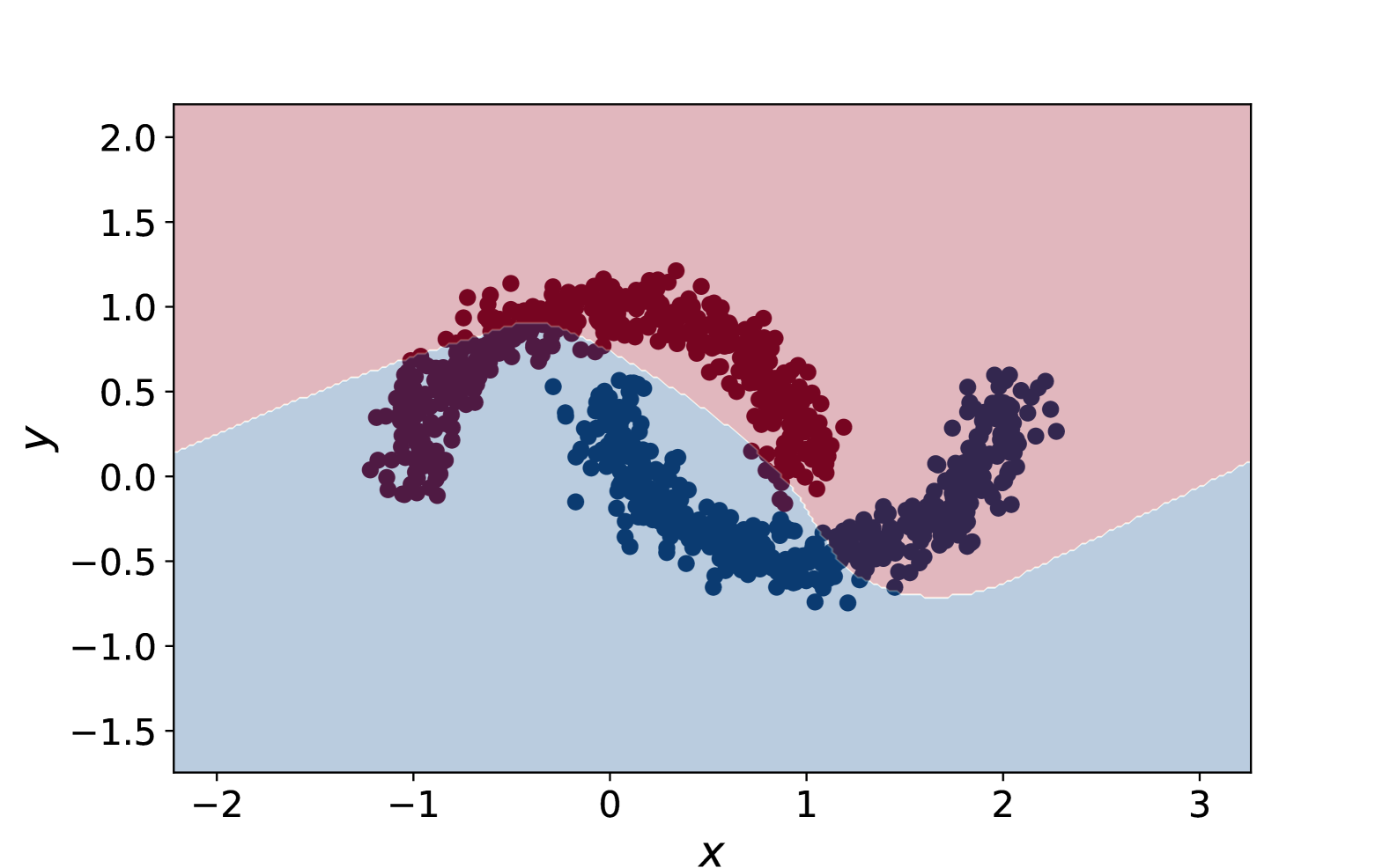
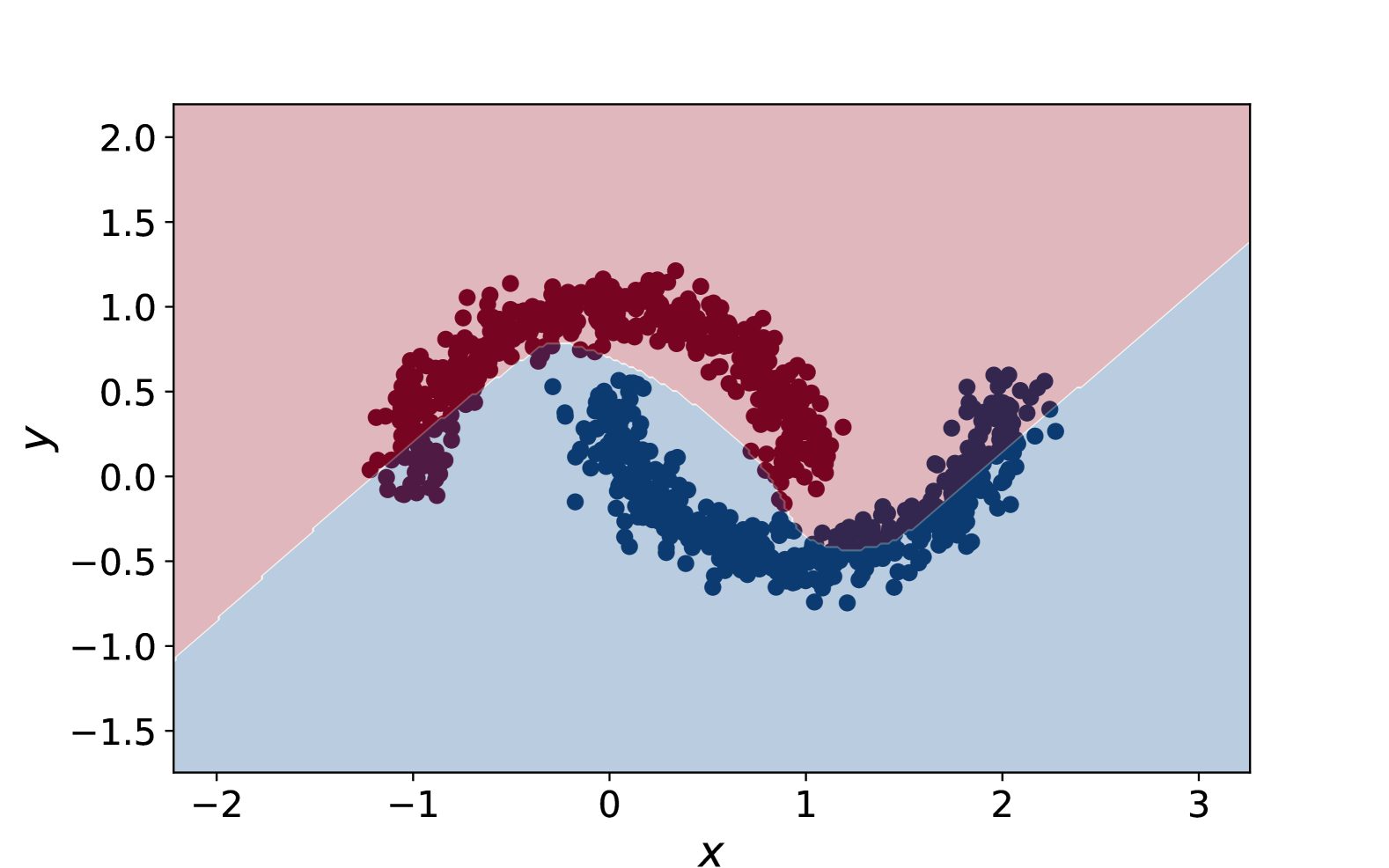
and we make green those points for which is positive, while we make red those points for which is negative. We have detected in this way those regions of the Two Moons dataset where the lower bound holds. See Figure 10 for the green regions where the lower bound holds and Figure 11 for the different classification obtained for the different values of .
We notice that the red region where the lower bound is not guaranteed to hold is the same in the three subfigures of Figure 10. This is consistent with Figure 11 because if the lower bound for the approximation error in the red region does not hold, then and take about the same values in the red region and therefore the stabilized shallow neural network classify the red region correctly.
We also notice that there are regions of the Two Moons dataset where the lower bound holds and that are correctly classified by the stabilized shallow neural network . This happens because we are addressing a classification problem, so and may take different values on the same region and still classify it correctly. Thus, the existence of the lower bound does not prevent the stabilized shallow neural network from correctly classify the points in the region.

4 Universal approximation theorem with Lipschitz constraints
In this Section, we provide an answer to question (b):
-
(b)
Does adding the constraint or limiting the Lipschitz constant of the flow affect the universal approximation property of the shallow neural network (2)?
The intuition tells us that the UAP should hold in both cases. One can think that the restricted expansivity of either the linear layers or the flow could be counteracted by the unconstrained behavior of the other part of the network.
In this case, the Lipschitz constant of is restricted, and formalizing the universal approximation theorem does not require additional work. Indeed, what is important based on Theorem 2.1 is that the flow is not a polynomial. Thus, since there are Lipschitz-constrained non-polynomial flows, the universal approximation property also persists in this constrained regime. As an example, we can think of the differential equation
where , . The Lipschitz constant of its time flow map can be upper bounded by , which can be made equal to any positive number. Thus, since is not linear, the flow is not a polynomial while still being of constrained Lipschitz constant. This proves the universal approximation theorem in this case.
We now move to the case is unconstrained while the weights of the linear layers are of unit spectral norm. Let us recall that the activation function of (2) is the flow of the neural ODE (3), depending on the matrix and the vector . If the matrices and are constrained to have unit 2-norm, then we expect the matrix and the vector to differ from the ones in the unconstrained case, for the flow to have Lipschitz constant larger than the one of the flow in the unconstrained case. In other words, the magnitude of the matrices and can be assimilated in the flow , with a consequent increase of its Lipschitz constant. See (8).
Let us formalize this intuition. We recall that the shallow neural network (2) is
with , , , , and the activation function is the flow of the neural ODE
at time 1, with , , for all and , satisfying Assumption 1.1, is applied entrywise.
We consider the piecewise autonomous neural ODE
| (21) |
where , , each component , , is an autonomous vector field, and is the same vector field of (3). If is an initial datum, then the flow of (21) at is
where is the flow of the neural ODE (3) at time 1. So is essentially a scaled both in the input and in the output, with scaling tuned by and . By choosing the appropriate scaling, the magnitude of the matrices and can be assimilated in the flow, and thus the universal approximation property can be proven also with unit norm weight matrices.
In this section we then work with the shallow neural network
| (22) |
with , , , , and the activation function is the flow of the neural ODE (21), i.e.
We need the following definitions.
Definition 4.1.
Definition 4.2.
We remark that is defined as , where the flow belongs to instead of . We are ready to state the last main result of this paper.
Theorem 4.1.
The space of functions
is a universal approximator for under the compact convergence topology.
Proof.
Let , , and a compact subset of . By Theorem 2.1, there exists such that
By definition of , there exists , and such that
i.e. there exist , , , , , such that
where is the flow of the neural ODE (3). We can rewrite as
with , , and .
Then, we determine and such that
which are
Therefore, there exists a neural ODE (21) with and as above such that its flow is
and .
Eventually, if we define
we have that and and
Therefore also is a universal approximator for under the compact convergence topology. ∎
Remark 4.1.
Introducing neural ODE (21) is only a theoretical expedient to prove the universal approximation property with unit norm constraint on and . A practical reason the implementation of neural ODE (21) is not possible is the lack of knowledge a priori of and . In practise it happens that the Lipschitz constant of the flow of the neural ODE (3) with constrained and is larger than the Lipschitz constant of the flow with unconstrained and . One may think that the magnitudes of and are assimilated by the Lipschitz constant of the flow .
5 Conclusions
We have studied the approximation properties of shallow neural networks whose activation function is defined as the flow of a neural ordinary differential equation (neural ODE) at the final time of the integration interval. We have proved the universal approximation property (UAP) of such shallow neural networks in the space of continuous functions. Furthermore, we have investigated the approximation properties of shallow neural networks whose parameters are required to satisfy some constraints. In particular, we have constrained the Lipschitz constant of the flow of the neural ODE to increase the stability of the shallow neural network, and we have restricted the norm of the weight matrices of the linear layers to one to make sure that the restricted expansivity of the flow is not compensated by the increased expansivity of the linear layers. For this setting, we have proved approximation bounds that tell us the accuracy to which we can approximate a continuous function with a shallow neural network with such constraints. We have eventually proved that the UAP holds if we consider only the constraint on the Lipschitz constant of the flow or the constraint of unit norm of the weight matrices of the linear layers.
Acknowledgements
N.G. acknowledges that his research was supported by funds from the Italian MUR (Ministero dell’Università e della Ricerca) within the PRIN 2022 Project “Advanced numerical methods for time dependent parametric partial differential equations with applications” and the PRO3 joint project entitled “Calcolo scientifico per le scienze naturali, sociali e applicazioni: sviluppo metodologico e tecnologico”. N.G. and F.T. acknowledge support from MUR-PRO3 grant STANDS and PRIN-PNRR grant FIN4GEO. A.D.M., N.G. and F.T. are members of the INdAM-GNCS (Gruppo Nazionale di Calcolo Scientifico). E.C. and B.O. acknowledge that their research was supported by Horizon Europe and MSCA-SE project 101131557 (REMODEL). D.M. acknowledges support from the EPSRC programme grant in “The Mathematics of Deep Learning”, under the project EP/L015684/1, the Department of Mathematical Sciences of NTNU, and the Trond Mohn Foundation for the support during this project.
References
- [1] L. Deng. The MNIST database of handwritten digit images for machine learning research. IEEE Signal Processing Magazine, 29(6):141–142, 2012.
- [2] G. Cybenko. Approximation by superpositions of a sigmoidal function. Mathematics of Control, Signals and Systems, 2(4):303–314, 1989.
- [3] K. Hornik, M. Stinchcombe, and H. White. Multilayer feedforward networks are universal approximators. Neural Networks, 2(5):359–366, 1989.
- [4] K. Hornik. Approximation capabilities of multilayer feedforward networks. Neural Networks, 4(2):251–257, 1991.
- [5] M. Leshno, V. Y. Lin, A. Pinkus, and S. Schocken. Multilayer feedforward networks with a nonpolynomial activation function can approximate any function. Neural Networks, 6(6):861–867, 1993.
- [6] A. Pinkus. Approximation theory of the MLP model in neural networks. Acta Numerica, 8:143–195, 1999.
- [7] K. Funahashi. On the approximate realization of continuous mappings by neural networks. Neural Networks, 2(3):183–192, 1989.
- [8] A. R. Barron. Universal approximation bounds for superpositions of a sigmoidal function. IEEE Transactions on Information theory, 39(3):930–945, 1993.
- [9] M. Hassoun. Fundamentals of Artificial Neural Networks. The MIT Press, 1995.
- [10] S. Haykin. Neural Networks: A Comprehensive Foundation. Prentice Hall, 1998.
- [11] G. Gripenberg. Approximation by neural networks with a bounded number of nodes at each level. Journal of Approximation Theory, 122(2):260–266, 2003.
- [12] D. Yarotsky. Error bounds for approximations with deep ReLU networks. Neural Networks, 94:103–114, 2017.
- [13] Z. Lu, H. Pu, F. Wang, Z. Hu, and Liwei W. The Expressive Power of Neural networks: A View from the Width. In Advances in Neural Information Processing Systems, 2017.
- [14] B. Hanin and M. Sellke. Approximating Continuous Functions by ReLU Nets of Minimal Width. arXiv preprint arXiv:1710.11278, 2017.
- [15] P. Kidger and T. Lyons. Universal Approximation with Deep Narrow Networks. In Conference on Learning Theory, 2020.
- [16] S. Park, C. Yun, J. Lee, and J. Shin. Minimum Width for Universal Approximation. In International Conference on Learning Representations, 2021.
- [17] Y. Cai. Achieve the minimum width of neural networks for universal approximation. In International Conference on Learning Representations, 2023.
- [18] D. Yarotsky. Optimal approximation of continuous functions by very deep ReLU networks. In Conference on Learning Theory, 2018.
- [19] Z. Shen, H. Yang, and S. Zhang. Deep Network Approximation Characterized by Number of Neurons. Communications in Computational Physics, 28(5):1768–1811, 2019.
- [20] D. Yarotsky and A. Zhevnerchuk. The phase diagram of approximation rates for deep neural networks. In Advances in Neural Information Processing Systems, 2020.
- [21] J. Lu, Z. Shen, H. Yang, and S. Zhang. Deep Network Approximation for Smooth Functions. SIAM Journal on Mathematical Analysis, 53(5):5465–5506, 2021.
- [22] P. Petersen and F. Voigtlaender. Optimal approximation of piecewise smooth functions using deep ReLU neural networks. Neural Networks, 108:296–330, 2018.
- [23] Y. Yang, Z. Li, and Y. Wang. Approximation in shift-invariant spaces with deep ReLU neural networks. Neural Networks, 153:269–281, 2022.
- [24] H. Montanelli, H. Yang, and Q. Du. Deep ReLU Networks Overcome the Curse of Dimensionality for Generalized Bandlimited Functions. Journal of Computational Mathematics, 39(6):801–815, 2021.
- [25] A. B. Juditsky, O. V. Lepski, and A. B. Tsybakov. Nonparametric estimation of composite functions. The Annals of Statistics, 37(3):1360–1404, 2009.
- [26] T. Poggio, H. Mhaskar, L. Rosasco, B. Miranda, and Q. Liao. Why and when can deep-but not shallow-networks avoid the curse of dimensionality: A review. International Journal of Automation and Computing, 14(5):503–519, 2017.
- [27] J. Johnson. Deep, Skinny Neural Networks are not Universal Approximators. In International Conference on Learning Representations, 2019.
- [28] A. Kratsios and L. Papon. Universal Approximation Theorems for Differentiable Geometric Deep Learning. Journal of Machine Learning Research, 23(196):1–73, 2022.
- [29] V. Maiorov and A. Pinkus. Lower bounds for approximation by MLP neural networks. Neurocomputing, 25(1-3):81–91, 1999.
- [30] N. J. Guliyev and V. E. Ismailov. Approximation capability of two hidden layer feedforward neural networks with fixed weights. Neurocomputing, 316:262–269, 2018.
- [31] N. J. Guliyev and V. E. Ismailov. On the approximation by single hidden layer feedforward neural networks with fixed weights. Neural Networks, 98:296–304, 2018.
- [32] Z. Shen, H. Yang, and S. Zhang. Optimal Approximation Rate of ReLU Networks in Terms of Width and Depth. Journal de Mathématiques Pures et Appliquées, 157:101–135, 2022.
- [33] R. T. Q. Chen, Y. Rubanova, J. Bettencourt, and D. K. Duvenaud. Neural Ordinary Differential Equations. In Advances in Neural Information Processing Systems, 2018.
- [34] H. Bass and G. Meisters. Polynomial flows in the plane. Advances in Mathematics, 55(2):173–208, 1985.
- [35] G. Söderlind. The logarithmic norm. History and modern theory. BIT Numerical Mathematics, 46(3):631–652, 2006.
- [36] G. Söderlind. Logarithmic Norms. Springer, 2024.
- [37] N. Guglielmi, A. De Marinis, A. Savostianov, and F. Tudisco. Contractivity of neural ODEs: an eigenvalue optimization problem. Mathematics of Computation, 2025.
- [38] A. De Marinis, N. Guglielmi, S. Sicilia, and F. Tudisco. Stability of neural ODEs by a control over the expansivity of their flows. arXiv preprint arXiv:2501.10740, 2025.
- [39] B. Biggio, I. Corona, D. Maiorca, B. Nelson, N. Šrndić, P. Laskov, G. Giacinto, and F. Roli. Evasion Attacks against Machine Learning at Test Time. In Machine Learning and Knowledge Discovery in Databases, 2013.
- [40] C. Szegedy, W. Zaremba, I. Sutskever, J. Bruna, D. Erhan, I. Goodfellow, and R. Fergus. Intriguing Properties of Neural Networks. In International Conference on Learning Representations, 2014.
- [41] I. J. Goodfellow, J. Shlens, and C. Szegedy. Explaining and Harnessing Adversarial Examples. In International Conference on Learning Representations, 2015.
Appendix A Preliminaries for the approximation bounds
Lemma A.1.
Given , let us consider the linear scalar differential inequality
with and . Then
Proof.
We start by defining the function
Differentiating with respect to , we get
Integrating both sides from 0 to , we obtain
Substituting the definition of back into this inequality and solving the integral, we have
Eventually, multiplying both sides by , we get
which concludes the proof. ∎
Remark A.1.
An analogous version of Lemma 3.1 holds with instead of .
Lemma A.2.
If , with , and , then
where, from here on, and denote the largest and the smallest singular values of a matrix respectively.
Proof.
By noticing that , the upper bound is obvious, so we focus on the lower bound. Let be the singular value decomposition of the matrix , with a unitary matrix, a diagonal matrix whose elements are the singular values of , and is a unitary matrix. If , with for , then
which concludes the proof. ∎
Lemma A.3.
If , with , and , then
Proof.
By definition of inner product ,
If are the eigenvalues of with corresponding unit eigenvectors, then we can write
If is the Kronecker delta, then
Let us define
Therefore, by definition 2.2,
and
which concludes the proof. ∎