The Change You Want To Detect:
Semantic Change Detection In Earth Observation With Hybrid Data Generation

Abstract

Bi-temporal change detection at scale based on Very High Resolution (VHR) images is crucial for Earth monitoring. This remains poorly addressed so far: methods either require large volumes of annotated data (semantic case), or are limited to restricted datasets (binary set-ups). Most approaches do not exhibit the versatility required for temporal and spatial adaptation: simplicity in architecture design and pretraining on realistic and comprehensive datasets. Synthetic datasets are the key solution but still fail to handle complex and diverse scenes. In this paper, we present HySCDG  a generative pipeline for creating a large hybrid semantic change detection dataset that contains both real VHR images and inpainted ones, along with land cover semantic map at both dates and the change map. Being semantically and spatially guided, HySCDG  generates realistic images, leading to a comprehensive and hybrid transfer-proof dataset FSC-180k. We evaluate FSC-180k on five change detection cases (binary and semantic), from zero-shot to mixed and sequential training, and also under low data regime training. Experiments demonstrate that pretraining on our hybrid dataset leads to a significant performance boost, outperforming SyntheWorld, a fully synthetic dataset, in every configuration. All codes, models, and data are available here: https://yb23.github.io/projects/cywd/.

1 Introduction

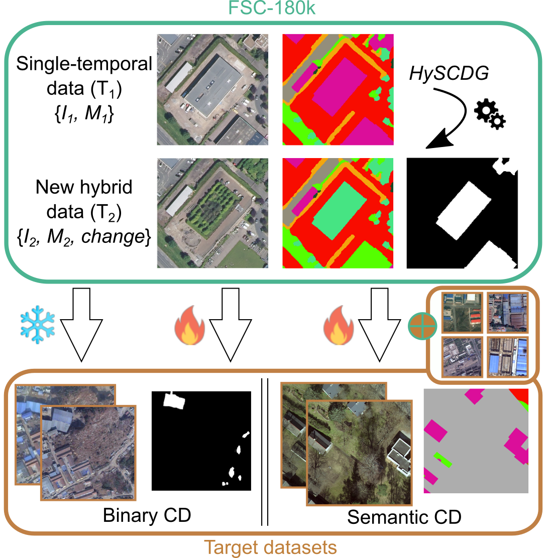
Figure 1: Efficient and scalable change detection requires a comprehensive training dataset that does not exist today. Using a single-temporal dataset (image+semantic map), we propose HySCDG  that generates a novel bi-temporal hybrid dataset FSC-180k. This enables multiple transfer learning possibilities on either binary and semantic change detection tasks. / : Transfer with/without fine-tuning our model, respectively.

Efficient methods for change detection (CD) are crucial for monitoring territories and the various phenomena and activities that impact them [3]. As human and climatic pressures increase, this topic is of utmost importance and calls every year for higher spatial resolution and semantic accuracy [55]. Change detection at scale has benefited greatly from the contributions of deep learning in recent years [12, 73, 69, 7], but most methods are grounded on large volumes of annotated data [60, 41]. Creating a large-scale dataset for bi-temporal (pair-wise) remote sensing change detection poses significant challenges and costs, especially when dealing with Very High Resolution (VHR) images (ground sampling distance: GSD $<$1 m, [30]). This is due to the need for expertise and considerable effort in collecting, preprocessing, and annotating images [59, 62], particularly in the case of VHR data and multiple labels (termed semantic change detection, SCD) [70, 74, 57, 61].

As an alternative, synthetic data generation is a promising direction for bi-temporal labeled data provision from a single temporal domain that is successful in diverse areas such as urban sprawl [17], disaster or climate change monitoring [42] or crop mapping [36]. Two main paradigms exist for CD: fully synthetic datasets (mainly graphics-based [27, 53]), and hybrid solutions that mix real and modified images, often at the instance level [5, 71, 69], known as data augmentation. The first method synthesizes image pairs by rendering two versions of a 3D virtual world thanks to a computer graphics engine. On the other hand, hybrid approaches synthesize new image pairs by pasting or erasing object instances into existing images (inpainting). They propose a suitable trade-off and faster generation of large quantities of data, with likely higher realism. However, none of these solutions meet the requirements for scalable SCD with VHR imagery (Tab. 1): focus on single tasks, restricted geographical areas, limited diversity, no guarantee on semantic consistency between pairs [48] and subsequently poor transfer to real datasets. To address this challenge, we introduce a generative pipeline built upon Stable Diffusion [44] and ControlNet [65], designed to harness an existing VHR semantic land cover dataset [18] and instance masks, to generate an extensive hybrid semantic bi-temporal change detection dataset encompassing both real and inpainted images, semantic land cover maps at each date, and a change map (Fig. 1). Then, we evaluate the transferability of our synthetic dataset on five datasets for both binary and semantic change detection cases ranging from zero-shot to sequential and mixed training set-ups, as well as under low-data regime.

Our contributions are as follows:

• We present a generation pipeline HySCDG  for creating VHR bi-temporal SCD datasets based on a land cover real-world dataset by using Stable Diffusion and ControlNet with tunable and semantically-guided inpainting of individual objects. It can be easily configured or finetuned on any land-cover dataset, generating images with the dataset’s distinctive traits.

• We provide FSC-180k: a Hybrid Semantic Change Detection pretraining dataset, created from FLAIR [18] along with the instance masks for 300k objects for the corresponding images.

• We provide a comprehensive evaluation of the proposed synthetic dataset on multiple transfer learning scenarios on five change datasets, in particular for SCD.

2 Related work

Detecting changes in the deep learning era.

We target bi-temporal land cover change detection in VHR images [32]. This historical task [22, 52, 37] consists in detecting the meaningful elements of a given area that have changed between two acquisitions and providing the land cover categories at each period (also known as change trajectory). It presents challenges: radiometric variations, geometric variations and non permanent changes. They have been extensively addressed with supervised deep learning techniques [70]: from CNN [12, 64, 11] to Transformers [72, 73, 7, 2, 13, 55], mainly with Siamese architecture. Multiple datasets, accompanied with ad-hoc methods, have been created to feed such models. They are often limited by their size [56, 6, 63, 39, 25], geographical extent [6, 63, 56, 57], low geometrical or annotation quality [11]. Also, most of the effort focuses on binary change detection, i.e., restricted to a unique category, mainly buildings [6, 50, 39, 25, 40] or disasters [67]. Such scarcity in high quality, diverse, large-scale labels is alleviated with transfer learning [51, 4], by fine-tuning models pretrained on large-scale datasets for different image domains, even for semantic change detection [63, 56, 57].

Synthesizing and inpainting remote sensing images.

Synthetic remote sensing data is useful e.g., for cloud removal [10], image restoration [16], or training deep supervised models [58], before transfer to real examples. Solutions based on patches, [35, 68], autoencoders [23], GAN [34, 28], pixel-aligned generation [24] have been proposed, but with limited image quality and no semantic control. Diffusion models (DM) have improved such quality [44], but most models have applied DM directly on mid-resolution RGB images [26, 14, 58], neglecting both the multi-spectral dimension [9] and VHR spaces. However, a key finding remains: semantically control the synthesis, e.g., by directly synthesizing text [26], semantic maps [58] or with a control module guided by edges [9], semantic maps [14] or metadata [26]. In our work, we fine-tune a Stable Diffusion and a ControlNet models to achieve semantically-controlled inpainting of VHR images as a basis to take advantage of existing images, and generate an hybrid semantic change detection dataset at scale and with high diversity.

Generating synthetic change datasets.

Two main approaches exist: fully synthetic or hybrid solutions. The first paradigm leverages advanced 3D rendering engines to create fully synthetic datasets [27, 17]. This procedural approach allows complete control over rendering parameters (instance placement, semantic classes, lighting conditions, etc.) generated from scratch. E.g., SyntheWorld [53] effectively leverages DM prompted by GPT-4 to create a diverse and large-scale fully synthetic dataset. On the other hand, hybrid approaches generate (semi-)synthetic data by inserting fake changes into real images.

Such modifications can be random crops [49], instance copy-pasting, or inpainting made by GAN [49, 71, 5] or DM [69, 54]. Blending or style transfer methods are often used to enhance diversity [5, 49].
A pivotal challenge is the semantic guidance: modifying few elements of images to mimic real scarce changes, e.g., with instance footprints extracted from external datasets [5] or segmentation model outputs [69]. [54] adopt a Denoising diffusion probabilistic model to generate a new image directly from a modified semantic map and a degraded version of the corresponding snapshot. Changen2 [69] is the closest work to ours, with a full pipeline to synthesize a hybrid semantic dataset, again with a DM conditioned by a semantic map. However, Changen2 creates synthetic data specific to a given target dataset in terms of image resolution, size, or change characteristics. In this paper, we explore semantically controlled inpainting based on DM and ControlNet to the intertwined challenge of diverse and multi-class modification of VHR images. It is termed HySCDG  and leads to the hybrid dataset named FSC-180k. Tab. 1 provides a comparison with main synthetic change detection datasets.

Table 1: Synthetic Change Datasets. Land cover change detection in remote sensing imagery. For the total number of pixels, we only consider strictly different images. The geographical zone’s extension can be local [regular], national flag: France or global . We denote open-access (OA) and directly downloadable datasets with ✔. In the case of IAug, we sum the number of pixels of the two datasets provided in this work. OEM means OpenEarthMap.

Dataset	OA	Pixels $\times 10^{6}$	GSD (m)	Classes	Source	Zone	Type
SynCW [27]	✗	37	0.6	1	X	[regular]	Synthetic
SMARS [17]	✔	110	0.3-0.5	2	X	[regular]	Synthetic
IAug [5]	✗	1,167	0.075-0.5	1	LEVIR-CD [6], WHU-CD [25]	[regular]	Hybrid
Ce-100K [54]	✗	6,553	0.25-0.5	8	OEM [62]		Synthetic
Changen2 [69]	✗	7,077	0.25–0.5	8	OEM [62]		Hybrid
Changen [71]	✗	11,796	0.8	1	xView2 [43]	[regular]	Hybrid
SyntheWorld [53]	✔	18,350	0.3-1	1	X	X	Synthetic
FSC-180k (Ours)	✔	80,740	0.2	16	FLAIR [18]	flag: France	Hybrid

Transfer learning from synthetic/hybrid datasets.

Transfer learning is used to assess the validity of the generated image pairs, and vary with the operational set-up [33]. SCD at scale is performed through sequential learning: pretraining on such datasets and fine-tuning on real-world cases [71, 69, 27, 5]. Fewer works [53] evaluate on mixed training sets (single training mixing both real and synthetic samples), which can help to prevent overfitting. An orthogonal solution considers low data regimes, i.e., fine-tuning on a very small train set [53, 54, 5], or even under zero-shot scenarios [54]. We evaluate our proposed dataset in the four conceivable transfer scenarios.

3 Hybrid generation of semantic changes

Much of the success of deep learning methods for Earth observation relies on large-scale training datasets with reliable annotations [18, 45]. However, no large-scale publicly available dataset exists for bi-temporal SCD: we propose HySCDG for Hybrid Semantic Change Detection Generation, a procedure to leverage existing large-scale land cover datasets and state-of-the-art image inpainting methods to simulate visually realistic bi-temporal semantic changes. This leads to the generation of the FSC-180k dataset.

Our paper is grounded on two main ideas: (i) Adapting and fine-tuning a Stable Diffusion Model enables efficient inpainting of VHR images with a semantic control and geographical instance selection; (ii) Changes can be simulated with sufficient diversity by randomly selecting instances (and modifying their labels) within an existing land cover map that is paired with the image used as input. The pipeline is shown in Fig. 2. Details are provided in the following.

Figure 2: HySCDG pipeline. From a single-temporal dataset composed of one VHR image $I_{1}$, a semantic map $M_{1}$, and some openly available labeled instances, we generate a new VHR image $I_{2}$, a new map $M_{2}$ and subsequently a change map $C$. This results in the FSC-180k  hybrid dataset. The two pivotal novelties consists in: (i) Adapting and fine-tuning a Stable-Diffusion Model from image inpainting and (ii) exploiting open geospatial data for inpainting prompt control and semantically guiding the objects to be modified. The combination of both solutions ensures a diverse at-scale VHR multi-class change detection dataset.

3.1 Adaptation of Stable Diffusion for Inpainting.

We use Stable Diffusion (SD) [44], an open and state-of-the-art text-to-image synthesis method. Our objective is to modify SD to manage controllable inpainting specifically in remote sensing aerial images, for various landscapes or semantic classes. Though SD models are effective in generating natural images with clear focal points and layered depth, with artistic or cinematic styles, they require adaptation to be used for remote sensing images [26]: acquisition distance, intricate textures, no domination of a single element. Starting from a Stable Diffusion 2 Inpainting checkpoint, we sequentially fine-tune the Autoencoder and the Diffusion U-Net, before adding and training a ControlNet [65] that leverages information extracted from an existing large-scale land cover dataset (namely, FLAIR [18], see Sec. 3.3). Our pipeline allows to generate 5-band images that incorporate infrared and elevation along with RGB channels, for the first time in satellite image synthesis.

Adaptation of the Variational Autoencoder.

Unlike most SD extensions, which focus on fine-tuning the central U-Net, we also adapted the Variational Autoencoder (VAE) that encodes images into the diffusion latent space. This adaptation targets efficient encoding of multi-band VHR images from the FLAIR dataset. The original VAE, trained with a KL-regularization factor [15], uses a combination of L1 and perceptual loss [66] alongside KL-divergence. To improve compression of remote sensing images, we added both L2 and Focal losses [31]: minimizing high-frequency errors reduces blurriness. Additionally, we included a “color loss” (L2 loss on each 55 patch) to limit oversaturation, which affects ground object color realism. Fine-tuning of the VAE took 160 hours A100 GPU.

Stable Diffusion training.

We then fine-tuned the Diffusion U-Net for inpainting, adapting it to the new VAE and teaching it to synthesize and inpaint VHR images. Special attention was given to prompt selection. Although inpainting is the model’s primary function, we included direct image generation from prompts in 10% to 20% of cases, as in standard SD. This training required 300 hours on a A100 GPU (30,000 iterations, batch size of 32).

Prompt Engineering.

Prompts are designed using both each image’s geographic coordinates and open land cover data (OpenStreetMap [38]). To avoid learning irrelevant details, prompts are composed of three elements: (i) Spatial (place name, city, region), (ii) Temporal (time of day, season), (iii) Semantic (frequent classes in the inpainted area, compared to the overall dataset).
Prompt example: “Grass and agricultural vegetation next to a highway, locality of Savigny-en-Revermont, Bourgogne-Franche-Comté, in the morning, during Summer.”

3.2 Conditional change inpainting with ControlNet

Driven by our goal to control the new classes in the inpainted zones, we add a ControlNet (CN) architecture [65] to build a model that generates realistic VHR images from a semantic segmentation map (here land cover). CN is designed to add task-specific conditioning to a pretrained image DM. It allows injecting explicit semantic guidance during the diffusion process, conditioning the outputs on some reference image (a color map of the semantic class), in addition to a text prompt. Our training method enables CN to perform both inpainting and text-to-image synthesis, using the semantic condition. Training took 240 hours on a A100 GPU.

3.3 Select, Mask, Change, Inpaint : the HySCDG  pipeline

Inspired by [46], the core of our method lies in our “Select and Inpaint” mechanism. Given a VHR image along with its semantic segmentation and instances, we inpaint these instances using the SD+CN inpainting method: the label of the instance is changed, the texture of the image is substituted accordingly. This results in a pair of VHR images, both with semantic maps and the corresponding semantic change maps. The complete HySCDG  is provided in Fig. 2 and detailed below. It is illustrated for one image but is applied several times to each image of the single temporal dataset.

HySCDG uncovered.

For an image $I_{1}$ with its semantic map $M_{1}$, and $\{O_{i}\}$ the set of $N_{I}$ instances lying on the extent of $I_{1}$.

• Randomly select $N_{change}$ instances among $\{O_{i}\}$.

• For each instance, generate an inpainting mask : footprint+spatial buffer.

• Using $M_{1}$, take as “$T_{1}$ class” the most frequent class inside the footprint: $c_{1}$. Then, select the larger convex hull of pixels of this class inside the buffered zone. These pixels correspond to the change mask: $C$.

• Randomly select another class $c_{2}$ at $T_{2}$ and replace the previous label by this new label.

• Randomly select $N_{nochange}$ random shapes in the image: such masks appear only on the inpainting mask, not on the change mask, letting their labels unchanged.

• Apply SD+CN to masked image and new semantic map.

• Cumulate the previous steps: we obtain our inpainting mask, change mask, and for $T_{2}$ a new semantic map $M_{2}$ and the corresponding new image $I_{2}$.

The pair of images ($I_{1}$, $I_{2}$) with their corresponding semantic maps ($M_{1}$, $M_{2}$), and the change map $C$ (difference between $M_{2}$ and $M_{1}$), are the samples of the hybrid dataset.

Label and instance extraction.

For comprehensive multi-class learning, we select FLAIR dataset [18], a large-scale semantic segmentation map for 16 land cover classes over more than 800 km². FLAIR offers the advantage of covering areas where geographical instances of many FLAIR labels are publicly available, alleviating requiring a panoptic segmentation. Around 300,000 instance masks have been extracted for this work.

Inpainting signature mitigation.

Inpainting produces realistic changes but new areas tend to have sometimes a high-frequency signature, as reported by other works [29, 20]. In order to discourage the model from simply learning this inpainting noise instead of learning the actual changes between images, we also inpaint random areas of the image without changing the semantic class in a similar way to the “not changed regions” from [46]. Besides, to obtain the best transition between the original image and the inpainted area, we use a continuous mask in the inference [1].

Selection of the new label.

For each change area, we randomly select the new class $c_{2}$ among all classes weighted by their frequency in the whole dataset divided by their frequencies in the change area.

Adoption of a buffer zone.

For inpainting, we add a buffer around the footprint of each modified instance. This gives SD more freedom to generate smoother borders around the changed areas. It also helps handling small spatial discrepancies between footprints and the VHR image content [19].

3.4 Structure of the FSC-180k dataset

For each image in the FLAIR training set, we generate three unique modified images, resulting in 180,000 synthetic images, each with a corresponding 512512 semantic map covering 16 distinct semantic classes. We call this dataset FSC-180k, short for FLAIR Synthetic Change. FSC-180k includes approximately 80 billion pixels with a ground resolution of 0.2 m per pixel. Note that we can expand the dataset by pairing synthetic images that were generated (differently) from a single real image, process that we use at training time, effectively doubling the number of image pairs. Tab. 1 compares FSC-180k with other synthetic change detection datasets and shows that FSC-180k offers a much broader range of semantic changes beyond simple building modifications, is of higher spatial resolution, and is nearly ten times larger than comparable datasets. It should also be noted that the proportion of changes in FSC-180k is closer to the real scenarios observed in Europe (prevalence of 5% change) than other academic datasets (see Tab. 2), excepting HiUCD.

Quality assessment of FSC-180k.

ControlNet is the most error-prone module: it may sometimes fail to respect the semantic map. We evaluated how unchanged the semantic map remains by performing 15-class semantic segmentation on real and generated images, thanks to a UNet trained for this task, leading to a satisfactory error rate below 20% between both outputs. We also leveraged standard metrics for image generation evaluation to assess the realism of the synthesis. We got an Inception Score [47] of 6.2 on the inpainted images, which is comparable to real images, and a low FID score [21] of 0.43 between inpainted and real images.

4 Experiments

We conduct various transfer learning experiments to validate hybrid data pretraining, comparing FSC-180k with the fully artificial SyntheWorld [53], the only available synthetic dataset with a size comparable to ours (see Tab. 1).

4.1 Pretraining approaches with FSC-180k

We assess FSC-180k’s effectiveness by exploiting existing open datasets as targets under various settings (see Tab. 2 and Supplementary Material). Here, we first present the different transfer learning approaches adopted, and then, dive into the deep models and datasets considered (Sec. 4.2). Our objective is to demonstrate how pretraining on a hybrid dataset improves performance, for both binary and semantic change detection.
The four scenarios are:

• Sequential Transfer Learning. Models are pretrained on FSC-180k, and then fine-tuned on the target data.

• Low Data Regime. The same as above but with a fraction of the available training set.

• Mixed Training. Models are trained on a blend of FSC-180k and the target data.

• Zero-Shot Learning. A model pretrained on FSC-180k is directly applied on the target dataset, with only a remapping of FSC-180k classes to align labels.

4.2 Experimental protocol

4.2.1 Target datasets and metrics

Our transfer experiments span five diverse datasets, among which three contain semantic labels (Tab. 2). This ensures variety in landscapes, sizes, and change types, i.e., a comprehensive evaluation. Among the plethora of (S)CD datasets, we selected the most popular ones: Levir-CD [6], S2Looking [50], SECOND [63] and HiUCD-mini [56].
We used classical metrics from the change detection literature: Intersection over Union (IoU) and F1 score for binary cases and mainly the Semantic Change Segmentation score (SCS) from [59] for semantic evaluation. In this latter case, the Separated Kappa (SeK) from [63] is also informative though it tends to be more biased towards detection task than semantic prediction.
We added some experiments related to HiUCD-XL [57], a follow-up dataset of HiUCD-mini [56] using semantic mIoU and change mIoU, metrics provided on the evaluation platform as test labels are kept private.

Table 2: Target datasets. Overview of the real-world datasets used for our transfer learning experiments.

Dataset	Change ($\%$)	Pixels $\times 10^{6}$	GSD (m)	Classes	Period	Zone
Levir-CD [6]	$28.4$	1,067	0.5	1	2002/18	Texas
S2Looking [50]	$25.6$	8,389	0.3-0.8	1	2017/20	World
SECOND [63]	$20.0$	1,222	0.3-0.6	6	?	China
HiUCD-mini [56]	$6.6$	567	0.1	9	2017/19	Estonia
HiUCD-XL [57]	$1.2$	10,695	0.1	9	2017/19	Estonia
FSC-180k  (Ours)	7.0	80,740	0.2	16	2018/21	France

4.2.2 Model architecture

We consider that designing a new architecture is out of the scope of this paper and that numerous solutions have already been proposed (see Sec. 2). Therefore, we initially used a simple U-Net model [8] with a segmentation head for semantic change detection. Although effective for binary change, it lacked expressiveness for semantic tasks. Similarly to [11], we developed a simple Dual UNet model composed of 2 nearly identical parallel UNets for (i) change detection, and (ii) semantic segmentation, with ResNet-50 backbones pretrained on ImageNet and trained in a multi-task setting. The change branch incorporates features from the semantic encoder. We keep the training strategy simple and constant to focus on data and transfer, this enhances interpretability.

Can a binary model be sufficient ?

We tested both a pure binary CD model and the Dual UNet, for which, when, switching to binary-only tasks, the semantic decoder is inactive but the encoding part remains active (as it provides features to the change detection branch). Such selective change detection ability allows training on a multi-class dataset and focusing on specific binary tasks. Experiments show that even for binary tasks, the Dual UNet outperforms the binary-only model, e.g., achieving an IoU of 0.83 on Levir-CD (compared to 0.80). Learning more information than just change pixels, the Dual UNet gains a deeper scene understanding, leading to more reliable predictions.

Existing architectures.

We tested more complex transformer-based architectures, namely ChangeFormer [2], MambaCD [7], and SCanNet [13], both on HiUCD-mini and SECOND datasets. SCanNet performed best, balancing high performance and straightforward implementation due to its lightweight design (see Supplementary Material). SCanNet is kept hereafter for comparisons (see Tab. G).

Transfer for varying semantic classes.

In the semantic case, we faced the issue of distinct classes between source and target datasets. This required to choose which classes should be kept for model training.

• Sequential case: for both pretraining and fine-tuning strategies, we use the classes of the processed dataset. The semantic head of the model is reinitialized and adapted to the new number of classes before fine-tuning.

• Mixed case: Classes from the target dataset are used, manually mapping pretraining classes to their closest counterparts.

4.2.3 Experimental setting

We apply basic augmentations on the images: horizontal and vertical flips, 90° rotations, and small rescaled crops (scales above 0.8). Normalization by mean and variance from the target dataset is used in all experiments. For optimization, we use the AdamW algorithm with default parameters (0.01 weight decay), and an initial learning rate of 3e-4 with exponential decay (0.99 per epoch). For sequential training, models are pretrained for 40h on a A100 GPU, with fine-tuning requiring up to 20h on a V100. For mixed training, we limit the total training time to 20h on a A100.

4.3 Results and Analysis

4.3.1 Sequential training

Binary Case.

Models pretrained on synthetic datasets outperform those without pretraining on all target datasets (Fig. 3). SyntheWorld maintains commendable performance on the the single-class “building” change case, similarly to Levir-CD. Pretraining on FSC-180k yields the strongest results, compared to SyntheWorld on all five target datasets, with gains of 2-3% of IoU. Details are provided in the Supplementary Material.

Figure 3: Sequential training in binary change detection. After pretraining our Dual U-Net on either nothing, SyntheWorld or FSC-180k, we finetune and test it on each of the 4 target datasets and represent the binary IoU.

Semantic Case.

Pretraining on FSC-180k outperforms the baseline and SyntheWorld on the three SCD datasets in the sequential mode (Tab. G). Indeed, pretraining on SyntheWorld, that focuses solely on the “building” class, shows limitations in multiclass tasks on HiUCD-mini and HiUCD-XL compared to the baseline. Our FSC-180k dataset is particularly beneficial for HiUCD-mini and HiUCD-XL. The types of landscapes and spatial resolution are relatively similar, which facilitates effective transfer learning. For HiUCD-mini, our pretraining results in a SeK of 0.19 and a SCS of 0.78, representing respective increases of 11% and 7% compared to the baseline. The gains rise to 28% and 8% against SyntheWorld. For SECOND, SyntheWorld partially narrows the gap: SeK of 0.17 and a SCS of 0.84, while the FSC-180k’s pretrained Dual UNet achieves 0.18 and 0.87.

Table 3: Sequential training in the semantic change detection framework. We report the binary change detection scores (IoU or Chg. mIoU) as well as semantic scores (SCS or mIoU) on three datasets in the sequential scheme. Models were initially pretrained (SyntheWorld or FSC-180k) or not (Baseline).

		SECOND		HiUCD-mini
Pretraining	Model	IoU	SCS	IoU	SCS
None	Dual UNet	0.53	0.83	0.61	0.73
SyntheWorld	Dual UNet	0.54	0.84	0.58	0.73
FSC-180k	Dual UNet	0.55	0.89	0.63	0.78
None	SCanNet	0.54	0.84	0.60	0.66
FSC-180k	SCanNet	0.56	0.89	0.63	0.71

	HiUCD-XL
Pretraining	Chg. mIoU	mIoU
None	0.17	0.58
SyntheWorld	0.17	0.58
FSC-180k	0.19	0.60

Dependence on a CD model.

We compared two CD model by running the same experiments on SECOND and HiUCD-mini with a SCanNet model (Tab. G). We were unable to reproduce the results reported in the original paper [13], despite following the described learning scheme. SCanNet still performs well on the SECOND dataset, achieving a SCS of 0.84, compared to 0.83 for the Dual UNet. The opposite trend is observed on HiUCD, where the Dual UNet reaches a SCS of 0.73, while SCanNet reaches 0.66. As neither of the two models stands out, we mainly present the results obtained with our Dual UNet.

4.3.2 Mixed training

Our experiments show, that the optimal ratio between synthetic and target data lies around 50% for HiUCD-XL, S2Looking or SECOND (Fig. 4) conversely to the conclusions in [53], where performance always increases with the amount of target data included in the training mix. Nevertheless, the optimal ratio is 90% for smaller dataset such as Levir-CD or HiUCD-mini, that may be too specific. However, the mixed training strategy proves to be really effective, outperforming the sequential one on HiUCD-XL with a balanced blend as training base, as noticed in Fig. 4, compared to Tab. G. We can deduce that:

• Sequential training maybe suboptimal: The lengthy fine-tuning process can lead the model to “forget” pretraining, and instead overfits on the target data, which finally reduces the benefits of pretraining.

• In contrast, mixed training augments the initial set and adds diversity throughout the training process. The model sees as many images from the target dataset as in the sequential mode, but continues to benefit from the pretraining dataset.

• A “balanced blend” of synthetic and target data appears optimal, providing a sufficient frequency of target images for exploitation while strategically incorporating new synthetic images to enable exploratory learning and notably avoid overfitting.

Figure 4: Mixed training (Binary and Semantic). Training on a blend of target and synthetic/hybrid (SyntheWorld or FSC-180k) train sets, containing a ratio of x% samples from the target (including repetitions). Testing is performed on the target test set. 100% corresponds to fine-tuning exclusively on target dataset (without pretraining).

4.3.3 Low Data regime

We apply a sequential scheme but limit fine-tuning to small subsets of the target data: specifically, 1%, 10%, and 30% of the training set. Each experiment was repeated 10 times, with a random sampling of the training set. We consider these to be the most meaningful experiments, as this scenario closely matches real-world use cases. The primary objective of pretraining is to develop a model that can either swiftly adapt to new target datasets or perform well when only limited training data is available. One can observe on Fig. 5 a clear advantage for pretrained models at very low level (1%). With such little data, the model cannot fully learn the specificities of the target dataset and relies primarily on its general knowledge and on the task itself (detecting changes), rather than on dataset-specific features. Unsurprisingly, models pretrained for this task perform significantly better. However, as the amount of available data increases, the gap tends to narrow. Models increasingly rely on data itself, to which they have equal access, yet pretraining on FSC-180k still yields better performance than using SyntheWorld or training from scratch.

Figure 5: Low data regime (Semantic). Fine-tuning on a limited part of the target train set (either 1%, 10% or 30% of randomly sampled examples) and evaluating on the whole test set. Models are initially pretrained (SyntheWorld or FSC-180k) or not (Baseline). Metrics are averaged on 10 runs for SECOND and HiUCD-mini.

4.3.4 Zero-Shot evaluation

While models pretrained on SyntheWorld struggle to transfer effectively without target sample exposure, pretraining on FSC-180k delivers respectable results, achieving IoU scores of 0.37 on SECOND and 0.36 on HiUCD-mini, showing performance drops of 31% and 40%, compared to the fully supervised models (details are provided in the Supplementary Material). However, FSC-180k is less effective on Levir-CD, where the performance drop reaches 60% (0.33 vs. 0.83 IoU). We argue that performance in this scenario is directly linked to dataset similarities: the limited realism in SyntheWorld hinders transferability, while FSC-180k’s diverse landscapes and sparse changes further limit its effectiveness. For the semantic task, pretraining on FSC-180k enhances the model’s understanding of change trajectories, achieving SCS of 0.24 on SECOND and 0.25 on HiUCD-mini.

4.3.5 Qualitative assessment

Qualitative analysis of the various segmentation results indicates that FSC-180k pretraining significantly enhances the network’s ability to localize features in input images. This improvement leads to both more accurate segmentation within VHR images and higher semantic prediction accuracy for main classes of interest in the semantic case (e.g., buildings, roads, bare land for HiUCD-mini, buildings or non-vegetated ground surface for SECOND). Qualitative examples for the different datasets are provided in the Supplementary Material.

5 Conclusion

We introduced HySCDG, a new, simple bi-temporal change detection generation pipeline. It lies on Stable Diffusion and ControlNet for creating hybrid content of VHR images. HySCDG leverages an existing large-scale semantic land cover map to overcome the lack of diversity and size of real-world datasets. We provide FSC-180k , a pretraining dataset based on FLAIR [18], which includes bi-temporal real/inpainted images, and their associated semantic maps. The proposed solution was evaluated for transferability, on five datasets over four distinct training setups. Our experiments on both binary and semantic cases demonstrated strong transferability, confirming FSC-180k robustness and adaptability as well as HySCDG relevance.

Supplementary Material

In this appendix, we provide implementation details in Sec. A, details about the deep architecture used in Sec. C and detailed quantitative results in Sec. D. Finally, we provide qualitative samples in Sec. E.

Figure A: Transfer Learning scenarios. We illustrate here the various configurations tested and described in Sec. 4.1.

A Implementation Details

A.1 Training of Stable Diffusion

For the VAE training, the color loss was applied only after a sufficient amount of 50,000 iterations. Fine-tuning the VAE took 160 hours A100 GPU for a total of 500,000 iterations with a batch size of 4. The diffusion UNet training required 300 hours A100 GPUs, for a total of 30,000 iterations with a batch size of 32. The training was run on 4 GPU in parallel. Finally, we trained the ControlNet for 240 hours on a A100 GPU, performing 45,000 iterations with a batch size of 16. We also observed the “sudden convergence phenomenon” mentioned in [65].

A.2 The HySCDG pipeline details

In the HySCDG pipeline, for a given image with $n$ instances, we randomly select $N_{change}$ instances (from 0 to $min(3,n)$) to inpaint with a semantic class change and $N_{nochange}$ (from 0 to $min(3,n)$) random shapes for inpainting without semantic class change. We draw the number of instances and shapes from the following heuristical laws (Eqs. A and B):

$$N_{change}\sim\left\lfloor\sqrt{\mathcal{U}(0,10)}\right\rfloor,$$ (A)

$$N_{nochange}\sim\left\lfloor\sqrt{\mathcal{U}(0,10)\times(1-\frac{N_{change}}{4})}\right\rfloor.$$ (B)

The frequency of the inpainted instances and random shapes can be seen in Fig. B function to $n$ the number of instances within the image.

Number of instances in the footprint of a given image

Figure B: Heuristic rule to define instance and random mask numbers. We illustrated the frequency of the number of instances inpainted (rows) and the number of random shapes inpainted (columns) with respect to the number $n$ of instances contained in the footprint of the VHR images.

A.3 FLAIR Dataset [18]

The FLAIR dataset [18] is composed of 77,762 VHR aerial patches 512 512 at 0.20m GSD. The VHR images include five channels: Red, Green, Blue, near-infrared, and a normalized Digital Surface Model derived by dense image matching (normalization means the altitude of the terrain is removed). For each patch, ground truth semantic segmentation is provided. The semantic map represents the land cover based on a 19 classes nomenclature (building, coniferous, deciduous, etc. details provided in Fig. 2). We only use the 16 main classes due to the scarcity of certain classes or potential ambiguity. This dataset covers approximately 817km² extracted from various areas in France.

A.4 Training computing times

Models were pretrained to convergence on the synthetic datasets, requiring 40 to 60 hours on a A100 GPU, depending on the configuration. For instance, Dual UNet converges faster than SCanNet, multi-task learning takes longer than binary-only, and the larger size of FSC-180k compared to SyntheWorld requires additional iterations.

For the sequential scenario, fine-tuning was done in 10 to 20 hours (V100 GPU) for HiUCD-mini, Levir-CD, S2Looking and SECOND (in increasing order) and 20 hours (A100 GPU) for HiUCD-XL. For mixed training, all trainings took from 16 to 20 hours (A100 GPU). Note that, in low data regime, each experiment was repeated 10 times, except for HiUCD-XL for which it was only 3 times for 10% and 30% experiments.

B Failure cases of the HySCDG synthesis

ControlNet is the most error-prone module as it may fail to respect the semantic map. Other elements are more reliable or less sensitive: instance footprints of high quality, low influence of text prompt, high-quality inpainting from SD alone (Figure C). In this same figure, we show results with only the ControlNet module fine-tuned for generating aerial images from semantic maps, revealing a cartoonish style.

Failure cases of HySCDG		Only ControlNet trained

Figure C: Illustrations of failure cases of synthesis with our pipeline HySCDG, and synthesis with only the ControlNet trained.

C Pretraining and transfer experiments

C.1 Transfer Learning Scenarios

The four transfer learning scenarios considered in this work are illustrated on Fig. A. They are quantitatively detailed in Section D.

Table A: Comparison of model architectures The different models were evaluated on SECOND and HiUCD-mini after being trained from scratch for the same duration. Bold values correspond to the best values for each metric and each dataset.

Target	Model	IoU	SeK
SECOND	MambaCD	0.52	0.14
	SCanNet	0.54	0.19
	Simple UNet	0.51	0.11
	Dual UNet	0.53	0.16
HiUCD mini	MambaCD	0.53	0.08
	SCanNet	0.62	0.11
	Simple UNet	0.50	0.07
	Dual UNet	0.61	0.17

C.2 Model architectures

Our Dual UNet architecture consists of two parallel UNet-style auto-encoders: one dedicated to semantic segmentation for each image separately, and the other one for detecting changes by processing concatenated image pairs. Both UNets share the same core configuration, differing only in their input and output layers: the change detection UNet takes two concatenated images as input and outputs two classes (no-change, change), while the semantic segmentation UNet processes single images and outputs the number of semantic classes (of the dataset). Both networks use a ResNet-50 encoder pretrained on the ImageNet dataset. To enhance performance, features extracted at each encoding step of the semantic UNet are injected into the decoding pathway of the change detection UNet, in addition to its own skip connection features. The entire model comprises a total of 83 million parameters.

We compared our architecture with state-of-the-art change detection models that rely on different mechanisms: MambaCD [7], SCanNet [13], and ChangeFormer [2]. The latter, ChangeFormer was only evaluated through pretraining on FSC-180k, which proved unsuccessful due to the model’s excessive size and the significant computational resources required for training. MambaCD and SCanNet were evaluated on SECOND and HiUCD-mini. The performances of the different models can be found in Tab. A. SCanNet was better in all cases and was therefore kept for comparison in sequential experiments, with FSC-180k pretraining.

C.3 Normalization

We compared the effects of applying or not normalization by mean and variance of the train set pixel’s values on the input data. It proved to be really effective. For example, this improves SCanNet’s performance on the SECOND dataset from 0.17 to 0.19 in Separated Kappa. We used it in all our experiments, using the parameters of the handled dataset. Namely, in sequential mode, normalization uses the synthetic dataset’s parameters during pretraining, and the target dataset parameters during fine-tuning.

Table B: Effect of the normalization. The impact of input normalization was evaluated on the SECOND dataset. For both SCanNet and Dual UNet, normalization was highly effective.

Model	Normalization	IoU	SeK
SCanNet		0.52	0.17
	X	0.54	0.19
Dual UNet		0.51	0.14
	X	0.53	0.16

D Quantitative results

In this section, we present in details the quantitative results for both binary and semantic cases, for the four transfer learning scenarios. We follow the same order as in the paper.

• Sequential Training: binary change detection (BCD) results are provided in Tab. C, while semantic change detection (SCD) outputs are given in Tab. G.

• Low-Data Regime: results for BCD can be found in Tab. D for Levir-CD et S2Looking, and in Tab. H for SECOND and HiUCD-mini for the SCD configuration.

• Mixed Training: Tab. E and Tab. I provide numbers, respectively, for BCD for the four datasets and SCD for SECOND and HiUCD-mini datasets. Tab. J focuses on HiUCD-XL dataset.

• Zero-Shot Learning: results for BCD and SCD are given in Tab. F and Tab. K respectively.

D.1 Binary change detection

Table C: Sequential Training Evaluation (Binary Change Detection). We report the F1 and IoU scores on four datasets. Models were initially pretrained (SyntheWorld or FSC-180k) or not (Baseline) and then fine-tuned on the target dataset. Pretraining effects remain limited on simpler datasets such as Levir-CD, but provide significant benefits for more complex datasets like HiUCD, which is also closer to our FSC-180k in terms of landscapes and characteristics. Bold values correspond to the best values for each metric and each dataset.

	Target Pretraining $\downarrow$	Levir-CD	S2Looking	SECOND	HiUCD mini
F1	Baseline	0.91	0.61	0.70	0.75
	SyntheWorld	0.91	0.63	0.71	0.73
	FSC-180k	0.91	0.63	0.71	0.77
IoU	Baseline	0.83	0.44	0.53	0.61
	SyntheWorld	0.84	0.46	0.54	0.58
	FSC-180k	0.84	0.46	0.55	0.63

Table D: Low Data Regime (Binary Change Detection). We report the IoU scores on two binary datasets. Models were initially pretrained (SyntheWorld or FSC-180k) or not (Baseline) and then fine-tuned on a portion of the target dataset (X%). Pretraining offers significant advantages in scenarios with limited data, making it particularly valuable in many real-world applications. Bold values correspond to the best values for each metric and each dataset.

Target Percent	1 %	10 %	30 %
Levir-CD
Baseline	0.36	0.69	0.75
SyntheWorld	0.41 (+14%)	0.71 (+3%)	0.77 (+3%)
FSC-180k	0.55 (+53%)	0.73 (+6%)	0.79 (+5%)
S2Looking
Baseline	0.10	0.27	0.38
SyntheWorld	0.08 (-20%)	0.34 (+26%)	0.41 (+8%)
FSC-180k	0.15 (+50%)	0.36 (+33%)	0.43 (+13%)

Table E: Mixed Training Evaluation (Binary Change Detection). Model are trained on a blend of target and synthetic/hybrid (SyntheWorld or FSC-180k) train sets, containing a ratio of x% samples from the target (including repetitions). Testing is performed on the target test set. The last column corresponds to train exclusively on target dataset (without pretraining). We report the F1 and IoU scores on four datasets. Mixed training turns out to be at least as effective as sequential one. Bold values correspond to the best values for each metric and each dataset.

Target		Pretraining	20%	50%	90%	100%
Levir-CD	F1	SyntheWorld	0.90	0.90	0.91	0.90
		FSC-180k	0.90	0.91	0.91
	IoU	SyntheWorld	0.81	0.83	0.84	0.83
		FSC-180k	0.82	0.83	0.84
S2Looking	F1	SyntheWorld	0.60	0.63	0.62	0.61
		FSC-180k	0.61	0.64	0.63
	IoU	SyntheWorld	0.43	0.48	0.48	0.44
		FSC-180k	0.44	0.49	0.49
SECOND	F1	SyntheWorld	0.71	0.72	0.71	0.70
		FSC-180k	0.72	0.73	0.72
	IoU	SyntheWorld	0.54	0.56	0.55	0.53
		FSC-180k	0.57	0.57	0.55
HiUCD mini	F1	SyntheWorld	0.71	0.72	0.72	0.75
		FSC-180k	0.76	0.76	0.77
	IoU	SyntheWorld	0.58	0.58	0.59	0.61
		FSC-180k	0.61	0.62	0.63

Table F: Zero-Shot Evaluation (Binary Change Detection). We report the F1 and IoU scores for the zero-shot case. Metrics for SECOND and HiUCD are available on Tab. K. Models were initially pretrained (SyntheWorld or FSC-180k). Decent performance was obtained on Levir-CD, despite the domain gap between FSC-180k and Levir-CD. However, pretraining remained completely ineffective for S2Looking. Bold values correspond to the best values for each metric and each dataset.

Target	Pretraining	F1	IoU
Levir-CD	SyntheWorld	0.25	0.13
	FSC-180k	0.49	0.33
S2Looking	SyntheWorld	0.0	0.0
	FSC-180k	0.04	0.02

D.2 Semantic change detection

Table G: Sequential Training Evaluation (Semantic Change Detection). We report the binary and semantic scores on three datasets. Models (based on the Dual UNet) were initially pretrained (SyntheWorld or FSC-180k) or not (Baseline), and, then, fine-tuned on the target dataset. Pretraining on FSC-180k proved highly effective and outperformed SyntheWorld on every semantic dataset, with greater benefits observed on HiUCD due to the higher similarity between the datasets. Bold values correspond to the best values for each metric and each dataset.

Target	Pretraining	IoU	Ovr. IoU	SeK	SCS
SECOND	Baseline	0.53	0.64	0.16	0.83
	SyntheWorld	0.54	0.63	0.17	0.84
	FSC-180k	0.55	0.65	0.18	0.89
HiUCD mini	Baseline	0.61	0.77	0.17	0.73
	SyntheWorld	0.58	0.78	0.15	0.73
	FSC-180k	0.63	0.79	0.19	0.78
		Sem. mIoU	Chg. mIoU	Bin. mIoU	Bin. C. mIoU
HiUCD XL	Baseline	0.58	0.17	0.34	0.48
	SyntheWorld	0.58	0.17	0.34	0.48
	FSC-180k	0.60	0.19	0.34	0.48

Table H: Low Data Regime (Semantic Change Detection). Models were initially pretrained (SyntheWorld or FSC-180k) or not (Baseline) and then fine-tuned on a portion of the target dataset (x%). The benefit of pretraining increases as the amount of available data decreases. These experiments highlight the relevance of pretraining on our FSC-180k in real-world cases where annotated data is often scarce and/or costly to obtain. Bold values correspond to the best values for each metric and each dataset.

Target Percent	1 %	10 %	30 %
SECOND (scores in SCS)
Baseline	0.31	0.49	0.69
SyntheWorld	0.37 (+18%)	0.49 (+0%)	0.64 (-6%)
FSC-180k	0.40 (+29%)	0.57 (+15%)	0.74 (+8%)
HiUCD-mini (scores in SCS)
Baseline	0.13	0.41	0.48
SyntheWorld	0.17 (+31%)	0.38 (-7%)	0.50 (+4%)
FSC-180k	0.20 (+38%)	0.49 (+19%)	0.54 (+13%)
HiUCD-XL (scores in Chg. mIoU)
Baseline	0.06	0.10	0.12
SyntheWorld	0.05 (-16%)	0.10 (+0%)	0.11 (-8%)
FSC-180k	0.08 (+33%)	0.13 (+30%)	0.15 (+25%)

Table I: Mixed Training Evaluation (Semantic Change Detection). Model are trained on a blend of target and synthetic/hybrid (SyntheWorld or FSC-180k) train sets, containing a ratio of x% samples from the target (including repetitions). Testing is performed on the target test set. The last column corresponds to train exclusively on target dataset (without pretraining). Mixed training turns out to be more effective than sequential training, thanks to the exposure of the model to diverse and varied examples throughout the training process. Bold values correspond to the best values for each metric and each dataset.

Target		Pretraining	20%	50%	90%	100%
SECOND	IoU	SyntheWorld	0.54	0.56	0.55	0.53
		FSC-180k	0.57	0.57	0.55
	Ovr. IoU	SyntheWorld	0.61	0.62	0.63	0.64
		FSC-180k	0.64	0.63	0.62
	SeK	SyntheWorld	0.16	0.17	0.16	0.16
		FSC-180k	0.19	0.18	0.18
	SCS	SyntheWorld	0.83	0.84	0.85	0.83
		FSC-180k	0.88	0.89	0.88
HiUCD mini	IoU	SyntheWorld	0.58	0.58	0.59	0.61
		FSC-180k	0.61	0.62	0.63
	Ovr. IoU	SyntheWorld	0.74	0.78	0.77	0.77
		FSC-180k	0.76	0.77	0.77
	SeK	SyntheWorld	0.11	0.13	0.14	0.17
		FSC-180k	0.16	0.17	0.18
	SCS	SyntheWorld	0.68	0.71	0.72	0.73
		FSC-180k	0.74	0.76	0.78

Table J: Mixed Training Evaluation on HiUCD-XL. Training on a blend of target and synthetic/hybrid (SyntheWorld or FSC-180k) train sets, containing a ratio of x% samples from the target (including repetitions). Testing is performed on the target test set. 100% corresponds to fine-tuning exclusively on target dataset (without pretraining). 0% corresponds to zero-shot (after pretraining). An optimal mix ratio appears to be around 50%, which can be understood as a good compromise between exploration (pretraining data) and exploitation (target data). Bold values correspond to the best values for each metric.

Pretraining	Mix ratio	Sem. mIoU	Chg. mIoU	Bin. mIoU	Bin. C. mIoU
SyntheWorld	0%	0.02	0.03	0.0	0.47
	20%	0.51	0.10	0.33	0.48
	50%	0.62	0.19	0.37	0.51
	90%	0.60	0.17	0.32	0.47
FSC-180k	0%	0.35	0.07	0.20	0.43
	20%	0.58	0.15	0.32	0.51
	50%	0.63	0.20	0.29	0.52
	90%	0.62	0.18	0.30	0.51
-	100%	0.58	0.17	0.34	0.48

Table K: Zero-Shot Evaluation (Semantic Change Detection). Models were initially pretrained (SyntheWorld or FSC-180k). In semantic mode, only FSC-180k pretraining enables the model to detect changes and predict semantic segmentation. Bold values correspond to the best values for each metric and each dataset.

Target	Pretraining	F1	IoU	SCS
SECOND	SyntheWorld	0.02	0.01	0.0
	FSC-180k	0.53	0.36	0.24
HiUCD mini	SyntheWorld	0.02	0.01	0.0
	FSC-180k	0.53	0.36	0.25
		Sem. mIoU	Chg mIoU	Bin. mIoU
HiUCD XL	SyntheWorld	0.02	0.03	0.0
	FSC-180k	0.35	0.07	0.20

E Qualitative results

In Fig. D, we provide some examples of images generates with HySCDG, that we extracted from our dataset FSC-180k. One can see the joint spatial and semantic accuracy of the images and maps, coupled with diverse and real-world change configurations. The random selection of instances allows to provide multiple change trajectories and not to focus on main classes (namely, Building, Impervious surfaces, and Bare soil). The controlled inpainting is fairly realistic, for example with the addition of an agricultural field to replace a sport ground at the top right of the first line image.

Figure D: FSC-180k samples. Hybrid change pair images from our pretraining dataset, generated by HySCDG. The first column $T_{1}$ corresponds to the unpainted images, the second to the corresponding semantic map $M_{1}$, the middle column provides the change map, whereas the two last columns are the FLAIR samples used for generating the three first elements from the row (VHR image and semantic map). Best viewed in color.

Fig. E and Fig. F provide several examples of semantic prediction results with our Dual UNet architecture for SECOND and HiUCD-mini datasets, respectively. Experiments were performed in sequential scenario: without synthetic nor hybrid training data (Baseline), pretraining on SyntheWorld, and pretraining on FSC-180k.
One can first see that the Dual UNet architecture alone is sufficient for reliable dense predictions on VHR images, validating our quantitative assessment related to model architectures (Tab. A). Secondly, it can be noticed that working with FSC-180k allows for more consistent results over various classes, landscapes, and datasets. It is also worth noting that the GSD varies between the pretraining dataset (0.2m) and the target datasets (0.1m for HiUCD and approximately 0.45m for SECOND).

Figure E: Qualitative change detection on the SECOND dataset. For each pair of images, we show the land cover prediction and the binary change detection maps for models pretrained on (SyntheWorld or FSC-180k [Ours]) or not (Baseline) and then fine-tuned on the target dataset, in a sequential manner. The second column is composed of the ground truth maps. Best viewed in color.

Figure F: Qualitative change detection on the HiUCD-mini dataset. For each pair of images, we show the land cover prediction and the binary change detection maps for models pretrained on (SyntheWorld or FSC-180k [Ours]) or not (Baseline) and then fine-tuned on the target dataset, in a sequential manner. The second column is composed of the ground truth maps. Best viewed in color.

References

- [1] Andrew. How to use Soft Inpainting - Stable Diffusion Art. https://stable-diffusion-art.com/soft-inpainting/, 2024.
- [2] Wele Gedara Chaminda Bandara and Vishal M. Patel. A transformer-based siamese network for change detection. In IGARSS, pages 207–210, 2022.
- [3] Marshall Burke, Anne Driscoll, David B. Lobell, and Stefano Ermon. Using satellite imagery to understand and promote sustainable development. Science, 371(6535), 2021.
- [4] Yinxia Cao and Xin Huang. A full-level fused cross-task transfer learning method for building change detection using noise-robust pretrained networks on crowdsourced labels. Remote Sensing of Environment, 284:113371, 2023.
- [5] Hao Chen, Wenyuan Li, and Zhenwei Shi. Adversarial instance augmentation for building change detection in remote sensing images. IEEE Transactions on Geoscience and Remote Sensing, 60:1–16, 2021.
- [6] Hao Chen and Zhenwei Shi. A spatial-temporal attention-based method and a new dataset for remote sensing image change detection. Remote Sensing, 12(10), 2020.
- [7] Hongruixuan Chen, Jian Song, Chengxi Han, Junshi Xia, and Naoto Yokoya. Changemamba: Remote sensing change detection with spatiotemporal state space model. IEEE Transactions on Geoscience and Remote Sensing, 62:1–20, 2024.
- [8] Isaac Corley, Caleb Robinson, and Anthony Ortiz. A change detection reality check. arXiv preprint arXiv:2402.06994, 2024.
- [9] Mikolaj Czerkawski and Christos Tachtatzis. Exploring the capability of text-to-image diffusion models with structural edge guidance for multi-spectral satellite image inpainting. IEEE Geoscience and Remote Sensing Letters, 2024.
- [10] Mikolaj Czerkawski, Priti Upadhyay, Christopher Davison, Astrid Werkmeister, Javier Cardona, Robert Atkinson, Craig Michie, Ivan Andonovic, Malcolm Macdonald, and Christos Tachtatzis. Deep internal learning for inpainting of cloud-affected regions in satellite imagery. Remote Sensing, 14(6):1342, 2022.
- [11] Rodrigo Caye Daudt, Bertrand Le Saux, Alexandre Boulch, and Yann Gousseau. Multitask learning for large-scale semantic change detection. Computer Vision and Image Understanding, 187:102783, 2019.
- [12] Rodrigo Caye Daudt, Bertrand Le Saux, and Alexandre Boulch. Fully convolutional siamese networks for change detection. In ICIP, pages 4063–4067, 2018.
- [13] Lei Ding, Jing Zhang, Haitao Guo, Kai Zhang, Bing Liu, and Lorenzo Bruzzone. Joint spatio-temporal modeling for semantic change detection in remote sensing images. IEEE Transactions on Geoscience and Remote Sensing, 62:1–14, 2024.
- [14] Miguel Espinosa and Elliot J. Crowley. Generate your own scotland: Satellite image generation conditioned on maps. NeurIPS 2023 Workshop on Diffusion Models, 2023.
- [15] Patrick Esser, Robin Rombach, and Bjorn Ommer. Taming transformers for high-resolution image synthesis. In CVPR, pages 12873–12883, 2021.
- [16] Weiliang Fan, Jing M Chen, and Weimin Ju. A pixel missing patch inpainting method for remote sensing image. In International Conference on Geoinformatics, 2011.
- [17] Mario Fuentes Reyes, Yuxing Xie, Xiangtian Yuan, Pablo d’Angelo, Franz Kurz, Daniele Cerra, and Jiaojiao Tian. A 2D/3D multimodal data simulation approach with applications on urban semantic segmentation, building extraction and change detection. ISPRS Journal of Photogrammetry and Remote Sensing, 205:74–97, 2023.
- [18] Anatol Garioud, Nicolas Gonthier, Loic Landrieu, Apolline De Wit, Marion Valette, Marc Poupée, Sebastien Giordano, and Boris Wattrelos. FLAIR : a country-scale land cover semantic segmentation dataset from multi-source optical imagery. In NeurIPS Datasets and Benchmarks Track, 2023.
- [19] Adrien Gressin, Nicole Vincent, Clément Mallet, and Nicolas Paparoditis. Semantic approach in image change detection. In ACIVS, 2013.
- [20] Xiao Guo, Xiaohong Liu, Zhiyuan Ren, Steven Grosz, Iacopo Masi, and Xiaoming Liu. Hierarchical fine-grained image forgery detection and localization. In CVPR, 2023.
- [21] Martin Heusel, Hubert Ramsauer, Thomas Unterthiner, Bernhard Nessler, and Sepp Hochreiter. Gans trained by a two time-scale update rule converge to a local nash equilibrium. Advances in neural information processing systems, 30, 2017.
- [22] Philip J Howarth and Gregory M Wickware. Procedures for change detection using landsat digital data. International Journal of Remote Sensing, 2(3):277–291, 1981.
- [23] Wenli Huang, Ye Deng, Siqi Hui, and Jinjun Wang. Image inpainting with bilateral convolution. Remote Sensing, 14(23):6140, 2022.
- [24] Phillip Isola, Jun-Yan Zhu, Tinghui Zhou, and Alexei A Efros. Image-to-image translation with conditional adversarial networks. In IEEE Conference on Computer Vision and Pattern Recognition (CVPR), pages 1125–1134, 2017.
- [25] Shunping Ji, Shiqing Wei, and Meng Lu. Fully convolutional networks for multisource building extraction from an open aerial and satellite imagery data set. IEEE Transactions on Geoscience and Remote Sensing, 57(1):574–586, 2018.
- [26] Samar Khanna, Patrick Liu, Linqi Zhou, Chenlin Meng, Robin Rombach, Marshall Burke, David B Lobell, and Stefano Ermon. Diffusionsat: A generative foundation model for satellite imagery. In ICLR, 2023.
- [27] Maria Kolos, Anton Marin, Alexey Artemov, and Evgeny Burnaev. Procedural synthesis of remote sensing images for robust change detection with neural networks. In Advances in Neural Networks, 2019.
- [28] Andrey Kuznetsov and Mikhail Gashnikov. Remote sensing image inpainting with generative adversarial networks. In ISDFS, 2020.
- [29] Ang Li, Qiuhong Ke, Xingjun Ma, Haiqin Weng, Zhiyuan Zong, Feng Xue, and Rui Zhang. Noise doesn’t lie: towards universal detection of deep inpainting. In IJCAI, 2021.
- [30] Zhuohong Li, Wei He, Jiepan Li, Fangxiao Lu, and Hongyan Zhang. Learning without exact guidance: Updating large-scale high-resolution land cover maps from low-resolution historical labels. In CVPR, 2024.
- [31] Tsung-Yi Lin, Priya Goyal, Ross Girshick, Kaiming He, and Piotr Dollár. Focal loss for dense object detection. IEEE Transactions on Pattern Analysis and Machine Intelligence, 42(2):318–327, 2020.
- [32] Zhiyong Lv, Tongfei Liu, Jón Atli Benediktsson, and Nicola Falco. Land cover change detection techniques: Very-high-resolution optical images: A review. IEEE Geoscience and Remote Sensing Magazine, 10(1):44–63, 2021.
- [33] Yuchi Ma, Shuo Chen, Stefano Ermon, and David B Lobell. Transfer learning in environmental remote sensing. Remote Sensing of Environment, 301:113924, 2024.
- [34] Javier Marín and Sergio Escalera. Sssgan: Satellite style and structure generative adversarial networks. Remote Sensing, 13(19):3984, 2021.
- [35] Fan Meng, Xiaomei Yang, Chenghu Zhou, and Zhi Li. A sparse dictionary learning-based adaptive patch inpainting method for thick clouds removal from high-spatial resolution remote sensing imagery. Sensors, 17(9):2130, 2017.
- [36] Ali Mirzaei, Hossein Bagheri, and Iman Khosravi. Enhancing crop classification accuracy through synthetic SAR-Optical data generation using deep learning. ISPRS International Journal of Geo-Information, 12(11), 2023.
- [37] Hassiba Nemmour and Youcef Chibani. Multiple support vector machines for land cover change detection: An application for mapping urban extensions. ISPRS Journal of Photogrammetry and Remote Sensing, 61(2):125–133, 2006.
- [38] OpenStreetMap contributors. Planet dump retrieved from https://planet.osm.org . https://www.openstreetmap.org, 2017.
- [39] Chao Pang, Jiang Wu, Jian Ding, Can Song, and Gui-Song Xia. Detecting building changes with off-nadir aerial images. Science China Information Sciences, 66(4):140306, 2023.
- [40] Daifeng Peng, Lorenzo Bruzzone, Yongjun Zhang, Haiyan Guan, Haiyong Ding, and Xu Huang. Semicdnet: A semisupervised convolutional neural network for change detection in high resolution remote-sensing images. IEEE Transactions on Geoscience and Remote Sensing, 59(7):5891–5906, 2020.
- [41] R.S. Priya and K. Vani. Vegetation change detection and recovery assessment based on post-fire satellite imagery using deep learning. Nature Sci Rep, 14:12611, 2024.
- [42] Xiaofan Qu, Feng Gao, Junyu Dong, Qian Du, and Heng-Chao Li. Change detection in synthetic aperture radar images using a dual-domain network. IEEE Geoscience and Remote Sensing Letters, 19:1–5, 2022.
- [43] Gupta Ritwik, Hosfelt Richard, Sajeev Sandra, Patel Nirav, Goodman Bryce, Doshi Jigar, Heim Eric, Choset Howie, and Gaston Matthew. xbd: A dataset for assessing building damage from satellite imagery. arXiv preprint arXiv:1911.09296, 2019.
- [44] Robin Rombach, A. Blattmann, Dominik Lorenz, Patrick Esser, and Björn Ommer. High-resolution image synthesis with latent diffusion models. In CVPR, 2021.
- [45] Ribana Roscher, Marc Russwurm, Caroline Gevaert, Michael Kampffmeyer, Jefersson A. Dos Santos, Maria Vakalopoulou, Ronny Hänsch, Stine Hansen, Keiller Nogueira, Jonathan Prexl, and Devis Tuia. Better, not just more: Data-centric machine learning for earth observation. IEEE Geoscience and Remote Sensing Magazine, pages 2–22, 2024.
- [46] Ragav Sachdeva and Andrew Zisserman. The change you want to see. In WACV, 2023.
- [47] Tim Salimans, Ian Goodfellow, Wojciech Zaremba, Vicki Cheung, Alec Radford, and Xi Chen. Improved techniques for training gans. Advances in neural information processing systems, 29, 2016.
- [48] Minseok Seo, Hakjin Lee, Yongjin Jeon, and Junghoon Seo. Self-pair: Synthesizing changes from single source for object change detection in remote sensing imagery. In WACV, 2023.
- [49] Minseok Seo, Hakjin Lee, Yongjin Jeon, and Junghoon Seo. Self-pair: Synthesizing changes from single source for object change detection in remote sensing imagery. In WACV, 2023.
- [50] Li Shen, Yao Lu, Hao Chen, Hao Wei, Donghai Xie, Jiabao Yue, Rui Chen, Shouye Lv, and Bitao Jiang. S2looking: A satellite side-looking dataset for building change detection. Remote Sensing, 13(24), 2021.
- [51] Wenzhong Shi, Min Zhang, Rui Zhang, Shanxiong Chen, and Zhao Zhan. Change detection based on artificial intelligence: State-of-the-art and challenges. Remote Sensing, 12(10):1688, 2020.
- [52] Ashbindu Singh. Review article digital change detection techniques using remotely-sensed data. International journal of remote sensing, 10(6):989–1003, 1989.
- [53] Jian Song, Hongruixuan Chen, and Naoto Yokoya. Syntheworld: A large-scale synthetic dataset for land cover mapping and building change detection. In WACV, 2024.
- [54] Kai Tang and Jin Chen. Changeanywhere: Sample generation for remote sensing change detection via semantic latent diffusion model. arXiv preprint arXiv:2404.08892, 2024.
- [55] Yizhuo Tang, Zhengtao Cao, Ningbo Guo, and Mingyong Jiang. A Siamese Swin-Unet for image change detection. Nature Sci Rep, 14:4577, 2024.
- [56] Shiqi Tian, Yanfei Zhong, Ailong Ma, and Zhuo Zheng. Hi-UCD: A large-scale dataset for urban semantic change detection in remote sensing imagery. In NeurIPS Workshop on Machine Learning for the Developing World, 2020.
- [57] Shiqi Tian, Yanfei Zhong, Zhuo Zheng, Ailong Ma, Xicheng Tan, and Liangpei Zhang. Large-scale deep learning based binary and semantic change detection in ultra high resolution remote sensing imagery: From benchmark datasets to urban application. ISPRS Journal of Photogrammetry and Remote Sensing, 193:164–186, 2022.
- [58] Aysim Toker, Marvin Eisenberger, Daniel Cremers, and Laura Leal-Taixé. Satsynth: Augmenting image-mask pairs through diffusion models for aerial semantic segmentation. In CVPR, 2024.
- [59] Aysim Toker, Lukas Kondmann, Mark Weber, Marvin Eisenberger, Andrés Camero, Jingliang Hu, Ariadna Pregel Hoderlein, Çağlar Şenaras, Timothy Davis, Daniel Cremers, Giovanni Marchisio, Xiao Xiang Zhu, and Laura Leal-Taixé. Dynamicearthnet: Daily multi-spectral satellite dataset for semantic change segmentation. In CVPR, 2022.
- [60] Adam Van Etten, Daniel Hogan, Jesus Martinez Manso, Jacob Shermeyer, Nicholas Weir, and Ryan Lewis. The multi-temporal urban development spacenet dataset. In CVPR, 2021.
- [61] Zhipan Wang, Minduan Xu, Zhongwu Wang, Qing Guo, and Qingling Zhang. Scribblecdnet: Change detection on high-resolution remote sensing imagery with scribble interaction. International Journal of Applied Earth Observation and Geoinformation, 128:103761, 2024.
- [62] Junshi Xia, Naoto Yokoya, Bruno Adriano, and Clifford Broni-Bediako. OpenEarthMap: A benchmark dataset for global high-resolution land cover mapping. In WACV, 2023.
- [63] Kunping Yang, Gui-Song Xia, Zicheng Liu, Bo Du, Wen Yang, Marcello Pelillo, and Liangpei Zhang. Asymmetric siamese networks for semantic change detection in aerial images. IEEE Transactions on Geoscience and Remote Sensing, 60:1–18, 2022.
- [64] Yang Zhan, Kun Fu, Menglong Yan, Xian Sun, Hongqi Wang, and Xiaosong Qiu. Change detection based on deep siamese convolutional network for optical aerial images. IEEE Geoscience and Remote Sensing Letters, 14(10):1845–1849, 2017.
- [65] Lvmin Zhang, Anyi Rao, and Maneesh Agrawala. Adding conditional control to text-to-image diffusion models. In ICCV, 2023.
- [66] Richard Zhang, Phillip Isola, Alexei A. Efros, Eli Shechtman, and Oliver Wang. The unreasonable effectiveness of deep features as a perceptual metric. In CVPR, 2018.
- [67] Xiaokang Zhang, Weikang Yu, Man-On Pun, and Wenzhong Shi. Cross-domain landslide mapping from large-scale remote sensing images using prototype-guided domain-aware progressive representation learning. ISPRS Journal of Photogrammetry and Remote Sensing, 197:1–17, 2023.
- [68] Wen-Jie Zheng, Xi-Le Zhao, Yu-Bang Zheng, and Zhi-Feng Pang. Nonlocal patch-based fully connected tensor network decomposition for multispectral image inpainting. IEEE Geoscience and Remote Sensing Letters, 19:1–5, 2021.
- [69] Zhuo Zheng, Stefano Ermon, Dongjun Kim, Liangpei Zhang, and Yanfei Zhong. Changen2: Multi-temporal remote sensing generative change foundation model. IEEE Transactions on Pattern Analysis and Machine Intelligence, 2024.
- [70] Zhuo Zheng, Ailong Ma, Liangpei Zhang, and Yanfei Zhong. Change is everywhere: Single-temporal supervised object change detection in remote sensing imagery. In ICCV, 2021.
- [71] Zhuo Zheng, Shiqi Tian, Ailong Ma, Liangpei Zhang, and Yanfei Zhong. Scalable multi-temporal remote sensing change data generation via simulating stochastic change process. In ICCV, 2023.
- [72] Zhuo Zheng, Yanfei Zhong, Shiqi Tian, Ailong Ma, and Liangpei Zhang. Changemask: Deep multi-task encoder-transformer-decoder architecture for semantic change detection. ISPRS Journal of Photogrammetry and Remote Sensing, 183:228–239, 2022.
- [73] Zhuo Zheng, Yanfei Zhong, Ji Zhao, Ailong Ma, and Liangpei Zhang. Unifying remote sensing change detection via deep probabilistic change models: From principles, models to applications. ISPRS Journal of Photogrammetry and Remote Sensing, 215:239–255, 2024.
- [74] Zhe Zhu, Shi Qiu, and Su Ye. Remote sensing of land change: A multifaceted perspective. Remote Sensing of Environment, 282:113266, 2022.