Noise equals endogenous control

Abstract

Stochastic systems have a control-theoretic interpretation in which noise plays the role of endogenous control. In the weak-noise limit, relevant at low temperatures or in large populations, control is optimal and an exact mathematical mapping from noise to control is described, where the maximizing the probability of a state becomes the control objective. In Langevin dynamics noise is identified directly with control, while in general Markov jump processes, which include chemical reaction networks and electronic circuits, we use the Doi-Zel’dovich-Grassberger-Goldenfeld-Peliti path integral to identify the ‘response’ or ‘tilt’ field $\pi$ as control, which is proportional to the noise in the semiclassical limit. This solves the longstanding problem of interpreting $\pi$. We illustrate the mapping on multistable chemical reaction networks and systems with unstable fixed points. The noise-control mapping builds intuition for otherwise puzzling phenomena of stochastic systems: why the probability is generically a non-smooth function of state out of thermal equilibrium; why biological mechanisms can work better in the presence of noise; and how agentic behavior emerges naturally without recourse to mysticism.

Systems biology faces the monumental task of synthesizing vast amounts of molecular facts into a cohesive whole Kitano (2002, 2004); Bialek (2012). While it is recognized that stochasticity is ubiquitous in the cell, with noise playing a role in gene expression, differentiation, and switching (see reviews Bialek (2012); Sanchez et al. (2013); Tsimring (2014); Bressloff (2017); Ilan (2023)), it is still commonly argued that the cell functions in spite of the noisy cellular environment. Biologically relevant lower bounds on copy number fluctuations add to the puzzle Lestas et al. (2010); Hilfinger et al. (2016); Yan et al. (2019). Even the overall program of systems biology at the cellular level has been summarized as an attempt to answer three key questions Dehghani (2024): (i) where are the control switches? (ii) how to manage the need to reconfigure? (iii) how to harness noise rather than succumb to it? No holistic perspective is available that unites these three questions. Here we show that (i) and (iii) are in fact two sides of the same coin: noise plays the mathematical role of control, and is to be exploited, not overcome. This resolves dissonance in the literature and may help to build a unified understanding of the cell as a system under persistent endogenous control.

Consider a state space of $N$ abundances $n_{j}$, called species. We focus on the transition probability $\mathbb{P}({\vec{n}}_{f}|{\vec{n}}_{0})$ to go from ${\vec{n}}(0)={\vec{n}}_{0}$ to ${\vec{n}}(t_{f})={\vec{n}}_{f}$ in time $t_{f}$. We begin with a Langevin equation

$$\partial_{t}{\vec{n}}+\vec{V}({\vec{n}})=\hat{B}({\vec{n}})\cdot\vec{\xi\;}$$ (1)

where the noise $\vec{\xi\;}$ has $P$ elements, with $\langle\xi_{a}\rangle=0$ and $\langle\xi_{a}(t)\xi_{b}(t^{\prime})\rangle=\delta_{ab}\delta(t-t^{\prime})$. Here and in the following the dynamics may contain explicit time dependence, but we suppress it in the notation. If ${\vec{n}}$ represents the mesoscale population dynamics of a microscopic system in a volume $\Omega$, such as a chemical reaction network, or an ecosystem, then typically ${\vec{n}}\sim V\sim\Omega$ while $B\sim\sqrt{\Omega}$. The macroscopic limit $\Omega\to\infty$ is then a small-noise limit (our analysis also applies to small-noise limits obtained for other reasons, like low temperature); in this limit Eq.1 is dominated by solutions minimizing the action

$$S=\int dt\;L({\vec{n}},\vec{\xi\;})$$ (2)

with $L({\vec{n}},\vec{\xi\;})=\mbox{$\frac{1}{2}$}\vec{\xi\;}^{2}$, and subject to boundary conditions ${\vec{n}}(t_{f})={\vec{n}}_{f}$ and ${\vec{n}}(0)={\vec{n}}_{0}$. The minimal solution (henceforth called instanton) determines both the most likely trajectory and the fluctuations around it.

Separately, for a system with state $\vec{x}(t)$ and dynamics $\partial_{t}\vec{x}=f(\vec{x}(t))+g(\vec{x}(t))\cdot\vec{u}(t)$, involving an affine control $\vec{u}(t)$, a control problem is to choose $\vec{u}(t)$ to fulfill an objective, such as making the system go between two states in a given time Sontag (2013); Glad and Ljung (2018). An optimal control problem is to do so while minimizing a cost function $C[\vec{x},\vec{u}]$. As an example, consider a rocket with states defined by height and vertical velocity, placed in a vector $\vec{x}(t)$, and engine thrust $u(t)$ as control; the Goddard problem is to maximize the height obtained for a given mass of fuel Glad and Ljung (2018).

Remarkably, the optimization program to minimize Eq.(2) subject to Eq.(1) is mathematically identical to an optimal control problem, where $\vec{\xi\;}$ plays the role of affine control variable. This connection has been pointed out in the large-deviations literature Fleming and Soner (2006); Chetrite and Touchette (2015); Jack (2020); here we argue that it has a physical meaning. Indeed, since $\vec{\xi\;}$ is usually a byproduct of the natural dynamics, it is an endogenous control, not an external control. The objective that the control helps the system to achieve is simply maximization of $\mathbb{P}({\vec{n}}_{f}|{\vec{n}}_{0})$. Yet when active control is involved (i.e. $\vec{\xi\;}\neq 0$), the system will appear to observers to be engaged in goal-directed behavior.

The interpretation of noise as endogeneous control is the main point of this Letter. After generalizing beyond Langevin dynamics to general Markov jump processes, like chemical reaction networks (CRNs), we illustrate the noise-control mapping both in the familiar near equilibrium monostable case and the far from equilibrium multistable frontier. In all cases the noise-control mapping is a Rosetta stone between a language of mechanics and a language of agency Ball (2023): every statement about the role of noise in a macroscopic stochastic system can be translated to a statement about optimal control.

For example, the lac operon is a well-studied bistable system Eldar and Elowitz (2010). Its transition from the ‘off’ state to the ‘on’ state depends on a rare event (coincident dissociation of an inhibitor at two locations) Choi et al. (2008). We suggest that the noise causing this transition can and should be considered as a control. Conversely, control problems can be approximated by noisy processes. In SI (SI ) we illustrate this for the Goddard problem.

Before further unpacking this mapping, we stress that it is distinct from the external control of stochastic systems Touchette and Lloyd (2000); Cao and Feito (2009); Sagawa and Ueda (2012); Blaber and Sivak (2023). It is a statement about the objective that the stochastic system is already achieving. We return to this point in the Discussion.

One may wonder if the generality of this mapping, and the simplicity of the above argument (which extends straightforwardly beyond Langevin dynamics) makes it somehow trivial. The essential mathematical point is that the noise (control) does not have its own dynamics. In noisy systems this is because we sum over all possibilities, while in control systems it is due to our freedom to choose among all possibilities. In both cases this is very different from deterministic dynamics where Nature causally propagates the dynamics. Indeed we will show that the noise-control mapping illuminates various puzzling features of stochastic dynamics. Thus the noise-control mapping is appropriate and nontrivial.

Hamiltonian formulation: For practical computations it is useful to pass to a Hamiltonian formulation. After exponentiating the $\delta$ function for Eq.(1) we have

$$S \to\int dt\;\left[\mbox{$\frac{1}{2}$}\vec{\xi\;}^{2}+\vec{\pi}\cdot(\partial_{t}{\vec{n}}+\vec{V}({\vec{n}})-B\cdot\vec{\xi\;})\right]$$

$$\to\int dt\;\left[\vec{\pi}\cdot\partial_{t}{\vec{n}}-H({\vec{n}},\vec{\pi})\right]$$ (3)

where we integrated out $\vec{\xi\;}$, implying $\vec{\xi\;}=B^{T}\cdot\vec{\pi}$. Up to normalization, $\vec{\pi}$ is the noise expanded on the species, and therefore a control expanded on the species. The Hamiltonian is $H({\vec{n}},\vec{\pi})=-\vec{\pi}\cdot\vec{V}({\vec{n}})+\mbox{$\frac{1}{2}$}\vec{\pi}\cdot B\cdot B^{T}\cdot\vec{\pi}$. The $\vec{\pi}$ integrals are originally taken along $i\mathbb{R}$, but after a Wick rotation are moved to the real axis.

In the macroscopic limit $n\sim H\sim\Omega\gg 1$ and the path integral is dominated by a saddle-point trajectory and the Gaussian fluctuations around it. It is governed by Hamilton’s equations

$$\partial_{t}{\vec{n}} =+\nabla_{\pi}H$$ (4a)

$$\partial_{t}\vec{\pi} =-\nabla_{n}H$$ (4b)

and subject to boundary conditions ${\vec{n}}(t_{f})={\vec{n}}_{f}$ and ${\vec{n}}(0)={\vec{n}}_{0}$. The $\vec{\pi}$ equation is solved running time backwards. The noise-control mapping explains why: in order to reach a final state ${\vec{n}}(t_{f})={\vec{n}}_{f}$, we must choose the control $\vec{\pi}(t)$ appropriately. Whenever ${\vec{n}}_{f}$ is not the state to which deterministic dynamics would lead, this information must be propagated backwards from the final time.

It is important to note that this optimization problem is defined for a single pair $({\vec{n}}_{f},{\vec{n}}_{0})$. To understand the global structure of a system, for example whether an attractor is stabilized or destabilized by noise (control), we need to compare its probability to that of alternatives.

This also means that the control does not necessarily ‘help’ the system. For example, in an ecosystem the state ${\vec{n}}=0$ corresponds to extinction; if $\mathbb{P}(0|{\vec{n}}_{0})$ involves active control (as it can in model ecosystems Xue and Goldenfeld (2017)) then the control is driving the system to this state. Therefore the interpretation of control is easiest when the state ${\vec{n}}_{f}$ is considered desirable. Similarly, in control theory one defines a set of acceptable states Ashby (1991); Conant and Ross Ashby (1970).

We could avoid this complication by defining a global objective to maximize $\mathbb{P}({\vec{n}}_{f}|{\vec{n}}_{0})$ over ${\vec{n}}_{f}$, but this just amounts to studying its local maxima, considered as a function of ${\vec{n}}_{f}$, i.e. all the likely possibilities. Moreover by tuning parameters we can change the relative importance of different attractors. So in what follows we focus exclusively on the more primitive quantity $\mathbb{P}({\vec{n}}_{f}|{\vec{n}}_{0})$.

In the macroscopic limit the leading behavior is $\mathbb{P}({\vec{n}}_{f}|{\vec{n}}_{0})\propto e^{-S_{*}}$ where $S_{*}$ is $S$ evaluated on the instanton $({\vec{n}}_{*}(t),\vec{\pi}_{*}(t))$ from ${\vec{n}}_{0}$ to ${\vec{n}}_{f}$ over the interval $t\in(0,t_{f})$. The corrections are also fixed by the instanton. As discussed in SI (SI ), they depend on a matrix $Q(t)$ characterizing the curvature around the instanton. It has a control-theoretic interpretation as a feedback matrix, relating deviations from ${\vec{n}}_{*}$ to the control that brings the system there.

Immediate results: The most obvious use of the noise-control mapping is to take concepts, intuitions, and theorems from optimal control theory Sontag (2013) and see what they say about stochastic systems in the weak-noise limit.

A famous result is the Pontryagin maximum principle (PMP), which states that, for Eqs.(1,2) and general $L$, the optimal control must have a Hamiltonian form, equivalent to Eq.(4) (see SI ), but obtained without path integral manipulations. Importantly, the PMP does not assume that the optimal control is smooth, and in fact it often has a pointwise behavior with discontinuities, particularly when the control is limited to a finite or closed set. Such functions are approximated arbitrarily well by Brownian $\vec{\xi\;}(t)$ integrated over in a standard Langevin approach. We will see later that non-smooth controls are generic in nonequilibrium physical systems.

We now turn to a series of deep results known collectively as the Internal model principle Ashby (1991); Conant and Ross Ashby (1970); Francis and Wonham (1976); Sontag (2003). These state, colloquially, that for a system to completely reject a family of disturbances it must contain a controller that models all disturbances in the corresponding family, and feeds back into the system to counterract the disturbance. The controller only has access to a subset of monitored variables, from which it has to reconstruct the disturbance, hence ‘model’.

This principle has been used to motivate biologically relevant control architectures, particularly for robust perfect adaptation Briat et al. (2016); Xiao and Doyle (2018); Briat and Khammash (2023). This concerns the elimination of constant-in-time disturbances (e.g. shifts in concentrations of external species) and is accomplished by integral feedback using explicit regulator species. It was found empirically that noise stabilizes the proposed mechanisms, as expected by the present approach.

Extension to Markov jump processes: The identification of noise with control is not limited to Langevin dynamics. For Markov jump processes, like CRNs, the full counting statistics are derived from a Doi-Zel’dovich-Grassberger-Goldenfeld-Peliti field theory Doi (1976); ZelDovich and Ovchinnikov (1978); Grassberger and Sundermeyer (1978); Goldenfeld (1984); Peliti (1985) built from Doi’s Hamiltonian formulation of the jump process Doi (1976). The action has the form Eq.(3), where the Hamiltonian is now a general function of ${\vec{n}}$ and the momenta $\vec{\pi}$ satisfying $H({\vec{n}},0)=0$, which enforces conservation of probability (for pedagogical reviews see Kamenev (2002); Weber and Frey (2017); Lazarescu et al. (2019); De Giuli and Scalliet (2022); Falasco and Esposito (2025)). We assume that a Cole-Hopf transformation has been applied Andreanov et al. (2006); Kamenev (2002); Smith (2011); De Giuli and Scalliet (2022) so that ${\vec{n}}$ is still the abundance.

In the macroscopic limit Eq.(4) continues to apply. Due to $H({\vec{n}},0)=0$, $\vec{\pi}=0$ is always a solution, and gives back the deterministic trajectories. However these will only be compatible with the boundary conditions if ${\vec{n}}_{f}$ is the state reached from ${\vec{n}}_{0}$ under deterministic dynamics. To reach other states, active control is necessary. If the Hamiltonian is expanded in small $\vec{\pi}$, then the Langevin equation is recovered at quadratic order, with $\vec{\xi\;}=B^{T}\cdot\vec{\pi}$, so $\vec{\pi}$ is still a control .

Away from this small $\vec{\pi}$ regime, the dynamics goes beyond Langevin, but it is still determined by Eq.(4) in the macroscopic limit. One may wonder if $\vec{\pi}$ can still be identified as a control in this regime. This is so, most easily seen as follows: consider $L({\vec{n}},\vec{\pi})=\vec{\pi}\cdot\nabla_{\pi}H-H$ and the control problem to minimize $\int L$ with $\vec{\pi}$ as control. Applying the PMP one finds after a few steps (see SI) the same Hamilton equations, and the objective becomes exactly $S=\int L$. Therefore $\vec{\pi}$ remains a control.

Finally, away from the macroscopic limit one has to deal with full path integrals over ${\vec{n}}(t),\vec{\pi}(t)$. Although instantons will have the largest contribution to the transition probability, other paths will contribute as well; $\vec{\pi}$ is still a control, but control is not necessarily optimal. A map still exists between transition probabilities, called ‘conditional process’, and controlled process, called ‘driven process’ Chetrite and Touchette (2015).

Thus the ‘response’ or ‘tilt’ field $\vec{\pi}$, whose interpretation has always been obscure, can universally be interpreted as an endogenous control.

Monostable systems: If the system has a single basin of attraction, then the instanton consists of an initial descent along a deterministic relaxation to the basin fixed-point (with $S=0$), followed by a minimal-action uphill trajectory. Control is only relevant to the extent that the final state is unlikely, and does not lead to qualitatively new behavior.

Multistable systems: Biological systems need both robustness and variety, so they are expected to be multistable at many scales, with attractors playing the role of functional states Waddington (2014); Smith and Morowitz (2016); Qian et al. (2016); Smith (2020). In CRNs, a multistable landscape can only exist out of equilibrium.

The objective in this case is still maximization of $\mathbb{P}({\vec{n}}_{f}|{\vec{n}}_{0})$, but in general it is a two-step process. If the system has multiple basins of attraction $\{\gamma\}$, then locally one can only determine the relaxations to the fixed-point $\gamma$ along with action-minimizing uphill trajectories to saddles. To construct globally optimal trajectories one has to patch together these trajectories at saddles.

For time-independent rates define the quasipotential $I_{ss}({\vec{n}})=\lim_{\Omega\to\infty}(-\log\mathbb{P}({\vec{n}}))/\Omega$ achieved in the long time limit $t\to\infty$, which loses memory of initial conditions. Away from singularities it is fixed (up to a constant) by $H({\vec{n}},\nabla I_{ss})=0$ in the macroscopic limit, and $I_{ss}$ is a Liapunov function for the deterministic dynamics. In fact within each basin of attraction $\gamma$ one constructs the local quasipotential $I^{(\gamma)}_{ss}$. At each ${\vec{n}}$ the global quasipotential is fixed by

$$I_{ss}({\vec{n}})=\min_{\gamma}(I_{ss}^{(\gamma)}({\vec{n}})+\alpha_{\gamma})-\min_{\gamma}\alpha_{\gamma},$$ (5)

where the constants $\{\alpha_{\gamma}\}$ are fixed by a jump process over attractors. The sum $-(\alpha_{\gamma}+I_{ss}^{(\gamma)}({\vec{n}}))$ is interpreted as the log-probability to be in attractor $\gamma$, plus the log-probability to reach ${\vec{n}}$ from the fixed point in $\gamma$, all divided by $\Omega$. Thus the optimization problem involves both a local component, fixing $I_{ss}^{(\gamma)}$, and a global component, fixing the $\{\alpha_{\gamma}\}$. See Fig.1 (top) for an illustration.

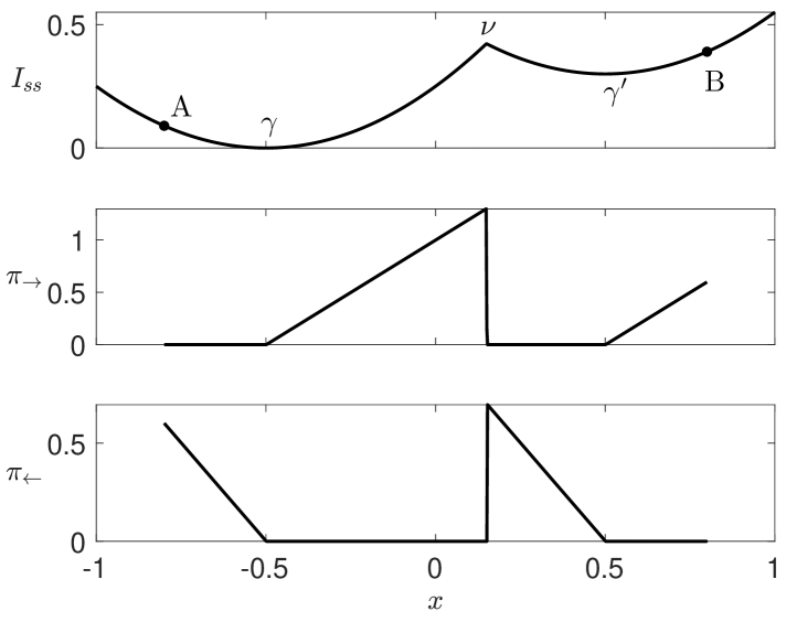
Figure 1: Illustration of quasipotential $I_{ss}$ in a bistable system (top), along with controls $\pi(x)$ to go from A to B (middle) and from B to A (bottom).

It follows from Eq.(5) that $I_{ss}$ is not smooth at the boundaries between basins. We call these boundaries ‘saddles’ although they may not be located at the saddles expected from a naive analysis. It was shown by Graham and Tél in a series of works that this non-smooth behavior is generic whenever the system is not in detailed balance, except in the special case when the $H=0$ manifold is integrable Graham and Tél (1984a, b, 1985, 1986) ( see review Baek and Kafri (2015)).

This phenomenon, which may initially appear exotic, has a natural interpretation from the control point of view. First we note that on uphill instantons we have $\vec{\pi}~=~\nabla I_{ss}$ , while on downhill instantons we have $\vec{\pi}=0$. This allows us to define a control $\vec{\pi}_{\eta}({\vec{n}})$ for the instantonic path $\eta$ from one state to another, where we must take the appropriate branch depending on whether we go uphill $({\vec{n}}\cdot\nabla I_{ss}>0)$ or downhill $({\vec{n}}\cdot\nabla I_{ss}<0)$. This is illustrated in Fig.1 for a schematic bistable system, for paths going from A to B and from B to A. The interpretation of $\vec{\pi}$ is clear: the system needs to be steered into the desired attractor. After passing through the saddle, the control can be turned off, as the system will relax freely to the fixed point. (To go further uphill beyond the fixed point, the control needs to be turned back on.) So $\nabla I_{ss}$ has no need to be smooth at saddles, and $I_{ss}$ can have kinks, as observed. Moreover it is natural to describe these paths as agentic (goal-directed).

This path-dependent $\vec{\pi}_{\eta}({\vec{n}})$ has a quantitative role since the transition rate $\kappa_{\gamma\gamma^{\prime}}^{\nu}$ from attractors $\gamma$ to $\gamma^{\prime}$ via the saddle $\nu$ can be written Falasco and Esposito (2025), in the macroscopic limit, as

$$\log\kappa_{\gamma\gamma^{\prime}}^{\nu} =-\Omega[I_{ss}^{(\gamma)}({\vec{n}}_{\nu})-I_{ss}^{(\gamma)}({\vec{n}}_{\gamma})]$$

$$=-\Omega\int_{\gamma}^{\nu}d{\vec{n}}\cdot\vec{\pi}$$ (6)

where the line integral is along the instanton up to the saddle. These rates in turn fix the constants $\{\alpha_{\gamma}\}$ appearing in Eq.(5) . The quantity $1/\kappa_{\gamma\gamma^{\prime}}^{\nu}$ is the mean-first-passage time, so that the timescale associated to a path $\eta$ is $\tau_{\eta}=e^{\Omega\int_{\eta}d{\vec{n}}\cdot\vec{\pi}_{\eta}}$. Control is paid for in time.

So far we have not imposed any conditions arising from thermodynamics, but they are readily incorporated with the stochastic thermodynamics (ST) formalism Seifert (2012); Freitas and Esposito (2022); Falasco and Esposito (2025). Under the standard assumptions of ST, and in the macroscopic limit, the transition rates between attractors $\{\kappa_{\gamma\gamma^{\prime}}^{\nu}\}$ can be bounded, both above and below, by components of entropy production along corresponding paths, viz., Freitas and Esposito (2022); Falasco and Esposito (2025)

$$-\sigma_{\nu\to\gamma}\leq\frac{1}{\Omega}\log\kappa_{\gamma\gamma^{\prime}}^{\nu}\leq\sigma_{\gamma\to\nu},$$

and these bounds are sharp both in the detailed balance case and to first order in nonconservative forces. Comparing with Eq.(Noise equals endogenous control) the control theoretic interpretation of $I_{ss}$ then establishes bounds between entropy production and integrated control. In particular the upper bound on $\kappa^{\nu}_{\gamma\gamma^{\prime}}$ indicates that for a large entropy drop, strong control is necessary. If local creation of negative entropy is necessary for life Schrödinger and Penrose (1992), then control plays an essential role.

Thermodynamic uncertainty relations state that for a current $O$ its variance and mean are related by $\langle O^{2}\rangle_{c}/\langle O\rangle^{2}\geq 2/\sigma$ where $\sigma$ is the entropy production in the process, in units of $k_{B}$ Barato and Seifert (2015); Horowitz and Gingrich (2020). This is usually read as saying that precision requires entropy dissipation. Since variances are related to noise, and hence to control, an alternative reading is that minimal entropy dissipation requires strong control .

This new perpective may help understand the largely unexplained thermodynamic efficiency of biological systems Kempes et al. (2017); Wolpert et al. (2024). Indeed the notion that in a biochemical system any particular species needs to be maintained at a precise concentration is usually a prejudice; the cell is apparently content to operate with significant copy-number fluctuations Elowitz et al. (2002). What is crucial is that the system continues to play the same functional role. By recasting noise as control, this shifts focus from seeking mechanisms that eliminate all fluctuations, or work in spite of them, to understanding the relationship between control and objective.

Unstable fixed points: Unstable systems can be stabilized by control. While much of physics is built on harmonic behavior around equilibria, when noise is added and interpreted as control, the restriction to stable equilibria is unnecessarily strict. A growing literature in the ecology Boettiger (2018) and systems biology Eldar and Elowitz (2010); Hilfinger et al. (2016) communities indeed finds that noise can act as a stabilizing force. Hitherto these have been given idiosyncratic explanations, if any. The noise-control mapping explored here instead makes it natural. To illustrate this, we consider in SI the control of unstable linear systems, paying attention to the form of the objective relevant for noisy systems. Unstable fixed points found already in the deterministic dynamics are not asymptotically stable under optimal control, and so eventually leave the vicinity of the fixed point. But there are also control-stabilized fixed points that do not exist deterministically, reflecting a balance between control and relaxation. When perturbed they perform a cycle, like Sisyphus pushing a boulder up a hill only for it to fall back to the bottom. The feedback for such cycles is not smooth: at some point it abruptly changes from $-\infty$ to $+\infty$, corresponding to pushing the deviation towards and then away from the fixed point.

In noisy systems, the dynamical role of control-stabilized fixed points is unclear. Yet, on topological grounds they are expected to be generic, and they capture the essential irreversible dynamics in a way that is impossible at a deterministic fixed point.

Discussion: We have argued that in any stochastic system, noise acts as endogenous control. To be informative about control problems faced by the cell, the objective that is optimised must be biologically meaningful. So consider, on general grounds, what is required for such an objective. First, we divide states into acceptable and unacceptable outcomes, and have a cost $\mathscr{G}({\vec{n}})>0$ for unacceptable outcomes. Let $\mathscr{G}({\vec{n}})=0$ when ${\vec{n}}$ is acceptable. Then, the natural control objective is to make the acceptable states maximally probable. For acceptable states, the objective will take the form $-\mathscr{F}(\mathbb{P}({\vec{n}}_{f}|{\vec{n}}_{0}))$ where $\mathscr{F}$ is increasing. Let us normalize the objective such that $\mathscr{F}(1)=0$. We demand that if states are separated into independent subsystems, then $\mathscr{F}$ is additive. This ensures that the pairwise optimal controls are equivalent to the joint optimal control. As is well known, these requirements imply that $\mathscr{F}(P)\propto\log P$ with a positive proportionality constant Shannon and Weaver (1964), which we take to be unity.

If for simplicity we consider $\mathscr{G}({\vec{n}})=\infty$ for unacceptable states, then this objective just reduces to maximizing $\mathbb{P}({\vec{n}}_{f})$ over acceptable ${\vec{n}}_{f}$, which is exactly the objective attained by weak noise. Moreover the $-\log\mathbb{P}$ form of objective is seen as crucial to understand how complex objectives are built from simple ones in composite systems.

Conclusion: Macroscopic stochastic systems perform optimal endogeneous control. The emergent long-time dynamics of a CRN with many attractors will involve active control. An example of this is given by a Lotka-Volterra ecosystem with random interactions Bunin (2017); De Giuli and Scalliet (2022). For large enough heterogeneity, the system is in a Parisi-Gardner phase with many metastable states, and chaotic dynamics Biroli et al. (2018); Pearce et al. (2019); Roy et al. (2020); Altieri et al. (2020); Garcia Lorenzana and Altieri (2022). Very recently a dynamical mean-field theory was obtained for the long-time dynamics Arnoulx de Pirey and Bunin (2024), and shown to be non-smooth, with instantonic near-extinctions playing an essential role in renewal of the ecosystem. This explicitly shows a balance between stability (weight of attractors) and control (hopping).

Finally, although the cybernetic approach Wiener (2019); Ashby (1956, 1991) pioneered the use of control theory in biology, it waned as it became divorced from the spectactular successes of reductionist molecular biology. The noise-control mapping elucidated here firmly grounds cybernetic ideas in a precise connection, valid at any scale, and which behaves well under coarse graining, because the long-time dynamics of a CRN is itself a jump process over attractors Vellela and Qian (2009); Smith (2020); Falasco and Esposito (2025). What remains is to understand the generic forms of the objective in realistic systems, and especially how these relate to dynamics (point (ii) in Dehghani (2024)). Indeed the noise-control mapping is expected to be most fruitful in the cases that are difficult to describe in any language, for example when the dynamics visits many metastable states, and is highly sensitive to external forcing.

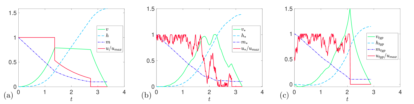
Figure 2: (a) Optimal control for Goddard problem, with 3 stages plainly visible; (b) Least-action trajectory in noisy Goddard system over an ensemble of 1000 trajectories; (c) Typical trajectory at $\beta=5$. These results take units with $g=h_{0}=m_{0}=1$ and parameters $u_{max}=1,c=\gamma=1/2,m_{1}=0.1$.

Supplementary Information.

Here we describe the Goddard rocket problem and its solution by a Langevin process (Appendix 1); the analytical approach to obtaining fluctuations around instantons, and their control-theoretic interpretation (Appendix 2); the use of the PMP to rederive the Hamiltonian equations for a CRN (Appendix 3); and the analysis and interpretation of unstable fixed points (Appendix 4).

Appendix 1. Goddard rocket problem:

Consider a rocket at with vertical velocity $v(t)$ at height $h(t)$, with total mass $m(t)$ (including both fuel and chassis). They evolve according to Newton’s laws

$$\partial_{t}v =\frac{1}{m}\left[u-D(v,h)\right]-g$$ (7a)

$$\partial_{t}h =v$$ (7b)

$$\partial_{t}m =-\gamma u,$$ (7c)

where $u(t)$ is the thrust control, $D(v,h)$ is the drag, and $\gamma$ is an efficiency coefficent. We start at sea level $v(0)=h(0)=0$ and with mass $m(0)=m_{0}$. The Goddard problem is to maximize the height obtained, $h(t_{f})$ where the final time is when the fuel runs out $m(t_{f})=m_{1}$ and the velocity vanishes $v(t_{f})=0$, where it is understood that $m_{1}$ is the mass of the chassis only. The thrust is subject to $0\leq u\leq u_{max}$.

The solution to this optimal control problem is highly nontrivial Glad and Ljung (2018). Indeed, although naively it might seem optimal to burn fuel as quickly as possible, to avoid carrying it unnecessarily to higher altitudes, when drag is factored in this is not necessarily true: it may be worth it to carry some fuel higher, where air is thinner and drag is reduced (or simply to burn it at a slower speed). It turns out that the optimal trajectory has generally 3 stages: a first ‘full throttle’ stage in which $u=u_{max}$; a second stage in which the control is nontrivial; and a final stage in which fuel is spent and the rocket decelerates to its maximum height.

Here we want to show that this solution can be approximated by a Langevin process, which we call the noisy Goddard system. We simply take Eq.(7) and model $u$ as noise. We consider it to be continuous with uncorrelated increments $du\in[-1,1]\times\sqrt{dt}$ where in the numerics we have $dt=0.01$. We impose $0\leq u(t)\leq u_{max}$. To compare with the optimal control, we turn the control off once $m(t)=m_{1}$.

In the numerics we take units in which $g=m_{0}=1$, and we fix a drag law $D(v,h)=cv^{2}e^{-h/h_{0}}$. We fix a length by $h_{0}=1$. In this problem there is no natural way to scale the noise that would still admit solutions in the weak-noise regime: for example if $u_{max}$ is too small then the rocket cannot gain altitude. In the numerics we sample paths with $e^{-\beta h(t_{f})}$ where $\beta$ can be adjusted. (The optimal control is of course independent of $\beta$.)

Fig.2 shows the results. At left is shown the optimal control with its 3 stages; at center is the best trajectory in a run of 1000 noisy trajectories (this result is typical over ensembles of this size); and at right is a median trajectory closest to the ensemble at $\beta=5$. These 3 trajectories give $h(t_{f})=1.58,1.39,$ and $1.15$, respectively. We see that the optimal control is well approximated by a noisy trajectory and comes within 15% of the maximum height. These results are typical, and illustrate that this control problem can be solved – within approximation, at a finite number of trajectories, and finite $\beta$ – by a noisy system.

Appendix 2. Gaussian fluctuations around instantons:

Consider, either for Langevin dynamics or Markov jump processes,

$$S({\vec{n}},\vec{\pi})=\int dt\;\left[\vec{\pi}\cdot\partial_{t}{\vec{n}}-H({\vec{n}},\vec{\pi})\right]$$

where $H({\vec{n}},0)=0$ and we suppress boundary conditions ${\vec{n}}(0)={\vec{n}}_{0},{\vec{n}}(t_{f})={\vec{n}}_{f}$.

For Langevin dynamics $H$ takes the form

$$H({\vec{n}},\vec{\pi})=-\vec{\pi}\cdot\vec{V}({\vec{n}})+\mbox{$\frac{1}{2}$}\vec{\pi}\cdot B\cdot B^{T}\cdot\vec{\pi}\qquad\text{Langevin}$$

while for CRNs each reaction $\alpha$ of the form $\sum p_{\alpha j}X_{j}\to\sum q_{\alpha j}X_{j}$ ($X_{j}$ denote the species) contributes

$$H_{\alpha}({\vec{n}},\vec{\pi})=(e^{\vec{\pi}\cdot(\vec{q}_{\alpha}-\vec{p}_{\alpha})}-1)\tilde{k}_{\alpha}\prod_{i}n_{i}^{p_{\alpha i}}\qquad\text{CRN}$$

where $\tilde{k}_{\alpha}$ is a rescaled reaction rate (see De Giuli and Scalliet (2022)). These specific forms will not be needed in this section.

We set ${\vec{n}}={\vec{n}}_{*}+{\vec{n}}^{\prime}$ and $\vec{\pi}=\vec{\pi}_{*}+\vec{\pi}^{\prime}$ and look at the regime of small ${\vec{n}}^{\prime},\vec{\pi}^{\prime}$, which is relevant in the macroscopic limit. To quadratic order in ${\vec{n}}^{\prime},\vec{\pi}^{\prime}$ we obtain

$$S({\vec{n}},\vec{\pi}) =S_{*}+\int dt\;\left[\vec{\pi}_{*}\cdot\partial_{t}{\vec{n}}^{\prime}+\vec{\pi}^{\prime}\cdot\partial_{t}{\vec{n}}_{*}+\vec{\pi}^{\prime}\cdot\partial_{t}{\vec{n}}^{\prime}\right.$$

$$\left.-{\vec{n}}^{\prime}\cdot\nabla_{n}H-\vec{\pi}^{\prime}\cdot\nabla_{\pi}H-{\vec{n}}^{\prime}\vec{\pi}^{\prime}:\nabla_{n}\nabla_{\pi}H\right.$$

$$\left.-\mbox{$\frac{1}{2}$}{\vec{n}}^{\prime}{\vec{n}}^{\prime}:\nabla_{n}\nabla_{n}H-\mbox{$\frac{1}{2}$}\vec{\pi}^{\prime}\vec{\pi}^{\prime}:\nabla_{\pi}\nabla_{\pi}H\right]+\ldots$$

where $S_{*}=S({\vec{n}}_{*},\vec{\pi}_{*})$ and the derivatives of $H$ are evaluated on $({\vec{n}}_{*},\vec{\pi}_{*})$. Choosing the latter to satisfy the instanton equations Eq.(4) this is reduced to

$$S \to S_{*}+\int dt\;\left[\vec{\pi}^{\prime}\cdot\partial_{t}{\vec{n}}^{\prime}-\vec{\pi}^{\prime}{\vec{n}}^{\prime}:A\right.$$

$$\left.\qquad-\mbox{$\frac{1}{2}$}{\vec{n}}^{\prime}{\vec{n}}^{\prime}:K-\mbox{$\frac{1}{2}$}\vec{\pi}^{\prime}\vec{\pi}^{\prime}:C\right]$$

$$\to S_{*}+\int dt\;\vec{\pi}^{\prime}\cdot\left[\partial_{t}{\vec{n}}^{\prime}-{\vec{n}}^{\prime}\cdot A-\vec{\xi\;}\cdot C\right]$$

$$\qquad+\mbox{$\frac{1}{2}$}\int dt\;\left[-{\vec{n}}^{\prime}{\vec{n}}^{\prime}:K+\vec{\xi\;}\vec{\xi\;}:C\right]$$

where in the last step we performed a Hubbard-Stratonovich transformation to introduce $\vec{\xi\;}$. Here

$$A =\nabla_{\pi}\nabla_{n}H$$

$$K =\nabla_{n}\nabla_{n}H$$

$$C =\nabla_{\pi}\nabla_{\pi}H.$$

If we integrate out $\vec{\pi}^{\prime}$ then we obtain a new Langevin equation that is linear in ${\vec{n}}^{\prime}$ but generally non-autonomous, viz.,

$$\partial_{t}{\vec{n}}^{\prime}-A\cdot{\vec{n}}^{\prime}=C\cdot\vec{\xi\;}$$ (8)

Moreover the objective function now has two terms

$$S_{2}=\int dt\;\left[-\mbox{$\frac{1}{2}$}{\vec{n}}^{\prime}{\vec{n}}^{\prime}:K+\mbox{$\frac{1}{2}$}\vec{\xi\;}\vec{\xi\;}:C\right]$$ (9)

Now since $H({\vec{n}},0)=0$, we have $K=\nabla_{n}\nabla_{n}H=0$ on deterministic trajectories $\vec{\pi}_{*}=0$: it is only present under active control.

The remaining problem is to integrate out $({\vec{n}}^{\prime},\vec{\xi\;})$ (or equivalently $({\vec{n}}^{\prime},\vec{\pi}^{\prime})$). If the boundary conditions on ${\vec{n}}^{\prime}$ are null, because they have already been accounted for in ${\vec{n}}_{*}$, then the result will only contribute the term in $S_{2}$ quadratic in ${\vec{n}}^{\prime}$, and a (functional) determinant, which can be evaluated Gel’fand and Yaglom (1960); Dunne (2008).

For simplicity consider the case when $({\vec{n}}_{*},\vec{\pi}_{*})$ is a fixed point, so that $A,K,C$ are all constant matrices. Then the result is Schorlepp et al. (2021)

$$\mathbb{P}({\vec{n}}_{f}|{\vec{n}}_{0})\propto e^{-S_{*}}e^{\frac{1}{2}\int Q:K}\left[\det Q(t_{f})\right]^{-1/2}$$ (10)

where $Q(t)$ satisfies

$$\partial_{t}Q=Q\cdot A^{T}+A\cdot Q+C+Q\cdot K\cdot Q$$ (11)

with $Q(0)=0$. Eq.(10) also holds in more general conditions when the dynamics is nonlinear and can include multiplicative noise. In the latter case some renormalization of the determinant is necessary Schorlepp and Grafke (2025).

To understand the physical meaning of $Q$, we consider the Hamiltonian form of Eqs.(8,9), viz.,

$$\partial_{t}{\vec{n}}^{\prime} =A\cdot{\vec{n}}^{\prime}+C\cdot C^{T}\cdot\vec{\pi}$$

$$\partial_{t}\vec{\pi} =-A^{T}\cdot\vec{\pi}.$$

Construct a basis set of solutions satisfying ${\vec{n}}^{\prime(k)}(0)=0,\pi^{(k)}_{j}(0)=\delta_{jk}$. These correspond to all the directions that can be reached from ${\vec{n}}^{\prime}(0)=0$. These can be placed as columns into matrices $\delta N,\delta\Pi$. Then the matrix

$$Q^{\prime}=\delta N\cdot(\delta\Pi)^{-1}$$ (12)

satisfies the same equation Eq.(11). Since $\delta N(0)=0$, we get also that $Q^{\prime}(0)=0$, so $Q^{\prime}=Q$.

From Eq.(12) we can write $\delta\Pi=(Q^{\prime})^{-1}\cdot\delta N$, meaning $\vec{\pi}^{(k)}=(Q^{\prime})^{-1}\cdot{\vec{n}}^{(k)}$. In other words, these solutions take a feedback form where $(Q^{\prime})^{-1}$ is the feedback matrix giving the controls in terms of the state fluctuation.

This argument extends straightforwardly to any situation for which Eq.(10) holds, including cases where the instanton ${\vec{n}}_{*}$ is time-dependent.

Appendix 3: Pontryagin Minimum Principle:

The Pontryagin maximum principle (PMP) states that, for Eqs.(1,2) and general $L$, the optimal control must maximize the Pontryagin Hamiltonian

$$H_{P}({\vec{n}},\vec{\xi\;},\vec{p},t)=\vec{p}\cdot[B({\vec{n}})\cdot\vec{\xi\;}-\vec{V}({\vec{n}})]-L[{\vec{n}},\vec{\xi\;}]$$

pointwise in $\vec{\xi\;}$, where $\vec{p}$ solves the costate equations $\partial_{t}\vec{p}=-\nabla_{n}H_{P}$. In the Langevin case $L=\mbox{$\frac{1}{2}$}\vec{\xi\;}^{2}$ the maximization of $H_{P}$ leads to $\vec{\xi\;}=-\vec{p}\cdot B({\vec{n}})$ and then $H_{P}\to\mbox{$\frac{1}{2}$}\vec{p}\cdot B\cdot B^{T}\cdot\vec{p}+\vec{p}\cdot\vec{V}=H$ when we identify $\vec{p}=-\vec{\pi}$. As expected we recover Eq.(4) but without path integral manipulations.

For Markov jump processes we consider the PMP with objective $\int L$ with $L({\vec{n}},\vec{\pi})=\vec{\pi}\cdot\nabla_{\pi}H-H$ and field equation $\partial_{t}{\vec{n}}=\nabla_{\pi}H$. We have

$$H_{P}({\vec{n}},\vec{\pi},\vec{p},t) =\vec{p}\cdot\nabla_{\pi}H-L({\vec{n}},\vec{\pi})$$

$$=(\vec{p}-\vec{\pi})\cdot\nabla_{\pi}H+H({\vec{n}},\vec{\pi})$$

and the costate equation is

$$\partial_{t}\vec{p} =-\nabla_{n}H_{P}$$

$$=(\vec{\pi}-\vec{p})\cdot\nabla_{\pi}\nabla_{n}H-\nabla_{n}H.$$

Extremizing $H_{P}$ over $\vec{\pi}$ we get

$$0=\nabla_{\pi}H_{P}=(\vec{p}-\vec{\pi})\cdot\nabla_{\pi}\nabla_{\pi}H,$$

solved by $\vec{p}=\vec{\pi}$. Then the costate equation reduces to $\partial_{t}\vec{\pi}=-\nabla_{n}H$, which is the correct equation. Moreover the objective becomes $\int L\to\int[\vec{\pi}\cdot(\partial_{t}{\vec{n}})-H]=S$ as required.

Appendix 4: Unstable modes:

Consider the linear system Eq.(8) with objective Eq.(9), where the matrix $A$ may have unstable modes. We let the boundary conditions be ${\vec{n}}^{\prime}(0)={\vec{n}}_{0},{\vec{n}}^{\prime}(t_{f})={\vec{n}}_{f}$. We are assuming that $A,C,$ and $K$ are time-independent, which will hold if we apply this formalism to the linear dynamics around fixed points. Importantly, these may include non-classical fixed points where $\vec{\pi}_{*}\neq 0$, as discussed later. In the language of control theory this is a linear-quadratic regulator (LQR). (One can also drop the final boundary condition and replace it with a cost on the final state).

Consider the feedback form

$$\vec{\xi\;}=-R\cdot{\vec{n}}^{\prime}$$ (13)

so that the so-called closed-loop dynamics for ${\vec{n}}^{\prime}$ becomes

$$\partial_{t}{\vec{n}}^{\prime}=\underbrace{(A-C\cdot R)}_{M}\cdot{\vec{n}}^{\prime}.$$

This closed-loop dynamics will be asymptotically stable if $M$ is Hurwitz, i.e. all its eigenvalues have negative real part. It is known from control theory that if the system is controllable (which is expected to be the usual case in noisy systems), then we can define $R=C^{T}\cdot W^{-1}$ where

$$W(t)=\int_{0}^{t}ds\;e^{-sA}\cdot C\cdot C^{T}\cdot e^{-sA^{T}},$$

and $M$ will be Hurwitz . Note that

$$A\cdot W(t) =-\int_{0}^{t}ds\;\partial_{s}[e^{-sA}]\cdot C\cdot C^{T}\cdot e^{-sA^{T}}$$

$$=-e^{-tA}\cdot C\cdot C^{T}\cdot e^{-tA^{T}}+C\cdot C^{T}$$

$$\qquad+\int_{0}^{t}ds\;e^{-sA}\cdot C\cdot C^{T}\cdot\partial_{s}[e^{-sA^{T}}]$$

$$=-\partial_{t}W(t)+C\cdot C^{T}-W(t)\cdot A^{T},$$

i.e.

$$\partial_{t}W(t)=A\cdot W(t)+W(t)\cdot A^{T}+C\cdot C^{T}$$ (14)

To illustrate, we focus on the case when $A$, $C$, and $K$ are the same size, and simultaneously diagonalizable, so that modes are independent. Then we write

$$A =\sum_{\lambda}\lambda|\lambda\rangle\langle\lambda|$$

$$C =\sum_{\lambda}c_{\lambda}|\lambda\rangle\langle\lambda|$$

$$K =\sum_{\lambda}k_{\lambda}|\lambda\rangle\langle\lambda|$$

$$W =\sum_{\lambda}w_{\lambda}(t)|\lambda\rangle\langle\lambda|$$

where we adopt a bra-ket notation. We assume that $A$ has no zero modes; the limit $\lambda\to 0$ can be taken later if necessary. For each mode we have

$$w_{\lambda}(t)=c_{\lambda}^{2}\int_{0}^{t}dte^{-2t\lambda}=\frac{c_{\lambda}^{2}}{2\lambda}\left[1-e^{-2t\lambda}\right]$$

and we find that the eigenvalues of $M$ are

$$m_{\lambda}(t) =\lambda-c_{\lambda}^{2}w_{\lambda}(t)^{-1}$$

$$=\lambda-\frac{2\lambda}{1-e^{-2t\lambda}}$$

$$\xrightarrow[t\to\infty]{}\begin{cases}-\lambda&Re[\lambda]>0\\ +\lambda&Re[\lambda]<0\end{cases}$$

so that the system is stabilized. However, this form of regulator is not necessarily the optimal control, because it ignores the objective, and will not generically fit the boundary conditions.

It turns out that the optimal control still has the form Eq.(13), but the matrix $R$ satisfies

$$\partial_{t}R=-A^{T}\cdot R-R\cdot A+R\cdot C\cdot R+K$$

If we define

$$Q=-R^{-1}$$

and use the identity $\partial_{t}R^{-1}=-R^{-1}\cdot\partial_{t}R\cdot R^{-1}$ then we obtain

$$\partial_{t}Q =R^{-1}\cdot\partial_{t}R\cdot R^{-1}$$

$$=R^{-1}\cdot\left[-A^{T}\cdot R-R\cdot A+R\cdot C\cdot R+K\right]\cdot R^{-1}$$

$$=Q\cdot A^{T}+A\cdot Q+C+Q\cdot K\cdot Q$$

which is exactly Eq.(11) above. We note the similarity with Eq.(14), but also the differences, namely the absence there of a quadratic term, whose role will be explained below.

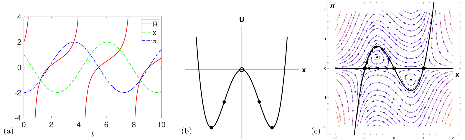
Figure 3: (a) Illustration of cycle around control-stabilized unstable fixed point. (b) Double well potential, with deterministic and control-stabilized fixed points indicated. (c) Phase portrait of double well oscillator. The $H=0$ manifold is shown in bold. This includes both deterministic trajectories at $\pi=0$ and the uphill instantons. The instantons from $x=-1$ to $x=0$ and back are indicated with arrows.The cycles around the control-stabilized fixed points are clear.

Writing

$$Q =\sum_{\lambda}q_{\lambda}(t)|\lambda\rangle\langle\lambda|$$

$${\vec{n}}^{\prime} =\sum_{\lambda}x_{\lambda}(t)|\lambda\rangle,$$

for each mode we have

$$\partial_{t}q_{\lambda}=2\lambda q_{\lambda}+c_{\lambda}+k_{\lambda}q_{\lambda}^{2}$$

with solution

$$q_{\lambda}(t) =\begin{cases}-\frac{c_{\lambda}}{2\lambda}+c_{1,\lambda}e^{2\lambda t}&k_{\lambda}=0\\ \frac{-\lambda}{k_{\lambda}}+\frac{\sqrt{c_{\lambda}k_{\lambda}-\lambda^{2}}}{k_{\lambda}}\tan\left((t-t_{0,\lambda})\sqrt{c_{\lambda}k_{\lambda}-\lambda^{2}}\right)&k_{\lambda}\neq 0\end{cases}$$

where $c_{1,\lambda}$ and $t_{0,\lambda}$ are fixed by boundary conditions.

The cases $k_{\lambda}=0$ and $k_{\lambda}\neq 0$ are fundamentally different.

Case (i): $k_{\lambda}=0$ : For $k_{\lambda}=0$ we find

$$m_{\lambda}(t) =\lambda+c_{\lambda}q_{\lambda}(t)^{-1}$$

$$=\lambda+c_{\lambda}\frac{1}{-\frac{c_{\lambda}}{2\lambda}+c_{1,\lambda}e^{2\lambda t}}$$

Write $c_{1,\lambda}=-\frac{c_{\lambda}}{2\lambda}e^{-2\lambda t_{f}}c^{\prime}_{\lambda}$ so that

$$m_{\lambda}(t) =\lambda\left[1-\frac{2}{1+c^{\prime}_{\lambda}e^{2\lambda(t-t_{f})}}\right]$$

Now we have

$$\partial_{t}[\log x_{\lambda}(t)]=m_{\lambda}(t)$$

which is integrated to obtain

$$x_{\lambda}(t)=x_{\lambda}(0)e^{\lambda t}\lambda\left(c^{\prime}_{\lambda}+e^{-2\lambda(t-t_{f})}\right)$$

We are primarily interested in the stability problem ${\vec{n}}^{\prime}(t_{f})=0$, i.e. $x_{\lambda}(t_{f})=0$. We see that if $c^{\prime}_{\lambda}=-1$ then we will have $x_{\lambda}(t_{f})=0$. This is so despite the fact that

$$m_{\lambda}(t) \xrightarrow[t\to\infty]{}\begin{cases}+\lambda&\text{Re}[\lambda]>0\\ -\lambda&\text{Re}[\lambda]<0\end{cases}$$

which is asymptotically unstable! This means that for a given horizon $t_{f}$ we can always control the system back to the fixed point, but if the control protocol remains on, then eventually the system will leave the fixed point. To control unstable fixed points with $k_{\lambda}=0$ we then need to be eternally vigilant. Contrast this with the second case

Case (ii): $k_{\lambda}\neq 0$ : Now we find

$$m_{\lambda}(t)=\lambda+\begin{cases}\frac{c_{\lambda}k_{\lambda}}{-\lambda+\sqrt{c_{\lambda}k_{\lambda}-\lambda^{2}}\tan\left((t-t_{0,\lambda})\sqrt{c_{\lambda}k_{\lambda}-\lambda^{2}}\right)}&\text{Re}[c_{\lambda}k_{\lambda}-\lambda^{2}]>0\\ \frac{c_{\lambda}k_{\lambda}}{-\lambda-\sqrt{\lambda^{2}-c_{\lambda}k_{\lambda}}\tanh\left((t-t_{0,\lambda})\sqrt{\lambda^{2}-c_{\lambda}k_{\lambda}}\right)}&\text{R}e[c_{\lambda}k_{\lambda}-\lambda^{2}]<0\end{cases}$$

whose behavior depends on the sign of Re$[c_{\lambda}k_{\lambda}-\lambda^{2}]$.

If $c_{\lambda}k_{\lambda}-\lambda^{2}<0$, then $m_{\lambda}(t)\to\sqrt{\lambda^{2}-c_{\lambda}k_{\lambda}}$ as $t\to\infty$, so it is asymptotically unstable, and all the caveats of the first case apply.

Instead if $c_{\lambda}k_{\lambda}-\lambda^{2}>0$, then the system oscillates in a highly nonlinear way. Moreover, it is insensitive to the boundary conditions so the control protocol can remain on. This regime is quite remarkable in that $m_{\lambda}(t)$ has infinitely many singularities. An example is shown in Fig.3a for $\lambda=1/2,c_{\lambda}=1,k_{\lambda}=2$. The regulator is out of phase with the state, so the feedback has singularities.

To see these ideas in action, we consider a double well potential $U(x)=-\mbox{$\frac{1}{2}$}ax^{2}+\frac{1}{4}bx^{4}$, pictured in Fig.3b. The Hamiltonian is

$$H(x,\pi)=\pi(ax-bx^{3})+\mbox{$\frac{1}{2}$}\pi^{2}$$

and the instanton equations are

$$\partial_{t}x =ax-bx^{3}+\pi$$

$$\partial_{t}\pi =-\pi(a-3bx^{2})$$

The phase portrait is shown in Fig.3c.

Looking for fixed points we find five: the two stable minima, $x=\pm\sqrt{a/b}$, with $\pi=0$; the unstable saddle $x=0$ with $\pi=0$; and two non-classical fixed points $x=\pm\sqrt{a/3b}$ with $\pi=-2ax/3$. Now as mentioned above, due to the general property $H({\vec{n}},0)=0$, we get that $K=0$ on all deterministic fixed points, where $\pi=0$. It follows that the behavior near the fixed points follows that of case (i) above. Instead at the non-classical fixed points we find $K=4a^{2}/3>0$ and $A=0$ so case (ii) is relevant. The cycles look qualitatively like those shown in Fig.3a. The phase shift and relative amplitude of state and control depend on the parameters.

Such control-stabilized fixed points (more generally manifolds) are expected to be generic. Indeed, consider a deterministic fixed point $\gamma$ and one of its saddles $\nu$. From $\nu$ down to $\gamma$ there is a manifold along $\vec{\pi}=0$ giving the relaxation trajectory. The ‘uphill’ trajectory instead is at $\vec{\pi}\neq 0$, so these two manifolds enclose a volume, with a circulation flux, because their trajectories are oriented in the opposite way. Both of these manifolds have $H=0$. The enclosed volume can be followed in contours of $H$ until it collapses on a manifold of lower dimension, for example a fixed point in 2D. This is the control-stabilized manifold.